from the lab to the real world : sources of error in uf6
TRANSCRIPT
University of New MexicoUNM Digital Repository
Nuclear Engineering ETDs Engineering ETDs
7-5-2012
From the lab to the real world : sources of error inUF6 gas enrichment monitoringMarcie Lombardi
Follow this and additional works at: https://digitalrepository.unm.edu/ne_etds
This Dissertation is brought to you for free and open access by the Engineering ETDs at UNM Digital Repository. It has been accepted for inclusion inNuclear Engineering ETDs by an authorized administrator of UNM Digital Repository. For more information, please contact [email protected].
Recommended CitationLombardi, Marcie. "From the lab to the real world : sources of error in UF6 gas enrichment monitoring." (2012).https://digitalrepository.unm.edu/ne_etds/17

i
Marcie L. Lombardi _________________________________________________________________ Candidate
Chemical and Nuclear Engineering __________________________________________________________________ Department
This dissertation is approved, and it is acceptable in quality and form for publication:
Approved by the Dissertation Committee:
Adam Hecht
Gary Cooper
Plamen Atanassov
Duncan MacArthur
ii
FROM THE LAB TO THE REAL WORLD: SOURCES OF ERROR IN UF6 GAS ENRICHMENT MONITORING
by
MARCIE L. LOMBARDI
B.S., Physics, Rutgers University, 2002 M.S., Health Physics, Georgetown University, 2006
DISSERTATION
Submitted in Partial Fulfillment of the Requirements for the Degree of
Doctor of Philosophy
Engineering
The University of New Mexico Albuquerque, New Mexico
March 2012

iii
DEDICATION
This dissertation is dedicated to my aunt Shari Troy. I wish you could have seen it completed.

iv
ACKNOWLEDGEMENTS
I’d like to thank my dissertation committee at the University of New Mexico,
Adam Hecht, Gary Cooper and Plamen Atanassov. I must thank Duncan MacArthur for
serving on my committee, but also for the many hours of guidance, editing, and moral
support.
I would like to thank Kiril Ianakiev for his great ideas and allowing me to work
on his projects, as well as the whole enrichment monitoring team at Los Alamos. I
learned so much while working on this project, and got to go on a trip to England!
Brian Rees – thanks for keeping me motivated. I knew I could always count on
you for an “are you done yet??” On that note, I would like to thank all of my coworkers
and friends at LANL for their support and encouragement along the way.
Finally, and most importantly, I’d like to thank my friends and family for their
support and understanding during this stressful time in my life. I thank my parents for
always encouraging me. Last but not least, I’d like to give a special thanks to Nicole, my
biggest fan.
v
From the Lab to the Real World: Sources of Error in UF6 Gas Enrichment Monitoring
Marcie L. Lombardi
B.S., Physics, Rutgers University, 2002
M.S., Health Physics, Georgetown University, 2006 Ph.D., Engineering, University of New Mexico, 2012
ABSTRACT
Safeguarding uranium enrichment facilities is a serious concern for the
International Atomic Energy Agency (IAEA). Safeguards methods have changed over the
years, most recently switching to an improved safeguards model that calls for new
technologies to help keep up with the increasing size and complexity of today’s gas
centrifuge enrichment plants (GCEPs). One of the primary goals of the IAEA is to detect
the production of uranium at levels greater than those an enrichment facility may have
declared. In order to accomplish this goal, new enrichment monitors need to be as
accurate as possible.
This dissertation will look at the Advanced Enrichment Monitor (AEM), a new
enrichment monitor designed at Los Alamos National Laboratory. Specifically explored
are various factors that could potentially contribute to errors in a final enrichment
determination delivered by the AEM. There are many factors that can cause errors in the
determination of uranium hexafluoride (UF6) gas enrichment, especially during the
period when the enrichment is being measured in an operating GCEP. To measure
enrichment using the AEM, a passive 186-keV (kiloelectronvolt) measurement is used to
determine the 235U content in the gas, and a transmission measurement or a gas pressure
vi
reading is used to determine the total uranium content. A transmission spectrum is
generated using an x-ray tube and a “notch” filter.
In this dissertation, changes that could occur in the detection efficiency and the
transmission errors that could result from variations in pipe-wall thickness will be
explored. Additional factors that could contribute to errors in enrichment measurement
will also be examined, including changes in the gas pressure, ambient and UF6
temperature, instrumental errors, and the effects of uranium deposits on the inside of the
pipe walls will be considered. The sensitivity of the enrichment calculation to these
various parameters will then be evaluated. Previously, UF6 gas enrichment monitors have
required empty pipe measurements to accurately determine the pipe attenuation (the pipe
attenuation is typically much larger than the attenuation in the gas). This dissertation
reports on a method for determining the thickness of a pipe in a GCEP when obtaining an
empty pipe measurement may not be feasible.
This dissertation studies each of the components that may add to the final error in
the enrichment measurement, and the factors that were taken into account to mitigate
these issues are also detailed and tested. The use of an x-ray generator as a transmission
source and the attending stability issues are addressed. Both analytical calculations and
experimental measurements have been used. For completeness, some real-world analysis
results from the URENCO Capenhurst enrichment plant have been included, where the
final enrichment error has remained well below 1% for approximately two months.

vii
Table of Contents
ABSTRACT ........................................................................................................................ v
Table of Contents .............................................................................................................. vii
List of Figures ..................................................................................................................... x
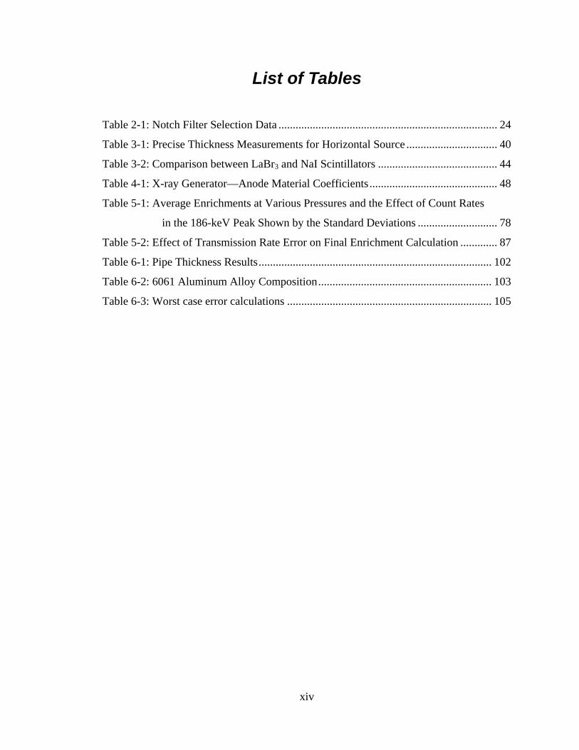
List of Tables ................................................................................................................... xiv
List of Abbreviations ........................................................................................................ xv
1 Introduction ................................................................................................................ 1
1.1 Safeguards for Uranium Enrichment Facilities ..............................................1
1.1.1 GCEP Basics ....................................................................................3
1.1.2 GCEP Proliferation Concerns ..........................................................5
1.2 Traditional Enrichment Measurement Methods .............................................6
1.3 X-ray Generator as a Transmission Source ....................................................7
1.4 Description of Dissertation Research .............................................................8
1.4.1 Calibration Method for Unknown Pipe Thickness ........................10
1.4.2 Sensitivity to Changes in Temperature and Pressure during
Measurement .................................................................................11
1.4.3 Field Trial—Some “Real-World” Data .........................................12
1.5 Similar Concepts in Industry and Medicine .................................................14
1.5.1 Dual X-ray Absorptiometry ...........................................................14
1.5.2 Two Gamma-ray Wall Thickness Gauge ......................................15
1.5.3 Two-Media Method for Attenuation Coefficient Measurement ....16
1.6 Outline of Dissertation ..................................................................................17
2 X-ray Measurement Concepts .................................................................................. 21
2.1 X-ray Tube Operation with a Bremsstrahlung Notch Filter .........................21
2.2 Attenuation of X-rays in Aluminum and Uranium Hexafluoride .................24
2.3 Calibration Method for Determining Pipe Thickness ...................................25
2.4 Addressing Potential X-ray Tube Instability ................................................29
3 Experimental Implementation .................................................................................. 31
3.1 Introduction ...................................................................................................31
viii
3.2 X-ray Tube and Collimator ...........................................................................33
3.3 Notch Filters .................................................................................................35
3.4 Flux Monitor .................................................................................................37
3.5 UF6 Source ....................................................................................................38
3.6 Detectors/MCAs ...........................................................................................43
4 Analytical Modeling and Calculations ..................................................................... 45
4.1 X-ray Tube ....................................................................................................45
4.1.1 Generated and Transmitted Spectra ...............................................46
4.1.2 Issues with Analytical Model ........................................................48
4.2 UF6 Properties ...............................................................................................51
4.3 Effect of Wall Deposits on Measurements ...................................................52
4.4 Flux Monitor Diode ......................................................................................55
4.4.1 Diode Responsivity ........................................................................56
4.4.2 Measurement Dose Rate ................................................................58
5 Experimental Measurements .................................................................................... 60
5.1 Flux Monitor Diode Measurements ..............................................................60
5.1.1 Long-term Irradiation Measurement..............................................60
5.1.2 I-V Characterization, Diode Recovery ..........................................62
5.2 Dual-Energy X-Ray Measurements ..............................................................65
5.2.1 UF6 Calibration Source ..................................................................65
5.2.2 Transmission Measurements .........................................................67
5.2.3 Gamma-ray Spectra .......................................................................68
5.3 Sensitivity to Changes in Pressure and Temperature during Measurement .74
5.3.1 Pressure ..........................................................................................74
5.3.2 Temperature Correction: Using the Flux Monitor .........................83
5.3.3 Temperature Correction: Simple Method ......................................85
5.4 Field Trial—URENCO Capenhurst ..............................................................89
5.4.1 Variations in UF6 Gas Pressure during Measurement ...................91
5.4.2 Background Determination (Including Pipe Deposits)..................92
5.4.3 Temperature Effects.......................................................................93
6 Pipe-wall Thickness Results and Analysis ............................................................... 95
ix
6.1 Experimental Results ....................................................................................95
6.2 Calibration Curve ..........................................................................................98
6.3 “Unknown” Pipe Thickness Measurements ...............................................100
6.4 Comparison between Analytical/Experimental Results .............................102
7 Error Analysis ......................................................................................................... 106
7.1 Errors in Determining Pipe-wall Thickness ................................................106
7.1.1 “Unknown” Pipe Thicknesses Measurement ...............................106
7.1.2 Measured Ratios ..........................................................................107
7.1.3 “Unknown” Pipe Thicknesses Calculation ..................................110
7.2 Enrichment Error from Wall Thickness Measurement Error .....................111
7.3 Enrichment Errors over Time (Passive System) .........................................116
8 Conclusions ............................................................................................................ 119
9 Future Work ............................................................................................................ 121
Appendices .......................................................................................................................122
Appendix A: Mass Attenuation Coefficients .............................................................123
Appendix B: Equipment Specifications .....................................................................126
Appendix C: MCNPX Input File—Diode Flux .........................................................131
References ........................................................................................................................133

x
List of Figures
Figure 1-1: Simplified diagram of an enrichment cascade ................................................. 3
Figure 1-2: Hypothetical cascade arrangement showing the variation in the number of
centrifuges in each stage ................................................................................ 4
Figure 2-1: Notch filter concept ........................................................................................ 21
Figure 2-2: Attenuation as a function of energy in UF6 gas and the aluminum pipe. ...... 25
Figure 2-3: Calculated energy-dependent bremsstrahlung yield of the x-ray tube for
varying cutoff energies. ............................................................................... 26
Figure 2-4: Transmitted spectra as calculated from Eqn. (3), with molybdenum and
palladium notch filter thicknesses of 0.05 cm. ............................................ 27
Figure 2-5: Ratios of the transmitted spectra as a function of UF6 gas pressure .............. 28
Figure 2-6: Part of the experimental setup for the diode test ............................................ 30
Figure 3-1: Active AEM setup with LaBr3 detector ......................................................... 32
Figure 3-2: Passive AEM setup with NaI detectors .......................................................... 33
Figure 3-3: The x-ray tube mounted in the active measurement head .............................. 34
Figure 3-4: Underside of the active head showing the flux monitor diode mounted in
place ............................................................................................................. 35
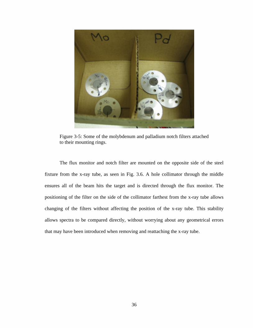
Figure 3-5: Some of the molybdenum and palladium notch filters attached to their
mounting rings. ............................................................................................ 36
Figure 3-6: A filter in place in the base of the active head. .............................................. 37
Figure 3-7: Flux monitor diode in its PEEK holder .......................................................... 38
Figure 3-8: Large horizontal UF6 source with three pipe thicknesses, variable gas
pressure, and variable enrichment ................................................................ 40
Figure 3-9: Horizontal UF6 source showing the three pipe thickness “steps.” ................. 41
Figure 3-10: Vertical UF6 source in the environmental chamber ..................................... 42
Figure 3-11: Typical temperature profile used for temperature sensitivity studies. ......... 43
Figure 4-1: Comparison between a calculated and measured spectrum ........................... 46
Figure 4-2: Effect of varying the x-ray tube cutoff voltage, with a fixed beam current.. . 47
Figure 4-3: Fit of the data points from Table 4–1 that are used to calculate n, the
empirical anode coefficient of the x-ray tubes. ............................................ 49
xi
Figure 4-4: The effect of different x-ray tube anode materials on the spectrum
generated using a 0.1-mm silver notch filter ............................................... 50
Figure 4-5: UF6 phase diagram showing (in blue) the temperature and pressure
operating range of our experiments ............................................................. 51
Figure 4-6: Comparison of the attenuation of UO2F2 and UF6 ......................................... 53
Figure 4-7: Difference in attenuation between the pipe with and without deposits ......... 54
Figure 4-8: Calculated spectrum generated by an x-ray tube with a 0.1-mm-thick
silver notch filter. ......................................................................................... 56
Figure 4-9: Flux monitor diode responsivity as a function of energy ............................... 57
Figure 4-10: Energies used in the MCNPX input file to calculate dose to the diode. ...... 58
Figure 5-1: Long-term irradiation test of the flux monitor diode at 40 kV and 1 mA ...... 62
Figure 5-2: I-V characterization of the flux monitor diode after irradiation .................... 63
Figure 5-3: Observed recovery of the flux monitor diode after the long-term
irradiation test .............................................................................................. 64
Figure 5-4: Refurbished horizontal source ....................................................................... 66
Figure 5-5: Redesigned mounting/shielding box, showing ability to mount on
different pipe thicknesses ............................................................................. 67
Figure 5-6: Screen shot of the Lynx software showing a spectrum with UF6 gas in the
pipe and using a molybdenum notch filter ................................................... 69
Figure 5-7: Spectra generated with a molybdenum notch filter, varying the x-ray tube
cutoff voltage and beam current .................................................................. 70
Figure 5-8: Spectra taken with a 0.3-mm-thick palladium notch filter ............................. 72
Figure 5-9: Close-up of the palladium transmission peak ................................................ 73
Figure 5-10: Spectrum taken with a 0.3-mm molybdenum notch filter ........................... 74
Figure 5-11: Spectra with and without UF6 gas) in the pipe ............................................. 76
Figure 5-12: Performance of the system with varying pressures of UF6 gas .................... 77
Figure 5-13: Total counts per second in the vertical source after the UF6 gas was
pumped out................................................................................................... 79
Figure 5-14: Spectrum showing the 234Th peaks at 63 and 93 keV after the UF6 gas
was removed ................................................................................................ 80
xii
Figure 5-15: Series of gas pressure changes, and measured transmission peak net
areas as a function of time. .......................................................................... 81
Figure 5-16: Transmission and 186-keV count rates vs. pressure, used to determine I0
and B. ........................................................................................................... 82
Figure 5-17: Calculated enrichment vs. gas pressure ...................................................... 83
Figure 5-18: Transmission peak count rate for a typical temperature profile running
between 35 and 15°C ................................................................................... 84
Figure 5-19: Fit of transmission rate data, as a function of temperature .......................... 85
Figure 5-20: Transmission peak count rate data (red) corrected with the simple
temperature correction method .................................................................... 86
Figure 5-21: Transmission net count rates corrected by postprocessing using the
simple temperature correction method. ........................................................ 88
Figure 5-22: The AEM passive measurement head as installed at the Capenhurst
enrichment plant........................................................................................... 90
Figure 5-23: Schematic of measurement conditions in the unit header pipe during
normal plant operation ................................................................................. 92
Figure 6-1: Screen shot of a NaIGEM analysis in progress.............................................. 96
Figure 6-2: Choosing a notch filter combination .............................................................. 97
Figure 6-3: Ratios of transmitted palladium/molybdenum spectra ................................... 98
Figure 6-4: Pipe thickness calibration curve ..................................................................... 99
Figure 6-5: Unknown thickness data points plotted against the calibration curve. ........ 101
Figure 6-6: Calculated ratios of the "worst case" aluminum alloy, compared to the
three-step pipe and the unknown pipes. ..................................................... 104
Figure 7-1: Example of a NaIGEM fit used to determine the net area of the 186-keV
peak ............................................................................................................ 108
Figure 7-2: The results of a NaIGEM analysis ............................................................... 109
Figure 7-3: Example of enrichment values calculated as described for UF6 gas at
4.5% enrichment and 50 Torr pressure ...................................................... 114
Figure 7-4: Calculated values of the maximum allowable instrumentation error vs.
energy ......................................................................................................... 115
Figure 7-5: Enrichment calculation as a function of transmission peak energy. ............ 116

xiii
Figure 7-6: Passive AEM enrichment error over almost two months of running at the
URENCO Capenhurst GCEP. .................................................................... 117
xiv
List of Tables
Table 2-1: Notch Filter Selection Data ............................................................................. 24
Table 3-1: Precise Thickness Measurements for Horizontal Source ................................ 40
Table 3-2: Comparison between LaBr3 and NaI Scintillators .......................................... 44
Table 4-1: X-ray Generator—Anode Material Coefficients ............................................. 48
Table 5-1: Average Enrichments at Various Pressures and the Effect of Count Rates
in the 186-keV Peak Shown by the Standard Deviations ............................ 78
Table 5-2: Effect of Transmission Rate Error on Final Enrichment Calculation ............. 87
Table 6-1: Pipe Thickness Results .................................................................................. 102
Table 6-2: 6061 Aluminum Alloy Composition ............................................................. 103
Table 6-3: Worst case error calculations ........................................................................ 105

xv
List of Abbreviations
AEM – Advanced Enrichment Monitor
BDMS – Blend-down Monitoring System
CEMO – Continuous Enrichment Monitor
DXA – Dual X-ray Absorptiometry
EURATOM – European Atomic Energy Community
GCEP - Gas Centrifuge Enrichment Plant
HEU – Highly Enriched Uranium
HPGe – High Purity Germanium
HSP – Hexapartite Safeguards Project
IAEA – International Atomic Energy Agency
keV – Kiloelectronvolt
LaBr3 – Lanthanum Bromide
LANL – Los Alamos National Laboratory
LEU – Low Enriched Uranium
LN2 – Liquid Nitrogen
MCA – Multichannel Analyzer
mCi - Millicurie
MCNPX – Monte Carlo N-Particle eXtended (computer code)
Mo – Molybdenum (used for notch filters)
NaI – Sodium Iodide [refers to NaI(Tl), thallium-activated NaI, used as detector]
NIST – National Institute of Standards and Technology

xvi
Pd – Palladium (used for notch filters)
PEEK - Polyether Ether Ketone
PLEU – Product Low Enriched Uranium (BDMS terminology)
Rad – Unit of Absorbed Radiation Dose
ROI – Region of Interest
235U – Uranium 235
238U – Uranium 238
UF6 – Uranium Hexafluoride (gas in the enrichment measurements)
UO2F2 – Uranyl Fluoride (composition of pipe-wall deposits)
URENCO - Nuclear Fuel Company Operating Enrichment Plants in the United Kingdom,
Germany, the Netherlands, and the United States
1
1 Introduction
1.1 Safeguards for Uranium Enrichment Facilities
The International Atomic Energy Agency (IAEA) has been applying safeguards at
gas centrifuge enrichment plants since the 1970s [1]. These safeguards were strengthened
in the 1980s by the Hexapartite Safeguards Project (HSP). The HSP included Japan,
Australia, the United States, the IAEA, EURATOM, and the countries comprising
URENCO (e.g., Germany, the Netherlands, and the United Kingdom). It addressed
nuclear material accountancy, the structural features of the facilities (whether they were
“safeguards friendly”), and whether access to the cascade halls would be granted [2]. An
“inspection-free” approach was considered because of concerns that access to the cascade
halls might reveal proprietary operational details.
The HSP working group ultimately chose to allow inspectors limited access to the
cascade halls instead of the inspection-free approach. Limited-frequency unannounced
access was chosen, which would allow a set number of inspectors to make unannounced
visits to the cascade halls, a set number of times per year. The fact that these visits are
unannounced is, in itself, a significant deterrent. If it is possible for inspectors to arrive
unannounced at any time, plant operators are less likely to deviate from their regular
allowable operations for fear of being caught. The inspectors do not need any special
equipment but check to see that the facility has not been modified in any way from the
declared equipment configuration and operation.
More recently, an improved model safeguards approach has been developed by the
IAEA [3]. It requires new techniques for more detailed inspections of the advanced

2
technologies and increased output from modern centrifuge enrichment plants. The
specific safeguards goals include the timely detection of the following:
The diversion of nuclear material from the declared nuclear material flows and
inventories.
Facility misuse to produce undeclared UF6 product at the declared product
enrichment levels from undeclared feed (excess production).
Facility misuse to produce UF6 at enrichments above the declared maximum, in
particular HEU.
Because it has become evident to the IAEA that the actions on the above list
could be achieved with little or no modification of the equipment in the cascade hall, the
Agency desires a technique by which a piece of equipment (the enrichment monitor)
could be mounted on a cascade header pipe to continuously monitor the enrichment of the
gas being produced. Some of the earlier versions of these enrichment monitors will be
discussed in Section 1.2, “Traditional Enrichment Measurement Methods,” after which
the Advanced Enrichment Monitor (AEM), our enrichment monitor, will be presented.
In the introduction, the basics of gas centrifuge enrichment plants (GCEPs) will
be briefly reviewed, along with proliferation concerns that arise from the operation of the
GCEPs. Traditional enrichment measurement methods such as the blend-down
monitoring system (BDMS) [4] and continuous enrichment monitor (CEMO) [5] will
also discussed. Next, the use of an x-ray generator, instead of a radioisotopic source, for
transmission measurements will be discussed and, finally, the purpose and a brief
description of the dissertation will be provided.

3
1.1.1 GCEP Basics
GCEPs provide a common, relatively economical method for enriching uranium
to levels suitable for use as fuel in power reactors. In a GCEP, each individual centrifuge
is fed UF6 gas and spins at a very high speed to separate the 235U from the 238U. Because
the 238U is slightly heavier than the 235U, it is pushed to the outer walls by the centrifugal
force, and the gas extracted from the center of the centrifuge is (very) slightly more
enriched than it was when it entered. Since it is only slightly more enriched, these
centrifuges are connected in cascades, with different stages for different levels of
enrichment. Figure 1.1 below is a simplified schematic of a typical GCEP cascade. A real
cascade is much more complex, with many more stages.
Figure 1-1: Simplified diagram of an enrichment cascade. Each diamond represents a stage, and all of the stages together make up the cascade. Enriched UF6 gas is fed upwards to the next stage, while depleted gas is fed back into the lower stage.

4
Each stage in the picture above, represented by a diamond, contains UF6 gas at a
certain enrichment. When the gas is separated by the centrifuge, the portion that is more
enriched is passed onto the next higher stage, while the portion that is more depleted is
passed down to the previous stage. The enrichment continues through a number of stages,
(many more than are pictured here) until the desired level is reached. The depleted gas
usually passes through fewer stages than the enriched gas because the tails are usually
removed at approximately a 0.3% enrichment, whereas the initial feed, if it is natural
uranium, is approximately a 0.73% enrichment. The number of centrifuges in each stage
also varies. Figure 1.2 shows the stages in a hypothetical cascade arrangement.
Figure 1-2: Hypothetical cascade arrangement showing the variation in the number of centrifuges in each stage. Typically the most centrifuges are in the stage where feed is introduced—stage 4 in this case.
0
2
4
6
8
10
12
14
16
18
20
22
1 2 3 4 5 6 7 8 9 10 11 12
NumberofCentrifuges
Stage

5
In this example, natural UF6 feed, 0.73% enriched, would enter into the cascade at
stage 4. Each stage feeds the next, and tails are fed downwards and removed after stage 1.
The product, typically enriched to between 3% and 6% for low enriched uranium (LEU),
is removed after stage 12. The number of cascades and the complexity of the entire
facility are a proliferation concern because of the ease with which misuse could occur.
1.1.2 GCEP Proliferation Concerns
GCEPs are proliferation concerns because in addition to producing UF6 at
enrichments useful for power production, such plants can be used to enrich the UF6 to
much higher levels, such as those needed for nuclear weapons production. Enrichment to
a higher level can be accomplished with little to no modification of the process being
used. The two most common proliferation scenarios are batch recycling and cascade
interconnection with partial reconfiguration [6].
With batch recycling, the product removed from the final stage is fed back into
the cascade (into stage 4 in the hypothetical scenario in Fig. 1.2). Highly enriched
uranium (HEU) can be produced much more quickly using batch recycling than with the
second method, which takes some rerouting of plant piping. However, batch recycling is
very wasteful since higher enrichments are being discarded as tails.
With the cascade interconnection, the product from one cascade is fed directly
into a second cascade; this interconnection can be repeated as often as desired. The
cascade interconnection breakout scenario, though taking longer to configure, is more
efficient than batch recycling, and once it is up and running could also produce HEU in a
fairly short period of time [7].

6
These possible breakout scenarios make it clear that enrichment monitoring is a
necessary technology, especially online unattended monitoring that would detect suspect
activities in a timely manner [8].
1.2 Traditional Enrichment Measurement Methods
Traditional active enrichment measurement methods, such as the CEMO [9], use
a radionuclide source such as 109Cd or 57Co. These systems rely on a passive
measurement of the 186-keV (kiloelectronvolt) gamma ray to measure 235U content and a
transmission measurement to determine the gas density. The ratio of 235U (measured by
the 186-keV counts) to the total uranium gives the enrichment [10]. A fairly low energy
source is required so that attenuation in the gas can be measured. A CEMO’s capability is
limited to distinguishing between UF6 containing LEU (approximately 4% 235U) and that
containing HEU (above 20% 235U).
With the CEMO method, an empty pipe calibration needs to be performed
periodically in a laboratory, with a pipe of similar composition and thickness to the one
being measured in the facility [11]. However, pipe thicknesses may vary significantly
between the laboratory calibration source and the pipe in the facility because of the nature
of the pipe manufacturing process. A pipe with a 100-mm inner diameter and 4-mm wall
thickness typically has a ±0.4-mm thickness tolerance. Depending on the enrichment and
pressure of the gas in the pipe, this variation could easily cause the measured enrichment
error to fall outside of the acceptable range. It should be noted that the calibration error
caused by differences in the wall thickness between the calibration and facility pipe has
been previously analyzed in detail [12], [13].
7
Since the CEMO was intended as a go/no-go indicator—simply to inform the
IAEA whether a cascade was producing LEU as intended or had reached HEU levels—
the error in enrichment introduced by performing the calibration on a different empty
pipe was acceptable. However, since we are now trying to achieve much higher precision
on our enrichment determination (to within 1%), a more accurate way of calibrating our
instrument is required. A CEMO is designed to be installed on the individual header pipe
of a single cascade, rather than on the product unit header, making it very hard to monitor
a whole plant. To monitor the entire plant, a separate unit would need to be installed on
each of the cascades, as discussed above in Section 1.1.2.
The BDMS contains an enrichment monitor to perform unattended measurements
during the blending down of Russian HEU [14]. This system was developed under the
1993 HEU Purchase Agreement between the Russian Federation and the United States,
which specifies the blending down of 500 metric tons of HEU into reactor grade uranium.
Once the HEU is blended down to LEU, it is purchased by the United States for use in
power reactors. In this way, Russia has a financial incentive to blend down its surplus
weapons-grade material, making the deal mutually beneficial [15]. The BDMS system
monitors this process under the agreement, verifying the enrichment and mass flow rate
in the three legs of the stream: HEU, LEU, and PLEU (product LEU). In an operating
enrichment facility, it may not be feasible to directly measure an empty pipe in order to
calibrate for pipe attenuation, as is the case with the BDMS system [16].
1.3 X-ray Generator as a Transmission Source
Using an x-ray tube as a transmission source for UF6 gas enrichment monitoring
eliminates the costly replacement of the traditional gamma-ray source as it decays. A
8
109Cd source has a half-life of 463 days. A way to compensate for this relatively short
half-life is to start by installing a “hot” source, in order to maintain its useful activity for
as long as possible. An attenuator is used to reduce the intensity of the source when it is
first installed. Periodically the amount of attenuation is reduced in order to maintain a
reasonable intensity. Each time the attenuator is replaced, the system needs to be
recalibrated. Typically the source itself must be replaced every two to four years.
An x-ray tube does not need to be replaced as frequently because the expected
lifetime of the tube is tens of years. In the operation of the transmission-based AEM, the
x-ray tube is run at a very low power, compared to its rated capacity, in order to extend
this lifetime. In addition, for system maintenance, the tube can be turned off so no source
handling is required. However, the output of the x-ray tube can vary due to a number of
factors, such as temperature changes, tube degradation, etc. An in-beam silicon flux
monitor diode is used to correct for any instabilities in the output of the tube.
The x-ray tube is operated with a notch filter, the material of which is selected to
transform the bremsstrahlung output of the tube into a spectrum with a sharp energy
peak, determined by the K-edge of the filter. Thus the user is able to select the
transmission peak energy as well as the beam intensity, giving much more flexibility with
the x-ray tube than with a radioisotope as a transmission source.
1.4 Description of Dissertation Research
The AEM is designed to measure the enrichment of gaseous UF6 in cascade
header pipes. The enrichment is determined by measuring the ratio of the 235U to the total
amount of uranium present. A passive measurement of the 186-keV gamma ray
9
determines the amount of 235U, and a transmission measurement determines the total
amount of uranium in the gas. The enrichment is calculated by the following formula:
∗ , (1)
where Kcal is a calibration constant, R(t) is the 186-keV count rate as a function of time, B
represents the 186-keV counts coming from background (including pipe deposits), I0 is
the empty pipe transmission rate, and I(t) is the measured transmission rate with gas in
the pipe, as a function of time. The numerator determines the amount of 235U, and the
denominator determines total uranium by measuring the attenuation by the gas. The ratio
of the two, multiplied by a calibration constant, gives the enrichment as a function of
time. To perform this transmission measurement, we use an x-ray tube with a notch filter.
The filter material determines the energy of the transmission peak spectrum that is
generated. This system is designed to be installed in a facility and run in an unattended
operation mode, with data being sent back to a central location.
There are several issues with the AEM operation that may lead to potential
sources of error in the enrichment determination. In order to address these issues, this
dissertation explores real-world error sources in enrichment measurement, including
dynamic variations in operational parameters. Topics include cascade header pipe-wall
thickness concerns, x-ray tube instabilities, and notch filter material selection. Further,
this dissertation studies the sensitivity of the enrichment measurement to changes in
pressure and temperature during measurement. The end goal of this dissertation is to
study the contributing factors that lead to errors in enrichment monitoring and to find
possible ways to mitigate (wholly or partially) these errors.
10
1.4.1 Calibration Method for Unknown Pipe Thickness
Based on the IAEA’s requirements, it can be argued that continuous, unattended
monitoring of the GCEP is desired. In order to do this, however, the monitor must be
calibrated for the specific measurement location before it can be run in unattended mode.
Therefore, a method of determining the pipe-wall thickness in this location, while the
UF6 gas is present in the pipe, is required. The gas pressure may not be known, so this
calibration must be independent of the amount of gas in the pipe. Once the pipe
attenuation is known, the gas pressure can be determined with another transmission
measurement. Since attenuation in the aluminum pipe is much greater than in the gas,
small differences in pipe thicknesses from facility to facility, or even from pipe-to-pipe,
would greatly affect the UF6 gas density results if this method were not used.
The following is the simplified formula used in a conventional determination of
the enrichment of the UF6 gas [17]:
%ln
0
186
II
IKE
, (2)
where I186 is the intensity of the 186-keV peak obtained using a passive measurement,
and I and I0 are obtained by transmission measurements, with and without attenuation by
the UF6 gas. K is a calibration constant. Traditionally, an empty pipe measurement was
needed to determine the attenuation by the pipe without any gas present (I0). Another
option would be to use a facility declaration of the gas pressure. However, because the
purpose of enrichment monitoring may be to detect facilities that are trying to hide
improper use, facility declarations cannot be assumed trustworthy. Therefore, this
11
dissertation proposes a two-energy x-ray transmission method for pipe thickness
determination in those cases where empty-pipe measurements are not feasible.
Two transmission measurements of the header pipe, at energies with closely
matched attenuation in the UF6 gas, are performed. Looking at the ratio of these two will
enable us to determine the attenuation in the aluminum pipe, since the attenuation in the
gas will cancel out [18]. This cancellation is possible because the selected transmission
energies are around the uranium L-edge region. While the attenuation at these two
transmission energies in the UF6 gas is nearly equal, attenuation in the aluminum pipe
wall at these two energies differs by a factor of about 60. The large effect of the
aluminum pipe attenuation on the transmitted spectrum can lead to a large measurement
error if the pipe thickness is not determined accurately. A comprehensive error
propagation analysis is detailed in Chapter 7, “Error Analysis,” determining the precision
needed in the pipe thickness measurement in order to obtain an accurate enrichment
measurement.
1.4.2 Sensitivity to Changes in Temperature and Pressure during Measurement
In an operating GCEP, the UF6 gas pressure is constantly changing. One reason is
because there are variations in the pumping power used (our AEM is placed after the
compressors that send the gas to the fill stations). Another factor that affects gas pressure
is the number of cylinders being filled at any one time. When a chilled, empty cylinder is
attached at a fill station, there is a sharp drop in the gas pressure in the header pipe. The
number of cylinders that are attached for filling at any one time causes variations in the
rate of pressure change in the pipe. Data that illustrate this phenomenon are presented in
Section 5.4, “Field Trial—URENCO Capenhurst.”

12
The temperature in our measurement location also has the possibility of
constantly changing, for three reasons. First, the gas is heated by the compressor as work
is done on it. Second, there may also be some cooling effect as the chilled cylinder to be
filled is attached. Third, many GCEPs are not temperature controlled in the area where
the centrifuges/pumping stations are, so daily ambient, and therefore pipe, temperature
fluctuations will be seen.
The sensitivity of the enrichment measurement to pressure and temperature has
been studied in detail. Not only do we have operational data from a GCEP, but we also
have a number of laboratory UF6 sources with variable gas pressure. One of these sources
was small enough to fit into an environmental chamber to do temperature sensitivity
measurements. Tests were run in the environmental chamber with the whole system
inside the chamber. This simulated operation in an actual facility, where all of the
components are subject to temperature variations. We are able to study temperature
effects on the x-ray tube, the UF6 gas, the NaI (sodium iodide) detector, and the various
electronics used.
1.4.3 Field Trial—Some “Real-World” Data
In August 2011, a team from Los Alamos National Laboratory (LANL) composed
of Kiril Ianakiev, Duncan MacArthur, and Marcie Lombardi (the author) traveled to the
URENCO Capenhurst plant in the UK for a field test of our AEM system on a real
cascade header pipe. We installed our passive enrichment monitoring system, which uses
a passive 186-keV measurement plus a facility-supplied gas pressure reading to
determine the UF6 enrichment. We performed a test fit of the newly designed active
enrichment monitoring head on the pipe to demonstrate how it would be mounted during
13
operation. The plant representatives’ main concern was the weight of the system because
it is clamped directly onto the pipe. Our main concern was that we had a tight enough fit,
so there would be no shifting at all during operation, which would introduce additional
geometrical errors. URENCO personnel determined that the weight and attachment
mechanism was acceptable. This system is being returned to LANL for further testing
(mostly for mechanical stability) and to complete the electronics package fabrication.
During the August visit, two ½” thick by 3” in diameter NaI detectors, in a “face-
to-face” orientation, were installed. This configuration was intended to increase the
counting efficiency as well as to provide a backup in case one detector faileds. Tungsten
composite shielding was used around the pipe and the detectors to avoid measuring
background radiation. The system is supported by a table, and Neoprene sheets were
placed between the pipe and the shielding pieces. The data acquisition will run over a
period of about one year in unattended mode.
We also installed four temperature sensors near the AEM. The output of these
sensors is also logged by our data collection system. We are currently monitoring the
ambient air, the aluminum product pipe very close to the monitor, the product pipe just
after the compressor (upstream of the monitor), and on the steel bellows immediately
following the compressor.
Another visit to the Capenhurst GCEP is planned for April of 2012 to install the
completed, active AEM and update the passive system software to allow real-time
enrichment determination.
14
1.5 Similar Concepts in Industry and Medicine
A literature review of concepts similar to the two-energy pipe thickness method
found the following measurement methods are currently used either in industry or
medicine: (1) Dual x-ray absorptiometry is a medical procedure using two transmission
measurements to determine patient bone density. (2) The two gamma-ray wall thickness
measurement is a method for determining cylinder thickness from the emissions of the
radioactive material contained in the cylinders. (3) The two-media method uses repeated
transmission measurements of an object, placed in different media. The goal is to
determine the linear attenuation coefficient of a sample of any shape. All of these
concepts have similar aspects to the two-energy wall thickness method but do not use the
idea of “canceling out” attenuation in a media because of its similar attenuation
properties at different energies.
1.5.1 Dual X-ray Absorptiometry
Dual photon (x-ray) absorptiometry is a medical procedure that uses transmission
measurements at two different energies. It could use a radionuclide such as Gd-153,
which has peaks at 41 and 100 keV, or an x-ray generator. In the techniques using x-rays,
it is better known as dual x-ray absorptiometry, or DXA. The bone mineral content of an
area such as the lumbar vertebrae can be determined by using the different attenuation
coefficients of the bone and soft tissue. Once soft tissue absorption has been subtracted
out, bone mineral density can be determined using the absorption of each beam by the
bone [18].
In this technique, which is most similar to our two-energy thickness determination
method, the x-ray tube is operated at a constant output voltage, and K-edge filtering is
15
used to produce spectra with peaks at two different energies. The transmission of the
patient is then determined, for each pixel, using spectroscopy and energy windowing.
This is similar to our method of using regions of interest (ROIs), one for each
transmission peak. Norland uses a samarium filter that has a K-edge at 45 keV, and the
x-ray tube is operated at 80 kVp [20]. A peak with a maximum energy of 45 keV is
generated, and the higher energy transmission uses the bremsstrahlung above 40.4 keV,
up to 80 keV. With the GE Lunar Bone Densitometer, a cerium filter is used, resulting in
peaks at 38 and 70 keV, using the same principal [21].
1.5.2 Two Gamma-ray Wall Thickness Gauge
The two-gamma-ray wall thickness gauge was developed to account for variations
in the wall thicknesses of UF6 type 5-A containers [22]. It uses the 144- and 205-keV
lines from 235U to determine a thickness correction factor for the walls.
Initially, 75Se was used as an external source. Count rates in two ROIs were
determined with and without an absorber (using slab geometries). With this method, if
the initial intensities of the gamma rays are equal, the difference in the attenuation of the
two through an absorber indicates thickness. Ratios in attenuation are used to determine
the thickness. This was used as a proof of principle experiment only.
An internal two gamma-ray transmission method has also been used for instances
where measuring unattenuated gamma-ray count rates is not possible, such as measuring
a sealed source in a container. The ratio between the transmission of two gamma rays
with known intensities can be used to determine the container thickness. In this case,
detection efficiency, containment attenuation, and matrix self-attenuation must be
corrected for. Multiple gamma-ray measurements were also explored. For example, if the
16
ratio of each of two gamma-ray lines is taken with a third, then two thickness
measurements can be obtained, providing greater accuracy.
An enrichment measurement technique is discussed, where the 235U 186-keV
count rate is measured with a high-purity germanium (HPGe) detector. In this method, a
standard of known enrichment is needed. To account for minor wall thickness
fluctuations between the standard and cylinders being measured, a two-gamma-ray
method is used and a correction factor is determined, relating the standard to the
unknown thickness. Results are compared using an ultrasonic gauge to measure the wall
thicknesses.
The main conclusion of the wall thickness work is that ultrasonic thickness
determination requires about ¼ the count time of the two gamma-ray measurements to
achieve the same accuracy. Uncertainties in the ultrasonic method were also much lower.
1.5.3 Two-Media Method for Attenuation Coefficient Measurement
The two-media method [23] is an experimental procedure for determining the
linear attenuation coefficient of a sample. It is useful when a sample is irregularly shaped
and it is not easy to determine the sample thickness. A 100-mCi 241Am radioisotopic
source is used for transmission measurements with a 2” 2” NaI detector. The sample is
immersed in two different media with known linear attenuation coefficients. Two
separate transmission measurements are performed, one with the sample in each medium.
The entire setup is placed in an acrylic box, and the source is collimated to transmit
straight through the sample and into the detector.
By performing two measurements in media with known attenuation coefficients,
all distances cancel out because these do not change between the two measurements. The

17
absolute linear attenuation coefficient of the sample is determined by looking at the ratio
of the two measurements.
This method is similar to the two-energy transmission method that is used for
determining GCEP pipe thickness because it uses the ratio of two transmission
measurements to determine an unknown parameter. However, in the wall thickness
measurement, the L-edge region of the UF6 gas must be used to cancel out gas
attenuation between the two measurements. The two-media method is too basic for our
purposes, where we have two unknowns: the pipe thickness and the UF6 gas density.
1.6 Outline of Dissertation
This dissertation is structured into eight chapters. In this first chapter, enrichment
monitoring fundamentals and AEM requirements are explored, plus a review of some of
the concepts in industrial or medical applications that are similar to the two energy
thickness determination method is presented. In Chapter 2, the use of the x-ray tube for
transmission measurements is discussed. The notch filters are explained in more detail,
including the methodology for choosing which notch filters to use and why they work for
this application. In addition, the attenuation properties of UF6 and aluminum are
discussed, and the basis for the two-energy method for thickness determination is
examined. This leads into an explanation of the two-energy method of calibration. A
solution for any instabilities in the output of the x-ray tube is then presented, and the use
and testing of the flux monitor diode are discussed.
In Chapter 3, the setup and equipment used in this dissertation are described. In
addition, this chapter includes a general diagram of a typical measurement setup and

18
explains each of the individual components used. These components include discussion
of the following:
1. the x-ray tube used for transmission measurements and pipe-wall thickness
determination,
2. the notch filters used to generate a transmission peak with the x-ray tube,
3. the silicon diode used as a flux monitor to correct for any instability in the output
of the x-ray tube,
4. the laboratory UF6 sources used for testing, and
5. the different detectors and multichannel analyzers (MCAs) that were used.
Chapter 4 discusses analytical modeling and calculations. The general equation
used to calculate the output of the x-ray tube is presented, from the original
bremsstrahlung to the final spectrum using the K-edge notch filters. This discussion
includes attenuation by the pipe, gas, and notch filters themselves. The calculations used
to select notch filter thicknesses to test experimentally are shown. Some issues with the
analytical model are also presented. The properties of the UF6 gas that might affect our
measurements and the temperature and gas pressure ranges that we operate in, as related
to these properties, are presented. Furthermore, the effect of wall deposits, or holdup, on
both the active and passive measurements are discussed, and calculations that show why
the possiblity of deposits will not negatively impact the measurements are given. Finally,
the equations used to calculate the radiation hardness of the flux monitor diode specific to
our application are provided. The dose that was received by the diode was calculated with
an energy responsivity curve and an MCNPX (Monte Carlo N-Particle eXtended
computer code) calculation.
19
Chapter 5 presents all of the measurements performed, both in the laboratories at
LANL and in the URENCO Capenhurst plant. The chapter begins by explaining the
testing performed on the flux monitor diode to establish whether the diode would hold up
to long-term use in a facility. It then describes the experimental procedure used for the
pipe-thickness measurements, discussing both the laboratory UF6 sources and the
transmission measurements performed. Finally, this chapter discusses experimental
measurements to determine the sensitivity of our enrichment measurements to changes in
gas pressure and temperature and concludes with a discussion of the field trial in
Capenhurst (with the passive system only).
Chapter 6 presents the results of the pipe-wall thickness experiments. The
calibration curve that was measured and used to determine three “unknown” pipe
thicknesses is given. The experimental results of the determination of the three pipe
thicknesses are presented, and the initial analytical results are compared with the
experimental results.
Chapter 7 presents a detailed error analysis, concentrating on the factors that
contribute to the error in our final enrichment determination. The error in measurement
parameters and how these propagate into error in the pipe-wall thickness determination
are discussed, as well as the manner in which this contributes to enrichment errors. In this
chapter, enrichment errors over time are also examined, using some data from the
Capenhurst plant that have been acquired continuously over a period of months.
Chapter 8 presents the conclusions and the main findings of this dissertation.
These include the less than 2% accuracy that can be achieved when determining pipe-
wall thickness when an empty pipe calibration is not possible. This type of calibration is

20
the only option for calibration, and therefore, enrichment determination in an unfriendly
country where facility declarations (such as gas pressure) cannot be trusted. Also
summarized are the real-world analysis results from the URENCO Capenhurst plant,
accounting for variations in temperature and pressure and achieving a final enrichment
error of less than 1% during almost two months of unattended operation.
21
2 X-ray Measurement Concepts
This chapter details the operation of the x-ray generator as it is used in the AEM.
The concept of a notch filter is presented and explained. The attenuation of x-rays in
aluminum and UF6 are discussed, and from these the calibration method for determining
pipe thickness in the presence of gas is detailed. Finally, ideas that address potential x-ray
tube instabilities are presented.
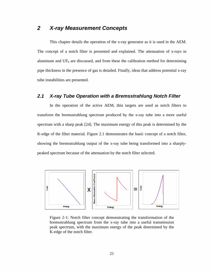
2.1 X-ray Tube Operation with a Bremsstrahlung Notch Filter
In the operation of the active AEM, thin targets are used as notch filters to
transform the bremsstrahlung spectrum produced by the x-ray tube into a more useful
spectrum with a sharp peak [24]. The maximum energy of this peak is determined by the
K-edge of the filter material. Figure 2.1 demonstrates the basic concept of a notch filter,
showing the bremsstrahlung output of the x-ray tube being transformed into a sharply-
peaked spectrum because of the attenuation by the notch filter selected.
Figure 2-1: Notch filter concept demonstrating the transformation of the bremsstrahlung spectrum from the x-ray tube into a useful transmission peak spectrum, with the maximum energy of the peak determined by the K-edge of the notch filter.
22
The x-ray tube is operated so that the energy it emits is slightly higher than the
K-absorption edge of the filter. A sharp peaked spectrum is emitted because the filter
absorbs radiation above the K-edge energy that corresponds to the binding energy of the
electrons in the K-shell of the atoms in the filter material.
One advantage of using an x-ray tube with notch filters is that it allows greater
flexibility in selecting transmission energies. Traditionally, when measurements were
performed with an isotopic source, the 22-keV silver x-ray from a decaying 109Cd source
was used to measure attenuation in the UF6 gas. There are not many choices available that
have both an optimum energy and a long enough half-life to be useful. With the notch
filter method, a wide range of transmission peak energies is available. However, there is a
trade-off between the attenuation in the gas and attenuation in the pipe, which is large for
such low energies. For the transmission measurement that determines the UF6 gas
density, the goal is to try to maximize the attenuation in the gas and minimize the
attenuation in the pipe. In order to do so, the AEM uses the highest energy possible that
will still give acceptable attenuation results in the gas. A silver filter is often used for this
purpose in normal operation of the AEM. For the pipe thickness measurement, however,
it is more important that the attenuation in the gas can be canceled out for two subsequent
transmission measurements, using the two-energy technique described previously.
Because this is a one-time measurement to characterize the pipe before the enrichment
measurements are performed, longer count times are acceptable, allowing lower energies
to be used. Because it is feasible to go to (slightly) lower energies than the silver notch
filter that has a K-edge at 25.5 keV, two filters can be chosen that have transmission
peaks at equal attenuation in the UF6 gas but different in the aluminum pipe. This
23
technique takes advantage of the fact that in the uranium L-edge region there are multiple
energies with equal attenuation coefficients.
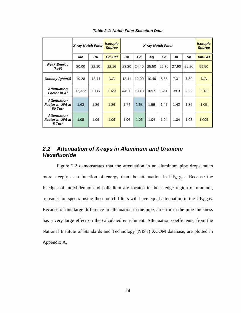
Table 2–1 shows a number of options for x-ray transmission notch filter materials
compared with two traditionally used radioisotopes. This table compares some of the data
previously presented [12] with an additional material, molybdenum. The table includes
K-edge energies of the various materials and attenuations in the 5-mm wall thickness
aluminum pipe. Also shown are attenuations in 10 cm of UF6 gas at 50 Torr (typical of a
downstream pipe header, where the AEM will be placed) and at 5 Torr (typical of an
upstream header before a pump). The K-edge of zirconium (18 keV) was also considered
because of its similar attenuation in UF6 to using a ruthenium notch filter, but the
attenuation in the aluminum pipe would have been unfeasibly large. It is important to
note the similar attenuation of molybdenum and palladium in the UF6 gas, both at 5 and
50 Torr. Because of these properties, molybdenum and palladium were selected as the
two notch filter target materials for the pipe thickness determination. All further work on
the two-energy pipe thickness method focuses on these two materials.
A silver filter was being considered for the final unattended transmission
measurements used to determine the enrichment [25]. Another possibility could have
been to use a palladium filter for the enrichment transmission measurement as well as one
of the two filters for the pipe attenuation determination. With less than a 1-keV difference
in the silver and palladium K-edges, this would have increased the absorption in the gas
by 5% at 50 Torr, but would have almost doubled the count time because of the higher
attenuation in the aluminum pipe. This may or may not be an acceptable compromise.
24
Table 2-1: Notch Filter Selection Data
X-ray Notch FilterIsotopic Source
X-ray Notch Filter Isotopic Source
Mo Ru Cd-109 Rh Pd Ag Cd In Sn Am-241
Peak Energy (keV)
20.00 22.10 22.16 23.20 24.40 25.50 26.70 27.90 29.20 59.50
Density (g/cm3) 10.28 12.44 N/A 12.41 12.00 10.49 8.65 7.31 7.30 N/A
Attenuation Factor in Al
12,322 1086 1029 445.6 198.3 109.5 62.1 39.3 26.2 2.13
Attenuation Factor in UF6 at
50 Torr 1.63 1.86 1.86 1.74 1.63 1.55 1.47 1.42 1.36 1.05
Attenuation Factor in UF6 at
5 Torr 1.05 1.06 1.06 1.06 1.05 1.04 1.04 1.04 1.03 1.005
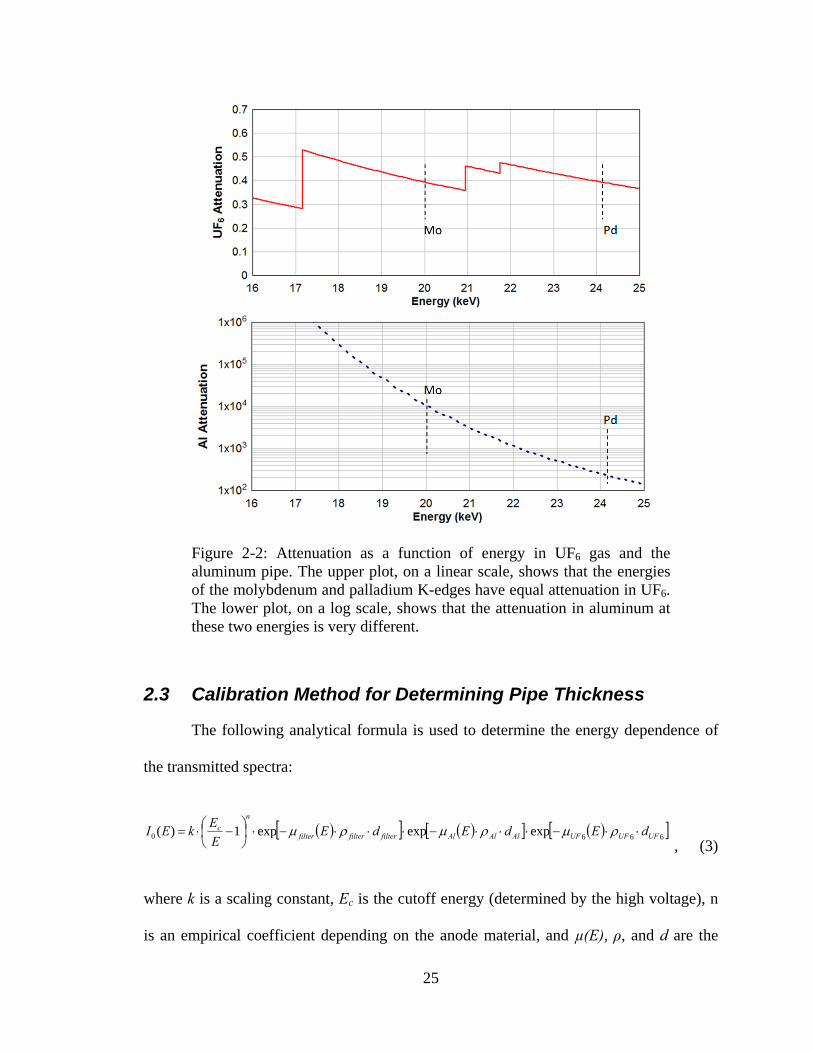
2.2 Attenuation of X-rays in Aluminum and Uranium Hexafluoride
Figure 2.2 demonstrates that the attenuation in an aluminum pipe drops much
more steeply as a function of energy than the attenuation in UF6 gas. Because the
K-edges of molybdenum and palladium are located in the L-edge region of uranium,
transmission spectra using these notch filters will have equal attenuation in the UF6 gas.
Because of this large difference in attenuation in the pipe, an error in the pipe thickness
has a very large effect on the calculated enrichment. Attenuation coefficients, from the
National Institute of Standards and Technology (NIST) XCOM database, are plotted in
Appendix A.
25
Figure 2-2: Attenuation as a function of energy in UF6 gas and the aluminum pipe. The upper plot, on a linear scale, shows that the energies of the molybdenum and palladium K-edges have equal attenuation in UF6. The lower plot, on a log scale, shows that the attenuation in aluminum at these two energies is very different.
2.3 Calibration Method for Determining Pipe Thickness
The following analytical formula is used to determine the energy dependence of
the transmitted spectra:
6660 expexpexp1)( UFUFUFAlAlAlfilterfilterfilter
n
c dEdEdEE
EkEI
, (3)
where k is a scaling constant, Ec is the cutoff energy (determined by the high voltage), n
is an empirical coefficient depending on the anode material, and µ(E), ρ, and d are the
26
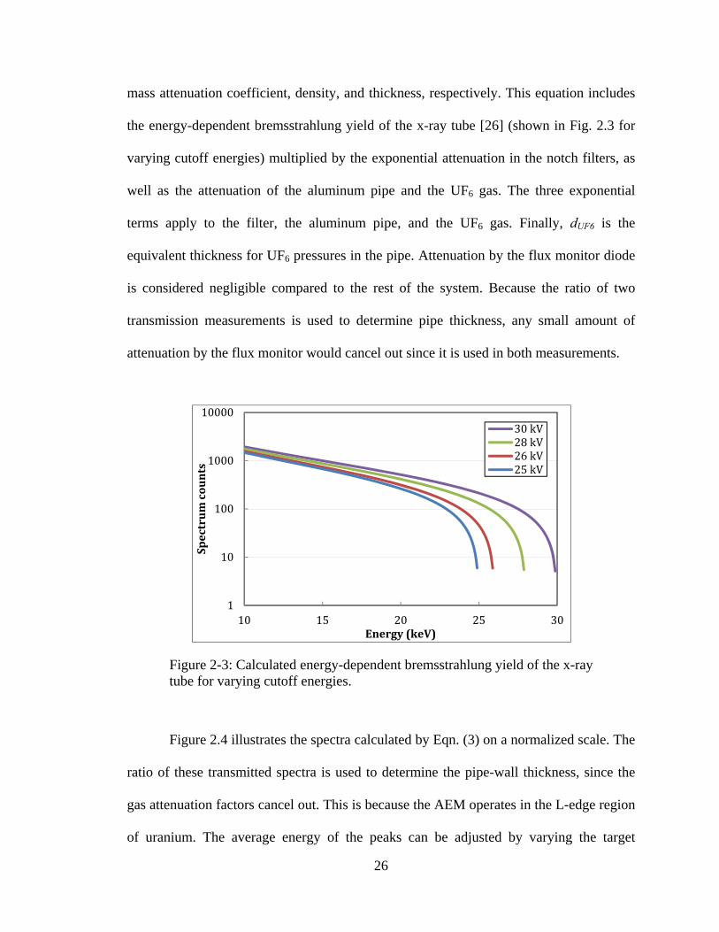
mass attenuation coefficient, density, and thickness, respectively. This equation includes
the energy-dependent bremsstrahlung yield of the x-ray tube [26] (shown in Fig. 2.3 for
varying cutoff energies) multiplied by the exponential attenuation in the notch filters, as
well as the attenuation of the aluminum pipe and the UF6 gas. The three exponential
terms apply to the filter, the aluminum pipe, and the UF6 gas. Finally, dUF6 is the
equivalent thickness for UF6 pressures in the pipe. Attenuation by the flux monitor diode
is considered negligible compared to the rest of the system. Because the ratio of two
transmission measurements is used to determine pipe thickness, any small amount of
attenuation by the flux monitor would cancel out since it is used in both measurements.
Figure 2-3: Calculated energy-dependent bremsstrahlung yield of the x-ray tube for varying cutoff energies.
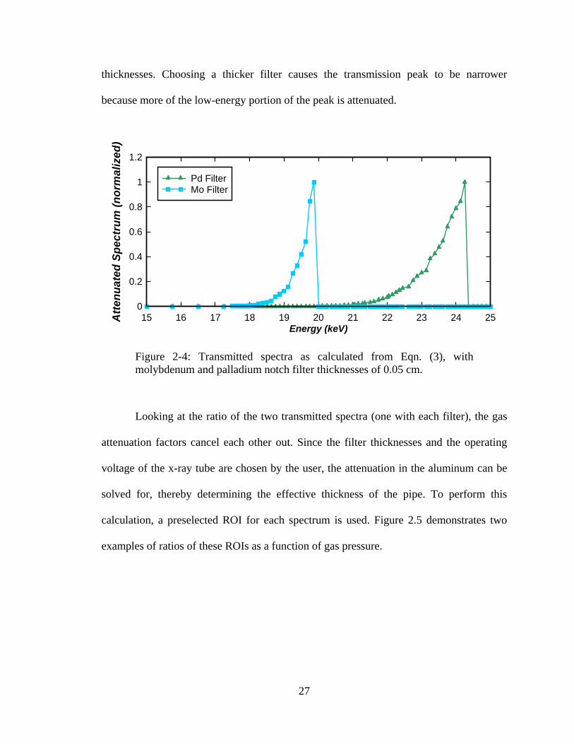
Figure 2.4 illustrates the spectra calculated by Eqn. (3) on a normalized scale. The
ratio of these transmitted spectra is used to determine the pipe-wall thickness, since the
gas attenuation factors cancel out. This is because the AEM operates in the L-edge region
of uranium. The average energy of the peaks can be adjusted by varying the target
1
10
100
1000
10000
10 15 20 25 30
Spectrumcounts
Energy(keV)
30kV28kV26kV25kV
27
thicknesses. Choosing a thicker filter causes the transmission peak to be narrower
because more of the low-energy portion of the peak is attenuated.
Figure 2-4: Transmitted spectra as calculated from Eqn. (3), with molybdenum and palladium notch filter thicknesses of 0.05 cm.
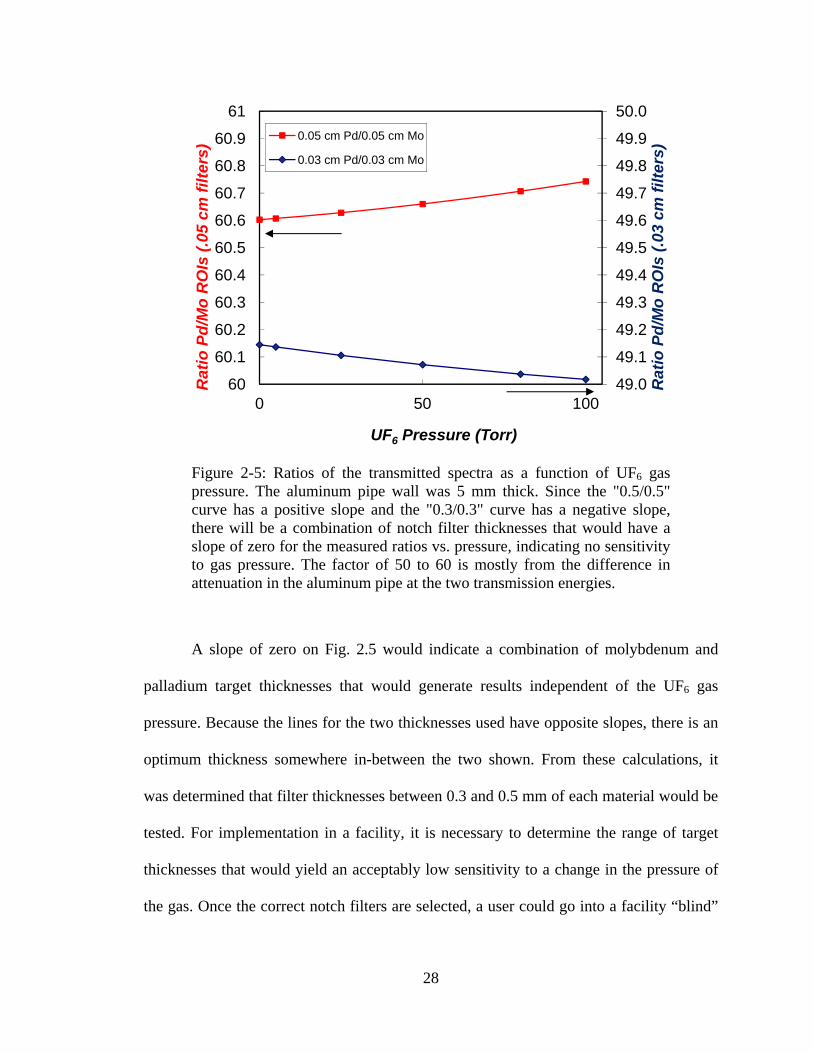
Looking at the ratio of the two transmitted spectra (one with each filter), the gas
attenuation factors cancel each other out. Since the filter thicknesses and the operating
voltage of the x-ray tube are chosen by the user, the attenuation in the aluminum can be
solved for, thereby determining the effective thickness of the pipe. To perform this
calculation, a preselected ROI for each spectrum is used. Figure 2.5 demonstrates two
examples of ratios of these ROIs as a function of gas pressure.
Energy (keV)
Att
enu
ated
Sp
ectr
um
(n
orm
aliz
ed)
15 16 17 18 19 20 21 22 23 24 250
0.2
0.4
0.6
0.8
1
1.2
Pd FilterMo Filter
28
Figure 2-5: Ratios of the transmitted spectra as a function of UF6 gas pressure. The aluminum pipe wall was 5 mm thick. Since the "0.5/0.5" curve has a positive slope and the "0.3/0.3" curve has a negative slope, there will be a combination of notch filter thicknesses that would have a slope of zero for the measured ratios vs. pressure, indicating no sensitivity to gas pressure. The factor of 50 to 60 is mostly from the difference in attenuation in the aluminum pipe at the two transmission energies.
A slope of zero on Fig. 2.5 would indicate a combination of molybdenum and
palladium target thicknesses that would generate results independent of the UF6 gas
pressure. Because the lines for the two thicknesses used have opposite slopes, there is an
optimum thickness somewhere in-between the two shown. From these calculations, it
was determined that filter thicknesses between 0.3 and 0.5 mm of each material would be
tested. For implementation in a facility, it is necessary to determine the range of target
thicknesses that would yield an acceptably low sensitivity to a change in the pressure of
the gas. Once the correct notch filters are selected, a user could go into a facility “blind”
49.0
49.1
49.2
49.3
49.4
49.5
49.6
49.7
49.8
49.9
50.0
60
60.1
60.2
60.3
60.4
60.5
60.6
60.7
60.8
60.9
61
0 50 100
Rat
io P
d/M
o R
OIs
(.0
3 cm
filt
ers)
Rat
io P
d/M
o R
OIs
(.0
5 cm
filt
ers)
UF6 Pressure (Torr)
0.05 cm Pd/0.05 cm Mo
0.03 cm Pd/0.03 cm Mo

29
and calibrate the AEM system on an operational system, without knowing the amount of
UF6 gas in the pipe.
2.4 Addressing Potential X-ray Tube Instability
An International Radiation Detectors Inc. (IRD Inc.) silicon flux monitor diode
[27] was explored for the measurement of the output of an x-ray tube used for active
transmission measurements on the pipe containing UF6 gas. The measured flux in the
diode can be used to correct for any instabilities in the x-ray tube or the high voltage
power supply. Temperature sensitivity and radiation hardness tests were performed to
determine the suitability of these diodes for use in the active implementation of the AEM.
Although these diodes have been extensively tested for radiation hardness in the
ultraviolet range, the enrichment monitor is operated in the 10- to 40-keV x-ray region.
Radiation hardness testing over this energy range was performed using the energy
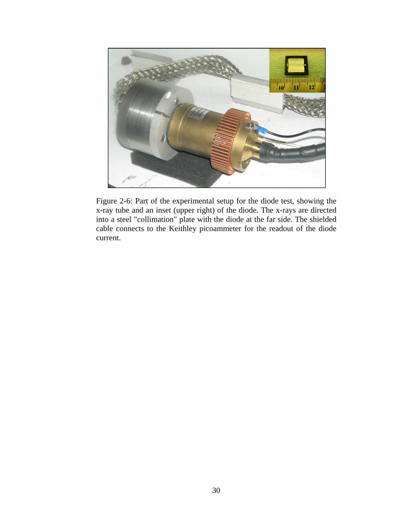
spectrum that would pass through the diode during normal operation. Figure 2.6 shows
the experimental setup used for this testing. The inset on the upper right is a picture of the
diode. Temperature sensitivity measurements were also performed with the diodes.
30
Figure 2-6: Part of the experimental setup for the diode test, showing the x-ray tube and an inset (upper right) of the diode. The x-rays are directed into a steel "collimation" plate with the diode at the far side. The shielded cable connects to the Keithley picoammeter for the readout of the diode current.
31
3 Experimental Implementation
The general experimental setup that is described in the following sections was used
as the basis for both the analytical calculations detailed in Chapter 4 and the experiments
performed to test the active AEM. A diagram of the passive AEM is also included here to
help distinguish the two systems.
3.1 Introduction
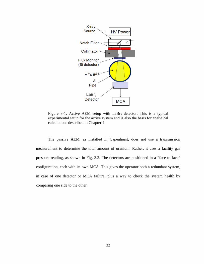
Figure 3.1 is a drawing of the active AEM, showing the x-ray tube and power
supply, notch filter, collimator, in-beam flux monitor (to correct for instabilities in the x-
ray output), pipe, and lanthanum bromide (LaBr3) detector with an MCA. The wall
thickness tests were performed with a LaBr3 detector, and the temperature and gas
pressure sensitivity tests were performed using a NaI detector.
32
Figure 3-1: Active AEM setup with LaBr3 detector. This is a typical experimental setup for the active system and is also the basis for analytical calculations described in Chapter 4.
The passive AEM, as installed in Capenhurst, does not use a transmission
measurement to determine the total amount of uranium. Rather, it uses a facility gas
pressure reading, as shown in Fig. 3.2. The detectors are positioned in a “face to face”
configuration, each with its own MCA. This gives the operator both a redundant system,
in case of one detector or MCA failure, plus a way to check the system health by
comparing one side to the other.

33
Figure 3-2: Passive AEM setup with NaI detectors. This is the way the passive system is currently configured, collecting data in Capenhurst. A pressure reading gives the total amount of uranium in the UF6 gas, and 186-keV counts give the amount of 235U.
3.2 X-ray Tube and Collimator
The x-ray generator used in the AEM is a Varian model VF-50J industrial tube
(see Appendix B for specifications) [28], with either a tungsten, silver, or palladium
anode. Of these, the tungsten anode tube is the most efficient. A greater amount of
incident radiation is converted to x-rays, rather than heat, due to its higher atomic number
[29]. The tube has a beryllium window and is powered by an XRM series Spellman high
voltage supply (described in Appendix B [30]). The operating current of the tube is about
150 µA, and the operating voltage is in the range of 35 kV. This x-ray tube was chosen
because it is capable of operating at beam currents much higher than needed for those
used in the AEM, suggesting a long operational lifetime. The x-ray tube is embedded in
the active measurement head (a steel fixture that gets mounted to the tungsten box around
the pipe), as shown in Fig. 3.3. An interlock switch, also shown in the figure of the active
34
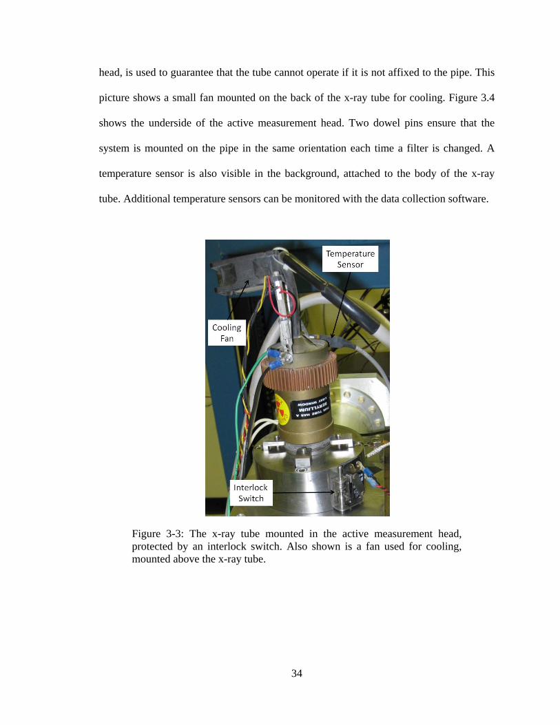
head, is used to guarantee that the tube cannot operate if it is not affixed to the pipe. This
picture shows a small fan mounted on the back of the x-ray tube for cooling. Figure 3.4
shows the underside of the active measurement head. Two dowel pins ensure that the
system is mounted on the pipe in the same orientation each time a filter is changed. A
temperature sensor is also visible in the background, attached to the body of the x-ray
tube. Additional temperature sensors can be monitored with the data collection software.
Figure 3-3: The x-ray tube mounted in the active measurement head, protected by an interlock switch. Also shown is a fan used for cooling, mounted above the x-ray tube.

35
Figure 3-4: Underside of the active head showing the flux monitor diode mounted in place as well as the dowel pins that are used to fix the orientation of the x-ray tube when notch filters are changed.
3.3 Notch Filters
Temperature sensitivity tests were performed using a silver notch filter, which
gives a transmission peak with the maximum energy at 25.5 keV. This filter was affixed
to the active head using an aluminum ring, placed directly in front of the x-ray tube. The
molybdenum and palladium notch filters for the pipe thickness experiment were
fabricated by cutting the 0.1-mm-thick sheets into 1.25” squares and attaching these
squares to aluminum rings that could be mounted directly above the flux monitor. This is
shown in Fig. 3.5. Filter thicknesses of 0.3 mm, 0.4 mm, and 0.5 mm were used for each
material; these were fabricated by stacking the required number of thicknesses of each
material on the aluminum rings.
36
Figure 3-5: Some of the molybdenum and palladium notch filters attached to their mounting rings.
The flux monitor and notch filter are mounted on the opposite side of the steel
fixture from the x-ray tube, as seen in Fig. 3.6. A hole collimator through the middle
ensures all of the beam hits the target and is directed through the flux monitor. The
positioning of the filter on the side of the collimator farthest from the x-ray tube allows
changing of the filters without affecting the position of the x-ray tube. This stability
allows spectra to be compared directly, without worrying about any geometrical errors
that may have been introduced when removing and reattaching the x-ray tube.
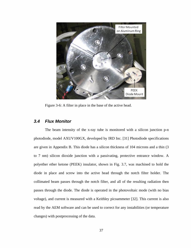
37
Figure 3-6: A filter in place in the base of the active head.
3.4 Flux Monitor
The beam intensity of the x-ray tube is monitored with a silicon junction p-n
photodiode, model AXUV100GX, developed by IRD Inc. [31] Photodiode specifications
are given in Appendix B. This diode has a silicon thickness of 104 microns and a thin (3
to 7 nm) silicon dioxide junction with a passivating, protective entrance window. A
polyether ether ketone (PEEK) insulator, shown in Fig. 3.7, was machined to hold the
diode in place and screw into the active head through the notch filter holder. The
collimated beam passes through the notch filter, and all of the resulting radiation then
passes through the diode. The diode is operated in the photovoltaic mode (with no bias
voltage), and current is measured with a Keithley picoammeter [32]. This current is also
read by the AEM software and can be used to correct for any instabilities (or temperature
changes) with postprocessing of the data.
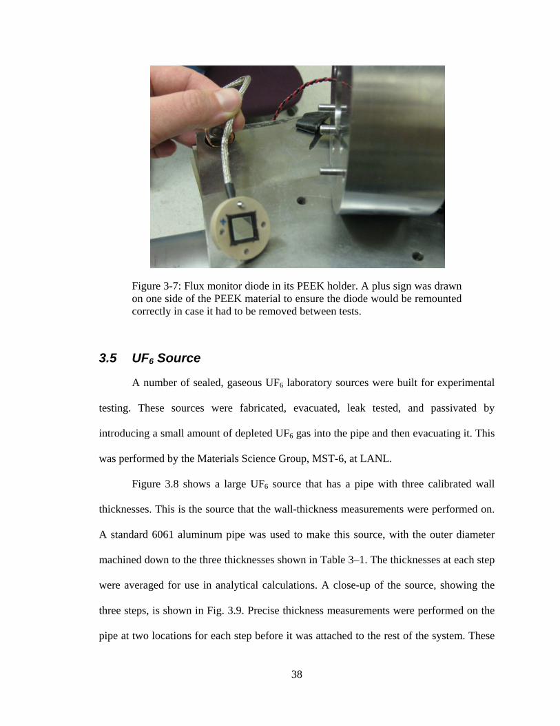
38
Figure 3-7: Flux monitor diode in its PEEK holder. A plus sign was drawn on one side of the PEEK material to ensure the diode would be remounted correctly in case it had to be removed between tests.
3.5 UF6 Source
A number of sealed, gaseous UF6 laboratory sources were built for experimental
testing. These sources were fabricated, evacuated, leak tested, and passivated by
introducing a small amount of depleted UF6 gas into the pipe and then evacuating it. This
was performed by the Materials Science Group, MST-6, at LANL.
Figure 3.8 shows a large UF6 source that has a pipe with three calibrated wall
thicknesses. This is the source that the wall-thickness measurements were performed on.
A standard 6061 aluminum pipe was used to make this source, with the outer diameter
machined down to the three thicknesses shown in Table 3–1. The thicknesses at each step
were averaged for use in analytical calculations. A close-up of the source, showing the
three steps, is shown in Fig. 3.9. Precise thickness measurements were performed on the
pipe at two locations for each step before it was attached to the rest of the system. These
39
data give us an idea of the error in the pipe thickness, which our density measurements
are very sensitive to.
This source allows for variable UF6 gas pressure (up to ~50 Torr), as well as
different enrichment levels. The manifold on the left end of the source has four
connections for bottles of UF6. To increase gas pressure in the pipe, the valve to the bottle
of the desired enrichment is opened. A high precision Baratron pressure gauge is used to
monitor the pressure in the pipe, and the valve is closed when the desired pressure is
reached. To lower gas pressure in the pipe, liquid nitrogen (LN2) cooling is used. A small
vessel, filled with LN2, is placed around the bottle that the UF6 is returned to. The valves
are then opened and the gas is cryogenically pumped back into the bottle.
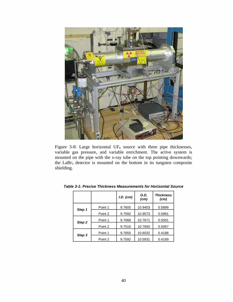
40
Figure 3-8: Large horizontal UF6 source with three pipe thicknesses, variable gas pressure, and variable enrichment. The active system is mounted on the pipe with the x-ray tube on the top pointing downwards; the LaBr3 detector is mounted on the bottom in its tungsten composite shielding.
Table 3-1: Precise Thickness Measurements for Horizontal Source
I.D. (cm) O.D. (cm)
Thickness (cm)
Step 1 Point 1 9.7605 10.9403 0.5899
Point 2 9.7592 10.9573 0.5991
Step 2 Point 1 9.7668 10.7671 0.5001
Point 2 9.7516 10.7650 0.5067
Step 3 Point 1 9.7655 10.6032 0.4188
Point 2 9.7592 10.5931 0.4169
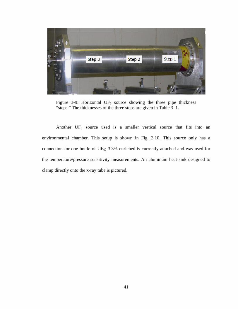
41
Figure 3-9: Horizontal UF6 source showing the three pipe thickness “steps.” The thicknesses of the three steps are given in Table 3–1.
Another UF6 source used is a smaller vertical source that fits into an
environmental chamber. This setup is shown in Fig. 3.10. This source only has a
connection for one bottle of UF6; 3.3% enriched is currently attached and was used for
the temperature/pressure sensitivity measurements. An aluminum heat sink designed to
clamp directly onto the x-ray tube is pictured.
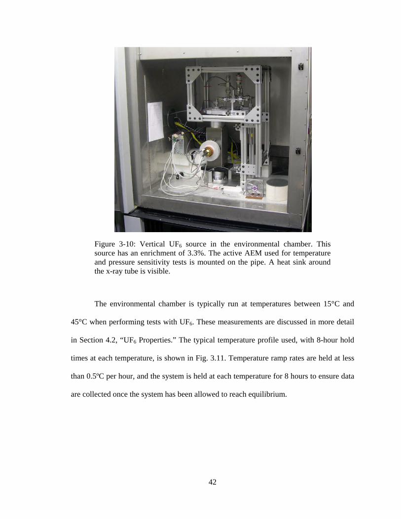
42
Figure 3-10: Vertical UF6 source in the environmental chamber. This source has an enrichment of 3.3%. The active AEM used for temperature and pressure sensitivity tests is mounted on the pipe. A heat sink around the x-ray tube is visible.
The environmental chamber is typically run at temperatures between 15°C and
45°C when performing tests with UF6. These measurements are discussed in more detail
in Section 4.2, “UF6 Properties.” The typical temperature profile used, with 8-hour hold
times at each temperature, is shown in Fig. 3.11. Temperature ramp rates are held at less
than 0.5ºC per hour, and the system is held at each temperature for 8 hours to ensure data
are collected once the system has been allowed to reach equilibrium.
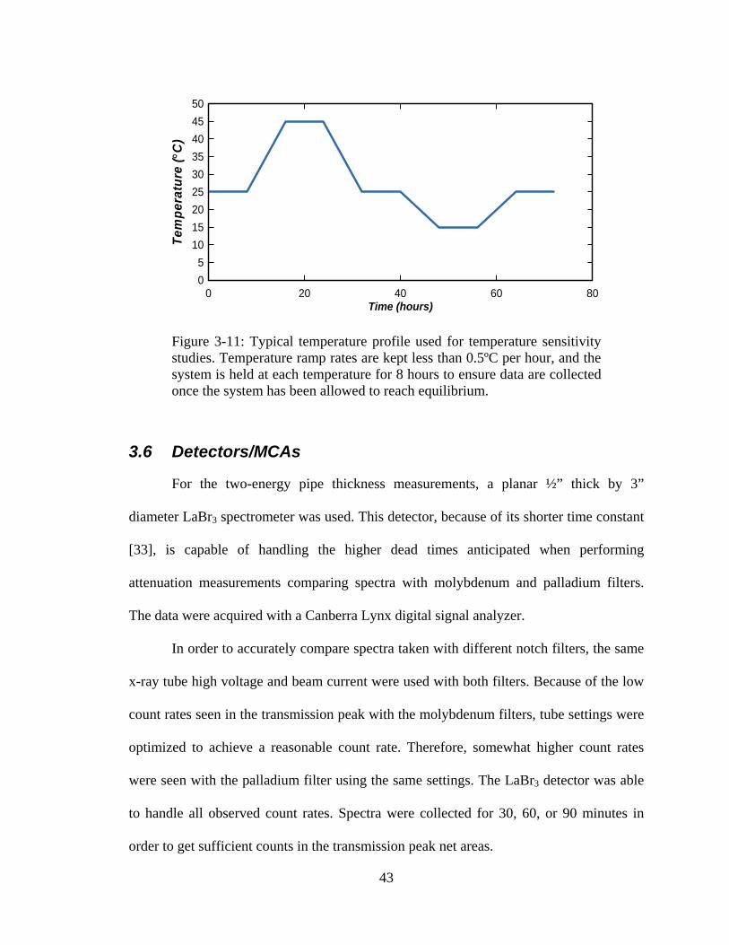
43
Figure 3-11: Typical temperature profile used for temperature sensitivity studies. Temperature ramp rates are kept less than 0.5ºC per hour, and the system is held at each temperature for 8 hours to ensure data are collected once the system has been allowed to reach equilibrium.
3.6 Detectors/MCAs
For the two-energy pipe thickness measurements, a planar ½” thick by 3”
diameter LaBr3 spectrometer was used. This detector, because of its shorter time constant
[33], is capable of handling the higher dead times anticipated when performing
attenuation measurements comparing spectra with molybdenum and palladium filters.
The data were acquired with a Canberra Lynx digital signal analyzer.
In order to accurately compare spectra taken with different notch filters, the same
x-ray tube high voltage and beam current were used with both filters. Because of the low
count rates seen in the transmission peak with the molybdenum filters, tube settings were
optimized to achieve a reasonable count rate. Therefore, somewhat higher count rates
were seen with the palladium filter using the same settings. The LaBr3 detector was able
to handle all observed count rates. Spectra were collected for 30, 60, or 90 minutes in
order to get sufficient counts in the transmission peak net areas.
Time (hours)
Tem
per
atu
re (C
)
0 20 40 60 800
5
10
15
20
25
30
35
40
45
50

44
For the temperature and pressure sensitivity measurements, NaI(Tl) detectors
were used. These are the most commonly used detectors in enrichment monitoring
because of their low cost, good efficiency, and sufficient resolution for the task. Table 3–
2 compares some of the significant characteristics of NaI and LaBr3 detectors [34].
Table 3-2: Comparison between LaBr3 and NaI Scintillators
An ORTEC DigiDART MCA was used with the NaI detector for the temperature
and gas pressure sensitivity measurements [35].
Density (g/cm3)
Resolution (%) 122 keV
Resolution (%) 662 keV
Light yield (photons/keV)
Decay time (ns)
NaI:Tl 3.67 8.0 6.5 39 16
LaBr3:Ce 5.1 6.0 2.8 65 250
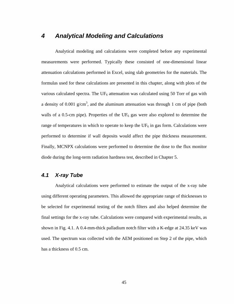
45
4 Analytical Modeling and Calculations
Analytical modeling and calculations were completed before any experimental
measurements were performed. Typically these consisted of one-dimensional linear
attenuation calculations performed in Excel, using slab geometries for the materials. The
formulas used for these calculations are presented in this chapter, along with plots of the
various calculated spectra. The UF6 attenuation was calculated using 50 Torr of gas with
a density of 0.001 g/cm3, and the aluminum attenuation was through 1 cm of pipe (both
walls of a 0.5-cm pipe). Properties of the UF6 gas were also explored to determine the
range of temperatures in which to operate to keep the UF6 in gas form. Calculations were
performed to determine if wall deposits would affect the pipe thickness measurement.
Finally, MCNPX calculations were performed to determine the dose to the flux monitor
diode during the long-term radiation hardness test, described in Chapter 5.
4.1 X-ray Tube
Analytical calculations were performed to estimate the output of the x-ray tube
using different operating parameters. This allowed the appropriate range of thicknesses to
be selected for experimental testing of the notch filters and also helped determine the
final settings for the x-ray tube. Calculations were compared with experimental results, as
shown in Fig. 4.1. A 0.4-mm-thick palladium notch filter with a K-edge at 24.35 keV was
used. The spectrum was collected with the AEM positioned on Step 2 of the pipe, which
has a thickness of 0.5 cm.

46
Figure 4-1: Comparison between a calculated and measured spectrum. A 0.4-mm-thick palladium notch filter with a K-edge at 24.35 keV was used, and there was 50 Torr of gas in the pipe.
The most noticeable difference between the measured and calculated spectra is
the width of the peaks, which is affected by the detector resolution in the actual data.
Also evident in the measured spectrum is the lanthanum x-ray peak that comes from
internal radioactivity of the LaBr3 detector, which does not show up in calculations that
only display radiation incident on the detector.
4.1.1 Generated and Transmitted Spectra
The Varian x-ray tubes that are used for the active portion of the AEM have a
maximum operating voltage of 50 kV. We generally try to operate these tubes at a much
lower power than they are rated for so they will last a long time in an unattended
monitoring situation. One of these tubes was operated in the laboratory at a voltage of
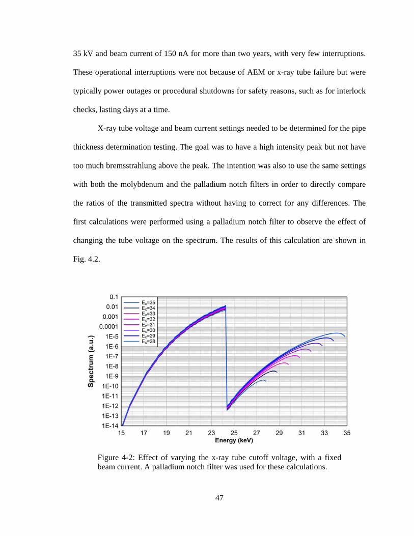
47
35 kV and beam current of 150 nA for more than two years, with very few interruptions.
These operational interruptions were not because of AEM or x-ray tube failure but were
typically power outages or procedural shutdowns for safety reasons, such as for interlock
checks, lasting days at a time.
X-ray tube voltage and beam current settings needed to be determined for the pipe
thickness determination testing. The goal was to have a high intensity peak but not have
too much bremsstrahlung above the peak. The intention was also to use the same settings
with both the molybdenum and the palladium notch filters in order to directly compare
the ratios of the transmitted spectra without having to correct for any differences. The
first calculations were performed using a palladium notch filter to observe the effect of
changing the tube voltage on the spectrum. The results of this calculation are shown in
Fig. 4.2.
Figure 4-2: Effect of varying the x-ray tube cutoff voltage, with a fixed beam current. A palladium notch filter was used for these calculations.

48
The calculations showed that while increasing the cutoff voltage of the tube does
increase the intensity of the peak, it does not change its width. However, there is a
tradeoff because making the cutoff voltage too high allows more and more of the
bremsstrahlung above the K-edge of the notch filters to leak through, as was shown in the
above figure. For this reason, a cutoff voltage of 30 kV was chosen, and the beam current
was increased from the typical setting of 100 µA to 160 µA. Increasing the beam current
simply increases the flux from the tube without changing the shape of the spectrum.
4.1.2 Issues with Analytical Model
The following analytical formula was used to determine the transmitted spectra,
as detailed in equation 3 from Section 2.3:
The empirical coefficient describing the anode material n was determined by
extrapolation from the data in McCall’s paper (shown in Table 4–1), which came from
Jakschik [26].
Table 4-1: X-ray Generator—Anode Material Coefficients
Element Z n
Beryllium 4 1.28
Aluminum 13 1.23
Copper 29 1.08
Silver 47 0.96
Gold 79 0.91
0 6 6 6( ) 1 exp exp expn
cfilter filter filter Al Al Al UF UF UF
EI E k E d E d E d
E
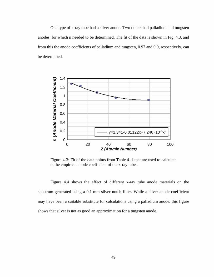
49
One type of x-ray tube had a silver anode. Two others had palladium and tungsten
anodes, for which n needed to be determined. The fit of the data is shown in Fig. 4.3, and
from this the anode coefficients of palladium and tungsten, 0.97 and 0.9, respectively, can
be determined.
Figure 4-3: Fit of the data points from Table 4–1 that are used to calculate n, the empirical anode coefficient of the x-ray tubes.
Figure 4.4 shows the effect of different x-ray tube anode materials on the
spectrum generated using a 0.1-mm silver notch filter. While a silver anode coefficient
may have been a suitable substitute for calculations using a palladium anode, this figure
shows that silver is not as good an approximation for a tungsten anode.
Z (Atomic Number)
n (
An
od
e M
ater
ial C
oef
fici
ent)
0 20 40 60 80 1000
0.2
0.4
0.6
0.8
1
1.2
1.4
y=1.341-0.01122x+7.24610-5x2

50
Figure 4-4: The effect of different x-ray tube anode materials on the spectrum generated using a 0.1-mm silver notch filter. This figure shows that although silver may be a good approximation for a palladium anode, it cannot substitute in calculations for a tungsten anode.
Also, note that I(E) is the calculation of the beam that hits the detector, but it is
not necessarily what the detector measures. Since the two transmission peaks generated
using the notch filters are both below 25 keV, detector efficiency in either the LaBr3 or
the NaI should not cause any differences between the two measured spectra. However,
the resolution of the detector will affect the shape of the spectrum measured. For this
reason, calculated spectra appear to have a sharp drop in intensity at the K-edge of the
notch filter used, whereas measured spectra are broadened from the detector resolution.
0
50
100
150
200
250
10 15 20 25 30 35 40
Sp
ectr
um
(a.
u.)
E (keV)
n=0.895 (W anode)
n=0.96 (Ag anode)
n=0.973 (Pd anode)
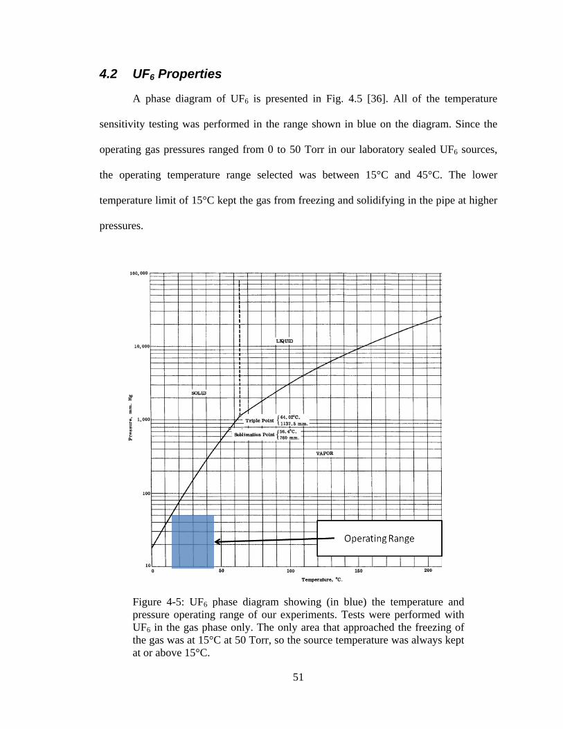
51
4.2 UF6 Properties
A phase diagram of UF6 is presented in Fig. 4.5 [36]. All of the temperature
sensitivity testing was performed in the range shown in blue on the diagram. Since the
operating gas pressures ranged from 0 to 50 Torr in our laboratory sealed UF6 sources,
the operating temperature range selected was between 15°C and 45°C. The lower
temperature limit of 15°C kept the gas from freezing and solidifying in the pipe at higher
pressures.
Figure 4-5: UF6 phase diagram showing (in blue) the temperature and pressure operating range of our experiments. Tests were performed with UF6 in the gas phase only. The only area that approached the freezing of the gas was at 15°C at 50 Torr, so the source temperature was always kept at or above 15°C.
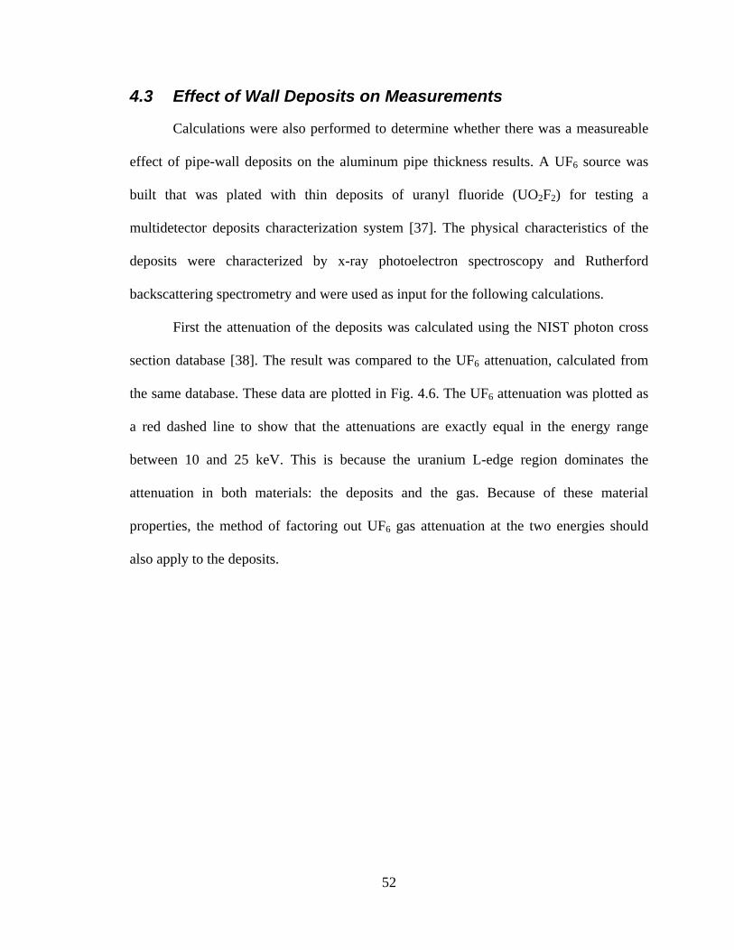
52
4.3 Effect of Wall Deposits on Measurements
Calculations were also performed to determine whether there was a measureable
effect of pipe-wall deposits on the aluminum pipe thickness results. A UF6 source was
built that was plated with thin deposits of uranyl fluoride (UO2F2) for testing a
multidetector deposits characterization system [37]. The physical characteristics of the
deposits were characterized by x-ray photoelectron spectroscopy and Rutherford
backscattering spectrometry and were used as input for the following calculations.
First the attenuation of the deposits was calculated using the NIST photon cross
section database [38]. The result was compared to the UF6 attenuation, calculated from
the same database. These data are plotted in Fig. 4.6. The UF6 attenuation was plotted as
a red dashed line to show that the attenuations are exactly equal in the energy range
between 10 and 25 keV. This is because the uranium L-edge region dominates the
attenuation in both materials: the deposits and the gas. Because of these material
properties, the method of factoring out UF6 gas attenuation at the two energies should
also apply to the deposits.
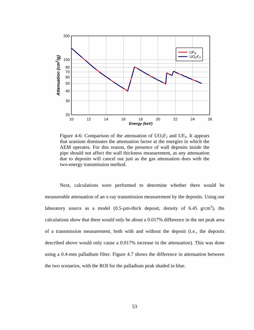
53
Figure 4-6: Comparison of the attenuation of UO2F2 and UF6. It appears that uranium dominates the attenuation factor at the energies in which the AEM operates. For this reason, the presence of wall deposits inside the pipe should not affect the wall thickness measurement, as any attenuation due to deposits will cancel out just as the gas attenuation does with the two-energy transmission method.
Next, calculations were performed to determine whether there would be
measureable attenuation of an x-ray transmission measurement by the deposits. Using our
laboratory source as a model (0.5-µm-thick deposit, density of 6.45 g/cm3), the
calculations show that there would only be about a 0.017% difference in the net peak area
of a transmission measurement, both with and without the deposit (i.e., the deposits
described above would only cause a 0.017% increase in the attenuation). This was done
using a 0.4-mm palladium filter. Figure 4.7 shows the difference in attenuation between
the two scenarios, with the ROI for the palladium peak shaded in blue.
Energy (keV)
Att
enu
atio
n (
cm2 /g
)
10 12 14 16 18 20 22 24 2620
30
40
50
607080
100
200
UF6UO2F2
54
Figure 4-7: Difference in attenuation between the pipe with and without deposits, with the ROI for the palladium peak shaded blue.
The effect was even smaller with a molybdenum filter because those generated
peaks had lower net count rates due to the higher pipe attenuation. Since the statistical
uncertainty in the net area with the palladium filter was about 0.08% (for a 1,800-s
measurement), there was no significant measureable attenuation by the deposits.
Moreover, once the one-time thickness measurement had been completed, we switch to
another filter with a higher transmission energy, such as silver, for the unattended
enrichment monitoring. A transmission peak generated by a silver notch filter would be
even less attenuated by uranium deposits than the palladium, since the peak would be at a
higher energy (K-edge at 25.5 keV).
0.00%
0.01%
0.02%
0.03%
0.04%
0.05%
15 17 19 21 23 25
PercentDifferenceinAttenuation
Energy(keV)
55
On the other hand, if there is a known enrichment for calibrating the system, such
as from a mass spectrometer measurement, deposits in the pipe can be corrected for.
Since the deposits should not change significantly over the monitoring time (as long as
the pipe is not brand new when monitoring is begun), this correction should remain valid.
Even if the deposits are a different enrichment than the UF6 gas, the two-energy pipe
thickness determination method should work because attenuation by the uranium is what
cancels, and it is independent of enrichment. The intent of the AEM is not to quantify the
deposits but rather to determine the portion of the 186-keV count rate that comes from
deposits (of any enrichment) to enable a correct enrichment determination over time.
4.4 Flux Monitor Diode
The following analytical formula is used to describe the energy spectrum seen by
the flux monitor diode:
AgAgAg
n
c dEE
EkI
)(exp1 . (4)
The intensity of the energy spectrum I is the bremsstrahlung yield of the tube [26]
multiplied by the attenuation in the silver notch filter. The terms µAg, ρAg, and dAg are the
mass attenuation coefficient, density, and thickness of the silver notch filter, respectively.
The cutoff voltage of the tube, Ec, was set to 40 kV. This is a typical voltage setting that
could be used in operation in a GCEP. The beam current can then be increased to raise
the flux at the diode to simulate very long operating times. Figure 4.8 shows the
calculated spectrum that is generated by the silver attenuated x-ray tube beam. A
0.1-mm-thick silver notch filter was used for the hardness testing to reduce the
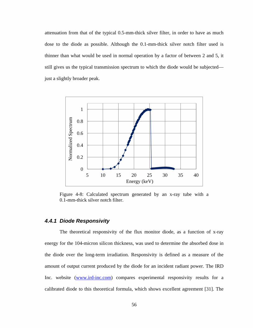
56
attenuation from that of the typical 0.5-mm-thick silver filter, in order to have as much
dose to the diode as possible. Although the 0.1-mm-thick silver notch filter used is
thinner than what would be used in normal operation by a factor of between 2 and 5, it
still gives us the typical transmission spectrum to which the diode would be subjected—
just a slightly broader peak.
Figure 4-8: Calculated spectrum generated by an x-ray tube with a 0.1-mm-thick silver notch filter.
4.4.1 Diode Responsivity
The theoretical responsivity of the flux monitor diode, as a function of x-ray
energy for the 104-micron silicon thickness, was used to determine the absorbed dose in
the diode over the long-term irradiation. Responsivity is defined as a measure of the
amount of output current produced by the diode for an incident radiant power. The IRD
Inc. website (www.ird-inc.com) compares experimental responsivity results for a
calibrated diode to this theoretical formula, which shows excellent agreement [31]. The
0
0.2
0.4
0.6
0.8
1
5 10 15 20 25 30 35 40
Nor
mal
ized
Spe
ctru
m
Energy (keV)
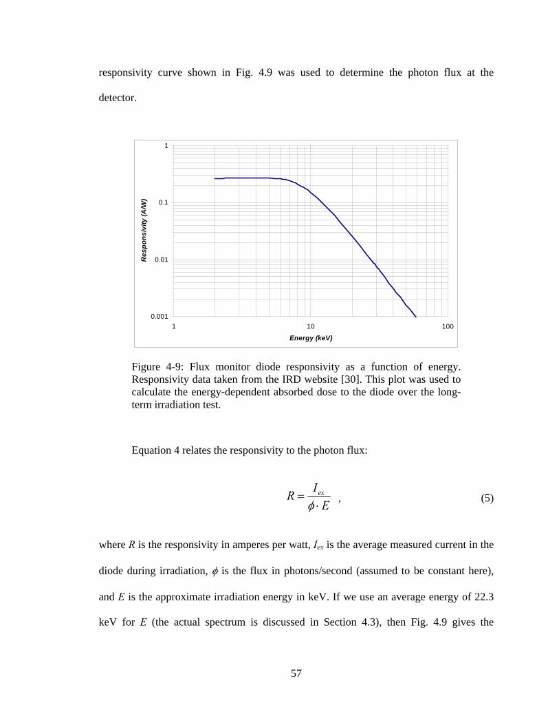
57
responsivity curve shown in Fig. 4.9 was used to determine the photon flux at the
detector.
Figure 4-9: Flux monitor diode responsivity as a function of energy. Responsivity data taken from the IRD website [30]. This plot was used to calculate the energy-dependent absorbed dose to the diode over the long-term irradiation test.
Equation 4 relates the responsivity to the photon flux:
E
IR ex
, (5)
where R is the responsivity in amperes per watt, Iex is the average measured current in the
diode during irradiation, is the flux in photons/second (assumed to be constant here),
and E is the approximate irradiation energy in keV. If we use an average energy of 22.3
keV for E (the actual spectrum is discussed in Section 4.3), then Fig. 4.9 gives the
0.001
0.01
0.1
1
1 10 100
Energy (keV)
Re
sp
on
siv
ity
(A
/W)
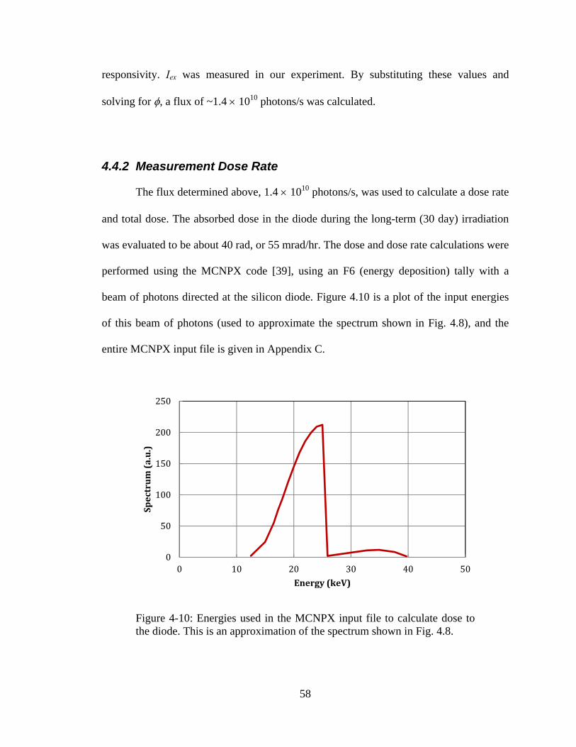
58
responsivity. Iex was measured in our experiment. By substituting these values and
solving for , a flux of ~1.4 1010 photons/s was calculated.
4.4.2 Measurement Dose Rate
The flux determined above, 1.4 1010 photons/s, was used to calculate a dose rate
and total dose. The absorbed dose in the diode during the long-term (30 day) irradiation
was evaluated to be about 40 rad, or 55 mrad/hr. The dose and dose rate calculations were
performed using the MCNPX code [39], using an F6 (energy deposition) tally with a
beam of photons directed at the silicon diode. Figure 4.10 is a plot of the input energies
of this beam of photons (used to approximate the spectrum shown in Fig. 4.8), and the
entire MCNPX input file is given in Appendix C.
Figure 4-10: Energies used in the MCNPX input file to calculate dose to the diode. This is an approximation of the spectrum shown in Fig. 4.8.
0
50
100
150
200
250
0 10 20 30 40 50
Spectrum(a.u.)
Energy(keV)

59
The spectrum counts are in arbitrary units; MCNPX normalizes the input
intensities before running. These MCNPX calculations, using the energy responsivity
curve provided by the diode manufacturer, determined that the absorbed dose in the diode
during the long-term irradiation was about 40 rad, or 55 mrad/hr. Section 5.1, “Flux
Monitor Diode Measurements,” will show the results of the long-term diode test,
demonstrating that the diode continued to operate in the desired manner after receiving a
dose of 40 rad.
60
5 Experimental Measurements
Experimental measurements form the basis of this dissertation, as the purpose is
to operate the AEM in the field as accurately as possible. First, radiation hardness
measurements were performed on the flux monitor diode to test whether it could
withstand the long-term x-ray radiation used in the AEM. Next the dual-energy method
was evaluated. These dual-energy measurements comprised the largest portion of the
experimental work in this dissertation, as close to 100 individual transmission
measurements were performed to optimize the notch filter ratio and x-ray tube settings.
Temperature and pressure sensitivity tests were performed with both the active and
passive AEM systems. Finally, some details of initial measurements from the URENCO
Capenhurst field trial have been presented.
5.1 Flux Monitor Diode Measurements
A long-term measurement was performed at a high flux, simulating more than 80
years of operation. No significant degradation was seen during this time. Fluctuations
were found to be within the 0.1% operationally acceptable error range. After irradiation,
an I-V characterization showed a temporary irradiation effect that decayed over time.
This effect was small because the diode was operated without external bias.
5.1.1 Long-term Irradiation Measurement
The diode was irradiated at a tube voltage of 40 kV and a beam current of 1 mA.
With the 0.1-mm-thick silver filter in place, an average current of 3,491 nA was induced
in the diode. The average diode current was measured with a Keithley picoammeter,
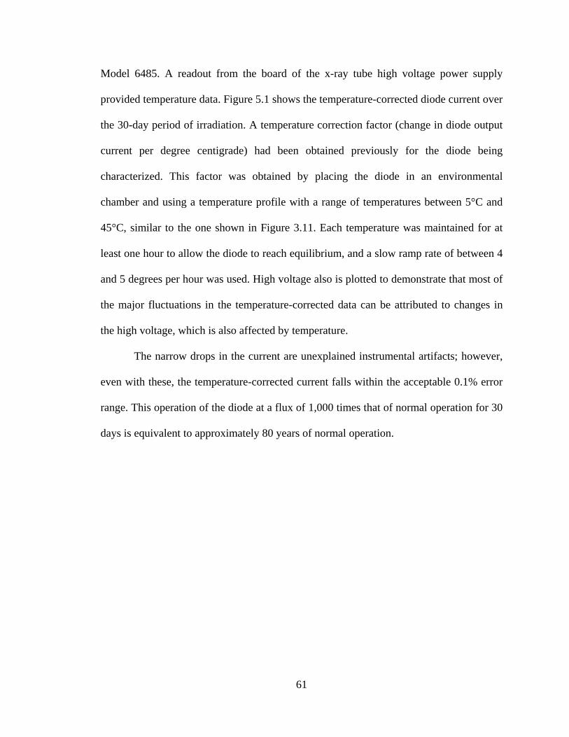
61
Model 6485. A readout from the board of the x-ray tube high voltage power supply
provided temperature data. Figure 5.1 shows the temperature-corrected diode current over
the 30-day period of irradiation. A temperature correction factor (change in diode output
current per degree centigrade) had been obtained previously for the diode being
characterized. This factor was obtained by placing the diode in an environmental
chamber and using a temperature profile with a range of temperatures between 5°C and
45°C, similar to the one shown in Figure 3.11. Each temperature was maintained for at
least one hour to allow the diode to reach equilibrium, and a slow ramp rate of between 4
and 5 degrees per hour was used. High voltage also is plotted to demonstrate that most of
the major fluctuations in the temperature-corrected data can be attributed to changes in
the high voltage, which is also affected by temperature.
The narrow drops in the current are unexplained instrumental artifacts; however,
even with these, the temperature-corrected current falls within the acceptable 0.1% error
range. This operation of the diode at a flux of 1,000 times that of normal operation for 30
days is equivalent to approximately 80 years of normal operation.
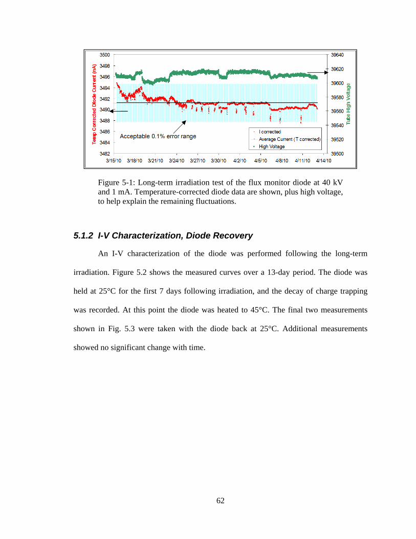
62
Figure 5-1: Long-term irradiation test of the flux monitor diode at 40 kV and 1 mA. Temperature-corrected diode data are shown, plus high voltage, to help explain the remaining fluctuations.
5.1.2 I-V Characterization, Diode Recovery
An I-V characterization of the diode was performed following the long-term
irradiation. Figure 5.2 shows the measured curves over a 13-day period. The diode was
held at 25°C for the first 7 days following irradiation, and the decay of charge trapping
was recorded. At this point the diode was heated to 45°C. The final two measurements
shown in Fig. 5.3 were taken with the diode back at 25°C. Additional measurements
showed no significant change with time.
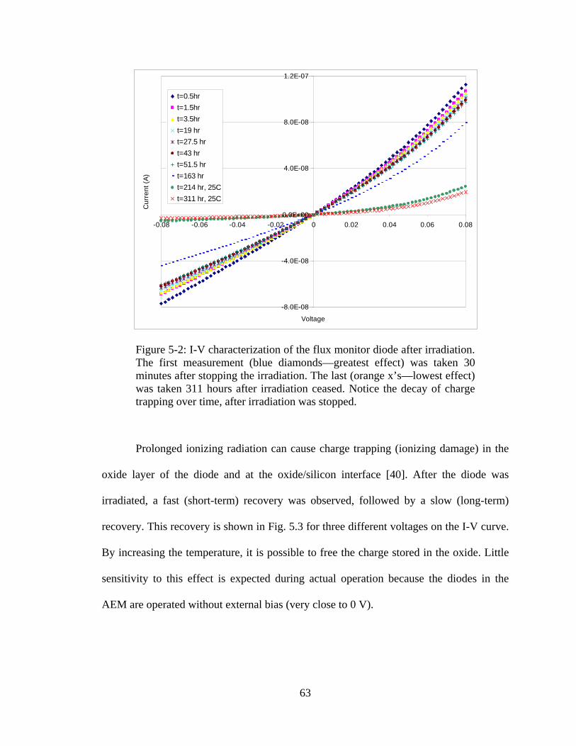
63
Figure 5-2: I-V characterization of the flux monitor diode after irradiation. The first measurement (blue diamonds—greatest effect) was taken 30 minutes after stopping the irradiation. The last (orange x’s—lowest effect) was taken 311 hours after irradiation ceased. Notice the decay of charge trapping over time, after irradiation was stopped.
Prolonged ionizing radiation can cause charge trapping (ionizing damage) in the
oxide layer of the diode and at the oxide/silicon interface [40]. After the diode was
irradiated, a fast (short-term) recovery was observed, followed by a slow (long-term)
recovery. This recovery is shown in Fig. 5.3 for three different voltages on the I-V curve.
By increasing the temperature, it is possible to free the charge stored in the oxide. Little
sensitivity to this effect is expected during actual operation because the diodes in the
AEM are operated without external bias (very close to 0 V).
-8.0E-08
-4.0E-08
0.0E+00
4.0E-08
8.0E-08
1.2E-07
-0.08 -0.06 -0.04 -0.02 0 0.02 0.04 0.06 0.08
Voltage
Cu
rre
nt
(A)
t=0.5hr
t=1.5hr
t=3.5hr
t=19 hr
t=27.5 hr
t=43 hr
t=51.5 hr
t=163 hr
t=214 hr, 25C
t=311 hr, 25C
64
Figure 5-3: Observed recovery of the flux monitor diode after the long-term irradiation test for three voltages on the I-V curve shown in Fig. 5.2. Short- and long-term recovery of the diode from charge trapping is shown.
No permanent damage to the diode appears to have been done by any of the long-
term measurements. Small fluctuations of the measured current were seen, but these can
be explained by temperature changes in the room and fluctuations in the x-ray tube high
voltage. After an equivalent of 80 years of standard operation, the diode still continued to
function as needed for use in the active AEM.
No permanent damage done to the silicon diode was seen when testing with x-ray
energies that are useful for performing transmission-based enrichment measurements in a
GCEP. It appears that a temporary charge-trapping effect may exist that was caused by
irradiation of the diodes with x-rays in the 10- to 40-keV region. However, the diode
received an absorbed dose of about 40 rad with no observed degradation in its operation.
Therefore, these flux monitors will be useful tools for stabilizing x-ray tubes during the
long durations of possibly unattended monitoring in a facility.
Time (hours)
Cu
rren
t (n
A)
0 20 40 60 80 100 120 140 160 1801
2
3
4
5
6
7
I @ 0.006 VI @ 0.004 VI @ 0.002 V
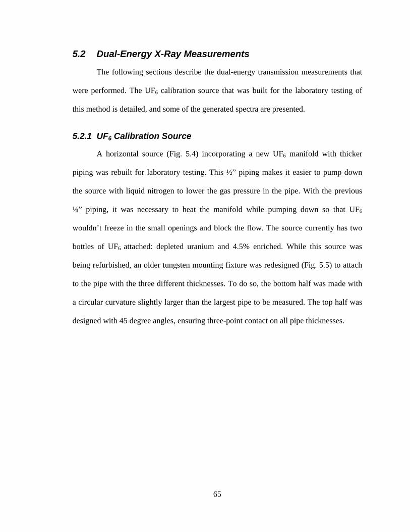
65
5.2 Dual-Energy X-Ray Measurements
The following sections describe the dual-energy transmission measurements that
were performed. The UF6 calibration source that was built for the laboratory testing of
this method is detailed, and some of the generated spectra are presented.
5.2.1 UF6 Calibration Source
A horizontal source (Fig. 5.4) incorporating a new UF6 manifold with thicker
piping was rebuilt for laboratory testing. This ½” piping makes it easier to pump down
the source with liquid nitrogen to lower the gas pressure in the pipe. With the previous
¼” piping, it was necessary to heat the manifold while pumping down so that UF6
wouldn’t freeze in the small openings and block the flow. The source currently has two
bottles of UF6 attached: depleted uranium and 4.5% enriched. While this source was
being refurbished, an older tungsten mounting fixture was redesigned (Fig. 5.5) to attach
to the pipe with the three different thicknesses. To do so, the bottom half was made with
a circular curvature slightly larger than the largest pipe to be measured. The top half was
designed with 45 degree angles, ensuring three-point contact on all pipe thicknesses.
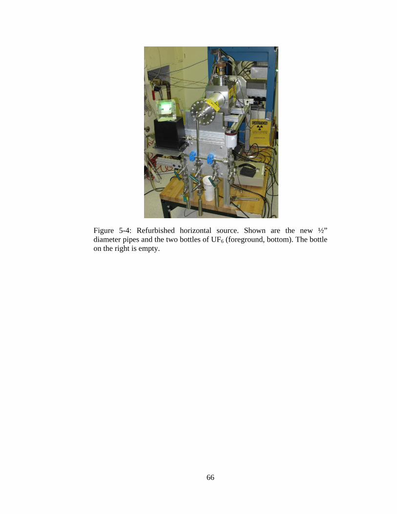
66
Figure 5-4: Refurbished horizontal source. Shown are the new ½” diameter pipes and the two bottles of UF6 (foreground, bottom). The bottle on the right is empty.
67
Figure 5-5: Redesigned mounting/shielding box, showing ability to mount on different pipe thicknesses
5.2.2 Transmission Measurements
A number of measurements were performed to test the technique for determining
attenuation, including the following variables:
Pipe thickness
Notch filter thickness
UF6 gas pressure
While the source was disassembled it was cleaned, and precise wall-thickness
measurements were performed. Thicknesses were determined at two points on each step
of the pipe. The measurements were performed at the ends of each step. The data, shown
in Table 3–1, give us a better idea of the error in the pipe thickness, which our density
measurements are very sensitive to.
68
More than 90 measurements were taken to acquire the spectra needed to optimize
the combination of molybdenum and palladium notch filters. Both molybdenum and
palladium filters of 0.3-mm, 0.4-mm, and 0.5-mm thicknesses were used. First, empty
pipe measurements were taken and spectra were collected with each of the six filters on
each step of the pipe. The UF6 (4.5% enriched) gas pressure was then increased in steps
up to 50 Torr, which is the limit of the UF6 contained in this closed system. Spectra were
collected for either 1,800 or 3,600 seconds, depending on the count rate in the
transmission peak. The transmission of the peak generated by the molybdenum notch
filter was much lower than the peak with palladium because there was much higher
attenuation in the aluminum pipe for the 20-keV molybdenum peak than for the 24.3-keV
palladium peak.
5.2.3 Gamma-ray Spectra
A ½” thick by 3” diameter LaBr3 spectrometer was used for the pipe thickness
measurements. This detector is capable of handling the higher dead times that were
anticipated when performing attenuation measurements comparing spectra with
molybdenum and palladium filters. The MCA was a Canberra Lynx digital signal
analyzer, to further help with the possible high dead times that might have been
encountered. A screen shot of Canberra’s Lynx data acquisition interface is shown in
Fig. 5.6.
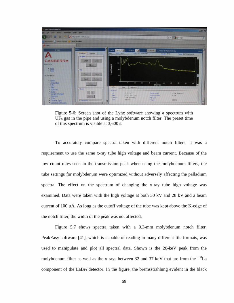
69
Figure 5-6: Screen shot of the Lynx software showing a spectrum with UF6 gas in the pipe and using a molybdenum notch filter. The preset time of this spectrum is visible at 3,600 s.
To accurately compare spectra taken with different notch filters, it was a
requirement to use the same x-ray tube high voltage and beam current. Because of the
low count rates seen in the transmission peak when using the molybdenum filters, the
tube settings for molybdenum were optimized without adversely affecting the palladium
spectra. The effect on the spectrum of changing the x-ray tube high voltage was
examined. Data were taken with the high voltage at both 30 kV and 28 kV and a beam
current of 100 µA. As long as the cutoff voltage of the tube was kept above the K-edge of
the notch filter, the width of the peak was not affected.
Figure 5.7 shows spectra taken with a 0.3-mm molybdenum notch filter.
PeakEasy software [41], which is capable of reading in many different file formats, was
used to manipulate and plot all spectral data. Shown is the 20-keV peak from the
molybdenum filter as well as the x-rays between 32 and 37 keV that are from the 138La
component of the LaBr3 detector. In the figure, the bremsstrahlung evident in the black
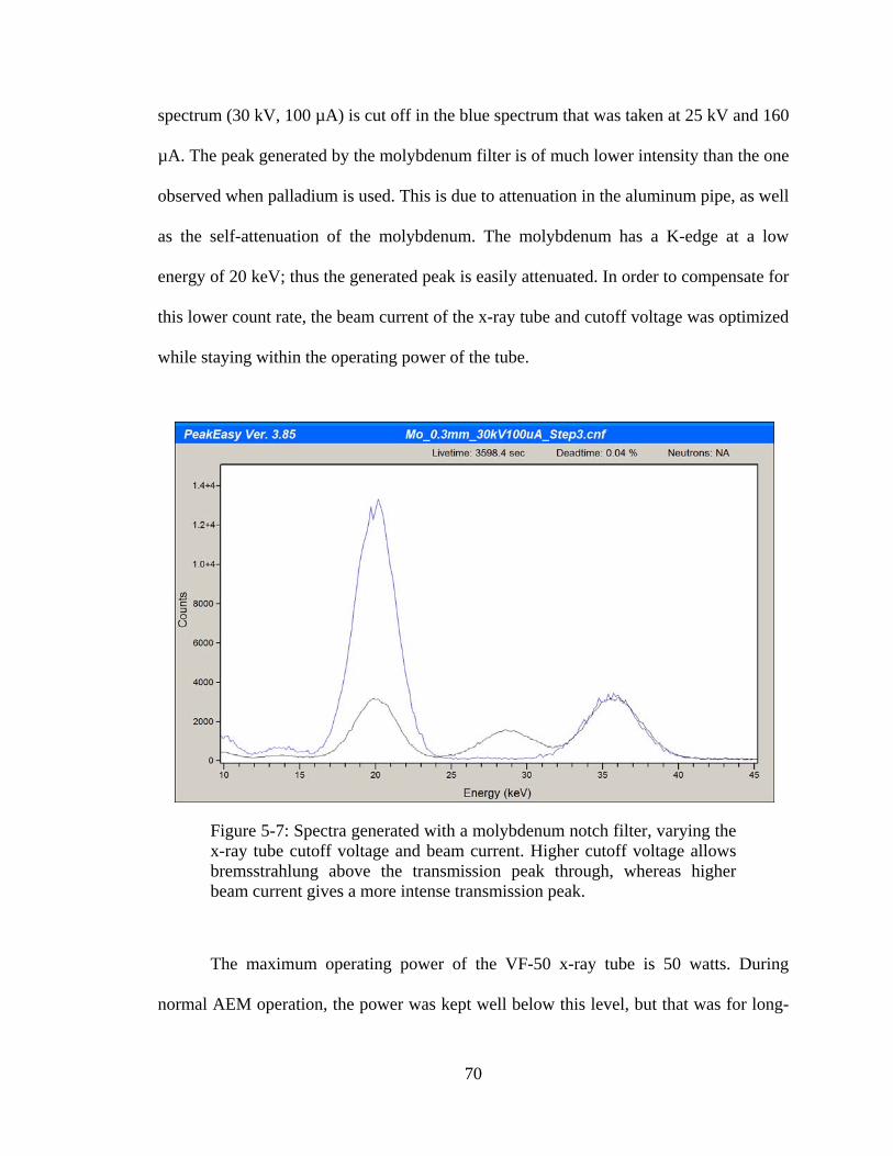
70
spectrum (30 kV, 100 µA) is cut off in the blue spectrum that was taken at 25 kV and 160
µA. The peak generated by the molybdenum filter is of much lower intensity than the one
observed when palladium is used. This is due to attenuation in the aluminum pipe, as well
as the self-attenuation of the molybdenum. The molybdenum has a K-edge at a low
energy of 20 keV; thus the generated peak is easily attenuated. In order to compensate for
this lower count rate, the beam current of the x-ray tube and cutoff voltage was optimized
while staying within the operating power of the tube.
Figure 5-7: Spectra generated with a molybdenum notch filter, varying the x-ray tube cutoff voltage and beam current. Higher cutoff voltage allows bremsstrahlung above the transmission peak through, whereas higher beam current gives a more intense transmission peak.
The maximum operating power of the VF-50 x-ray tube is 50 watts. During
normal AEM operation, the power was kept well below this level, but that was for long-

71
term measurements. Measurement times for the pipe-wall thickness experiment are either
30 or 60 minutes, depending on the count rate in the transmission peak. The final x-ray
tube settings selected for the measurements were 30 kV and 160 µA. Thus the
molybdenum peak was measurable (good enough statistics to analyze with a 3,600-s
count time) in most cases, and the palladium peak still had a reasonable dead time—less
than a 3% maximum—which the LaBr3 detector and Lynx system are easily able to
handle.
A few selected spectra are shown below. First, in Figs. 5.8 and 5.9, spectra taken
with a 0.3-mm-thick palladium notch filter are compared. In those figures, the black line
was taken with 40 Torr of UF6 gas in the pipe, and the blue was an empty pipe
measurement. Figure 5.8 has ROIs highlighted in red, showing the transmission peak at
24.3 keV and the 185.7-keV 235U peak. A log scale was used to make all peaks visible.
Figure 5.9 is a close-up of the transmission peak generated with the palladium notch
filter, showing the effect of attenuation by 40 Torr of UF6. A linear scale was used to
show the difference in spectra.
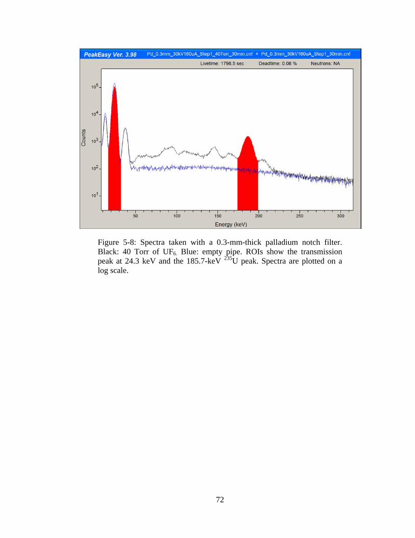
72
Figure 5-8: Spectra taken with a 0.3-mm-thick palladium notch filter. Black: 40 Torr of UF6. Blue: empty pipe. ROIs show the transmission peak at 24.3 keV and the 185.7-keV 235U peak. Spectra are plotted on a log scale.

73
Figure 5-9: Close-up of the palladium transmission peak. Black: transmission through 40 Torr of UF6. Blue: transmission through the empty pipe. Data are displayed on a linear scale to emphasize the difference in peak areas.
Figure 5.10 shows a spectrum taken using a 0.3-mm molybdenum notch filter
with 40 Torr of UF6 in the pipe. ROIs (in red) show the molybdenum transmission peak
at 20 keV and the 185.7-keV 235U peak. In this spectrum there is bremsstrahlung visible
between the molybdenum peak and the 138La x-ray peak. This is because a 30-kV cutoff
voltage on the x-ray tube is used.
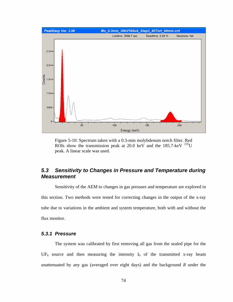
74
Figure 5-10: Spectrum taken with a 0.3-mm molybdenum notch filter. Red ROIs show the transmission peak at 20.0 keV and the 185.7-keV 235U peak. A linear scale was used.
5.3 Sensitivity to Changes in Pressure and Temperature during Measurement
Sensitivity of the AEM to changes in gas pressure and temperature are explored in
this section. Two methods were tested for correcting changes in the output of the x-ray
tube due to variations in the ambient and system temperature, both with and without the
flux monitor.
5.3.1 Pressure
The system was calibrated by first removing all gas from the sealed pipe for the
UF6 source and then measuring the intensity I0 of the transmitted x-ray beam
unattenuated by any gas (averaged over eight days) and the background B under the
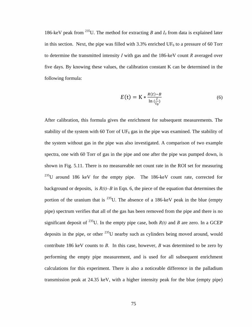
75
186-keV peak from 235U. The method for extracting B and I0 from data is explained later
in this section. Next, the pipe was filled with 3.3% enriched UF6 to a pressure of 60 Torr
to determine the transmitted intensity I with gas and the 186-keV count R averaged over
five days. By knowing these values, the calibration constant K can be determined in the
following formula:
t K ∗
(6)
After calibration, this formula gives the enrichment for subsequent measurements. The
stability of the system with 60 Torr of UF6 gas in the pipe was examined. The stability of
the system without gas in the pipe was also investigated. A comparison of two example
spectra, one with 60 Torr of gas in the pipe and one after the pipe was pumped down, is
shown in Fig. 5.11. There is no measureable net count rate in the ROI set for measuring
235U around 186 keV for the empty pipe. The 186-keV count rate, corrected for
background or deposits, is R(t)–B in Eqn. 6, the piece of the equation that determines the
portion of the uranium that is 235U. The absence of a 186-keV peak in the blue (empty
pipe) spectrum verifies that all of the gas has been removed from the pipe and there is no
significant deposit of 235U. In the empty pipe case, both R(t) and B are zero. In a GCEP
deposits in the pipe, or other 235U nearby such as cylinders being moved around, would
contribute 186 keV counts to B. In this case, however, B was determined to be zero by
performing the empty pipe measurement, and is used for all subsequent enrichment
calculations for this experiment. There is also a noticeable difference in the palladium
transmission peak at 24.35 keV, with a higher intensity peak for the blue (empty pipe)
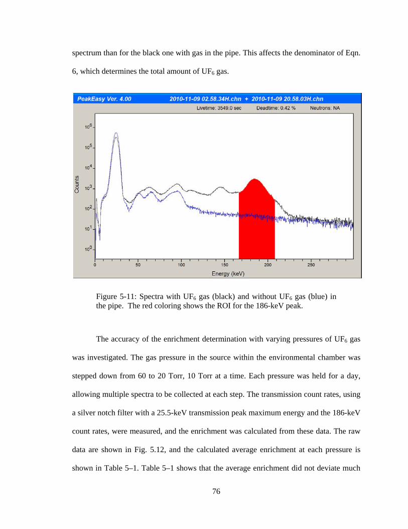
76
spectrum than for the black one with gas in the pipe. This affects the denominator of Eqn.
6, which determines the total amount of UF6 gas.
Figure 5-11: Spectra with UF6 gas (black) and without UF6 gas (blue) in the pipe. The red coloring shows the ROI for the 186-keV peak.
The accuracy of the enrichment determination with varying pressures of UF6 gas
was investigated. The gas pressure in the source within the environmental chamber was
stepped down from 60 to 20 Torr, 10 Torr at a time. Each pressure was held for a day,
allowing multiple spectra to be collected at each step. The transmission count rates, using
a silver notch filter with a 25.5-keV transmission peak maximum energy and the 186-keV
count rates, were measured, and the enrichment was calculated from these data. The raw
data are shown in Fig. 5.12, and the calculated average enrichment at each pressure is
shown in Table 5–1. Table 5–1 shows that the average enrichment did not deviate much
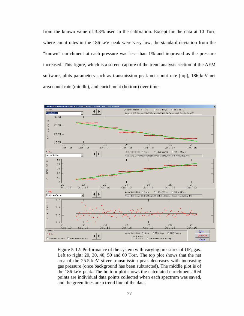
77
from the known value of 3.3% used in the calibration. Except for the data at 10 Torr,
where count rates in the 186-keV peak were very low, the standard deviation from the
“known” enrichment at each pressure was less than 1% and improved as the pressure
increased. This figure, which is a screen capture of the trend analysis section of the AEM
software, plots parameters such as transmission peak net count rate (top), 186-keV net
area count rate (middle), and enrichment (bottom) over time.
Figure 5-12: Performance of the system with varying pressures of UF6 gas. Left to right: 20, 30, 40, 50 and 60 Torr. The top plot shows that the net area of the 25.5-keV silver transmission peak decreases with increasing gas pressure (once background has been subtracted). The middle plot is of the 186-keV peak. The bottom plot shows the calculated enrichment. Red points are individual data points collected when each spectrum was saved, and the green lines are a trend line of the data.
78
The trend analysis portion of the AEM software (from which the screen shot
above was taken) allows user-chosen parameters to be displayed over time. In this case,
the parameter that was changed over time was the pressure, raised in steps from 20 to 60
Torr, 10 Torr at a time. The top plot shows that the net area of the transmission peak
decreases with increasing gas pressure (once background has been subtracted). In the plot
beneath it, the 186-keV peak increases as the gas pressure is raised. The bottom plot
shows that the calculated enrichment holds steady over all of the changes in the gas
pressure. The enrichment plot also shows that the statistics of the enrichment
measurement improve with increasing gas pressure. This improvement is due to the lower
count rates in the 186-keV peak at low pressures.
Table 5-1: Average Enrichments at Various Pressures and the Effect of Count Rates in the 186-keV Peak Shown by the Standard Deviations
A significant effect occurred when the gas was removed from the pipe after it had
been in the pipe for several weeks. As shown in Fig. 5.13, the total count rate in the
spectrum continued to decrease after the gas had been removed. Investigation identified
the cause as the decay of 234Th (half-life 24 days), which is formed by the decay of 238U
Pressure (Torr)
Average Enrichment (%)
Standard Deviation
10 3.279 ± 0.097 2.95%
20 3.319 ± 0.029 0.86%
30 3.329 ± 0.027 0.80%
40 3.324 ± 0.023 0.69%
50 3.318 ± 0.020 0.60%
60 3.322 ± 0.018 0.55%
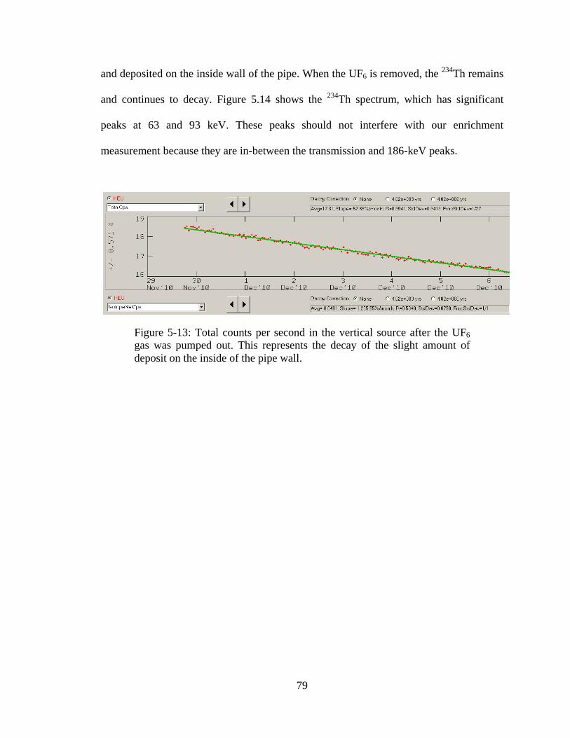
79
and deposited on the inside wall of the pipe. When the UF6 is removed, the 234Th remains
and continues to decay. Figure 5.14 shows the 234Th spectrum, which has significant
peaks at 63 and 93 keV. These peaks should not interfere with our enrichment
measurement because they are in-between the transmission and 186-keV peaks.
Figure 5-13: Total counts per second in the vertical source after the UF6 gas was pumped out. This represents the decay of the slight amount of deposit on the inside of the pipe wall.
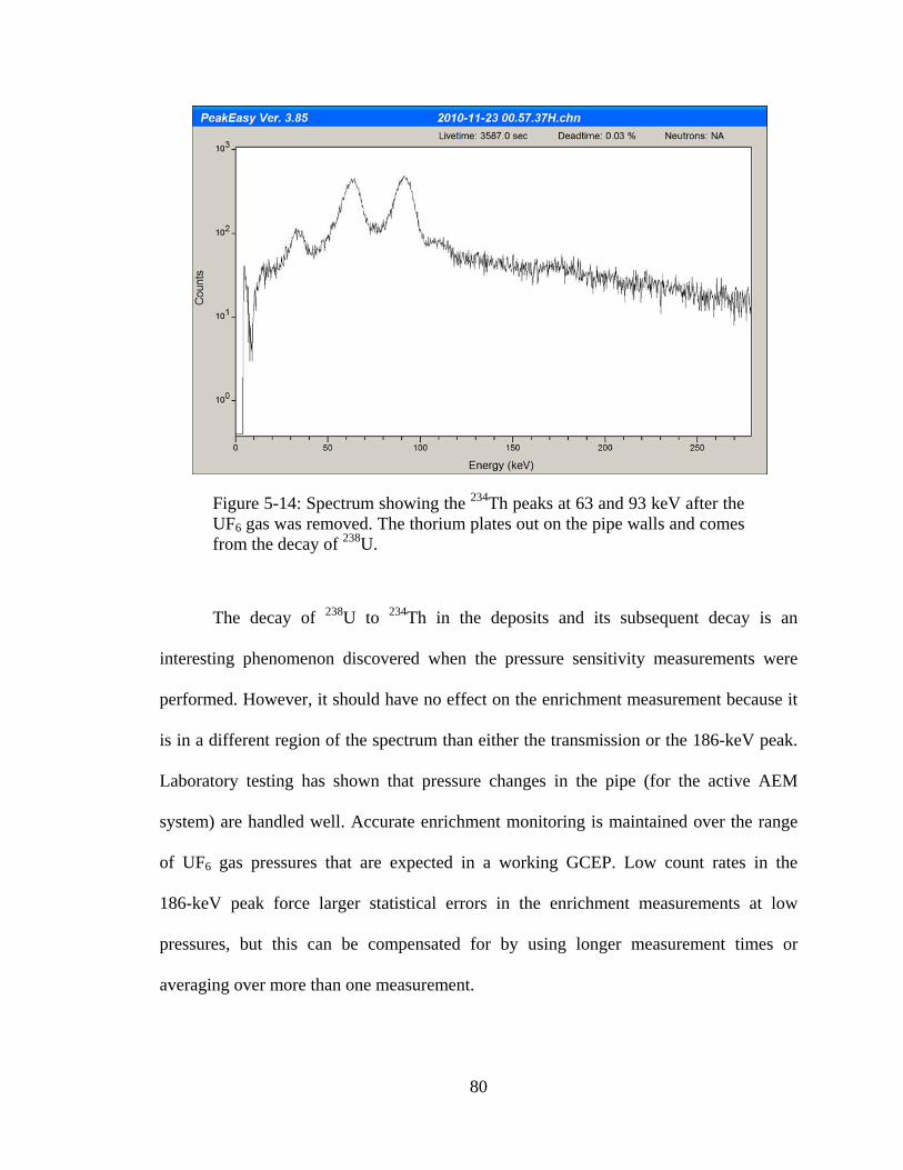
80
Figure 5-14: Spectrum showing the 234Th peaks at 63 and 93 keV after the UF6 gas was removed. The thorium plates out on the pipe walls and comes from the decay of 238U.
The decay of 238U to 234Th in the deposits and its subsequent decay is an
interesting phenomenon discovered when the pressure sensitivity measurements were
performed. However, it should have no effect on the enrichment measurement because it
is in a different region of the spectrum than either the transmission or the 186-keV peak.
Laboratory testing has shown that pressure changes in the pipe (for the active AEM
system) are handled well. Accurate enrichment monitoring is maintained over the range
of UF6 gas pressures that are expected in a working GCEP. Low count rates in the
186-keV peak force larger statistical errors in the enrichment measurements at low
pressures, but this can be compensated for by using longer measurement times or
averaging over more than one measurement.
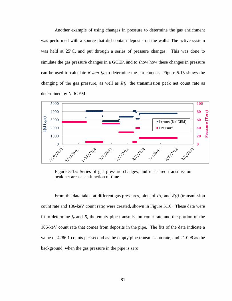
81
Another example of using changes in pressure to determine the gas enrichment
was performed with a source that did contain deposits on the walls. The active system
was held at 25°C, and put through a series of pressure changes. This was done to
simulate the gas pressure changes in a GCEP, and to show how these changes in pressure
can be used to calculate B and I0, to determine the enrichment. Figure 5.15 shows the
changing of the gas pressure, as well as I(t), the transmission peak net count rate as
determined by NaIGEM.
Figure 5-15: Series of gas pressure changes, and measured transmission peak net areas as a function of time.
From the data taken at different gas pressures, plots of I(t) and R(t) (transmission
count rate and 186-keV count rate) were created, shown in Figure 5.16. These data were
fit to determine I0 and B, the empty pipe transmission count rate and the portion of the
186-keV count rate that comes from deposits in the pipe. The fits of the data indicate a
value of 4286.1 counts per second as the empty pipe transmission rate, and 21.008 as the
background, when the gas pressure in the pipe is zero.
0
20
40
60
80
100
0
1000
2000
3000
4000
5000
Pressure(Torr)
I(t)(cps)
Itrans(NaIGEM)
Pressure
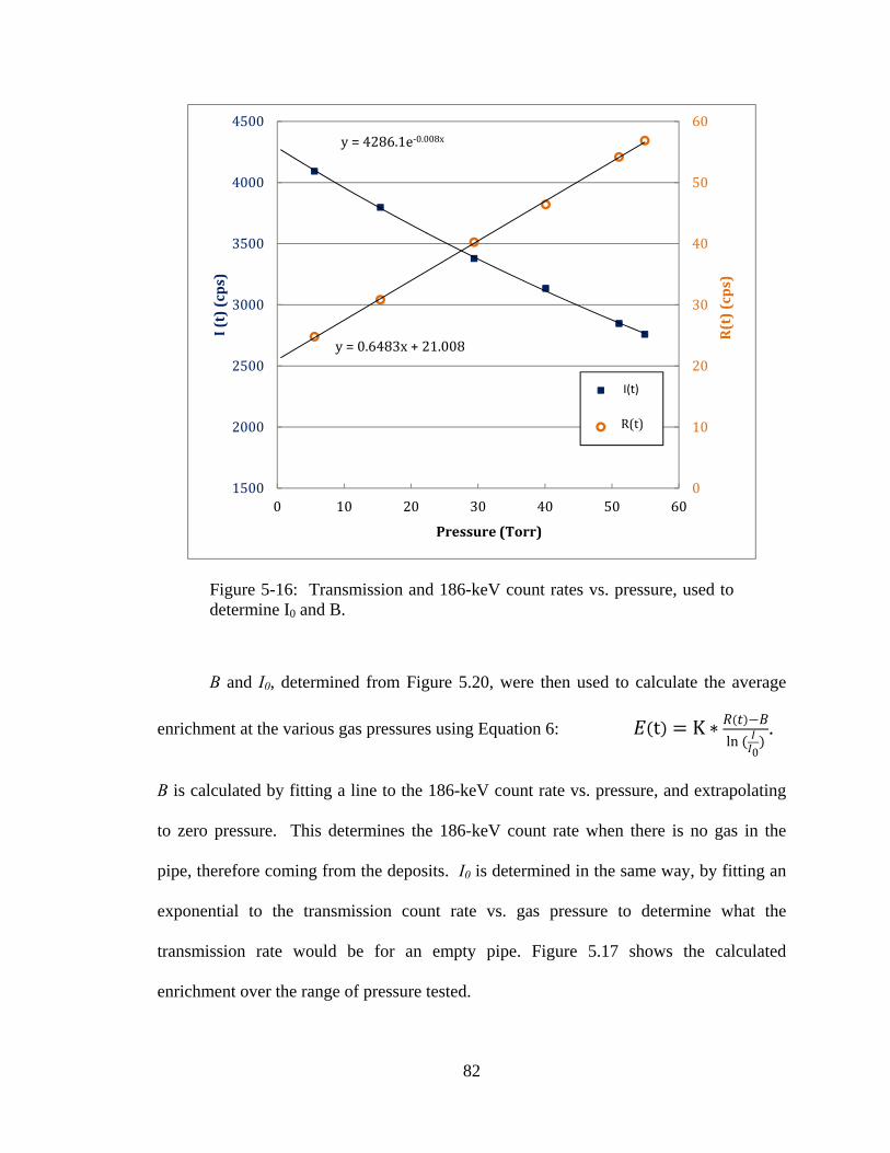
82
Figure 5-16: Transmission and 186-keV count rates vs. pressure, used to determine I0 and B.
B and I0, determined from Figure 5.20, were then used to calculate the average
enrichment at the various gas pressures using Equation 6: t K ∗ln
0
.
B is calculated by fitting a line to the 186-keV count rate vs. pressure, and extrapolating
to zero pressure. This determines the 186-keV count rate when there is no gas in the
pipe, therefore coming from the deposits. I0 is determined in the same way, by fitting an
exponential to the transmission count rate vs. gas pressure to determine what the
transmission rate would be for an empty pipe. Figure 5.17 shows the calculated
enrichment over the range of pressure tested.
y=4286.1e‐0.008x
y=0.6483x+21.008
0
10
20
30
40
50
60
1500
2000
2500
3000
3500
4000
4500
0 10 20 30 40 50 60
R(t)(cps)
I(t)(cps)
Pressure(Torr)
ITrans
I186R(t)
I(t)
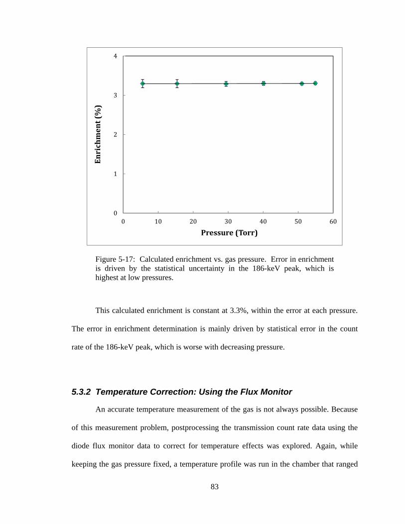
83
Figure 5-17: Calculated enrichment vs. gas pressure. Error in enrichment is driven by the statistical uncertainty in the 186-keV peak, which is highest at low pressures.
This calculated enrichment is constant at 3.3%, within the error at each pressure.
The error in enrichment determination is mainly driven by statistical error in the count
rate of the 186-keV peak, which is worse with decreasing pressure.
5.3.2 Temperature Correction: Using the Flux Monitor
An accurate temperature measurement of the gas is not always possible. Because
of this measurement problem, postprocessing the transmission count rate data using the
diode flux monitor data to correct for temperature effects was explored. Again, while
keeping the gas pressure fixed, a temperature profile was run in the chamber that ranged
0
1
2
3
4
0 10 20 30 40 50 60
Enrichment(%)
Pressure(Torr)
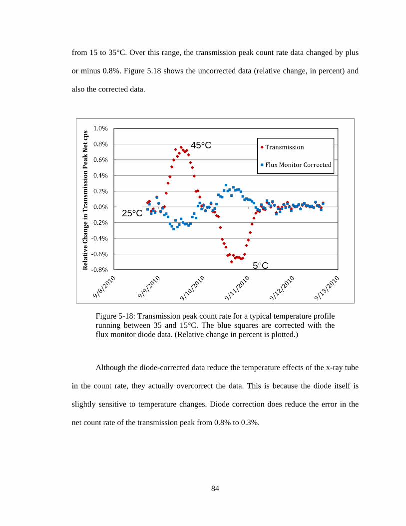
84
from 15 to 35°C. Over this range, the transmission peak count rate data changed by plus
or minus 0.8%. Figure 5.18 shows the uncorrected data (relative change, in percent) and
also the corrected data.
Figure 5-18: Transmission peak count rate for a typical temperature profile running between 35 and 15°C. The blue squares are corrected with the flux monitor diode data. (Relative change in percent is plotted.)
Although the diode-corrected data reduce the temperature effects of the x-ray tube
in the count rate, they actually overcorrect the data. This is because the diode itself is
slightly sensitive to temperature changes. Diode correction does reduce the error in the
net count rate of the transmission peak from 0.8% to 0.3%.
‐0.8%
‐0.6%
‐0.4%
‐0.2%
0.0%
0.2%
0.4%
0.6%
0.8%
1.0%
RelativeChangeinTransm
issionPeakNetcps
Transmission
FluxMonitorCorrected
5°C
25°C
45°C
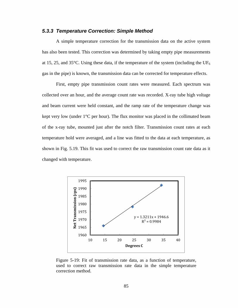
85
5.3.3 Temperature Correction: Simple Method
A simple temperature correction for the transmission data on the active system
has also been tested. This correction was determined by taking empty pipe measurements
at 15, 25, and 35°C. Using these data, if the temperature of the system (including the UF6
gas in the pipe) is known, the transmission data can be corrected for temperature effects.
First, empty pipe transmission count rates were measured. Each spectrum was
collected over an hour, and the average count rate was recorded. X-ray tube high voltage
and beam current were held constant, and the ramp rate of the temperature change was
kept very low (under 1°C per hour). The flux monitor was placed in the collimated beam
of the x-ray tube, mounted just after the notch filter. Transmission count rates at each
temperature hold were averaged, and a line was fitted to the data at each temperature, as
shown in Fig. 5.19. This fit was used to correct the raw transmission count rate data as it
changed with temperature.
Figure 5-19: Fit of transmission rate data, as a function of temperature, used to correct raw transmission rate data in the simple temperature correction method.
y=1.3211x+1946.6R²=0.9984
1960
1965
1970
1975
1980
1985
1990
1995
10 15 20 25 30 35 40
NetTransm
ission(cps)
DegreesC
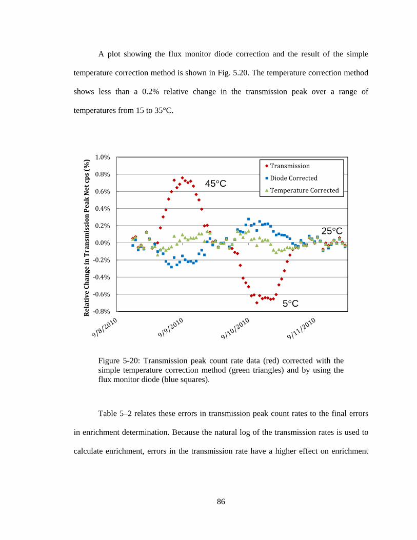
86
A plot showing the flux monitor diode correction and the result of the simple
temperature correction method is shown in Fig. 5.20. The temperature correction method
shows less than a 0.2% relative change in the transmission peak over a range of
temperatures from 15 to 35°C.
Figure 5-20: Transmission peak count rate data (red) corrected with the simple temperature correction method (green triangles) and by using the flux monitor diode (blue squares).
Table 5–2 relates these errors in transmission peak count rates to the final errors
in enrichment determination. Because the natural log of the transmission rates is used to
calculate enrichment, errors in the transmission rate have a higher effect on enrichment
‐0.8%
‐0.6%
‐0.4%
‐0.2%
0.0%
0.2%
0.4%
0.6%
0.8%
1.0%
RelativeChangeinTransm
issionPeakNetcps(%
)
Transmission
DiodeCorrected
TemperatureCorrected
5°C
45°C
25°C
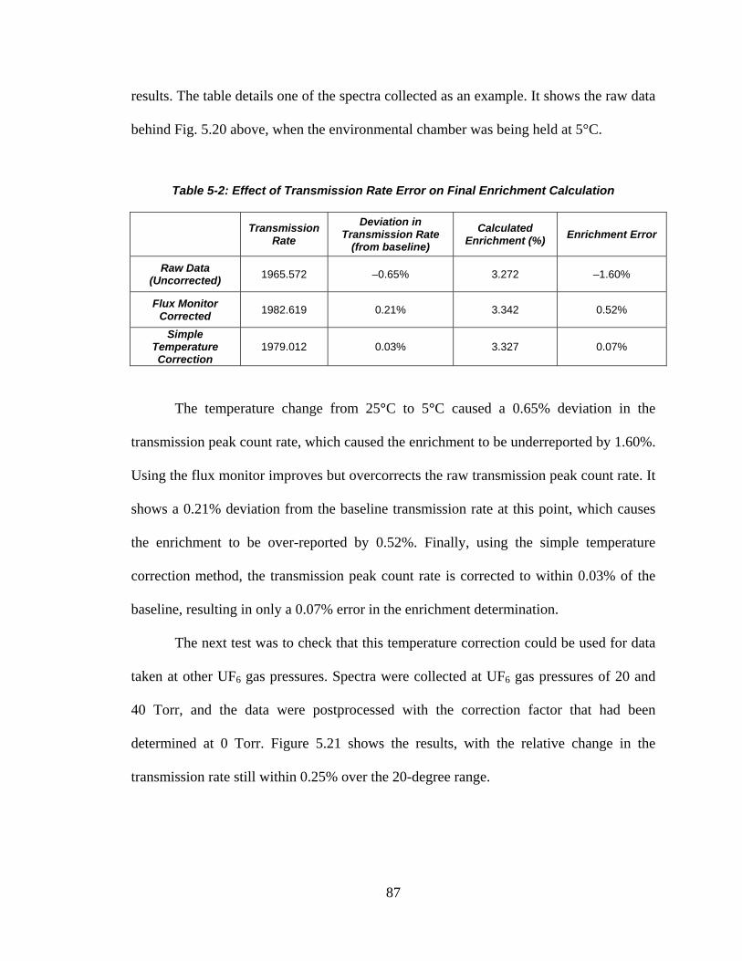
87
results. The table details one of the spectra collected as an example. It shows the raw data
behind Fig. 5.20 above, when the environmental chamber was being held at 5°C.
Table 5-2: Effect of Transmission Rate Error on Final Enrichment Calculation
Transmission
Rate
Deviation in Transmission Rate
(from baseline)
Calculated Enrichment (%)
Enrichment Error
Raw Data (Uncorrected)
1965.572 –0.65% 3.272 –1.60%
Flux Monitor Corrected
1982.619 0.21% 3.342 0.52%
Simple Temperature Correction
1979.012 0.03% 3.327 0.07%
The temperature change from 25°C to 5°C caused a 0.65% deviation in the
transmission peak count rate, which caused the enrichment to be underreported by 1.60%.
Using the flux monitor improves but overcorrects the raw transmission peak count rate. It
shows a 0.21% deviation from the baseline transmission rate at this point, which causes
the enrichment to be over-reported by 0.52%. Finally, using the simple temperature
correction method, the transmission peak count rate is corrected to within 0.03% of the
baseline, resulting in only a 0.07% error in the enrichment determination.
The next test was to check that this temperature correction could be used for data
taken at other UF6 gas pressures. Spectra were collected at UF6 gas pressures of 20 and
40 Torr, and the data were postprocessed with the correction factor that had been
determined at 0 Torr. Figure 5.21 shows the results, with the relative change in the
transmission rate still within 0.25% over the 20-degree range.
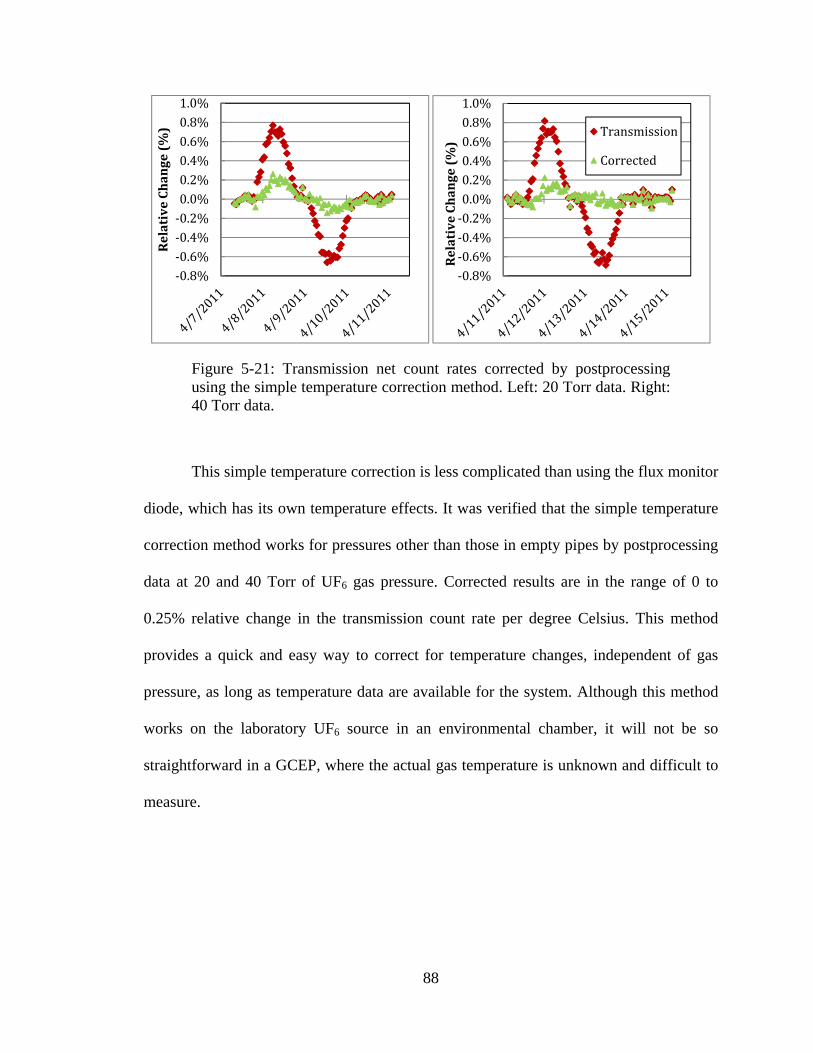
88
Figure 5-21: Transmission net count rates corrected by postprocessing using the simple temperature correction method. Left: 20 Torr data. Right: 40 Torr data.
This simple temperature correction is less complicated than using the flux monitor
diode, which has its own temperature effects. It was verified that the simple temperature
correction method works for pressures other than those in empty pipes by postprocessing
data at 20 and 40 Torr of UF6 gas pressure. Corrected results are in the range of 0 to
0.25% relative change in the transmission count rate per degree Celsius. This method
provides a quick and easy way to correct for temperature changes, independent of gas
pressure, as long as temperature data are available for the system. Although this method
works on the laboratory UF6 source in an environmental chamber, it will not be so
straightforward in a GCEP, where the actual gas temperature is unknown and difficult to
measure.
‐0.8%‐0.6%‐0.4%‐0.2%0.0%0.2%0.4%0.6%0.8%1.0%
RelativeChange(%)
‐0.8%‐0.6%‐0.4%‐0.2%0.0%0.2%0.4%0.6%0.8%1.0%
RelativeChange(%)
Transmission
Corrected
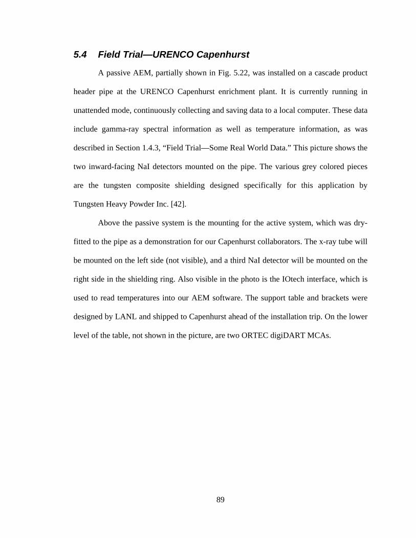
89
5.4 Field Trial—URENCO Capenhurst
A passive AEM, partially shown in Fig. 5.22, was installed on a cascade product
header pipe at the URENCO Capenhurst enrichment plant. It is currently running in
unattended mode, continuously collecting and saving data to a local computer. These data
include gamma-ray spectral information as well as temperature information, as was
described in Section 1.4.3, “Field Trial—Some Real World Data.” This picture shows the
two inward-facing NaI detectors mounted on the pipe. The various grey colored pieces
are the tungsten composite shielding designed specifically for this application by
Tungsten Heavy Powder Inc. [42].
Above the passive system is the mounting for the active system, which was dry-
fitted to the pipe as a demonstration for our Capenhurst collaborators. The x-ray tube will
be mounted on the left side (not visible), and a third NaI detector will be mounted on the
right side in the shielding ring. Also visible in the photo is the IOtech interface, which is
used to read temperatures into our AEM software. The support table and brackets were
designed by LANL and shipped to Capenhurst ahead of the installation trip. On the lower
level of the table, not shown in the picture, are two ORTEC digiDART MCAs.
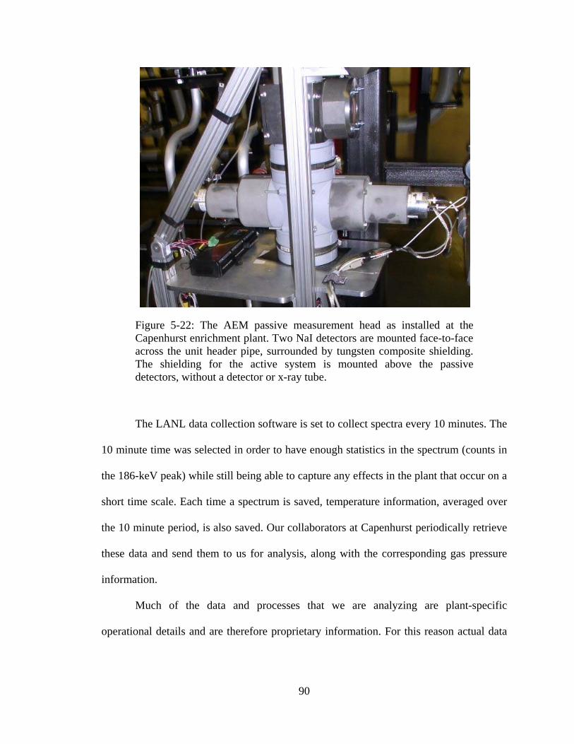
90
Figure 5-22: The AEM passive measurement head as installed at the Capenhurst enrichment plant. Two NaI detectors are mounted face-to-face across the unit header pipe, surrounded by tungsten composite shielding. The shielding for the active system is mounted above the passive detectors, without a detector or x-ray tube.
The LANL data collection software is set to collect spectra every 10 minutes. The
10 minute time was selected in order to have enough statistics in the spectrum (counts in
the 186-keV peak) while still being able to capture any effects in the plant that occur on a
short time scale. Each time a spectrum is saved, temperature information, averaged over
the 10 minute period, is also saved. Our collaborators at Capenhurst periodically retrieve
these data and send them to us for analysis, along with the corresponding gas pressure
information.
Much of the data and processes that we are analyzing are plant-specific
operational details and are therefore proprietary information. For this reason actual data
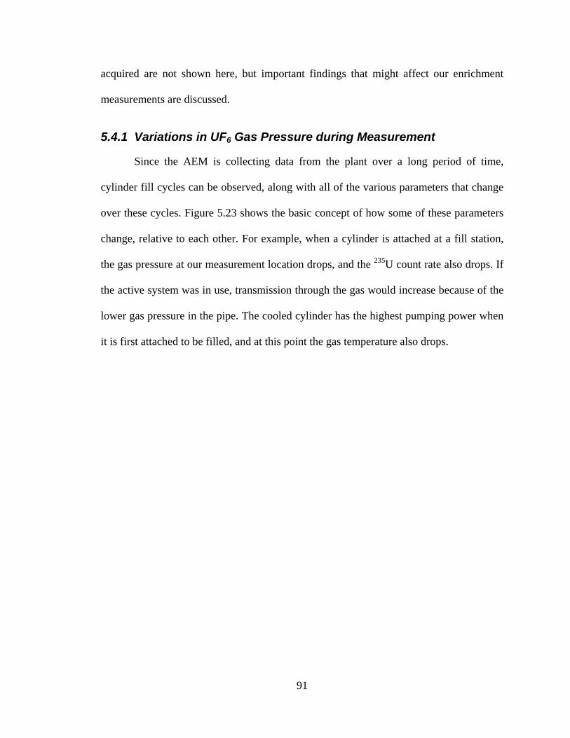
91
acquired are not shown here, but important findings that might affect our enrichment
measurements are discussed.
5.4.1 Variations in UF6 Gas Pressure during Measurement
Since the AEM is collecting data from the plant over a long period of time,
cylinder fill cycles can be observed, along with all of the various parameters that change
over these cycles. Figure 5.23 shows the basic concept of how some of these parameters
change, relative to each other. For example, when a cylinder is attached at a fill station,
the gas pressure at our measurement location drops, and the 235U count rate also drops. If
the active system was in use, transmission through the gas would increase because of the
lower gas pressure in the pipe. The cooled cylinder has the highest pumping power when
it is first attached to be filled, and at this point the gas temperature also drops.
92
Figure 5-23: Schematic of measurement conditions in the unit header pipe during normal plant operation. When a new cylinder is connected to be filled, the gas pressure drops, the gas temperature and the 235U count rate drop, and transmission through the gas increases. The dashed lines represent B, the contribution to the 235U count rate from background (and deposits), and I0, the empty pipe transmission scenario.
The idea of using pressure transients, or rapid drops in the UF6 gas pressure in the
pipe at the measurement location when a new fill cylinder is attached, was first presented
at the European Safeguards Research and Development Association’s 2010 meeting [43].
These rapid pressure changes can be used to calibrate the passive portion of the AEM,
since the enrichment cannot change in such a short time period.
5.4.2 Background Determination (Including Pipe Deposits)
By measuring the 186-keV count rate before and after a pressure transient, we can
determine B, the background (which includes deposits) in Eqn. 7.
t K ∗ R t B (7)
93
This is similar to the transmission-based enrichment formula given in Eqn. 5, but
instead of using an attenuation term in the denominator to determine the total uranium
content, it uses temperature corrected (T(t)) gas pressure (p(t)) to determine the total
amount of gas in the pipe. This calculation is possible because the enrichment in a GCEP
cascade cannot change over such a short period of time and can be treated as a constant
over the pressure transient. Therefore, since the measurement system operates with
declared operator pressure readings, one can interpolate down to a zero pressure and
determine the portion of the 186-keV signal that is coming from background or the
background plus pipe deposits. This is a fairly straightforward calculation, since it is
assumed that the background B is also a constant over the pressure transient time. In the
same way, with the active AEM, we could use this method to solve for I0, the empty pipe
transmission count rate in Eqn. 6 from Chapter 5, “Experimental Measurements.”
Another method that has been even more accurate for determining background is
to plot the calculated enrichment errors over time vs. the pressure at which the spectrum
was collected. Then B can be optimized so that the plot of the enrichment error vs.
pressure has a slope of zero—ensuring that the background determination is independent
of gas pressure and, therefore, as accurate as possible.
5.4.3 Temperature Effects
The greatest challenge for calibrating the passive system, however, is the gas
temperature, which not directly measurable. While there are temperature sensors on the
aluminum pipe, the steel bellows after the compressor (just upstream of the AEM) and
measuring ambient temperature, there is no direct measurement of the gas temperature.
Furthermore, the temperature is the one variable that cannot be treated as a constant

94
during a pressure transient. For analysis of the current data being taken with the AEM in
Capenhurst, a temperature correction factor is used that is derived from a combination of
the measured temperatures. Once the active system is installed next to the passive system,
the transmission measurement results can be used as an additional piece of information to
help correct for gas temperature changes.
95
6 Pipe-wall Thickness Results and Analysis
This chapter presents the results and analysis of the pipe-wall thickness
experiments. First the measured transmission ratios are shown to be independent of gas
pressure, which allows this method to be used for an unknown gas pressure or in a
facility where the AEM operator does not have access to facility pressure declarations.
Next a calibration curve has been created, using a standard pipe of three known
thicknesses as the basis for determining unknown pipe thicknesses. Finally, a brief
discussion is presented, comparing the earlier analytical results to the experimental ones.
6.1 Experimental Results
A series of measurements was taken for the pipe thickness experiment, varying a
number of factors.
1. Two different notch filters were used at each measurement setting:
molybdenum and palladium.
2. Three thicknesses of each filter material were used: 0.3, 0.4, and 0.5 mm.
3. The transmission measurements were performed on three pipe thicknesses, as
shown in Fig. 2.6.
4. The UF6 gas pressure in the pipe was increased in steps up to 50 Torr.
After the data were collected, they were analyzed with a version of Ray
Gunnink’s NaIGEM software [44], which he modified so it could be used to determine
the net areas of both the 186-keV peak from the UF6 and the transmission peak at either
20.0 keV (molybdenum filter) or 24.35 keV (palladium filter). Figure 6.1 shows a screen
shot of a NaIGEM analysis in progress.
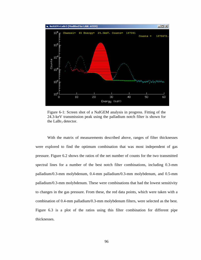
96
Figure 6-1: Screen shot of a NaIGEM analysis in progress. Fitting of the 24.3-keV transmission peak using the palladium notch filter is shown for the LaBr3 detector.
With the matrix of measurements described above, ranges of filter thicknesses
were explored to find the optimum combination that was most independent of gas
pressure. Figure 6.2 shows the ratios of the net number of counts for the two transmitted
spectral lines for a number of the best notch filter combinations, including 0.3-mm
palladium/0.3-mm molybdenum, 0.4-mm palladium/0.3-mm molybdenum, and 0.5-mm
palladium/0.3-mm molybdenum. These were combinations that had the lowest sensitivity
to changes in the gas pressure. From these, the red data points, which were taken with a
combination of 0.4-mm palladium/0.3-mm molybdenum filters, were selected as the best.
Figure 6.3 is a plot of the ratios using this filter combination for different pipe
thicknesses.
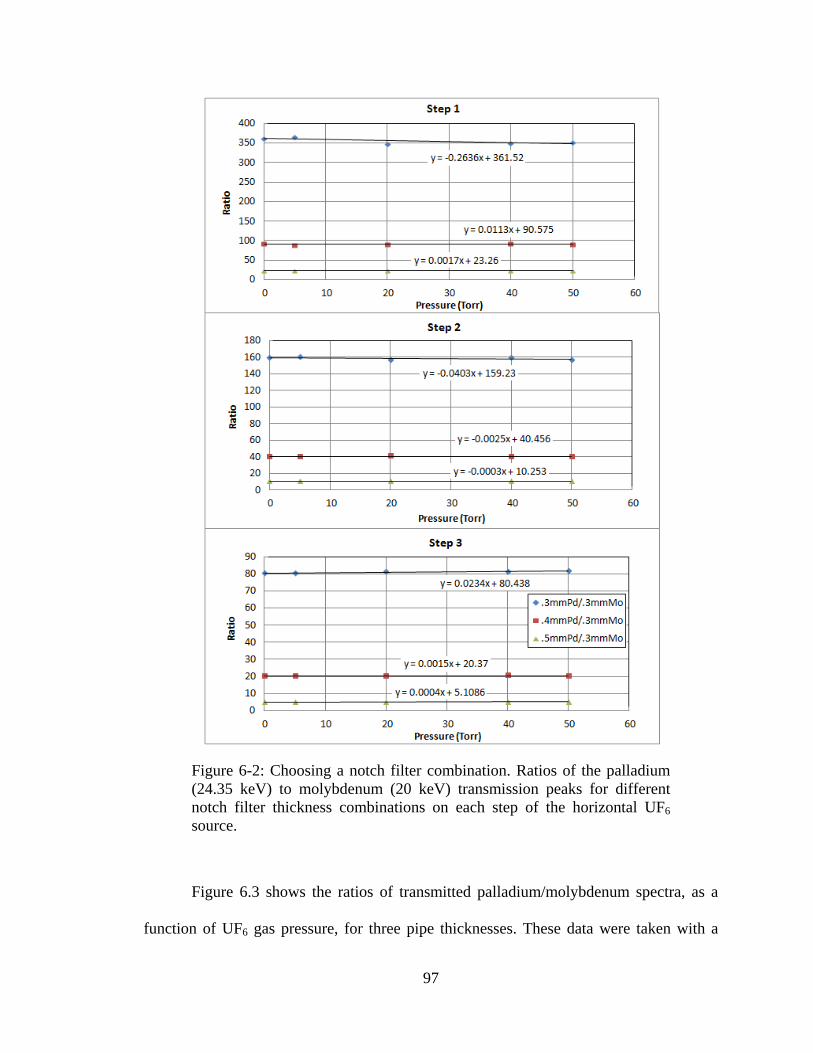
97
Figure 6-2: Choosing a notch filter combination. Ratios of the palladium (24.35 keV) to molybdenum (20 keV) transmission peaks for different notch filter thickness combinations on each step of the horizontal UF6 source.
Figure 6.3 shows the ratios of transmitted palladium/molybdenum spectra, as a
function of UF6 gas pressure, for three pipe thicknesses. These data were taken with a
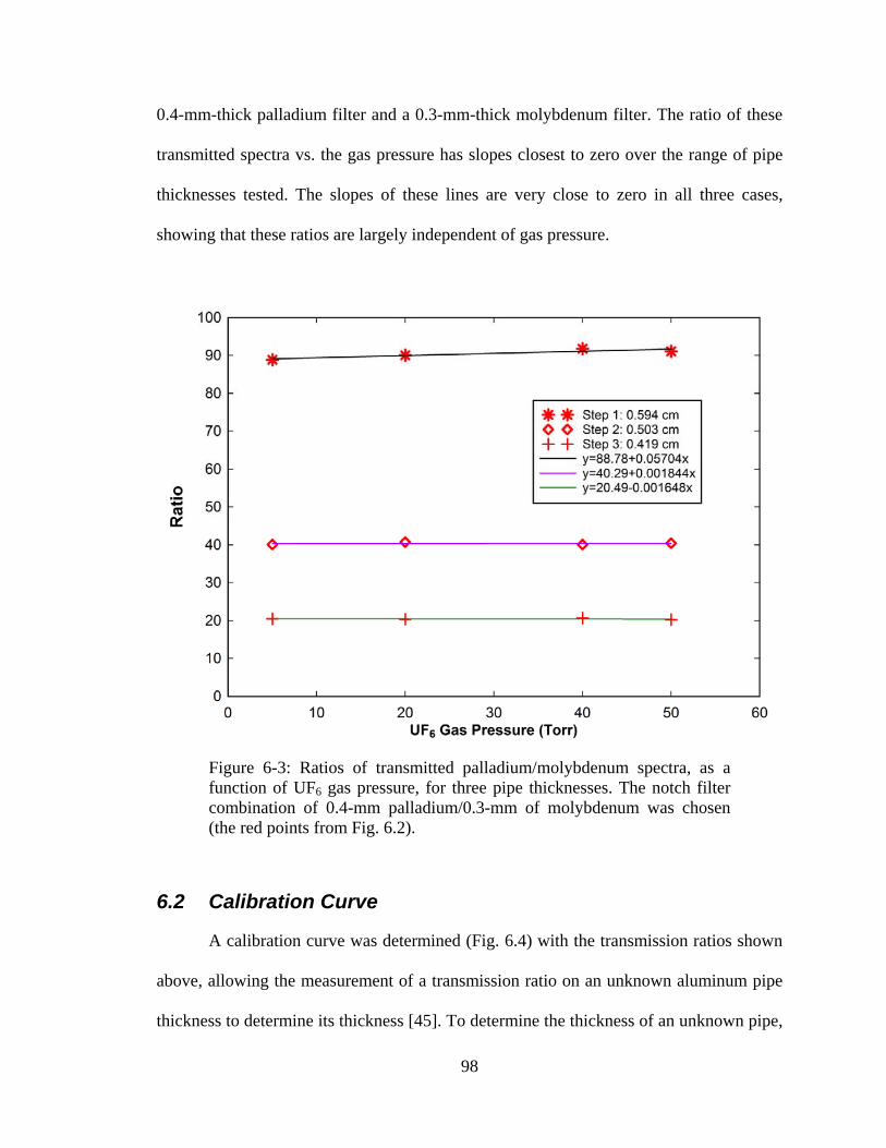
98
0.4-mm-thick palladium filter and a 0.3-mm-thick molybdenum filter. The ratio of these
transmitted spectra vs. the gas pressure has slopes closest to zero over the range of pipe
thicknesses tested. The slopes of these lines are very close to zero in all three cases,
showing that these ratios are largely independent of gas pressure.
Figure 6-3: Ratios of transmitted palladium/molybdenum spectra, as a function of UF6 gas pressure, for three pipe thicknesses. The notch filter combination of 0.4-mm palladium/0.3-mm of molybdenum was chosen (the red points from Fig. 6.2).
6.2 Calibration Curve
A calibration curve was determined (Fig. 6.4) with the transmission ratios shown
above, allowing the measurement of a transmission ratio on an unknown aluminum pipe
thickness to determine its thickness [45]. To determine the thickness of an unknown pipe,
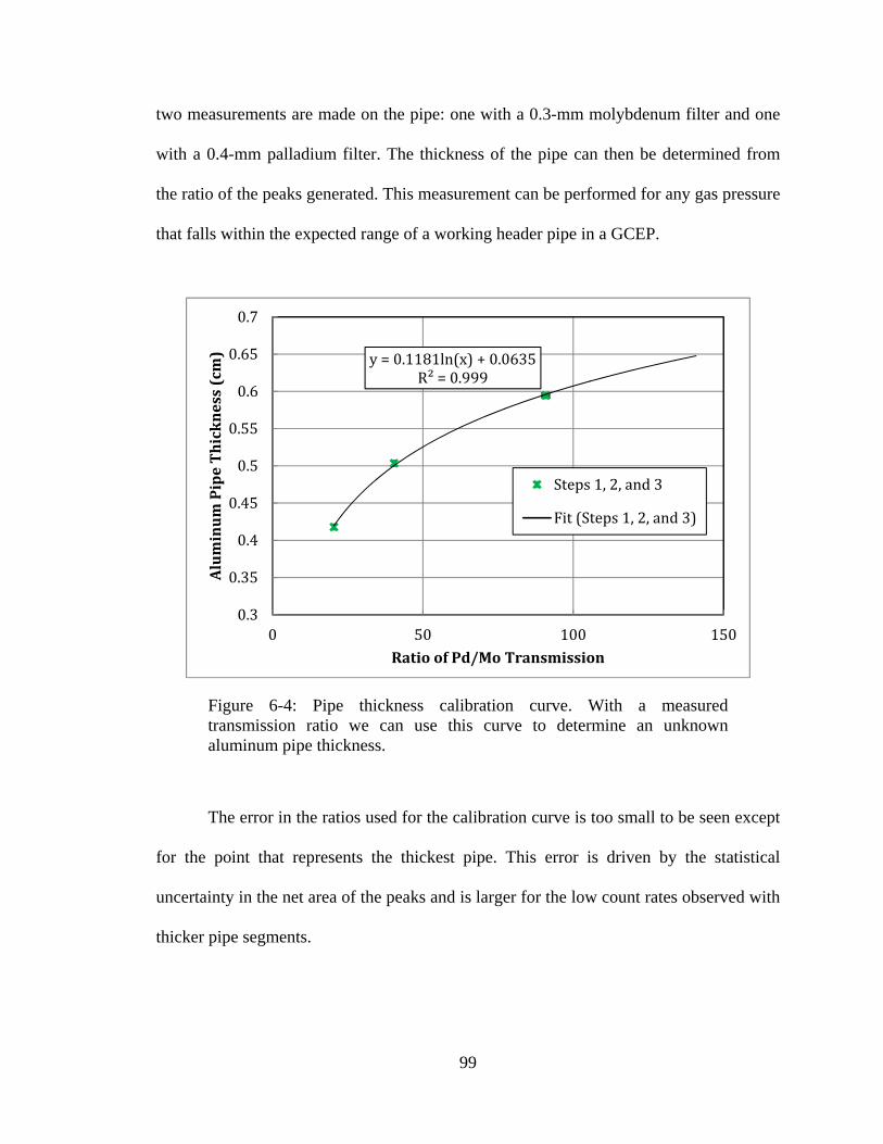
99
two measurements are made on the pipe: one with a 0.3-mm molybdenum filter and one
with a 0.4-mm palladium filter. The thickness of the pipe can then be determined from
the ratio of the peaks generated. This measurement can be performed for any gas pressure
that falls within the expected range of a working header pipe in a GCEP.
Figure 6-4: Pipe thickness calibration curve. With a measured transmission ratio we can use this curve to determine an unknown aluminum pipe thickness.
The error in the ratios used for the calibration curve is too small to be seen except
for the point that represents the thickest pipe. This error is driven by the statistical
uncertainty in the net area of the peaks and is larger for the low count rates observed with
thicker pipe segments.
y=0.1181ln(x)+0.0635R²=0.999
0.3
0.35
0.4
0.45
0.5
0.55
0.6
0.65
0.7
0 50 100 150
AluminumPipeThickness(cm)
RatioofPd/MoTransmission
Steps1,2,and3
Fit(Steps1,2,and3)
100
6.3 “Unknown” Pipe Thickness Measurements
Next the two-step transmission measurement through three “unknown” pipe
thicknesses was performed. Again, standard 6061 aluminum ¼”-thick pipes were used.
Two sections of this pipe were machined down to thicknesses that were within the
expected range of the header pipe thickness in a GCEP. A third pipe section that had a
thickness out of our expected operating range was measured as well. Using the
calibration curve that was achieved with the three-step source, dcalc, the calculated
thickness of each pipe was determined. Once the transmission measurements had been
performed and spectra had been collected, each pipe was cut at the transmission location
for precise thickness measurements. The pipes were measured with a tube micrometer at
two locations—the “entry” and “exit” spots of the beam—and averaged. Figure 6.5
shows the measured thickness of each pipe segment as a function of the ratio for each of
the unknown pipe thicknesses. Error in the measured ratio comes from error in the
calculation of the transmission peak net areas, as determined by the NaIGEM software.
The error bars are too small to see on all but the ratio for the thickest section of pipe. This
error was driven by the statistical uncertainty in the molybdenum transmission peak,
which has the highest attenuation in the pipe.
101
Figure 6-5: Unknown thickness data points plotted against the calibration curve. Most of the error bars are smaller than the data points. True caliper-measured values for the pipe thicknesses were used for plotting the unknown pipes. In thicker pipes, statistics in the transmission peak will drive the error in the thickness determination when using the two-energy method.
Table 6–1 shows the ratio measured for each pipe thickness, the measured and
calculated pipe thicknesses, and the percent difference in calculation using the two-step
method. All three were calculated within 2% accuracy. The thickest pipe segment is out
of the range of pipe thicknesses that we should encounter in a GCEP header pipe. This
method loses accuracy for increasing pipe thicknesses because of the low transmission
count rates seen in the detector in these cases. While the method still works, the error in
the net area of the transmission peak gets too large because of the statistics. This is why
the thickest unknown pipe ratio is the only one with visible error bars. Table 6-1 also
0.3
0.35
0.4
0.45
0.5
0.55
0.6
0.65
0.7
0 50 100 150
AluminumPipeThickness(cm)
RatioofPd/MoTransmission
Steps1,2,and3
UnknownPipeThicknesses

102
shows the effect of the pipe thickness error when determining the relative enrichment
error, and the error in a 5% enriched gas, as an example.
Table 6-1: Pipe Thickness Results
Pd/Mo Ratio dmeas (cm) dcalc (cm) Difference
(%) Enrichment
Error Enrichment
(%)
33.933 ± 0.132 0.472 ± 0.0018 0.480 ± 0.0001 1.7 8.3% 5.0±0.4
74.725 ± 0.750 0.561 ± 0.0024 0.573 ± 0.0089 2.0 11.6% 5.0±0.6
131.315 ± 2.843 0.632 ± 0.0016 0.640 ± 0.0073 1.2 7.8% 5.0±0.4
There appears to be a systematic error to the data, since all of our measurements
fall below the calibration curve. This may be because unknown pipes, while being of the
same alloy as the one used to create the calibration curve, may have had slightly different
amounts of components such as copper, magnesium, silicon, etc. This may introduce a
small error when performing real measurements in an enrichment plant, as will be
determined by the results of the Capenhurst active AEM installation trip. However, there
are only small variations in alloy materials allowed in these aluminum pipes, as shown in
Table 6–2.
6.4 Comparison between Analytical/Experimental Results
In all of the analytical calculations performed, aluminum was used for the pipe
material in a slab geometry. This was an approximation—the actual measurements were
done with an aluminum alloy in a pipe geometry. The pipe used for the three-step source
was a 6061 alloy with a nominal composition of 0.15% copper, 0.8% magnesium, and
0.4% silicon, with the remainder being aluminum [46]. This could be one reason why the
103
analytical notch filter thickness determination was slightly off but still close enough to
give a good range of thicknesses of molybdenum and palladium to test. Table 6–2 shows
the alloy composition of 6061 aluminum, detailing the ranges of materials that are
accepted [47].
Table 6-2: 6061 Aluminum Alloy Composition
Material Amount (%)
Aluminum Balance
Chromium 0.04–0.35
Copper 0.15–0.4
Iron 0–0.7
Magnesium 0.8–1.2
Manganese 0.15 max
Other (Each)
0.15 max 0.05 max
Silicon 0.4–0.8
Titanium 0.15 max
Zinc 0.25 max
Calculations were performed to compare spectra generated using 0.3-mm
molybdenum and 0.4-m palladium notch filters, for a 1-cm-thick aluminum pipe and a
1-cm-thick aluminum alloy pipe. Assuming a “worst-case scenario,” that the three-step
pipe used to generate the calibration curve was pure aluminum, another curve was fit to
compare it to using the high end of all of the alloy materials. This is shown in Figure 6.6,
along with the calculated ratios for those three pipe thicknesses, using the density and
attenuation coefficients calculated for this aluminum alloy.
104
Figure 6-6: Calculated ratios of the "worst case" aluminum alloy, compared to the three-step pipe and the unknown pipes.
Table 6-3 shows what the calculated thickness error would be when using the
calibration curve generated with the three step source on pipes made of the worst case
6061 aluminum alloy. While the relative enrichment errors are high, the effect on the
final calculated enrichment (shown again here with an example of a 5% enriched gas) are
acceptable. If the goal of this system is to determine whether a product is low or highly
enriched, the method will definitely work.
0.3
0.35
0.4
0.45
0.5
0.55
0.6
0.65
0.7
0 20 40 60 80 100 120 140 160
AluminumPipethickness(cm)
RatioofPd/MoTransmission
Steps1,2,and3
UnknownPipeThicknesses
Calculatedworstcase(alloy)
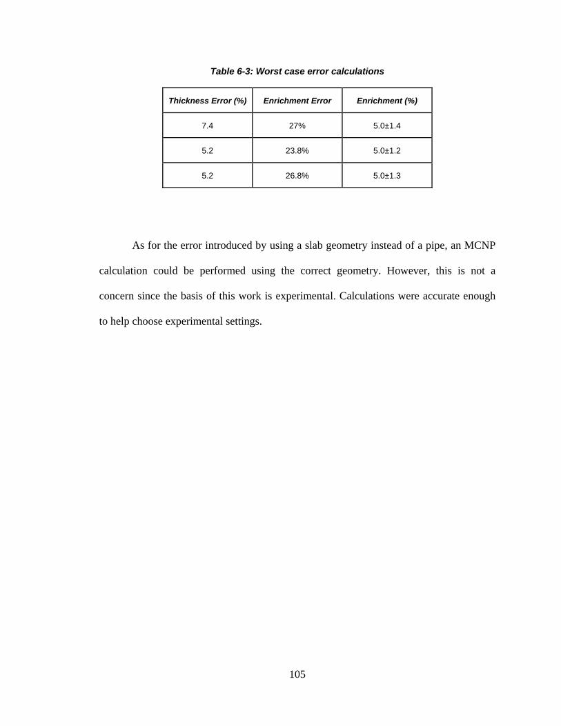
105
Table 6-3: Worst case error calculations
Thickness Error (%) Enrichment Error Enrichment (%)
7.4 27% 5.0±1.4
5.2 23.8% 5.0±1.2
5.2 26.8% 5.0±1.3
As for the error introduced by using a slab geometry instead of a pipe, an MCNP
calculation could be performed using the correct geometry. However, this is not a
concern since the basis of this work is experimental. Calculations were accurate enough
to help choose experimental settings.
106
7 Error Analysis
The following formula, the general formula for error propagation, is used as the
basis of this error analysis section:
q = f(x1,x2,x3,x4) , and (8)
q = . (9)
7.1 Errors in Determining Pipe-wall Thickness
The first section details the calculated errors in the determination of the pipe-wall
thickness. This includes physical measurement errors, errors in the transmission peak net
areas due to statistical uncertainties, and a comparison of the effect of the wall thickness
vs. instrument errors on the final enrichment determination.
7.1.1 “Unknown” Pipe Thicknesses Measurement
After the transmission measurements were completed, the empty pipes of
“unknown thicknesses” were cut so their thicknesses at the measurement location
(directly where the beam passed through) could be measured. Each pipe thickness was
measured in two locations across from each other on the pipe. Ten measurements were
performed in each spot with a pipe micrometer. The standard deviation was calculated at
each location (of 10 measurements), and the average thickness of each pipe section was
calculated.
The average thickness of each pipe section was calculated with the following
equation:
107
, (10)
and the error in the average thickness is
. (11)
In this way, the unknown pipe thicknesses were measured to the values listed as
dmeas in Table 6–1.
7.1.2 Measured Ratios
The errors in the ratios of the transmission peaks using molybdenum and
palladium filters were derived from the reported errors in net peak areas, as determined
by the NaIGEM software. NaIGEM reports an error for each net area that it fits and
calculates. Figure 7.1 shows an example of a NaIGEM fit of the 186-keV region of a
spectrum taken with the LaBr3 detector with 50 Torr of UF6 gas in the horizontal source.
Background is shown by the light blue line, and contributions from other 235U peaks at
144, 163, and 205 keV are taken into account (shown by the green line) when fitting the
186-keV peak.
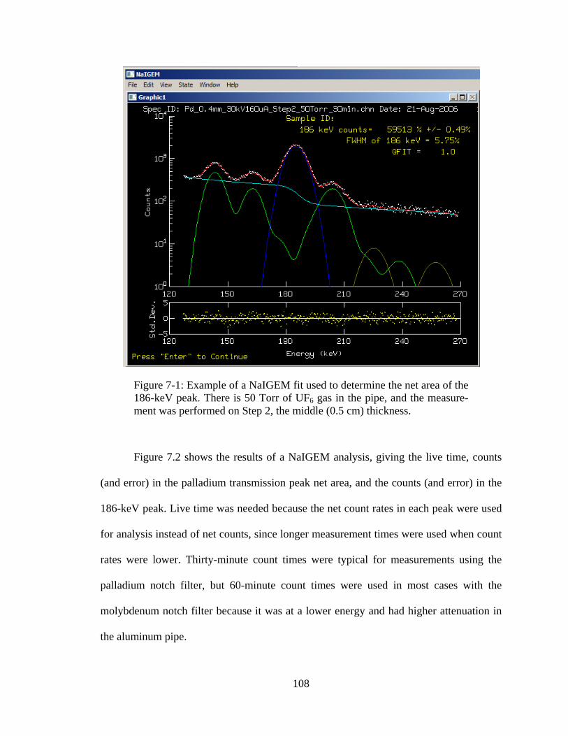
108
Figure 7-1: Example of a NaIGEM fit used to determine the net area of the 186-keV peak. There is 50 Torr of UF6 gas in the pipe, and the measure-ment was performed on Step 2, the middle (0.5 cm) thickness.
Figure 7.2 shows the results of a NaIGEM analysis, giving the live time, counts
(and error) in the palladium transmission peak net area, and the counts (and error) in the
186-keV peak. Live time was needed because the net count rates in each peak were used
for analysis instead of net counts, since longer measurement times were used when count
rates were lower. Thirty-minute count times were typical for measurements using the
palladium notch filter, but 60-minute count times were used in most cases with the
molybdenum notch filter because it was at a lower energy and had higher attenuation in
the aluminum pipe.
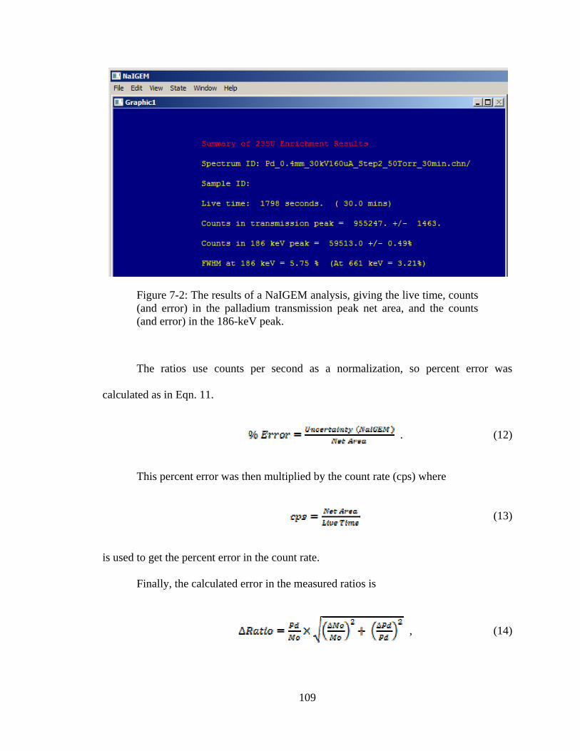
109
Figure 7-2: The results of a NaIGEM analysis, giving the live time, counts (and error) in the palladium transmission peak net area, and the counts (and error) in the 186-keV peak.
The ratios use counts per second as a normalization, so percent error was
calculated as in Eqn. 11.
. (12)
This percent error was then multiplied by the count rate (cps) where
(13)
is used to get the percent error in the count rate.
Finally, the calculated error in the measured ratios is
, (14)
110
where palladium and molybdenum are the net areas of the transmission peaks with each
of the notch filters, and ΔMo and ΔPd are the uncertainties in the net areas of each peak.
This was used to determine the error in the ratios of the unknown pipe thicknesses in
Table 6–1.
7.1.3 “Unknown” Pipe Thicknesses Calculation
To calculate the thicknesses of the unknown pipes, the calibration curve shown in
Fig. 6.4 was used. This curve is a fit to the measured ratios of the palladium to
molybdenum transmission peaks for each pipe segment, with errors described above. The
fit is given by the following equation:
. (15)
To find the error in dcalc, the calculated pipe thicknesses, the above fit for dcalc was
used to determine the error in dcalc for each pipe thickness. Using Eqn. 9, it follows that
q = , (16)
where q = , and x1 = .
Therefore,
= . (17)
Because
, (18)
111
we find that
= , (19)
which because we already solved for ΔRatio above, simplifies to
. (20)
7.2 Enrichment Error from Wall Thickness Measurement Error
The following error analysis examines the effect of a measured 2% error in wall
thickness on the feasibility of keeping the enrichment measurement within the 5%
relative error limit set by mass balance requirements. In actuality, we strive for much
better than this 5% relative error. The data from Capenhurst with the passive system
alone demonstrate that we are able to achieve less than a 1% error in the enrichment
determination if we are able to use declared gas pressures and calibrate with mass
spectrometer data, which are already taken periodically for process control. However,
situations where facility declarations are not available or cannot be trusted must be
explored. For this reason, the effect of wall thickness measurement error on the
enrichment error is studied.
The previously reported CEMO calibration is based on an initial laboratory
calibration with the same type of pipe as the one in the plant [11]. While the composition
of the pipe material is kept within very tight tolerances, the pipe geometry may differ
significantly due to the extrusion manufacturing process. Because the attenuation in the
pipe is much higher than attenuation in the UF6 gas, any difference in the pipe thickness
between the calibration pipe and header pipe in the plant could lead to a significant
112
calibration error. A calibration error caused by an error in the wall thickness can be
determined using an analysis similar to the one used to determine the transmission error
reported previously by Ianakiev et al. [13]. This error is compared to the difference in the
thickness between the facility and calibration pipes, as explored in the Ianakiev et al. This
analysis is described below.
If the same composition in pipe material between the calibration and the facility
pipe is assumed, the variable 0wd is used for the wall thickness of the calibration pipe,
along with I0 and the variable wd for the thickness of the header pipe. Similar to the way it
was expressed in Eqn. (2) in “New Generation Enrichment Monitoring Technology for
Gas Centrifuge Enrichment Plants,” [13] the transmission ratio I/I0 can be expressed as
follows:
6 6 6
00
0 0 0
w w w UF UF UF
w w w
d dS
dS
I tI e e
I I t ee
, (21)
where SI t and 0SI t are the intensities of the transmission source for the
measurement and calibration times, respectively; and 0 are the detection efficiencies
for the measurement and calibration, respectively, incorporating all contributing factors
(geometry, NaI(Tl) intrinsic efficiency, MCA dead time, etc.); , ,and are the
attenuation parameters of the calibration pipe; , ,and are the attenuation
parameters of the header pipe; and , ,and are the attenuation parameters
of the UF6 gas. The attenuation of the vacuum is shown as 0e .
113
For these calculations, a constant intensity of the transmission source is assumed,
so the intensities of the source in each instance cancel each other out. The direct
dependence of the enrichment, (Eqn. 6),
can be presented as
6 6 6 00 0 0 0 0
, ln ln 1w wUF UF UF w w w
w w
d dIT d d
d I d
, (22)
where 0 and 0
is the relative change of the detection efficiency, 0
ln 1
is the corresponding instrumental error of the transmission ratio, and 0w w wd d d and
0
w
w
d
d
are the relative changes in the wall thickness. And finally, 0
0
ww w w
w
dd
d
is
the transmission error due to different attenuations in the pipes.
The enrichment formula, including the calibration and instrumental errors, is
186 6 6 6
0 0 6 6 66 6 6 0
0 0
,
ln 1
w UF UF UF
w UF UF UF wUF UF UF w w w
w
d K I dE
d d dd d
d
, (23)
where 186
6 6 6UF UF UF
K I
d
is the enrichment for 0wd and 0 , and
6 6 6
6 6 6 00 0
ln 1
UF UF UF
wUF UF UF w w w
w
d
dd d
d
(24)
is the combined error factor [12].
114
With the measured 2% error in wall thickness, 0
w
w
d
d
, the maximum instrumental
error allowable was calculated in order to keep the enrichment measurement within the
5% (full range) relative error limit set by mass balance requirements. Figure 7.3 shows
one of the plots used to calculate this error for a transmission energy of 30 keV. The
enrichment measurement error is approximately symmetrical for positive and negative
errors in pipe thickness measurement.
Figure 7-3: Example of enrichment values calculated as described for UF6 gas at 4.5% enrichment and 50 Torr pressure. These values were calculated at a transmission energy of 30 keV. The range of instrumentation errors for varying wall thickness error is shown. Specifically detailed is the area that falls within the 5% relative error limit set by mass balance requirements.
3.8%
4.0%
4.2%
4.4%
4.6%
4.8%
5.0%
5.2%
‐5% ‐4% ‐3% ‐2% ‐1% 0% 1% 2% 3% 4% 5%
Enrichment(%)
∆ε/ε0
UF6 Gas,4.5%Enrichedat50Torr
Δd/d=‐2%Δd/d=0Δd/d=2%
5%relativeerror
115
The calculation above was repeated over a range of transmission energies, with
the results shown in Fig. 7.4. Note that if the wall thickness error is fixed, as in our case
at 2%, the maximum allowable instrumentation error decreases with increasing energy.
Figure 7-4: Calculated values of the maximum allowable instrumentation error vs. energy for the enrichment result, to be correct within 5%. This is for a fixed error in wall thickness of 2%.
Finally, an enrichment calculation as a function of transmission energy is shown
in Fig. 7.5, with the instrumentation error fixed at 1.5% and the wall thickness error at
2%. A notch filter such as one made from tin, which has a K-edge at 29.2 keV, would be
a good choice using these results. This was calculated using Eqn. 23, shown above. The
portion that falls in the 5% (total) relative error, as desired by mass balance requirements,
is detailed.
0
1
2
3
4
5
6
7
25 27 29 31 33 35
Max.InstrumentationError(%)
Energy(keV)
116
Figure 7-5: Enrichment calculation as a function of transmission peak energy, including the combined error factor described in the error analysis section. The range that falls into the 5% relative error is shown.
7.3 Enrichment Errors over Time (Passive System)
The calculations above, using the combined error formula, show the contributions
to the enrichment error from errors in certain static parameters such as the calculated
pipe-wall thickness, detection efficiencies, geometric factors, etc. Since the intended use
of the AEM is for unattended monitoring over long periods of time between calibrations,
effects of the parameters that might affect the enrichment calculations over time is also
important.
The data acquired with the passive version of the AEM at URENCO Capenhurst
(Section 5.4, “Field Trial—URENCO Capenhurst”), illustrate how factors such as
temperature and gas pressure affect the error in the enrichment measurement over time.
4.0%
4.1%
4.2%
4.3%
4.4%
4.5%
4.6%
4.7%
4.8%
4.9%
5.0%
20 25 30 35 40
Enrichment(%
)
Energy(keV)
5% relative error
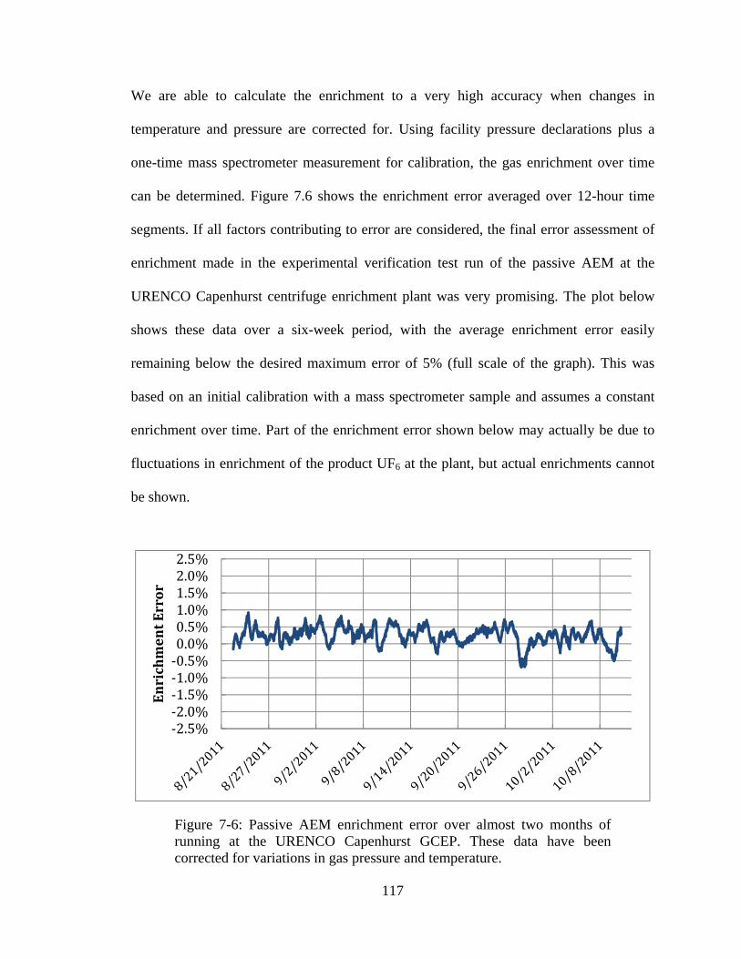
117
We are able to calculate the enrichment to a very high accuracy when changes in
temperature and pressure are corrected for. Using facility pressure declarations plus a
one-time mass spectrometer measurement for calibration, the gas enrichment over time
can be determined. Figure 7.6 shows the enrichment error averaged over 12-hour time
segments. If all factors contributing to error are considered, the final error assessment of
enrichment made in the experimental verification test run of the passive AEM at the
URENCO Capenhurst centrifuge enrichment plant was very promising. The plot below
shows these data over a six-week period, with the average enrichment error easily
remaining below the desired maximum error of 5% (full scale of the graph). This was
based on an initial calibration with a mass spectrometer sample and assumes a constant
enrichment over time. Part of the enrichment error shown below may actually be due to
fluctuations in enrichment of the product UF6 at the plant, but actual enrichments cannot
be shown.
Figure 7-6: Passive AEM enrichment error over almost two months of running at the URENCO Capenhurst GCEP. These data have been corrected for variations in gas pressure and temperature.
‐2.5%‐2.0%‐1.5%‐1.0%‐0.5%0.0%0.5%1.0%1.5%2.0%2.5%
EnrichmentError

118
By averaging the data over 12-hour time segments, the UF6 gas enrichment can be
determined to ±1%. This is well within the limit set by mass balance requirements and if
improved further may even be useful to the plant operators for process control.
119
8 Conclusions
This dissertation has described a method for determining the cascade header pipe
thickness with an enrichment monitor, using an x-ray source and a LaBr3 detector, when
an empty pipe measurement is not feasible. The various possible x-ray filters and isotopic
sources were reviewed, and molybdenum and palladium (with K-edges at 20.0 and 24.35
keV, respectively) were chosen on the basis of initial analytical calculations. These
analytical calculations showed that the ratios of transmitted spectra should be completely
independent of UF6 gas pressure if notch filter thicknesses are optimized.
From the measurements performed, it was determined that notch filters made of a
combination of 0.4-mm palladium and 0.3-mm molybdenum gave the ratio of
transmission spectra that was most independent of UF6 pressure in the pipe. With these
notch filters, a calibration curve was created using our UF6 source with three pipe
thicknesses. This curve allows the pipe thickness to be determined simply by measuring
the ratio of two transmission peak measurements with the two-energy thickness
measurement method. This one-time measurement could be completed in less than an
hour, and once the calibration has been performed for a specific measurement location it
is not necessary to perform it ever again.
When the pipe thickness had been determined, the AEM could be switched to an
unattended mode of operating after selecting an transmission energy that would
maximize transmission through the pipe but still allow measureable attenuation in the
gas. At that point, a single transmission measurement is needed to determine the gas
density, and thus the enrichment. Typically a silver notch filter, with a K-edge at 25.5

120
keV, is used for this purpose. This will be the notch filter used in the next text trial at
Capenhurst, when the active system is installed.
Major issues with the AEM operation that may lead to potential sources of error
in the enrichment determination have been investigated. In order to address these issues,
analytical calculations and experiments have been run to study cascade header pipe-wall
thickness concerns, x-ray tube instabilities, and notch filter material use. This dissertation
briefly looked at the effect of wall deposits on enrichment determination, as well as the
sensitivity of the enrichment results to changes in pressure and temperature during
measurement. In an unfriendly facility, the two-energy thickness measurement method
provides a way to determine the UF6 gas enrichment without using facility pressure
declarations. Alternatively, if facility pressure readings are readily available and can be
trusted, the passive AEM has been shown to produce enrichment results, when corrected,
to within 1% of the actual values.
121
9 Future Work
As a direct follow-on to the work that is ongoing in the URENCO Capenhurst
plant, a field trial is planned for mid-April of this year to install an active AEM system
directly above the passive AEM which is currently installed and collecting data. This
will be the first time an active system, using an x-ray generator as a transmission source,
has been used in an enrichment monitor in a GCEP. The installation will allow a real
analysis of the system performance, because it will be exposed to real temperature
fluctuations and actual changes in gas pressure over the cylinder fill cycles.
One important improvement to the system which will be explored once real data
are acquired is an attempt at performing a running calibration. Using pressure transients
to recalibrate the system will make sure it does not drift over time. These quick (known)
drops in gas pressure when a new cylinder is attached can be periodically used to check
the calibration of the system, and adjust it if needed.
Another possible future path is to look at the whole system – to monitor not only
the GCEP product line, but also to look at the feed and the tails. This could help the
operators monitor their complete process to improve efficiency. It could also be used by
inspectors in the future as a mass balance check (with information from load cells and
other factors) to determine if the input of the system matches the output or whether there
might be diversion taking place.
122
Appendices
Appendix A: Mass Attenuation Coefficients
Appendix B: Equipment Specifications
Appendix C: MCNPX Input File—Diode Flux

123
Appendix A: Mass Attenuation Coefficients
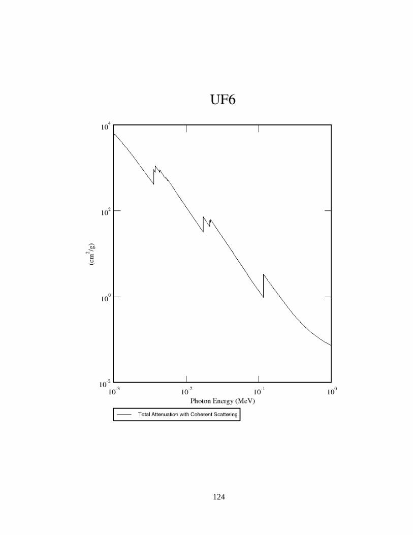
124
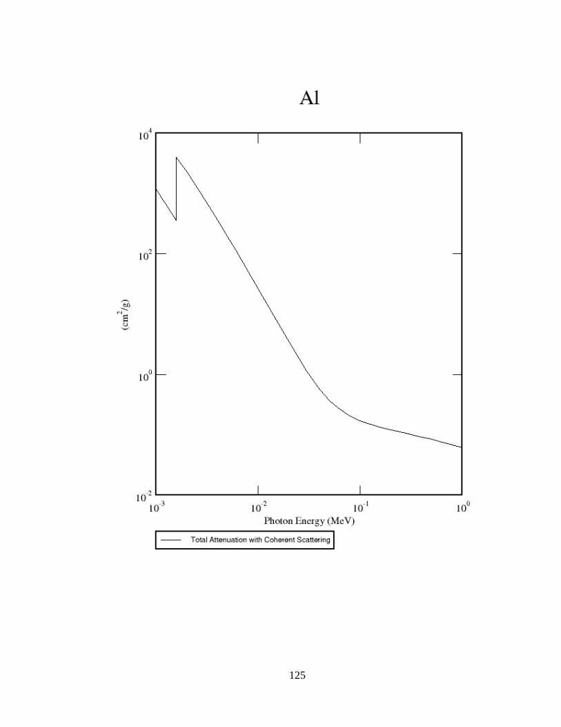
125

126
Appendix B: Equipment Specifications
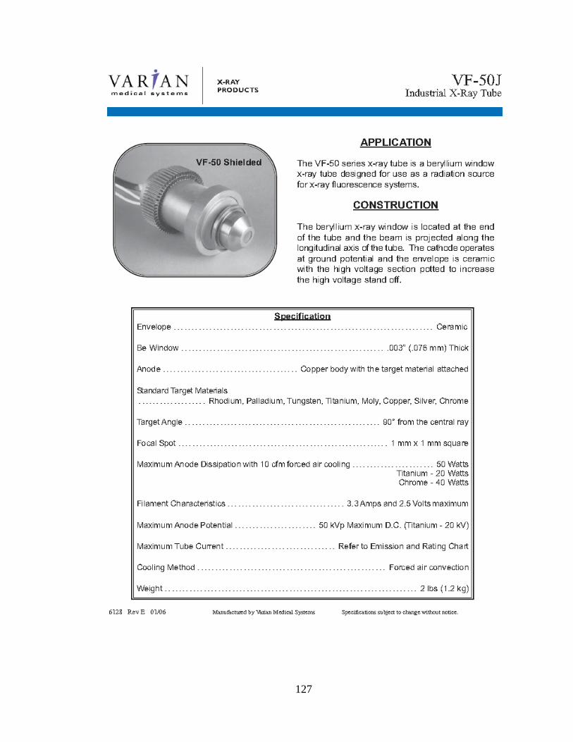
127
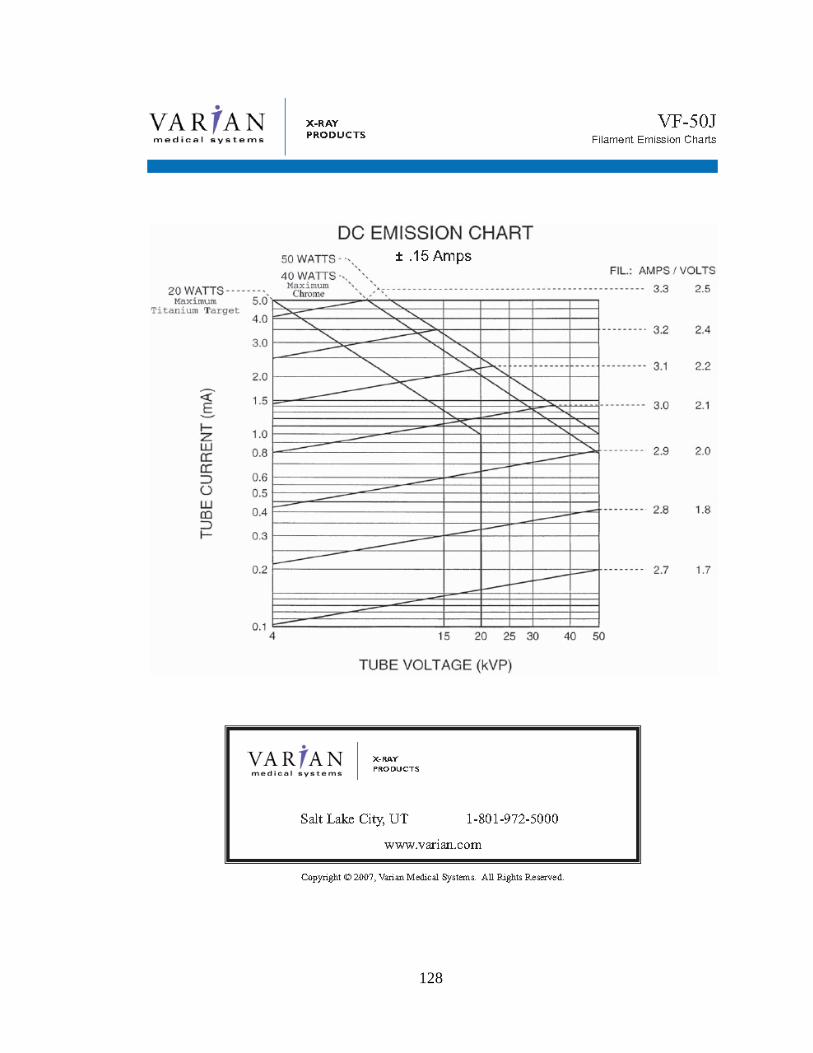
128

129
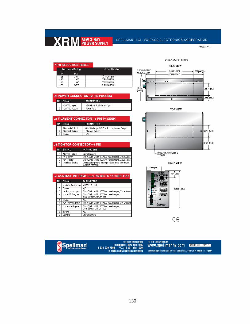
130

131
Appendix C: MCNPX Input File—Diode Flux
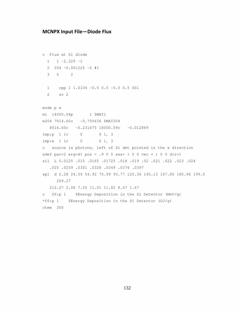
132
MCNPX Input File—Diode Flux
c Flux at Si diode
1 1 -2.329 -1
2 204 -0.001225 -2 #1
3 0 2
1 rpp 1 1.0104 -0.5 0.5 -0.5 0.5 $Si
2 so 2
mode p e
m1 14000.04p 1 $MAT1
m204 7014.60c -0.755636 $MAT204
8016.60c -0.231475 18000.59c -0.012889
imp:p 1 1r 0 $ 1, 3
imp:e 1 1r 0 $ 1, 3
c source is photons, left of Si det pointed in the x direction
sdef par=2 erg=d1 pos = .9 0 0 axs= 1 0 0 vec = 1 0 0 dir=1
si1 L 0.0125 .015 .0165 .01725 .018 .019 .02 .021 .022 .023 .024
.025 .0259 .0301 .0328 .0349 .0376 .0397
sp1 d 2.28 24.59 54.92 75.99 93.77 120.36 145.13 167.80 185.96 199.5
209.27
212.27 2.08 7.55 11.01 11.82 8.47 1.47
c f6:p 1 $Energy Deposition in the Si Detector (MeV/g)
*f6:p 1 $Energy Deposition in the Si Detector (GJ/g)
ctme 300
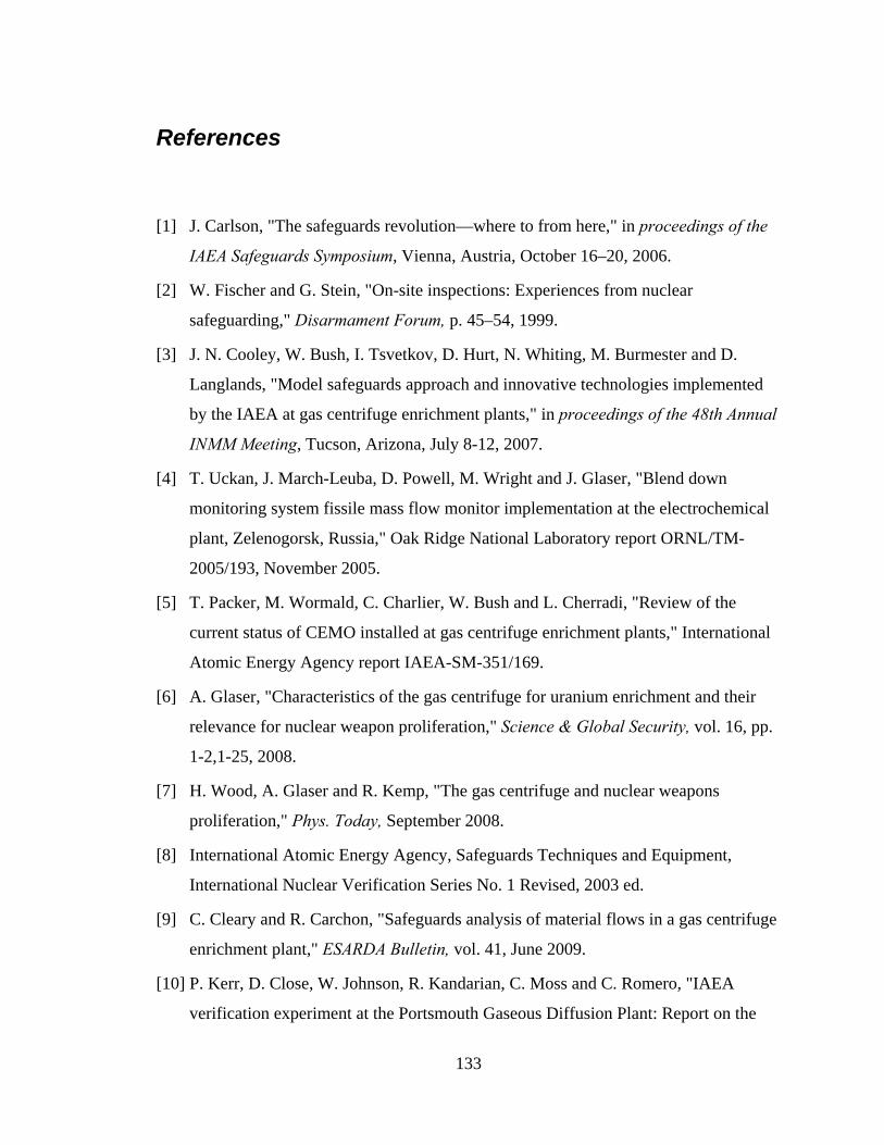
133
References
[1] J. Carlson, "The safeguards revolution—where to from here," in proceedings of the
IAEA Safeguards Symposium, Vienna, Austria, October 16–20, 2006.
[2] W. Fischer and G. Stein, "On-site inspections: Experiences from nuclear
safeguarding," Disarmament Forum, p. 45–54, 1999.
[3] J. N. Cooley, W. Bush, I. Tsvetkov, D. Hurt, N. Whiting, M. Burmester and D.
Langlands, "Model safeguards approach and innovative technologies implemented
by the IAEA at gas centrifuge enrichment plants," in proceedings of the 48th Annual
INMM Meeting, Tucson, Arizona, July 8-12, 2007.
[4] T. Uckan, J. March-Leuba, D. Powell, M. Wright and J. Glaser, "Blend down
monitoring system fissile mass flow monitor implementation at the electrochemical
plant, Zelenogorsk, Russia," Oak Ridge National Laboratory report ORNL/TM-
2005/193, November 2005.
[5] T. Packer, M. Wormald, C. Charlier, W. Bush and L. Cherradi, "Review of the
current status of CEMO installed at gas centrifuge enrichment plants," International
Atomic Energy Agency report IAEA-SM-351/169.
[6] A. Glaser, "Characteristics of the gas centrifuge for uranium enrichment and their
relevance for nuclear weapon proliferation," Science & Global Security, vol. 16, pp.
1-2,1-25, 2008.
[7] H. Wood, A. Glaser and R. Kemp, "The gas centrifuge and nuclear weapons
proliferation," Phys. Today, September 2008.
[8] International Atomic Energy Agency, Safeguards Techniques and Equipment,
International Nuclear Verification Series No. 1 Revised, 2003 ed.
[9] C. Cleary and R. Carchon, "Safeguards analysis of material flows in a gas centrifuge
enrichment plant," ESARDA Bulletin, vol. 41, June 2009.
[10] P. Kerr, D. Close, W. Johnson, R. Kandarian, C. Moss and C. Romero, "IAEA
verification experiment at the Portsmouth Gaseous Diffusion Plant: Report on the
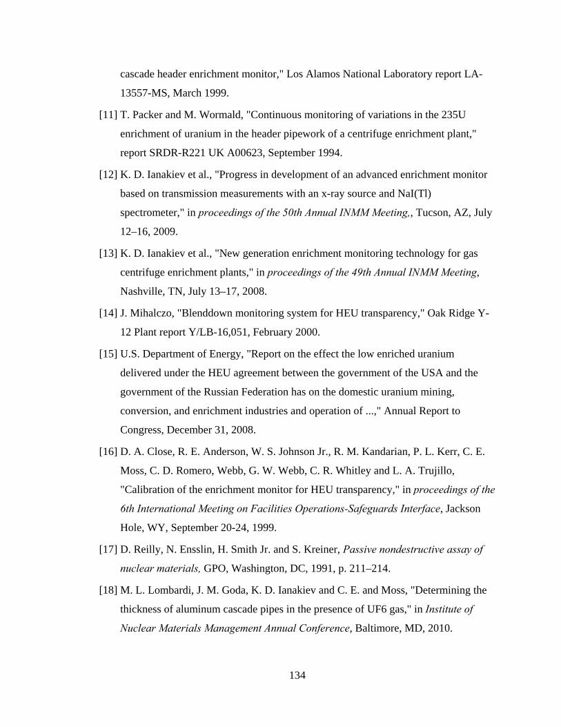
134
cascade header enrichment monitor," Los Alamos National Laboratory report LA-
13557-MS, March 1999.
[11] T. Packer and M. Wormald, "Continuous monitoring of variations in the 235U
enrichment of uranium in the header pipework of a centrifuge enrichment plant,"
report SRDR-R221 UK A00623, September 1994.
[12] K. D. Ianakiev et al., "Progress in development of an advanced enrichment monitor
based on transmission measurements with an x-ray source and NaI(Tl)
spectrometer," in proceedings of the 50th Annual INMM Meeting,, Tucson, AZ, July
12–16, 2009.
[13] K. D. Ianakiev et al., "New generation enrichment monitoring technology for gas
centrifuge enrichment plants," in proceedings of the 49th Annual INMM Meeting,
Nashville, TN, July 13–17, 2008.
[14] J. Mihalczo, "Blenddown monitoring system for HEU transparency," Oak Ridge Y-
12 Plant report Y/LB-16,051, February 2000.
[15] U.S. Department of Energy, "Report on the effect the low enriched uranium
delivered under the HEU agreement between the government of the USA and the
government of the Russian Federation has on the domestic uranium mining,
conversion, and enrichment industries and operation of ...," Annual Report to
Congress, December 31, 2008.
[16] D. A. Close, R. E. Anderson, W. S. Johnson Jr., R. M. Kandarian, P. L. Kerr, C. E.
Moss, C. D. Romero, Webb, G. W. Webb, C. R. Whitley and L. A. Trujillo,
"Calibration of the enrichment monitor for HEU transparency," in proceedings of the
6th International Meeting on Facilities Operations-Safeguards Interface, Jackson
Hole, WY, September 20-24, 1999.
[17] D. Reilly, N. Ensslin, H. Smith Jr. and S. Kreiner, Passive nondestructive assay of
nuclear materials, GPO, Washington, DC, 1991, p. 211–214.
[18] M. L. Lombardi, J. M. Goda, K. D. Ianakiev and C. E. and Moss, "Determining the
thickness of aluminum cascade pipes in the presence of UF6 gas," in Institute of
Nuclear Materials Management Annual Conference, Baltimore, MD, 2010.
135
[19] "Technical White Paper: Bone Densitometry," Conference of Radiation Control
Program Directors, CRCPD publication E-06-5, October 2006.
[20] A. Gotfredsen, L. Baeksgaard and J. Hilsted, "Body composition analysis by DEXA
by using dynamically changing samarium filtration," J. Appl. Physiol., vol. 82, p.
1200–1209, 1997.
[21] C. F. Njeh et al., "Radiological assessment of new bone densitometer – the Lunar
EXPERT," Br. J. Radiol., vol. 69, p. 335–340, April 1996.
[22] S. Clement, A two gamma ray wall thickness gauge for 235U enrichment
measurements, M.S. thesis, University of New Mexico, 1987.
[23] R. M. Cunha e Silva, C. R. Appoloni, P. S. Parreira, F. R. Espinoza-Quino, M. M.
Coimbra and P. H. Aragao, "Two media method for gamma ray attenuation
coefficient measurement of archaeological ceramic samples," Appl. Radiat. and
Isot., vol. 53, p. 1011–1016, 2000.
[24] K. D. Ianakiev et al., "Stability of x-ray tube-based transmission source for UF6 gas
enrichment monitoring technology," in proceedings of the IEEE Nuclear Science
Symposium, Orlando, FL, July 12-16, 2009.
[25] M. Lombardi, J. Goda, K. Ianakiev and C. Moss, "Experimental method for
determining the attenuation by aluminum cascade pipes in the presence of UF6 gas
during enrichment measurements," J. Nucl. Mater. Manage., December 2011.
[26] G. McCall, "Calculation of x-ray bremsstrahlung and characteristic line emission
produced by a Maxwellian electron distribution," J. Phys. D: Appl. Phys., vol. 15, p.
823–831, 1982.
[27] "IRD Website," International Radiation Detectors Inc., [Online]. Available:
http://www.ird-inc.com/. [Accessed 18 January 2012].
[28] "X-Ray Products, VF-50J/S Industrial x-Ray Tube," Varian Medical Systems,
[Online]. Available: http://www.varian.com/media/xray/products/pdf/vf50j.pdf.
[Accessed 18 January 2012].
[29] P. Sprawls, The Physical Principles of Medical Imaging, 2nd Ed., Sprawls
Educational Foundation.
136
[30] "XRM 50W X-Ray Power Supply," Spellman High Voltage Electronics
Corporation, [Online]. Available:
http://www.spellmanhv.com/~/media/Files/Products/XRM.ashx. [Accessed 18
January 2012].
[31] "Absolute X-ray Detectors," International Radiation Detectors, Inc., 15 June 2010.
[Online]. Available: http://www.ird-inc.com/axuvhighnrg.html. [Accessed 18
January 2012].
[32] "Low Current Meters (Picoammeters)," Keithley, 2012. [Online]. Available:
http://www.keithley.com/products/dcac/sensitive/lowcurrent. [Accessed 18 January
2012].
[33] P. Menge, G. Gautier, A. Iltis, C. Rozsa and V. Solovyev, "Performance of large
lanthanum bromide scintillators," Nucl. Instrum. Methods Phys. Res., Sect. A, vol.
579, p. 6–10, 2007.
[34] P. Menge, Performance of Large BrilLanCe 380 (lanthanum bromide) scintillators,
Ann Arbor, MI: SORMI XI, 2006.
[35] "Multichannel Analyzers," ORTEC, 2010. [Online]. Available: http://www.ortec-
online.com/Solutions/multichannel-analyzers.aspx. [Accessed 18 January 2012].
[36] R. DeWitt, "Uranium hexafluoride: A survey of the physico-chemical properties,"
Goodyear Atomic Corporation report GAT-280, Portsmouth, Ohio, August 12, 1960.
[37] A. Favalli, K.D.Ianakiev, C. Keller, M. Lombardi, D. MacArthur, C. McCluskey, C.
Moss and M. Paffett, "Performance evaluation of a multi-detector system for
unattended uranium enrichment monitoring," in proceedings of the INMM 52nd
Annual Meeting, Palm Desert, CA, July 17-21, 2011.
[38] "Photon Cross Sections Database," National Institute of Standards and Technology,
[Online]. Available: http://www.nist.gov/pml/data/xcom/index.cfm. [Accessed 26
January 2012].
[39] "MCNPX," Los Alamos National Laboratory, 26 July 2011. [Online]. Available:
http://mcnpx.lanl.gov/. [Accessed 18 January 2012].
[40] A. Holmes-Seidle and L. Adams, Handbook of Radiation Effects, New York:
137
Oxford University Press Inc., 1993.
[41] B. Rooney, S. Garner and P. Felsher, PeakEasy, Beta Version 3.98 [software], Los
Alamos National Laboratory, 2011.
[42] "THP Home Page," Tungsten Heavy Powder, Inc., [Online]. Available:
http://www.tungstenheavypowder.com/. [Accessed 18 January 2012].
[43] K. Ianakiev, B. Boyer, A. Favalli, J. Goda, T. Hill, C. Keller, M. Lombardi, M.
Paffett, D. MacArthur, C. McCluskey, C. Moss, R. Parker, M. Smith, M. Swinhoe
and P. Friend, "On-line enrichment monitor for UF6 GCEP," in proceedings of the
33rd ESARDA Annual Meeting, Budapest, Hungary, May 2011.
[44] R. Gunnink, NaIGEM Uranium Isotopic Analysis Code for NaI and LaBr3
Detectors, Version 2.1.2 [software], October 2010.
[45] M. Lombardi, A. Favalli, J. Goda, K. Ianakiev, D. MacArthur and C. Moss,
"Experimental determination of the thickness of aluminum cascade pipes in the
presence of UF6 gas during enrichment measurements," Nuclear Instruments and
Methods in Physics Research A, vol. 672, pp. 69-74, 2012.
[46] J. Moore, C. Davis and M. Coplan, Building Scientific Apparatus, Westview Press,
Boulder, Co, 2002.
[47] Alcoa Engineered Products, "Understanding Extruded Aluminum Alloys,"
December 2002. [Online]. Available:
http://www.alcoa.com/adip/catalog/pdf/Extruded_Alloy_6061.pdf. [Accessed 5
December 2012].

138