FRW Cosmology withNon-positively Defined Higgs Potentials

I. Ya. Aref’eva1∗, N. V. Bulatov2†, R. V. Gorbachev1‡

1Steklov Mathematical Institute, Russian Academy of Sciences,

Gubkina st. 8, 119991, Moscow, Russia

2Department of Quantum Statistic and Field Theory, Faculty of Physics

Moscow State University, Leninskie Gory 1, 119991, Moscow, Russia

April 27, 2018

Abstract

We discuss the classical aspects of dynamics of scalar models with non-positiveHiggs potentials in the FRW cosmology. These models appear as effective local modelsin non-local models related with string field theories. After a suitable field redefinitionthese models have the form of local Higgs models with a negative extra cosmologicalterm and the total Higgs potential is non-positively defined and has rather small cou-pling constant. The non-positivity of the potential leads to the fact that on some stageof evolution the expansion mode gives place to the mode of contraction, due to thatthe stage of reheating is absent. In these models the hard regime of inflation givesplace to inflation near the hill top and the area of the slow roll inflation is very small.Meanwhile one can obtain enough e-foldings before the contraction to make the modelunder consideration admissible to describe inflation.

∗arefeva@mi.ras.ru†nick bulatov@mail.ru‡rgorbachev@mi.ras.ru

1

arX

iv:1

112.

5951

v3 [

hep-

th]

21

Mar

201

2

1 Introductory remarks

Scalar fields play a central role in current models of the early Universe – the majority ofpresent models of inflation requires an introduction of an additional scalar – the inflaton[1, 2, 3, 4, 5]. Though the mass of the inflaton is not fixed, typical considerations deal witha heavy scalar field with mass 1013 GeV [6]. The interaction of the inflaton (self-interactingand interacting with matter fields) is not fixed too, moreover, in typical examples the self-interaction potential energy density of the inflaton is undiluted by the expansion of theuniverse and it acts as an effective cosmological constant. However the detailed evolutiondepends on the specific form of the potential V . In the last years, in particular, Higgsinflation has attracted a lot of attention [9]-[14]. The kinetic term usually has the standardform, however models with nonstandard kinetic terms also have attracted attention in theliterature [15]-[17]. The present paper deals with models mainly related with a nonlocalkinetic term of a special form [17]-[38].

The distinguish property of these models is their string field (SFT) origin [39]. Theoriginal motivation to deal with this type of nonlocal cosmological models was related withthe dark energy problems [17]. The relevance of this type of models to the early Universeproblems has been pointed out in [25, 26]. In this case the scalar field is the tachyon of theNSR fermion string and the model has the form of a nonlocal Higgs model. These nonlocalfactors produce essential changes in cosmology. Due to the effect of stretching the potentialwith the kinetic energy advocated by Lidsey[25], Barnaby and Cline[26] nonlocality destroysthe relation between the coupling constant in the potential, the mass term and the value ofthe vacuum energy (cosmological constant) and produces the total Higgs potential with thenegative extra cosmological term. This total Higgs potential is non-positively defined.

We discuss the classical aspect of dynamics of scalar models with non-positive Higgspotentials in the FRW cosmology. As it has been mentioned above these models appear aseffective local models in nonlocal models of a special form related with string field theory.

Since nonlocality can produce an effective local theory with rather small coupling constantsome stages of evolution can be described by the free tachyon approximation. Due to thisreason we start from consideration of dynamics of the free tachyon in the FRW metric. Weshow that generally speaking there are 4 stages of evolution of the tachyon in the FRWmetric: reaching the perturbative vacuum from the past cosmological singularity; rollingfrom the perturbative vacuum; transition from inflation to contraction and in the endingcontraction to the future cosmological singularity. We present approximations suitable tostudy evolution near the past cosmological singularity, evolution near the top of the hill andevolution near the transition from expansion to contraction.

As to the case of the quartic potential the situation depends on the constant relations.For very small coupling constant the hard regime of inflaton gives place to inflation nearthe hill top making the area of the slow-roll inflation very small. Meanwhile the model canperform enough e-foldings to make the model under consideration admissible do describeinflation.

The plan of the paper is the following. We start, Sect. 2.1, from the short expositionwhy the nonlocality of the SFT type produces non-positively defined potentials. In Sect.2.2 we remind the known facts about massive scalar field and the positively defined Higgs

2

potential.In Sect.3 we consider dynamics of the free tachyon in the FRW metric. First, we show

the presence of the cosmological singularity [51]. Then we show that starting from thetop of the hill the tachyon first evolves as an inflaton, i.e. it keeps the inflation regime.After performing a finite number of e-foldings Nmax the tachyon reaches the boundary ofthe forbidden domain at some point (φmax, φmax) of the phase diagram. At this point theHubble H becomes equal to zero and the tachyon continues to evolve with negative H, i.e.the tachyon becomes in fact a “contracton”. We study the phase portrait of the system andconclude that near the top we can use the de Sitter approximation and, moreover, we canrestrict ourself to consideration of one mode of the tachyon evolution, so called C1-mode,and find corrections to the dS approximation. This regime has been previously studied in[40, 42]. The C1-mode is a more viable mode and in the case of the zero cosmological constantdescribes exponentially increasing solution at t→∞. To study dynamics of the system nearthe boundary of the accessible area in more details we use a special parametrization, that is infact a generalization of a parameterizations that one has used previously to study dynamicsof the inflaton with a positively defined potential in the FRW metric [51] and refs. therein.Using this parametrization we find asymptotic behavior near the boundary of the accessibleregion.

In Sect.4 we consider dynamics of the Higgs field in the FRW metric in the presence of anextra negative cosmological constant. This constant makes the total potential non-positivelydefined and produces the forbidden area in the phase space of the Higgs field.

In conclusion we briefly summarize new cosmological features for Higgs potentials withextra negative cosmological constant. The perturbation analysis will be the subject of for-going paper.

2 Setup

2.1 Non-positively defined potentials as a consequence of nonlo-cality

In this section we make few remarks why scalar matter nonlocality leads to essential changesof properties of corresponding cosmological models in comparison with those of pure localcosmological models (we mean early cosmological models). These changes appear due to aneffective stretch of the kinetic part of the matter Lagrangian.

We deal with the nonlocal action originated from SFT [17]

S =

∫d4x√−g[m2p

2R +

(1

2φ(ξ2 + µ2)e−λφ− V (φ)− Λ

)], (2.1.1)

where is the D’Alembertian operator, ≡ 1√−g∂

µ(√−g∂µ), φ is a dimensionless scalar

field and all constants are dimensionless.The spatially isotropic dynamics of this field in the FRW metric, with the interval:

ds2 = − dt2 + a2(t)(dx2

1 + dx22 + dx2

3

),

3

is given by nonlocal equation of motion

eλ(∂2+3H∂)(ξ2(∂2 + 3H∂)− µ2

)φ(t) = −V ′φ, (2.1.2)

3H2 = 8πG E , (2.1.3)

where the Hubble parameter H = a/a, E is a sum of nonlocal modified kinetic and potentialenergies, that are explicit functionals of φ and φ. E is given by [17]-[33] (see also [47]-[49])

E = 2E00 − g00 (gρσEρσ +W ) ,

where

E00 ≡1

2

∞∑n=1

λn

n!

n−1∑l=0

∂0lgφ∂0

n−1−lg φ,

W ≡ 1

2

∞∑n=2

λn

n!

n−1∑l=1

lgφ

n−lg φ+

f0

2φ2 + V (φ).

In the main consideration we deal with V (φ) = εφ4 and f0 = −µ2 (the tachyon case).In comparison with the local scalar field dynamics in the FRW metric

φ+ 3Hφ = −V ′φ, (2.1.4)

3H2 = 8πG(1

2φ2 + V (φ)), (2.1.5)

there are two essential differences: there is a nonlocal kinetic term in the equation forscalar field (2.1.2) as well as the form of the energy is different. Generally speaking thesystem (2.1.2), (2.1.3) is a complicated system of nonlocal equations and its study is a rathernontrivial mathematical problem. There are several approaches to study this system. Let usfirst mention the results of study of equation (2.1.2) in the flat metric, i.e. equation (2.1.2)with H = 0. In the flat metric for the quartic potential it is known that for ξ < ξc thereexists an interpolating solution of (2.1.2) between two vacua1. There is a numerical evidencefor existence of oscillator solutions for ξ > ξc. In the LHS of (2.1.2) there is a nonlocal termthat is related with the diffusion equation. This relation provides rather interesting physicalconsequences [50].

The case of the FRW metric in the context of the DE problem has been studied in[17, 20, 28, 29]. In the context of the inflation problem this system (especially in the caseξ = 0) has been studied in [25, 26]. In [25] it has been pointed out that nonlocal operatorslead to the effects that can be quantified in terms of a local field theory with a potentialwhose curvature around the turning point is strongly suppressed.

In the case of a quadratic potential a cosmological model with one nonlocal scalar fieldcan be presented as a model with local scalar fields and quadratic potentials [22, 23, 24,29, 34, 36, 37]. For this model it has been observed [25, 26] that in the regime suitable forthe Early Universe the effect of the effective stretch of the kinetic terms takes place (see

1There is no interpolating solution for the case of cubic potential [47].

4

also [24, 29]). One can generalize this result to a nonlinear case and assume that a nonlocalnonlinear model can be described by an effective local nonlinear theory with the followingenergy density

E ≈ eλΩ2

(1

2φ2 − 1

2µ2φ2

)+

1

4εφ4 + Λ, (2.1.6)

and the tachyon dynamics equation becomes

∂2φ+ 3H ∂φ− µ2φ = −εe−λΩ2

φ3, (2.1.7)

where

H =1√

3mp

√eλΩ2

(1

2φ2 − 1

2µ2φ2

)+

1

4εφ4 + Λ (2.1.8)

and we take ξ = 1 for simplicity. Ω is a modified “frequency” of the asymptotic expansionfor equation (2.1.7) in the flat case. In the first approximation Ω = µ.

Or in other words, one can say that the higher powers in cause the factor eλΩ2, where

Ω2 in the first approximation is just equal to µ2. Therefore, the corresponding effectiveaction becomes

S =

∫d4x√−g[m2p

2R +

(1

2φ( + µ2)eλΩ2

φ− εφ4

4− Λ

)]. (2.1.9)

In term of the canonical field ϕ ≡ eλΩ2/2φ the action (2.1.9) becomes

S =

∫d4x√−g[m2p

2R +

(1

2ϕ( + µ2)ϕ− ε

4e−2λΩ2

ϕ4 − Λ

)]. (2.1.10)

Just this form is responsible for equation (2.1.7) for V (φ) = − εφ4

4. This equation is nothing

more than equation for the Higgs scalar field considered as an inflaton. There is only onedifference, that in fact, as we will see, is very important. The potential for the Higgs modelbeing considered usually in the context of the cosmological applications is

V (φ) =ε

4(φ2 − a2)2, (2.1.11)

i.e. the cosmological constant Λ = ε4a4 is such that the potential is the positively defined

potential. Let us remind that in the SFT inspired nonlocal model the value of the cosmolog-ical constant is also fixed by the Sen conjecture [39, 43, 44] that exactly puts the potentialenergy of the system in the nontrivial vacua equal to zero

V (φ) = −1

2µ2φ2 +

1

4εφ4 + Λ =

1

4ε

(φ2 − µ2

ε

)2

, (2.1.12)

that gives us he value of Λ = µ4

4ε. The appearance of the extra factor eλΩ2

destroys thispositivity

VEL(φ) = −1

2µ2eλΩ2

φ2 +1

4εφ4 +

µ4

4ε=

1

4ε

(φ2 − µ2

εeλΩ2

)2

+µ4

4ε

(1− e2λΩ2

), (2.1.13)

(here ”EL” means ”effective local model”). Since λ > 0, we have to deal with non-positivelydefined potential.

5

2.2 Phase portraits for positively defined potentials

Cosmological models with one scalar field with positively defined potential are well studiedmodels, see for example [2, 51, 54, 55, 56]. Let us remind the main features of the phaseportraits of these models. The phase portrait for a free massive field that is a solution of

φ+ 3

√8πG

3

(1

2φ2 +

m2

2φ2

)φ = −m2φ, (2.2.1)

is presented in Fig.1.A. The same phase portrait is presented in Fig.1.B in compactifiedvariables. The advantage of this picture is that we see the existence of the cosmologicalsingularity. The phase portrait for the Higgs field with positively defined potential

φ+ 3

√8πG

3

(1

2φ2 +

ε

4(φ2 − a2)2

)φ = −εφ3 + εa2φ, (2.2.2)

is presented in Fig.2.A.

A. B.

Figure 1: (color online) A. The phase portrait of equation (2.2.1). B. Inflaton flows incompactified variables ψ vs ρ are given by the phase portrait of equations (2.2.6) and (2.2.7).

Comparing the inflaton flows in Fig.1.A, Fig.2.A, we see that there is no big differencebetween the phase portrait presenting the chaotic inflation (2.2.1) and the phase portrait ofeq. (2.2.2). This is in accordance with the general statement about a weak dependence ofthe inflaton flow on the potentials. Only explicit formulae describing the slow-roll regimeas well as the oscillation regime are different. In all these cases there are 3 stages (eras) ofevolution. Just after cosmological singularity the ultra-hard regime starts. Then in the caseof any positive/negative initial position φ(0) > 0/φ(0) < 0 the inflaton reaches very fast the“right”/“left” attractor. Then the inflaton moves along the “right”/“left” slow-roll line. Inparticular, in Fig.1.A there is almost horizontal line that corresponds to the “right” slow-roll

6

A. B.

Figure 2: (color online) A. The phase portrait of equation (2.2.2). B. The Phase portraitof the system of equations (2.2.8), (2.2.9).

line and it is seen in the plot as a common part of the red, pink and magenta lines. Thenoscillations near the point φ = 0, φ = 0 Fig.1.A, or near one of two nonperturbative vacuaFig.2.A start.

It is well known that it is convenient to present the phase portraits in the compactifiedvariables [51] (G = 1

m2p)

φ =3mp√12π

ρ

1− ρsin θ cosψ, (2.2.3)

φ =3mmp√

12π

ρ

1− ρsin θ sinψ, (2.2.4)

H = mρ

1− ρcos θ. (2.2.5)

With the help of these variables we can rewrite equations (2.2.1) and H = −4πφ2

m2p

in the

following form (here we use the time variable σ such that dσdτ

= 11−ρ where τ = mt)

ρσ = −3ρ2(1− ρ)√2

sin2 ψ, (2.2.6)

ψσ = −(1− ρ)− 3ρ

2√

2sin 2ψ, (2.2.7)

7

and equation for the Higgs inflaton (2.2.2) has the form (g =3m2

p

4πa2)

ρσ = (1− ρ)2ρ sin2 θ sin 2ψ − ρ2(1− ρ) cos θ(1 + 4 sin2 θ sin2 ψ

)(2.2.8)

+1

2g(1− ρ)3 cos θ + gρ3 sin4 θ cos3 ψ

(ρ

1− ρcosψ cos θ − sinψ

),

ψσ = −3

2ρ cos θ sin 2ψ + (1− ρ) cos 2ψ − g ρ2

1− ρsin2 θ cos4 ψ. (2.2.9)

θσ = (1− ρ) sin 2ψ sin 2θ − 1

2g

(1− ρ)2

ρsin θ + ρ sin θ

[1− 3 sin2 ψ

+ 2 sin2 ψ sin2 θ]− g ρ2

1− ρsin3 θ cos3 ψ

[sinψ cos θ +

ρ

1− ρsin2 θ cosψ

](2.2.10)

Phase portraits for systems of equations (2.2.6), (2.2.7) and (2.2.8), (2.2.9) are presentedin Fig.1.B. and Fig.2.B.

3 Free Tachyon in the FRW space

3.1 The exact phase portrait of the free tachyon

The dynamics of the free tachyon in the FRW metric corresponding to the expansion (H > 0)is described by the following equation

φ+ 3

√8πG

3

(1

2φ2 − µ2

2φ2 + Λ

)φ = µ2φ. (3.1.1)

The phase portraits of eq. (3.1.1) is presented in Fig.3.A. We see that there are two forbiddenregions in the phase space. The distance between these forbidden regions depends on thevalue of the cosmological constant. The boundary of the accessible domain is given by therelation φ = ±

√µ2φ2 − 2Λ. The accessible region is divided by 4 domains, I, II, III and

IV, that are separated by two separatrices: S1 and S2, see Fig.3.A. The upper half of theseparatrix S1 is an attractor (the “right” attractor), and the low part of the separatrix S1 isthe other attractor (the “left” attractor). The separatrix S2 consists of two repulsers.

In Fig.3.A. we see several eras of the tachyon evolution. Let us consider trajectoriesstarting at region I. First, the tachyon reaches the area of the right attractor. In particular,starting from zero initial value φ(0) = 0 (the corresponding trajectories are presented inFig.3.A. by colored lines) the tachyon decreasing the value of H reaches the area near theboundary of the accessible domain, where H = 0. In Fig.4.A. the lines with fixed positivevalues of H are denoted by the blue dashed lines. In Fig.4.B we present the 3d plot of valuesof H depending on the position in the phase diagram. In the end of this era of evolution thetachyon reaches the line corresponding to H = 0. Then the tachyon keeps moving in thearea of the negative H, see Fig.3.B, regions V and VI. Therefore, starting at region I thetachyon continues its evolution in region V. The tachyon EOM in regions V and VI has the

8

S1

S2

II

III

I

IV

1

2

3

4

5

φ

φ

A.VI

V

1′2′

3′

4′

5′

φ

φ

B.

Figure 3: (color online) A. The phase portrait of equation (3.1.1). The accessible regionis divided by 4 domains, that are separated by two separatrices: S1 (the red dotted line)and S2 (the magenta dotted line). Colored lines present trajectories starting from differentpoints of the phase diagram. B. The phase portrait of equation (3.1.2). Continuations of thetrajectories presented in the left panel to solutions of the Friedman equation with negativevalues of H are indicated by the same numbers with primes added.

form

φ− 3

√8πG

3

(1

2φ2 − µ2

2φ2 + Λ

)φ = µ2φ. (3.1.2)

We see from the phase portrait Fig.3 that for finite φ and φ there are no critical points.To search for critical points in the infinite phase space as well as to justify approximationsin different domains of the phase space (in particular, in neighborhood of the forbiddendomains) it is convenient following to [51] to rewrite the scalar field equation in FRW space-time as a system of equations for 3-dimensional dynamical system. There are two types ofslightly different recipes how to do this. One is given in [51] and uses variables (3.3.2)-(3.3.4)(see below) and the second one is given in [53] for positively defined potentials and is givenby formula (3.7.1)-(3.7.3). The first recipe is convenient to study the cosmological singularity(see sect.3.3) and the second one – to study a transition from expansion to contraction (seesect.3.7)

3.2 Free Tachyon in FRW in the slow-roll regime

In the slow-roll regime one usually ignores the second derivative of the field on time in theequation of motion and the kinetic term in the equation for H. In this case the tachyonequation becomes

3

√8πG

3

(Λ− µ2

2φ2

)φ = µ2φ. (3.2.1)

9

A. B.

Figure 4: (color online) A. The same phase portrait as in Fig.3.A. with marked lines (dashedblue lines) of the constant values of H. The thick dashed line corresponds to H2 = 3κΛ(κ = 8πG

9). The solid blue line corresponds to H = 0 and defines the boundary of the

accessible domain. B. The plot of the functional κ(12ψ2 − µ2

2φ2 + Λ) that defines the value

of H2 (here φ = ψ). The intersection with the yellow plane corresponds to the boundary ofthe accessible region.

This equation obviously has a meaning only for

|φ| <√

2Λ

µ.

According to the common approach we can use the slow-roll approximation when slow-rollparameters ε and η are very small

ε =m2p

16π

(V ′

V

)2

1,

|η| =

∣∣∣∣m2p

8π

(V ′′

V

)∣∣∣∣ 1.

We can see the typical behaviour of these parameters for the model being considered inFig.5 A and B in the case when the slow-roll conditions are satisfied. As we see in someinterval of φ values near 0 the slow-roll parameters are small enough. That means that one

10

A. B.

C. D.

Figure 5: (color online) A. The dependence of slow-roll parameter ε on φ in the case whenthe slow-roll conditions are satisfied. B. The dependence of slow-roll parameter η on φ in thecase when the slow-roll conditions are satisfied. C. The phase portraits for the model whenthe slow-roll conditions are satisfied on some interval of φ values near 0. The green solidlines correspond to different exact trajectories, the blue dashed and dot line corresponds tothe slow-roll trajectory. D. The zoomed part of the Fig.C near (0,0) where the slow-rollconditions are highly satisfied.

11

should expect a good approximation of slow-roll solution for the exact phase trajectories onthis interval.

We can see in the phase portraits shown in Fig.5 C and D that really in this case onsome interval of φ values near 0 the exact phase trajectories are close enough to the slow-roll trajectory. When the slow-roll parameters become large enough we see the differencebetween the exact trajectories and the slow-roll trajectory.

In the case when the slow-roll conditions are not satisfied the slow-roll parameters evolveas it’s shown in Fig.6 A and B. The phase portraits for this case are shown in Fig.6 C andD. As we see the exact trajectories cross the slow-roll trajectory but don’t keep on evolvingalong it. It means that the slow-roll approximation really cannot be used for the descriptionof the exact trajectories in this case. We can note that in the region where φ is small enoughthe minima of the exact phase trajectories are situated on the slow-roll trajectory. It isconnected with the fact that the minimum of the exact phase trajectory corresponds to thepoint where φ = 0 and if we also can neglect φ in the expression for H then from the exactequation of motion we obtain the point of the slow-roll trajectory.

3.3 Tachyon dynamics near cosmological singularity

To study tachyon dynamics near the cosmological singularity let us consider for simplicitythe case of the zero cosmological constant

φ+ 3

√8πG

3

(1

2φ2 − µ2

2φ2

)φ = µ2φ. (3.3.1)

This approach is valid when φ and φ are large enough.In terms of dimensionless variables

X =

√12π

3mp

φ, (3.3.2)

Y =

√12π

3µmp

φ, (3.3.3)

Z =H

µ, (3.3.4)

τ = µt, (3.3.5)

system (3.3.1) has the form

Xτ = Y, (3.3.6)

Yτ = +X − 3ZY, (3.3.7)

Zτ = −X2 − 2Y 2 − Z2. (3.3.8)

12

A. B.

C. D.

Figure 6: (color online) A. The dependence of slow-roll parameter ε on φ in the case whenthe slow-roll conditions are not satisfied. B. The dependence of slow-roll parameter η on φ inthe case when the slow-roll conditions are not satisfied. C. The phase portraits for the modelwhen the slow-roll conditions are not satisfied. The green solid lines correspond to differentexact trajectories, the blue dashed and dot line corresponds to the slow-roll trajectory. D.The zoomed part of the Fig.C near (0,0).

13

To get compactification of the phase space we use the coordinates of the unit ball

X =ρ

1− ρsin θ cosψ, (3.3.9)

Y =ρ

1− ρsin θ sinψ, (3.3.10)

Z =ρ

1− ρcos θ, (3.3.11)

and in these new coordinates the equation of motion takes the form

ρσ = ρ(1− ρ)2

[sin 2ψ sin2 θ − ρ

1− ρcos θ

(1 + 4 sin2 ψ sin2 θ

)], (3.3.12)

ψσ = −3

2ρ sin 2ψ cos θ + (1− ρ) cos 2ψ, (3.3.13)

θσ =1

2(1− ρ) sin 2ψ sin 2θ + ρ sin θ

(1 + sin2 ψ − 4 cos2 θ sin2 ψ

), (3.3.14)

heredσ

dτ=

1

1− ρ.

This system has 4 critical points with ρ = 1 lying on the cone

Y 2 = X2 + Z2,

that in the spherical coordinates has the form

tan2 θ = − 1

cos 2ψ. (3.3.15)

These critical points are

θ0 =π

4, ψ0 =

π

2, (3.3.16)

θ0 =π

4, ψ0 = −π

2, (3.3.17)

θ0 =3π

4, ψ0 =

π

2, (3.3.18)

θ0 =3π

4, ψ0 = −π

2. (3.3.19)

Let us now consider the behavior of the system near the critical point (3.3.16), i.e.ρ = 1, θ0 = π

4, ψ0 = π

2. The have near this point in the linear approximation

d

dσ∆ρ (σ) =

3

2∆ρ (σ)

√2, (3.3.20)

d

dσ∆ψ (σ) = −∆ρ (σ) +

3

2

√2∆ψ (σ) , (3.3.21)

d

dσ∆θ (σ) = 2

√2∆θ (σ) . (3.3.22)

14

A. B.

Figure 7: (color online) A. The 3-dimensional picture of the dynamics of the tachyon(system of equations (3.3.12)-(3.3.14)). We see that all trajectories starting on the conuskeep moving on the conus. The red parts of trajectories correspond to the expansion andthe blue part to the contraction. B. The projection of the previous picture on the XY -plane.This picture is the tachyon analogue of the picture for the free particle in the FRW presentedin the Fig.1

The eigenvalues are (32

√2, 3

2

√2, 2√

2), and solutions to this system are

∆ρ (σ) = C2 e32

√2σ, (3.3.23)

∆ψ (σ) = (C1 − C2σ)e32

√2σ, (3.3.24)

∆θ (σ) = C3 e2√

2σ. (3.3.25)

3.4 Approximation of tachyon dynamics in the FRW by dynamicsin the dS space

During the evolution of the tachyon between two dashed lines, see Fig.4.A, corresponding toH = H0 ±∆H0, we can ignore the dependence of H on time and we take an approximate

φ+ 3H0 φ = µ2φ. (3.4.1)

Near the thick blue dashed line we can use

H0 =

√8πG

3Λ, (3.4.2)

and near the starting point with given φ0 and φ0 we can use the approximation

H0(φ20, φ

20) =

√8πG

3

(1

2φ2

0 −µ2

2φ2

0 + Λ

).

15

In Fig.8.A we present the phase diagram for the tachyon evolution in the dS space,equation (3.4.1). We see that there are two attractors and two repulsers. The phase portraitsfor dynamics of the tachyon in the dS space with two different Λ are presented in Fig.8.Bby blue and magenta vectors (the blue vectors for small Λ and the magenta vectors for largeΛ).

A. B.

Figure 8: (color online) A. The phase portrait of the tachyon evolving in the dS space. Thereare two attractors and two repulsers. B. A comparison of the tachyon phase portraits in thedS space with different Λ (the blue vectors for small Λ, the magenta vectors for large Λ). Theblue/cyan and red/pink solid lines present the dynamics of the tachyon with the same initialdata in the dS space-time with different values of the cosmological constant Λ. The blue/redand cyan/pink lines have the same initial coordinates, but different initial velocities.

Equation (3.4.1) has solutions

φ(t) = C1 er+t + C2 e

r−t, (3.4.3)

where

r± = −3

2H0 ±

3

2

√H0

2 +4

9µ2, (3.4.4)

i.e. r+ > 0, r− < 0. We see that for H0 > 0 the C2-mode decreases faster in comparisonwith the C1-mode that increases for large t.

For the initial date φ(0) = 0 we have

φ (t) = C e−3/2H0t sinh

(3H0

2

√1 +

4

9

µ2

H20

t

), C1 = C/2 (3.4.5)

and

limt→∞

φ (t)

φ(t)= −3

2H0 +

3H0

2

√1 +

4

9

µ2

H20

. (3.4.6)

16

This is exactly the same answer if we keep only the first term in (3.4.3). One can saythat C1-mode is an attractor for all solutions of the tachyon dS equation with zero initialcoordinates. C1-mode is important for large times, but we cannot ignore the C2-mode forsmall times. We also see that the C1-mode is a dominating mode for t > 0 for the case whenH0 = 0. One can say that the C1-mode is a viable mode and the C2-mode is a transient one.

To select the C1-mode one can also assume that one deals with the solution such as ifthe tachyon was sitting on the top of the hill at t = −∞.

Let’s note that the C1-mode corresponds to the slow-roll trajectory on the interval wherewe can consider H as an approximate constant. It means that the slow-roll trajectory is aquasi-attractor for the exact trajectories.

To illustrate how the approximation (3.4.1) works, in Fig.9 we compare phase portraitsfor equations (3.1.1) and (3.4.1). We see that for small times and small initial velocities theapproximation works, but it is failed for large times

A. B.

Figure 9: (color online) A. A comparison of the exact evolution (numerical solution of eq.(3.1.1)) with an approximate evolution (3.4.1) with H0 given by (3.4.2). The solid green andkhaki lines in the left panel represent the exact trajectories and the blue and cyan dashedlines represent the approximate trajectories. Magenta vectors in the left panel represent thephase portrait of the exact equation. Blue vectors in the right panel represent the phaseportrait in the dS space. B. The solution and the phase portraits for the approximateequation.

To estimate a deviation of H from the initial H0 we calculate the energy of solution(3.4.3) of the tachyon equation in the dS space-time. The energy of this solution is a sum ofthe energies of two modes [24]

E = EC1 + EC2 ,

17

where

EC1 =1

2φ2C1− µ2

2φ2C1

= C21

9

4H2

0

(1−

√1 +

4

9

µ2

H20

)e2r+t, (3.4.7)

EC2 =1

2φ2C2− µ2

2φ2C2

= C22

9

4H2

0

(1 +

√1 +

4

9

µ2

H20

)e2r−t. (3.4.8)

We see that C1 gives a negative contribution to the energy and C2-mode gives a positiveone. Since the C1-mode is more viable mode its negative energy contribution dominates andthe tachyon loses the initial energy in the FRW space up to zero value.

3.5 Inflation over the hill

In this subsection we remind the consideration of a scalar field rolling over the top of alocal maximum of a potential following the paper by Tzirakis and Kinney [42]. This evo-lution needs a special attention as it cannot be considered in framework of the slow-rollapproximation. It follows from the fact that in the slow-roll limit

φ ∝ V ′ (φ) = 0,

at the maximum of the potential.The tachyon equation (3.4.1) can be rewritten in terms of the number of e-foldings N,

N ≡ ln a/ainitial (we omit ainitial) as

φ′′ + 3φ′ = ν2φ, (3.5.9)

where ν2 = µ2

H20

and φ′ = dφdN

. The general solution of (3.5.9) is

φ(N) = φ+eν+N + φ−e

ν−N , (3.5.10)

with ν± = −32(1∓

√1 + 4

9ν2). This form of the tachyon evolution is just the reparametriza-

tion of (3.4.3).If ν2 is small, the constants ν± become in the first approximation

ν+ =ν2

3,

ν− = −3− ν2

3.

(3.5.11)

As in the previous consideration the general solution (3.5.10) can be decomposed intotwo branches: a transient branch ν− which dominates at early times, and a “slow-rolling”branch ν+ which can be identified as the late-time attractor.

If we consider these branches separately we see that the slow-roll parameters are [42]

ε = 4πν2±

(φ

mp

)2

,

η = −ν± + ε.

(3.5.12)

18

Near the maximum of the potential being considered, φ ≈ 0 and ε 1, so that

η ≈ −ν± = constant. (3.5.13)

Even though we assume ε to be small, it is obvious from eqs. (3.5.11) and (3.5.13) that theν− branch will never satisfy the slow -roll conditions, since η > 3 always. For the ν+ branch,the slow-roll limit is obtained for ν 1 for which

|ηSR| ≈ν2

3 1.

It was also shown in [42] that ν− branch corresponds to a field rolling up the potential.If we consider the whole solution (3.5.10) we see that in order for the field to be a

monotonic function of time, its derivative must not change a sign. It means

dφ

dN= ν+φ+e

ν+N + ν−φ−eν−N 6= 0, (3.5.14)

we assume that the derivative of the field with respect to N is a smooth function throughoutits evolution. Since we know the signs of the constants ν±, the above condition can beachieved only if one of the coefficients φ± is negative. If we take φ− < 0, it will result in apositive time derivative for the field

φ = Hdφ

dN> 0.

If here we consider the field rolling over the hill then at some moment when N = N0 thefield must get the value equal to 0 that corresponds to the maximum of the potential. Itmeans that

φ+eν+N0 = −φ−eν−N0 .

We can rewrite the expression for the general solution as follows

φ = A[eν+(N−N0) − eν−(N−N0)

],

whereA = φ+e

ν+N0 = −φ−eν−N0 .

As we see in the left part of potential the ν− branch dominates that means that slow-rollapproximation cannot be used in this region and after rolling over the top the ν+ branchdominates and slow-roll mode can start if necessary conditions are satisfied.

In the next subsection we consider the next approximation of the tachyon in the FRWmetric.

3.6 Next-to-leading terms in the approximate dynamics of thetachyon in the FRW metric

Starting from the dS approximation, H = H0, where H0 is given by (3.4.2), and selectingthe C1-mode one can find a solution of equation (3.1.1) performing an analytical expansion

19

in powers of the C1-mode [21, 26, 30],

φ(t) =∞∑n=1

φnenr+t, (3.6.15)

H(t) = H0 −∞∑n=1

Hnenr+t. (3.6.16)

In the next to the leading approximation

H(t) = H0 −H2e2r+t + ... (3.6.17)

with

H2 = −3πGφ21H0

(1−

√1 +

4

9

µ2

H20

). (3.6.18)

In this approximation the tachyon equation (3.1.1) has the form

φ+ 3(H0 −H2e2r+t) φ = µ2φ (3.6.19)

and expanding the solution in the series (3.6.15) we get

φpert.sol(t) ≈ φ1er+t + φ3e

3r+t + ..., (3.6.20)

where

φ3 =3H2

8r+ + 6H0

φ1. (3.6.21)

Note that the denominator in (3.6.21) has no zeros.Note also that in the accepted scheme of calculation we get an one-parametric set of

solutions and we deal only with the more viable mode. We can check this explicitly. To thispurpose we note that the general solution to (3.6.19) has the form

φ(t) = (c1M(a, a, x) + c2W(a, a, x)) ex2 e−2ar+t, (3.6.22)

where M is the Whittaker M function and W is the Whittaker W function and

a =2 r+ + 3H0

4r+

=

√9H2

0 + 4µ2

4r+

, x =3H2e

2 r+t

2r+

.

Using the relation of the Whittaker function with the hypergeometrical functionΦ(α, β, z) ≡1 F1(α, β, z) we get

φ(t) = er+t

(c1

(3H2

2r+

)a+ 12

Φ

(1

2, 1 + 2a, x

)+ c2

Γ(−2a)

Γ(12− 2a)

(3H2

2r+

)a+ 12

Φ

(1

2, 1 + 2a, x

)

+ c2Γ(2a)

Γ(12)

(3H2

2r+

)−a+ 12

e−4a r+tΦ

(1

2− 2a, 1− 2a, x

))(3.6.23)

20

and the series expansion

Φ(α, γ, z) = 1 +α

γ

z

1!+α(α + 1)

γ(γ + 1)

z2

2!+ ...

we get

φ(t) ≈(c1 + c2

Γ(−2a)

Γ(12− 2a)

)(3H2

2r+

)a+ 12

er+t +

(c1 + c2

Γ(−2a)

Γ(12− 2a)

)(3H2

2r+

)a+ 32 1

2(1 + 2a)e3r+t

+ c2Γ(2a)

Γ(12)

(3H2

2r+

)−a+ 12

e(1−4a) r+t + c2Γ(2a)

Γ(12)

(3H2

2r+

)−a+ 32 1− 4a

2(1− 2a)e(3−4a) r+t. (3.6.24)

We see that to select the solution that starts from zero at t = −∞ we have to remove thec2-mode

φs.b.c.(t) = c1M(a, a, x) ≈ c1

((3H2

2r+

)a+ 12

er+t +

(3H2

2r+

)a+ 32 1

2(1 + 2a)e3r+t

), (3.6.25)

here the subscript s.b.c. means the special boundary condition that selects the c1-mode.Denoting

φ1 ≡ c1

(3H2

2r+

)a+ 12

(3.6.26)

from (3.6.25) we get (3.6.20) where φ3 is given by (3.6.21).Numerical solutions to equation (3.6.19) are presented in Fig.10.A by dotted red and

magenta lines. We can also see in Fig.10.B a comparison of the evolution described byequation (3.6.19) with the exact evolution (numerical solution to equation (3.1.1)) of thetachyon dynamics in the FRW space (green and khaki solid lines). We see that near the topthere is no essential difference between the first approximation (corresponding solutions arepresented by dashed blue and cyan lines) and the next approximations as well as a differencebetween the first approximation and the exact solutions. We also see that for the smallinitial velocity the next to leading approximation (the magenta dotted line) to the exactsolution (the khaki solid line) works better in comparison with the same approximation(the red dotted line) to the solution with the large initial velocity (the green solid line) aswell as the correction to the first approximation is more essential for the case of the smallvelocity. However near the forbidden region the approximations do not work at all. In thenext subsection we study the dynamics near the boundary of the forbidden region in moredetails.

21

A. B.

Figure 10: (color online) A. First order approximation (dashed blue and cyan lines) and thethird order approximation (dotted red and magenta lines) to solutions of (3.1.1). The firstorder approximation is given by the dynamics of tachyon in the dS space and third orderapproximation is calculated as a solution of (3.6.19) with H2 given by (3.6.18). Blue vectorsrepresent the phase portrait of the tachyon in the dS space. B. A comparison with the exactsolutions of (3.1.1) (khaki and green solid lines). Red vectors represent the phase portraitof the tachyon in the FRW space.

3.7 Expansion to contraction

3.7.1 Tachyon dynamics on e-foldings as 3-dim dynamical system

As it has been mentioned before to study the transition from expansion to contraction it isconvenient to use the analogue of the coordinates proposed in [53, 54]

x ≡√

4πG

3

φ

H, (3.7.1)

y ≡√

4πG

3

µφ

H, (3.7.2)

z ≡ µ

H, (3.7.3)

and rewrite eq. (3.1.1) as a system of ordinary differential equations on number of e-foldingsN ≡ ln a/ainitial (we omit ainitial)

x′ = 3x(y2 − b2z2) + zy, (3.7.4)

y′ = 3x2y + zx, (3.7.5)

z′ = 3x2z, (3.7.6)

here X ′ = dXdN

. Note that due to dNdt

= aa

= H we have the following relation X ′ = X · 1H

.We can check that

I(x, y, z) ≡ x2 − y2 + b2z2, (3.7.7)

22

where b2 = Λ8πG3µ2

is an integral of motion. Therefore, if we take the initial conditions

x(0), y(0), z(0) such thatx(0)2 − y(0)2 + b2z(0)2 = 1,

this condition is true for ever.

A. B. C.

Figure 11: (color online) A. The 3d-phase portrait of system (3.7.4)-(3.7.6). B. The plotpresents dynamics in the z −N plane. C. The plot presents dynamics in the y −N plane.

We present the 3-dimensional phase portrait of the system of equations (3.7.4)-(3.7.6) inFig.11.A. This is a very remarkable phase portrait. First of all we see the constraint (3.7.7) inFig.11.A. We also see, Fig.11.C, that for each trajectory there is a fixed number of maximale-foldings, Nmax, that can make the tachyon with given initial data. Each trajectory reachest his number when z →∞.

3.7.2 Tachyon dynamics on e-foldings as 2-dim dynamical system

It is instructive to solve firstly the constraint (3.7.7) and then to study the dynamics of thereduced 2-dimensional system. Let us introduce the following parametrization

x = sinψ coshϑ, (3.7.8)

y = sinhϑ, (3.7.9)

z =1

bcosψ coshϑ, (3.7.10)

where

− π < ψ < π,

−∞ < ϑ <∞.

Let us note that expansion solutions, H > 0, correspond to −π/2 < ψ < π/2. The contract-ing solution corresponds to −π < ψ < −π/2 and π/2 < ψ < π. Relations between ψ and ϑ

23

and initial φ, φ and H are given by the following formulae

φ′ =

√2

lsinψ coshϑ, (3.7.11)

φ =√

2Λ tanψ, (3.7.12)

φ = =

√2 b

l

tanhϑ

cosψ, (3.7.13)

H =µb

cosψ coshϑ, (3.7.14)

here l ≡ b√µ

Λ.

Equations (3.7.4) – (3.7.6) in these new variables have the form

ϑ′ =3

2sin2 ψ sinh 2ϑ+

1

2bsin 2ψ coshϑ, (3.7.15)

ψ′ =1

bcos2 ψ sinhϑ− 3

2sin 2ψ. (3.7.16)

3.7.3 The phase portraits of the system of equations (3.7.15) and (3.7.16)

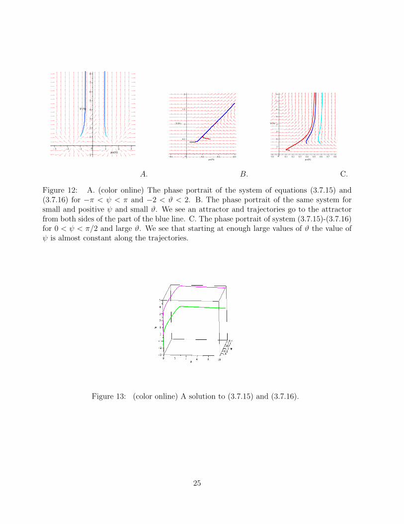
The phase portrait of the system of eqs. (3.7.15) and (3.7.16) is presented in Fig.12. The 3dplot of ψ and ϑ as functions of N found by numerical solution of the system of eqs. (3.7.15)and (3.7.16) is presented in Fig.13.

In Fig.12.A and 12.C we see that ψ is almost constant for large ϑ, i.e. for ϑ(N) > ϑ0 =ϑ(N0) we have ψ(N) ≈ ψ(N0).

3.7.4 Critical points

We can see in the phase portrait Fig.12 that there are the critical points. They solve theequations

3

2sin2 ψ0 sinh 2ϑ0 +

1

2bsin 2ψ0 coshϑ0 = 0, (3.7.17)

1

bcos2 ψ0 sinhϑ0 −

3

2sin 2ψ0 = 0. (3.7.18)

There are only the following real solutions to the system of equations (3.7.17) and (3.7.18)

ψ0 = ±π2, ϑ0 = 0; (3.7.19)

ψ0 = 0, ϑ0 = 0; (3.7.20)

ψ0 = π, ϑ0 = 0. (3.7.21)

24

A. B. C.

Figure 12: A. (color online) The phase portrait of the system of equations (3.7.15) and(3.7.16) for −π < ψ < π and −2 < ϑ < 2. B. The phase portrait of the same system forsmall and positive ψ and small ϑ. We see an attractor and trajectories go to the attractorfrom both sides of the part of the blue line. C. The phase portrait of system (3.7.15)-(3.7.16)for 0 < ψ < π/2 and large ϑ. We see that starting at enough large values of ϑ the value ofψ is almost constant along the trajectories.

Figure 13: (color online) A solution to (3.7.15) and (3.7.16).

25

3.7.5 Near critical points

Let us examine the system near critical points ψ0 = ±π2, ϑ0 = 0. Let us take, for example,

ψ ≈ π2−∆ψ, ϑ ≈ ∆ϑ and linearize (3.7.15) and (3.7.16). We get

∆ϑ′ = 3∆ϑ+1

b∆ψ, (3.7.22)

∆ψ′ = 3∆ψ. (3.7.23)

Solutions to (3.7.22) and (3.7.23) are given by

∆ϑ =1

2(C2N + 2C1b)e

3N , (3.7.24)

∆ψ = C2b

2e3N . (3.7.25)

Let us write φ, φ and H near this point. Taking into account (3.7.11)-(3.7.14) we get

φ′ ≈√

2

l+O(∆ψ2), (3.7.26)

φ ≈√

2Λ

(2

C2be3N− b

6C2e

3N

), (3.7.27)

φ ≈√

2 b

l

(1

2(C2N + 2C1b)e

3N

)(2

C2be3N+

b

12C2e

3N

), (3.7.28)

H ≈ bµ

(2

C2be3N+

b

12C2e

3N

)(1− 1

2

(1

2(C2N + 2C1b)e

3N

)2). (3.7.29)

3.7.6 Solution for the large ϑ limit

Let us keep in (3.7.15) and (3.7.16) only the terms that dominate in the large ϑ region. Wehave

ϑ′ =3

4sin2 ψ e2ϑ, (3.7.30)

ψ′ =1

2bcos2 ψeϑ. (3.7.31)

In Fig.14 we can compare the phase portraits for the system of equations (3.7.15) and (3.7.16)with that of equations (3.7.30) and (3.7.31). From these plots we see that for the large ϑlimit the approximation (3.7.30), (3.7.31) works rather well and for small it does not worksat all.

From (3.7.30) and (3.7.31) we have

dϑ

eϑ=

3b

2

sin2 ψ

cos2 ψdψ.

That gives

e−ϑ =3b

2(ψ − tanψ) + C, (3.7.32)

26

Figure 14: (color online) The comparison of the exact solution to (3.7.15), (3.7.16) (thinklines) with the approximate solution (thick dotted lines).

where

C ≡ 3b

2(tanψ0 − ψ0) + e−ϑ0 .

Let us now substitute (3.7.32) into (3.7.31). We get

ψ′ =1

2b

cos2 ψ3b2

(ψ − tanψ) + C. (3.7.33)

We see that due to possible zeros of the denominator in the RHS of (3.7.33) singular pointscan appear. Since ψ − tanψ is negative, a positive C leads to a singularity.

For us it is important that N increases during the dynamics (this corresponds to expan-sion), meanwhile ψ can increase or decrease, this does not matter. We can say, that if theRHS of (3.7.33) is positive, then ψ increases with increasing N , or if the RHS of (3.7.33)is negative, then ψ decreases with increasing N . In the case of a singularity, before thesingularity ψ increases, and after ψ decreases, see Fig.15.

We can solve (3.7.33) explicitly to get an implicit form of a dependence of ψ on N

Υ(ψ,C, b)−Υ(ψ0, C, b) = N −N0, (3.7.34)

where

Υ(ψ,C, b) ≡ 3 b2ψ tanψ + 3 b2 ln (cosψ)− 3b2

2 (cosψ)2 + 2Cb tanψ.

27

Figure 15: (color on line) 2d plot of the RHS of (3.7.33) for b = 2 and 0 < ψ < π/2and different values of C: C=1 (green pointed line), C=-5 (grey dashed line), C=5 (bluedashed-pointed line) and C=0 (magenta solid line).

From Fig.16 we see that for positive values of C there are maximal values of Υ(ψ,C, b).These maxima are reached at some point 0 < ψmax < π/2, that satisfies the relation

3b(ψmax − tanψmax) + 2C = 0 ⇒ tanψmax − ψmax =2C

3b. (3.7.35)

If ψmax is close to zero, we can expand the LHS of the second formula in (3.7.35) in theTaylor expansion and get ψmax ≈ (2C

b)1/3. This obviously works for 2C

b< 1.

For negative values of C the maxima are at ψmax = 0 and these solutions correspond todecreasing N for increasing ψ.

Let us now examine what this approximation gives for the variables φ, φ. In the accepted

28

A. B.

Figure 16: (color online) A. 2d plot of Υ(ψ,C, b) for different values of C and b = 2 (thesolid aquamarine thick line corresponds to C = 5, the solid think line corresponds to C = 2,the dashed thick line corresponds to C = −5, the solid blue line corresponds to C = 0). B.2d plot of Υ(ψ,C, b) for C = 0 and b = 2.

approximation (3.7.11)-(3.7.14) gives

φ′ = ≈√

2

2lsinψeϑ, (3.7.36)

φ =√

2Λ tanψ, (3.7.37)

φ ≈√

2Λ

µ

1

cosψ, (3.7.38)

H ≈ 2l√

Λ

cosψe−ϑ. (3.7.39)

Note that instead of the Friedmann equation we have

8πG

3

µ2

2φ2 − 8πG

3

1

2φ2 ≈ 8πG

3Λ. (3.7.40)

From formulae (3.7.37), (3.7.38) we see that increasing ψ within (0 < ψ < π/2) corre-sponds to increasing φ and φ. From the phase portrait Fig.3 we see that for increasing timekeeping on the part of the solution corresponding to H > 0 (but very small) we increase φand φ. From this consideration we conclude that to know the behavior near the “separatrix”with positive H we can take the regime near ψmax from the left. We can also say that thefield and its time derivative reach the values

φboundary =

√2Λ

µ

1

cosψmax, (3.7.41)

φboundary =√

2Λ tanψmax, (3.7.42)

(that belongs to the boundary of the forbidden region) and then dynamics becomes con-tracting.

29

So, we have the following picture: We start from some N0 and some ψ0. Suppose thatwe take a suitable ϑ0 (let us remind that we assume that ϑ0 is large enough) to guaranteethat

• C > 0. Since we study dynamics with H > 0, i.e. the number of foldings shouldincrease, N0 < Nmax(C). In this case we have increasing N during the time evolutiontill N reaches Nmax(C). Nmax can be found from (3.7.34)

Nmax = Υ(ψmax, C, b)−Υ(ψ0, C, b) +N0. (3.7.43)

• C = 0. In this case the number of foldings decreases with increasing ψ, and as we haveseen before, increasing ψ corresponds to increasing φ.

• C < 0, here we have also a decreasing number of e-foldings.

We can estimate the dynamics near ψ = ψmax. For this purpose let us expand Υ nearψ = ψmax. We have

Υ(ψ,C, b) = Υ(ψmax, C, b) (3.7.44)

+3b

2

tanψmaxcos2 ψmax

(2 bψmax +

4

3C − 3 b tanψmax

)(ψ − ψmax)2 +O((ψ − ψmax)3)

From the condition that we are near the maximum and 0 < ψmax < π/2 it follows that

2 bψmax +4

3C − 3 b tanψmax = −b tanψmax < 0

Now eq. (3.7.34) takes the form

υ(ψ − ψmax)2 ≈ −Υ(ψ0, C, b) + Υ(ψmax, C, b)−N +N0, (3.7.45)

where

υ ≡ −1

2

tanψmaxcos2 ψmax

(6 b2ψmax + 4 bC − 9 b2 tanψmax

)> 0

and we get

ψ = ψmax −1

υ1/2

√Υ(ψmax, C, b)−Υ(ψ0, C, b)−N +N0. (3.7.46)

As ψmax and C are functions of the initial data denoting

N0 ≡ Υ(ψmax, C, b)−Υ(ψ0, C, b) +N0,

we can rewrite (3.7.46) as

ψ(N) = ψmax −1

υ1/2

√N0 −N. (3.7.47)

Let’s now find the dependence on the time. Due to (3.7.39) and (3.7.32) we have

dt

dN≈ 1

2l√

Λ

cosψ3b2

(ψ − tanψ) + C.

30

Substituting here the explicit dependence of ψ on N , eq. (3.7.47), we get

t− t0 ≈∫ N

N0

dN

2l√

Λ

cosψ(N)3b2

(ψ(N)− tanψ(N)) + C,

where ψ(N) is given by (3.7.47). Making the change of variables

u ≡ 1

υ1/2

√N0 −N,

we get

t− t0 ≈ −∫ √

N0−Nυ1/2

√N0−N0

υ1/2

uvdu

l√

Λ

cos(ψmax − u)3b2

(ψmax − u− tan(ψmax − u)) + C.

Expanding the integrand near ψmax up to u we get

t− t0 ≈1

l√

Λ√

32

tanψmax

(√N0 −N0 −

√N0 −N)

+1

l√

Λ

(sinψmax cosψmax − 1)

3b sin3 ψmaxcos2 ψmax(N −N0).

(3.7.48)

Let’s keep only the leading term (linear in u). Then equation (3.7.48) can be rewritten as

t ≈ t0 − ν√N0 −N, N0 −N ≈

(t− t0)2

ν2, (3.7.49)

where ν is the function of the initial data and has the form

ν =1

l√

Λ√

32

tanψmax

.

Substituting this expression into the asymptotic for φ near φboundary given by (3.7.41) we get

φ(t) ≈√

2Λ

µ

1

cos(ψmax − t0−tυ1/2ν

). (3.7.50)

4 Stretched Higgs in FRW

4.1 Stretched coupling constant

In this section we consider the case of non-positively defined Higgs potential. As it wasmentioned in Introduction due to non-locality of the fundamental theory the effective stretchof a coupling constant occurs. We will write the equation of evolution in the following form

eα2eff

(φ+ 3H φ− µ2φ

)= −εφ3, (4.1.1)

H2 =8πG

3

(eα

2eff

2( φ2 − µ2φ2) +

1

4εφ4 + Λ

). (4.1.2)

31

Therefore, we have the ordinary theory with redefined constants

φ+ 3H φ− µ2φ = −εeffφ3, (4.1.3)

H2 =8πGeff

3

(1

2φ2 − 1

2µ2φ2 +

εeff4

φ4 + Λeff

), (4.1.4)

where

Geff = Geα2eff , (4.1.5)

εeff = εe−α2eff , (4.1.6)

Λeff = Λe−α2eff . (4.1.7)

We have alsoH = −4πGeff φ

2. (4.1.8)

4.2 Phase portraits for different Λeff

In this subsection we consider the phase portraits for the Higgs field for different values ofthe total cosmological constant. The Friedmann equation has the form (here and below wewrite G, ε instead Geff and εeff )

H2 =8πG

3

(1

2φ2 +

ε

4(φ2 − a2)2 + Λ

), (4.2.9)

where

Λ = Λeff −εa4

4.

We will consider the cases Λ > 0, Λ = 0 and Λ < 0. As we just mentioned the unusual caseΛ < 0 appears due to the effect of the stretch of coupling constant in nonlocal theory.

4.2.1 The case of Higgs potential without extra cosmological constant, Λeff = εa4

4

In this case we deal with the potential presented in Fig.17.A. and the phase portrait doesn’thave a forbidden domain. This case has been considered in many works and we discuss it inSect.2.

4.2.2 Λeff = 0

In the case Λeff = 0, see Fig.17.B., the phase portrait does have the forbidden region andthe reheating domain is totally or partially removed (dependently on the trajectory). Thecharacteristic feature of this case is an appearance of the contraction regime. To see thislet’s consider this case in more details.

32

A. B. C.

Figure 17: A. The potential in the case Λeff = εa4

4. B. The potential in the case Λeff = 0.

C. The potential in the case 0 < Λeff <εa4

4.

φ

φ

A.

φ

φ

B.

Figure 18: (color online) A. The phase portraits of equation (4.2.10). The forbidden regionconsists of two merged holes. Colored line presents the trajectory starting from some pointof the phase diagram. The trajectory reaches the border of the forbidden area. B. Thephase portrait of equation (4.2.11). Colored line presents trajectory that is continuation ofthe trajectory presented in the left panel. It is a solution to the Friedman equation withnegative values of H.

Our goal is to see the future and the past singularities of the Higgs scalar field in theFRW metric. EOM describing inflation is

φ+ 3

√8πG

3

(1

2φ2 − µ2

2φ2 +

ε

4φ4

)φ = +µ2φ− εφ3. (4.2.10)

The phase portrait of this system is presented in Fig.18.A. The contraction phase satisfies

33

equation

φ− 3

√8πG

3

(1

2φ2 − µ2

2φ2 +

ε

4φ4

)φ = +µ2φ− εφ3 (4.2.11)

and its phase portrait is presented in Fig.18.B. To study the infinite phase space following [51]let us use dimensionless variables (X, Y, Z) (3.3.2)-(3.3.4). In these variables the dynamicalsystem has the form

Xτ = Y, (4.2.12)

Yτ = X − 3ZY − gX3, (4.2.13)

Zτ = −X2 − 2Y 2 − Z2 +g

2X4, (4.2.14)

where g = ε34

m2p

πµ2.

The integral of motion is

−X2 + Y 2 − Z2 +g

2X4.

To describe Λeff = 0 we take

−X2 + Y 2 − Z2 +g

2X4 = 0. (4.2.15)

The Friedmann equation keeps the dynamics of the system on the surface (4.2.15). Thissurface has two parts: one corresponds to expansion (H > 0) and the second one correspondsto contraction.

The phase portrait of the dynamical system (4.2.12)-(4.2.14) is presented in Fig.18.To study the infinite phase space we use the spherical coordinates (ρ, θ, ψ) (3.3.9)-(3.3.11),

see Section 3. In these coordinates EOM have the form

ρσ = ρ(1− ρ)2

[sin 2ψ sin2 θ − ρ

1− ρcos θ(1 + 4 sin2 ψ sin2 θ)

− g ρ2

(1− ρ)2cos3 ψ sin3 θ

(sinψ sin θ − 1

2sin 2θ cosψ

)](4.2.16)

ψσ = −3

2ρ sin 2ψ cos θ + (1− ρ) cos 2ψ − g ρ2

1− ρsin2 θ cos4 ψ (4.2.17)

θσ =1

2(1− ρ) sin 2ψ sin 2θ + ρ sin θ(1 + sin2 ψ − 4 sin2 ψ cos2 θ)

−g2

ρ5

(1− ρ)4sin5 θ cos4 ψ (4.2.18)

The phase portrait of this system of equations is presented in Fig.19. We see thattrajectories are symmetric under the reflection with respect to the boundary of the forbiddenarea. We also see the two singular points – at the past (cosmological singularity) and thesame in the future.

34

s

FS

PS

s

A.

FS

PS

B.

Figure 19: (color online) A. The phase portrait of equations (4.2.16) – (4.2.18) in the (ρ, θ)-plane. The black thin line corresponds to θ = ±π/2. Blue parts of lines represent contractionand red parts represent expansion. We see the symmetry with respect to replacing the redparts by the blue parts of lines. FS and PS are future and past cosmological singularities.B. The 3-dimensional plot in (ρ, θ, ψ) coordinates of the same phase portrait.

4.2.3 0 < Λeff <εa4

4

In this case the potential is presented in Fig.17.C., the forbidden domain contains two non-connected parts.

Near the top of the potential the Higgs potential can be approximated with the tachyonpotential

V (φ) ≈ −εa2

2φ2 + Λeff . (4.2.19)

We can note that near the top of the hill the slow-roll conditions can be satisfied andthe scenario of “new inflation” is possible. To illustrate this we present the plot for slow-rollparameters ε and |η| depending on the value of φ in Fig.20 A and B. As we see near the topthe tachyon approximation can represent the exact model.

To get some estimation in the region near the top one can use the same technique as inthe Section 3.

5 Conclusion

To conclude, let us remind that our logic was the following. We started from nonlocality.Using the “stretched” arguments presented by [25, 26] we have got non-positive definedpotential. There exist a region where we can use the tachyon approximation. For freetachyon there are 4 eras of evolution: i) from the past cosmological singularity to reaching

35

A. B.

Figure 20: (color online) A. The slow-roll parameter ε depending on the value of φ. The solidline represents the plot in the case of the exact Higgs potential, the dashed line representsthe plot in the case of the tachyon approximation. B. The slow-roll parameter |η| dependingon the value of φ. The solid line represents the plot in the case of the exact Higgs potential,the dashed line represents the plot in the case of the tachyon approximation.

the hill, ii) rolling from the hill, iii) transition from expansion to contraction, iv) contractionto the future cosmological singularity.

For the Higgs model with an extra negative cosmological constant and small couplingconstant produces 5 eras of evolution: i) the ultra-hard regime starting from the past cos-mological singularity, ii) reaching the hill (here we can use the free tachyon approximation),iii) rolling from the hill (here we can use the free tachyon approximation), iv) the transitionfrom expansion to contraction (here we can use the free tachyon approximation),v) contraction to the future cosmological singularity.

Let us note that there are the following differences between dynamics for positivelydefined and non-positively defined potentials in the FRW cosmology. For non-positivelydefined potential there is a stage of transition from expansion to contraction and there is nothe oscillation regime ending with the zero field configuration. To obtain the era of reheatingfor the Higgs potential with an extra negative cosmological constant one can introduce anextra matter interacting with the Higgs field.

Acknowledgements

We would like to thank I.V. Volovich and S.Yu. Vernov for the helpful discussions. Thework is partially supported by grants RFFI 11-01-00894-a and NS – 4612.2012.1

36

References

[1] A. Linde, Inflation and Quantum cosmology, Academic Press, Boston, 1990.

[2] V.F. Mukhanov, Physical Foundations of Cosmology, Cambridge University Press,2005.

[3] S. Weinberg, Gravity and Cosmology, Oxford Univ.Press, 2008.

[4] D.S. Gorbunov and V.A. Rubakov, Introduction to the Theory of the Early Universe,URSS, Moscow, 2009 (in Russian).

[5] A.A. Starobinsky, Phys. Lett. B 91, 99 (1980);A.H. Guth, Phys. Rev. D 23, 347 (1981);A.D. Linde, Phys. Lett. B 108, 389 (1982);A. Albrecht and P.J. Steinhardt, Phys. Rev. Lett. 48, 1220 (1982)

[6] A.D. Linde, “Chaotic Inflation,” Phys. Lett. B 129, 177 (1983).

[7] A.D. Linde, “Initial Conditions For Inflation,” Phys. Lett. B 162 (1985) 281.

[8] V.F. Mukhanov, H.A. Feldman and R.H. Brandenberger, Theory of cosmological per-turbations, Phys. Rept. 215 (1992) 203–333

[9] F.L. Bezrukov and M. Shaposhnikov, “The Standard Model Higgs boson as the infla-ton,” Phys. Lett. B659 (2008) 703, arXiv:0710.3755,

[10] J. Garcia-Bellido, D.G. Figueroa, and J. Rubio, “Preheating in the StandardModel with the Higgs-Inflaton coupled to gravity,” Phys. Rev. D79 (2009) 063531,arXiv:0812.4624

[11] A. De Simone, M.P. Hertzberg, and F. Wilczek, “Running In ation in the StandardModel,” Phys. Lett. B678 (2009) 1, arXiv:0812.4946

[12] A.O. Barvinsky, A.Y. Kamenshchik, C. Kiefer, A.A. Starobinsky, and C.F. Steinwachs,“Higgs boson, renormalization group, and cosmology,” arXiv:0910.1041

[13] J.L.F. Barbon and J.R. Espinosa, “On the Naturalness of Higgs Inflation”, Phys. Rev.D79 (2009) 081302, arXiv:0903.0355

[14] F. Bezrukov, A. Magnin, M. Shaposhnikov and S. Sibiryakov, “Higgs inflation: con-sistency and generalisations,” JHEP 1101 (2011) 016,arXiv:1008.5157

[15] E. Babichev, V. Mukhanov, A. Vikman “k-Essence, superluminal propagation, causal-ity and emergent geometry.” JHEP 0802:101,2008, arXiv:0708.0561

[16] N. Arkani-Hamed, H.-C. Cheng, M.A. Luty and S. Mukohyama, “Ghost condensa-tion and a consistent infrared modification of gravity,” JHEP 0405 (2004) 074 hep-th/0312099

37

[17] I.Ya. Aref’eva, Nonlocal String Tachyon as a Model for Cosmological Dark Energy,2006 AIP Conf. Proc. 826, pp. 301–311, astro-ph/0410443

[18] I.Ya. Aref’eva and L.V. Joukovskaya, 2005 Time lumps in nonlocal stringy models andcosmological applications, JHEP 0510, 087, hep-th/0504200

[19] G. Calcagni, Cosmological tachyon from cubic string field theory, JHEP 0605, 012(2006), hep-th/0512259

[20] I.Ya. Aref’eva, A.S. Koshelev, Cosmic acceleration and crossing of w = −1 barrier innon-local Cubic Superstring Field Theory model, JHEP 0702:041, 2007, hep-th/0605085

[21] N. Barnaby, T. Biswas and J.M. Cline, “p-adic Inflation,” JHEP 0704 (2007) 056hep-th/0612230

[22] I.Ya. Aref’eva and I.V. Volovich, “On the null energy condition and cosmology,” Theor.Math. Phys. 155, 503 (2008), hep-th/0612098.

[23] A.S. Koshelev, “Non-local SFT Tachyon and Cosmology,” JHEP 0704 (2007) 029hep-th/0701103

[24] I.Ya. Aref’eva, L.V. Joukovskaya, and S.Yu. Vernov, Bouncing and accelerating solu-tions in nonlocal stringy models JHEP 0707 (2007) 087, hep-th/0701184

[25] J.E. Lidsey, Stretching the inflaton potential with kinetic energy, Phys. Rev. D76,043511 (2007), hep-th/0703007.

[26] N. Barnaby and J.M. Cline, “Large Nongaussianity from Nonlocal Inflation,” JCAP0707 (2007) 017 arXiv:0704.3426

[27] G. Calcagni, M. Montobbio and G. Nardelli, “Route to nonlocal cosmology,” Phys.Rev. D 76, 126001 (2007) arXiv:0705.3043

[28] L. Joukovskaya, Dynamics in Nonlocal Cosmological Models Derived from String FieldTheory, Phys. Rev. D 76, 105007 (2007), arXiv:0707.1545

[29] I.Ya. Aref’eva, L.V. Joukovskaya, and S.Yu. Vernov, Dynamics in nonlocal linear mod-els in the Friedmann–Robertson–Walker metric, J. Phys. A: Math. Theor. 41 (2008)304003, arXiv:0711.1364

[30] N. Barnaby and J.M. Cline, “Predictions for Nongaussianity from Nonlocal Inflation,”JCAP 0806 (2008) 030 arXiv:0802.3218

[31] I.Ya. Aref’eva and A.S. Koshelev, “Cosmological Signature of Tachyon Condensation,”JHEP 0809 (2008) 068 arXiv:0804.3570

[32] D.J. Mulryne and N.J. Nunes, “Difusing nonlocal infation: Solving the feld equationsas an initial value problem,” Phys. Rev. D 78 (2008) 063519 arXiv:0805.0449

38

[33] L.V. Joukovskaya, “Dynamics with Infinitely Many Time Derivatives in Friedmann-Robertson-Walker Background and Rolling Tachyon,” JHEP 0902 (2009) 045arXiv:0807.2065

[34] D.J. Mulryne and N.J. Nunes, Non-linear non-local Cosmology, AIP Conf. Proc. 1115(2009) 329–334, arXiv:0810.5471

[35] N. Barnaby, Nonlocal Inflation, Can. J. Phys. 87 (2009) 189–194, arXiv:0811.0814

[36] S.Yu. Vernov, Localization of nonlocal cosmological models with quadratic potentials inthe case of double roots, Class. Quant. Grav. 27 (2010) 035006, arXiv:0907.0468;

[37] A.S. Koshelev and S.Yu. Vernov, Analysis of scalar perturbations in cosmological mod-els with a non-local scalar field, Class. Quant. Grav. 28 (2011) 085019, arXiv:1009.0746

[38] F. Galli, A.S. Koshelev, Multi-scalar field cosmology from SFT: an exactly solvableapproximation, Theor. Math. Phys. (2010) 164, 1169–1175 Teor. Mat. Fiz. 164 (2010)401–409, arXiv:1010.1773

[39] I.Ya. Arefeva, D.M. Belov, A.A. Giryavets, A.S. Koshelev and P.B. Medvedev, “Non-commutative field theories and (super)string field theories,” hep-th/0111208.

[40] L. Boubekeur and D. H. Lyth, “Hilltop inflation,” JCAP 0507 (2005) 010 hep-ph/0502047

[41] G.N. Felder, A.V. Frolov, L. Kofman and A.D. Linde, “Cosmology with negative po-tentials,” Phys. Rev. D 66 (2002) 023507 hep-th/0202017

[42] K. Tzirakis, W.H. Kinney, “Inflation over the hill,” Phys. Rev. D75, 123510 (2007),astro-ph/0701432.

[43] I.Ya. Aref’eva, A.S. Koshelev, D.M. Belov and P.B. Medvedev, “Tachyon condensationin cubic superstring field theory,” Nucl. Phys. B 638, 3 (2002) hep-th/0011117

[44] A. Sen, “Stable nonBPS bound states of BPS D-branes,” JHEP 9808, 010 (1998)hep-th/9805019

[45] V.S. Vladimirov and Ya.I. Volovich, “On the nonlinear dynamical equation in thep-adic string theory,” Theor. Math. Phys. 138 (2004) 297, math-ph/0306018.

[46] Ya. Volovich, “Numerical study of nonlinear equations with infinite number of deriva-tives,” J. Phys. A A 36, 8685 (2003) math-ph/0301028

[47] N. Moeller and B. Zwiebach, “Dynamics with infinitely many time derivatives androlling tachyons,” JHEP 0210 (2002) 034 hep-th/0207107

[48] H. Yang, Stress tensors in p-adic string theory and truncated OSFT, JHEP 0211 (2002)007, hep-th/0209197

39

[49] I.Ya. Aref’eva, L.V. Joukovskaya, and A.S. Koshelev, Time evolution in superstringfield theory on nonBPS brane. 1. Rolling tachyon and energy momentum conservation,JHEP 0309 (2003) 012, hep-th/0301137

[50] I.Ya. Aref’eva and I.V. Volovich, “Cosmological Daemon,” JHEP 1108 (2011) 102,arXiv:1103.0273.

[51] V.A. Belinsky, I.M. Khalatnikov, L.P. Grishchuk and Ya.B. Zeldovich, Phys.Lett. B155 (1985) 232

[52] L.A. Urena-Lopez and M.J. Reyes-Ibarra, “On the dynamics of a quadratic scalar fieldpotential,” Int. J. Mod. Phys. D 18 (2009) 621 arXiv:0709.3996

[53] A.R. Liddle, P. Parsons and J.D. Barrow, “Formalizing the slow roll approximation ininflation,” Phys. Rev. D 50, 7222 (1994), astro-ph/9408015.

[54] E.J. Copeland, A.R. Liddle, D. Wands, “Exponential potentials and cosmological scal-ing solutions,” Phys. Rev. D57, 4686-4690 (1998), gr-qc/9711068 .

[55] A. de la Macorra, G. Piccinelli, “General scalar fields as quintessence,” Phys. Rev.D61, 123503 (2000), hep-ph/9909459.

[56] D. Boyanovsky, C. Destri, H.J. De Vega and N.G. Sanchez, “The Effective Theory ofInflation in the Standard Model of the Universe and the CMB+LSS data analysis,”Int. J. Mod. Phys. A 24 (2009) 3669, arXiv:0901.0549

40