NBER WORKING PAPER SERIES

FUEL ECONOMY AND SAFETY:THE INFLUENCES OF VEHICLE CLASS AND DRIVER BEHAVIOR

Mark R. Jacobsen

Working Paper 18012http://www.nber.org/papers/w18012

NATIONAL BUREAU OF ECONOMIC RESEARCH1050 Massachusetts Avenue

Cambridge, MA 02138April 2012

The University of California Energy Institute has generously provided funding in support of this work.I thank seminar participants at Harvard University, The University of Maryland, Columbia University,the UC Energy Institute, the American Economic Association Annual Conference, and the NBERSummer Institute for their helpful suggestions. The views expressed herein are those of the authorand do not necessarily reflect the views of the National Bureau of Economic Research.

NBER working papers are circulated for discussion and comment purposes. They have not been peer-reviewed or been subject to the review by the NBER Board of Directors that accompanies officialNBER publications.

© 2012 by Mark R. Jacobsen. All rights reserved. Short sections of text, not to exceed two paragraphs,may be quoted without explicit permission provided that full credit, including © notice, is given tothe source.

Fuel Economy and Safety: The Influences of Vehicle Class and Driver BehaviorMark R. JacobsenNBER Working Paper No. 18012April 2012JEL No. L9,Q4,Q5

ABSTRACT

Fuel economy standards change the composition of the vehicle fleet, potentially influencing accidentsafety. I introduce a model of the fleet that captures risks across interactions between vehicle typeswhile simultaneously recovering estimates of unobserved driving safety behavior. The model importantlyincludes the ability to consider the selection of driver types across vehicles. I apply the model to thepresent structure of U.S. fuel economy standards and find an adverse effect on safety: Each MPG incrementto the standard results in an additional 149 fatalities per year in expectation. I next show how twoalternative regulatory provisions, including one slated to enter effect next year, can fully offset thenegative safety consequences; minor changes in the regulation produce a robust, near-zero changein accident fatalities while conserving the same quantity of gasoline.

Mark R. JacobsenDepartment of Economics, 0508University of California, San Diego9500 Gilman DriveLa Jolla, CA 92093and NBERm3jacobs@ucsd.edu

2

1. Introduction

Fuel economy standards create an incentive for manufacturers to alter the

composition of the vehicle fleet toward smaller and lighter vehicles, potentially changing

overall accident safety. The direction and magnitude of the effect depends on the set of

interactions between all vehicles in the fleet: larger vehicles tend to offer their own

occupants greater safety, but do so at considerable expected cost to the drivers of smaller

cars. I show how the effects of vehicle safety can dramatically change the cost-benefit

calculus for new fuel economy rules phasing in through 2016.1 The need to understand the

size and direction of the relation between fuel economy and safety is further underscored by

the announcement of even stronger policy through 2025, nearly doubling the current fuel

economy requirement.2

There is a long related literature on vehicle engineering and safety, much of it

focusing on specific physical characteristics of vehicles like weight or the inclusion of new

safety technologies. Kahane (2003) and the National Research Council (2002) provide

summaries. Evans (2001) and Anderson and Auffhammer (2011) parameterize the effect of

weight in particular and make a careful effort to control for driver selection. In general this

literature finds that heavier vehicles offer additional protection in accidents, but in cases

where two vehicles are involved the extra weight imposes risk on the other driver. The

National Research Council (2002) applies one such simple relationship between overall

vehicle safety and weight and suggests that 2,000 additional deaths annually could be

associated with existing fuel economy standards.3

There is also a recent literature that investigates the danger that light trucks

specifically (a category including pickups, minivans, and SUV's) pose when they are

involved in an accident with a sedan. White (2004) shows that the protective effect of light

trucks for their own drivers combines with severe external risks to create an arm's race in

1 Environmental Protection Agency and Department of Transportation (2010). There were 37,261 U.S. traffic fatalities in 2008. 2 The White House Office of the Press Secretary (2011). 3 See Portney et al (2003) and Crandall and Graham (1989) for further discussion.

3

vehicle choice. Gayer (2004) examines the safety of light trucks using snowfall as an

instrument to predict their frequency in the fleet. He shows that there is a significantly

higher overall fatality risk in areas with a greater number of light trucks, suggesting that fuel

economy incentives – if they acted to discourage pickups and SUV's – might in fact have the

opposite effect, improving safety outcomes.

The first main contribution of this paper is an econometric model that flexibly nests

both strands of the literature. My model provides what I believe is the first approach to

consider safety in counterfactual fleets where characteristics like weight can change

simultaneously with composition across vehicle classes. A key challenge is to model driver

selection into vehicle types, observing that drivers will re-optimize over their choice of

vehicle as fuel economy policy changes the composition of the fleet. My estimation

technique introduces a semi-parametric method to measure this effect of unobserved driver

behavior: in policy counterfactuals I show that the ability to capture driver behavior is

pivotal to the policy results, changing the sign of the estimated welfare impacts.

My estimation approach begins with a system of equations describing single-vehicle

and two-vehicle accident fatality rates, all expressed per mile driven. In order to abstract

from weight or the light truck definition in isolation I bin vehicles into classes (ten in the

dataset I employ) spanning the wide variety of sizes, weights, and shapes in the fleet. The

model allows estimates of the internal and external safety costs when vehicles in each bin

interact with every other.4 Restrictions across the equations allow me to empirically

separate unobserved driver risk behavior from underlying vehicle safety.

The second contribution here, before moving to the policy question on fuel economy

standards, lies in the empirical estimates themselves. I use U.S. accident data to estimate a

matrix of risks across 110 specific accident types, all estimated without parameterizing

vehicle characteristics.5 When cutting this matrix along the dimension of weight I am able

4 The estimates are semi-parametric in this sense since no restrictions are placed on the combination of physical characteristics in a bin. Among other dimensions classes differ by weight, wheelbase, engine size, fuel economy, and passenger capacity. 5 There are 100 types of two-car accidents, corresponding to all interactions of vehicles across bins, and 10 types of single car accidents.

4

to show that my empirical results are consistent with the earlier literature examining weight

in isolation. If I instead divide my estimates according to class, light truck or sedan, I

further find the results are consistent with the literature looking at the dangers imposed by

light trucks. Finally, and in contrast to either of these earlier approaches, the matrix of

estimates also captures safety interactions along all other physical dimensions where vehicle

bins differ.

My empirical results also contain a novel measure of the residual riskiness of drivers

who select into different types of vehicles, expressed up to a constant. Since I can allow all

components of driver risk to remain unobserved these estimates capture, for example, a

tendency to drive drunk,6 the safety of roads in the driver's geographical area, and Peltzman-

type effects where the protective nature of a vehicle itself may affect driving behavior.

Finally, a third key contribution of this work returns to the motivating question,

applying my empirical model of the vehicle fleet to consider the safety impacts of fuel

economy policy. I consider three policy variants, all based on current or proposed fuel

economy rules. The estimated safety impacts of the first policy, based on the historical

Corporate Average Fuel Economy (CAFE) rules, depend pivotally on my ability to model

driver behavior: 149 additional annual fatalities are predicted per mile-per-gallon increment.

I next consider a "unified" standard that encourages smaller vehicles overall, now reducing

both weight and the number of light trucks. Unlike earlier studies, I can estimate the degree

to which these factors offset. The increase in fatalities under the unified rule is only 8 per

year, with a zero change included in the confidence band. Finally, I consider a “footprint”

type rule similar to the provisions in fuel economy standards set through 2016. It too has a

near zero impact on safety. I explore robustness of these results to a variety of factors

including Peltzman-type selection effects, weather, age of vehicles, driver versus passenger

fatalities, and the potential frailty of older drivers in accidents.

I limit the policy analysis to the example of fuel economy rules, but since the model

presented here allows consideration of arbitrary counterfactual fleets it could also be applied 6 Levitt and Porter (2001) provide an innovative method to estimate drunk driving rates using innocent vehicles in accidents as control, but in most cases (including the present study) such personal characteristics are difficult to observe.

5

to a number of other questions. For example, the U.S. "cash-for-clunkers" program as

described in Knittel (2009) or the incentives to switch among new and used vehicles in

Busse, Knittel, and Zettelmeyer (2011) may produce changes in safety that importantly alter

the economic efficiency of policy. The definition of vehicle bins is flexible such that

expansions or redefinitions of the vehicle set would allow future investigation of the variety

of policies aiming at influencing composition of the vehicle fleet.

The rest of the paper is organized as follows: Section 2 describes U.S. fuel economy

policy and the role of safety. Section 3 presents the model. Sections 4 and 5 respectively

describe the data and empirical results. Section 6 presents the policy experiments,

combining my empirical results with a model of fuel economy regulation. Section 7

considers three alternative specifications and addresses robustness.

2. Safety and Fuel Economy Regulation

The importance of automobile safety is evident simply from the scale of injuries and

fatalities each year. In 2008 there were 37,261 fatalities in car accidents on U.S. roads and

more than 2.3 million people injured.7 The National Highway Traffic Safety Administration

(NHTSA) is tasked with monitoring and mitigating these risks and oversees numerous

federal regulations that include both automobiles and the design of roads and signals.

To motivate the concern about fuel economy standards with respect to safety

consider the very rough estimate provided in NRC (2002): approximately 2,000 of the traffic

fatalities each year are attributed to changes in the composition of the vehicle fleet due to the

CAFE standards. If we further assume that the standards are binding by about 2 miles per

gallon, this translates to a savings of 7.5 billion gallons of gasoline per year. Valuing the

accident risks according to the Department of Transportation’s methodology this implies a

cost of $1.55 per gallon saved through increased fatalities alone.8 This does not consider

7 NHTSA (2009). 8 The Department of Transportation currently incorporates a value of statistical life of $5.8 million in their estimates. This is conservative relative to the $6.9 million used by EPA.

6

injuries, or any of the other distortions associated with fuel economy rules, yet by itself

exceeds many estimates of the externalities arising from the consumption of gasoline.9

Conversely, a finding that accident risks improve with stricter fuel economy

regulation would present an equally strong argument in favor of stringent fuel economy

rules. The magnitude of the implicit costs involved in vehicle safety motivate the

importance of a careful economic analysis, and mean that even small changes in the

anticipated number of fatalities will carry great weight in determining the optimal level of

fuel economy policy. Current regulation

U.S. fuel economy regulation is in transition, with the rule through 2016 now

complete (Environmental Protection Agency and Department of Transportation [2010]),

while regulatory provisions beyond 2016 remain to be determined. I consider three possible

regulatory regimes, each of which produces a unique effect on the composition of the fleet.

The resulting impacts on the frequency of fatal accidents are similarly diverse:

1) The current Corporate Average Fuel Economy (CAFE) rules: Light trucks and cars are

separated into two fleets, which must individually meet average fuel economy targets. No

direct incentive exists for manufacturers to produce more vehicles in one fleet than the other.

Rather, the incentives to change composition occur inside each fleet: selling more small

trucks and fewer large trucks improves the fuel economy and compliance of the truck fleet.

The same is true inside the car fleet. This produces a distinctive pattern of shifts to smaller

vehicles within each fleet, but without substitution between cars and trucks overall.

2) A unified standard: This type of standard was introduced in California as part of

Assembly Bill 1493, and is under consideration federally.10 It regulates all vehicles together

9 See Parry and Small (2005). 10 Strictly speaking the California bill preserves the fleet definition, but allows manufacturers to “trade” compliance obligations between fleets in order to achieve a single average target. The trading between fleets aligns incentives for all vehicles, making the rule act like a single standard.

7

based only on fuel economy. This includes the effects above while simultaneously

encouraging more small vehicles, broadly shifting the fleet away from trucks and SUV’s and

into cars.

3) A “footprint” standard: This type of rule is in place federally for the years 2012 - 2016

and is also presently being debated for the years 2017 through 2020. It assigns target fuel

economies to each size of vehicle (as determined by width and wheelbase), severely limiting

the incentives for any change in fleet composition. As such it increases the technology costs

of meeting a given target, but was required in the hopes of mitigating the costly safety

consequences discussed above.11 3. A Model of Accident Counts

I model the count of fatal accidents between each combination of vehicle classes as a

Poisson random variable. Vehicle classes in the data represent various sizes and types of

cars, trucks, SUV’s and minivans; covering all passenger vehicles in the U.S.

Define Zij as the count of fatal accidents where vehicles of class i and j have collided

and a fatality occurs in the vehicle of class i. The data will be asymmetric, that is Zij ≠ Z ji ,

to the degree that some vehicle classes impose a greater external risk on others. In the

relatively unusual cases where a fatality occurs in both vehicles in an accident then both Zij

and Zji are incremented.

We can write the total count of fatalities in vehicles of class i as:

(fatalities in class i) = Zij

j∈J∑ (3.1)

11 NHTSA (2008b) discusses the rationale for the footprint rule. Technology costs are higher because all improvement must be achieved through technology; the other rules allow some of the improvement to come from technology and some to come via fleet composition.

8

where J represents the set of all vehicle classes. By changing the order of subscripts we can

similarly write the count of fatalities that are imposed on other vehicles by vehicles of class

i:

(fatalities imposed on others by class i) = Z jij∈J∑ (3.2)

Counts of accidents of each type reflect a combination of factors influencing risk and

exposure. I categorize these factors into three multiplicative components, the first two of

which can be separately identified in estimation: 1) The risk coming from the behavior of

drivers in each vehicle class, 2) risk coming from physical vehicle characteristic alone – I

will term this the “engineering” risk, and 3) the number of vehicles in each class present on

the road at any given time and place. The combination of these three elements determines

the number of fatal accidents in each combination of classes: Intuitively the greater the

driver recklessness, engineering risk, or number of vehicles, the more fatal accidents we

should expect.

Define the three components using: α i The riskiness and safety behavior of the drivers of each vehicle class i (i.e. a separate

fixed effect on driver behavior for each class) βij The risk of a fatality in vehicle i when vehicles from class i and class j collide (i.e.

fixed effects for every possible combination of vehicles) nis The number of vehicles of class i that are present at time and place s

I define the measure of driver riskiness such that it multiplies the overall fatality risk.

For example, a value of α i = 2 will correspond to a doubling of risk relative to an average

driver. High values of α i come from a tendency of class i owners to disobey traffic signals,

drive when distracted or drunk, drive recklessly, or take any other action (observable or

unobservable) that increases the risk of a fatal accident.

9

Combining the definition of dangerous driving behavior with the engineering fatality

risk results in:

Probability of a fatal accident in vehicle i | i, j present =α iα jβij (3.3)

The probability of a fatal accident, conditioned on vehicles i and j being present at a

particular time and place, is modeled as the product of the underlying engineering risk in a

collision of that type, βij , and the parameters representing bad driving, α i and α j .

The multiplicative form contains an important implicit restriction: behaviors that

increase risk are assumed to have the same influence in the presence of different classes and

driver types. I argue that this is a reasonable approximation given that most fatal accidents

result from inattention, drunk driving, and signal violations;12 such accidents give drivers

little time to alter behavior based on attributes of the other vehicle or driver.

Finally I add in the effect of the number of vehicles of each class present in time and

place s. If pickup trucks are less common on urban roads, or minivans tend to be parked at

night, there should be differences in the number of accidents involving these vehicles across

time and space. In the estimation below I bin the data according to time-of-day, average

local income, and urban density – factors that appear to significantly influence both the

composition of the fleet and the probability of fatal accidents. In my notation s will

correspond to bins.

The effect of the quantity of vehicles present in bin s on the number fatalities

expected again takes a natural multiplicative form: If there are twice as many cars of a

certain class on the road then we expect twice as many cars of that class to be involved in an

accident: E(Zijs ) = nisnjsα iα jβij (3.4)

For this final step we add a bin s subscript to the counts Zijs , keeping track of fatal accidents

both by vehicle type and by bin.

12 NHTSA (2008a).

10

Given that the α i terms include unobservable driving behaviors it is impossible to

estimate equation (3.4) alone; it can’t be separately determined if a vehicle class is

dangerous in a causal engineering sense or if the drivers who select it just happen to drive

particularly badly.

The method I propose here separates driver behavior from the underlying safety risk

via a second equation describing single-car accidents. I define the count of fatal single-car

accidents in vehicle class i in location s as Yis where:

E(Yis ) = nisα iλsxi (3.5)

The four parameters are: nis (As above) The number of vehicles of class i present in bin s

α i (As above) The riskiness of drivers owning vehicles of class i

λs A bin-specific fixed effect allowing the overall frequency of fatal single-car

accidents to vary freely across time and space.

xi The relative fatality risk to occupants of class i in a standardized collision (to be

measured using government crash tests).

The key restriction across equations (3.4) and (3.5) is that the dangerous behaviors

contained in α i multiply both the risk of single-car accidents and the risk of accidents with

other vehicles. This may be a better assumption for some behaviors (drunk driving,

recklessness) than others (falling asleep) but I will show below that it appears to fit the data

well. Note that the assumption is not that the absolute risk of single and two-car accidents

are always proportional (clearly single car accidents are more frequent at night, for example)

but rather it restricts the way that driver behavior multiplies those risks.

Comparison with other models in the literature

Much of the previous work focusing on the influence of weight of vehicles (see

Kahane [2003]) has taken a parametric approach and attempts to isolate the effect of weight

11

alone. By assigning a complete set of fixed effects for all possible interactions, βij , I can

still recover information about vehicle weight, but add considerable flexibility in form and

am able to account for other attributes that vary by class. The cost to my approach comes in

terms of demands on the data and the degree of aggregation (I will aggregate to 10 distinct

classes, or 100 βij fixed effects).

Wenzel and Ross (2005) describe overall risks using a similarly flexible approach for

vehicle interactions but importantly do not model driving safety behavior, and so are unable

to separate it from underlying engineering risk. For purpose of comparison I provide

estimates of a restricted version of my model where I set all the α i ’s to be equal. The

parameter estimates turn out to be quite different, so much so in fact that the primary policy

implication is reversed in sign. 4. Data

I assemble data on each of the three variables needed to identify the parameters of

(3.4) and (3.5):

• Comprehensive count of fatal accidents, Zijs and Yis

• The number of vehicle miles driven in each class, ni

• Crash test data to describe risks in single-car accidents, xi

Fatal accident counts

The count data on fatal accidents represent the core information needed to estimate

my model. I rely on the comprehensive Fatal Accident Reporting System (FARS), which

records each fatal automobile accident in the United States. The dataset is complete and of

high quality, due in part to the importance of accurate reporting of fatal accidents for use in

legal proceedings. If such complete data were available for accidents involving injuries or

damage to vehicles it could be used in a similar framework to the one I propose, but

reporting bias and a lack of redundancy checking in police reports for minor accidents make

those data less reliable.

12

The FARS data include not only the vehicle class and information about where and

when the accident took place (which I use to define bin s in the model), but a host of other

factors like weather, and distance to the hospital. While the additional data isn’t needed in

my main specification (which captures both observed and unobserved driver choices in fixed

effects) I will make use of a number of these other values to investigate the robustness of my

estimates.

I bin the data using three times of day (day, evening, night), two levels of urban

density, and three levels of income in the area of the accident. For the latter two items I use

census data on the zip codes where the accidents take place. This creates 18 bins s in my

central specification. I experiment with adding more bins using other demographics and

geography and find that additional detail neither influences the estimates nor adds precision.

The robustness of my results to alternative bin structures is included in the sensitivity

analysis.

For my main specification I pool data for the three years 2006-2008. I experiment

with month fixed effects and a non-overlapping sample of data from 1999-2001 and find no

important differences in results. The persistence in the vehicle fleet due to the relatively

long life-spans of cars is likely an important factor in the stability of accident rates over

time. Quantity of vehicles present

I use the total vehicle miles traveled (VMT) in each class as a measure of the

quantity of vehicles of that class present on the road. This data is available from the

National Household Transportation Survey (NHTS), which is a detailed survey of more than

20,000 U.S. households conducted in 2008. While I do have some information about the

location of the VMT (for example the home state of the driver) I can’t observe other

important aspects like the time of day or type of road where the miles are driven.

Fortunately, as shown in Section 5, it is possible to recover values for the parameters

defining driver behavior using only the total VMT for each class: bin s level VMT is

absorbed in fixed effects.

13

Crash test data

NHTSA has performed safety tests of vehicles using crash-test dummies since the

1970’s, with recent tests involving thousands of sensors and computer-aided models to

determine the extent of life-threatening injuries likely to be received. The head-injury

criterion (HIC) is a summary index available from the crash tests and reflects the probability

of a fatality in actual accidents very close to proportionally (Herman (2007)). This is

important for my application since equation (3.5) requires a measure that reflects

proportional risk across vehicle types.

I have assembled the average HIC by vehicle class for high-speed frontal crash tests

conducted by NHTSA over the period 1992-2008.13 These tests are meant to simulate

typical high-speed collisions with fixed objects (such as concrete barriers, posts, guardrails,

and trees) that are common in many fatal single-car accidents. The values for each class are

included in Table 1. Single-vehicle accidents in small pickup trucks, the most dangerous

class, are nearly twice as likely to result in a fatality as those occurring in large sedans, the

safest class, all else equal.

The crash test data is more difficult to defend than my other sources since it relies on

the ability of laboratory tests to reproduce typical crashes and measure injury risks. I

therefore offer an alternative specification in Section 7 that abstracts altogether from crash-

test data. It produces quite similar results but offers less precision since it places more

burden on cross-equation restrictions. Summary statistics

I define 10 vehicle types (classes) spanning the range of the U.S. passenger fleet,

including various sizes of cars, trucks, SUV’s, and minivans. Table 1 provides a list and

summary of fatal accident counts, reflecting fatalities both in the vehicle and those of other

13 Specifically, I include all NHTSA frontal crash tests involving fixed barriers (rigid, pole, and deformable) and a test speed of at least 50 miles per hour. This filter includes the results from 945 tests.

14

drivers in accidents. The quantity data is summarized in column 3, displaying the total

annual miles traveled in each class. Finally, I include the HIC data for each class,

representing the relative risks of a fatality in single-car crashes.

Table 2 describes the data on fatal accidents, broken down by bin s. The first three

columns indicate total fatal accidents in my sample, summarizing only one and two-car

accidents. Column 4 shows variance at the weekly level as used in estimation. Columns 5

and 6 respectively display the fraction of accidents that involve one car and where the

fatality is in a light truck. More than half of fatal accidents involve only one car. Finally,

the last two columns show the accident types with the highest relative frequency. Pickups

are involved in the most single-car accidents per mile everywhere except in the highest

income cities. Two-car accidents are more varied, with luxury vehicles involved in the

evening and at night, and compacts much more likely to have a fatality (the vehicle with the

fatality is listed first). A summary of the accident rates in all 100 possible combinations of

classes is provided in Table 3, and is discussed in detail in the following section.

5. Estimation and Results

The equations from Section 3 representing single and multi-car accidents

respectively are:

E(Yis ) = nisα iλsxi (5.1)

E(Zijs ) = nisnjsα iα jβij (5.2)

Since the parameters for driving behavior and quantity are only relevant up to a

constant (they expresses relative riskiness and vehicle density, respectively) I combine them

into a single term for estimation: δ is ≡ nisα i and normalize the first δ is to unity. The average

15

risks by class α i can be recovered after estimation using the aggregate data on miles

traveled.14

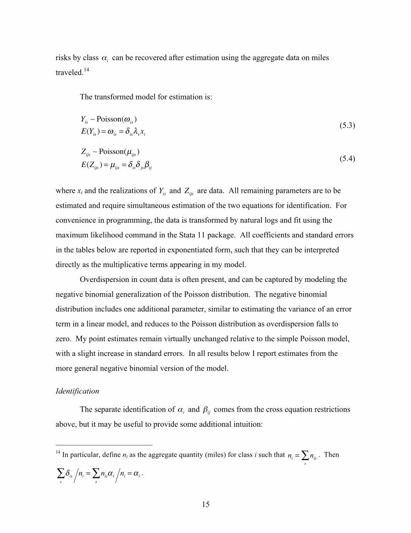
The transformed model for estimation is:

Yis Poisson(ω is )E(Yis ) =ω is = δ isλsxi

(5.3)

Zijs Poisson(µijs )E(Zijs ) = µijs = δ isδ jsβij

(5.4)

where xi and the realizations of Yis and Zijs are data. All remaining parameters are to be

estimated and require simultaneous estimation of the two equations for identification. For

convenience in programming, the data is transformed by natural logs and fit using the

maximum likelihood command in the Stata 11 package. All coefficients and standard errors

in the tables below are reported in exponentiated form, such that they can be interpreted

directly as the multiplicative terms appearing in my model.

Overdispersion in count data is often present, and can be captured by modeling the

negative binomial generalization of the Poisson distribution. The negative binomial

distribution includes one additional parameter, similar to estimating the variance of an error

term in a linear model, and reduces to the Poisson distribution as overdispersion falls to

zero. My point estimates remain virtually unchanged relative to the simple Poisson model,

with a slight increase in standard errors. In all results below I report estimates from the

more general negative binomial version of the model.

Identification

The separate identification of α i and βij comes from the cross equation restrictions

above, but it may be useful to provide some additional intuition:

14 In particular, define ni as the aggregate quantity (miles) for class i such that ni = nis

s∑ . Then

δ iss∑ ni = nisα i

s∑ ni =α i .

16

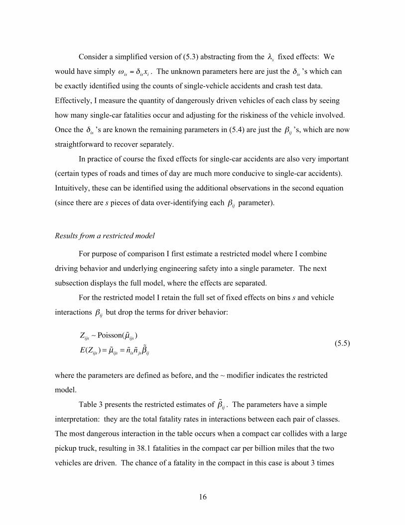
Consider a simplified version of (5.3) abstracting from the λs fixed effects: We

would have simply ω is = δ is xi . The unknown parameters here are just the δ is ’s which can

be exactly identified using the counts of single-vehicle accidents and crash test data.

Effectively, I measure the quantity of dangerously driven vehicles of each class by seeing

how many single-car fatalities occur and adjusting for the riskiness of the vehicle involved.

Once the δ is ’s are known the remaining parameters in (5.4) are just the βij ’s, which are now

straightforward to recover separately.

In practice of course the fixed effects for single-car accidents are also very important

(certain types of roads and times of day are much more conducive to single-car accidents).

Intuitively, these can be identified using the additional observations in the second equation

(since there are s pieces of data over-identifying each βij parameter).

Results from a restricted model

For purpose of comparison I first estimate a restricted model where I combine

driving behavior and underlying engineering safety into a single parameter. The next

subsection displays the full model, where the effects are separated.

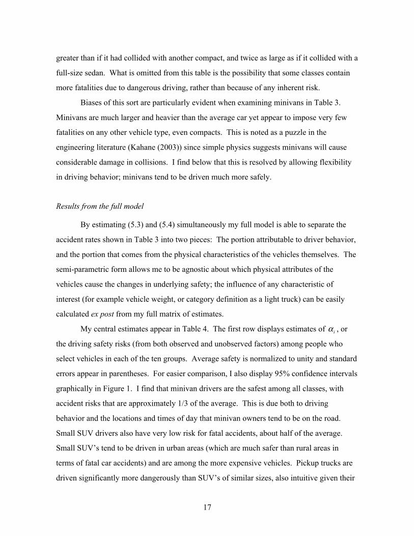
For the restricted model I retain the full set of fixed effects on bins s and vehicle

interactions βij but drop the terms for driver behavior:

Zijs Poisson( µijs )

E(Zijs ) = µijs = nis njs βij

(5.5)

where the parameters are defined as before, and the ~ modifier indicates the restricted

model.

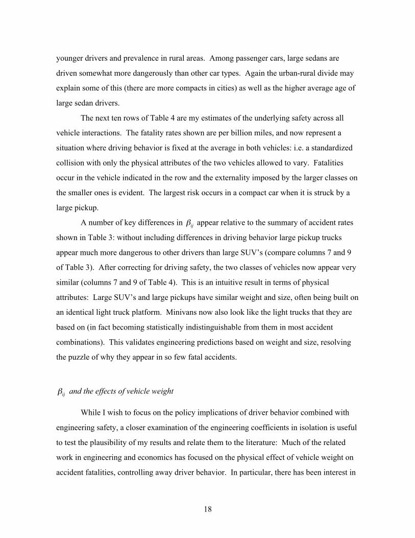
Table 3 presents the restricted estimates of βij . The parameters have a simple

interpretation: they are the total fatality rates in interactions between each pair of classes.

The most dangerous interaction in the table occurs when a compact car collides with a large

pickup truck, resulting in 38.1 fatalities in the compact car per billion miles that the two

vehicles are driven. The chance of a fatality in the compact in this case is about 3 times

17

greater than if it had collided with another compact, and twice as large as if it collided with a

full-size sedan. What is omitted from this table is the possibility that some classes contain

more fatalities due to dangerous driving, rather than because of any inherent risk.

Biases of this sort are particularly evident when examining minivans in Table 3.

Minivans are much larger and heavier than the average car yet appear to impose very few

fatalities on any other vehicle type, even compacts. This is noted as a puzzle in the

engineering literature (Kahane (2003)) since simple physics suggests minivans will cause

considerable damage in collisions. I find below that this is resolved by allowing flexibility

in driving behavior; minivans tend to be driven much more safely.

Results from the full model

By estimating (5.3) and (5.4) simultaneously my full model is able to separate the

accident rates shown in Table 3 into two pieces: The portion attributable to driver behavior,

and the portion that comes from the physical characteristics of the vehicles themselves. The

semi-parametric form allows me to be agnostic about which physical attributes of the

vehicles cause the changes in underlying safety; the influence of any characteristic of

interest (for example vehicle weight, or category definition as a light truck) can be easily

calculated ex post from my full matrix of estimates.

My central estimates appear in Table 4. The first row displays estimates of α i , or

the driving safety risks (from both observed and unobserved factors) among people who

select vehicles in each of the ten groups. Average safety is normalized to unity and standard

errors appear in parentheses. For easier comparison, I also display 95% confidence intervals

graphically in Figure 1. I find that minivan drivers are the safest among all classes, with

accident risks that are approximately 1/3 of the average. This is due both to driving

behavior and the locations and times of day that minivan owners tend to be on the road.

Small SUV drivers also have very low risk for fatal accidents, about half of the average.

Small SUV’s tend to be driven in urban areas (which are much safer than rural areas in

terms of fatal car accidents) and are among the more expensive vehicles. Pickup trucks are

driven significantly more dangerously than SUV’s of similar sizes, also intuitive given their

18

younger drivers and prevalence in rural areas. Among passenger cars, large sedans are

driven somewhat more dangerously than other car types. Again the urban-rural divide may

explain some of this (there are more compacts in cities) as well as the higher average age of

large sedan drivers.

The next ten rows of Table 4 are my estimates of the underlying safety across all

vehicle interactions. The fatality rates shown are per billion miles, and now represent a

situation where driving behavior is fixed at the average in both vehicles: i.e. a standardized

collision with only the physical attributes of the two vehicles allowed to vary. Fatalities

occur in the vehicle indicated in the row and the externality imposed by the larger classes on

the smaller ones is evident. The largest risk occurs in a compact car when it is struck by a

large pickup.

A number of key differences in βij appear relative to the summary of accident rates

shown in Table 3: without including differences in driving behavior large pickup trucks

appear much more dangerous to other drivers than large SUV’s (compare columns 7 and 9

of Table 3). After correcting for driving safety, the two classes of vehicles now appear very

similar (columns 7 and 9 of Table 4). This is an intuitive result in terms of physical

attributes: Large SUV’s and large pickups have similar weight and size, often being built on

an identical light truck platform. Minivans now also look like the light trucks that they are

based on (in fact becoming statistically indistinguishable from them in most accident

combinations). This validates engineering predictions based on weight and size, resolving

the puzzle of why they appear in so few fatal accidents.

and the effects of vehicle weight

While I wish to focus on the policy implications of driver behavior combined with

engineering safety, a closer examination of the engineering coefficients in isolation is useful

to test the plausibility of my results and relate them to the literature: Much of the related

work in engineering and economics has focused on the physical effect of vehicle weight on

accident fatalities, controlling away driver behavior. In particular, there has been interest in

βij

19

both the protection that vehicle weight offers as well as the externality that it imposes on

others. Both of these quantities can be calculated from my estimates of β, but will

necessarily be rough measures due to aggregation.

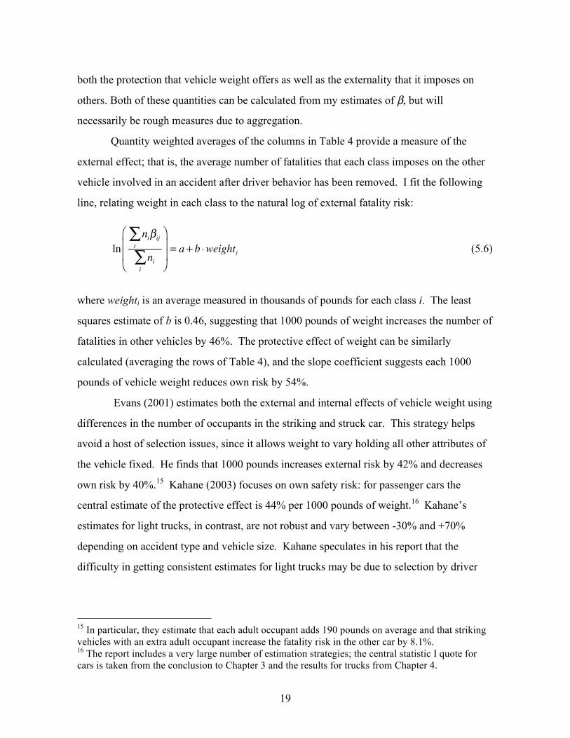
Quantity weighted averages of the columns in Table 4 provide a measure of the

external effect; that is, the average number of fatalities that each class imposes on the other

vehicle involved in an accident after driver behavior has been removed. I fit the following

line, relating weight in each class to the natural log of external fatality risk:

lnniβij

i∑

nii∑

⎛

⎝

⎜⎜

⎞

⎠

⎟⎟= a + b ⋅weighti (5.6)

where weighti is an average measured in thousands of pounds for each class i. The least

squares estimate of b is 0.46, suggesting that 1000 pounds of weight increases the number of

fatalities in other vehicles by 46%. The protective effect of weight can be similarly

calculated (averaging the rows of Table 4), and the slope coefficient suggests each 1000

pounds of vehicle weight reduces own risk by 54%.

Evans (2001) estimates both the external and internal effects of vehicle weight using

differences in the number of occupants in the striking and struck car. This strategy helps

avoid a host of selection issues, since it allows weight to vary holding all other attributes of

the vehicle fixed. He finds that 1000 pounds increases external risk by 42% and decreases

own risk by 40%.15 Kahane (2003) focuses on own safety risk: for passenger cars the

central estimate of the protective effect is 44% per 1000 pounds of weight.16 Kahane’s

estimates for light trucks, in contrast, are not robust and vary between -30% and +70%

depending on accident type and vehicle size. Kahane speculates in his report that the

difficulty in getting consistent estimates for light trucks may be due to selection by driver

15 In particular, they estimate that each adult occupant adds 190 pounds on average and that striking vehicles with an extra adult occupant increase the fatality risk in the other car by 8.1%. 16 The report includes a very large number of estimation strategies; the central statistic I quote for cars is taken from the conclusion to Chapter 3 and the results for trucks from Chapter 4.

20

type. I now have evidence to support this: the selection effects I find among different types

of light trucks are much stronger than those among passenger cars.

Anderson and Auffhammer (2011) also wish to isolate the effects of weight, and

carefully control for accident and driver characteristics. They argue that conditioning on

accident occurrence (either fatal or not) controls for most of the driver selection, such that

the remaining fatality risk can be attributed to the physical characteristics of the vehicle.

They find that 1000 pounds of weight increases external risk by 47%. The rough estimate of

the weight externality contained in my βij parameters is very similar. At least along the

dimension of vehicle weight, this suggests that the multiplicative structure I impose in

equations (3.4) and (3.5) has not restricted the underlying pattern in the data. 6. Policy Simulations

An economic analysis of safety, fuel economy, and fleet composition turns on three

factors: The underlying engineering causes of fatal accidents, the driving risk of the

individuals who choose different vehicle types, and the re-optimization of vehicle choices

that occurs due to the regulation. I recover the first two of these as empirical estimates in

my framework above. The third, modeling which individuals change their car choice as a

result of the standard, is described here.

The first stage of the simulation involves applying the shadow costs of policy to

vehicle choices: Implicitly, existing policy increases the purchases of small cars and

decreases the purchases of large cars in order to meet an average target. Policy also creates

an incentive for technological change that I am assuming does not alter safety in itself; I

instead focus on the changes in fleet composition. All of my empirical measures are per-

mile driven, and that continues to hold in simulation. The vehicle choice model assumes

constant own and cross- price elasticities of demand taken from the literature, and that

consumers re-optimize based on the shadow costs present under different types of fuel

economy standard.

21

The behavior of drivers, a key focus of this paper, also enters the simulation. I first

assume that drivers carry their residual term with them as they switch vehicles. For example

if a minivan or SUV driver switches to a large sedan, that will lower (all else equal) the

fatality rate per mile in sedans. On the other hand, if a pickup truck driver switches to the

same sedan that would increase the fatality rate per mile in sedans. Simulating a movement

of the residual with the driver assumes that exogenous characteristics of drivers make up

most of the safety residual (age, gender, safety of roads in local area, income, alcohol use,

children in the vehicle, etc.).

However, Peltzman (1975) points out that larger, safer vehicles should induce more

risk-taking behavior. Gayer (2004) also makes the case that light trucks and SUV’s are

more difficult to drive, working in the same direction as the Peltzman effect.17 In my

context the Peltzman effect means that a portion of the safety residual should stay with the

vehicle class even as drivers re-optimize. I compute an upper bound on these effects and

allow them to enter a second set of simulations. Intuitively, I find that Peltzman-type effects

make all fuel economy standards look better on safety since we are now arguing that smaller

vehicles themselves cause better driving behavior. Importantly my main policy conclusions,

including the adverse effect of the current standard and the improvement offered by a

unified standard, remain fully robust.

Finally, the farther out of sample I wish to look in simulation (i.e. very extreme

changes to the fleet) the more strain is placed on the empirical estimates. Fortunately, there

is a substantial amount of variation in the fleet already included in the data: For example the

fraction of the fleet that are large pickup trucks varies by more than factor of two across bins

s.18 The changes as the result of fuel economy rules span only a small piece of this

variation.

17 The recent widespread adoption of unibody SUV designs and electronic traction and stability control may reduce this effect. 18 It ranges from 10% (high-income, urban, daytime) to 22% (low-income, rural, night).

22

Simulation Model

I begin with a set of estimates for own and cross-price elasticities of demand among

the 10 vehicle classes. The central-case elasticities I use are shown in Table 5 and come

from Bento et al (2009). I also investigate the robustness of my results to alternative

elasticities. To determine the change in vehicle choices I combine the matrix of elasticities

with the shadow tax implicit in fuel economy regulation.19 The shadow taxes are displayed

in Table 6 for each of the three policies I consider:

1) Extension of the current CAFE rule

The shadow tax in this case is proportional to fuel economy within the light truck

fleet and within the car fleet. This means that large pickups receive a shadow tax while

small pickups receive a shadow subsidy. Similarly large cars receive a shadow tax while

compacts receive a shadow subsidy. There is no incentive to switch from trucks and SUV’s

into cars with this policy, since they are regulated by separate average requirements.

2) Single standard

Here the shadow tax is very simple: The least efficient vehicles receive the highest

tax and the most efficient ones the highest subsidy. All are in proportion to fuel economy.

In general trucks receive a shadow tax (the worse their fuel economy the more so) and cars

receive a shadow subsidy.

3) Footprint-based CAFE standard

This more complicated policy targets fuel economy for vehicles based on their

wheelbase and width. Large footprint vehicles are given a more lenient target, leaving little

or no incentive for manufacturers to change the composition of vehicle types they produce.

The only residual effect on fleet composition will be for classes that are either particularly

efficient relative to their footprint (non-luxury cars) or particularly inefficient relative to

19 Average fuel economy regulation places a shadow tax on vehicles that fall below the average requirement and a shadow subsidy on vehicles that are more efficient than the requirement.

23

their footprint (SUV’s). This implies relatively little switching across vehicle types and

therefore only small changes in safety.

Since the cross-price elasticities describe the full pattern of substitution I can

calculate both the new composition of the fleet and also track the types of drivers as they

switch across vehicles. Depending on which types of drivers are switching into the smaller

vehicles their accident rates per mile can either rise or fall. For example: If the policy

causes a lot of large-pickup drivers to now buy small SUV’s instead, I would predict that the

average driving safety behavior in small SUV’s worsens: The small SUV class will now

contain the relatively safe, urban drivers it originally included, and now also add some

drivers from the more dangerous category that formerly owned large pickups.

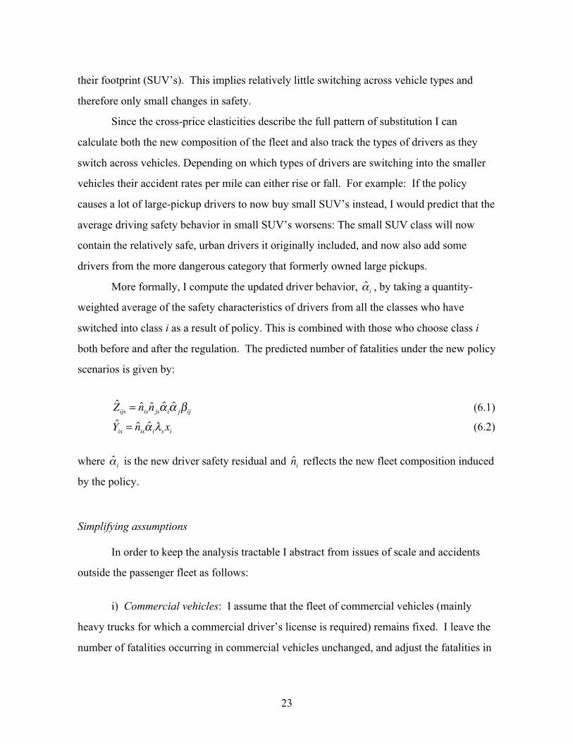
More formally, I compute the updated driver behavior, α i , by taking a quantity-

weighted average of the safety characteristics of drivers from all the classes who have

switched into class i as a result of policy. This is combined with those who choose class i

both before and after the regulation. The predicted number of fatalities under the new policy

scenarios is given by:

Zijs = nisn jsα iα jβij (6.1)

Yis = nisα iλsxi (6.2)

where α i is the new driver safety residual and ni reflects the new fleet composition induced

by the policy. Simplifying assumptions

In order to keep the analysis tractable I abstract from issues of scale and accidents

outside the passenger fleet as follows:

i) Commercial vehicles: I assume that the fleet of commercial vehicles (mainly

heavy trucks for which a commercial driver’s license is required) remains fixed. I leave the

number of fatalities occurring in commercial vehicles unchanged, and adjust the fatalities in

24

passenger vehicles that collide with commercial vehicles using the same risk factors I

estimate for single-car accidents.20

ii) The scale of the fleet and miles driven: It may be that fuel economy rules will

change the total number of cars sold (likely decreasing it) or the number of miles driven

(likely increasing that in a "rebound" effect).21 I focus here on fatalities per mile driven in

order to keep the simulation transparent: to the extent that either the increase in overall miles

or decrease in fleet size is important it will scale total fatalities up or down. The comparison

in policy provisions that I focus on is unaffected by changes in overall scale.22

iii) Pedestrians and bicyclists: About 14% of fatalities involving passenger vehicles

are pedestrians and bicyclists. These fatality rates are nearly identical among cars and light

trucks, consistent with the observation that the mass of the passenger vehicle is many times

larger regardless of its class.23 I therefore assume a constant rate of fatal accidents involving

pedestrians. To the extent that smaller vehicles could reduce pedestrian fatalities – for

example because of better visibility when reversing – both the uncorrected and corrected

results in my model would change by the same amount. Results of policy simulations

The results of the three main policy simulations are contained in Tables 7 through 9.

I compute standard errors for the total change in fatalities in each case by using the delta

20 This is a reasonable approximation since the much larger mass of commercial trucks means collisions with them resemble collisions with fixed objects (albeit at very high speed if the collision occurs head-on). 21 A decrease in quantity might come from cost increases as fuel-saving technologies are introduced. An increase in miles is known as the rebound-effect; better fuel economy means driving becomes cheaper at the margin. 22 Differential changes in driving across vehicle types will have more complicated effects and an extension to the paper could involve a richer simulation model to account for this. These effects would not change the estimation strategy or empirical results. 23 Pedestrian and cyclist fatalities in my data are 2.82 per billion miles for cars and 2.81 per billion miles for light trucks. Within trucks, fatality rates are somewhat higher for larger vehicles. Surprisingly, the opposite effect holds within cars: larger vehicles have lower pedestrian fatality rates.

25

method. The standard errors reflect the estimates of the safety parameters made in this

paper; the hypothetical changes in fleet composition are treated as deterministic.

1) Increment of 1.0 MPG to the current CAFE rules:

The left panel of Table 7 displays the change in total traffic deaths that are predicted

using the restricted model, where driving behavior is not estimated. This restricted model

suggests that CAFE offers an improvement in safety: 135 lives would be saved.

A very different picture emerges when I use the full model, including the selection

on driving behavior at the class level. The central estimate is that the increment to CAFE

will result in 149 additional traffic-related fatalities per year.

It is straightforward to see the intuition behind the reversal in sign: large SUV’s and

pickups (and large sedans) cause and experience a lot of fatal accidents in the data. The

naive restricted model assumes that when you take away these large (and seemingly

dangerous) vehicles an improvement in safety results. Unfortunately I must argue that the

picture is not so favorable: much of the danger in the larger vehicle classes appears to be due

to their drivers, not the cars themselves. When we move those people into smaller vehicles

it does not diminish the risk, and in some cases can even magnify it since smaller vehicles

do more poorly in most single-car accidents.

It is important to point out that the driver effects here are not all habits that we would

fault the drivers themselves for (like running through traffic signals). A significant portion

is simply the urban-rural divide: drivers who currently choose large vehicles tend to live in

rural areas, where accident fatality rates are very high. As rural drivers change to smaller

vehicles the dangers of accidents on rural highways remain. These are very often single-car

accidents, as reflected in the composition of additional fatalities I predict. 2) Unified standard achieving a 1.0 MPG improvement

Table 8 presents results under a unified standard, which has a strikingly different

effect from an increment to current CAFE rules. My full model shows an increase of only 8

fatalities per year under a unified standard. A zero change lies within the confidence

26

bounds. This represents a highly statistically significant improvement over an increment to

current CAFE and comes as the result of two effects canceling each other out in the fleet:

The first effect reiterates the undesirable outcome in the first experiment, that is,

changes within the car fleet and within the truck fleet lead to smaller and lighter vehicles

and increase the number of fatalities.

Recall though that the unified standard adds a second incentive: It encourages

switching away from light trucks and SUV’s and into cars. This second effect improves

overall safety substantially. There appears to be something about light trucks (likely the

height of their center of mass) that makes them more dangerous vehicles than cars, even

after controlling for their drivers. Exchanging an average truck for an average car confers a

large safety benefit to the fleet. It turns out that this improvement almost exactly offsets the

deterioration of safety within the car and truck fleets due to the down-sizing of vehicles. 3) Footprint-based standard

Table 9 presents results under the footprint-based standard that is in effect until

2016. The footprint-based standard discourages most types of composition changes by

shutting down switching both within and across the car and truck fleets. The most

significant changes that remain are movement away from SUV’s and into pickup trucks and

cars; this is due to the relatively small footprint of SUV’s relative to their fuel consumption.

My full model shows a very small deterioration in safety from the footprint standard, with

an increase of only 6 fatalities per year.

It is important to point out that these small safety effects come paired with large

efficiency costs: Fuel savings under the footprint standard must be accomplished almost

exclusively through engine technology, when movement to a smaller and lighter fleet is

likely to be a much cheaper way to save gasoline.

My results on the unified standard are encouraging in this regard: I show that

savings in gasoline from movement to a smaller fleet can come with the same minimal effect

on safety that appears under the footprint standard. As the U.S. presses toward even more

27

fuel efficiency after 2016, changes in fleet composition will prove valuable and can be made

with safety consequences fully in mind. 7. Alternative Models Driver-vehicle specific safety effects correlated with size

Peltzman (1975) argued that safer vehicles (in particular those with seatbelts

installed) will be driven more aggressively as a result of the driver's tradeoff in utility.24

Gayer (2004) presents evidence of a similar effect, where drivers in light trucks appear to

take more risks or have less control when driving. Correlation of this type between vehicle

size and unobserved driving behavior can be expected to improve the safety outcomes

associated with all fuel economy standards, since it assumes that putting people in smaller

vehicles causes safer driving.

I am able to investigate this in the context of my model by further decomposing the

safety residual into two pieces. I define the first piece as being all of the residual driving

safety that is correlated with the own-safety of the vehicle. In that sense it is an upper limit

on the size of the Peltzman effect.25 The second portion is whatever idiosyncratic variation

remains in my estimated driving safety residuals. In the alternative simulations below I

assume that the first portion stays together with the vehicle type (i.e. is adopted by drivers

once they switch to that vehicle). The idiosyncratic part continues to move with the driver.

Table 10 presents the results of these policy experiments. The third column is my upper

bound on the Peltzman effect over all driving safety residuals. The fourth column controls

first for census region (there are more light trucks and dangerous roads in the west) and then

applies the same method to divide the residual into two pieces.

24 Subsequent empirical research has shown this effect may be small, see Cohen and Einav (2003). 25 Unobserved countervailing selection in initial vehicle choice could potentially make the Peltzman effect even larger; these more extreme cases could still be modeled in simulation, possibly using estimates from other studies.

28

As expected, the outcomes in Table 10 show that all fuel economy standards are

improved if drivers become safer when moved to a smaller vehicle. However, even at the

limit defined above I show that the existing fuel economy standard continues to have

adverse effects on safety. Controlling for census region seems reasonable (as driver

residence is unlikely to change with fuel economy standards), and the result becomes closer

to my central case.

More important, the improvement that can be offered by unifying the standard

appears robust to both of the cases where I allow vehicle size to itself influence driving

behavior. This is shown in the final row of the table. Indeed, because the difference in

policies is maintained and overall safety is improved we see that the unified standard begins

to offer substantial improvements in overall safety in the final column of the table. Across

the range of possibilities we see the existing standard causes robust declines in safety, while

a unified standard is at worst neutral with regard to safety, and at best can offer substantial

gains. Estimating driver behavior without using crash test data

It is possible to identify my empirical model (including the measurement of driver

behavior by class) without the use of crash test data, relying instead on the physical

properties of accidents. Accidents between two vehicles of similar mass and speed closely

resemble accidents with fixed objects since both crashes result in rapid deceleration to a

stationary position.26 When vehicles of different mass collide, the heavier vehicle will

decelerate more slowly (pushing the smaller vehicle back) which creates asymmetry in the

degree of injuries.

My alternative identification strategy makes use of this property, setting risk in

single car accidents proportional to the risk in accidents between cars of the same class, βii .

The model described in Section 5 becomes:

26 See Greene (2009). Each vehicle’s change in velocity raised to the 4th power closely predicts injury severity.

29

E(Yis ) = nisα iλsβii (7.1)

E(Zijs ) = nisnjsα iα jβij (7.2)

The restriction on the diagonal elements of β is sufficient for identification.

The first two columns of Table 11 provide a summary of results from my preferred

specification in Section 5. The third column shows the results from estimating (7.1) and

(7.2) above, providing a confirmation of the central findings even under very different

identifying assumptions. The standard errors are much larger in this specification, reflecting

the reduction in data available to the model. Alternative demand elasticities

The general pattern in the simulation, that fewer large vehicles and more small ones

will be sold, is fundamental to a reduction in fuel economy. However, my simulation also

embeds more subtle changes in substitution across classes. For example: Is a driver giving

up a large SUV more likely to buy a small SUV or switch to a small pickup truck?

I investigate the robustness of my simulation results by introducing an entirely

separate set of substitution elasticities, shown in Table 12. These are reported in Kleit

(2004) and are also employed by Austin and Dinan in their 2007 study. The elasticities

derive mainly from survey data on second-choices of new car owners, providing a different

view than the cross-sectional variation used to generate the elasticities in my main

simulation.

The fourth column of Table 11 summarizes the results under the alternative

elasticities. My main findings remain intact, though the effectiveness of a single fuel

economy standard at mitigating safety consequences is somewhat muted relative to my

preferred model.

Additional robustness checks

I also investigate the robustness of my findings in a number of subsamples of the

data. Columns 3 through 5 of Table 13 summarize my main results in various subsamples,

30

with total fatalities scaled by the number of observations used so that the columns are

comparable. 1998 and newer model years

1998 was the first model year where both passenger and driver airbags were required

in all new vehicles. Airbags dramatically alter safety risks, and if their presence also

influences driving behavior or changes relative risks across classes we might expect a

different set of results to emerge. My estimates, however, appear robust in this dimension.

Drivers under 55

There is evidence that elderly drivers may more often be the subjects of fatal traffic

accidents due to their relative frailty.27 This introduces a potential asymmetry in my model:

Older drivers may place themselves at greater risk but don’t necessarily impose this risk on

those around them. I restrict my sample to driver fatalities among those less than 55 years

old and find similar results, suggesting that the frailty effect is not large relative to the

variation in driver behavior overall. Clear weather

My simulations assume that the locational or behavioral factors influencing driver

safety remain with the driver after the change in composition. A potentially important

caveat has to do with weather: If a driver switches away from an SUV, for example, they

may be less likely to drive in the rain or snow. I therefore experiment with a sample limited

to fatalities that occur in clear weather (any weather condition, even fog or mist, is

excluded). Notably, this only removes 10% of observations; 90% of fatal accidents occur in

clear conditions. My results are again unchanged, suggesting that even if there is substantial

behavioral response to weather conditions it would not be relevant to most accident

fatalities.

27 Loughran and Seabury (2007) investigate this issue in detail.

31

8. Conclusions

I introduce a new empirical model of vehicle accidents that provides estimates of

both the behavior of drivers and the underlying risk associated with engineering

characteristics in a single framework. To my knowledge this is the first study to capture

unobserved driver behavior (as fixed effects) and the impact of physical vehicle

characteristics both within and across vehicle categories. The framework has application to

fuel economy policy (the simulations performed here) and also to a much broader set of

policy initiatives. I show that in the case of fuel economy, correctly accounting for driver

behavior significantly alters conclusions about fleet composition and safety.

Two main effects appear in the empirical estimates. First, there is considerable

diversity in driving behavior across vehicle classes: the most dangerous drivers (pickup

truck owners) are nearly four times as likely to be involved in fatal accidents as the safest

drivers (minivan owners) after controlling for the physical safety attributes of their vehicles.

Second, controlling for driver safety produces estimates of the physical safety of interactions

between vehicles that closely mirrors theoretical engineering results. Large and heavy

vehicles are the safest to be inside during an accident but also cause the most external

damage to others. When reduced to the single dimension of vehicle weight, my estimates of

the own and external effects of heavier vehicles match those in the literature closely.

I use these results to address the motivating question relating safety and fuel

economy regulation. I find that the provision in existing CAFE regulation to separate light

trucks and SUVs from passenger cars is harmful to safety: incrementing the standards by 1.0

mile per gallon causes an additional 149 fatalities per year in expectation. The increase in

statistical risk would be valued at 33 cents per gallon of gasoline saved, with any additional

injuries or property damage (assuming they are correlated with fatalities) further increasing

the cost of this type of regulation.28 Intuitively, my estimates measure the degree to which

greater diversity in the vehicle fleet leads to more fatal accidents. Current CAFE standards,

28 The gasoline savings here reflect only fleet composition changes, holding miles driven fixed. To the extent that a “rebound effect” increases miles driven, the safety cost per gallon saved would be even larger.

32

by encouraging light trucks while at the same time making passenger cars smaller and

lighter, increase the diversity of the fleet.

In contrast, I find that a unified fuel economy standard has almost no harmful effect

on safety. Two effects are operating in opposing directions: weight reductions increase risk

while substitution away from light trucks makes the fleet more homogeneous. My model

implicitly compares the relative importance of these two effects, finding that they offset

almost exactly under the shadow costs implied by a uniform fuel economy standard.

Further analysis using the model developed here could uncover additional effects of

interest. For example, a more detailed disaggregation of car classes by manufacturer, fuel

economy, or other attribute could reveal additional ways to adjust fuel economy rules to

protect or even improve safety. The policy simulations might similarly be made richer, with

attention given to inter-firm dynamics or the credit-trading provisions in upcoming federal

regulation.

33

References Anderson, M. and M. Auffhammer (2011), “Pounds That Kill: The External Costs of Vehicle Weight,” University of California, Berkeley working paper. Austin, David and T. Dinan (2005), “Clearing the Air: The Costs and Consequences of Higher CAFE Standards and increased Gasoline Taxes,” Journal of Environmental Economics and Management, 50. Bento, Antonio, Lawrence Goulder, Mark Jacobsen, and Roger von Haefen (2009), "Distributional and Efficiency Impacts of Increased U.S. Gasoline Taxes," American Economic Review, 99(3). Busse, Meghan, Christopher Knittel, and Florian Zettelmeyer (2011), "Pain at the Pump: How Gasoline Prices Affect Automobile Purchasing." Working paper, Massachusetts Institute of Technology. Cohen, Alma and Liran Einav (2003), "The Effect of Mandatory Seat Belt Laws on Driving Behavior and Traffic Fatalities," Review of Economics and Statistics, 85(4), 828-843. Crandall, R.W. and J.D. Graham (1989), “The Effect of Fuel Economy Standards on Automobile Safety,” Journal of Law and Economics 32(1): 97-118.

Environmental Protection Agency and Department of Transportation (2010), Light-Duty Vehicle Greenhouse Gas Emission Standards and Corporate Average Fuel Economy Standards; Final Rule, Federal Register 75(88), May 2010.

Evans, Leonard (2001), “Causal Influence of Car Mass and Size on Driver Fatality Risk.” American Journal of Public Health, 91:1076-81.

Gayer, Ted (2004), “The Fatality Risks of Sport-Utility Vehicles, Vans, and Pickups Relative to Cars,” The Journal of Risk and Uncertainty, 28:2.

Herman, Irving P. (2007), The Physics of the Human Body, New York: Springer, 2007.

Jacobsen, M. (2010), “Evaluating U.S. Fuel Economy Standards In a Model with Producer and Household Heterogeneity,” working paper available from http://econ.ucsd.edu/~m3jacobs/ Jacobsen_CAFE.pdf.

Kahane, C. (2003), Vehicle Weight, Fatality Risk and Crash Compatibility of Model Year 1991-99 Passenger Cars and Light Trucks, NHTSA Technical Report, DOT HS 809 662.

Kleit, Andrew N. (2004), "Impacts of Long-Range Increases in the Corporate Average Fuel Economy (CAFE) Standard." Economic Inquiry 42:279-94.

34

Knittel, Christopher (2011), "The Implied Cost of Carbon Dioxide under the Cash for Clunkers Program," Working paper, Massachusetts Institute of Technology. Levitt, Steven and Jack Porter (2001), “How Dangerous are Drinking Drivers,” Journal of Political Economy, 109:6.

Loughran, David S. and Seth A. Seabury (2007), “Estimating the Accident Risk of Older Drivers,” TR-450- ICJ, Santa Monica: RAND.

National Highway Traffic Safety Administration (2008a), National Motor Vehicle Crash Causation Survey: Report to Congress, DOT HS 811 059, July 2008.

National Highway Traffic Safety Administration (2008b), "Average Fuel Economy Standards - Passenger Cars and Light Trucks Model Years 2011-2015; Proposed Rule," Federal Register: 73(86): 24351-487.

National Highway Traffic Safety Administration (2009), Traffic Safety Facts: A Brief Statistical Summary, DOT HS 811172, June 2009.

National Research Council (2002), Effectiveness and Impact of Corporate Average Fuel Economy (CAFE) Standards, National Academy of Sciences, Washington, DC.

Parry, Ian W. H., and Kenneth A. Small (2005), “Does Britain or the United States Have the Right Gasoline Tax?” American Economic Review, 95(4): 1276–89.

Peltzman, Sam (1975), “The Effects of Automobile Safety Regulation.” The Journal of Political Economy 83(4): 677-725.

Portney, P., I. Parry, H. Gruenspecht and W. Harrington (2003), “The Economics of Fuel Economy Standards,” Journal of Economic Perspectives 17:203–217.

The White House Office of the Press Secretary (2011), President Obama Announces Historic 54.5 MPG Fuel Efficiency Standard, July 29, 2011.

Wenzel, T.P. and M. Ross (2005), “The effects of vehicle model and driver behavior on risk,” Accident Analysis and Prevention 37: 479-494.

White, M. J. (2004), “The ‘Arms Race’ on American Roads: The Effect of Sport Utility Vehicles and Pickup Trucks on Traffic Safety,” The Journal of Law and Economics 47:333-355.

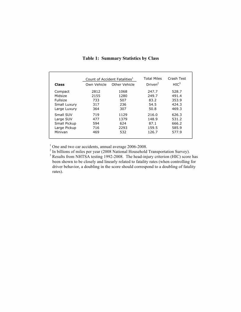
Table 1: Summary Statistics by Class

Count of Accident Fatalities1

Class Own Vehicle Other Vehicle

Compact 2812 1068 247.7 528.7Midsize 2155 1280 249.7 491.4Fullsize 733 507 83.2 353.9Small Luxury 317 236 54.5 424.3Large Luxury 364 307 50.8 469.3

Small SUV 719 1129 216.0 626.3Large SUV 477 1379 148.9 531.2Small Pickup 594 624 87.1 666.2Large Pickup 716 2293 159.5 585.9Minivan 469 532 126.7 577.9

Total Miles

Driven2

Crash Test

HIC3

1 One and two car accidents, annual average 2006-2008. 2 In billions of miles per year (2008 National Household Transportation Survey). 3 Results from NHTSA testing 1992-2008. The head-injury criterion (HIC) score has

been shown to be closely and linearly related to fatality rates (when controlling for driver behavior, a doubling in the score should correspond to a doubling of fatality rates).

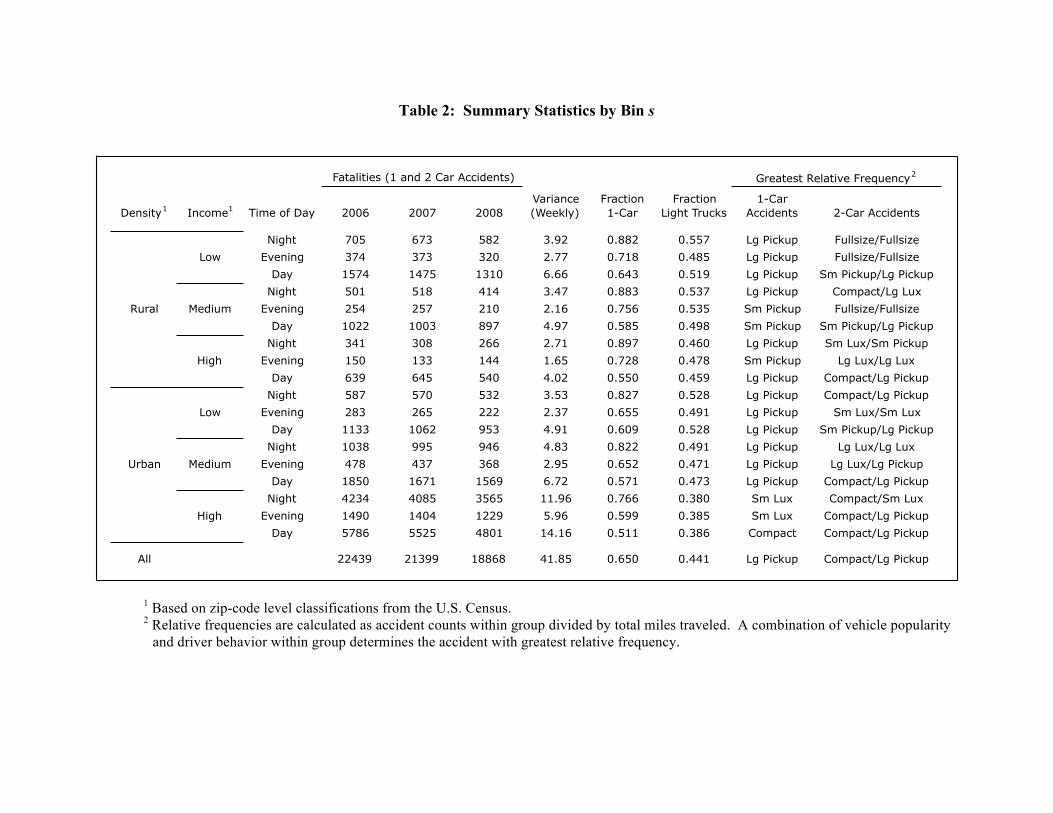
Table 2: Summary Statistics by Bin s

Fatalities (1 and 2 Car Accidents) Greatest Relative Frequency2

Density1 Income1 Time of Day 2006 2007 20081-Car

Accidents 2-Car Accidents

Night 705 673 582 3.92 0.882 0.557 Lg Pickup Fullsize/FullsizeEvening 374 373 320 2.77 0.718 0.485 Lg Pickup Fullsize/Fullsize

Day 1574 1475 1310 6.66 0.643 0.519 Lg Pickup Sm Pickup/Lg PickupNight 501 518 414 3.47 0.883 0.537 Lg Pickup Compact/Lg Lux

Evening 254 257 210 2.16 0.756 0.535 Sm Pickup Fullsize/FullsizeDay 1022 1003 897 4.97 0.585 0.498 Sm Pickup Sm Pickup/Lg Pickup

Night 341 308 266 2.71 0.897 0.460 Lg Pickup Sm Lux/Sm PickupEvening 150 133 144 1.65 0.728 0.478 Sm Pickup Lg Lux/Lg Lux

Day 639 645 540 4.02 0.550 0.459 Lg Pickup Compact/Lg PickupNight 587 570 532 3.53 0.827 0.528 Lg Pickup Compact/Lg Pickup

Evening 283 265 222 2.37 0.655 0.491 Lg Pickup Sm Lux/Sm LuxDay 1133 1062 953 4.91 0.609 0.528 Lg Pickup Sm Pickup/Lg Pickup

Night 1038 995 946 4.83 0.822 0.491 Lg Pickup Lg Lux/Lg LuxEvening 478 437 368 2.95 0.652 0.471 Lg Pickup Lg Lux/Lg Pickup

Day 1850 1671 1569 6.72 0.571 0.473 Lg Pickup Compact/Lg PickupNight 4234 4085 3565 11.96 0.766 0.380 Sm Lux Compact/Sm Lux

Evening 1490 1404 1229 5.96 0.599 0.385 Sm Lux Compact/Lg PickupDay 5786 5525 4801 14.16 0.511 0.386 Compact Compact/Lg Pickup

All 22439 21399 18868 41.85 0.650 0.441 Lg Pickup Compact/Lg Pickup

Variance (Weekly)

Fraction 1-Car

Fraction Light Trucks

Rural

Urban

Low

Medium

High

Low

Medium

High

1 Based on zip-code level classifications from the U.S. Census. 2 Relative frequencies are calculated as accident counts within group divided by total miles traveled. A combination of vehicle popularity

and driver behavior within group determines the accident with greatest relative frequency.

Table 3: Estimates of βij in Restricted Model (No class-level driver safety effects)1

1 Standard errors are shown in parentheses, estimates are from negative binomial estimation of the multi-car accident equation alone, with all class-level safety effects restricted to unity. These coefficients provide a summary of fatal accident rates without controlling for driver behavior.

Compact Midsize FullsizeSmall Luxury

Large Luxury

Small SUV

Large SUV

Small Pickup

Large Pickup Minivan

Compact 12.4 (0.4)

14.9 (0.5)

17.7 (0.9)

12.6 (1.0)

17.2 (1.2)

16.2 (0.5)

26.4 (0.8)

20.2 (1.0)

38.1 (1.0)

12.1 (0.6)

Midsize 8.8 (0.4)

11.8 (0.4)

12.9 (0.8)

9.2 (0.8)

12.8 (1.0)

11.2 (0.5)

20.4 (0.7)

16.5 (0.9)

30.5 (0.9)

8.9 (0.5)

Fullsize 8.7 (0.6)

11.9 (0.8)

16.0 (1.5)

8.8 (1.4)

14.9 (1.9)

11.6 (0.8)

19.0 (1.2)

17.4 (1.5)

30.6 (1.5)

9.8 (1.0)

Small Luxury 8.5 (0.8)

6.5 (0.7)

11.2 (1.6)

11.8 (2.0)

10.8 (2.0)

9.6 (0.9)

12.1 (1.2)

6.9 (1.2)

16.6 (1.4)

5.1 (0.9)

Large Luxury 6.6 (0.7)

8.7 (0.8)

11.6 (1.7)

6.1 (1.5)

11.2 (2.1)

10.3 (1.0)

20.4 (1.6)

13.3 (1.7)

22.9 (1.7)

8.2 (1.1)

Small SUV 3.6 (0.3)

4.2 (0.3)

4.6 (0.5)

4.2 (0.6)

6.8 (0.8)

4.3 (0.3)

7.9 (0.5)

4.9 (0.5)

12.2 (0.6)

3.4 (0.4)

Large SUV 4.2 (0.3)

4.2 (0.3)

3.8 (0.6)

3.7 (0.7)

5.2 (0.8)

3.5 (0.3)

7.9 (0.6)

5.4 (0.6)

11.1 (0.7)

3.7 (0.4)

Small Pickup 8.2 (0.6)

8.4 (0.6)

10.1 (1.2)

4.6 (1.0)

6.6 (1.2)

7.4 (0.6)

14.0 (1.0)

13.0 (1.3)

29.1 (1.4)

7.7 (0.8)

Large Pickup 4.8 (0.3)

5.2 (0.4)

5.9 (0.7)

4.5 (0.7)

6.3 (0.9)

4.4 (0.4)

10.1 (0.7)

7.4 (0.7)

21.5 (0.9)

3.6 (0.4)

Minivan 3.5 (0.3)

3.8 (0.3)

6.1 (0.8)

3.5 (0.7)

3.9 (0.8)

5.0 (0.4)

8.9 (0.7)

7.7 (0.8)

14.4 (0.8)

4.7 (0.5)

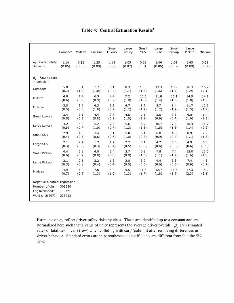
Table 4: Central Estimation Results1

Compact Midsize FullsizeSmall

LuxuryLarge

LuxurySmall SUV

Large SUV

Small Pickup

Large Pickup Minivan

αi: Driver Safety Behavior

1.14 (0.06)

0.98 (0.06)

1.25 (0.08)

1.19 (0.08)

1.05 (0.07)

0.65 (0.04)

1.06 (0.06)

1.09 (0.07)

1.45 (0.08)

0.39 (0.02)

βij: Fatality rate in vehicle i

Compact 5.8 (0.7)

8.1 (1.0)

7.7 (1.0)

5.1 (0.7)

8.3 (1.1)

13.3 (1.6)

13.3 (1.6)

10.9 (1.4)

16.3 (1.9)

16.7 (2.1)

Midsize 4.8 (0.6)

7.4 (0.9)

6.5 (0.9)

4.4 (0.7)

7.2 (1.0)

10.6 (1.3)

11.8 (1.4)

10.1 (1.3)

14.9 (1.8)

14.1 (1.9)

Fullsize 3.8 (0.5)

5.9 (0.8)

6.3 (1.0)

3.5 (0.7)

6.7 (1.2)

8.7 (1.2)

8.7 (1.2)

8.4 (1.2)

11.7 (1.5)

12.2 (1.9)

Small Luxury 3.4 (0.5)

3.1 (0.5)

4.4 (0.8)

3.8 (0.8)

4.5 (1.0)

7.1 (1.1)

5.5 (0.9)

3.5 (0.7)

6.8 (1.0)

6.4 (1.3)

Large Luxury 3.2 (0.5)

4.9 (0.7)

5.2 (1.0)

2.5 (0.7)

5.6 (1.3)

8.7 (1.3)

10.7 (1.5)

7.5 (1.3)

10.4 (1.4)

11.7 (2.2)

Small SUV 2.9 (0.4)

4.0 (0.5)

3.4 (0.6)

3.1 (0.6)

5.8 (1.0)

6.1 (0.8)

6.8 (0.9)

4.5 (0.7)

8.9 (1.1)

7.9 (1.3)

Large SUV 2.1 (0.3)

2.4 (0.3)

1.7 (0.3)

1.7 (0.4)

2.7 (0.5)

3.1 (0.5)

4.2 (0.6)

3.0 (0.5)

4.9 (0.6)

5.3 (0.9)

Small Pickup 4.4 (0.6)

5.2 (0.7)

4.8 (0.8)

2.4 (0.6)

3.7 (0.8)

6.8 (1.0)

7.8 (1.1)

7.4 (1.2)

13.0 (1.6)

11.6 (1.9)

Large Pickup 2.1 (0.3)

2.6 (0.3)

2.2 (0.4)

1.8 (0.4)

2.8 (0.5)

3.2 (0.5)

4.4 (0.6)

3.3 (0.5)

7.4 (0.9)

4.3 (0.7)

Minivan 4.9 (0.7)

6.0 (0.9)

7.6 (1.3)

4.4 (1.0)

5.5 (1.3)

11.8 (1.7)

12.7 (1.8)

11.6 (1.9)

17.3 (2.3)

18.2 (3.1)

Negative binomial regressionNumber of obs: 308880Log likelihood: -89321Wald chi2(297): 233212

1 Estimates of α i reflect driver safety risks by class. These are identified up to a constant and are normalized here such that a value of unity represents the average driver overall. βij are estimated rates of fatalities in car i (row) when colliding with car j (column) after removing differences in driver behavior. Standard errors are in parentheses; all coefficients are different from 0 at the 5% level.

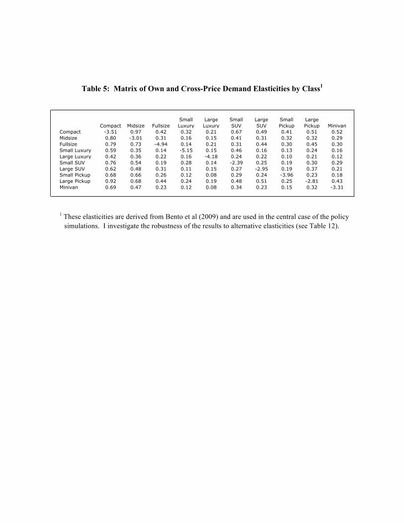
Table 5: Matrix of Own and Cross-Price Demand Elasticities by Class1

1 These elasticities are derived from Bento et al (2009) and are used in the central case of the policy simulations. I investigate the robustness of the results to alternative elasticities (see Table 12).

Compact Midsize FullsizeSmall Luxury

Large Luxury

Small SUV

Large SUV

Small Pickup

Large Pickup Minivan

Compact -3.51 0.97 0.42 0.32 0.21 0.67 0.49 0.41 0.51 0.52Midsize 0.80 -3.01 0.31 0.16 0.15 0.41 0.31 0.32 0.32 0.29Fullsize 0.79 0.73 -4.94 0.14 0.21 0.31 0.44 0.30 0.45 0.30Small Luxury 0.59 0.35 0.14 -5.15 0.15 0.46 0.16 0.13 0.24 0.16Large Luxury 0.42 0.36 0.22 0.16 -4.18 0.24 0.22 0.10 0.21 0.12Small SUV 0.76 0.54 0.19 0.28 0.14 -2.39 0.25 0.19 0.30 0.29Large SUV 0.62 0.48 0.31 0.11 0.15 0.27 -2.95 0.19 0.37 0.21Small Pickup 0.68 0.66 0.26 0.12 0.08 0.29 0.24 -3.96 0.23 0.18Large Pickup 0.92 0.68 0.44 0.24 0.19 0.48 0.51 0.25 -2.81 0.43Minivan 0.69 0.47 0.23 0.12 0.08 0.34 0.23 0.15 0.32 -3.31

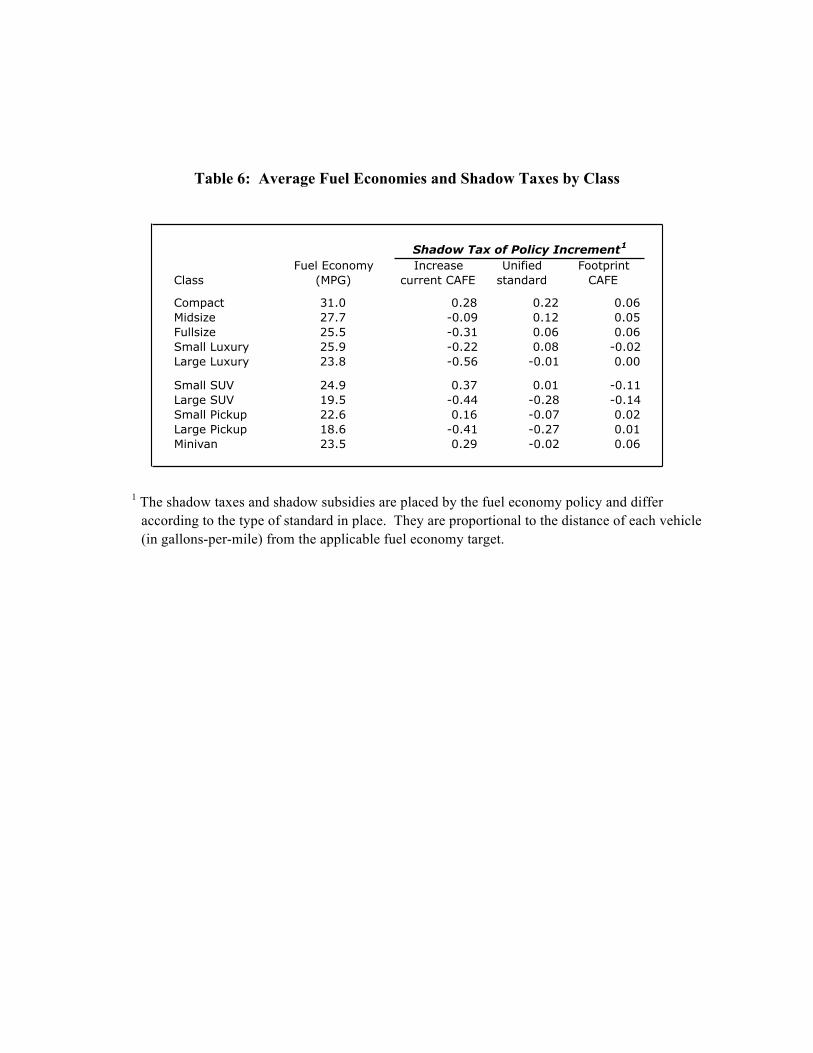
Table 6: Average Fuel Economies and Shadow Taxes by Class

Shadow Tax of Policy Increment1

ClassFuel Economy

(MPG)Increase

current CAFEUnified

standardFootprint

CAFE

Compact 31.0 0.28 0.22 0.06Midsize 27.7 -0.09 0.12 0.05Fullsize 25.5 -0.31 0.06 0.06Small Luxury 25.9 -0.22 0.08 -0.02Large Luxury 23.8 -0.56 -0.01 0.00

Small SUV 24.9 0.37 0.01 -0.11Large SUV 19.5 -0.44 -0.28 -0.14Small Pickup 22.6 0.16 -0.07 0.02Large Pickup 18.6 -0.41 -0.27 0.01Minivan 23.5 0.29 -0.02 0.06

1 The shadow taxes and shadow subsidies are placed by the fuel economy policy and differ according to the type of standard in place. They are proportional to the distance of each vehicle (in gallons-per-mile) from the applicable fuel economy target.

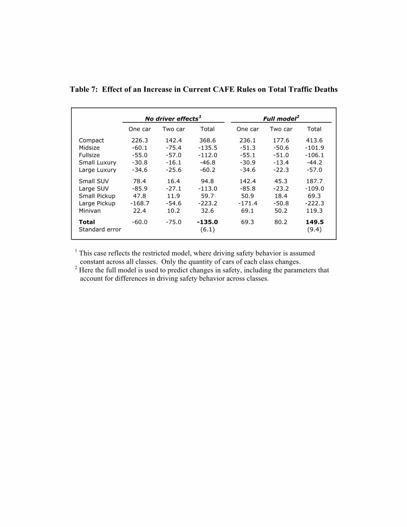
Table 7: Effect of an Increase in Current CAFE Rules on Total Traffic Deaths

No driver effects1 Full model2

One car Two car Total One car Two car Total

Compact 226.3 142.4 368.6 236.1 177.6 413.6Midsize -60.1 -75.4 -135.5 -51.3 -50.6 -101.9Fullsize -55.0 -57.0 -112.0 -55.1 -51.0 -106.1Small Luxury -30.8 -16.1 -46.8 -30.9 -13.4 -44.2Large Luxury -34.6 -25.6 -60.2 -34.6 -22.3 -57.0

Small SUV 78.4 16.4 94.8 142.4 45.3 187.7Large SUV -85.9 -27.1 -113.0 -85.8 -23.2 -109.0Small Pickup 47.8 11.9 59.7 50.9 18.4 69.3Large Pickup -168.7 -54.6 -223.2 -171.4 -50.8 -222.3Minivan 22.4 10.2 32.6 69.1 50.2 119.3

Total -60.0 -75.0 -135.0 69.3 80.2 149.5Standard error (6.1) (9.4)

1 This case reflects the restricted model, where driving safety behavior is assumed constant across all classes. Only the quantity of cars of each class changes.

2 Here the full model is used to predict changes in safety, including the parameters that account for differences in driving safety behavior across classes.

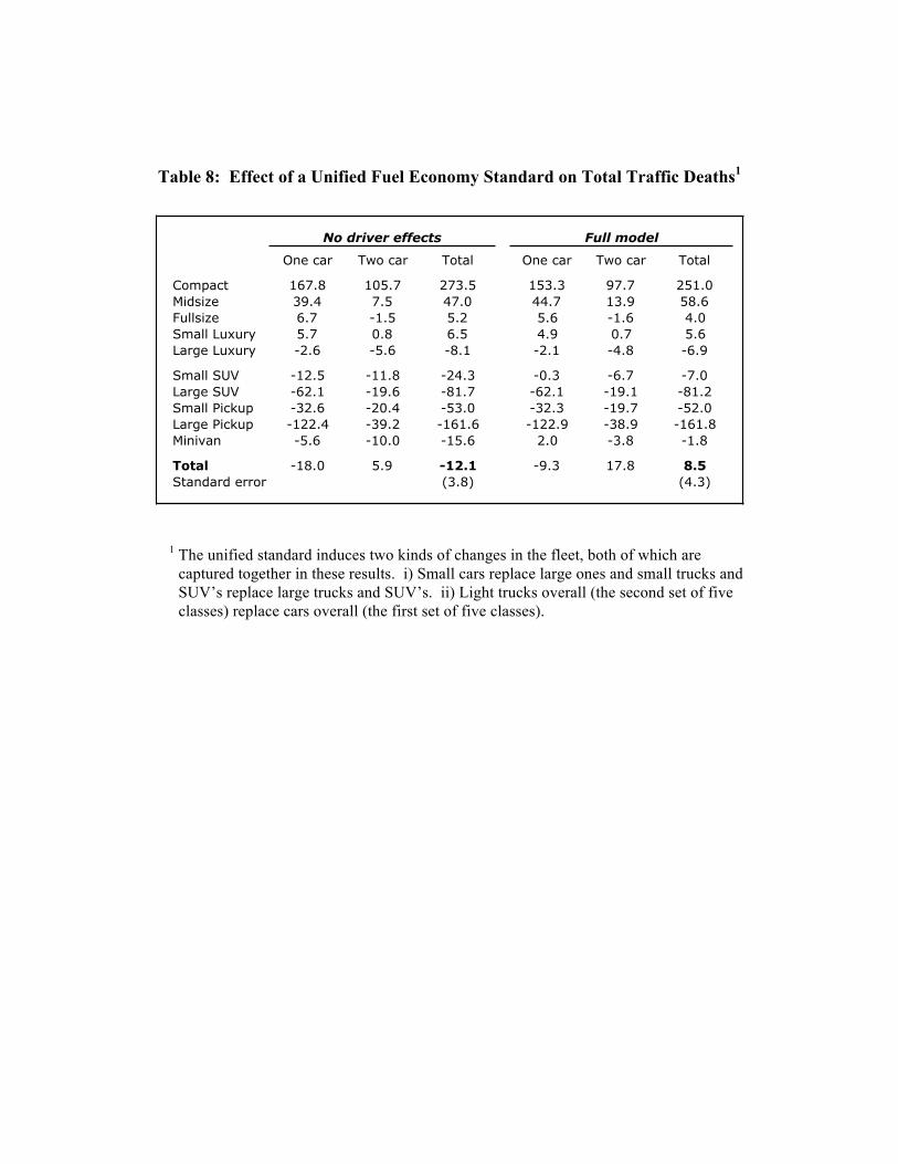
Table 8: Effect of a Unified Fuel Economy Standard on Total Traffic Deaths1

No driver effects Full model

One car Two car Total One car Two car Total

Compact 167.8 105.7 273.5 153.3 97.7 251.0Midsize 39.4 7.5 47.0 44.7 13.9 58.6Fullsize 6.7 -1.5 5.2 5.6 -1.6 4.0Small Luxury 5.7 0.8 6.5 4.9 0.7 5.6Large Luxury -2.6 -5.6 -8.1 -2.1 -4.8 -6.9

Small SUV -12.5 -11.8 -24.3 -0.3 -6.7 -7.0Large SUV -62.1 -19.6 -81.7 -62.1 -19.1 -81.2Small Pickup -32.6 -20.4 -53.0 -32.3 -19.7 -52.0Large Pickup -122.4 -39.2 -161.6 -122.9 -38.9 -161.8Minivan -5.6 -10.0 -15.6 2.0 -3.8 -1.8

Total -18.0 5.9 -12.1 -9.3 17.8 8.5Standard error (3.8) (4.3)

1 The unified standard induces two kinds of changes in the fleet, both of which are captured together in these results. i) Small cars replace large ones and small trucks and SUV’s replace large trucks and SUV’s. ii) Light trucks overall (the second set of five classes) replace cars overall (the first set of five classes).

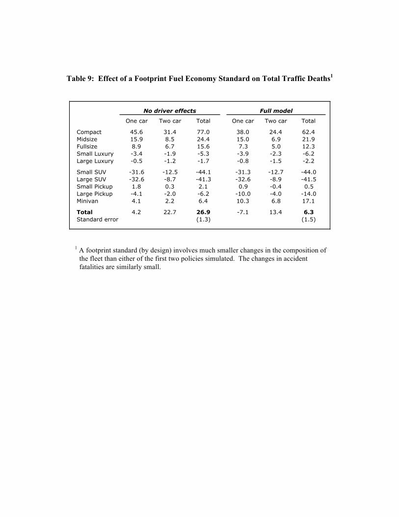
Table 9: Effect of a Footprint Fuel Economy Standard on Total Traffic Deaths1

No driver effects Full model

One car Two car Total One car Two car Total

Compact 45.6 31.4 77.0 38.0 24.4 62.4Midsize 15.9 8.5 24.4 15.0 6.9 21.9Fullsize 8.9 6.7 15.6 7.3 5.0 12.3Small Luxury -3.4 -1.9 -5.3 -3.9 -2.3 -6.2Large Luxury -0.5 -1.2 -1.7 -0.8 -1.5 -2.2

Small SUV -31.6 -12.5 -44.1 -31.3 -12.7 -44.0Large SUV -32.6 -8.7 -41.3 -32.6 -8.9 -41.5Small Pickup 1.8 0.3 2.1 0.9 -0.4 0.5Large Pickup -4.1 -2.0 -6.2 -10.0 -4.0 -14.0Minivan 4.1 2.2 6.4 10.3 6.8 17.1

Total 4.2 22.7 26.9 -7.1 13.4 6.3Standard error (1.3) (1.5)

1 A footprint standard (by design) involves much smaller changes in the composition of the fleet than either of the first two policies simulated. The changes in accident fatalities are similarly small.

Table 10: Peltzman Effects and the Influence of a Driver-Vehicle Specific Residual1

No driver effects

Full model (central)

Peltzman effect

(upper limit)

Peltzman within census divisions

(upper limit)

Current CAFE within fleet

-135.02 (6.15)

149.47 (9.36)

69.80 (9.36)

101.72 (9.36)

Unified standard -12.14 (3.81)

8.50 (4.35)

-57.00 (4.35)

-64.43 (4.35)

Footprint-based standard

26.88 (1.28)

6.27 (1.52)

-18.94 (1.52)

-4.49 (1.52)

Improvement offered by unified standard

-122.9 141.0 126.8 166.1

1 The values in the right two columns allow driving behavior to improve as drivers

switch to smaller vehicle classes. They are upper limits in the sense that all of the correlation between estimated driver behavior and size is attributed to the vehicle (e.g. large vehicles are driven more aggressively or are more difficult to control). As expected, all safety outcomes from CAFE improve in these columns. The sign of the effect on the current CAFE standard is preserved and the improvement offered by a unified standard is robust.

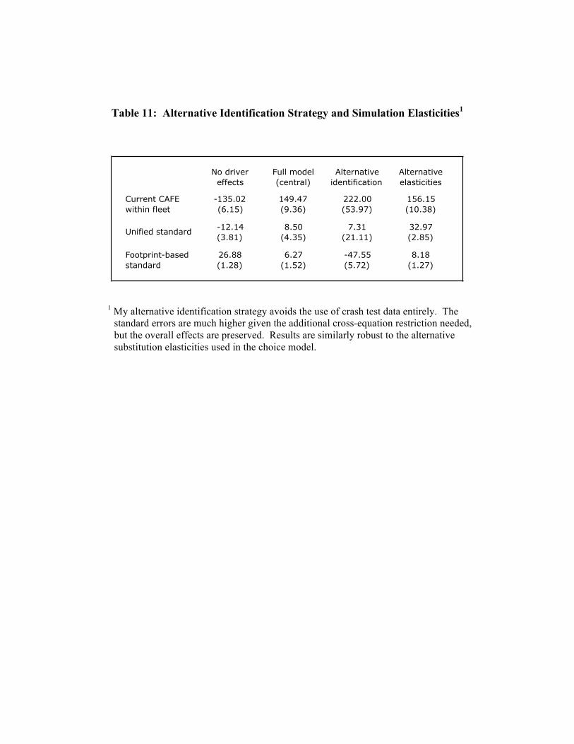
Table 11: Alternative Identification Strategy and Simulation Elasticities1

No driver effects

Full model (central)

Alternative identification

Alternative elasticities

Current CAFE within fleet

-135.02 (6.15)

149.47 (9.36)

222.00 (53.97)

156.15 (10.38)

Unified standard -12.14 (3.81)

8.50 (4.35)

7.31 (21.11)

32.97 (2.85)

Footprint-based standard

26.88 (1.28)

6.27 (1.52)

-47.55 (5.72)

8.18 (1.27)

1 My alternative identification strategy avoids the use of crash test data entirely. The

standard errors are much higher given the additional cross-equation restriction needed, but the overall effects are preserved. Results are similarly robust to the alternative substitution elasticities used in the choice model.

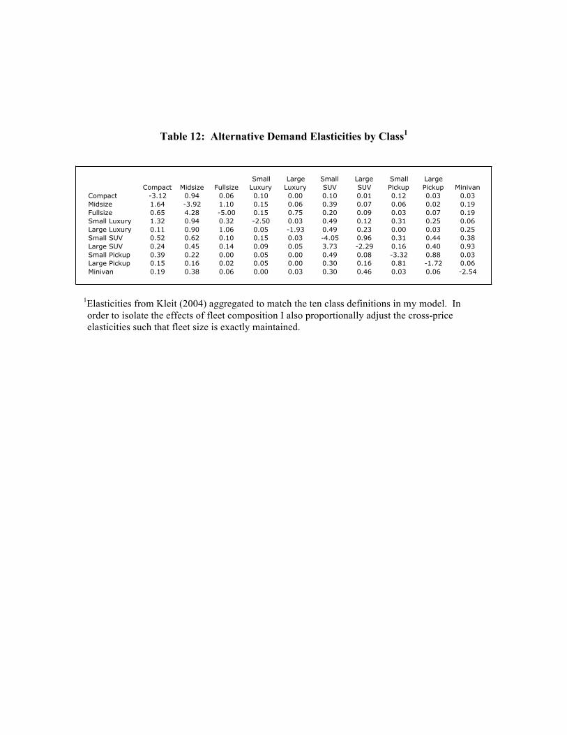
Table 12: Alternative Demand Elasticities by Class1

Compact Midsize FullsizeSmall

LuxuryLarge

LuxurySmall SUV

Large SUV

Small Pickup

Large Pickup Minivan

Compact -3.12 0.94 0.06 0.10 0.00 0.10 0.01 0.12 0.03 0.03Midsize 1.64 -3.92 1.10 0.15 0.06 0.39 0.07 0.06 0.02 0.19Fullsize 0.65 4.28 -5.00 0.15 0.75 0.20 0.09 0.03 0.07 0.19Small Luxury 1.32 0.94 0.32 -2.50 0.03 0.49 0.12 0.31 0.25 0.06Large Luxury 0.11 0.90 1.06 0.05 -1.93 0.49 0.23 0.00 0.03 0.25Small SUV 0.52 0.62 0.10 0.15 0.03 -4.05 0.96 0.31 0.44 0.38Large SUV 0.24 0.45 0.14 0.09 0.05 3.73 -2.29 0.16 0.40 0.93Small Pickup 0.39 0.22 0.00 0.05 0.00 0.49 0.08 -3.32 0.88 0.03Large Pickup 0.15 0.16 0.02 0.05 0.00 0.30 0.16 0.81 -1.72 0.06Minivan 0.19 0.38 0.06 0.00 0.03 0.30 0.46 0.03 0.06 -2.54

1Elasticities from Kleit (2004) aggregated to match the ten class definitions in my model. In order to isolate the effects of fleet composition I also proportionally adjust the cross-price elasticities such that fleet size is exactly maintained.

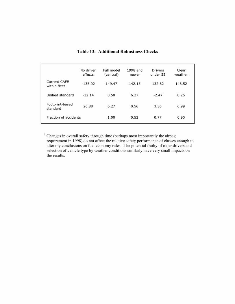
Table 13: Additional Robustness Checks

No driver effects

Full model (central)

1998 and newer

Drivers under 55

Clear weather

Current CAFE within fleet

-135.02 149.47 142.15 132.82 148.52

Unified standard -12.14 8.50 6.27 -2.47 8.26

Footprint-based standard

26.88 6.27 0.56 3.36 6.99

Fraction of accidents 1.00 0.52 0.77 0.90

1 Changes in overall safety through time (perhaps most importantly the airbag requirement in 1998) do not affect the relative safety performance of classes enough to alter my conclusions on fuel economy rules. The potential frailty of older drivers and selection of vehicle type by weather conditions similarly have very small impacts on the results.

Figure 1: Estimates of α i in Full Model1

0

0.2

0.4

0.6

0.8

1

1.2

1.4

1.6

Compa

ct

Midsize

Fulls

ize

Small

Luxu

ry

Larg

e Lux

ury

Small

SUV

Larg

e SUV

Small

Pick

up

Larg

e Pick

up

Miniva

n

1 Values are taken from the first row of Table 4 and bars indicate 95% confidence intervals. The average driving safety behavior is normalized to 1.