functions of a complex variable and integral...
TRANSCRIPT
Functions of a Complex Variable
and Integral Transforms
Department of Mathematics
Zhou Lingjun

Textbook
Functions of Complex Analysis with Applications
to Engineering and Science, 3rd Edition. A. D.
Snider & E. B. Saff.
References
Complex Analysis, Third Edition, Lars V.Ahlfors

What is the course about?
• The main roles of this course are single variable functions which
are defined on a set of complex numbers.
• We concentrate on a group of beautiful functions, which are called
analytic functions.
• Using the property of analytic functions, many difficult problems
can be solved.
• The integral transforms are based on the single complex variable
functions, which are powerful tools to solve differential equations.

The History of Numbers
• Natural numbers are created to count.
• For fixed natural numbers m > n, the equation m + x = n willnot have a solution in natural numbers. In order to solve suchequations, the negative integers are introduced.
• For fixed integer n and nonzero integer m, the equation mx = nmay not have a solution in integer numbers. In order to solvesuch equations, the rational numbers are introduced.
• For fixed positive rational number q, the equation x2 = q may nothave a solution in the rational numbers. In order to solve suchequations, the real numbers are introduced.
• For fixed negative real number q, the equation x2 = q will not havea solution in the real numbers. In order to solve such equations,the complex number are introduced.

Chapter 1
Complex Numbers

1.1 The Algebra of Complex
Numbers
Introduction to Complex Numbers
• We call z = x+ iy a complex number, where x, y are real numbersand i is a symbol of character.
• The real number x, y are called the real and imaginary parts of z,which are denoted as Re z and Im z respectively.
• Two complex numbers are equal iff Re z1 = Re z2 and Im z1 =Im z2.
• The set of all the complex numbers is denoted as C.
• We use the real number x to denote x+ i0 in brief, in which sensethe set of real numbers R can be regarded as a subset of the setC.
• We use iy to denote 0+iy in brief, which is called a pure imaginarynumber.

Fundamental Operations
• Addition and Multiplication: For z1 = x1 + iy1, z2 = x2 + iy2, wedefine
z1 + z2 = (x1 + x2) + i(y1 + y2),
z1z2 = (x1x2 − y1y2) + i(x1y2 + x2y1).
• The definition is natural, since i is treated as a symbol and i2 isreplaced by −1.
• For z = x+iy, denote −z = (−x)+i(−y) = (−1)z, then z+(−z) =0.
• For z = x+ iy 6= 0, denote z−1 = x−iyx2+y2, then zz−1 = 1.

• Subtraction and Division: For z1, z2 ∈ C, we define z1 − z2 =
z1 + (−z2). Moreover if z2 6= 0, we define z1z2
= z1 · z−12 .
• Operational Rules
Commutative Law of Addition z1 + z2 = z2 + z1
Associative Law of Addition (z1 + z2) + z3 = z1 + (z2 + z3)
Commutative Law of Multiplication z1z2 = z2z1
Associative Law of Multiplication (z1z2)z3 = z1(z2z3)
Distributive Law (z1 + z2)z3 = z1z3 + z2z3
• The complex number set C with the addition and multiplication
defined above is a field.

1.2 Point Representation of Complex Numbers
• Each complex number z = x+ iy can be associated a point (x, y)
in the plane.
• For z = x + iy, we define |z| =√x2 + y2, which is called the
modulus (or absolute value or norm) of z.
• For x = x+ iy, the complex conjugate of z is defined by z = x− iy.
• z = ¯z. z is real if and only if z = z.

Vectors and Polar Forms
• Vectors and Complex numbers: A complex number z = x + iy
can be regarded as a vector. z can be expressed in Cartesian
coordinate (x, y), or in terms of the polar coordinate (r, θ)

• r = |z|. θ is determined up to an integer multiple of 2π. We call
the value of any of these angles an argument of z, denoted Arg z.
• The argument lies in the interval (−π, π) is known as the principle
value of the argument, denoted arg z.
• Polar Form: z = r(cos θ + sin θ).
• Triangle Inequality: ||z1| − |z2|| ≤ |z1 + z2| ≤ |z1|+ |z2|.
• |z1z2| = |z1| · |z2|, |z1z2| = |z1|
|z2|.
• Arg (z1 + z2) = Arg z1 + Arg z2.
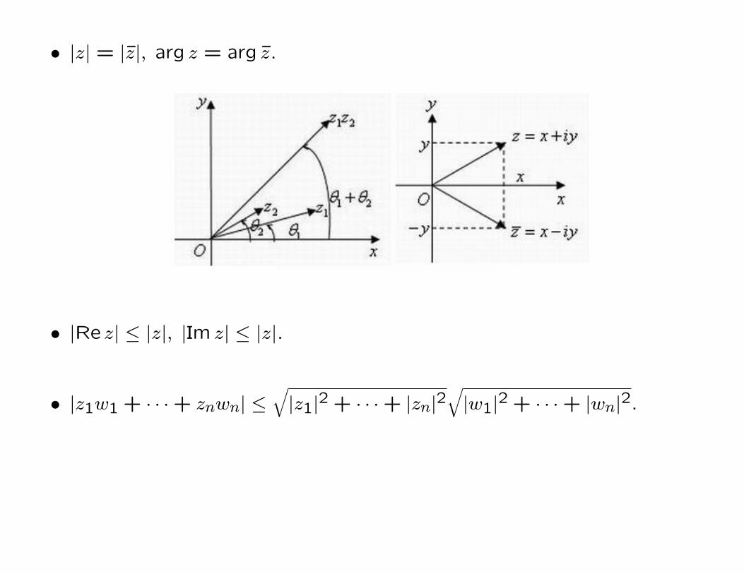
• |z| = |z|, arg z = arg z.
• |Re z| ≤ |z|, |Im z| ≤ |z|.
• |z1w1 + · · ·+ znwn| ≤√|z1|2 + · · ·+ |zn|2
√|w1|2 + · · ·+ |wn|2.
Powers and Roots
• For z and a positive integer n, we define zn = z · · · z︸ ︷︷ ︸n
.
• For nonzero z and a positive integer n, we define z−n = (zn)−1.
• De Moivre Formula. If z = r(cos θ + sin θ) and n is an integer,
then zn = rn(cosnθ + sinnθ).
• For nonzero z = r(cos θ + sin θ) and a positive integer nthe nth
roots of z are given by the n complex numbers
zk = n√r
[cos
(θ
n+
2kπ
n
)+ i sin
(θ
n+
2kπ
n
)], k = 0,1, . . . , n− 1.
• The roots form the vertices of a regular polygon.

1.3 Planar Sets
• We call the set Nδ(z0) = z||z − z0| < δ an open disk of z0.
• A point z0 is called an interior point of the set S, if there exists
an open disk of z0 which is contained in S.
• A set S is called an open set, if each point of S is an interior point
of S.
• A point z0 is called an exterior point of the set S, if z0 is the
interior point of Sc (the complement set of S).
• A point z0 is called a boundary point of the set S, if z0 is neither
an interior point nor an exterior point. The set of all boundary
points of E is called the boundary of S, which is denoted by ∂S.
• Denote S = S ∪ ∂S, which is called the closure of S.

• A open set D is called a domain (or region) if it is connected,
which means each pair z1, z2 ∈ D can be joined by a polygonal
path lying in D.
• In our lectures, we always use D to denote a domain without
further interpretation.
• Theorem. Suppose u(x, y) is a real-valued function defined in a
domain D. If the first partial derivatives of u satisfy
∂u
∂x=∂u
∂y= 0
at all point of D, then u is a constant in D.

Contours
• A curve γ in domain D is the range of a continuous mapping z(t)from [a, b] to D. z(t) is called a parametrization of γ.
• A curve γ is said to be a smooth arc if it is the range of somecontinuous complex-valued function z = z(t), (a ≤ t ≤ b) thatsatisfies the following conditions:
1. z(t) has a continuous derivative on [a, b],
2. z′(t) never vanishes on [a, b],
3. z(t) is one-to-one on [a, b].
A curve γ is called a smooth closed curve if it is the range ofsome continuous complex-valued function z = z(t), (a ≤ t ≤ b),satisfying conditions (1) and (2) and the following:

3’. z(t) is one-to-one on [a, b), but z(b) = z(a) and z′(b) = z′(a).
The phrase smooth curve means either a smooth arc or a smooth
closed curve.
• A smooth arc is called a directed smooth arc if one of its endpoints
is specified as the initial point.
A smooth closed curve whose points have been ordered is called
a directed smooth closed curve.
The phrase directed smooth curve means either a directed smooth
arc or a directed smooth closed curve.
• A contour Γ is either a single point z0 or a finite sequence of direct-
ed smooth curve (γ1, γ2, . . . , γn) such that the terminal point of γkcoincides with the initial point of γk+1 for each k = 1,2, . . . , n−1.
In this case one can write Γ = γ1 + γ2 + · · ·+ γn.

Γ is said to be a closed contour or a loop if its initial and terminalpoints coincide.
A simple closed contour is a closed contour with no multiple pointsother than its initial-terminal point.
• Jordan Curve Theorem. Any simple closed contour divides theplane into exactly two domains, each having the curve as itsboundary. One of these domains, called the interior, is bound-ed and the other, called exterior is unbounded.
• The direction along a simple closed contour Γ can be completelyspecified by declaring its initial-terminal point and stating whichdomain lies to the left of an observer tracing out the points inorder. When the interior domain lies to the left, we say that Γ ispositively oriented. Otherwise Γ is said to be negatively oriented.
A positively orientation generalizes the concept of counterclock-wise motion.
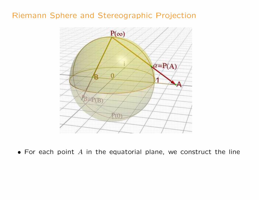
Riemann Sphere and Stereographic Projection
• For each point A in the equatorial plane, we construct the line

passing through the the north pole N = (0,0,1) of the unit sphere
and A. This line pierces the unit sphere in exactly one point P (A).
• For each point on the sphere other than the north pole N , we
construct the line passing through these two points. This line
pierces the equatorial plane in exactly one point. Therefore the
map P , called stereographic projection, is a bijection from the
equatorial plane to the unit sphere without the north pole.
• If we identify the equatorial plane as the complex plane, the unit
sphere is call the Riemann sphere.
• N does not arise as the projection of any point of in the complex
plane. However we find P−1(z) tends to N as |z| → ∞. We set
∞ is the image of N under the stereographic projection, and the
complex plane together with ∞ is called the extended complex
plane, which is denoted by C.

1.4 Functions of a Complex Variable
• In this lecture, we usually consider a function w = f(z) defined on
a subset of the complex plane C, and its range also lies in C.
• Let z = x+ iy (x, y ∈ R), then f(z) can be written as
f(z) = u(x, y) + iv(x, y),
where u(x, y), v(x, y) are real-valued functions.
• Unlike the real variable function, we cannot draw a graph of a
complex variable function, since both variable z and value w are
located in a plane. We usually draw the z and w plane separately.

Chapter 2
Analytic Functions
2.1 Limits and continuity
• The definitions of limits and continuity in the sense of complexvariable functions are the same as the relevant definitions in cal-culus.
• The properties of limits are also the same as the relevant proper-ties in calculus.
• The function f(z) is continuous iff both u(x, y) and v(x, y), re-garding as real variable functions, are continuous.
• A continuous complex variable function do not have more specialproperties than a continuous real variable function.

2.2 Analyticity
• Let f be a complex-valued function defined in a neighborhood ofz0. Then the derivative of f at z0 is given by
f ′(z0) = limz→z0
f(z)− f(z0)
z − z0,
provided this limit exists. Such an f is said to be differentiable atz0.
• The properties of derivatives are almost the same as the relevantproperties in calculus, for example the chain rule.
• A function f is called analytic in a domain D ⊂ C if it has aderivative at each point in D.
• If f(z) is analytic on the whole complex plane, then it is said tobe entire.

The Cauchy-Riemann Equations
• Theorem 1. The necessary condition for a function f(z) = u(x, y)+
iv(x, y) to be differentiable at z0 is that the Cauchy-Riemann e-
quations
∂u
∂x=∂v
∂y,
∂u
∂y= −
∂v
∂x
hold at z0.
• Theorem 2. Let f be a complex-valued function defined in some
open set G containing z0. If the first partial derivatives of u and
v exist in G, and satisfy the the Cauchy-Riemann equations at z0,
then f is differentiable at z0. (The proof is highly involved.)
• Corollary. f is analytic in some region D if and only if u, v satisfy
the Cauchy-Riemann equations in D.

2.4 The Elementary Functions
1. Exponential function.
• ez is an entire function, and (ez)′ = ez.
• ez is periodic function, and the period is 2πi.
• ez1ez2 = ez1+z2.
• ez is one-to-one on each strip x+ iy : a < y < a+ h, h < 2π.
2. The Trigonometric Functions
For z ∈ C, we define
cos z =eiz + e−iz
2, sin z =
eiz − e−iz
2i.
• Most formulae for cos z and sin z hold in C.
• sin z and cos z are periodic functions, and the period is 2π.
• sin z and cos z are entire function, and
(sin z)′ = cos z, (cos z)′ = − sin z.
• sin z and cos z are boundless, that is to say that
| sin z| ≤ 1, | cos z| ≤ 1
do not hold in C.
3. The Hyperbolic Functions
For any z ∈ C, we define
cosh z =ez + e−z
2, sinh z =
ez − e−z
2.
• cosh2 z − sinh2 z = 1.
• sinh z and cosh z are periodic functions, and the period is 2πi.
• sin z and cos z are entire function, and
(sinh z)′ = cosh z, (cosh z)′ = − sinh z.
• sin iz = i sinh z, sinh iz = i sin z, cos iz = cosh z, cosh iz = cos z.

4. The Logarithmic Function
For any nonzeoro z ∈ C, we define
Log z = log |z|+ iArg z, log z = log |z|+ i arg z.
• Log z is a multiple valued function, and it solves the equation
ew = z with respect of w.
• log z is called the principal value of Log z.
• log z is analytic in C \ Re z ≤ 0., and (log z)′ = 1z .
• log z is not continuous in the set Re z < 0.
• Remark The formulae for log z for real variable do not always hold
for complex variable. We should treat it very carefully.
5. Complex Powers
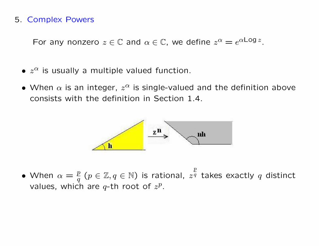
For any nonzero z ∈ C and α ∈ C, we define zα = eαLog z.
• zα is usually a multiple valued function.
• When α is an integer, zα is single-valued and the definition above
consists with the definition in Section 1.4.
• When α = pq (p ∈ Z, q ∈ N) is rational, z
pq takes exactly q distinct
values, which are q-th root of zp.

• When α is irrational, zα takes infinity many values.
• In order to make zα be single-valued, we need to restrict Log z
on a single-valued branch. For example we define the principal
value of zα to be eα log z, then the principal value is analytic in
C \ Re z ≤ 0., and its derivative is αzα−1.

6. Inverse Trigonometric Functions
• The inverse trigonometric function can be interpreted as logs.
Arcsin z = −iLog [iz + (1− z2)12],
Arccos z = −iLog [z + (z2 − 1)12],
Arctan z =i
2Log
i+ z
i− z.
• We can obtain the principal value by choosing the principal values
of both the square root and the logarithm.

2.5 Cauchy’s Integral Theorem
• Definition Let f(z) = u(x, y) + iv(x, y) be a complex-valued func-
tion defined on the directed smooth curve γ, then we define com-
plex integral of f along C as the following:∫γ
f(z) dz =∫γ
udx− v dy + i∫γ
v dx+ udy.
If γ is parameterized as z = z(t) (a ≤ t ≤ b), then the integral can
be computed as the following:
∫γ
f(z) dz =
b∫a
f(z(t))z′(t) dt.
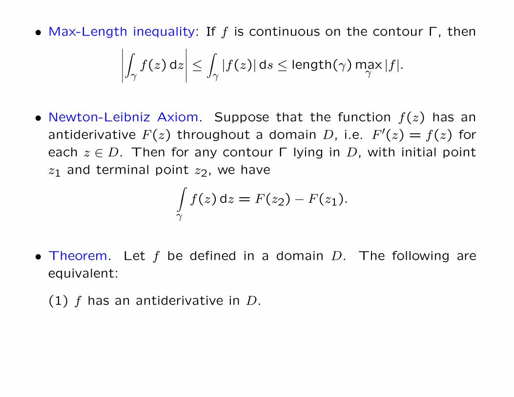
• Max-Length inequality: If f is continuous on the contour Γ, then∣∣∣∣∣∫γf(z) dz
∣∣∣∣∣ ≤∫γ|f(z)|ds ≤ length(γ) max
γ|f |.
• Newton-Leibniz Axiom. Suppose that the function f(z) has an
antiderivative F (z) throughout a domain D, i.e. F ′(z) = f(z) for
each z ∈ D. Then for any contour Γ lying in D, with initial point
z1 and terminal point z2, we have∫γ
f(z) dz = F (z2)− F (z1).
• Theorem. Let f be defined in a domain D. The following are
equivalent:
(1) f has an antiderivative in D.
(2) Every loop integral of f in D vanishes.
(3) The contour integrals of f are independent of path in D.
• Indefinite Integral. Suppose that f is continuous in a domain D
and the contour integrals of f are independent of path in D. Let
F (z) be the integral of f along some contour Γ in D joining z0
and z. Then F (z) is an antiderivative of f(z).

Cauchy’s Integral Theorem
• In this section, we always assume that D is a bounded domain
and its boundary ∂D is the union of finite closed contours.
The external boundary is always taken the positive orientation,
while the internal boundary is taken the negative oriented, so
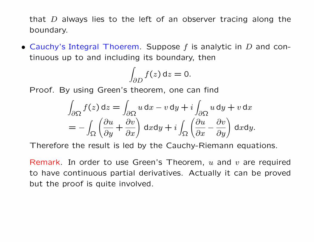
that D always lies to the left of an observer tracing along the
boundary.
• Cauchy’s Integral Thoerem. Suppose f is analytic in D and con-
tinuous up to and including its boundary, then∫∂D
f(z) dz = 0.
Proof. By using Green’s theorem, one can find∫∂Ω
f(z) dz =∫∂Ω
udx− v dy + i∫∂Ω
udy + v dx
= −∫
Ω
(∂u
∂y+∂v
∂x
)dxdy + i
∫Ω
(∂u
∂x−∂v
∂y
)dxdy.
Therefore the result is led by the Cauchy-Riemann equations.
Remark. In order to use Green’s Theorem, u and v are required
to have continuous partial derivatives. Actually it can be proved
but the proof is quite involved.
• A simply connected domain D is a domain having the following
property: If Γ is any simple closed contour lying in D, then the
domain interior to Γ lies wholly in D. Roughly speaking, a simply
connected domain has no hole inside.
• Corollary 1. Suppose that f is analytic in a simply connected
domain D and Γ is any loop in D, then∫Γ
f(z)dz = 0.
• Corollary 2. In a simply connected domain, an analytic function
has an antiderivative, its contour integrals are independent of
path, and its loop integrals vanish.

2.6 Cauchy’s Integral Formula and Its Consequences
• Cauchy’s Integral Formula. Suppose that z0 lies in an open do-
main D and f(z) is analytic in D and continuous up to and in-
cluding its boundary, then
f(z0) =1
2πi
∫∂D
f(z)
z − z0dz.
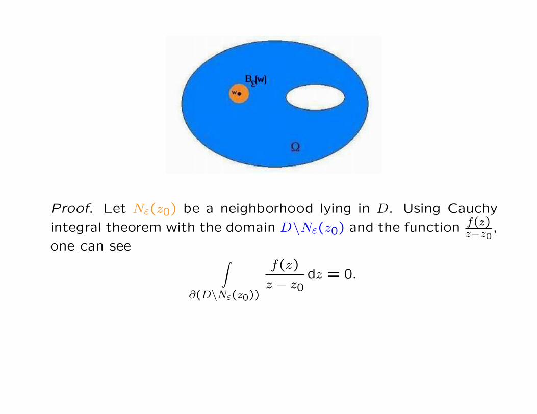
Proof. Let Nε(z0) be a neighborhood lying in D. Using Cauchy
integral theorem with the domain D\Nε(z0) and the function f(z)z−z0
,
one can see ∫∂(D\Nε(z0))
f(z)
z − z0dz = 0.
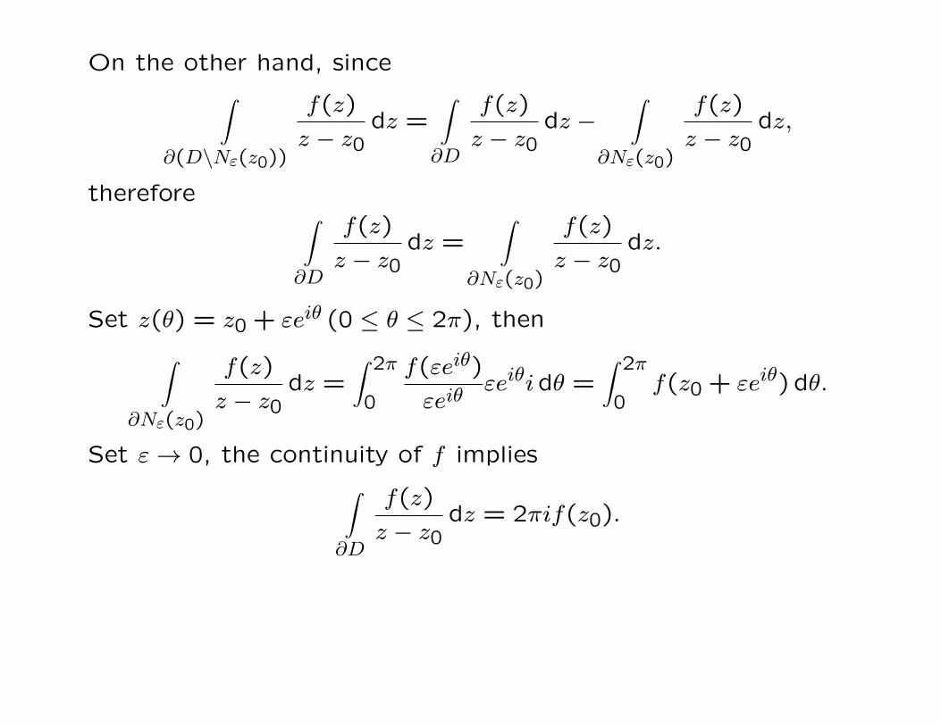
On the other hand, since∫∂(D\Nε(z0))
f(z)
z − z0dz =
∫∂D
f(z)
z − z0dz −
∫∂Nε(z0)
f(z)
z − z0dz,
therefore ∫∂D
f(z)
z − z0dz =
∫∂Nε(z0)
f(z)
z − z0dz.
Set z(θ) = z0 + εeiθ (0 ≤ θ ≤ 2π), then∫∂Nε(z0)
f(z)
z − z0dz =
∫ 2π
0
f(εeiθ)
εeiθεeiθidθ =
∫ 2π
0f(z0 + εeiθ) dθ.
Set ε→ 0, the continuity of f implies∫∂D
f(z)
z − z0dz = 2πif(z0).

• Higher Derivatives. Suppose that z0 lies in a open domain D
and f(z) is analytic in D and continuous up to and including its
boundary, then
f(n)(z0) =n!
2πi
∫∂D
f(z)
(z − z0)n+1dz.
Proof. It is led by differentiating both sides of Cauchy integral
formula with respect of z0.
• Morera’s Theorem. If f is continuous in a domain D and if each
loop integral of f in D vanishes, then f is analytic in D.
2.7 Taylor Series
• Geometric Series. The power series∞∑n=0
zn converges to 11−z if
|z| < 1.
• Comparison Test. Suppose that the terms cj satisfy the inequality|cj| ≤Mj for all integer j larger than some number J. Then if theseries
∑∞j=0Mj converges, so does
∑∞j=0 cj.
• Ratio Test. Suppose that the terms of the series∑∞j=0 cj have
the property that the ratios |cj+1/cj| approach a limit L as j →∞.Then the series converges if L < 1 and diverges if L > 1.
• Definition. The sequence Fn(z)∞n=1 is said to converge uniformlyto F (z) on the set T if for any ε > 0 there exists an integer Nsuch that when n > N ,
|F (z)− Fn(z)| < ε for all z in T .

• A power series is a series of the form∞∑n=0
an(z − z0)n, where an
and z0 are fixed complex numbers.
• For any power series∞∑n=0
an(z − z0)n, there exists R > 0 (may be
infinity), called the radius of convergence, such that
(1)the series converges in |z− z0| < R, and converges uniformlyin any closed subset of the disk.
(2)the series diverges in |z − z0| > R.
• The convergence radius can be computed by the formula
R =(
limn→∞
n√|an|
)−1=
(limn→∞
|an+1||an|
)−1
,
if the limit exist. In general,
R =(
limn→∞
n√|an|
)−1.

• The convergence is uniform and absolute in every closed disc in
D, that is to say the series can be differentiated and integrated
termwise in D.
• A power series∞∑n=0
an(z − z0)n is analytic in the convergence do-
main.
• If f is analytic in Dr = |z − z0| < r, then for all z ∈ Dr, f can be
uniquely expressed as the following series:
f(z) =∞∑n=0
an(z − z0)n,
where an = f(n)(z0)n! . Such series is called Taylor series of f around
z0. Furthermore, the convergence of the series is uniform in any
closed subset of Dr.

Proof. For fixed positive ρ < r, by Cauchy integral formula,
f(z) =1
2πi
∫|w−z0|=ρ
f(w)
w − zdw =
1
2πi
∫|w−z0|=ρ
f(w)
(w − z0)(1− z−z0w−z0
)dw.
Noting that | z−z0w−z0
| < 1, using the lemma above, integrating termby term and using the formula for higher derivatives, we have
f(z) =1
2πi
∫|w−z0|=ρ
f(w)
w − z0
∞∑n=0
(z − z0
w − z0
)ndw
=∞∑n=0
1
2πi
∫|w−z0|=ρ
f(w)
(w − z0)n+1dw
(z − z0)n
=∞∑n=0
f(n)(z0)
n!(z − z0)n.
The uniqueness is following by differentiating both sides and valu-ing at z0.

• Remark. The theorem implies that the Taylor series will convergeto f(z) everywhere inside the largest open disk, centered at z0,over which f is analytic.
• Taylor series of some elementary functions.
ez =∞∑n=0
zn
n!= 1 + z +
z2
2!+z3
3!+ · · · , z ∈ C,
cos z =∞∑n=0
(−1)n
(2n)!z2n = 1−
z2
2!+z4
4!+ · · · , z ∈ C,
sin z =∞∑n=0
(−1)n+1
(2n+ 1)!z2n+1 = z −
z3
3!+z5
5!+ · · · , z ∈ C,
log(1− z) = −∞∑n=1
zn
n= −z −
z2
2−z3
3− · · · , |z| < 1.
• Again this is a remarkable property which is not shared by func-tions of real variables. A function need not have a convergent

Taylor series expansion even if it is infinitely differentiable. For
example,
f(x) =
e− 1x2 , x > 0,
0, x ≤ 0.
• Theorem. If f is analytic at z0, the Taylor series for f ′ around z0
can be obtained by termwise differentiation of the Taylor series
for f around z0 and converges in the same disk as the series for
f .
• Historically, we call a function f(z) is analytic at z0 if f(z) can be
locally expressed as a power series
f(z) =∞∑n=0
an(z − z0)n
around z0. We now see analyticity is equivalent to differentiability.

Chapter 3
Isolated Singularities

3.1 Zeros and Singularities
• Zeros. A point z0 is called a zero of order m for the analytic
function f if f and its first m − 1 derivatives vanish at z0, but
f(m)(z0) 6= 0.
• Assume that z0 is a zero of order m of the analytic function f(z),
then the Taylor series for f around z0 takes the form
f(z) =∞∑n=k
an(z − z0)n = (z − z0)k∞∑n=0
an+k(z − z0)n,
which implies the following proposition.
Proposition. If z0 is a zero for the analytic function f(z), then
either f is identically zero in a neighborhood of z0 or there is a
punctured disk about z0 in which f has no zeros.
By using the connectivity of D, we can obtain a stronger theorem.
Theorem. If f is analytic in a domain D and z0 is a zero for f ,
then either f is identically zero in D or there is a punctured disk
about z0 in which f has no zeros.
That is to say the zeros for a nonconstant analytic function must
be isolated.
Corollary If f(z) and g(z) are analytic in D and f(z) = g(z) on a
set which has an accumulation point in D, then f(z) identically
equals to g(z).
• Singularity. A point is called a singularity of f(z), if f(z) fails to
be analytic at this point.
• A singularity z0 of f(z) is called isolated, if f(z) is analytic in some
annulus 0 < |z − z0| < ε.

Example 1 0 is a isolated singularity of sin zz , 1
z or sin 1z .
Example 2 0 is a singularity of log z, but not isolated.

3.2 Laurent Series
• If f is analytic in the annulus D = r < |z−z0| < R, then for each
z ∈ D
f(z) =+∞∑
n=−∞cn(z − z0)n,
where the coefficients are given by
cn =1
2πi
∫γ
f(w)
(w − z0)n+1dz
and γ is any simply closed curve lying in D containing z0 in its
interior. This series is called Laurent series of f in the annulus D.
Moreover such a series expansion is unique.
Proof. For any z ∈ D, take ε > 0 such that z ∈ Ω = r − ε <|z − z0| < R − ε. Since f is analytic in Ω and continuous in Ω,

using Cauchy integral formula, we find
f(z) =1
2πi
∫∂Ω
f(w)
w − zdw =
1
2πi
∫|w−z0|=R+ε
f(w)
w − zdw −
1
2πi
∫|w−z0|=r−ε
f(w)
w − zdw.

Noting that the following series hold for z ∈ Ω
1
w − z=
1
w − z0·
1
1− z−z0w−z0
=∞∑n=0
(z − z0)n
(w − z0)n+1, for |w − z0| = R− ε,
−1
w − z=
1
z − z0·
1
1− w−z0z−z0
=∞∑n=1
(w − z0)n−1
(z − z0)n, for |w − z0| = r + ε,
the integral above can be rewritten as∫|w−z0|=R+ε
f(w)
w − zdw =
∞∑n=0
(z − z0)n∫
|w−z0|=R+ε
f(w)
(w − z0)n+1dw,
−∫
|w−z0|=r−ε
f(w)
w − zdw =
∞∑n=1
(z − z0)−n∫
|w−z0|=r−ε
f(w)(w − z0)n−1 dw.

Set
cn =
1
2πi
∫|w−z0|=R+ε
f(w)
(w − z0)n+1dw, for n ≥ 0,
1
2πi
∫|w−z0|=r−ε
f(w)
(w − z0)n+1dw, for n < 0,
one can see
f(z) =+∞∑
n=−∞cn(z − z0)n.
Furthermore for any simple closed curve γ ⊂ Ω, by Cauchy integral
theorem, we have∫|w−z0|=R+ε
f(w)
(w − z0)n+1dw =
∫|w−z0|=r−ε
f(w)
(w − z0)n+1dw =
∫γ
f(w)
(w − z0)n+1dw.
The uniqueness follows by dividing both sides of series by (z −

z0)n+1 and integrating along γ.
• Remark 1 The Laurent series of f depends on not only the center
point z0 but the annulus D, while the Taylor series only depends
on the center point.
• Remark 2 It is usually very hard to compute the coefficients in
Laurent series by integral. However we can use the formulae
for Taylor series to get the coefficients in Laurent series, and it
also gives us another way to compute the integrals. One of the
significant results is residue theorem, which will be shown in the
next chapter.
3.3 Three Types of Isolated Singularities
• Definition. If z0 is an isolated singularity of f(z), then f(z) has a
Laurent expansion as
f(z) =+∞∑
n=−∞cn(z − z0)k
in a punctured disc 0 < |z − z0| < ε. We classify the isolated
singularities into three categories.
(1) If aj = 0 for all j < 0, we say that z0 is a removable singularity.
(2) If a−m 6= 0 for some positive integer m but aj = 0 for all
j < −m, we say that z0 is a pole of order m.
(3) If aj 6= 0 for an infinite number of negative values of j, we say
that z0 is an essential singularity of f .

• Behavior near the isolated singularity. Let z0 be an isolated sin-gularity of f(z).
(1) z0 is removable iff limz→z0
f(z) exists finite.
(2) z0 is a pole iff limz→z0
f(z) =∞.
(3) z0 is an essential singularity iff limz→z0
f(z) does not exist.
• Theorem Let z0 be an isolated singularity of f(z).
(1) z0 is removable iff f(z) is bounded in a punctured neighbor-hood of z0.
(2) z0 is a pole of order m iff limz→z0
(z − z0)lf(z) =∞ for all l < m,
while (z − z0)mf(z) has a removable singularity at z0.
• Picard’s Theorem Let z0 be an essential singularity of f(z) and U
be any punctured neighborhood of z0, then for any w ∈ C, except

perhaps one value, the equation f(z) = w has infinitely manysolutions in U .
That is to say that an analytic function assumes every complexnumber, with possibly one exception, as a value in any puncturedneighborhood of an essential singularity.
• ∞ as a Singularity If there exist some R > 0 such that f(z) isanalytic in the domain |z| > R, then ∞ is also called an isolatedsingularity of f(z).
∞ is called a removable singularity, pole or essential singularity off(z) respectively , if 0 is a removable singularity, pole or essentialsingularity of f(1
z).
• Meromorphic Function A function f(z) which is analytic in D
except for removable singularities and poles, is said to be mero-morphic in D. That is to say a meromorphic function has noessential singularity.

A meromorphic function in D can be regarded as a mapping from
D to Riemann sphere.
Theorem f(z) is a meromorphic function in the extended complex
plane C iff f(z) is a rational function.
3.4 The Residue Theorem
• Definition. If f has an isolated singularity at the point z0, thenthe coefficient c−1 of (z − z0)−1 in the Laurent expansion for faround z0 is called the residue of f(z) at z0 and is denoted byRes(f, z0).
• If f(z) has a removable singularity at z0, Res(f, z0) = 0.
If f(z) = g(z)h(z) where g(z), h(z) are analytic at z0, g(z0) 6= 0, h(z0) =
0 and h′(z0) 6= 0, then z0 is a simple pole of f(z) and
Res(f, z0) =g(z0)
h′(z0).
If f(z) has a pole of order k at z0, then
Res(f, z0) =1
(k − 1)!limz→z0
dk−1
dzk−1[(z − z0)kf(z)].

• The residue plays an important role in the contour integration.If Γ is a simple closed positively oriented contour and f(z) isanalytic on and inside Γ except for a single isolated singularity z0
lying interior to Γ, then the integral∫Γ
f(z)dz = 2πiRes(f, z0).
In general, we have
Cauchy’s Residue Theorem. If Γ is a simple closed positivelyoriented contour and f(z) is analytic on and inside Γ except atthe points z1, . . . , zn inside Γ, then the integral∫
Γ
f(z)dz = 2πin∑
j=1
Res(f, zj).
Proof. Let D be the interior of Γ and take the disjoint neighbor-hood Bε(z1), Bε(z2), . . . , Bε(zn) in D like the figure,

and set Ω = D \n⋃
k=1
Bε(zk), then
∫Γ
f(z) dz =∫∂Ω
f(z) dz +n∑
k=1
∫∂Bε(zk)
f(z) dz = 2πin∑
k=1
Res (f, zk).
• Residue at ∞. If ∞ is an isolated singularity of f(z), i.e. thereexists R > 0 such that f(z) is analytic in the annulus R < |z| <
∞, then the residue of f(z) at ∞ is defined by
Res(f(z),∞) = −1
2πi
∫|z|=R
f(z)dz.
Remark. We take the minus sign in the definition, since ∞ lies
outside the circle |z| = R.
If we set w = 1z then
Res(f(z),∞) = −1
2πi
∫|z|=R
f(z)dz =1
2πi
∫|w|= 1
R
f(1
w)
1
w2dw = Res(f(
1
w)
1
w2,0).
• Theorem. If f(z) has finite isolated singularities in the extend-
ed complex plane C, the sum of the residues of all the isolated
singularities must be zero.

3.5 The Applications of Residue Theorem
1. Trigonometric Integrals over [0,2π]
• The real integrals of the form∫ 2π
0R(cos θ, sin θ)dθ
can be evaluated by the residue theorem, where R(cos θ, sin θ) is
a rational function (with the real coefficients) of cos θ, sin θ and is
finite over [0,2π].
• If we parametrize the unit circle by z = eiθ (0 ≤ θ ≤ 2π), we have
the identities
cos θ =1
2
(z +
1
z
), sin θ =
1
2i
(z −
1
z
), dz = ieiθdθ.

Therefore∫ 2π
0R(cos θ, sin θ)dθ =
∫|z0|=1
[1
izR
(1
2
(z +
1
z
),
1
2i
(z −
1
z
))]dz.

2. Improper Integrals of Certain Functions over (−∞,+∞)
If P (x), Q(x) are polynomials satisfying
degP (x) ≤ degQ(x)− 2,
and Q(x) has no real zero on (−∞,+∞), then
+∞∫−∞
P (x)
Q(x)dx = 2πi
∑Im z0>0
Res
P (z)
Q(z), z0
.

3. Improper Integrals Involving Trigonometric Functions
If P (x), Q(x) are polynomials satisfying
degP (x) ≤ degQ(x)− 1,
and Q(x) has no zero on (−∞,+∞), then
+∞∫−∞
P (x)
Q(x)cosαxdx = Re
2πi∑
Im z0>0
Res
(P (z)
Q(z)ei|α|z, z0
) ,+∞∫−∞
P (x)
Q(x)sinαxdx = sgn(α)Im
2πi∑
Im z0>0
Res
(P (z)
Q(z)ei|α|z, z0
) .

Chapter 4
The Applications of Analytic
Functions

4.1 Harmonic Functions
• Definition. A real valued function u(x1, . . . , xn) of n real variables
are called harmonic in D if u satisfies Laplace equation
4u def=
∂2u
∂x21
+∂2u
∂x21
+ · · ·+∂2u
∂x2n
= 0
at each point of D.
Remark. (x1, . . . , xn) must be the euclidean coordinate.
• Proposition. If f(z) is analytic in D, then both the real part u(x, y)
and the imaginary part v(x, y) are harmonic in D.
• Given a function u(x, y) harmonic in an open disk D, then we can
find another harmonic function v(x, y) so that u+ iv is analytic in
D. Such a function v is called a harmonic conjugate of u.

4.2 Bounds of Analytic Functions
• The Mean Value Property. Let f be analytic in a domain D andthe disc |z − z0| ≤ r be contained in D. Therefore
f(z0) =1
2π
2π∫0
f(z0 + reiθ)dθ.
• The Maximum Modulus Principle. If f(z) is analytic and non-constant in a domain D, then |f(z)| cannot achieve its maximumvalue in D.
• Cauchy inequalities. Let f(z) be analytic in a domain D and|f(z)| ≤ M for all z in the disc |z − z0| ≤ r contained in D.Therefore for any nonnegative integer n,
|f(n)(z0)| ≤n!M
rn.

The proof can be obtained by using the inequality of integral.
• Liouville Theorem. The only bounded entire functions are theconstant function.
Proof. Assume that |f(z)| ≤ M for any z ∈ C, then by Cauchyinequalities
|f ′(z)| ≤M
r
for any z and positive r. Setting r → +∞, we obtain f ′(z) = 0which leads to the conclusion.
• The Fundamental Theorem of Algebra. Every nonconstant poly-nomial with complex coefficients has at least one zero.
• Picard Theorem. Let f(z) be an entire nonconstant function, thenfor any w ∈ C, except perhaps one value, the equation f(z) = w
has at least one solution in C.

Applications to Harmonic Functions
• Theorem. Let u(x, y) be a harmonic function in a simply connect-
ed domain D. Then there exist another harmonic function v(x, y)
so that f(z) = u+ iv is analytic in D. Moreover v is unique up to
addition a constant.
• The Mean Value Property. Let u be harmonic in a domain D and
the disc |z − z0| ≤ r be contained in D. Therefore
u(x0, y0) =1
2π
2π∫0
u(x0 + r cos θ, y0 + r sin θ)dθ.
• The Maximum Principle. If u(x, y) is harmonic and nonconstant
in a domain D, then u(x, y) can achieve neither maximum nor
minimum in D.

• Liouville Theorem. If u(x, y) is a bounded harmonic function in
R2, then u(x, y) must be a constant.

Chapter 5
Conformal Mappings
5.1 Geometric Considerations
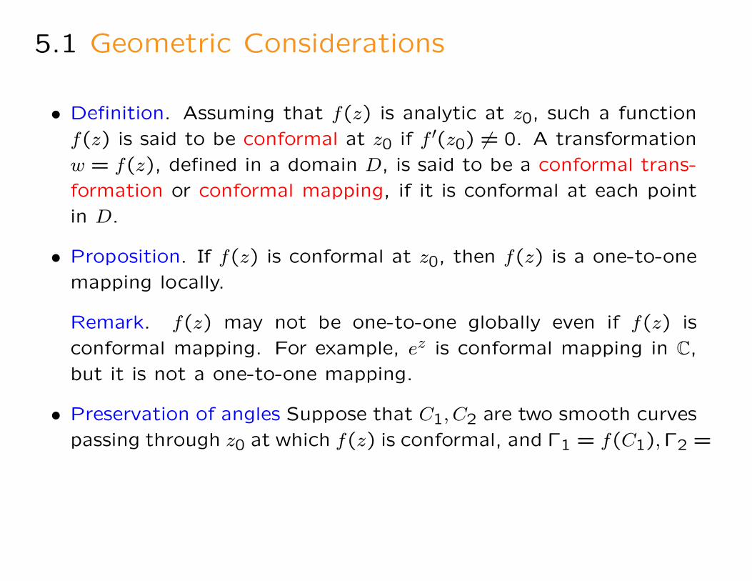
• Definition. Assuming that f(z) is analytic at z0, such a function
f(z) is said to be conformal at z0 if f ′(z0) 6= 0. A transformation
w = f(z), defined in a domain D, is said to be a conformal trans-
formation or conformal mapping, if it is conformal at each point
in D.
• Proposition. If f(z) is conformal at z0, then f(z) is a one-to-one
mapping locally.
Remark. f(z) may not be one-to-one globally even if f(z) is
conformal mapping. For example, ez is conformal mapping in C,
but it is not a one-to-one mapping.
• Preservation of angles Suppose that C1, C2 are two smooth curves
passing through z0 at which f(z) is conformal, and Γ1 = f(C1),Γ2 =

f(C2) are the image curves, then the angle from Γ1 to Γ2 is the
same as the angle from C1 to C2, in sense as well as in size.
arg f(z0) is the rotation angle.
• Scale factors Any small line segment with one end point at z0,
where f(z) is conformal, is contracted or expanded in the ratio
|f ′(z0)| by the mapping.
• The Open Mapping Property. If f is nonconstant and analytic in
a domain D, then its range f(D) is an open set.

• Riemann Mapping Theorem. Let D be any simply connected
domain in the plane other than the entire plane itself. Then there
exists a one-to-one analytic function that maps D onto the open
unit disk. Moreover, one can prescribe an arbitrary point of D
and a direction through that point which are to be mapped to
the origin and the direction of the positive real axis, respectively.
Under such restrictions the mapping is unique.
Remark. The Riemann mapping theorem is an existence theorem.
The precise expression of the Riemann mapping can only be found
for some special domains.

5.2 Mobius Transformations
• Definition. The transformation
f(z) =az + b
cz + d(a, b, c, d ∈ C, ad− bc 6= 0)
is called a fractional linear transformation or Mobius transforma-tion.
Proposition. A composition of two Mobius transformations is aMobius transform. An inverse transform of a Mobius transform isa Mobius transform.
Proposition. A Mobius transformation can be regarded as a one-to-one conformal mapping to the extended complex plane ontoitself.
Proposition. A Mobius transformation can be written by thecomposition of three special transformations: (1) Translation
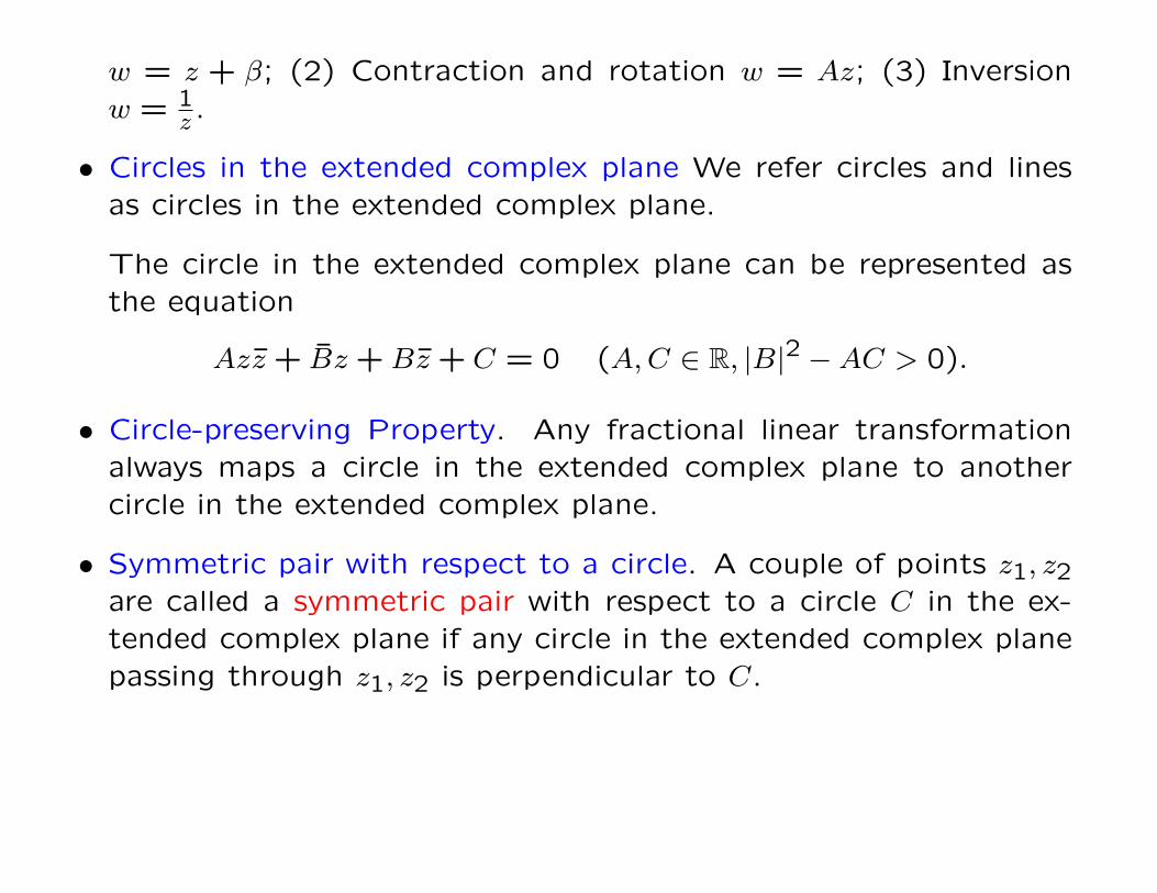
w = z + β; (2) Contraction and rotation w = Az; (3) Inversionw = 1
z .
• Circles in the extended complex plane We refer circles and linesas circles in the extended complex plane.
The circle in the extended complex plane can be represented asthe equation
Azz + Bz +Bz + C = 0 (A,C ∈ R, |B|2 −AC > 0).
• Circle-preserving Property. Any fractional linear transformationalways maps a circle in the extended complex plane to anothercircle in the extended complex plane.
• Symmetric pair with respect to a circle. A couple of points z1, z2are called a symmetric pair with respect to a circle C in the ex-tended complex plane if any circle in the extended complex planepassing through z1, z2 is perpendicular to C.
Proposition Suppose that z1, z2 is a symmetric pair with respect
to a circle C in the extended complex plane and f(z) is a Mobius
transformation, then f(z1), f(z2) is a symmetric pair with respect
to f(C).

5.3 Mobius Transformations, Continued
• Mapping the upper half plane onto the unit disc w = eiθz−λz−λ.
• Mapping the unit disc onto the unit disc w = eiθ z−α1−αz.
• Mapping (z1, z2, z3) to (w1, w2, w3) z−z1z−z2
: z3−z1z3−z2
= w−w1w−w2
: w3−w1w3−w2
.
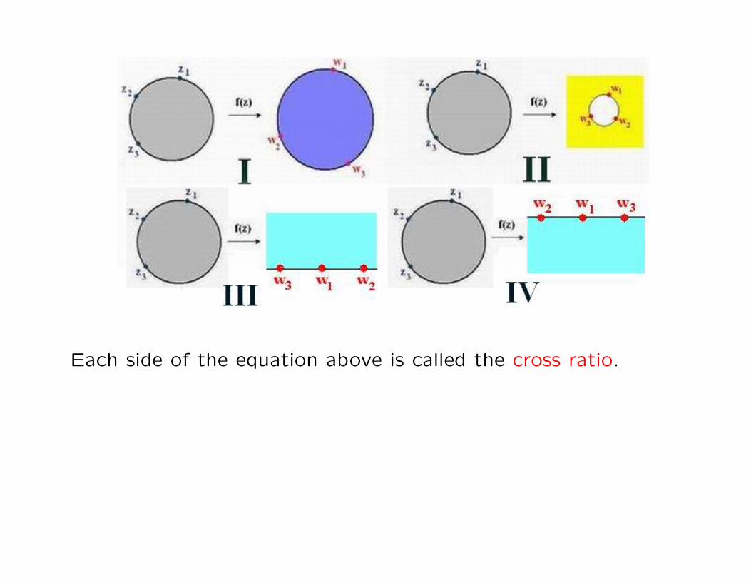
Each side of the equation above is called the cross ratio.
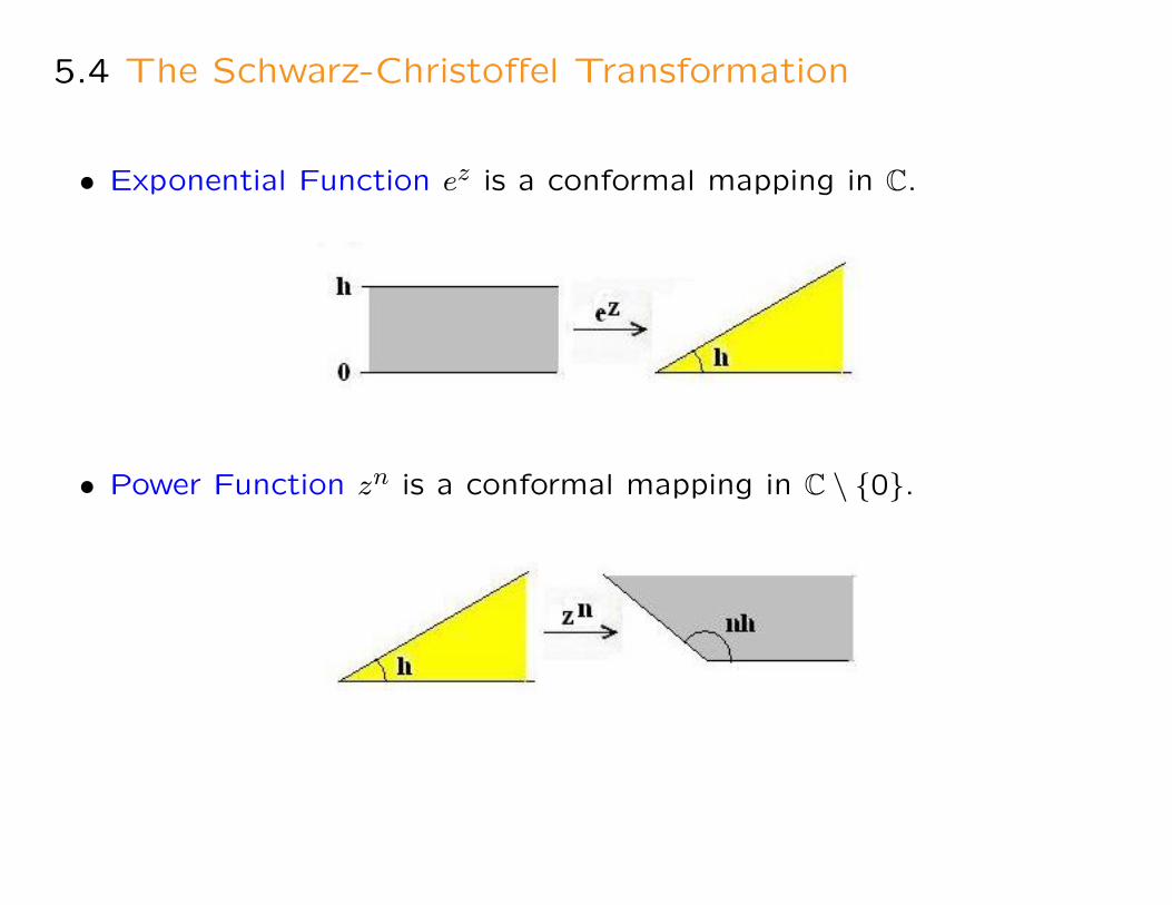
5.4 The Schwarz-Christoffel Transformation
• Exponential Function ez is a conformal mapping in C.
• Power Function zn is a conformal mapping in C \ 0.

Chapter 6
The Transforms of Applied
Mathematics
6.1 The Fourier Transform
• Definition If f(x) is defined for all real x, then the integral
+∞∫−∞
f(x)e−iωxdx (1)
is called Fourier transform of f(x), denoted as f(ω) or F [f(x)].
The principle value of the integral
1
2πlim
N→+∞
N∫−N
f(ω)eiωxdω (2)
is called inverse Fourier transform of f(ω), denoted by F−1[f(ω)].
• Remark The integral (1) converges for all f ∈ L1(R), where
L1(R) = f :∫R |f |dx < +∞. Otherwise (1) may diverge.
• Fourier Inversion Formula. If f ∈ L1(R) is continuous except fora finite number of jumps, then
limN→+∞
1
2π
N∫−N
f(ω)eiωxdω =1
2(f(x+ 0) + f(x− 0)),
where f(x+ 0), f(x− 0) denote the left and right limits of f at x.
• Corollary For any f ∈ L1(R) ∩ C(R), f = F−1(F(f)), where C(Ris the set of all the continuous functions defined in R
• The Properties of Fourier Transform
1. Linearity F(l1f1 + l2f2) = l1F(f1) + l2F(f2).
2. Translation For any x0 ∈ R, F(f(x− x0)) = e−iωx0f(ω).
3. Scaling For any nonzero k ∈ R, F(f(kx)) = 1|k|f(ωk).
4. Duality If f ∈ L1(R) ∩ C(R) and h(ω) = (f(x)), then h(ω) =2πf(−ω).

5. Convolution Define the convolution of f1, f2 as f1 ∗ f2(x) =+∞∫−∞
f1(x− y)f2(y) dy, then F(f1 ∗ f2) = F(f1)F(f2).
6. Differentiation If f, f ′ ∈ L1(R), then F(f ′(x)) = iωF(f(x)).
7. Integration F(x∫0f(τ) dτ) = 1
iωF(f).
6.2 The Laplace Transform
• Definition If f(t) is defined for t > 0, and the integral∫ ∞0
f(t)e−stdt (3)
exists for some s, then the integral (3) is called Laplace transform
of f(t), denoted as F (s) or L [f(t)].
• Theorem (i) If the integral (3) converges for some real β, then (3)
converges whenever Re s > β, and F (s) is analytic in Re s > β.
(ii) If the integral (3) diverges for some real β, then (3) diverges
whenever Re s < β.
• The Properties of Laplace Transform
1. Linearity L (l1f1 + l2f2) = l1L (f1) + l2L (f2).

2. Time scaling For any positive k, L (f(kt)) = 1kL (f)(sk).
3. Time shifting If f(t) = 0 holds for any negative t, then for any
a > 0, L (f(t− a)) = e−asL (f)(s).
4. Frequency shifting L (eatf(t)) = L (f)(s− a).
5. Convolution Define the convolution of f1, f2 as f1 ∗ f2(t) =t∫
0f1(t− τ)f2(τ) dτ, then L (f1 ∗ f2) = L (f1)L (f2).
6. Differentiation L (f(n)(t)) = snL (f)−sn−1f(0)−· · ·−f(n−1)(0).
7. Integration L (t∫
0f(τ) dτ) = 1
sL (f).
• Theorem. For any rational function F (s) = P (s)Q(s) satisfying degP (s) <
degQ(s), there exists a unique continuous function f(t) such that
L (f(t)) = F (s), which is called inverse Laplace transform of F (s),
denoted by L−1(F (s)).
Proof. Since any rational function F (s) = P (s)Q(s), satisfying degP (s) <
degQ(s), has a partial fraction decomposition
F (s) =m∑j=1
n∑k=1
Cjk
(s− sj)k,
we can set
f(t) =m∑j=1
n∑k=1
tk−1esjt.
• We can use Laplace transform to solve linear ODEs (ordinary
differential equations).