fundamental studies in the lamb-wave interaction between
TRANSCRIPT

FUNDAMENTAL STUDIES IN THE LAMB-WAVE INTERACTION
BETWEEN PIEZOELECTRIC WAFER ACTIVE SENSOR AND HOST
STRUCTURE DURING STRUCTURAL HEALTH MONITORING
by
Giola Santoni
Bachelor of Science
University of Pisa, Pisa, Italy, 1999
Submitted in Partial Fulfillment of the Requirements
For the Degree of Doctor of Philosophy
Mechanical Engineering
College of Engineering and Information Technology
University of South Carolina
2010
Accepted by:
Victor Giurgiutiu, Major Professor
Sarah Baxter, Committee Member
Yuh Chao, Committee Member
Sarah Gassman, Committee Member
ii
ACKNOWLEDGMENTS
The author is grateful to many to accomplish this goal. The author would like to
expresses her sincere gratitude for her advisor, Prof. Victor Giurgiutiu, for his continuous
support, encouragement, motivation and guidance throughout all phases of her Ph.D.
study. The author would like to thank her defense committee members, Prof. Sarah
Baxter, Prof. Yuh Chao, Prof. Sarah Gassman, for their comments, suggestions and time
for reviewing this work. The author is thankful to former graduate director Prof. Xiaomin
Deng and current graduate director Prof. Tony Reynolds for their countless helps during
the years.
The author would like to thank LAMSS research group members: Lucy Yu, Bin Lin,
Buli Xu, Tom Behling, Patrick Pollock, Weiping Liu, Adrian Cuc, James Kendall, Greg
Crachiolo, for their invaluable suggestions, comments, and friendship.
The author wishes to dedicate this dissertation to her husband for his continuous
support, patience and understanding and to her children for being so nice and for thinking
that her work consists in making toys.

iii
ABSTRACT
The scope of my research was to develop a better understanding of the engineering
variables that influence the interaction of PWAS with structure during activation of the
transducer. This is a key feature needed to develop more power/energy efficient structural
health monitoring (SHM) systems. SHM is the field of engineering that determines the
health of a structure while it is in service. Active SHM can be performed through
piezoelectric transducers such as piezoelectric wafer active sensors (PWAS) that can be
permanently attached to the structure through a bonding layer. PWAS transducers can
actively interrogate the structure by exciting and receiving Lamb waves propagating in
the structure or by passively listen to changes in the structure. PWAS-structure
interaction modeling is fundamental in order to achieve single mode excitation, i.e.,
tuning, a requirement for most of the SHM algorithms (time reversal, phase-array, and
imaging).
To achieve our research goal, we had to go beyond the current state of the art in
modeling and understanding the load transfer from PWAS to the structure. The existing
modeling methods rely on the low frequency assumption of axial/flexural waves only.
This assumption is not true in the high frequency range of ultrasonic SHM applications.
We derived, through the normal mode expansion methods (NME), the interfacial shear
stress, hence, the load transfer from the PWAS to the structure through the bond layer,
without limitations on the frequency and the number of modes. This allowed us to derive

iv
more accurate predictions of the tuning between PWAS and Lamb waves which
compared very well with experimental measurements.
This dissertation is constructed in three major parts.
In Part I, we developed a generic formulation for ultrasonic guided waves in thin wall
structures. The formulation is generic because, unlike many authors, in many parts of our
derivation (power flow, reciprocity theorem, orthogonality, etc.) we stayed away from
specifying the actual mathematical expressions of the guided wave modes and maintained
a generic formulation throughout.
In Part II, we addressed some unresolved issues of the PWAS SHM predictive
modeling. We extended the NME theory to the case of PWAS bonded to or embedded in
the structure. We developed the shear layer coupling between PWAS and structure using
N generic guided wave modes and solving the resulting integro-differential equation for
shear lag transfer. We applied these results to predicting the tuning between guided
waves and PWAS and obtained excellent agreement with experimental results.
Another novel aspect covered in this dissertation is that of guided waves in composite
materials. The increasing use of composites in aeronautical and space applications makes
it important to extend SHM theory to such materials. For this reason, the NME theory is
extended to the case of composites. We developed a generic formulation for the tuning
curves that was not directly dependent on the composite layup and can be easily extended
to various composite formulations. We conducted carefully-planned experiments on
composites with different orientations. The comparison between our predictions and
experiments was quite good.

v
In Part III, SHM applications and related issues are addressed. We discussed the
reliability of SHM systems and the lack of specifications for quality SHM inspections
with particular focus on the case of composites SHM. We determined experimentally the
ability of PWAS to detect damage in various composite specimens. We tested the
performance of the PWAS for damage detection on composite plates, on unidirectional
composite strips, on quasi-isotropic plates, on lap-joints junctions, and composite tank
sections. We also tested the ability of PWAS transducers to operate under extreme
environments and high stress conditions, i.e. the survivability of PWAS-based SHM. We
proved the durability of the entire PWAS-based SHM system under various different load
conditions. We also tested the influence of bond degradation on PWAS electrical
capacitance as installed on the structure, which gives a measure of the quality of the
PWAS installation, a key feature in PWAS-based SHM. We developed theoretical
models for shear horizontal waves scattering from a crack and Lamb waves scattering
from change in material properties. We studied the acoustic emission (AE) in infinite
plate and we used NME to model AE phenomena.

vi
TABLE OF CONTENTS
ACKNOWLEDGMENTS............................................................................................................................II
ABSTRACT ................................................................................................................................................ III
LIST OF TABLES ..................................................................................................................................... XI
LIST OF FIGURES ................................................................................................................................ XIII
1 INTRODUCTION..................................................................................................................................1
1.1 MOTIVATION.................................................................................................................................1
1.2 RESEARCH GOAL, SCOPE, AND OBJECTIVES ...................................................................................3
1.3 DISSERTATION LAYOUT ................................................................................................................5
PART I ELASTIC WAVES FOR STRUCTURAL HEALTH MONITORING .................................9
2 ACOUSTIC FIELD EQUATIONS.....................................................................................................12
2.1 EQUATION OF MOTION ................................................................................................................12
2.2 STRAIN-DISPLACEMENT EQUATION .............................................................................................15
2.3 HOOKE’S LAW.............................................................................................................................16
2.4 ACOUSTIC FIELD EQUATIONS SUMMARY .....................................................................................17
3 GUIDED WAVES IN PLATES ..........................................................................................................18
3.1 STRAIGHT-CRESTED GUIDED WAVES IN RECTANGULAR COORDINATES .......................................18
3.2 CIRCULAR-CRESTED GUIDED WAVES IN CYLINDRICAL COORDINATES .........................................37
4 POWER FLOW AND ENERGY CONSERVATION – THE ACOUSTIC POYNTING
THEOREM..................................................................................................................................................61
4.1 POWER FLOW IN RECTANGULAR COORDINATES ..........................................................................67

vii
4.2 POWER FLOW IN CYLINDRICAL COORDINATES.............................................................................90
5 RECIPROCITY RELATION ...........................................................................................................113
5.1 REAL RECIPROCITY RELATION...................................................................................................115
5.2 COMPLEX RECIPROCITY RELATION............................................................................................117
5.3 REAL RECIPROCITY RELATION IN RECTANGULAR COORDINATES...............................................122
5.4 COMPLEX RECIPROCITY RELATION IN RECTANGULAR COORDINATES........................................126
5.5 REAL RECIPROCITY RELATION IN CYLINDRICAL COORDINATES.................................................129
5.6 COMPLEX RECIPROCITY RELATION IN CYLINDRICAL COORDINATES ..........................................133
6 ORTHOGONALITY RELATION...................................................................................................137
6.1 ORTHOGONALITY RELATION WITHOUT ASSUMPTIONS ON THE SOLUTION..................................137
6.2 ORTHOGONALITY RELATION IN RECTANGULAR COORDINATES .................................................157
6.3 ORTHOGONALITY RELATION IN CYLINDRICAL COORDINATES ...................................................167
PART II PWAS-BASED STRUCTURAL HEALTH MONITORING .............................................174
7 PWAS EXCITATION OF GUIDED WAVES.................................................................................177
7.1 PIEZOELECTRIC WAFER ACTIVE SENSORS CHARACTERISTICS ....................................................177
7.2 PWAS EXCITATION OF STRAIGHT-CRESTED GUIDED WAVES.....................................................182
7.3 PWAS EXCITATION OF CIRCULAR-CRESTED GUIDED WAVES ....................................................191
7.4 NORMAL MODE EXPANSION MODEL WITH SURFACES FORCES....................................................197
7.5 NORMAL MODE EXPANSION MODEL WITH VOLUME FORCES .....................................................210
8 SHEAR LAYER COUPLING BETWEEN PWAS AND STRUCTURE......................................213
8.1 PROBLEM DEFINITION ...............................................................................................................215
8.2 SHEAR-LAG SOLUTION FOR AXIAL AND FLEXURAL MODES........................................................217
8.3 SHEAR-LAG SOLUTION FOR TWO MODES, ONE SYMMETRIC AND THE OTHER ANTISYMMETRIC ..232
8.4 SHEAR-LAG SOLUTION FOR N GENERIC MODES ......................................................................238
8.5 STRESS DISTRIBUTION IN THE BONDING LAYER .........................................................................260

viii
9 TUNED GUIDED WAVES EXCITED BY PWAS .........................................................................264
9.1 SHEAR TRANSFER THROUGH BOND LAYER ................................................................................265
9.2 PWAS – LAMB WAVES TUNING ................................................................................................271
10 TUNED GUIDED WAVES IN COMPOSITE PLATES ................................................................288
10.1 DISPERSION CURVES IN COMPOSITE PLATES ..............................................................................289
10.2 PWAS – GUIDED WAVES TUNING..............................................................................................313
PART III STRUCTURAL HEALTH MONITORING ISSUES AND APPLICATIONS .................326
11 RELIABILITY OF STRUCTURAL HEALTH MONITORING..................................................329
11.1 SPECIFICATIONS FOR QUALITY STRUCTURAL HEALTH MONITORING INSPECTION ......................329
11.2 PROBABILITY OF DETECTION CURVES .......................................................................................333
12 SPACE QUALIFIED NON-DESTRUCTIVE EVALUATION & STRUCTURAL HEALTH
MONITORING .........................................................................................................................................340
12.1 INTRODUCTION .........................................................................................................................340
12.2 SUBSYSTEM/COMPONENT SPECIFICATION .................................................................................341
12.3 DAMAGE DETECTION EXPERIMENTS ON TEST SPECIMENS..........................................................347
13 SURVIVABILITY OF SHM SYSTEMS .........................................................................................362
13.1 TEST SPECIFICATIONS................................................................................................................362
13.2 TEST PROCEDURE......................................................................................................................363
13.3 RESULTS ...................................................................................................................................365
13.4 CONCLUSION.............................................................................................................................373
14 DURABILITY OF SHM SYSTEMS ................................................................................................374
14.1 REQUIREMENTS.........................................................................................................................374
14.2 MISSION PROFILE ......................................................................................................................375
14.3 SHOCK TEST..............................................................................................................................377
14.4 RANDOM VIBRATION TEST .......................................................................................................379

ix
14.5 THERMAL TEST .........................................................................................................................379
14.6 ACOUSTIC ENVIRONMENT TEST.................................................................................................380
15 EFFECT OF PARTIAL BONDING BETWEEN TRANSDUCER AND STRUCTURE ON
CAPACITANCE .......................................................................................................................................381
15.1 POWER ANALYSIS AND SAMPLE SIZE .........................................................................................383
15.2 POPULATION VARIANCE ............................................................................................................384
15.3 EXPERIMENTAL SETUP ..............................................................................................................385
15.4 EXPERIMENT .............................................................................................................................386
15.5 ANALYSIS .................................................................................................................................389
16 GUIDED WAVES SCATTERING FROM DAMAGE...................................................................393
16.1 MODE DECOMPOSITION OF INCIDENT, REFLECTED, AND TRANSMITTED WAVES: SH WAVES
SCATTERING FROM A CRACK ........................................................................................................................396
16.2 MODE DECOMPOSITION OF INCIDENT, REFLECTED, AND TRANSMITTED WAVES: LAMB WAVES
SCATTERING FROM CHANGE IN MATERIAL PROPERTIES ................................................................................402
17 ACOUSTIC EMISSION IN INFINITE PLATE .............................................................................407
17.1 ACOUSTIC EMISSION THROUGH INTEGRAL DISPLACEMENT .......................................................411
17.2 ACOUSTIC EMISSION THROUGH NORMAL MODE EXPANSION......................................................416
18 CONCLUSIONS AND FUTURE WORK........................................................................................421
18.1 RESEARCH CONCLUSIONS .........................................................................................................423
18.2 MAJOR CONTRIBUTIONS ...........................................................................................................429
18.3 RECOMMENDATION FOR FUTURE WORK ....................................................................................430
19 REFERENCES...................................................................................................................................432
APPENDIX ................................................................................................................................................441
A EQUATION OF MOTION IN CYLINDRICAL COORDINATES ..............................................442
B MATHEMATIC CONCEPTS ..........................................................................................................451

x
C POWER AND ENERGY...................................................................................................................464
D ORTHOGONALITY FOR VIBRATION AND WAVE PROBLEMS..........................................475
D.1 ORTHOGONALITY PROOF FOR SOME VIBRATION PROBLEMS ......................................................475
D.2 STURM-LIOUVILLE PROBLEM ...................................................................................................489
D.3 ORTHOGONALITY RELATION FROM THE REAL RECIPROCITY RELATION .....................................490
E NORMALIZATION FACTOR ........................................................................................................498
E.1 SHEAR HORIZONTAL WAVES .....................................................................................................498
E.2 LAMB WAVES............................................................................................................................502
F STRAIN DERIVATION THROUGH NME AND FOURIER TRANSFORMATION ...............510
G STRUCTURE EXCITED BY TWO PWAS ....................................................................................514
G.1 SYMMETRIC MODE ....................................................................................................................514
G.2 ANTISYMMETRIC MODE ............................................................................................................517
H STATISTICAL DATA ANALYSIS..................................................................................................519

xi
LIST OF TABLES
Table 7.1 Material properties .................................................................................. 179
Table 8.1 Shear stress parameters ........................................................................... 224
Table 9.1 Actual and effective PWAS length ......................................................... 284
Table 10.1 Ply material properties (Herakovich 1998)............................................. 311
Table 11.1 Health monitoring reliability needs. ....................................................... 332
Table 11.2 Summary of the specimen configurations (Note: A, B, C, D, E: seed
location) .................................................................................................. 336
Table 11.3 95% CI amplitude for different sample sizes (n) and probabilities ........ 337
Table 12.1 Summary of PWAS damage detection methods. (Cuc et al., 2005) ....... 341
Table 12.2 Summary of experiments discussed in this paper. .................................. 347
Table 12.3 Hole sizes for corresponding readings in the unidirectional composite
strip experiments. .................................................................................... 348
Table 12.4 Hole diameters corresponding to the quasi-isotropic plate damage
detection experiment............................................................................... 350
Table 12.5 Summary of impact test parameters on quasi-isotropic plate specimen. 354
Table 13.1 Full-scan, 12 min (for 1000 sample at 200 Hz) (T=transmitter,
R=receivers)............................................................................................ 364

xii
Table 13.2 Test sequence for impedance. ................................................................. 364
Table 14.1 Notional test plan for space certification of NDE system....................... 375
Table 15.1 Capacitance variance. ............................................................................ 385
Table 15.2 Power as a function of n for 3r = , 0.05α = ............................................ 385
Table 15.3 Experiment setup. 1 – 3: specimen identification number; a – c: type
of bonding ............................................................................................... 385
Table 15.4 Capacitance (nF) of the PWAS............................................................... 388

xiii
LIST OF FIGURES
Figure 3.1 Plane wave notations................................................................................. 18
Figure 3.2 Dispersion curves of SH waves propagating in an aluminum plate.
Dash lines: antisymmetric modes; solid lines: symmetric modes. ........... 23
Figure 3.3 Dispersion curves of Lamb waves propagating in an aluminum plate.
Dash lines: antisymmetric modes; solid lines: symmetric modes. a)
Dispersion curves for the frequency range 0-4000 kHz-mm b)
Dispersion curves below the first cut-off frequency (fd<780 kHz-
mm). .......................................................................................................... 27
Figure 3.4 S0 and A0 wave propagation at the low frequencies. a) Wave
propagation of non-dispersive S0 mode. b) Wave propagation of
dispersive A0 mode................................................................................... 27
Figure 3.5 An element of plate subjected to forces (after Giurgiutiu, 2008) ............. 30
Figure 3.6 An element of plate subjected to forces and moments (after Graff,
1991) ......................................................................................................... 34
Figure 3.7 Cylindrical wave notations ....................................................................... 38
Figure 4.1 Coordinate notation. Power flow from 1 to 2 is ˆ ˆdS dS− ⋅ ⋅ = ⋅v T n P n
(after Auld 1990)....................................................................................... 64

xiv
Figure 4.2 Rectangular section dxdydz of a plate of thickness 2d. a) Section
notations; b) Power flow through surface with normal nx. ....................... 67
Figure 4.3 Average power flow apparent variation with x. The abscissa is equal
to cos(2 )XX xξ′ = . ....................................................................................... 76
Figure 4.4 Circular section rdzdθ of a plate of thickness 2d. a) Section notations;
b) Power flow through surface with normal nr. ........................................ 90
Figure 4.5 Power flow in the r direction as a function of the radius (Symmetric
SH0 mode for an Aluminum with wave propagating at 100 kHz). .......... 94
Figure 4.6 Variation of RR′ (solid red line) and XX ′ (dashed blue line) with
respect to frequency-radius product.......................................................... 95
Figure 4.7 Bessel function ( )1J rξ approximated with the sum of two sine
functions (forward and backward propagating waves)........................... 102
Figure 4.8 Average power flow as a function of rξ . ............................................... 105
Figure 5.1 Reciprocity relation................................................................................. 113
Figure 7.1 Lead Zirconite titanate PWAS. a) atomic structure of PZT for
temperature below Curie temperature. (www.piezo-kinetics.com). b)
PWAS transducer notations .................................................................... 178
Figure 7.2 GaPO4 PWAS. a) GaPO4 crystal structure. (www.roditi.com), b)
Transducer deformation for an electric field in direction 3. ................... 181
Figure 7.3 Lamb waves wave front and external load Trz applied on the surface
of the structure ........................................................................................ 196

xv
Figure 7.4 Surface forces due to a PWAS bonded on the top surface of the
structure................................................................................................... 198
Figure 7.5 Surface forces due to a PWAS bonded on the top surface and a second
on the bottom surface of the structure..................................................... 203
Figure 7.6 Volume forces due to a PWAS embedded in the structure..................... 210
Figure 8.1 Interaction between the PWAS and the structure through the bonding
layer......................................................................................................... 215
Figure 8.2 Forces and moments acting in the plate. a) Stress distribution of the
axial and flexural modes. a) Equilibrium of an infinitesimal element.... 218
Figure 8.3 Normalized shear strain as a function of the normalized PWAS
position and bond layer thickness (All other parameters are defined in
Table 8.1). ............................................................................................... 224
Figure 8.4 Effect of the different parameters on the shear stress transmission.
The abscissa is the normalized position of the PWAS length (in the
graph is shown only the portion close to the actuator tip:0.8 to 1.)........ 226
Figure 8.5 Stress distribution of the first symmetric and antisymmetric modes at
frequency-thickness product of 780 kHz-mm......................................... 231
Figure 8.6 Stress distribution of the first three Lamb wave modes (A0, S0, and
A1) at frequency-thickness product of 1600 kHzmm............................. 236

xvi
Figure 8.7 Repartition mode number as a function of frequency. (I): classic
solution 4α = ; (II): 2 modes solution Equation (8.73) for S0 and A0;
(III): N generic modes solution Equation (8.98) for S0, A0, and A1;
(IV): N generic modes solution Equation (8.98) for S0, A0, and A1
and contribution form shear stress equal to zero in the power flow. a)
Total repartition number. b) Repartition number divided between α
for the antisymmetric modes and α for the symmetric modes. ............. 244
Figure 8.8 Dispersion curves for an aluminum plate. a) Frequency-phase velocity
plane; b) Wavenumber-radial frequency plane. Left plane imaginary
wavenumbers, right plane real wavenumbers. ........................................ 245
Figure 8.9 Repartition mode number as a function of frequency with imaginary
A1. (I): classic solution 4α = ; (II): two modes solution, Equation
(8.73), for S0 and A0; (III): N generic modes solution Equation (8.98)
for S0, A0, and A1. a) Total repartition number. b) Repartition
number divided between α for the antisymmetric modes and α for
the symmetric modes. (IV): contribution from A1. ................................ 247
Figure 8.10 Differential element of length dx. a) normal stress due to bending; b)
Shear force due to the presence of stress. ............................................... 248
Figure 8.11 Forces and moments on a plate. a) Shear stress sign convention. b)
Moment balance...................................................................................... 248

xvii
Figure 8.12 Normal stress distribution and shear stress distribution across the plate
thickness for the first antisymmetric mode for three different
frequencies. Solid black line: normal stress ( , )x x yσ as in Equation
(8.121); Dot line: shear stress ( , )xy x yτ as in Equation (8.122); Dash-
dot line: normal stress distribution of A0 as from Equation (3.31);
Dash line: shear stress distribution of A0 as from Equation (3.31). ....... 250
Figure 8.13 Repartition mode number due to the A0 mode as a function of
frequency. (a): classic solution with Bernoulli-Euler assumption,
3α = ; (b): 2 modes solution Equation (8.73) for A0; (c): N generic
mode solution Equation (8.98) for A0; (d): 2 modes solution Equation
(8.142) for A0 (normal + shear stress).................................................... 254
Figure 8.14 Shear stress variation with frequency. a) Shear stress transmitted by
the PWAS to the structure through a bond layer. (I): shear stress
derived for low frequency approximation ( 4α = ), Equation (8.44); All
other curves: shear stress derived in the generic N mode formulation
( fα = (frequency,no. of modes)), Equation (8.162). (II) fd=1 kHz-
mm; (III) fd=783 kHz-mm before the cut-off frequency; (IV) fd=784
kHz-mm after the cut-off frequency). b) Percentage difference in load
transmitted at different frequency-thickness products............................ 262

xviii
Figure 8.15 Interfacial shear stress distribution and percentage of change a) Shear
stress transmitted by the PWAS to the structure through a bond layer
with imaginary A1. (I): shear stress derived for low frequency
approximation ( 4α = ); (II): shear stress derived in the generic N
mode formulation ( fα = (frequency, no. of modes)) for different
frequencies (fd=1; 200; 781; 850 (solid line); 1000 kHz-mm (dash-dot
] line)). b) Percentage difference in load transmitted at different
frequency-thickness products.................................................................. 263
Figure 9.1 S0 and A0 particle displacement and interaction of PWAS with Lamb
waves. (Bao 2003) .................................................................................. 272
Figure 9.2 Comparison of tuning curves for the strain excited by a PWAS
derived through the Fourier transformation model and the normal
mode expansion method. ........................................................................ 273
Figure 9.3 Aluminum plate 2024-T3 1-mm thick with square, rectangular and
round PWAS ........................................................................................... 275
Figure 9.4 Tuning for aluminum 2024-T3, 1-mm thickness, 7-mm square
PWAS; experimental A0 (cross) and S0 (circle) data; theoretical
values (solid lines) for 6.4 mm PWAS. .................................................. 276
Figure 9.5 Group velocity: Aluminum 2024-T3, 3-mm thick, 7-mm square
PWAS ..................................................................................................... 277
xix
Figure 9.6 Aluminum 2024-T3, 3-mm thickness, 7-mm Square PWAS.
Experimental A0 (cross), S0 (circle), and A1 (cross) data. b)
Theoretical values (solid lines) with PWAS length=6.4 mm ................. 277
Figure 9.7 Wave propagation from the Oscilloscope at 450 kHz and 570 kHz for
the 1200x1200-mm, 3-mm thick plate.................................................... 279
Figure 9.8 Waves propagation for 1200x1200-mm and 500x500-mm plate, 3-
mm thick. (a) 270 kHz. (b) 570 kHz....................................................... 279
Figure 9.9 Aluminum plate 2024-T3 1200x1200-mm, 1-mm thick with
rectangular PWAS .................................................................................. 280
Figure 9.10 Plate 2024-T3, 1200x1200-mm, 1-mm thick. Rectangular PWAS (P1
transmitter, P2 receiver). (a) Group velocity: experimental and
theoretical values; (b) Experimental data for the tuning......................... 281
Figure 9.11 Tuning on plate 2024-T3, 1200x1200-mm, 1-mm thick; rectangular
PWAS (P1 transmitter, P2 receiver); experimental data for A0
(crosses) and S0 (circles); Solid lines, theoretical values with PWAS
length=22 mm ......................................................................................... 282
Figure 9.12 Tuning on plate 2024-T3, 1200x1200-mm, 1-mm thickness;
rectangular PWAS (P1 transmitter, P3 receiver); experimental A0
(crosses) and S0 (circles) data; Solid lines, theoretical values with
PWAS length~=4.5 mm.......................................................................... 283

xx
Figure 9.13 Tuning curves for an Aluminum plate 1-mm thick and a 7-mm square
PWAS. Blue circles: Experimental S0 mode data; Red crosses:
Experimental A0 mode data; Solid line: theoretical A0 and S0 tuning
values under ideal bond assumption. Equation (9.33); Dash line:
theoretical A0 and S0 values for shear lag assumption, Equation
(9.34); Dash dot line: theoretical A0 and S0 values for N generic
mode derivation, Equation (9.35). a) Bond thickness 1 μm; b) bond
thickness 30 μm. ..................................................................................... 286
Figure 9.14 Tuning curves for an Aluminum plate 1-mm thick and bond layer 30-
μm thick. Circles: Experimental S0 mode data; Crosses: Experimental
A0 mode data; Solid line: theoretical A0 and S0 tuning values under
ideal bond assumption, Equation (9.33); Dash line: theoretical A0 and
S0 values for shear lag assumption, Equation (9.34); Dash dot line:
theoretical A0 and S0 values for N generic mode derivation, Equation
(9.35). a) Real PWAS length 7-mm, effective PWAS length 6.4-mm.
b) Real PWAS length 5-mm, effective PWAS length ~4.5-mm. ........... 287
Figure 10.1 Example, using three-layer plate with semi-infinite half spaces.
(Lowe, 1995)........................................................................................... 291
Figure 10.2 Plate of an arbitrary number of layers with a plane wave propagating
in the x1-x3 plane at an angle η with respect to x3 axis. .......................... 293
Figure 10.3 Composite plate and the kth layer made of unidirectional fibers............. 295

xxi
Figure 10.4 Comparison of dispersion curves predicted by layered model (transfer
matrix method) vs. isotropic classic theory (Rayleigh – Lamb
equation). a) One-layer aluminum plate 2024-T3, 1-mm thick. b)
Two-layer aluminum plate 2024-T3, 1-mm total thickness. Dash
lines: values derived from the Rayleigh – Lamb equation; Solid lines:
values derived from the transfer matrix method. .................................... 305
Figure 10.5 Dispersion curves for plate made of one unidirectional layer of 65%
graphite 35% epoxy (material properties from Nayfeh 1995) as
derived by our code. a) θ = 0°; b) θ = 18°; c) θ = 36°; d) θ = 90°.......... 306
Figure 10.6 Transfer matrix instability for high frequency-thickness products......... 307
Figure 10.7 Dispersion curves for first antisymmetric wave mode (A0)
propagating at different angles with respect to the fiber direction.
Plate material: 65% graphite 35% epoxy (material properties from
Nayfeh 1995). ......................................................................................... 308
Figure 10.8 Slowness curve and notation................................................................... 309
Figure 10.9 Slowness curve for unidirectional 65% graphite 35% epoxy plate.
Solid line: frequency thickness product of 400 kHz-mm; Dash line:
frequency thickness product of 1700 kHz-mm. Values are 41 10c ⋅ ........ 310
Figure 10.10 Wave front surface for unidirectional 65% graphite 35% epoxy plate.
Solid blue line: frequency thickness product of 400 kHz-mm; Dash
red line: frequency thickness product of 1700 kHz-mm......................... 310

xxii
Figure 10.11 Dispersion curves for a quasi-isotropic plate [(0/45/90/-45)2s]. (a)
output from the program; (b) elaboration of S0, SH, A0 modes. ........... 312
Figure 10.12 Phase velocities for a quasi isotropic plate. Theoretical values for
0θ = ° , 90θ = ° , 45θ = ° , and 135θ = ° ....................................................... 312
Figure 10.13 Group velocities for a quasi isotropic plate. Experimental and
theoretical values for 0θ = ° , 90θ = ° , 45θ = ° , and 135θ = ° .................... 313
Figure 10.14 Plate subject to surface tractions............................................................. 315
Figure 10.15 Experiment layout for [(0/45/90/-45)2]S, of T300/5208 Uni Tape with
2.25-mm thickness and size 1240x1240-mm.......................................... 323
Figure 10.16 Tuning Experimental data for a round PWAS for different
propagation directions. a) quasi-A0 mode; b) Quasi-S0 mode and
quasi-SH0 mode...................................................................................... 324
Figure 10.17 Experimental and theoretical tuning values. a) Experimental data for
square PWAS. Triangles: quasi-A0 mode; Circles: quasi-S0 mode;
Squares: quasi-SH0 mode. b) Experimental vs. theoretical values for
first antisymmetric mode. ....................................................................... 325
Figure 11.1 Typical probability of detection (POD) curves for increasing damage.
(Grills, 2001)........................................................................................... 330
Figure 11.2 Transducer lay out and specimen dimensions (all dimension in mm).... 334
Figure 11.3 Seeded flaw location (A, B, C, D, E) in the composite specimens......... 336

xxiii
Figure 11.4 Statistical criteria. a) 95% confidence interval of probability of
detection for increasing values of n. b) Acceptance criteria. .................. 338
Figure 12.1 Survivability and performance of PWAS under thermal fatigue. a)
Indication of survivability through resumption of resonant properties
after submersion in liquid nitrogen (PWAS, AE-15, room
temperature). b) Wave propagation in composite for various thermal
environments. Comparison of a wave packet before, during, and after
submersion in liquid nitrogen. ................................................................ 342
Figure 12.2 Unidirectional composite strips with PWAS installed. a.) Hole in the
pitch-catch path; b.) Hole off-set from the pitch-catch path. .................. 343
Figure 12.3 Experimental setup for quasi-isotropic plate experiments. The damage
sites are marked as: (i) “Hole” for a through hole of increasing
diameter; and (ii) I1, I2 for two impacts of various energy levels.......... 344
Figure 12.4 Lap joint; Teflon patches location (crosses) and PWAS location
(circles). .................................................................................................. 345
Figure 12.5 Schematic of thick composite specimen and location of Teflon inserts
(crosses). ................................................................................................. 345
Figure 12.6 DI analysis of the damaged unidirectional composite strip. a.) Hole in
the pitch-catch path; b.) Hole off-set from the pitch-catch path. ............ 348
Figure 12.7. DI values at different sizes of the hole and PWAS pairs. a) Excitation
frequency of 54 kHz. b) Excitation frequency of 255 kHz. Circle:
PWAS pair 0-13; Triangle: PWAS pair 5-8. .......................................... 351

xxiv
Figure 12.8. DI values at different hole size, Frequency 54 kHz. Pulse – echo.......... 352
Figure 12.9. Impactor. a) Base impactor with hemispherical tip; b) barrel; c)
impactor assembled................................................................................. 353
Figure 12.10 Pitch-catch DI values as a function of the damage level for two
PWAS pairs. a) Impact at site A, excitation frequency of 54 kHz.
Circle: PWAS pair 12-11; Square: PWAS pair 9-10; b) Impact at site
A, excitation frequency of 225 kHz. Circle: PWAS pair 12-11;
Square: PWAS pair 9-10; c) Impact at site B, excitation frequency of
54 kHz. Circle: PWAS pair 10-3; Square: PWAS pair 5-8; d) Impact
at site B, excitation frequency of 225 kHz. Circle: PWAS pair 10-3;
Square: PWAS pair 5-8........................................................................... 356
Figure 12.11 Pulse-echo DI values as a function of the damage level for two PWAS
pairs at damage site A. Circle: excitation frequency of 54 kHz;
Square: excitation frequency of 225 kHz................................................ 357
Figure 12.12 DI values for different damage level (PWAS pair 02 – 00) on the
composite lap-joint specimen. a) Room temperature; b) Cryogenic
temperature. Square: Excitation frequency of 60 kHz; Circle
excitation frequency of 318 kHz............................................................. 358

xxv
Figure 12.13 Composite tank interface specimen, room temperature. a) Experiment
at room temperature; square: excitation frequency of 60 kHz; circle:
excitation frequency of 318 kHz. b) Experiment at cryogenic
temperature; square: excitation frequency of 75 kHz; circle: excitation
frequency of 318 kHz.............................................................................. 361
Figure 13.1 Installation strategy. a) Sensors layout on specimen (projection view).
b) Particular of sensors 16, 17, and ground on tube................................ 363
Figure 13.2 Impedance readings before the test......................................................... 365
Figure 13.3 Visual inspection of PWAS after reading #29. a) PWAS 1 broken; b)
PWAS 12 disconnected; c) PWAS 18 broken, PWAS 19
disconnected............................................................................................ 366
Figure 13.4 Impedance readings for PWAS 0............................................................ 367
Figure 13.5 Impedance readings for PWAS 2 and 10................................................ 367
Figure 13.6 Post-processing analysis. Gray PWAS: transmitters; Black PWAS:
bad wiring; Arrows: pitch-catch direction, from the transmitter to the
receiver.................................................................................................... 369
Figure 13.7 Pitch-catch data at cryogenic temperature and strain level about 7000
μin/in. Transmitter PWAS 4, receiver PWAS 11. Frequency 45 kHz.... 369
Figure 13.8 Pith-catch at ambient temperature and no load for PWAS 02
transmitter and PWAS 04 receiver (vertical wave propagation) at
different history times. Frequency 45 kHz. ............................................ 370

xxvi
Figure 13.9 Pith-catch at ambient temperature and no load for PWAS 02
transmitter and PWAS 10 receiver (horizontal wave propagation) at
different history times. Frequency 45 kHz. ............................................ 371
Figure 13.10 Pith-catch at ambient temperature and no load for PWAS 02
transmitter and PWAS 12 receiver (oblique wave propagation) at
different history times. Frequency 45 kHz. ............................................ 372
Figure 13.11 Pith-catch at ambient temperature and no load for PWAS 02
transmitter and PWAS 10 receiver (horizontal wave propagation) at
different history times. Frequency 165 kHz. .......................................... 372
Figure 14.1 Durability and survivability test. a) Specimen for durability and
survivability test. b) Durability setup...................................................... 376
Figure 14.2 Impedance readings of PWAS at cryogenic temperature under
uniaxial load............................................................................................ 376
Figure 14.3 The dome-barrel specimen on the drop table. a) Transverse shock; b)
In plane shock. ........................................................................................ 377
Figure 14.4 A typical accelerometer signal................................................................ 378
Figure 14.5 The Re Z vs. Frequency before and after the test ................................... 378
Figure 14.6 The required random vibration spectrum................................................ 379
Figure 14.7 Noise spectra. a) Required noise spectrum, b) Noise spectrum
collected by a microphone during the test .............................................. 380
Figure 15.1 Specimen with PWAS installed (A – F: PWAS location) ...................... 383

xxvii
Figure 15.2 Installation procedure for configuration b .............................................. 387
Figure 15.3 PWAS bonded to specimen #3. PWAS in configuration b has a less
amount of glue than that of PWAS in configuration a. The
capacitance is 2.80 nF and 2.69 nF respectively..................................... 388
Figure 15.4 QQ-plot and residual plot........................................................................ 389
Figure 15.5 Interaction plots. a) Interaction between PWAS location and bond
type. b) Interaction between specimen and bond type............................ 390
Figure 16.1 Plate with a crack depth 1d . .................................................................... 397
Figure 16.2 Particle displacement of the incident, reflected, and transmitted SH0
wave at f=1000 kHz. a) Distance from the crack x=2 mm; b) Distance
from the crack x=5 mm. ......................................................................... 401
Figure 16.3 Two semi-infinite layers with different thickness and material
properties. (After Ditri, 1996)................................................................. 402
Figure 17.1 Generalized rays from a source O to a receiver in location (r,z). (Pao
et al., 1979) ............................................................................................. 410
Figure 17.2 Generalized theory: model of a plate excited by a force concentrated
on the lower surface and normal to it, receiver on the top surface at a
longitudinal distance 4h from the force (h = plate thickness). a) Mode
configuration; b) First two paths (1+, 2-); c) First three paths (1+, 2-,
3+); d) First four paths (1+, 2-, 3+, 4-). (Pao et al., 1979)........................ 410
Figure A.1 Equilibrium of a small element of a plate............................................... 447

xxviii
Figure C.2 Energy density amplitude variation with distance from source. Solid
lines: Bessel functions; Dash line: functions proportional to ( )2 rπ ...... 469
Figure G.3 Interaction between two PWAS and the structure through the bonding
layer: model with interfacial shear stress, ( )xτ ...................................... 514
Figure H.4 Residual plot. a) Data not transformed; b) Data transformed, DI=DI2... 520

1
1 INTRODUCTION
This dissertation addresses the Lamb wave interaction between piezoelectric wafer active
sensor (PWAS) and host structure during structural health monitoring (SHM). The scope
of my research was to develop a better understanding of the engineering variables that
influence the interaction of PWAS transducers with the structure during transducer
operation. This is a key issue needed to develop more power/energy efficient SHM
systems. PWAS-structure interaction modeling is also fundamental in achieving single
mode excitation with multi-modal guided waves. This tuning is a requirement for most of
the SHM algorithms (time reversal, phase-array, and imaging).
1.1 MOTIVATION
SHM is an emerging research area with multiple applications in civil, mechanical, and
aerospace engineering. SHM systems are able to asses the state/integrity of a structure to
facilitate life-cycle management decisions (Hall 1999). SHM systems can inform the user
of the status of structure in real time and provide an estimate of the remaining useful life
of the structure. Benefits in the application of SHM include the possibility to extend the
damage-tolerance design philosophy used for aeronautical structures to other engineering
fields and to change the maintenance procedure for aircraft from schedule driven to
condition based. This will cut down the costs of maintenance and decrease the time
required for the structure to be off-line. In the particular case of SHM applied on
composite structures, the knowledge in real time of the growth of damage can be used in

2
combination with finite element models to predict the residual life of a composite
structure in service. Until now, there are no predictive models to determine the damage
growth in composite structures; the only available methods to determine the extent of
damage is by non destructive evaluation (NDE) methods. Studies of SHM on composites
are increasing and are developed by extending the theory derived for isotropic materials
and by direct application of SHM systems to complex anisotropic structures. However,
the extension of SHM methods to these structures is not always straight forward and
profound theoretical knowledge of the physics principles is required.
SHM sets out to determine the health of a structure by reading a network of sensors that
are permanently attached onto the structure and monitored over time. The SHM system
first performs a diagnosis of the structural safety and health, followed by prognosis of the
remaining life. SHM can be performed in a passive or active way. Passive SHM are a
network of sensors that “listen” to the structure to monitor whether the component is
signaling changes. Active SHM uses a network of active sensors that interrogate the
structural health through active sensors and thus determine the presence or absence of
damage.
The ultrasonic-based active SHM method uses PWAS to transmit and receive guided
waves in a thin-wall structure. PWAS are small, light transducers and they are less
expensive than conventional ultrasonic transducers. PWAS are permanently bonded or
embedded in a structure to perform on-demand structural interrogation. To perform
SHM, it is envisaged PWAS transducers are deployed over wide areas. Design of energy-
efficient autonomous PWAS networks requires an understanding and predictive modeling
of the power and energy transduction between the PWAS and the multi-mode guided

3
waves present in the structure during SHM. Up to date work on transducer SHM
technology (Dugnani, 2009; Liu et al., 2008; Lu et al., 2008; Park et al., 2009; Giurgiutiu,
2008) has not yet systematically addressed the modeling of power and energy
transduction. This topic has been addressed to a certain extent in classical NDE
(Viktorov, 1967; Auld, 1990; Rose, 1999). Classical NDE analysis has not studied in
detail the power flow between transducer and structure because the coupling-gel interface
did not have clearly predictable behavior; power was not generally an issue, since NDE
devices are not meant to operate autonomously on harvested power.
To address these issues, our research focus on developing a transducer-structure
interaction model that it is valid for any configuration (frequency of the wave
propagation, material of the structure, transducer geometry, and material). The interaction
between transducer and structure is determined through the derivation of the tuning
curves and the function of the load transferred from the transducer to the substrate
through the connecting media. The load transfer theory is developed through the use of
the guided-wave normal modes expansion (NME) theory presented by Auld (1990). The
knowledge of the behavior of the coupling-interface between PWAS and structure will
help us to determine the power flow in the SHM system.
1.2 RESEARCH GOAL, SCOPE, AND OBJECTIVES
The goal of this research is to understand, model, and predict the interaction between
piezoelectric wafer active sensors (PWAS), host structure, and ultrasonic guided waves
propagating in the structure.

4
The scope of this research is to develop predictive models of PWAS excitation of
ultrasonic guided waves, to apply them to the SHM of complex structures under extreme
environments, and to determine the reliability and survivability of SHM systems.
The objectives of this research are defined as follows:
1. To present the detail modeling of guided waves propagating in a generic medium.
Specify the derivation for both straight-crested and circular-crested guided waves.
2. To understand the power flow and energy conservation for guided waves
propagating in a media, the reciprocity relation of ultrasonic acoustic fields, and
the orthogonality relation for of both straight-crested and circular-crested guided
waves and develop appropriate mathematical formulations.
3. To derive, through normal modes expansion, the shear layer coupling between
PWAS and structure valid at any frequency and number of modes present.
4. To extend the theory for tuning PWAS transducers with ultrasonic guided waves
in composite structures.
5. To develop methods for using PWAS transducers to detect damage in composite
structures under different environment conditions and damage types.
6. To demonstrate that PWAS-based SHM systems can withstands qualification tests
for space applications.
7. To asses acoustic emission (AE) detection with PWAS transducers and explore
methods to determine the guided waves scattering from damage in the structure.

5
1.3 DISSERTATION LAYOUT
To accomplish the objectives set forth in the preceding section, the dissertation is
organized in sixteen chapters divided in three parts.
In Part I, we develop a generic formulation for ultrasonic guided waves propagating
in thin wall structures.
In Chapter 2, we present the generic derivation of the acoustic field equations. The
derivation is generic because we do specify neither the structure nor the coordinate
system.
In Chapter 3, the acoustic field equations are specified for the case of thin wall
structures and the solutions are derived for both straight-crested and circular-crested
guided waves propagating in an isotropic medium.
In Chapter 4, we derive the generic acoustic Poynting theorem valid for any wave
systems. The power flow formulation is then explicitly derived for both straight-crested
and circular-crested guided waves. The latter derivation has not been yet presented in
literature for structural guided waves: in our derivation, the waves propagate in the radial
direction and the wave front energy amplitude decreases with the increasing wave front
length.
In Chapter 5, we set the basis for modal analysis of wave fields excited by external
sources. We derive the real and complex reciprocity relations. As in the previous
chapters, the discussion is first held at the general level (no specific structure and
coordinate system); then, we derive the relations for guided waves propagating in
isotropic structures.

6
In Chapter 6, the theory developed in Chapter 5 is used to verify that wave guided
modes are a set of orthogonal functions. Orthogonality derivations without reference to
the particular solution are given.
In Part II, we address some unresolved issues of the PWAS SHM predictive
modeling.
In Chapter 7, we develop the theory of guided wave excitation with PWAS
transducers. First we present the main characteristics of PWAS transducers, then we
express PWAS excitation through the normal mode expansion theory.
In Chapter 8, we address the shear layer coupling between PWAS and structure. We
first define the problem, i.e., a PWAS transducer permanently bonded to a thin plate
exciting Lamb waves in the structure. We recall the shear-lag solution for the case of low
frequency approximation when only axial and flexural waves are present (Crawley et al.,
1987). We show the limitations of this solution and we extend the theory to the case of
two Lamb wave modes present, one symmetric and one antisymmetric. To overcome the
challenges of this new model, we derive a new method based on NME that is valid at any
frequency and in the presence of N generic modes. An extensive discussion on the
derived methods is provided along with a discussion on the stress distribution in the
bonding layer.
In Chapter 9, we address the theoretical prediction of tuning between PWAS and
structure. We derive three models for the prediction of tuning: the first is the simple pin-
force model; the second is the shear-lag model with low frequency approximation; the
third is the N generic model based on the shear-lag model derived in the previous chapter.
After discussing the main advantages of each model, we compared the prediction of

7
tuning between PWAS and guided waves with the experimental data. The results of our
improved model were in excellent agreement with the experimental data.
In Chapter 10, the acoustic field equations derived in Chapter 1 are extended to the
case of composite structures. We derive dispersion curves for various different types of
composite structures and compare the curves with literature results and experimental
data. We extend the NME theory to the case of composite structures and derived the
theoretical predictions of tuning between PWAS and composites. We show good
agreement between theoretical predictions and experimental data.
In Part III, we describe SHM applications and related issues.
In Chapter 11, we addressed the issue of reliability of SHM system. We discus the
lack of quality specifications for SHM inspections. Since the best practice so far is to
adapt the specifications derived for NDE, we consider an illustrative example of how
probability of detection (POD) curves can be derived for SHM of composite structures.
In Chapeter12, we explore the ability of PWAS-based SHM to perform during space
missions. We tested the PWAS performance for damage detection on different type of
composite structures and under different environmental conditions.
In Chapter 13, we tested the survivability of SHM systems in extreme environments
(up to -300 F) and under high stress conditions (up to 7000 μin/in) on subcomponent
specimen.
In Chapter 14, we assessed the durability of the entire PWAS-based SHM system
through the fatigue thermal loads, shock test, random vibrations, thermal stress, and
acoustic stress.

8
In Chapter 15, we discuss in situ reliability of PWAS transducers. We study the effect
of partial bonding between PWAS and structure on the electric capacitance and derive
capacitance ranges for both good and partial bond layer.
In Chapter 16, we present the mode decomposition method for shear horizontal waves
scattering from a crack and Lamb waves scattering from a change in material properties.
In Chapter 17, we develop models for acoustic emission in an infinite plate. The
models are developed through integral displacement theory and NME method.

9
PART I ELASTIC WAVES FOR STRUCTURAL HEALTH MONITORING

10
Elastic waves in solids have been extensively studied since the late eighteen century.
However, only in the last few decades, ultrasonic wave propagation for structural health
monitoring (SHM) have been started to be studied. Structural health monitoring is a non
destructive method to asses the integrity of a structure. The main difference between
SHM and the conventional non destructive evaluation (NDE) methods is that SHM can
be performed while the structure is in service. For this reason, the transducers used for
SHM are permanently connected to the structure itself. Aim of SHM system is to asses
the presence of damage, determine the geometry of the damage, and the quality, i.e.,
corrosion, crack, delamination. Different methods are available to determine the extent
and quality of damage, however, to obtain an efficient method (i.e., few transducer and
low power consumption with optimum detection capabilities), the knowledge of the wave
propagation mechanism must be known deeply.
The first part of my research is based on the fundamental knowledge of wave
propagation in elastic structures. We start from the acoustic fields equations derivation in
tensor notation. These equations are written in a generic form so that they can be
specified for the particular problem of interest. A specific derivation for the case of
guided waves propagating in isotropic materials is at the same time derived. The
derivation is made for both straight crested and circular crested guided waves since we
are interested to further extend the theory presented from 1D model to a 2D model.
Once the basis of wave propagation has been presented, we discuss in detail the
power flow and energy conservation of the wave field. In literature power flow and

11
energy conservation are a quite established research topics. However, we found a gap in
the power flow for circular crested wave propagation. Most of the derivations made in
cylindrical coordinates deal with the problem of wave propagation in cylinders or tubes.
In these cases, the treatment and solution of power flow is quite similar to that of straight
crested wave propagation since the wave front of the wave remains constant in length and
harmonic in the direction of the wave propagation (hence, along the tube or cylinder). In
the case of circular crested wave propagation, the derivation of power flow and, in
particular, the energy conservation theory are more complicated because the wave filed is
not harmonic in the direction of the wave propagation and the wave front length is not
constant.
We also derive the fundamental theorem of reciprocity relation for the guided wave
fields and we prove the orthogonality of the wave fields. The results are derived in a
generic formulation and for both straight and circular crested waves. The theory
developed in Part I is used in Part II to develop the normal mode expansion method for
1D and 2D model and for both isotropic and anisotropic materials. The normal mode
expansion model is used to derive tuning curves for any transducer-structure
configuration.

12
2 ACOUSTIC FIELD EQUATIONS
In this section we derive the acoustic wave field equations for a generic solid media
under the excitation of body forces F . To derive these equations, we need the expression
of the equation of motion, strain-displacement equation, and the Hooks’s law. Here, we
present the generic derivation of acoustic field equations that is valid for both isotropic
and anisotropic materials in any coordinate system.
2.1 EQUATION OF MOTION
Consider an elastic solid subjected to a volume force, the equation of motion in tensor
notation is given by
2
2tδρδ
∇ ⋅ = −uT F (2.1)
where ρ is the volume density; T is the stress tensor, ijT=T for , 1, 2,3i j = ; u is the
displacement vector, iu=u for 1,2,3i = ; and F is the body force (force per volume),
iF=F for 1,2,3i = . The operator ∇ is the gradient operator. This operator depends on
the particular coordinate system we are considering. Consider the rectangular coordinate
system xyz, where the coordinates x, y, and z coincide respectively with the coordinates 1,
2, and 3, the gradient is then expressed as
T
x y z∂ ∂ ∂⎧ ⎫∇ = ⎨ ⎬∂ ∂ ∂⎩ ⎭
(2.2)

13
and
xyxx xz
xx xy xzyx yy yz
xy yy yz
xz yz zzzyzx zz
TT Tx y zxT T T
T T TT T T
y x y zT T T
TT Tz x y z
∂⎧ ⎫∂ ∂⎧ ⎫∂ + +⎪ ⎪⎪ ⎪ ∂ ∂ ∂∂ ⎪ ⎪⎡ ⎤ ⎪ ⎪ ⎪ ⎪∂ ∂ ∂∂⎢ ⎥ ⎪ ⎪ ⎪ ⎪∇ ⋅ = ⋅∇ = = + +⎨ ⎬ ⎨ ⎬⎢ ⎥ ∂ ∂ ∂ ∂⎪ ⎪ ⎪ ⎪⎢ ⎥⎣ ⎦ ⎪ ⎪ ⎪ ⎪∂ ∂∂ ∂+ +⎪ ⎪ ⎪ ⎪
∂⎩ ⎭ ∂ ∂ ∂⎪ ⎪⎩ ⎭
T T (2.3)
Note that Equation (2.3) took advantage of the property ∇ ⋅ = ⋅∇T T which is true since
the T matrix is symmetric. We can represent the stress tensor as a column using Voigt
notations, i.e.,
1
2
3
4
5
6
xx
yy
zz
yz
xz
xy
T TT TT TT TT TT T
⎧ ⎫ ⎧ ⎫⎪ ⎪ ⎪ ⎪⎪ ⎪ ⎪ ⎪⎪ ⎪ ⎪ ⎪⎪ ⎪ ⎪ ⎪= =⎨ ⎬ ⎨ ⎬⎪ ⎪ ⎪ ⎪⎪ ⎪ ⎪ ⎪⎪ ⎪ ⎪ ⎪
⎪ ⎪⎪ ⎪ ⎩ ⎭⎩ ⎭
T (2.4)
and define the del dot operator for Voigt notations as
0 0 0
0 0 0
0 0 0
x z y
y z x
z y x
⎡ ⎤∂ ∂ ∂⎢ ⎥∂ ∂ ∂⎢ ⎥⎢ ⎥∂ ∂ ∂
∇⋅ = ⎢ ⎥∂ ∂ ∂⎢ ⎥⎢ ⎥∂ ∂ ∂⎢ ⎥∂ ∂ ∂⎣ ⎦
(2.5)
Premultiplication of Equation (2.4) by Equation (2.5) leads to the same expression as in
Equation (2.3), i.e.,

14
0 0 0
0 0 0
0 0 0
xx xyxx xz
yy
zz yx yy yz
yz
xz zyzx zz
xy
T TT TT x y zx z yT T T TTy z x x y zT TT T
z y x T x y z
∂⎧ ⎫ ⎧ ⎫∂ ∂⎡ ⎤∂ ∂ ∂ + +⎪ ⎪ ⎪ ⎪⎢ ⎥ ∂ ∂ ∂∂ ∂ ∂ ⎪ ⎪ ⎪ ⎪⎢ ⎥⎪ ⎪ ⎪ ⎪∂ ∂ ∂⎢ ⎥∂ ∂ ∂ ⎪ ⎪ ⎪ ⎪∇ ⋅ = = + +⎨ ⎬ ⎨ ⎬⎢ ⎥∂ ∂ ∂ ∂ ∂ ∂⎪ ⎪ ⎪ ⎪⎢ ⎥⎪ ⎪ ⎪ ⎪⎢ ⎥∂ ∂ ∂ ∂∂ ∂
+ +⎪ ⎪ ⎪ ⎪⎢ ⎥∂ ∂ ∂ ∂ ∂ ∂⎣ ⎦ ⎪ ⎪⎪ ⎪ ⎩ ⎭⎩ ⎭
T (2.6)
Otherwise, consider a cylindrical coordinate system r zθ , where the coordinates r, θ, and
z coincide respectively with the coordinates 1, 2, and 3. We define the del dot operator
directly in Voigt notation, i.e.,
( )
( )
( )
1 1 10 0
1 1 10 0 0
1 10 0 0
rr r r z r
rr z r r r
rz r r r
θ
θ
θ
⎡ ⎤∂ ∂ ∂−⎢ ⎥∂ ∂ ∂⎢ ⎥
∂ ∂ ∂⎢ ⎥∇⋅ = +⎢ ⎥∂ ∂ ∂⎢ ⎥∂ ∂ ∂⎢ ⎥
⎢ ⎥∂ ∂ ∂⎣ ⎦
(2.7)
and the stress tensor in Vogit notation, i.e.,
1
2
3
4
5
6
rr
zz
z
rz
r
T TT TT TT TT TT T
θθ
θ
θ
⎧ ⎫ ⎧ ⎫⎪ ⎪ ⎪ ⎪⎪ ⎪ ⎪ ⎪⎪ ⎪ ⎪ ⎪⎪ ⎪ ⎪ ⎪= =⎨ ⎬ ⎨ ⎬⎪ ⎪ ⎪ ⎪⎪ ⎪ ⎪ ⎪⎪ ⎪ ⎪ ⎪⎪ ⎪ ⎪ ⎪⎩ ⎭ ⎩ ⎭
T (2.8)
Multiplication of Equation (2.8) by Equation (2.7) leads to the left hand side term of
Equation (2.1), i.e.,

15
rrr rz
r r z
zrz zz
T TrT Tr r r r zrT T T Tr r r r z
TrT Tr r r z
θθ θ
θ θ θθ θ
θ
θ
θ
θ
∂∂ ∂⎧ ⎫− + +⎪ ⎪∂ ∂ ∂⎪ ⎪∂ ∂ ∂⎪ ⎪∇ ⋅ = + + +⎨ ⎬∂ ∂ ∂⎪ ⎪
∂∂ ∂⎪ ⎪+ +⎪ ⎪∂ ∂ ∂⎩ ⎭
T (2.9)
For more details on the derivation of the equation of motion in cylindrical coordinates see
Appendix A. Note that the equation of motion (2.1) is valid in both coordinate systems
only in the Vogit notation.
2.2 STRAIN-DISPLACEMENT EQUATION
The strain and the displacement components are linked through the strain-displacement
relation. Call S the strain tensor, such that in Vogit notation
s= ∇S u (2.10)
where s∇ is the symmetric del operator defined in rectangular coordinates as
0 0 0
0 0 0
0 0 0
T
s
x z y
y z x
z y x
∂ ∂ ∂⎡ ⎤⎢ ⎥∂ ∂ ∂⎢ ⎥
∂ ∂ ∂⎢ ⎥∇ = ⎢ ⎥∂ ∂ ∂⎢ ⎥∂ ∂ ∂⎢ ⎥
⎢ ⎥∂ ∂ ∂⎣ ⎦
(2.11)
and in cylindrical coordinates as
1 20 0
1 20 0 0 2
10 0 0
T
s
r r z r
r z r r
z r r
θ
θ
θ
∂ ∂ ∂⎡ ⎤⎢ ⎥∂ ∂ ∂⎢ ⎥
∂ ∂ ∂⎢ ⎥∇ = −⎢ ⎥∂ ∂ ∂⎢ ⎥∂ ∂ ∂⎢ ⎥⎢ ⎥∂ ∂ ∂⎣ ⎦
(2.12)

16
2.3 HOOKE’S LAW
The generic Hooke’s law can be written as
ij ijkl kl ijkl klkl
c cσ ε ε= =∑ (2.13)
In tensor notation, Equation (2.13) can be written as
:=T c S (2.14)
where S and T are the 2nd rank strain and stress tensors, whereas c is the 4th rank
stiffness tensor. The double dot product designated by the period symbol : indicates that
the double index summation is applied. Conversely, we can write
:=S s T (2.15)
where 1−=s c is the 4th rank compliance tensor.
Through the use of Voigt matrix notation, the 4th rank stiffness tensor is reduced to a 2nd
rank tensor (i.e., a matrix) and the 2nd rank stress and strain tensors are reduced to 1st rank
tensors (i.e., rows or columns, as appropriate). It can be shown from fundamental
principles that the stiffness matrix should be symmetric. For isotropic materials (e.g., a
metallic plate), the stiffness matrix further simplifies to
11 12 13
12 22 23
13 23 33
44
55
66
0 0 00 0 00 0 0
0 0 0 0 00 0 0 0 00 0 0 0 0
c c cc c cc c c
cc
cc
⎡ ⎤⎢ ⎥⎢ ⎥⎢ ⎥
= ⎢ ⎥⎢ ⎥⎢ ⎥⎢ ⎥⎢ ⎥⎣ ⎦
(2.16)

17
where 11 22 33 2c c c λ μ= = = + , 12 23 13c c c λ= = = , and 44 55 66c c c μ= = = , with λ and μ
being the Lame constants of the material.
2.4 ACOUSTIC FIELD EQUATIONS SUMMARY
The equation of motion (2.1) and the strain-displacement relation (2.10) form the acoustic
field equations, i.e.,
2
2
s
tρ
⎧ ∂∇ ⋅ = −⎪
∂⎨⎪∇ =⎩
uT F
u S (2.17)
Through use of the constitutive Equation (2.15) (Hooke’s law), we eliminate the
unknown strain S between Equations in (2.17) and we obtain the acoustic field equations
only in the unknown stress T and particle displacement u , i.e.,
2
2
:s
tρ
⎧ ∂∇ ⋅ = −⎪
∂⎨⎪∇ =⎩
uT F
u s T (2.18)
It is to note that Equation (2.18) is independent of the material under consideration and
the coordinate system used.

18
3 GUIDED WAVES IN PLATES
In this section, we apply the acoustic field equations derived in Section 2 to the case of
guided waves in isotropic material. Guided waves are waves that travel in a media
bounded by two surfaces at a given distance; hence the waves are guided between the top
and bottom surfaces. First, we consider the case of straight-crested guided waves in
rectangular coordinates, and then that of circular-crested guided waves in cylindrical
coordinates.
3.1 STRAIGHT-CRESTED GUIDED WAVES IN RECTANGULAR COORDINATES
In this part, we derive the acoustic field equations for plane waves propagating in an
isotropic infinite plate. The solution to the acoustic field equations is reported without
derivation since this can be found in several textbooks (Giurgiutiu, 2008; Graff, 1991).
Waves propagating in a plate of a finite thickness 2d are called guided waves because
they are guided between the top and bottom surfaces. Consider a rectangular coordinate
system such as that the x coordinate is along the wave propagation and the y coordinate is
parallel to the thickness of the plate. Figure 3.1 shows the coordinate system.
Figure 3.1 Plane wave notations
y d= +
y d= −

19
3.1.1 Equation of motion
Assume z-invariance such as 0z
∂=
∂, equation of motion (2.1) with the use of relation
(2.3) becomes
2
2
2
2
2
2
xyxx xx
xy yy yy
yzxz zz
TT u Fx y t
T T uF
x y tTT u F
x y t
ρ
ρ
ρ
∂⎧∂ ∂+ = −⎪ ∂ ∂ ∂⎪
⎪∂ ∂ ∂⎪ + = −⎨ ∂ ∂ ∂⎪⎪ ∂∂ ∂
+ = −⎪∂ ∂ ∂⎪⎩
(3.1)
System (3.1) has three equations: the first two are coupled through the term xyT , while the
third is uncoupled from the others. The first two equations are the equations of motion for
straight crested Lamb waves. These waves propagate along the x coordinate and they
have particle displacement in both the x and y directions (denoted by xu and yu
respectively). The third equation in system (3.1) represents the equation of motion for
straight crested shear horizontal (SH) waves. The SH waves propagate along the x
direction with particle displacement along the z direction (denoted by zu ).
3.1.2 Strain-displacement equation
Consider the strain-velocity relation (2.10), with the use of Equation (2.11) and the z-
invariant condition, this can be expanded as

20
0
xxx
yyy
zz
uSxu
Sy
S
∂⎧ =⎪ ∂⎪∂⎪ =⎨ ∂⎪
⎪ =⎪⎩
2
2
2
zyz
zxz
yxxy
uSyuSx
uuSy x
∂⎧ =⎪ ∂⎪∂⎪ =⎨ ∂⎪
∂⎪ ∂= +⎪ ∂ ∂⎩
(3.2)
We noticed that in Equation (3.1) the terms in xx , xy , and yy are not coupled with the
terms in xz , and yz , hence the fourth and fifth equation in (3.2) are decoupled from the
other three and they represent the strain-displacement relation for SH waves. Likewise,
the first, second and sixth equations represent the Lamb wave strain-displacement
relation.
3.1.3 Hooke’s law
Consider z-invariant plain strain conditions such as 3 0zzz
uS Sz
∂= = =
∂. With the help of
Equations (2.14) and (2.16), Hook’s law can be expressed as:
( )( )
11 12
12 22
13 23
44
55
66
2
2
2 2
2 22 2
xx xx yy xx yy
yy xx yy xx yy
zz xx yy xx yy
yz yz yz
xz xz xz
xy xy xy
T c S c S S S
T c S c S S S
T c S c S S S
T c S S
T c S ST c S S
λ μ λ
λ λ μ
λ λ
μ
μμ
⎧ = + = + +⎪
= + = + +⎪⎪ = + = +⎪⎨
= =⎪⎪ = =⎪⎪ = =⎩
(3.3)
3.1.4 Acoustic field equations
The acoustic filed equations are derived by substituting Hook’s law Equation (3.3) into
the Equation of motion (3.1), i.e.,

21
( )
( )
2
2
2
2
2
2
2 2
2 2
2 2
yy xyxx xx
xy yy yxxy
yzxz zz
S SS u Fx x y t
S S uS Fx y y t
SS u Fx y t
λ μ λ μ ρ
μ λ λ μ ρ
μ μ ρ
∂ ∂⎧ ∂ ∂+ + + = −⎪ ∂ ∂ ∂ ∂⎪
⎪ ∂ ∂ ∂∂⎪ + + + = −⎨ ∂ ∂ ∂ ∂⎪⎪ ∂∂ ∂
+ = −⎪∂ ∂ ∂⎪⎩
(3.4)
Substitute the strain-displacement Equation (3.2) into (3.4) and rearrange the terms to
obtain
( )
( )
2 22 2 2
2 2 2
2 2 22 2
2 2 2
2 2 2
2 2 2
2
2
y yx x xx
y y yx xy
z z zz
u uu u u Fx y x y x y t
u u uu u Fx y x y x y tu u u Fx y t
λ μ μ λ μ ρ
μ λ μ λ μ ρ
μ μ ρ
⎧ ∂ ∂∂ ∂ ∂+ + + + = −⎪
∂ ∂ ∂ ∂ ∂ ∂ ∂⎪⎪ ∂ ∂ ∂∂ ∂⎪ + + + + = −⎨ ∂ ∂ ∂ ∂ ∂ ∂ ∂⎪⎪ ∂ ∂ ∂
+ = −⎪∂ ∂ ∂⎪⎩
(3.5)
The uncoupling between the acoustic wave equations is even more evident in Equation
(3.5). The first two equations depend on both x and y coordinates and they represent the
Lamb waves equations. The third Equation (3.5) depends only on z coordinate and
represents the SH waves acoustic field equations. The Lamb waves equations of motion
and the SH waves equation of motion can be solved separately.
To derive the particle displacement, we consider a plate not subject to body forces,
hence 0=F . Moreover, we assume that the top and bottom surfaces of the plate are free
surfaces, hence the boundary conditions are
0
0
0
yy y d
xy y d
yz y d
T
T
T
=±
=±
=±
⎧ =⎪⎪ =⎨⎪
=⎪⎩
(3.6)

22
3.1.5 Shear horizontal waves solutions
Solution for the SH waves are found from the third equation in (3.5), i.e.,
2 2 2
2 2 2 2
1z z z
s
u u ux y c t
∂ ∂ ∂+ =
∂ ∂ ∂ (3.7)
where sc is the phase velocity defined as
sc μρ
= , (3.8)
The displacement is assumed to be harmonic both in time and in the x coordinate, i.e.,
( )( , , ) ( ) i x tz zu x y t U y e ξ ω−= (3.9)
where ξ is the wavenumber and ω is the radial frequency. Solution of Equation (3.7)
with the assumption in Equation (3.9) is equal to
( , , ) sin cosA Sn ni x i xA S i t
z n n n nn
u x y t A ye B ye eξ ξ ωη η −⎡ ⎤= +⎣ ⎦∑ (3.10)
where superscript A and S stand for antisymmetric and symmetric mode respectively, and
2 2 2 2scη ω ξ= − . From the boundary condition (3.6) we found
( )
22
2 12
S
A
nd
nd
πη
πη
=
= + 0,1,n = K , (3.11)
Constants nA and nB can be determined through the normalization factor as discussed in
Appendix E. With the use of (3.11) and the definition of η , we find the expression of the
wave velocity with respect to the frequency to be

23
( )
2 2 2 2 2
22 2 2 2
24
4
16 2 1
Ss
s
As
s
fdc cf d n c
fdc cf d n c
ππ
π
π
=−
=− +
0,1,n = K , (3.12)
Figure 3.2 shows the dispersion curves for H waves propagating in aluminum plate. The
first symmetric mode is constant while all the other modes vary with the frequency and
the all present a cut-off frequency. Below the cut-off frequency, the mode becomes
evanescent, i.e., the wavenumber is imaginary.
Figure 3.2 Dispersion curves of SH waves propagating in an aluminum plate. Dash lines:
antisymmetric modes; solid lines: symmetric modes.
From solution of the SH waves particle displacement (3.10), we can derive the
stresses associated with the waves, i.e., xzT and yzT . Substitute Equation (3.10) into the
strain-displacement Equation (3.2) to get
fd (kHz-mm)
c/c s
2000 4000 60000.6
0.85
1.1
1.35
1.6

24
2 cos sin
2 sin cos
A Sn n
A Sn n
i x i xA A S S i tyz n n n n n n
n
i x i xA A S S i txz n n n n n n
n
S A ye B ye e
S i A ye B ye e
ξ ξ ω
ξ ξ ω
η η η η
ξ η ξ η
−
−
⎧ ⎡ ⎤= −⎣ ⎦⎪⎨
⎡ ⎤= +⎪ ⎣ ⎦⎩
∑
∑ (3.13)
Substitute (3.13) into the expression of the strain derived in Hook’s law Equation (3.3),
after rearrangement we obtain
cos sin
sin cos
A Sn n
A Sn n
i x i xA A S S i tyz n n n n n n
n
i x i xA A S S i txz n n n n n n
n
T A ye B ye e
T i A ye B ye e
ξ ξ ω
ξ ξ ω
μ η η η η
μ ξ η ξ η
−
−
⎧ ⎡ ⎤= −⎣ ⎦⎪⎨
⎡ ⎤= +⎪ ⎣ ⎦⎩
∑
∑ (3.14)
3.1.6 Lamb waves solutions
Solution for the Lamb waves are found from the first and second equations in (3.5), i.e.,
( )
( )
2 22 2 2
2 2 2
2 2 22 2
2 2 2
2
2
y yx x x
y y yx x
u uu u ux y x y x y t
u u uu ux y x y x y t
λ μ μ λ μ ρ
μ λ μ λ μ ρ
⎧ ∂ ∂∂ ∂ ∂+ + + + =⎪
∂ ∂ ∂ ∂ ∂ ∂ ∂⎪⎨
∂ ∂ ∂∂ ∂⎪ + + + + =⎪ ∂ ∂ ∂ ∂ ∂ ∂ ∂⎩
(3.15)
The solution to Lamb waves equations of motion is found by assuming that the
displacement is time-harmonic and by expressing the displacement in the x and y
directions through two scalar potentials. The derivation of the particle displacement can
be found in many textbooks on wave propagation. We remand the reader to Giurgiutiu
(2008) for details. Hereunder we report the particle displacement solution for symmetric
and antisymmetric waves propagation respectively, i.e.,
( ) ( )
( ) ( )
( , , ) cos cos
( , , ) sin sin
Sn
Sn
i x tx n Sn Sn Sn Sn Sn
n
i x ty n Sn Sn Sn Sn Sn
n
u x y t B y R y e
u x y t i B y R y e
ξ ω
ξ ω
ξ α β β
α α ξ β
−
−
⎧ = − −⎪⎨
= − +⎪⎩
∑
∑ (3.16)

25
( ) ( )
( ) ( )
( , , ) sin sin
( , , ) cos cos
An
An
i x tx n An An An An An
n
i x ty n An An An An An
n
u x y t A y R y e
u x y t i A y R y e
ξ ω
ξ ω
ξ α β β
α α ξ β
−
−
⎧ = − −⎪⎨
= +⎪⎩
∑
∑ (3.17)
where
2
2 22pc
ωα ξ= − and 2
2 22sc
ωβ ξ= − , (3.18)
pc is the axial phase velocity defined as
2pc λ μ
ρ+
= (3.19)
The symmetric and antisymmetric eigenvalues (wavenumbers Snξ and Anξ ) are derived
from the solution of the Rayleigh-Lamb equation for symmetric and antisymmetric
modes respectively, i.e.,
( )22 2
2
tantan 4
dd
ξ βαβ ξ αβ
−= − , (3.20)
( )
2
22 2
tan 4tan
dd
α ξ αββ ξ β
= −−
, (3.21)
.The Rayleigh-Lamb equation is obtained by imposing the stress-free top and bottom
surfaces boundary conditions, Equation (3.6). Substitution of the eigenvalues into
Equation (3.6) yields the eigen-coefficients SnR and A
nR , i.e.,
( )2 2 cos
2 cosS S S
SS S S
dR
dξ β α
ξ β β
−= (3.22)

26
( )2 2 sin
2 sinA A A
AA A A
dR
dξ β α
ξ β β
−= (3.23)
Constants nA and nB can be determined through the normalization factor as discussed in
Appendix E.
The wavenumbers and phase velocities of the Lamb waves modes are derived from
the Rayleigh-Lamb Equations (3.20) and (3.21). The Rayleigh-Lamb roots can be real,
imaginary, or complex. Real roots are the wavenumbers of propagating waves; pure
imaginary roots are the wavenumbers of evanescent waves; and complex roots are the
wavenumbers of attenuated waves.
Figure 3.3 shows the phase velocity versus the frequency-thickness product of
propagating wave modes in an aluminum plate. Except for the first symmetric and
antisymmetric modes and the second symmetric mode (S1), all other modes present a
threshold value, cut-off frequency, below which the mode becomes evanescent (i.e.
imaginary wavenumber). The phase velocity of wave mode S1 approaches the cut-off
frequency limit from the left and has a minimum value of frequency at which double real
root is present. From this point, a complex branch of the S1 mode is seen originating (see
Graff 1975). Below the first cut-off frequency, only S0 and A0 propagating modes exist.
At low frequencies, the A0 mode can be approximated by the flexural plate waves where
the velocity changes with the square root of the frequency, while the S0 can be
approximated by the axial mode where the velocity is constant. When the dependence of
the S0 mode velocity with frequency is almost constant, the S0 mode can be considered
almost non-dispersive, while the A0 mode remains dispersive.

27
Figure 3.3 Dispersion curves of Lamb waves propagating in an aluminum plate. Dash lines:
antisymmetric modes; solid lines: symmetric modes. a) Dispersion curves for the
frequency range 0-4000 kHz-mm b) Dispersion curves below the first cut-off
frequency (fd<780 kHz-mm).
Figure 3.4 shows how the S0 and A0 waves change with time. The S0 wave amplitude
and number of peaks remain constant while the A0 wave amplitude decreases with time
and the A0 wave number of peaks increases with time..
Figure 3.4 S0 and A0 wave propagation at the low frequencies. a) Wave propagation of non-
dispersive S0 mode. b) Wave propagation of dispersive A0 mode
a) b) μsec μsec
c/c s
c/c s
a) b) (kHz-mm)fd (kHz-mm)fd
A0
A0 S0
S0
S1
S2 S3 A1
A2
A3
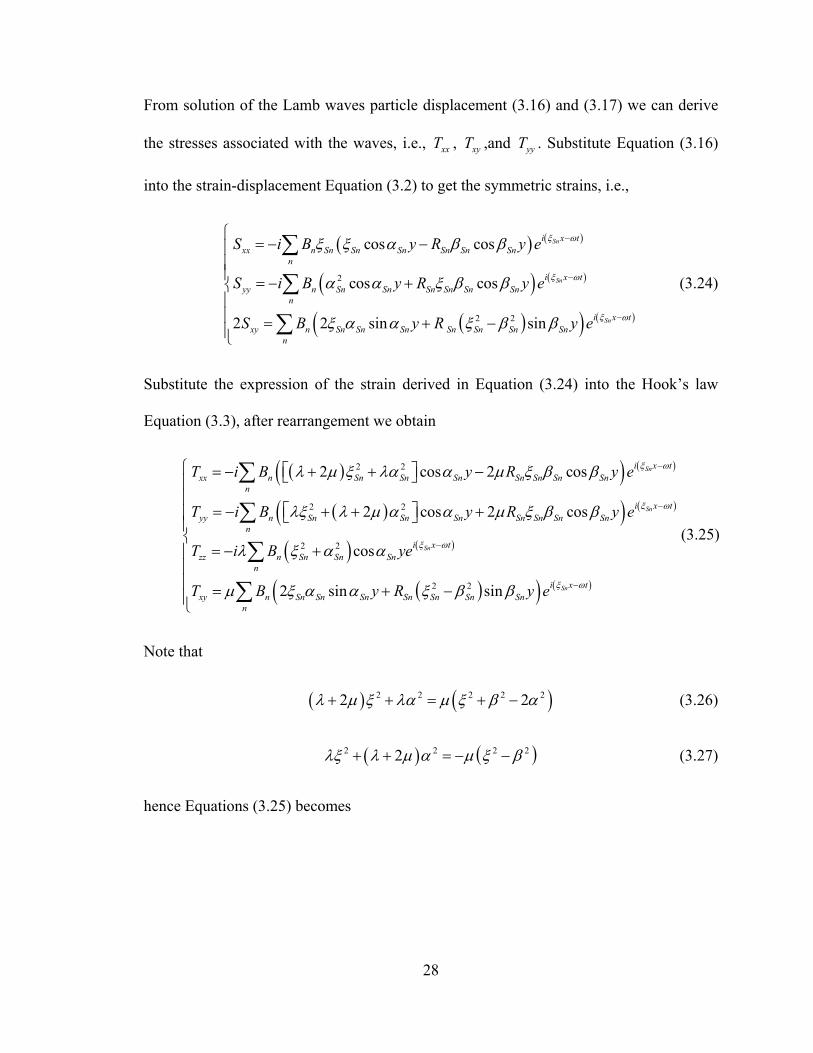
28
From solution of the Lamb waves particle displacement (3.16) and (3.17) we can derive
the stresses associated with the waves, i.e., xxT , xyT ,and yyT . Substitute Equation (3.16)
into the strain-displacement Equation (3.2) to get the symmetric strains, i.e.,
( ) ( )
( ) ( )
( )( ) ( )
2
2 2
cos cos
cos cos
2 2 sin sin
Sn
Sn
Sn
i x txx n Sn Sn Sn Sn Sn Sn
n
i x tyy n Sn Sn Sn Sn Sn Sn
n
i x txy n Sn Sn Sn Sn Sn Sn Sn
n
S i B y R y e
S i B y R y e
S B y R y e
ξ ω
ξ ω
ξ ω
ξ ξ α β β
α α ξ β β
ξ α α ξ β β
−
−
−
⎧= − −⎪
⎪⎪ = − +⎨⎪⎪ = + −⎪⎩
∑
∑
∑
(3.24)
Substitute the expression of the strain derived in Equation (3.24) into the Hook’s law
Equation (3.3), after rearrangement we obtain
( )( ) ( )
( )( ) ( )
( ) ( )
( )
2 2
2 2
2 2
2 2
2 cos 2 cos
2 cos 2 cos
cos
2 sin sin
Sn
Sn
Sn
i x txx n Sn Sn Sn Sn Sn Sn Sn
n
i x tyy n Sn Sn Sn Sn Sn Sn Sn
n
i x tzz n Sn Sn Sn
n
xy n Sn Sn Sn Sn Sn Sn
T i B y R y e
T i B y R y e
T i B ye
T B y R
ξ ω
ξ ω
ξ ω
λ μ ξ λα α μ ξ β β
λξ λ μ α α μ ξ β β
λ ξ α α
μ ξ α α ξ β β
−
−
−
⎡ ⎤= − + + −⎣ ⎦
⎡ ⎤= − + + +⎣ ⎦
= − +
= + −
∑
∑
∑
( ) ( )Sni x tSn
ny e ξ ω−
⎧⎪⎪⎪⎪⎨⎪⎪⎪⎪⎩
∑
(3.25)
Note that
( ) ( )2 2 2 2 22 2λ μ ξ λα μ ξ β α+ + = + − (3.26)
( ) ( )2 2 2 22λξ λ μ α μ ξ β+ + = − − (3.27)
hence Equations (3.25) becomes

29
( ) ( )
( ) ( )
( ) ( )
( )( )
2 2 2
2 2
2 2
2 2
2 cos 2 cos
cos 2 cos
cos
2 sin sin
Sn
Sn
Sn
i x txx n Sn Sn Sn Sn Sn Sn Sn Sn
n
i x tyy n Sn Sn Sn Sn Sn Sn Sn
n
i x tzz n Sn Sn Sn
n
ixy n Sn Sn Sn Sn Sn Sn Sn
T i B y R y e
T i B y R y e
T i B ye
T B y R y e
ξ ω
ξ ω
ξ ω
μ ξ β α α ξ β β
μ ξ β α ξ β β
λ ξ α α
μ ξ α α ξ β β
−
−
−
⎡ ⎤= − + − −⎣ ⎦
⎡ ⎤= − −⎣ ⎦
= − +
= + −
∑
∑
∑( )Sn x t
n
ξ ω−
⎧⎪⎪⎪⎪⎨⎪⎪⎪⎪⎩
∑
(3.28)
Likewise, to obtain the antisymmetric stresses substitute Equation (3.17) into the strain-
displacement Equation (3.2) to get the antisymmetric strains, i.e.,
( ) ( )
( ) ( )
( )( ) ( )
2
2
2 2
sin sin
sin sin
2 2 cos cos
An
An
An
i x txx n An An An An An An
n
i x tyy n An An An An An An
n
i x txy n An An An An An An An
n
S i A y R y e
S i A y R y e
S A y R y e
ξ ω
ξ ω
ξ ω
ξ α ξ β β
α α ξ β β
ξ α α ξ β β
−
−
−
⎧= − −⎪
⎪⎪ = − +⎨⎪⎪ = − + −⎪⎩
∑
∑
∑
(3.29)
Substitute the expression of the strain derived in Equation (3.29) into the Hook’s law
Equation (3.3), after rearrangement we obtain
( )( ) ( )
( )( ) ( )
( )( )( )
2 2
2 2
2 2
2 2
2 sin 2 sin
2 sin 2 sin
sin
2 cos cos
An
An
An
i x txx n An An An An An An An
n
i x tyy n An An An An An An An
n
zz n An An Ann
i xxy n An An An An An An An
T i A y R y e
T A y R y e
T i A y
T A y R y e
ξ ω
ξ ω
ξ
λ μ ξ λα α μ ξ β β
λξ λ μ α α μ ξ β β
λ ξ α α
μ ξ α α ξ β β
−
−
⎡ ⎤= − + + −⎣ ⎦
⎡ ⎤= − + + +⎣ ⎦
= − +
= − + −
∑
∑
∑( )t
n
ω−
⎧⎪⎪⎪⎪⎨⎪⎪⎪⎪⎩
∑
(3.30)
Substitute Equations (3.26) and (3.27) into (3.30) to get

30
( ) ( )
( ) ( )
( )( )( ) ( )
2 2 2
2 2
2 2
2 2
2 sin 2 sin
sin 2 sin
sin
2 cos cos
An
An
An
i x txx n An An An An An An An An
n
i x tyy n An An An An An An An
n
zz n An An Ann
i x txy n An An An An An An An
n
T i A y R y e
T A y R y e
T i A y
T A y R y e
ξ ω
ξ ω
ξ ω
μ ξ β α α ξ β β
μ ξ β α ξ β β
λ ξ α α
μ ξ α α ξ β β
−
−
−
⎡ ⎤= − + − −⎣ ⎦
⎡ ⎤= − −⎣ ⎦
= − +
= − + −
∑
∑
∑
∑
⎧⎪⎪⎪⎪⎨⎪⎪⎪⎪⎩
(3.31)
3.1.7 Approximate simplified solution
In this section, we present the simplified solution for axial and flexural waves, i.e. low
frequency range of S0 and A0 modes. For the case of the flexural wave, we will derive
the solution with and without the Euler-Bernoulli assumption.
3.1.7.1 Straight-crested wave plates: axial and shear waves
Consider a differential element of plate thickness t=2d subjected to normal and shear
forces as shown in Figure 3.5.
Figure 3.5 An element of plate subjected to forces (after Giurgiutiu, 2008)
The equations of motion are given by the equilibrium of forces of the plate element, i.e.,
2
2
2
2
x xzx x xz xz
z xzz z xz xz
N N uN dz N dx dz N dx N dz dx tdxdzx z t
N N wN dx N dz dx N dz N dx dz tdxdzz x t
ρ
ρ
⎧ ∂ ∂ ∂⎛ ⎞ ⎛ ⎞− + + − + + =⎜ ⎟ ⎜ ⎟⎪ ∂ ∂ ∂⎪ ⎝ ⎠ ⎝ ⎠⎨
∂ ∂ ∂⎛ ⎞ ⎛ ⎞⎪− + + − + + =⎜ ⎟ ⎜ ⎟⎪ ∂ ∂ ∂⎝ ⎠ ⎝ ⎠⎩
(3.32)
xx
NN dxx
∂+
∂xN
xzN
xzN
xzxz
NN dxx
∂+
∂
xzxz
NN dzz
∂+
∂
zN
zz
NN dz
z∂
+∂
dxdz x
z
y
dxdz

31
where u is the displacement in the x direction and w is the displacement in the z direction.
Cancelling the terms, the equation of motion reduces to
2
2
2
2
x xz
z xz
N N utx z t
N N wtz x t
ρ
ρ
⎧∂ ∂ ∂+ =⎪⎪ ∂ ∂ ∂
⎨∂ ∂ ∂⎪ + =⎪ ∂ ∂ ∂⎩
(3.33)
We assume that displacements u and w are uniform across the thickness. The force
resultants per unit width are given by
( , )
( , )
( , )
d
x xxdd
xz xzdd
z zzd
N T x z dy
N T x z dy
N T x z dy
−
−
−
⎧ =⎪⎪
=⎨⎪⎪ =⎩
∫∫∫
(3.34)
Recall the definition of the stresses, Equation (2.14), and consider normal stresses and the
shear stress xzT , i.e.,
( )( )
( )
2
2
2
2
xx xx yy zz
yy xx yy zz
zz xx yy zz
xz xz
T S S S
T S S S
T S S S
T S
λ μ λ λ
λ λ μ λ
λ λ λ μ
μ
⎧ = + + +⎪
= + + +⎪⎨
= + + +⎪⎪ =⎩
(3.35)
For free top and bottom surfaces, the stress in the y direction is assumed to be zero
( 0yyT = ) hence, solving the second equation in Equation (3.35), we obtain after
rearrangement

32
( )
242 2
22 4
2 22
xx xx zz
yy xx zz
zz xx zz
xz xz
T S S
S S S
T S S
T S
λ μ λμμλ μ λ μ
λλ μλμ λ μμ
λ μ λ μμ
+⎧ = +⎪ + +⎪⎪ = − +⎪ +⎨⎪ +
= +⎪+ +⎪
⎪ =⎩
(3.36)
Recalling the Lame relations defined as
( )( )
( )
1 1 2
2 1
E
EG
νλν ν
μν
⎧ =⎪ + −⎪⎨⎪ = =⎪ +⎩
(3.37)
the stress-strain relation, Equation (3.36), can be written as
( )
( )
( )
( )
2
2
1
1
1
22 1
xx xx zz
yy xx zz
zz xx zz
xz xz
ET S S
S S S
ET S S
ET S
ννν
ν
νν
ν
⎧ = +⎪ −⎪⎪ = − +⎪ −⎨⎪ = +⎪ −⎪⎪ =
+⎩
(3.38)
Substitute the stress-strain relation defined in Equation (3.38) and the strain-displacement
relation, Equation (3.3), into the force resultants, Equation (3.34), to get
( ) ( )
2 2
2 2
1 1
2 1 2 1
1 1
d
x d
d
xz d
d
z d
E u w Et u wN dyx z x z
E u w Et u wN dyz x z x
E u w Et u wN dyx z x z
ν νν ν
ν ν
ν νν ν
−
−
−
⎧ ∂ ∂ ∂ ∂⎛ ⎞ ⎛ ⎞= + = +⎜ ⎟ ⎜ ⎟⎪ − ∂ ∂ − ∂ ∂⎝ ⎠ ⎝ ⎠⎪∂ ∂ ∂ ∂⎪ ⎛ ⎞ ⎛ ⎞= + = +⎜ ⎟ ⎜ ⎟⎨ + ∂ ∂ + ∂ ∂⎝ ⎠ ⎝ ⎠⎪
⎪ ∂ ∂ ∂ ∂⎛ ⎞ ⎛ ⎞= + = +⎜ ⎟ ⎜ ⎟⎪ − ∂ ∂ − ∂ ∂⎝ ⎠ ⎝ ⎠⎩
∫
∫
∫
(3.39)

33
Substitute Equation (3.39) into (3.33) to get the equilibrium equation in terms of the
particle displacements only, i.e.,
( )
( )
2 2 2 2 2
2 2 2 2
2 2 2 2 2
2 2 2 2
1 11 2 1
1 11 2 1
u w u w ux x z z x z E t
u w u w wx z z x z x E t
ρνν ν
ρνν ν
⎧ ⎛ ⎞ ⎛ ⎞∂ ∂ ∂ ∂ ∂+ + + =⎜ ⎟ ⎜ ⎟⎪ − ∂ ∂ ∂ + ∂ ∂ ∂ ∂⎪ ⎝ ⎠ ⎝ ⎠
⎨⎛ ⎞ ⎛ ⎞∂ ∂ ∂ ∂ ∂⎪ + + + =⎜ ⎟ ⎜ ⎟⎪ − ∂ ∂ ∂ + ∂ ∂ ∂ ∂⎝ ⎠ ⎝ ⎠⎩
(3.40)
If we consider the problem to be z-invariant, Equation (3.40) simplifies to
2 2
2 2 2
2 2
2 2 2
1
1L
S
u ux c t
w wx c t
⎧∂ ∂=⎪∂ ∂⎪
⎨∂ ∂⎪ =⎪ ∂ ∂⎩
(3.41)
where ( )2 21Lc E ρ ν⎡ ⎤= −⎣ ⎦ is the axial (or longitudinal) wave velocity and
( )[ ]2 2 1Sc E Gρ ν ρ= + = is the shear wave velocity. The first equation in (3.41) is
characterized by the axial displacement u only and it represents the equation of motion
for axial waves in plates; the second equation in (3.41) is characterized by the transverse
displacement w only and it represents the equation of motion for shear waves in plates.
3.1.7.2 Flexural waves
To derive the flexural waves, consider a differential element of plate thickness 2d. Figure
3.6 shows the moments and forces acting on the element.

34
Figure 3.6 An element of plate subjected to forces and moments (after Graff, 1991)
where v is the displacement in the y direction. Cancelling the terms, the equations of
motion reduce to
2
2
0
0
x z
x zxx
xzzz
Q Q vtx z t
M M Qx x
MM Qz z
ρ⎧∂ ∂ ∂
+ =⎪ ∂ ∂ ∂⎪⎪∂ ∂
+ − =⎨∂ ∂⎪
⎪ ∂∂− − =⎪ ∂ ∂⎩
(3.42)
Differentiate the second and third equations in Equation (3.42) and substitute the result in
the first to obtain the equilibrium relation in terms of moments, i.e.,
2 2 22 2
2 2 2x zx xzzM M MM vt
x z x zx z tρ∂ ∂ ∂∂ ∂
+ + − =∂ ∂ ∂ ∂∂ ∂ ∂
(3.43)
To solve the equation of motion, we must establish the relationship between moments
and deflections. We introduce the kinematics of the deformation, in particular we assume
that, when the element is subjected to pure bending, it deforms such as plane sections
remain plane and perpendicular to the mid plane (Euler-Bernoulli assumption). The
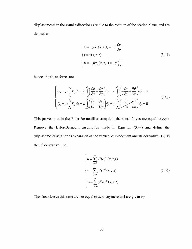
35
displacements in the x and z directions are due to the rotation of the section plane, and are
defined as
( , , )
( , , )
( , , )
x
z
vu y x z t yx
v v x z tvw y x z t yz
ψ
ψ
∂⎧ = − = −⎪ ∂⎪=⎨
⎪ ∂⎪ = − = −∂⎩
(3.44)
hence, the shear forces are
d d
x xyd d
u v v vQ T dz dyy x x x
μ μ μ− −
∂ ∂ ∂ ∂⎛ ⎞ ⎛ ⎞= = + = − +⎜ ⎟⎜ ⎟∂ ∂ ∂ ∂⎝ ⎠⎝ ⎠∫ ∫ 0
d
dd d
z yzd d
dy
v w v vQ T dz dyz y z z
μ μ μ
−
− −
=
∂ ∂ ∂ ∂⎛ ⎞ ⎛ ⎞= = + = − +⎜ ⎟⎜ ⎟∂ ∂ ∂ ∂⎝ ⎠⎝ ⎠
∫
∫ ∫ 0d
d
dy−
⎧⎪⎪⎨⎪ =⎪⎩
∫ (3.45)
This proves that in the Euler-Bernoulli assumption, the shear forces are equal to zero.
Remove the Euler-Bernoulli assumption made in Equation (3.44) and define the
displacements as a series expansion of the vertical displacement and its derivative ( ( )n is
the nth derivative), i.e.,
( )
0
( )
0
( )
0
( , , )
( , , )
( , , )
n nx
n
n n
n
n nz
n
u y x z t
v y v x z t
w y x z t
ψ
ψ
∞
=
∞
=
∞
=
⎧=⎪
⎪⎪⎪ =⎨⎪⎪⎪ =⎪⎩
∑
∑
∑
(3.46)
The shear forces this time are not equal to zero anymore and are given by

36
( )1 ( )
0 0
( )1 ( )
0 0
d d d nn n n
x xy xn nd d d
d d d nn n n
z yz zn nd d d
u v vQ T dz dz ny y dyy x x
w v vQ T dz dz ny y dyy z x
μ μ ψ
μ μ ψ
∞ ∞−
= =− − −
∞ ∞−
= =− − −
⎧ ⎛ ⎞∂ ∂ ∂⎛ ⎞= = + = +⎪ ⎜ ⎟⎜ ⎟∂ ∂ ∂⎝ ⎠ ⎝ ⎠⎪⎨
⎛ ⎞∂ ∂ ∂⎛ ⎞⎪ = = + = +⎜ ⎟⎜ ⎟⎪ ∂ ∂ ∂⎝ ⎠ ⎝ ⎠⎩
∑ ∑∫ ∫ ∫
∑ ∑∫ ∫ ∫ (3.47)
The form of the shear stress depends on the truncation of the power series. This is the
formulation for the Timoshenko beam theory that we will not pursue further. Under the
Euler-Bernoulli assumption, the moments can be defined as
d
x xxd
d
z zzd
d
xz zx xzd
M T ydy
M T ydy
M M T ydy
−
−
−
⎧=⎪
⎪⎪⎪ =⎨⎪⎪⎪ = − = −⎪⎩
∫
∫
∫
(3.48)
Substitute the strain-displacement relation (3.3) and the displacement definition, Equation
(3.44), into the stress equation in Equation (3.38) to obtain
( )
2 2
2 2 2
2 2
2 2
2 2
2 2 2
2
1
1
12
1
xx
yy
zz
xz
E v vT yx z
v vS yx z
E v vT yx z
E vT yx z
νν
νν
νν
ν
⎧ ⎛ ⎞∂ ∂= − +⎜ ⎟⎪ − ∂ ∂⎝ ⎠⎪
⎪ ⎛ ⎞∂ ∂= +⎪ ⎜ ⎟⎪ − ∂ ∂⎝ ⎠
⎨⎛ ⎞∂ ∂⎪ = − +⎜ ⎟⎪ − ∂ ∂⎝ ⎠
⎪∂⎪ = −⎪ + ∂ ∂⎩
(3.49)
With the use of Equation (3.49), Equation (3.48) yields

37
( )( )
2 2 2 22
2 2 2 2 2
2 2 2 22
2 2 2 2 2
2 22
1
1
2 11
d
xd
d
zd
d
xz zxd
E v v v vM y dy Dx z x z
E v v v vM y dy Dx z x z
E v vM M y dy Dx z x z
ν νν
ν νν
νν
−
−
−
⎧ ⎛ ⎞ ⎛ ⎞∂ ∂ ∂ ∂= − + = − +⎪ ⎜ ⎟ ⎜ ⎟− ∂ ∂ ∂ ∂⎝ ⎠ ⎝ ⎠⎪
⎪ ⎛ ⎞ ⎛ ⎞∂ ∂ ∂ ∂⎪ = − + = − +⎨ ⎜ ⎟ ⎜ ⎟− ∂ ∂ ∂ ∂⎝ ⎠ ⎝ ⎠⎪⎪ ∂ ∂⎪ = − = = −⎪ + ∂ ∂ ∂ ∂⎩
∫
∫
∫
(3.50)
where D is the flexural plate stiffness defined as ( )3 22 3 1D Ed ν⎡ ⎤= −⎣ ⎦ . With the use of
Equation (3.50), the equation of motion (3.43) becomes
4 4 4 2
4 2 2 4 4 212F
v v v vx x z z c t
∂ ∂ ∂ ∂+ + = −
∂ ∂ ∂ ∂ ∂ (3.51)
where cF is the flexural wave speed defined as ( )4Fc D tρ= . For straight crested flexural
wave, the problem is z-invariant, hence Equation (3.51) becomes
4 2
4 4 21
F
v vx c t
∂ ∂= −
∂ ∂ (3.52)
3.2 CIRCULAR-CRESTED GUIDED WAVES IN CYLINDRICAL COORDINATES
In this section, we perform the derivation of circular-crested guided waves in cylindrical
coordinate system. A detailed derivation of the solution of the acoustic field equations is
provided. For the case of Lamb waves solution, the derivation of the solution follows that
shown in Goodman (1951) and Giurgiutiu (2008) with the exception of assuming that the
solution follows sine and cosine functions instead of hyperbolic functions. This
difference allows us to show in a simpler way the similarities between the straight crested
solution and the circular crested one.

38
Consider a cylindrical coordinate system such as that the r coordinate is along the
wave propagation and the z coordinate is parallel to the thickness of the plate. Figure 3.7
shows the coordinate system.
Figure 3.7 Cylindrical wave notations
3.2.1 Equation of motion
Recall the equation of motion expressed in Equation (2.1), i.e.,
2
2tδρδ
∇ ⋅ = −uT F (3.53)
Assume θ-invariance such as 0θ∂
=∂
, use relation in Equation (2.9) and express the
equation of motion in extended form, i.e.,
2
2
2
2
2
2
1
1
1
rr rz rr
r z r
rz zz zz
TrT T u Fr r z r t
rT T T u Fr r z r t
rT T u Fr r z t
θθ
θ θ θ θθ
ρ
ρ
ρ
⎧ ∂ ∂ ∂+ − = −⎪ ∂ ∂ ∂⎪
⎪ ∂ ∂ ∂+ + = −⎨
∂ ∂ ∂⎪⎪ ∂ ∂ ∂
+ = −⎪∂ ∂ ∂⎩
(3.54)
or, by performing the derivate with respect to r,
r
z
Wave front
z d= +
z d= −
θ

39
2
2
2
2
2
2
2
rrrr rz rr
r z r
rz zz rz zz
T TT T u Fr z r t
T T T u Fr z r t
T T T u Fr z r t
θθ
θ θ θ θθ
ρ
ρ
ρ
⎧ −∂ ∂ ∂+ + = −⎪ ∂ ∂ ∂⎪
⎪∂ ∂ ∂+ + = −⎨
∂ ∂ ∂⎪⎪∂ ∂ ∂
+ + = −⎪∂ ∂ ∂⎩
(3.55)
System (3.55) has three equations: the first and third equations are coupled through the
term rzT , while the third is uncoupled from the others. As in rectangular coordinates, the
coupled equations are the equations of motion for circular crested Lamb waves. These
waves propagate along the r coordinate and they have particle displacement in both the r
and z direction (denoted by ru and zu respectively). The second equation in system
(3.55) represents the equation of motion for circular crested SH waves. The SH waves
propagate along the r direction with particle displacement along the θ direction (denoted
by uθ ). The Lamb waves equation of motion and the SH wave equation of motion can be
solved separately.
3.2.2 Strain-displacement equation
Consider the strain-velocity relation (2.10), with the use of Equation (2.12) and the θ-
invariant condition, this can be expanded as
rrr
r
zzz
uSr
uSruSz
θθ
∂⎧ =⎪ ∂⎪⎪ =⎨⎪
∂⎪ =⎪ ∂⎩
2
2
12
z
r zrz
r
uSz
u uSz ruS ur r
θθ
θθ θ
∂⎧ =⎪ ∂⎪∂ ∂⎪ = +⎨ ∂ ∂⎪∂⎪
= −⎪ ∂⎩
(3.56)
In Equation (3.55) we have seen that the terms in rr , rz , and zz are not coupled with
the terms in rθ , and zθ , hence, the third and fifth equation in (3.56) are decoupled from

40
the other three and they represent the strain-displacement relations for SH waves.
Likewise, the first, second and fourth equations represent the Lamb wave strain-
displacement relations.
Note that in cylindrical coordinates the strain along the invariant coordinate (θ ) is not
equal to zero.
3.2.3 Hooke’s law
Assume θ-invariant condition such as 0uθ
θ∂
=∂
. Substitute in the equation of Hook’s law
(2.14) the stiffness matrix (2.16) to obtain the stress-strain relation in cylindrical
coordinates, i.e.,
( )( )( )
11 12 13
12 22 23
13 12 33
44
55
66
2
2
22 22 22 2
rr rr zz rr zz
rr zz rr zz
zz rr zz rr zz
z z z
rz rz rz
r r r
T c S c S c S S S S
T c S c S c S S S S
T c S c S c S S S ST c S ST c S ST c S S
θθ θθ
θθ θθ θθ
θθ θθ
θ θ θ
θ θ θ
λ μ λ λ
λ λ μ λ
λ λ μ λμ
μμ
⎧ = + + = + + +⎪
= + + = + + +⎪⎪ = + + = + + +⎪⎨
= =⎪⎪ = =⎪
= =⎪⎩
(3.57)
3.2.4 Acoustic field equations
The acoustic filed equations are derived by substituting Hook’s law Equation (3.57) into
the Equation of motion (3.55), after rearrangement of the terms, we obtain
( )
( )
2
2
2
2
2
2
2 2 2
2 2 4
2 2 2
rrrr zz rz rr
r z r
rz rr zz rz zz
S S SS S S u Fr r r z r t
S S S u Fr z r t
SS S S S u Fr z z z r t
θθ θθ
θ θ θ θθ
θθ
λ μ λ λ μ μ ρ
μ μ μ ρ
μ λ λ μ λ μ ρ
⎧ ∂ −∂ ∂ ∂ ∂+ + + + + = −⎪ ∂ ∂ ∂ ∂ ∂⎪
⎪ ∂ ∂ ∂+ + = −⎨
∂ ∂ ∂⎪⎪ ∂∂ ∂ ∂ ∂
+ + + + + = −⎪∂ ∂ ∂ ∂ ∂⎩
(3.58)

41
Substitute the strain-displacement Equation (3.56) into (3.58) and rearrange the terms to
obtain the acoustic field equations in cylindrical coordinates
( ) ( ) ( ) ( )
( ) ( ) ( )
2 2 2 2
2 2 2 2
2 2 2
2 2 2 2
2 2 2 2
2 2 2
12 2 2
1
1 12
r r r z r rr
r r z z z zz
u u u u u u Fr r r r r z z t
u u u u u Fr z r r r t
u u u u u u Fr z r z r z r r t
θ θ θ θ θθ
λ μ λ μ λ μ λ μ μ ρ
μ μ μ μ ρ
λ μ λ μ μ λ μ μ ρ
⎧ ∂ ∂ ∂ ∂ ∂+ − + + + + + + = −⎪ ∂ ∂ ∂ ∂ ∂ ∂⎪
⎪ ∂ ∂ ∂ ∂+ + − = −⎨
∂ ∂ ∂ ∂⎪⎪ ∂ ∂ ∂ ∂ ∂ ∂
+ + + + + + + = −⎪∂ ∂ ∂ ∂ ∂ ∂ ∂⎩
(3.59)
The uncoupling between the acoustic wave equations is even more evident in Equation
(3.59). The first and third equation depend on both r and z coordinates and they represent
the Lamb wave equations. The second equation in (3.59) depends only on θ coordinate
and it represents SH waves equation. The Lamb waves equations of motion and the SH
waves equation of motion can be solved separately.
To derive the particle displacement we consider a plate not subject to body forces,
hence 0=F . Moreover, we assume that the top and bottom surfaces of the plate are free
surfaces, hence the boundary conditions are
0
0
0
zz z d
rz z d
z z d
T
T
Tθ
=±
=±
=±
⎧ =⎪⎪ =⎨⎪ =⎪⎩
(3.60)
3.2.5 Shear horizontal waves solutions
Solution to the SH waves equation is found from the second equation in (3.59), i.e.,
2 2 2
2 2 2 2 2
1 1
s
u u u u ur z r r r c t
θ θ θ θ θ∂ ∂ ∂ ∂+ + − =
∂ ∂ ∂ ∂ (3.61)
The displacement is assumed to be harmonic both in time and in the z coordinate, i.e.

42
( )( , , ) ( ) i z tu r z t g r e β ωθ ξ −= (3.62)
where 2 2 2 2scη ω ξ= − . Substitute solution (3.62) into Equation (3.61), divide by ( )i z te η ω− ,
and rearrange the terms to obtain
2
22 2
( ) 1 ( ) 1 ( ) 0g r g r g rr r r rξ ξ ξ ξ∂ ∂ ⎛ ⎞+ + − =⎜ ⎟
∂ ∂ ⎝ ⎠ (3.63)
Perform the following coordinate substitution
rζ ξ= (3.64)
Equation (3.63) becomes
2
22 2
( ) 1 ( ) 11 ( ) 0g g gζ ζξ ζζ ζ ζ ζ
⎡ ⎤∂ ∂ ⎛ ⎞+ + − =⎢ ⎥⎜ ⎟∂ ∂ ⎝ ⎠⎣ ⎦ (3.65)
Solution of Equation (3.65) is the Bessel function of order 1p = , i.e.,
( )1( )g r AJ rξ ξ= (3.66)
Hence, solution to Equation (3.61) takes the form
( )1( , , ) ( ) sin cos i tu r z t J r A z B z e ωθ ξ β β −= + (3.67)
Equation (3.67) must satisfy the stress-free top and bottom surfaces boundary conditions,
i.e.,
( ) 0zd
udzθ
θτ±
∂± = =
∂ (3.68)
Substitute solution (3.67) into the boundary conditions (3.68) to obtain

43
sin cos 0
sin cos 0A d B d
A d B dη η
η η+ =⎧
⎨− + =⎩ (3.69)
This system has nontrivial solution if the determinant equals zero, hence
sin cos 0d dη η = (3.70)
Solution to Equation (3.70) is given by
( ) ( )
22
2 1 2
S
A
nd
n d
πη
η π
⎧ =⎪⎨⎪ = +⎩
1, 2,n = L (3.71)
where, as usual, subscript S is for symmetric modes and subscript A is for antisymmetric
modes. Constant nA and nB can be found through the normalization as discussed in
Appendix E. Particle displacement (3.67) can now be written in extended form as
( )1 1( , , ) ( )sin ( )cosS A A A i tn n n n n n
nu r z t A J r z B J r z e ω
θ ξ η ξ η −= +∑ (3.72)
Particle displacement (3.72) behaves as 1( )J rξ in the radial direction. As r increases the
amplitude of the displacement decreases as
( )5 2 rπ (3.73)
The amplitude of the unit energy per circumferential length released by the source
decreases as the circular crested wave travels outward since the length of the wave front
increases as 2 rπ . However, if we consider the total circumferential energy this is given
by 2ruθπ , with the use of Equation (3.73), we see that the total energy is constant. Refer
to Appendix C for more details.

44
From the solution of SH waves particle displacement (3.72), we can derive the
stresses associated with the SH waves, i.e., rT θ and zTθ . Substitute Equation (3.72) into
the strain-displacement Equation (3.56) to get, after rearrangement,
( )1 1
0 1
0 1
2 cos ( ) cos ( )
2sin ( ) ( )2
2cos ( ) ( )
A A S A A A i tz n n n n n n n n
n
A S S Sn n n n n
i tr
n A A A An n n n n
S A zJ r B zJ r e
A z J r J rrS e
B z J r J rr
ωθ
ωθ
η η ξ η η ξ
η ξ ξ ξ
η ξ ξ ξ
−
−
⎧ = −⎪⎪ ⎛ ⎞⎡ ⎤⎪ −⎜ ⎟⎨ ⎢ ⎥⎣ ⎦⎜ ⎟⎪ =
⎜ ⎟⎪ ⎡ ⎤+ −⎜ ⎟⎪ ⎢ ⎥⎣ ⎦⎝ ⎠⎩
∑
∑ (3.74)
Substitute the expression of the strain in the stress-strain relation (3.57) to get
( )1 1
0 1
0 1
cos ( ) cos ( )
2sin ( ) ( )
2cos ( ) ( )
A A S A A A i tz n n n n n n n n
n
A S S Sn n n n n
i tr
n A A A An n n n n
T A zJ r B zJ r e
A z J r J rrT e
B z J r J rr
ωθ
ωθ
μ η η ξ η η ξ
η ξ ξ ξμ
η ξ ξ ξ
−
−
⎧ = −⎪⎪ ⎛ ⎞⎡ ⎤⎪ −⎜ ⎟⎨ ⎢ ⎥⎣ ⎦⎜ ⎟⎪ =
⎜ ⎟⎪ ⎡ ⎤+ −⎜ ⎟⎪ ⎢ ⎥⎣ ⎦⎝ ⎠⎩
∑
∑ (3.75)
Note that the behavior in the thickness direction of the particle displacement and that of
the stresses are the same in both rectangular and cylindrical coordinates. This was to be
expected since the derivation in rectangular coordinates is a particular case of that in
cylindrical coordinates: as the radial distance goes to infinity, the Bessel functions
become periodic and with constant amplitude and the term 1 0r → .
3.2.6 Lamb waves solutions
Solution for the circular crested Lamb waves are found from the first and third equations
in (3.59) assuming volume forces equal to zero, i.e.,

45
( ) ( ) ( ) ( )
( ) ( ) ( )
2 2 2 2
2 2 2 2
2 2 2 2
2 2 2
12 2 2
1 12
r r r z r r
r r z z z z
u u u u u ur r r r r z z t
u u u u u ur z r z r z r r t
λ μ λ μ λ μ λ μ μ ρ
λ μ λ μ μ λ μ μ ρ
⎧ ∂ ∂ ∂ ∂ ∂+ − + + + + + + =⎪⎪ ∂ ∂ ∂ ∂ ∂ ∂
⎨∂ ∂ ∂ ∂ ∂ ∂⎪ + + + + + + + =⎪ ∂ ∂ ∂ ∂ ∂ ∂ ∂⎩
(3.76)
The wave equations can be expressed in terms of the dilatation Δ and the displacement
particles in radial and vertical directions. Recall that the dilatation of a material is defined
by
rr zzS S SθθΔ = + + (3.77)
With the use of (3.77) and the equation of motion defined in terms of strain, see Equation
(3.58), we obtain
( )
( )
2
2
2
2
2 2
2 2
rrrr zz rz r
rr zz rz rz z
S S SS S S ur r r r z r t
SS S S S uz z z z r r t
θθ θθ
θθ
λ μ μ μ μ μ μ ρ
λ μ μ μ μ μ μ ρ
⎧ ∂ −∂ ∂ ∂ ∂∂Δ+ + − − + + =⎪⎪ ∂ ∂ ∂ ∂ ∂ ∂
⎨∂∂ ∂ ∂ ∂∂Δ⎪ + − + − + + =⎪ ∂ ∂ ∂ ∂ ∂ ∂⎩
(3.78)
Equation (3.78) can be rearranged in this form
( )
( )
2
2
2
2
2 2 2 2 2
2 2 2 2 2
rrzz rz r
rr rz rz z
S S SS S ur r r z r t
S S S S uz z z r r t
θθ θθ
θθ
λ μ μ μ μ μ ρ
λ μ μ μ μ μ ρ
⎧ ∂ −∂ ∂ ∂∂Δ+ − − + + =⎪⎪ ∂ ∂ ∂ ∂ ∂
⎨∂ ∂ ∂ ∂∂Δ⎪ + − − + + =⎪ ∂ ∂ ∂ ∂ ∂⎩
(3.79)
The terms in strain can be proved to be equal to the curl of the rotation vector ω , i.e.,
( )
( )2 2
2
1 1 ˆ2 2
1 1 1 1 ˆ2 2
rrzz rz r z
rr rz rz r r z z
S S SS S u ur r z r z z r
S S S S u u u uz z r r r z r z r r r
θθ θθ
θθ
⎧ ∂ −∂ ∂ ∂ ∂∂ ⎛ ⎞− − + + = − = − ∇× ⋅⎜ ⎟⎪ ∂ ∂ ∂ ∂ ∂ ∂⎝ ⎠⎪⎨
⎛ ⎞∂ ∂ ∂ ∂ ∂ ∂ ∂⎪− − + + = − − + + = − ∇× ⋅⎜ ⎟⎪ ∂ ∂ ∂ ∂ ∂ ∂ ∂ ∂⎝ ⎠⎩
ω r
ω z(3.80)
where the curl of the rotation vector is defined as

46
1 1ˆˆ ˆ
1ˆˆ ˆ
z r z r
r z
u ruu u u ur z z r r r
u ruu uz z r r r
θ θ
θ θ
θ θ∂ ∂∂ ∂ ∂ ∂⎛ ⎞ ⎛ ⎞⎛ ⎞= ∇× = − + − + −⎜ ⎟ ⎜ ⎟ ⎜ ⎟∂ ∂ ∂ ∂ ∂ ∂⎝ ⎠ ⎝ ⎠ ⎝ ⎠
∂ ∂∂ ∂⎛ ⎞= − + − +⎜ ⎟∂ ∂ ∂ ∂⎝ ⎠
ω u r θ z
r θ z (3.81)
Hence, Equation (3.78) becomes
( ) ( )
( ) ( )
2
2
2
2
ˆ2
ˆ2
r
z
ur t
uz t
λ μ μ ρ
λ μ μ ρ
⎧ ∂∂Δ+ − ∇× ⋅ =⎪⎪ ∂ ∂
⎨∂∂Δ⎪ + − ∇× ⋅ =⎪ ∂ ∂⎩
ω r
ω z (3.82)
or more generically
( ) ( )2
22t
λ μ μ ρ ∂+ ∇Δ − ∇× =
∂uω (3.83)
If the vector operation divergence is performed on the above, we obtain
( ) ( )2
222
tλ μ μ ρ ∂ ∇ ⋅
+ ∇ Δ − ∇ ⋅ ∇× =∂
uω (3.84)
Note that Equation (3.84) becomes
( )2
222
tλ μ ρ ∂ Δ
+ ∇ Δ =∂
(3.85)
since
( )1 z r r zr
u u u urur r z r r z
∂ ∂ ∂∂∇ ⋅ = + = + + = Δ
∂ ∂ ∂ ∂u (3.86)
and ( ) 0∇ ⋅ ∇× = where
2
22
1 rr r r z
∂ ∂ ∂⎛ ⎞∇ = +⎜ ⎟∂ ∂ ∂⎝ ⎠ (3.87)

47
Hence, the dilatation terms must satisfy the wave Equation (3.85) (Helmholtz equation).
We assume the dilatation to take two forms
( )0
cossin
i t zA J r e
zω αμ ξ
αλ μ− ⎧
Δ = ⎨+ ⎩ (3.88)
where 0 ( )J rξ is the Bessel function of order zero. The first form of the dilatation
corresponds to extensional wave propagation; the second form corresponds to the flexural
wave propagation. Substitute Equation (3.88) into the Helmholtz Equation (3.85) to get
( )( ) ( )
202
00 2 2 2
coscos cossinsin sin
i ti t i t
p
zJ rr z zz J rA er e J r ez zr r z c t
ωω ω
αξα αα ξμ ξα αλ μ
−− −
⎡ ⎤⎧⎛ ⎞∂ ∂ ⎨⎢ ⎥∂ ⎜ ⎟ ⎧ ⎧ ∂∂⎝ ⎠ ⎩⎢ ⎥+ =⎨ ⎨⎢ ⎥+ ∂ ∂ ∂⎩ ⎩⎣ ⎦(3.89)
Perform the derivate, use the first relation of Equation (3.18), and rearrange the terms to
obtain
( ) ( ) ( )2
20 002
cos1 0sin
i t zJ r J rA e J r
zr r rω αξ ξμ ξ ξ
αλ μ− ⎡ ⎤∂ ∂ ⎧
+ + = ⎨⎢ ⎥+ ∂ ∂⎣ ⎦ ⎩ (3.90)
The Bessel function of order 0p = , i.e. ( )0J rξ , is a solution of the equation in brackets,
hence Equation (3.90) is satisfied and the assumed dilatation forms (3.88) is a solution of
the Helmholtz equation (3.85).
We assume that the radial and thickness displacement solutions are of the form
( )( )
1 1
2 0
( )
( )
i tr
i tz
u Z z J r e
u Z z J r e
ω
ω
ξ
ξ
−
−
⎧ =⎪⎨
=⎪⎩ (3.91)
Recall the dilatation definition (3.77) and substitute the strain-displacement relations
(3.56) to get

48
r r zu u ur r z
∂ ∂Δ = + +
∂ ∂ (3.92)
Substitute the displacements forms (3.91) into the dilatation term (3.92) and perform the
derivate with respect to r and rearrange the terms, i.e.,
( ) ( )21 0 0
( )( ) i tZ zZ z J r J r ez
ωξ ξ ξ −∂⎡ ⎤Δ = +⎢ ⎥∂⎣ ⎦ (3.93)
Substitute Equation (3.93) into Equation (3.88) to get the following relation
21
cos( )( )sin
zZ zZ z Azz
αμξαλ μ
⎧∂+ = ⎨∂ + ⎩
(3.94)
This is the condition the two functions in z must satisfy in order to be true assumption in
Equation (3.88).
Substitute the strain-displacement relations, Equation (3.56), into (3.78) and by
rearranging the terms we get
( )
( )
22
2 2
22
2
r rr
zz
u uur r t
uuz t
λ μ μ μ ρ
λ μ μ ρ
⎧ ∂∂Δ+ + ∇ − =⎪⎪ ∂ ∂
⎨∂∂Δ⎪ + + ∇ =⎪ ∂ ∂⎩
(3.95)
Substitute Equations (3.91), (3.87) and (3.88) into the equation of motion (3.95), perform
the derivates with respect to r and t and rearrange the terms to get
( )
( )
221
1 12
222
0 22
cos( ) ( ) sin
sin( ) ( ) cos
i t
i t
zZ zJ r e Z z Azz
zZ zJ r e Z z Azz
ω
ω
αμ ξ β ξ
α
αμ ξ β α
α
−
−
⎧ ⎡ ⎤⎧∂+ =⎪ ⎨⎢ ⎥∂ ⎩⎪ ⎣ ⎦
⎨⎡ ⎤−⎧∂⎪ + = − ⎨⎢ ⎥⎪ ∂ ⎩⎣ ⎦⎩
(3.96)
Consider first the symmetric form of Equation (3.96) and simplify it to obtain

49
221
12
222
22
( ) ( ) cos
( ) ( ) sin
Z z Z z A zz
Z z Z z A zz
β ξ α
β α α
⎧∂+ =⎪⎪ ∂
⎨∂⎪ + =⎪ ∂⎩
(3.97)
Equation (3.97) is solved by first finding solution to the homogenous equation and then
by identifying a particular solution to the non-homogeneous equation. i.e.,
221
12
222
22
( ) ( ) 0
( ) ( ) 0
Z z Z zz
Z z Z zz
β
β
⎧∂+ =⎪⎪ ∂
⎨∂⎪ + =⎪ ∂⎩
(3.98)
The general solution of Equation (3.98) is of the form
( ) ( )( ) ( )
1 1 2
2 1 2
( ) sin cos( ) sin cos
Z z C z C zZ z E z E z
β β
β β
⎧ = +⎪⎨
= +⎪⎩ (3.99)
A particular solution of Equation (3.97) is
( )
( )
1 2 2
2 2 2
cos
sin
p
p
Z A z
Z A z
ξ αα β
α αα β
⎧ = −⎪ −⎪⎨⎪ = −⎪ −⎩
(3.100)
The total solution is equal to the sum of the general solution (3.99) and particular solution
(3.100). Note that, since the radial displacement should be symmetric and the thickness
displacement antisymmetric, constants C1 and E2 should be equal to zero. The total
solution is given by
( )
( )
1 2 2 2
2 1 2 2
( ) cos cos
( ) sin sin
Z z C z A z
Z z E z A z
ξβ αα β
αβ αα β
⎧ = −⎪ −⎪⎨⎪ = −⎪ −⎩
(3.101)

50
To obtain constants C2 and E1, substitute solution (3.101) into condition in Equation
(3.94), i.e.,
( ) ( )2 2
2 1 2 2cos cos cosC z E z A zμ ξ αξ β β β αλ μ α β
⎛ ⎞++ = +⎜ ⎟+ −⎝ ⎠
(3.102)
Note that
22 2
2 22 2
2 22 2 2 22 2
2 2
p s
s p
p s
c cc c
c c
ωξ ξξ α μ
ω ωα β λ μξ ξ
+ −+
= = = −− − +− − +
(3.103)
Hence, Equation (3.102) becomes after rearrangement
2 1C E βξ
= − (3.104)
The displacement solution for the symmetric case is given by Equations (3.91), (3.101),
and (3.104), i.e.,
( ) ( )
( ) ( )
1 12 2
1 02 2
cos cos
sin sin
i tr
i tz
u E z A z J r e
u E z A z J r e
ω
ω
β ξβ α ξξ α β
αβ α ξα β
−
−
⎧ ⎡ ⎤= − +⎪ ⎢ ⎥−⎪ ⎣ ⎦⎨
⎡ ⎤⎪ = −⎢ ⎥⎪ −⎣ ⎦⎩
(3.105)
Now consider the antisymmetric form of Equation (3.96), i.e.,
221
12
222
22
( ) ( ) sin
( ) ( ) cos
Z z Z z A zz
Z z Z z A zz
β ξ α
β α α
⎧∂+ =⎪⎪ ∂
⎨∂⎪ + = −⎪ ∂⎩
(3.106)

51
Solution to Equation (3.106) is found by first deriving the solution to the homogenous
equations; hence the general solutions is the same as Equation (3.99) while the particular
solution is
1 2 2
2 2 2
sin
cos
p
p
Z A z
Z A z
ξ αα β
α αα β
⎧ = −⎪ −⎪⎨⎪ =⎪ −⎩
(3.107)
The total solution is equal to the sum of the general and particular solution. Note that
since the radial displacement should be antisymmetric and the thickness displacement
symmetric, constants C2 and E1 should be equal to zero. The total solution is given by
( )
( )
1 1 2 2
2 2 2 2
( ) sin sin
( ) cos cos
Z z C z A z
Z z E z A z
ξβ αα β
αβ αα β
⎧ = −⎪ −⎪⎨⎪ = +⎪ −⎩
(3.108)
To obtain constants C1 and E2, substitute solution (3.108) into condition in Equation
(3.94)
( ) ( )2 2
1 2 2 2sin sin sinC z E z A zξ α μξ β β β αα β λ μ
⎛ ⎞+− = +⎜ ⎟− +⎝ ⎠
(3.109)
Use Equation (3.103) and simplify to obtain
1 2C E βξ
= (3.110)
Hence, the displacement solution in the antisymmetric case are given by

52
( ) ( )
( ) ( )
2 12 2
2 02 2
sin sin
cos cos
i tr
i tz
u E z A z J r e
u E z A z J r e
ω
ω
β ξβ α ξξ α β
αβ α ξα β
−
−
⎧ ⎛ ⎞= −⎪ ⎜ ⎟−⎪ ⎝ ⎠⎨
⎛ ⎞⎪ = +⎜ ⎟⎪ −⎝ ⎠⎩
(3.111)
From the application of the boundary conditions (3.60) we derive the eigenvalues
(wavenumbers ξ ) of the wave modes.
3.2.6.1 Eigenvalues for symmetric modes
Recall that the boundary conditions for free top and bottom surfaces, i.e.,
0
0zz z d
rz z d
T
T=±
=±
⎧ =⎪⎨
=⎪⎩, (3.112)
Use the stress-strain relation, and the strain-displacement equations to get zzT and rzT in
terms of particle displacement, i.e.,
( )2r z r
zz
r zrz
u u uTr z ru uTz r
λ λ μ λ
μ
∂ ∂⎧ = + + +⎪ ∂ ∂⎪⎨ ∂ ∂⎛ ⎞⎪ = +⎜ ⎟⎪ ∂ ∂⎝ ⎠⎩
, (3.113)
Substitute the symmetric particle displacement Equation (3.105) and rearrange the terms
to get
( ) ( ) ( )
( ) ( )
2 2
1 02 2
2 2
1 12 2
2cos 2 cos
2 sin sin
i tzz
i trz
T A z E z J r e
T A z E z J r e
ω
ω
λ μ α λξα μ β β ξ
α β
ξα ξ βμ α β ξα β ξ
−
−
⎧ ⎡ ⎤+ += − −⎪ ⎢ ⎥−⎪ ⎣ ⎦
⎨⎡ ⎤−⎪ = −⎢ ⎥⎪ −⎣ ⎦⎩
(3.114)
Use relation (3.27) into Equation (3.114) to get

53
( ) ( )
( ) ( )
2 2
1 02 2
2 2
1 12 2
cos 2 cos
2 sin sin
i tzz
i trz
T A z E z J r e
T A z E z J r e
ω
ω
β ξμ α β β ξα β
ξα ξ βμ α β ξα β ξ
−
−
⎧ ⎡ ⎤−= − −⎪ ⎢ ⎥−⎪ ⎣ ⎦
⎨⎡ ⎤−⎪ = −⎢ ⎥⎪ −⎣ ⎦⎩
(3.115)
Substitute Equation (3.115) into the boundary condition (3.112), i.e.,
( )
( )
2 2
12 2
2 2
12 2
cos 2 cos 0
2 sin sin 0
A d E d
A d E d
ξ β α β βα β
ξα ξ βα βα β ξ
⎧ −− − =⎪ −⎪
⎨−⎪ − =⎪ −⎩
(3.116)
System in Equation (3.116) has no banal solution if the determinant of the coefficients A
and E1 is equal to zero, hence
( )
( )
2 2
2 2
2 2
2 2
cos 2 cos0
2 sin sin
d d
d d
ξ β α β βα β
ξα ξ βα βα β ξ
−− −
−=
−−
−
(3.117)
This yields the characteristic equation
( )22 2
2
tantan 4
dd
ξ βαβ ξ αβ
−= − (3.118)
This is the Rayleigh-Lamb equation for symmetric mode. This equation is the same as for
rectangular coordinates, see Equation (3.20). Substitution of the eigenvalues in Equation
(3.116) yields the eigen coefficient ratio in the form
( )( )
2 21*
cos2 cos
dEA d
ξ β αβ β−
= − (3.119)
where

54
*2 2
AAα β
=−
, (3.120)
Define the coefficient ratio RS as
( )
( )2 2
*1
cos2 cosS
dR E A
dξ β α
ξβξ β−
= − = , (3.121)
Use Equations (3.119), (3.120), and (3.121) to obtain the symmetric displacement
equation in the form
( ) ( )
( ) ( )
*1
*0
cos cos
sin sin
i tr Sn Sn Sn Sn Sn Sn Sn
n
i tz Sn Sn Sn Sn Sn Sn Sn
n
u A z R z J r e
u A z R z J r e
ω
ω
ξ α β β ξ
α α ξ β ξ
−
−
⎧ ⎡ ⎤= − −⎣ ⎦⎪⎨
⎡ ⎤= − +⎪ ⎣ ⎦⎩
∑
∑ (3.122)
Note that the behavior in the thickness direction of the particle displacements in Equation
(3.122) are identical to those derived for straight crested waves, Equations (3.16). The
factor i that appears in the straight crested formulation does not need to be here because
the Bessel functions 0J and 1J are in quadrature.
Constants *A can be determined through the normalization factor as discussed in
Appendix E.
3.2.6.2 Eigenvalues for antisymmetric modes
To derive the eigenvalues for the antisymmetric modes, substitute the antisymmetric
particle displacement Equation (3.111) into the stresses in Equation (3.113) and rearrange
the terms to get

55
( ) ( )
( )
2 2
2 02 2
2 2
2 12 2
2sin 2 sin
2 cos cos
i tzz
i trz
T A z E z J r e
T A z E z J r e
ω
ω
λξ λ μ αα μ β β ξ
α β
ξα ξ βμ α β ξα β ξ
−
−
⎧ ⎡ ⎤+ += − +⎪ ⎢ ⎥−⎪ ⎣ ⎦
⎨⎛ ⎞−⎪ = − +⎜ ⎟⎪ −⎝ ⎠⎩
(3.123)
Use relation (3.27) to rearrange Equation (3.123), i.e.,
( )
( )
2 2
2 02 2
2 2
2 12 2
sin 2 sin
2 cos cos
i tzz
i trz
T A z E z J r e
T A z E z J r e
ω
ω
ξ βμ α β β ξα β
ξα ξ βμ α β ξα β ξ
−
−
⎧ ⎡ ⎤−= − − +⎪ ⎢ ⎥−⎪ ⎣ ⎦
⎨⎛ ⎞−⎪ = − +⎜ ⎟⎪ −⎝ ⎠⎩
(3.124)
Substitute Equation (3.124) into the boundary condition (3.112)
2 2
22 2
2 2
22 2
sin 2 sin 0
2 cos cos 0
A d E d
A d E d
ξ β α β βα β
ξα ξ βα βα β ξ
⎧ −− + =⎪ −⎪
⎨−⎪ + =⎪ −⎩
(3.125)
System in Equation (3.125) has no banal solution if the determinant of the coefficients A
and E2 is equal to zero, hence
2 2
2 2
2 2
2 2
sin 2 sin0
2 cos cos
d d
d d
ξ β α β βα β
ξα ξ βα βα β ξ
−−
−=
−−
(3.126)
This yields the characteristic equation
( )
2
22 2
tan 4tan
dd
α ξ αββ ξ β
= −−
(3.127)

56
This is the Rayleigh-Lamb equation for antisymmetric modes. This equation is the same
as for rectangular coordinates, see Equation (3.21). Substitution of the eigenvalues in
Equation (3.125) yields the eigen coefficient ratio in the form
( )2 2
2*
sin2 sin
dEA d
ξ β αβ β
−= (3.128)
Define the coefficient ratio RA as
( )2 2
*2
sin2 sinA
dR E A
dξ β α
ξβξ β−
= = (3.129)
Use Equations (3.128), (3.120), and (3.129) to obtain the antisymmetric displacement
equation in the form
( ) ( )
( ) ( )
*1
*0
sin sin
cos cos
i tr Sn Sn Sn Sn Sn Sn Sn
n
i tz Sn Sn Sn Sn Sn Sn Sn
n
u A z R z J r e
u A z R z J r e
ω
ω
ξ α β β ξ
α α ξ β ξ
−
−
⎧ ⎡ ⎤= − −⎣ ⎦⎪⎨
⎡ ⎤= +⎪ ⎣ ⎦⎩
∑
∑ (3.130)
Note that the behavior of the stresses in the thickness direction in Equation (3.122) are
identical to those derived for straight crested waves, Equation (3.17). The factor i that
appears in the straight crested formulation does not need to be here because the Bessel
functions 0J and 1J are in quadrature.
3.2.6.3 Lamb wave stresses for symmetric modes
From solution of the Lamb waves particle displacement (3.105) and (3.111) we derive the
stresses associated with the waves, i.e., rrT , rzT ,and zzT . First derive the stress
components for the symmetric modes. In Section 3.2.6.1 we found the expressions for zzT
and rzT ; with the use of Equation (3.122) zzT and rzT become

57
( ) ( )
( ) ( )
* 2 20
* 2 21
cos 2 cos
2 sin sin
i tzz Sn Sn Sn Sn Sn Sn Sn Sn Sn
n
i trz Sn Sn Sn Sn Sn Sn Sn Sn Sn
n
T A z R z J r e
T A z R z J r e
ω
ω
μ ξ β α ξ β β ξ
μ ξ α α ξ β β ξ
−
−
⎧ ⎡ ⎤= − −⎣ ⎦⎪⎨
⎡ ⎤= + −⎪ ⎣ ⎦⎩
∑
∑ (3.131)
To derive rrT , substitute the displacement solutions in Equation (3.122) into the strain-
displacement Equation (3.56), i.e.,
( ) ( ) ( )
( ) ( )
( ) ( )
1*0
1*
* 20
sin sin
sin sin
sin sin
Sn i trr Sn Sn Sn Sn Sn Sn Sn Sn
n
Sn i tSn Sn Sn Sn Sn Sn
n
i tzz Sn Sn Sn Sn Sn Sn Sn Sn
n
J rS A z R z J r e
rJ r
S A z R z er
S A z R z J r e
ω
ωθθ
ω
ξξ α β β ξ ξ
ξξ α β β
α α ξ β β ξ
−
−
−
⎧ ⎡ ⎤⎡ ⎤= − − −⎪ ⎢ ⎥⎢ ⎥⎣ ⎦⎣ ⎦⎪
⎪ ⎡ ⎤⎪ = − −⎨ ⎢ ⎥⎣ ⎦⎪⎪ ⎡ ⎤= − +⎣ ⎦⎪⎪⎩
∑
∑
∑
(3.132)
Substitute the expression of the strain derived in Equation (3.132) into the Hook’s law
Equation (3.57), after rearrangement we obtain
( ) ( )
( ) ( )
2 2 20
*
1
2 sin 2 sin
2 sin sin
Sn Sn Sn Sn Sn Sn Sn Sn Sni t
rr SnSnn
Sn Sn Sn Sn Sn
z R z J rT A eJ r
z R zr
ω
ξ β α α ξ β β ξμ ξ
ξ α β β
−
⎧ ⎫⎡ ⎤− + − −⎣ ⎦⎪ ⎪= ⎨ ⎬
⎪ ⎪+ −⎩ ⎭
∑ (3.133)
Note that while the normal stress zzT in the z direction and the shear component rzT
depend on the radial coordinate through respectively the Bessel function of order 0 and 1,
the normal stress in the radial direction rrT depends on both Bessel functions. As r
increases the magnitude of the first term of rrT decreases with as 4 5 r while the
second term decreases as 31 r , hence the contribution of the second term is soon
negligible with respect to the contribution from the first term.

58
The straight crested solution derived in rectangular coordinate is the approximation of
the circular crested solution as the radial distance goes to infinity. This is confirmed by
the fact that the term function of z in the displacement Equations (3.122) and (3.130) are
the same as those derived in the particle displacement in rectangular coordinates,
Equation (3.16). The stresses for symmetric circular-crested guided waves are
summarized hereunder
( ) ( )
( ) ( )
( ) ( )
2 2 20
*
1
* 2 20
*
2 sin 2 sin
2 sin sin
cos 2 cos
2 sin
Sn Sn Sn Sn Sn Sn Sn Sn Sni t
rr SnSnn
Sn Sn Sn Sn Sn
i tzz Sn Sn Sn Sn Sn Sn Sn Sn Sn
n
rz Sn Sn Sn Sn Sn Sn
z R z J rT A eJ r
z R zr
T A z R z J r e
T A z R
ω
ω
ξ β α α ξ β β ξμ ξ
ξ α β β
μ ξ β α ξ β β ξ
μ ξ α α ξ
−
−
⎧ ⎫⎡ ⎤− + − −⎣ ⎦⎪ ⎪= ⎨ ⎬
⎪ ⎪+ −⎩ ⎭⎡ ⎤= − −⎣ ⎦
= +
∑
∑
( ) ( )2 21sin i t
Sn Sn Snn
z J r e ωβ β ξ −
⎧⎪⎪⎪⎪⎪⎨⎪⎪
⎡ ⎤−⎪ ⎣ ⎦⎪⎪⎩
∑
(3.134)
3.2.6.4 Lamb wave stresses for antisymmetric modes
In Section 3.2.6.2 we found the expression for zzT and rzT for antisymmetric modes rzT ;
with the use of Equation (3.130) zzT and rzT become
( ) ( )
( )( ) ( )
* 2 20
* 2 21
sin 2 sin
2 cos cos
i tzz Sn Sn Sn Sn Sn Sn Sn Sn Sn
n
i trz Sn Sn Sn Sn Sn Sn Sn Sn Sn
n
T A z R z J r e
T A z R z J r e
ω
ω
μ ξ β α ξ β β ξ
μ ξ α α ξ β β ξ
−
−
⎧ ⎡ ⎤= − −⎣ ⎦⎪⎨
= − + −⎪⎩
∑
∑ (3.135)
To derive rrT , substitute the displacement solution in Equation (3.130) into the strain-
displacement Equation (3.56), i.e.,

59
( ) ( )
( ) ( )
( ) ( )
( ) ( )
* 20
1*
1*
* 20
sin sin
sin sin
sin sin
sin sin
Sn Sn Sn Sn Sn Sn Sn Sni t
rr Snn Sn Sn Sn Sn Sn Sn
Sn i tSn Sn Sn Sn Sn Sn
n
izz Sn Sn Sn Sn Sn Sn Sn Sn
A z R z J rS eJ r
A z R zr
J rS A z R z e
r
S A z R z J r e
ω
ωθθ
ω
ξ α ξ β β ξ
ξξ α β β
ξξ α β β
α α ξ β β ξ
−
−
−
⎡ ⎤−⎢ ⎥= − ⎢ ⎥− −⎢ ⎥⎣ ⎦
⎡ ⎤= − −⎢ ⎥⎣ ⎦
⎡ ⎤= − +⎣ ⎦
∑
∑t
n
⎧⎪⎪⎪⎪⎪⎪⎨⎪⎪⎪⎪⎪⎪⎩
∑
(3.136)
Substitute the expression of the strain derived in Equation (3.136) into the Hook’s law
Equation (3.57), after rearrangement we obtain
( ) ( )
( ) ( )
2 2 20
*
1
2 sin 2 sin
2 sin sin
Sn Sn Sn Sn Sn Sn Sn Sn Sni t
rr SnSnn
Sn Sn Sn Sn Sn
z R z J rT A eJ r
z R zr
ωξ β α α ξ β β ξ
μ ξξ α β β
−
⎧ ⎫⎡ ⎤+ − −⎣ ⎦⎪ ⎪= − ⎨ ⎬
⎪ ⎪− −⎩ ⎭
∑ (3.137)
The stresses for antisymmetric circular-crested guided waves are summarized hereunder
( ) ( )
( ) ( )
( ) ( )
2 2 20
*
1
* 2 20
*
2 sin 2 sin
2 sin sin
sin 2 sin
2 cos
Sn Sn Sn Sn Sn Sn Sn Sn Sni t
rr SnSnn
Sn Sn Sn Sn Sn
i tzz Sn Sn Sn Sn Sn Sn Sn Sn Sn
n
rz Sn Sn Sn Sn Sn S
z R z J rT A eJ r
z R zr
T A z R z J r e
T A z R
ω
ω
ξ β α α ξ β β ξμ ξ
ξ α β β
μ ξ β α ξ β β ξ
μ ξ α α ξ
−
−
⎧ ⎫⎡ ⎤− + − +⎣ ⎦⎪ ⎪= ⎨ ⎬
⎪ ⎪+ −⎩ ⎭⎡ ⎤= − −⎣ ⎦
= − +
∑
∑
( )( ) ( )2 21cos i t
n Sn Sn Snn
z J r e ωβ β ξ −
⎧⎪⎪⎪⎪⎪⎨⎪⎪
−⎪⎪⎪⎩
∑
(3.138)
Note that dependence on the thickness of the plate in the normal and shear stress is the
same in both rectangular and cylindrical coordinates (compare zzT with yyT and rzT with
xyT ). The first term in the radial normal stress is the same as that of the normal stress
along x in rectangular coordinates. However, in the radial normal stress, there is an extra
term given by

60
( )( ) ( ) ( )* 1 12 sin sin 2 ( )A rJ r J r
A R z z u zr rξ ξ
μ β β ξ α μ− − = (3.139)
This contribution is due to the angular strain component that in cylindrical coordinates is
not equal to zero, see Equation (3.56).

61
4 POWER FLOW AND ENERGY CONSERVATION – THE ACOUSTIC
POYNTING THEOREM
During wave propagation, the power emanated from the source of the waves must equal
the sum of the rate of change of energy stored in the wave field, the power flow carried
by the wave, and the power dissipated through loss mechanisms. This simple concept can
be expressed in the form of the Acoustic Poynting Theorem, which we present next
following Auld (1973)
Recall the equation of motion (2.1) and the strain-displacement relation (2.10).
2
2
s
tρ
⎧ ∂∇ ⋅ = −⎪
∂⎨⎪∇ =⎩
uT F
u S (4.1)
Recall that the particle velocity is given by
t
∂=
∂uv (4.2)
Use relation (4.2) into Equation (4.1) and perform the derivate with respect to t to the
second equation of (4.1), i.e.,
s
t
t
ρ ∂⎧∇ ⋅ = −⎪⎪ ∂⎨ ∂⎪∇ =⎪ ∂⎩
vT F
Sv (4.3)

62
Take the single dot product of the first equation of (4.3) with the velocity vector v , and
the double dot product of the second equation with the stress tensor T to get
( )
( ): :s
t
t
ρ ∂⎧ ⋅ ∇ ⋅ = ⋅ − ⋅⎪⎪ ∂⎨ ∂⎪ ∇ =⎪ ∂⎩
vv T v v F
ST v T (4.4)
Add the two equations in (4.4) to obtain
( ) ( ): :s t tρ ∂ ∂
⋅ ∇ ⋅ + ∇ = ⋅ + − ⋅∂ ∂v Sv T T v v T v F (4.5)
Recall the distributive property of the del operator (see Appendix B.2 for details)
( ) ( ) : s∇ ⋅ ⋅ = ⋅ ∇ ⋅ + ∇v T v T T v (4.6)
Note that identity (4.6) requires that T be a symmetric 2nd rank tensor. Substitution of
Equation (4.6) into Equation (4.5) yields
( ) :t t
ρ ∂ ∂∇ ⋅ ⋅ = ⋅ + − ⋅
∂ ∂v Sv T v T v F (4.7)
Integrate Equation (4.7) over a control volume V to get
( ) :V V
dV dVt t
ρ ∂ ∂⎛ ⎞∇ ⋅ = ⋅ + − ⋅⎜ ⎟∂ ∂⎝ ⎠∫ ∫v Sv T v T v F (4.8)
Recall the divergence theorem
ˆV S
dV dS∇ ⋅ = ⋅∫ ∫a a n (4.9)
where a is a vector and n is the unit vector normal outwards to the surface. Applying the
divergence theorem (4.9) to the LHS of Equation (4.8) we get

63
( ) ˆ :S V V V
dS dV dV dVt t
ρ ∂ ∂⋅ ⋅ = ⋅ + + − ⋅
∂ ∂∫ ∫ ∫ ∫v Sv T n v T v F (4.10)
The terms in Equation (4.10) can be identified with the following power and energy
definitions:
inV
P dV= ⋅∫ v F (power supplied to the volume V by the source) (4.11)
v
V V
u dVt t
ρ∂ ∂= ⋅
∂ ∂∫ ∫vv (rate of change of kinetic energy density of the wave) (4.12)
:S
V
u dVt t
∂ ∂=
∂ ∂∫ST (rate of change of strain energy density stored in the wave) (4.13)
The outward power flow through the control surface S of normal unit vector n is
calculated as the product between the traction vector nT and the velocity vector v , i.e.,
out SP dS= − ⋅∫ nv T (outward power flow through the closed surface S) (4.14)
The negative sign is related to the sign convention on surface tractions. Referring to
Figure 4.1, we observe that outward tractions represent the force exerted by medium 2
onto medium 1, whereas the outward power flow should involve the force exerted by
medium 1 onto medium 2, i.e., the negative of the outward tractions.
Note that the power flow outP of Equation (4.14) represents the instantaneous power
flow. Using complex notations, we define the complex power flow as (see Auld (1973)
vol. II page 155)
12complex S
P dS= − ⋅∫ nv T% (complex power) (4.15)

64
Note that the complex power flow is valid for time harmonic variations (i.e., i te ω ) while
Equation (4.14) is valid for arbitrary time dependence.
The real part of the complex power represents the time-averaged power a.k.a. average
power (see Appendix C.2), i.e.,
( )1 Re2av S
P dS= − ⋅∫ nv T% (average power) (4.16)
The imaginary part of the complex power represents the peak value of the reactive power.
Figure 4.1 Coordinate notation. Power flow from 1 to 2 is ˆ ˆdS dS− ⋅ ⋅ = ⋅v T n P n (after Auld 1990)
Recall the definition of tractions nT in terms of stresses T , i.e.,
ˆ= ⋅nT T n (4.17)
Substitution of Equation (4.17) into Equation (4.14) yields
( )ˆout S
P dS= − ⋅ ⋅∫ v T n (4.18)
Equation (4.18) can be rearranged as
( ) ˆout SP dS= − ⋅ ⋅∫ v T n (4.19)
dS
1
2
n vˆnT = ⋅T n

65
Equation (4.19) can be written in more compact form if we introduce the power flow
density function P (acoustic Poynting vector) defined as
= − ⋅P v T (power flow density a.k.a. acoustic Poynting vector) (4.20)
Substitution of Equation (4.20) into Equation (4.19) yields the expression of outward
power flow in terms of the acoustic Poynting vector, i.e.,
ˆout SP dS= ⋅∫ P n (4.21)
Note:
1 : :2S
V
u dV= ∫S c S (strain energy stored in the system) (4.22)
: : :S
V V
u dV dVt t t
∂ ∂ ∂= =
∂ ∂ ∂∫ ∫S SS c T (time derivative of strain energy) (4.23)
12v
V
u dVρ= ⋅∫ v v (rate of change of kinetic energy density of the wave) (4.24)
In view of the above, we can express Equation (4.10) in terms of power flows and energy
change rates. Recall Equation (4.10), i.e.,
( ) ˆ :S V V V
dS dV dV dVt t
ρ ∂ ∂⋅ ⋅ = ⋅ + + − ⋅
∂ ∂∫ ∫ ∫ ∫v Sv T n v T v F (4.25)
Substituting Equations (4.11), (4.13), (4.12), (4.19) into Equation (4.25) yields
v Sout in
u uP Pt t
∂ ∂− = + −
∂ ∂ (4.26)
Upon rearrangement, Equation (4.26) becomes the Poynting theorem, i.e.,

66
v Sin out
u u UP Pt t t
∂ ∂ ∂− = + =
∂ ∂ ∂ (Poynting Theorem) (4.27)
where inP , outP , /vu t∂ ∂ , /Su t∂ ∂ are given by Equations (4.11)-(4.19) and U is the total
energy density defined as the sum between kinetic and elastic energy densities, i.e.,
v SU u u= + (4.28)
Equation (4.27) represents the principle of energy conservation for a non-dissipative
medium. If dissipation is also present, like in most natural phenomena, then a power
dissipation term dP needs to be added and Equation (4.27) becomes
v Sin out d
u u UP P Pt t t
∂ ∂ ∂− − = + =
∂ ∂ ∂ (Poynting Theorem with dissipation) (4.29)
The complex Poynting Theorem is expressed using complex power formulation, i.e., the
complex Poynting vector
2
− ⋅=
v TP%
(complex Poynting vector) (4.30)
Then, following Auld (1973), we write
( ) ( ){ } ( )ˆ2 S v d inpeak peak av
S
dS i u u P Pω⋅⎛ ⎞ ⋅ − − + =⎜ ⎟⎝ ⎠∫
v T n%
(complex Poynting theorem) (4.31)
or
( ) ( ){ } ( )ˆ S v d inpeak peak avS
dS i u u P Pω⋅ − − + =∫ P n (complex Poynting theorem) (4.32)

67
4.1 POWER FLOW IN RECTANGULAR COORDINATES
Consider a section of area dxdydz of a rectangular plate, as in Figure 4.2. The are six
surfaces that determines the rectangular sections, these surfaces are denoted by normals
ˆxn± , ˆyn± , and ˆzn± .
Figure 4.2 Rectangular section dxdydz of a plate of thickness 2d. a) Section notations; b)
Power flow through surface with normal nx.
The power flows thorough the six surfaces; however, no power flows through the top and
bottom ( y d= ± ) ˆyn± free surfaces.
4.1.1 Shear horizontal waves
Consider straight crested shear horizontal (SH) waves propagating in a rectangular plate.
The SH velocity vector can be expressed as
{ }0 0 zv=v (4.33)
The stress matrix is defined as
0 00 0
0
xz
yz
xz yz
TT
T T
⎡ ⎤⎢ ⎥Τ = ⎢ ⎥⎢ ⎥⎣ ⎦
(4.34)
y
x
dz
dy
dx ˆyn+
ˆyn−
ˆxn+
ˆyn−
ˆyn+ˆxn−
z a) b)

68
The scalar product between velocity and stress matrix is
{ }0z xz z yzv T v T⋅ =v T (4.35)
4.1.1.1 Power flow along ˆxn
Consider the power flow through the surface of area dydz and with normal ˆxn due to
propagating shear horizontal waves (Figure 4.2b); from Equation (4.14) we get
( ) ˆz d
out xz d
P dydz− −
= − ⋅ ⋅∫ ∫ v T n (4.36)
Note that the normal ˆxn is defined as
{ }ˆ 1 0 0x =n (4.37)
Multiply the normal in the x direction by the velocity-stress product to get
( ) ˆ x z xzv T⋅ ⋅ =v T n (4.38)
Substitute Equation (4.38) into (4.36), i.e.,
z d
out z xzz d
P v T dydz− −
= − ∫ ∫ (4.39)
Since the problem is z-invariant (straight crested wave with the wave front parallel to z
axis), both velocity and stress are not dependent on z. Hence, we can consider the power
flow per unit wave front length, i.e.,
d
xout z xz
d
P v T dy−
= − ∫ (4.40)

69
Equation (4.40) is the power flow per unit length of shear horizontal waves propagating
in the x direction.
Recall the solution through separation of variables to the wave equation
2 2 2
2 2 2
u u ux y t
μ μ ρ∂ ∂ ∂+ =
∂ ∂ ∂ (4.41)
i.e.,
( ) ( )
( ) ( )
sin cos( , , )
sin cos
A Sn n
A Sn n
i x t i x tA Sn n n n
zi x t i x tA Sn
n n n n
A ye B yeu x y t
C ye D ye
ξ ω ξ ω
ξ ω ξ ω
η η
η η
− −
+ +
⎧ ⎫⎡ ⎤+⎢ ⎥⎪ ⎪⎣ ⎦= ⎨ ⎬⎡ ⎤⎪ ⎪+ +⎢ ⎥⎣ ⎦⎩ ⎭
∑ (4.42)
where ( )ni x te ξ ω− is for forward propagating modes and ( )ni x te ξ ω+ is for backward
propagating modes. Without loss of generality, consider only one generic symmetric
wave mode; for notation simplification we will drop the superscript S, hence solution
(4.42) can be written as
( ) ( )[ ]( , , ) ( ) i x t i x tzu x y t Y y Be Deξ ω ξ ω− += + (4.43)
where ( )Y y is ( )( ) cosY y yη= . Solution to Equation (4.41) can be derived directly in
terms of sine and cosine as (for one symmetric mode propagating forward and one
symmetric mode propagating backward)
[ ][ ]1 2 3 4( , , ) ( ) cos( ) sin( ) cos( ) sin( )zu x y t Y y A x A x A t A tξ ξ ω ω= + + (4.44)
Solution in Equation (4.44) and that in Equation (4.43) are equivalent. Perform the
multiplication of the terms dependent on x and t in Equation (4.44), i.e.,

70
1 3 1 4
2 3 2 4
cos( )cos( ) cos( )sin( )( , , ) ( )
sin( )cos( ) sin( )sin( )z
A A x t A A x tu x y t Y y
A A x t A A x tξ ω ξ ω
ξ ω ξ ω+⎡ ⎤
= ⎢ ⎥+ +⎣ ⎦ (4.45)
Substitute the expression of the particle displacement (4.45) into the particle velocity
Equation (4.2), i.e.
1 3 1 4
2 3 2 4
cos( )sin( ) cos( )cos( )( , , ) ( )
sin( )sin( ) sin( ) cos( )z
z
A A x t A A x tuv x y t Y yA A x t A A x tt
ξ ω ξ ωω
ξ ω ξ ω−⎡ ⎤∂
= = − ⎢ ⎥+ −∂ ⎣ ⎦ (4.46)
and recall that
1 3 1 4
2 3 2 4
sin( ) cos( ) sin( )sin( )( , , ) ( )
cos( )cos( ) cos( )sin( )z
xz
A A x t A A x tuT x y t Y yA A x t A A x tx
ξ ω ξ ωξ
ξ ω ξ ω+⎡ ⎤∂
= = − ⎢ ⎥− −∂ ⎣ ⎦ (4.47)
4.1.1.1.1 Average power flow
Equations (4.46) and (4.47) represent respectively the particle velocity and stress due to
both backward and forward propagating wave. We want to derive the average power flow
due to the presence of both backward and forward propagating waves. Consider the
expression of the average power flow, i.e.,
0
1( ) ( , , ) ( , , )d
av z xzd
P x v x y t T x y t dydtΤ
−
= − ⋅Τ ∫ ∫ (4.48)
The product of velocity by stress becomes
1 3 1 42
2 3 2 4
1 3 1 4
2 3 2 4
cos( )sin( ) cos( )cos( )( , , ) ( , , ) ( )
sin( )sin( ) sin( )cos( )
sin( )cos( ) sin( )sin( )cos( )cos( ) cos( )sin( )
z xz
A A x t A A x tv x y t T x y t Y y
A A x t A A x t
A A x t A A x tA A x t A A x t
ξ ω ξ ωωξ
ξ ω ξ ω
ξ ω ξ ωξ ω ξ ω
−⎡ ⎤= ⎢ ⎥+ −⎣ ⎦
+⎡ ⎤⎢ ⎥− −⎣ ⎦
(4.49)
or, by rearranging the terms,

71
( )
( )( )
( )
2 22 23 41 22
2 2 2 21 2 3 4
sin( ) cos( )sin( ) cos( )( )
sin ( ) cos ( ) sin ( ) cos ( )
A A t tA A x xvT Y y
A A x x A A t t
ω ωξ ξξω
ξ ξ ω ω
⎡ ⎤⎡ ⎤ −−= ⎢ ⎥⎢ ⎥
⎢ ⎥⎢ ⎥+ − + −⎣ ⎦ ⎣ ⎦ (4.50)
Substitute Equation (4.50) into (4.48) to obtain the average power flow, i.e.,
( )( )
( )( )
2 21 22
2 21 2
2 23 4
2 20 3 4
sin( ) cos( )( ) ( )
2 sin ( ) cos ( )
sin( ) cos( )2sin ( ) cos ( )
d
avd
T
A A x xP x Y y dy
A A x x
A A t tdt
T A A t t
ξ ξωξ
ξ ξ
ω ω
ω ω
−
⎡ ⎤−⎛ ⎞= − ⋅⎢ ⎥⎜ ⎟
⎢ ⎥+ −⎝ ⎠ ⎣ ⎦⎡ ⎤−
⋅ ⎢ ⎥⎢ ⎥+ −⎣ ⎦
∫
∫ (4.51)
or, by solving the integral,
( )
( )
2 21 22
3 42 21 2
sin( )cos( ) 1 1( ) ( ) 2 02 2 2sin ( ) cos ( )
d
avd
A A x xP x Y y dy A A
A A x x
ξ ξωξξ ξ−
⎡ ⎤−⎛ ⎞ ⎛ ⎞= − − =⎢ ⎥ ⎜ ⎟⎜ ⎟ ⎝ ⎠⎢ ⎥+ −⎝ ⎠ ⎣ ⎦∫ (4.52)
Equation (4.52) indicates that the average power flow due to the presence of both
forward and backward propagating wave is equal to zero.
4.1.1.1.2 Average power flow of the forward and backward propagating waves
We have seen in the previous section that the average power flow is equal to zero. Now
we want to explicit the contributions form both backward and forward propagating modes
to the average power flow. For this motive, the terms in the particle displacement,
Equation (4.44), are transformed such that the contributions due to forward and backward
propagating waves are explicit. The terms in Equation (4.45) are transformed such that
( ) ( )1 3 1 31 3 cos( ) cos( ) cos cos
2 2A A A AA A x t x t x tξ ω ξ ω ξ ω= − + + (4.53)
The particle displacement can be rewritten as

72
( ) ( )
( ) ( )
1 3 2 4 1 3 2 4
1 4 2 3 2 3 1 4
cos cos2 2( , , ) ( )
sin sin2 2
A A A A A A A Ax t x tu x y t Y y
A A A A A A A Ax t x t
ξ ω ξ ω
ξ ω ξ ω
+ −⎡ ⎤− + +⎢ ⎥= ⎢ ⎥
+ −⎢ ⎥+ + −⎢ ⎥⎣ ⎦
(4.54)
Rename the constant as
1 3 2 41 2
A A A AB += , 2 3 1 4
2 2A A A AB +
= , 1 4 2 33 2
A A A AB += , 1 3 2 4
4 2A A A AB −
= (4.55)
From Equation (4.54) and (4.55) we obtain the expression of velocity and stress as
( ) ( )
( ) ( )1 2
3 4
sin cos( , , ) ( )
cos sin
B x t B x tv x y t Y y
B x t B x t
ξ ω ξ ωω
ξ ω ξ ω
⎡ ⎤− − −= ⎢ ⎥
+ + − +⎢ ⎥⎣ ⎦ (4.56)
( ) ( )( ) ( )
1 2
3 4
sin cos( , , ) ( )
cos sin
B x t B x tT x y t Y y
B x t B x t
ξ ω ξ ωξ
ξ ω ξ ω
⎡ ⎤− − + −= ⎢ ⎥
+ + − +⎢ ⎥⎣ ⎦ (4.57)
Note that the constants 1B and 2B multiply the terms of the forward propagating wave
while 3B and 4B multiply the terms of the backward propagating wave.
Substitute Equation (4.56) and (4.57) into (4.48) and rearrange the terms to obtain the
average power flow, i.e.,
( ) ( )( ) ( )
( ) ( )( ) ( )
2 2 2 21 2
1 222 2 2 2
0 3 4
3 4
sin cos2 sin cos2( ) ( )
2 cos sin2 sin cos
d
avd
B x t B x tB B x t x t
P x Y y dy dtB x t B x tB B x t x t
ξ ω ξ ω
ξ ω ξ ωωξξ ω ξ ω
ξ ω ξ ω
Τ
−
⎡ ⎤− + −⎢ ⎥− − −⎛ ⎞ ⎢ ⎥= ⎜ ⎟ ⎢ ⎥Τ − + − +⎝ ⎠ ⎢ ⎥
⎢ ⎥+ + +⎣ ⎦
∫ ∫ (4.58)
Recall the following integrals
( ) ( ) ( )( )( ) ( ) ( )( )
2
2
sin sin cos 2
cos sin cos 2
x t dx t x t x t
x t dx t x t x t
ξ ω ω ξ ω ξ ω ω
ξ ω ω ξ ω ξ ω ω
± = ± ±
± = ± ± ±
∫∫
m (4.59)

73
Perform the integral in Equation (4.58) with the use of (4.59) to get
( ) ( )
( ) ( )
( ) ( ) ( )
( ) ( ) ( )
21
22
22
23 3 4
22
4 1 20
sin cos2
sin cos2 2( ) ( )
2 sin cos sin22
sin cos sin22
T
d
avd
t x t x tB
t x t x tBP x Y y dy
t x t x t x tB B B
t x t x t x tB B B
ω ξ ω ξ ωω
ω ξ ω ξ ωωξ ω
ω ξ ω ξ ω ξ ωω ω
ω ξ ω ξ ω ξ ωω ω
−
⎡ ⎤+ − −⎢ ⎥⎢ ⎥
− − −⎢ ⎥+⎢ ⎥⎛ ⎞⎢ ⎥= ⎜ ⎟
Τ + + + +⎢ ⎥⎝ ⎠ − +⎢ ⎥⎢ ⎥
− + + −⎢ ⎥− +⎢ ⎥⎣ ⎦
∫
(4.60)
after substitution and rearrangement, we obtain
( )2 2 2 2 21 2 3 4( ) ( )
2
d
avd
P x Y y dy B B B Bωξ
−
⎛ ⎞= + − −⎜ ⎟
⎝ ⎠∫ (4.61)
As stated before, the contribution from the forward propagating mode is given by 1B and
2B , while the contribution due to the backward propagating mode is given by 3B and 4B .
Note that from Equation (4.55) we have
( )( )2 2 2 2
1 2 3 42 2 2 21 2 3 4 4
A A A AB B B B
+ ++ = + = (4.62)
Hence Equation (4.61) becomes
( ) ( )( ) ( )( )2 2 2 2 2 2 2 21 2 3 4 1 2 4 3 2, ( ) 0
4 4 2
d
avd
A A A A A A A AP x y Y y dyωξ
−
⎡ ⎤⎛ ⎞+ + + += − =⎢ ⎥⎜ ⎟
⎣ ⎦⎝ ⎠∫ (4.63)
As expected, the average power flow is equal to zero. Call the average power flow due to
forward propagating mode as

74
( )( )2 2 2 2
1 2 3 4 2 ( )4 2
davforward
d
A A A AP Y y dyωξ
−
⎛ ⎞+ += ⎜ ⎟
⎝ ⎠∫ (4.64)
and the average power flow due to backward propagating mode as
( )( )2 2 2 2
1 2 3 4 2 ( )4 2
dav
backwardd
A A A AP Y y dyωξ
−
⎛ ⎞+ += − ⎜ ⎟
⎝ ⎠∫ (4.65)
Equation (4.63) becomes
0av avav forward backwardP P P= + = (4.66)
and hence
av avbackward forwardP P= − (4.67)
It is to note that, the average power flow is given by the sum of the forward and
backward propagating wave average power flow. These two average power flows are
constant in space and are equal in modulus but with opposite sign. The average power
flow due to a forward or a backward propagating wave is equal to a constant multiplied
by a term that depends on the wave mode under consideration, i.e.,
2 ( )2
d
d
Y y dyωξ
−∫ (4.68)
This term is present in the expression of the average power flow of a propagating wave
and in that of a standing wave.
4.1.1.1.3 Generic formulation
The particle displacement can be expressed by not explicitly determining the terms
dependent on x, i.e.,

75
[ ]( , , ) ( ) ( ) cos( ) sin( )u x y t X x Y y t tω ω= + (4.69)
where
( ) cos( ) sin( )X x x xξ ξ= + (4.70)
Hence, velocity and stress are respectively
[ ]( , , ) ( ) ( ) sin( ) cos( )zv x y t X x Y y t tω ω ω= − + (4.71)
[ ]( , , ) ( ) ( ) cos( ) sin( )xzT x y t X x Y y t tω ω′= + (4.72)
The product of velocity by stress becomes
2 2 2( , , ) ( , , ) ( ) ( ) sin ( ) cos ( )z xzv x y t T x y t X x X x Y t tω ω ω′ ⎡ ⎤= − −⎣ ⎦ (4.73)
Substitute this expression in the average power flow Equation (4.48) to get
2 2 2
0
( ) ( )( ) sin ( ) cos ( )d T
avd
X x X xP x Y dy t t dtT
ω ω ω−
⎛ ⎞ ′⎡ ⎤= − −⎜ ⎟ ⎣ ⎦
⎝ ⎠∫ ∫ (4.74)
solve the integral to get
( )2 ( ) ( )( ) 1 1 02
d
avd
X x X xP x Y dyω−
⎛ ⎞ ′= − − =⎜ ⎟
⎝ ⎠∫ (4.75)
Note that in this case
[ ][ ] ( )( ) ( ) cos( ) sin( ) sin( ) cos( ) cos 2X x X x x x x x xξ ξ ξ ξ ξ ξ ξ′ = + − + = (4.76)
Let’s consider expression (4.74) and substitute Equation (4.76) into it (note that
2 2sin ( ) cos ( ) cos(2 )t t tω ω ω− = − ), i.e.,

76
( ) ( )2
0
2( ) cos 2 cos 22
d T
avd
P x Y dy x t dtT
ωξ ξ ω−
⎛ ⎞= ⎜ ⎟
⎝ ⎠∫ ∫ (4.77)
Note that for forward propagating mode the average power flow was equal to a constant
multiplied by the term in Equation (4.68).
The average total power flow derived in Equation (4.77) is a constant (in this case
zero) multiplied by the term in Equation (4.68). We will expect than that the average
power flow due to one of the propagating wave derived in circular coordinate is equal to
a constant multiplied by a term equal to half the product of the radial frequency, the
wavenumber, and the through the thickness particle displacement contribution.
The term dependent on x in Equation (4.77) is plotted in Figure 4.3. However, it is to
point out that the average power flow does not depend on x because Equation (4.77) is
equal to zero. If we had considered only the forward propagating mode, the dependence
on x in the average power flow would not have been existent.
Figure 4.3 Average power flow apparent variation with x. The abscissa is equal to
cos(2 )XX xξ′ = .
0 5 10 15 20
2−
1−
1
2
( )fx kHz m⋅
XX ′

77
The term in x is explicitly present in Equation (4.77) because the solution was not
transformed in the D’Alambert solution (see also the result in Equation (4.52)
4.1.1.2 Power flow along ˆxn (complex)
Let consider the complex power flow through the surface with normal ˆxn due to
propagating shear horizontal waves (Figure 4.2b); from Equation (4.14) we get
( )1 ˆ2
y d
out xy d
P dydz− −
= − ⋅ ⋅∫ ∫ v T n% (4.78)
where the ~ sign indicate the conjugate.
Multiply the normal in the x direction, Equation (4.37), by the velocity-stress product to
get
( ) ˆ x z xzv T⋅ ⋅ =v T n% % (4.79)
Substitute Equation (4.79) into (4.78), i.e.,
12
z d
out z xzz d
P v T dydz− −
= − ∫ ∫ % (4.80)
Since both the velocity and the stress do not dependent on z, we can consider the power
flow per unit length, i.e.,
1( , , ) ( , , ) ( , , )2
dx
out z xzd
P x y t v x y t T x y t dy−
= − ∫ % (4.81)
Equation (4.81) is the complex power flow per unit length of shear horizontal waves
propagating in the x direction.
The time-average power flow is

78
0 0
1 1 1( , , ) ( , , ) ( , , )2
dx
av out z xzd
P x y t P dt v x y t T x y t dydtΤ Τ
−
= = −Τ Τ∫ ∫ ∫ % (4.82)
Let write the expression of velocity and stress as
( )
( )
( , , ) ( )
( , , ) ( )
i x tz z
i x txz xz
v x y t v y e
T x y t T y e
ξ ω
ξ ω
−
−
=
= (4.83)
and substitute this expression in Equation (4.82) to get
( )1( , , ) ( ) ( )2
di x
av z xzd
P x y t e v y T y dyξ ξ−
−
= − ∫% % (4.84)
The acoustic complex Poynting vector is defined as
= − ⋅P v T% (4.85)
If the fields are harmonic, the time-average value of the Poynting vector is
( )0
1, ( , ) ( , )av x y x y x y dtΤ
− = ⋅Τ ∫P v T% (4.86)
Substitute expression (4.83) into Equation (4.86), i.e.
( ) ( ) ( )
0
( ) ( ), i x t i x tx z xzav
v y T yP x y e e dtξ ω ξ ωΤ
− − −− =Τ ∫
%% (4.87)
Solve the integral and get
( ) ( ) ( ) ˆ, ( ) ( ) Rei xxav z xz xP x y v y T y e ξ ξ−− = = ⋅ ⋅v T n%% % (4.88)
The real part of the complex power represents the time-averaged power a.k.a. average
power while the imaginary part of the complex power represents the peak value of the
reactive power.

79
4.1.1.3 The acoustic Poynting theorem
In the case of SH waves let’s consider the equation of motion and the strain-displacement
equation derived for this case (see Equations (3.1) and (3.2)).
2
2
zxz
zyz
yzxz zz
uSxuSyTT u F
x y tρ
⎧ ∂⎪ =∂⎪
⎪ ∂⎪ =⎨ ∂⎪⎪ ∂∂ ∂
+ = −⎪∂ ∂ ∂⎪⎩
(4.89)
Perform the time derivative of the first to equations and use relation (4.2) to get
xz z
yz z
yzxz zz
S vt x
S vt y
TT v Fx y t
ρ
⎧∂ ∂=⎪
∂ ∂⎪⎪∂ ∂⎪ =⎨ ∂ ∂⎪⎪ ∂∂ ∂
+ = −⎪∂ ∂ ∂⎪⎩
(4.90)
Follow procedure in Section 4, multiply the first equation by xzT , the second by yzT , and
the third by zv , i.e.,
xzzxz xz
yzzyz yz
yzxz zz z z z z
SvT Tx t
SvT Ty t
TT vv v v v Fx y t
ρ
⎧ ∂∂=⎪
∂ ∂⎪⎪ ∂∂⎪ =⎨ ∂ ∂⎪⎪ ∂∂ ∂
+ = −⎪∂ ∂ ∂⎪⎩
(4.91)
Sum the three equations to get

80
yz yzxz xzz z zz xz z yz z xz yz z z
T ST Sv v vv T v T v T T v Fx x y y t t t
ρ∂ ∂∂ ∂∂ ∂ ∂
+ + + = + + −∂ ∂ ∂ ∂ ∂ ∂ ∂
(4.92)
Note that the first four terms on the right-hand side can be grouped two by two. Finally
obtain:
z yz yzz xz xzzz xz yz z z
v T Sv T Svv T T v Fx y t t t
ρ∂ ∂∂ ∂∂
+ = + + −∂ ∂ ∂ ∂ ∂
(4.93)
It is easy to see that Equation (4.93) is the expression of Equation (4.7) for SH waves.
Subsequently, the acoustic Poynting vector of Equation (4.20) is written for straight-
crested Lamb waves in the form
( ) ( )ˆ ˆz xz z yzv T v T⎡ ⎤= − ⋅ = − +⎣ ⎦P v T x z (4.94)
4.1.2 Lamb waves
Consider Lamb waves propagating in a rectangular plate. The Lamb wave velocity vector
is
{ }0x yv v=v (4.95)
The stress matrix is defined as
00
0 0 0
xx xy
xy yy
T TT T
⎡ ⎤⎢ ⎥Τ = ⎢ ⎥⎢ ⎥⎣ ⎦
(4.96)
The scalar product between velocity and stress matrix is
{ }0x xx y xy x xy y yyv T v T v T v T⋅ = + +v T (4.97)
81
4.1.2.1 Power flow along ˆxn
The power flow through the surface of area dydz and with normal ˆxn due to propagating
Lamb waves is given by Equation (4.36) where the normal ˆxn is defined in Equation
(4.37) (see Figure 4.2b). Use the normal ˆxn definition (4.37) and product (4.97) into
power flow Equation (4.36) to get
( )z d
out x xx y xyz d
P v T v T dydz− −
= − +∫ ∫ (4.98)
As for SH waves, the problem is z-invariant and hence both the velocity and the stresses
do not depend on z. Consider the power flow per unit wave front length defined as
( )d
xout x xx y xy
d
P v T v T dy−
= − +∫ (4.99)
Equation (4.99) is the power flow per unit length of Lamb waves propagating in the x
direction.
Recall the solution through separation of variables to the Lamb wave equations and for
simplicity consider only symmetric modes (we will omit subscript S), i.e.,
( ) ( )
( ) ( )
( , , ) ( ) ( )
( , , ) ( ) ( )
n n
n n
i x t i x tx n nx n nx
n n
i x t i x ty n ny n ny
n n
u x y t A Y y e B Y y e
u x y t i C Y y e i D Y y e
ξ ω ξ ω
ξ ω ξ ω
− +
− +
⎧ = − −⎪⎨
= − −⎪⎩
∑ ∑
∑ ∑ (4.100)
where ( )nxY y and ( )nyY y are respectively the displacement behavior in the y coordinate
for the axial and thickness particle displacement. For notation simplicity, we will
consider only one mode and we will omit the subscript n. The dependence on the x and t

82
variables can be expressed in terms of sine and cosine functions, hence Equation (4.100)
becomes
[ ][ ][ ][ ]
1 2 3 4
1 2 3 4
( , , ) ( ) cos( ) sin( ) cos( ) sin( )
( , , ) ( ) cos( ) sin( ) cos( ) sin( )x x
y y
u x y t Y y A x A x A t A t
u x y t Y y A x A x A t A t
ξ ξ ω ω
ξ ξ ω ω
⎧ = + +⎪⎨
= + +⎪⎩ (4.101)
Perform the multiplication of the terms dependent on x and t in Equation (4.101), i.e.,
1 3 1 4
2 3 2 4
1 3 1 4
2 3 2 4
cos( ) cos( ) cos( )sin( )( , , ) ( )
sin( )cos( ) sin( )sin( )
cos( )cos( ) cos( )sin( )( , , ) ( )
sin( ) cos( ) sin( )sin( )
x x
y y
A A x t A A x tu x y t Y y
A A x t A A x t
A A x t A A x tu x y t Y y
A A x t A A x t
ξ ω ξ ωξ ω ξ ω
ξ ω ξ ωξ ω ξ ω
⎧ +⎡ ⎤=⎪ ⎢ ⎥+ +⎪ ⎣ ⎦
⎨+⎡ ⎤⎪ = ⎢ ⎥⎪ + +⎣ ⎦⎩
(4.102)
Substitute the expression of the particle displacement (4.102) into the particle velocity
Equation (4.2), i.e.
1 3 1 4
2 3 2 4
1 3 1 4
2 3 2 4
cos( )sin( ) cos( ) cos( )( , , ) ( )
sin( )sin( ) sin( )cos( )
cos( )sin( ) cos( ) cos( )( , , ) ( )
sin( )sin( ) sin( ) cos(
xx x
yy y
A A x t A A x tuv x y t Y yA A x t A A x tt
A A x t A A x tuv x y t Y y
A A x t A A xt
ξ ω ξ ωω
ξ ω ξ ω
ξ ω ξ ωω
ξ ω ξ ω
−⎡ ⎤∂= = − ⎢ ⎥+ −∂ ⎣ ⎦
−∂= = −
+ −∂ )t⎡ ⎤⎢ ⎥⎣ ⎦
(4.103)
and recall from Equations (3.2) and (3.3) that
1 3 1 4
2 3 2 4
1 3 1 4
2 3 2 4
cos( )cos( ) cos( )sin( )( )sin( ) cos( ) sin( )sin( )
sin( ) cos( ) sin( )sin( )( )
cos( ) cos( ) cos( )sin( )
x
yxxy
y
A A x t A A x tY yA A x t A A x tyuuT
y x A A x t A A x tY y
A A x t A A x t
ξ ω ξ ωξ ω ξ ω
μ μξ ω ξ ω
ξξ ω ξ ω
+⎡ ⎤∂⎢ ⎥+ +∂∂⎛ ⎞∂ ⎣ ⎦= + =⎜ ⎟∂ ∂ − −⎡ ⎤⎝ ⎠ + ⎢+ +⎣
⎛ ⎞⎜ ⎟⎜ ⎟⎜ ⎟⎜ ⎟⎥⎜ ⎟⎦⎝ ⎠
(4.104)
4.1.2.1.1 Average power flow Equations (4.103) and (4.104) represent respectively the particle velocity and stress due
to both backward and forward propagating wave. We want to derive the average power

83
flow due to the presence of both backward and forward propagating waves. Consider the
expression of the average power flow, i.e.,
( )0
1( )d
av x xx y xyd
P x v T v T dydtΤ
−
= − +Τ ∫ ∫ (4.105)
The product of velocity by stress becomes, after rearrangement of the terms,
( )1
1 2 22 3 41
2 221 3 4
22
sin( )cos( ) sin( ) cos( )cos( )
sin( )cos( ) cos ( ) sin ( )sin( )
x xx y xy
A xY
A x A A t tA xv T v T
A xA x A A t tYA x
ξξ ω ωξ
ωξξ ω ω
ξ
⎧ ⎫−⎡ ⎤⎪ ⎪⎢ ⎥ ⎡ ⎤+ −⎡ ⎤⎪ ⎣ ⎦ ⎪+ = − ⎢ ⎥⎨ ⎬ ⎢ ⎥+⎡ ⎤ ⎡ ⎤⎢ ⎥− −⎣ ⎦⎪ ⎪ ⎣ ⎦⎣ ⎦+ ⎢ ⎥⎪ ⎪+⎣ ⎦⎩ ⎭
(4.106)
Substitute Equation (4.106) into (4.99) to obtain the average power flow, i.e.,
23 1
12241
22 0 1
23 4 22
sin( )sin( )cos( )cos( )cos( )
( )sin( ) cos( )cos ( )
sin( )sin ( )
d
avd
A A xt t YA xAA x
P x dydtA x A xt YA A A xt
ξω ω
ξξωξ ξω
ξω
Τ
−
⎡ ⎤⎛ ⎞ ⎧ − ⎫⎡ ⎤⎢ ⎥⎜ ⎟ ⎪ ⎪⎢ ⎥⎜ ⎟ +−⎡ ⎤ ⎢ ⎥ ⎪ ⎣ ⎦ ⎪⎝ ⎠= − ⎨ ⎬⎢ ⎥ ⎢ ⎥+Τ ⎡ ⎤⎡ ⎤⎣ ⎦ ⎪ ⎪⎢ ⎥ +− ⎢ ⎥⎢ ⎥ ⎪ ⎪⎢ ⎥ +⎣ ⎦− ⎩ ⎭⎣ ⎦⎣ ⎦
∫ ∫ (4.107)
or, by solving the integral,
[ ]
11
23 4 1 2
12
2
sin( )cos( )1 1( ) cos( ) sin( ) 0
2 2 cos( )sin( )
d
avd
A xY
A xP x A A A x A x dy
A xY
A x
ξξ
ω ξ ξξ
ξ−
⎧ − ⎫⎡ ⎤⎪ ⎪⎢ ⎥+⎪ ⎣ ⎦ ⎪⎡ ⎤= + − =⎨ ⎬⎢ ⎥⎣ ⎦ ⎡ ⎤⎪ ⎪+ ⎢ ⎥⎪ ⎪+⎣ ⎦⎩ ⎭
∫ (4.108)
Equation (4.108) indicates that the average power flow due to the presence of both
forward and backward propagating wave is equal to zero.
4.1.2.1.2 Average power flow of the forward and backward propagating waves
We have seen in the previous section that the average power flow is equal to zero.
Now we want to explicit the contributions to the average power flow form both backward

84
and forward propagating modes. For this motive, the terms in the particle displacement
Equation (4.102) can be transformed so that the contributions due to forward and
backward propagating waves are more explicit. Note that we can transform the terms in
Equation (4.102) as in Equation (4.53). With the use of Equations (4.53), (4.55) into
Equation (4.102) we can write the particle displacement as
( ) ( )( ) ( )( ) ( )( ) ( )
1 4
3 2
1 4
3 2
cos cos( , , ) ( )
sin sin
cos cos( , , ) ( )
sin sin
x x
y y
B x t B x tu x y t Y y
B x t B x t
B x t B x tu x y t Y y
B x t B x t
ξ ω ξ ω
ξ ω ξ ω
ξ ω ξ ω
ξ ω ξ ω
⎧ ⎡ ⎤− + +=⎪ ⎢ ⎥
+ + −⎢ ⎥⎪ ⎣ ⎦⎨
⎡ ⎤− + +⎪ = ⎢ ⎥⎪ + + −⎢ ⎥⎣ ⎦⎩
(4.109)
From Equation (4.109) we obtain the expression of velocity and stress as
( ) ( )( ) ( )
( ) ( )( ) ( )
1 4
3 2
1 4
3 2
sin sin( , , ) ( )
cos cos
sin sin( , , ) ( )
cos cos
x x
y y
B x t B x tv x y t Y y
B x t B x t
B x t B x tv x y t Y y
B x t B x t
ξ ω ξ ωω
ξ ω ξ ω
ξ ω ξ ωω
ξ ω ξ ω
⎧ ⎡ ⎤− − +=⎪ ⎢ ⎥
+ + − −⎢ ⎥⎪ ⎣ ⎦⎨
⎡ ⎤− − +⎪ = ⎢ ⎥⎪ + + − −⎢ ⎥⎣ ⎦⎩
(4.110)
( ) ( )( ) ( )
( ) ( )( ) ( )
1 4
3 2
1 4
3 2
cos cos( )sin sin
( , , )sin sin
( )cos cos
x
xy
y
B x t B x tY yy B x t B x t
T x y tB x t B x t
Y yB x t B x t
ξ ω ξ ω
ξ ω ξ ωμ
ξ ω ξ ωξ
ξ ω ξ ω
⎛ ⎞⎡ ⎤− + +∂⎜ ⎟⎢ ⎥
∂ + + −⎢ ⎥⎜ ⎟⎣ ⎦= ⎜ ⎟⎡ ⎤− − − +⎜ ⎟+ ⎢ ⎥⎜ ⎟+ + −⎢ ⎥⎣ ⎦⎝ ⎠
(4.111)
Substitute Equation (4.110) and (4.111) into (4.105) to obtain the average power flow,
i.e.,

85
( ) ( )
( ) ( )
( ) ( ) ( )( ) ( )
( )( ) ( )
( ) ( )
23 4
120 1 2
2 21 2
2 21 2
1 3 4 2
23
cos sin
sin cos
sin cos
sin cos( )cos cos
sin sin
d
d
av
B x t B x tdt Y dy
B x t B x t
B B x t x t
B B x t x tP xx t x t
B B B Bx t x t
B B
ξ ω ξ ωξ
ξ ω ξ ω
ξ ω ξ ω
ω ξ ω ξ ω
ξ ω ξ ω
ξ ω ξ ω
Τ
−
⎡ ⎤⎡ ⎤+ − +⎣ ⎦⎢ ⎥⎢ ⎥⎡ ⎤− − − −⎣ ⎦⎣ ⎦
⎡ ⎤− − −⎢ ⎥
⎡ ⎤⎢ ⎥+ − − −⎣ ⎦⎣ ⎦= −Τ ⎡ ⎤+ −
+ + − ⎢ ⎥+ − +⎣ ⎦
−+
∫ ∫
( ) ( ) ( )( ) ( )
20
24
2 23 4
sin cos
cos sin
d
d
dt Y dy
x t x t
B B x t x t
ξ ω ξ ω
ξ ω ξ ω
Τ
−
⎧ ⎫⎪ ⎪⎪ ⎪⎪ ⎪⎪ ⎪⎡ ⎤⎪ ⎪⎢ ⎥⎪ ⎪⎢ ⎥⎪ ⎪⎨ ⎬⎢ ⎥⎪ ⎪⎢ ⎥⎪ ⎪⎢ ⎥⎪ ⎪⎢ ⎥⎪ ⎪⎢ ⎥⎡ ⎤+ +⎪ ⎪⎢ ⎥⎢ ⎥⎪ ⎪⎢ ⎥⎡ ⎤⎢ ⎥+ + − +⎪ ⎪⎢ ⎥⎣ ⎦⎣ ⎦⎣ ⎦⎩ ⎭
∫ ∫
(4.112)
where
( ) 2 2
1
2
( ) 2 ( ) ( )
( ) ( )( ) ( ) ( )
x y
y xx y
Y y Y y Y y
Y y Y yY y Y y Y yy y
λ μ μ
λ μ
⎧ = + +⎪
∂⎨ ∂= +⎪ ∂ ∂⎩
(4.113)
The second time integral in Equation (4.112) is equal to zero, hence the first integral
yields
( )2 2 2 21 1 2 3 4( )
2
d
avd
P x Y dy B B B Bωξ
−
⎛ ⎞= + − −⎜ ⎟
⎝ ⎠∫ (4.114)
As stated before, the contribution from the forward propagating mode is given by 1B and
2B , while the contribution due to the backward propagating mode is given by 3B and 4B .
Note that from Equation (4.55) we have
( )( )2 2 2 2
1 2 3 42 2 2 21 2 3 4 4
A A A AB B B B
+ ++ = + = (4.115)
Hence Equation (4.114) becomes

86
( ) ( )( ) ( )( )2 2 2 2 2 2 2 21 2 3 4 1 2 4 3
1, ( ) 04 4 2
d
avd
A A A A A A A AP x y Y y dyωξ
−
⎡ ⎤ ⎛ ⎞+ + + += − =⎢ ⎥ ⎜ ⎟⎣ ⎦ ⎝ ⎠
∫ (4.116)
As expected, the average power flow is equal to zero. Call the average power flow due to
forward propagating mode as
( )( )2 2 2 2
1 2 3 41( )
4 2
davforward
d
A A A AP Y y dyωξ
−
⎛ ⎞+ += ⎜ ⎟
⎝ ⎠∫ (4.117)
and the average power flow due to backward propagating mode as
( )( )2 2 2 2
1 2 3 41( )
4 2
dav
backwardd
A A A AP Y y dyωξ
−
⎛ ⎞+ += − ⎜ ⎟
⎝ ⎠∫ (4.118)
Equation (4.114) becomes
0av avav forward backwardP P P= + = (4.119)
and hence
av avbackward forwardP P= − (4.120)
4.1.2.2 Power flow along ˆxn (complex)
Let consider the complex power flow through the surface with normal ˆxn due to
propagating Lamb waves (Figure 4.2b); from Equation (4.14) we get
( )1 ˆ2
y d
out xy d
P dydz− −
= − ⋅ ⋅∫ ∫ v T n% (4.121)
Following the procedure for real power flow in the x direction, we define the power flow
per unit length as

87
( )1( , , )2
dx
out x xx y xyd
P x y t v T v T dy−
= − +∫ % % (4.122)
Write the expression of velocity and stress as
( )
( )
( , , ) ( )
( , , ) ( )
i x t
i x t
x y t y e
x y t y e
ξ ω
ξ ω
−
−
=
=
v v
T T (4.123)
By substituting the expressions of the velocity and stress as expressed in (4.123), we
obtain
( )( , , ) ( ) ( ) ( ) ( )d
i xxout x xx y xy
d
P x y t e v y T y v y T y dyξ ξ−
−
⎡ ⎤= − +⎣ ⎦∫% % % (4.124)
The average power flow is written as
0
1( , , )T
x xav out outP x y t P dt P
T= =∫ (4.125)
The acoustic complex Poynting vector is defined as
= − ⋅P v T% (4.126)
If the fields are harmonic, the time-average value of the Poynting vector is
( )0
1, ( , ) ( , )av x y x y x y dtΤ
− = ⋅Τ ∫P v T% (4.127)
Substitute expression (4.123) into Equation (4.127), i.e.
( ) ( ) ( )
0
( ) ( ) ( ) ( ), x xx y xy i x t i x tx
av
v y T y v y T yP x y e e dtξ ω ξ ω
Τ− − −
⎡ ⎤+⎣ ⎦− =Τ ∫
%% %
(4.128)
Solve the integral and get

88
( ) ( ) ( ) ˆ, ( ) ( ) ( ) ( ) Rei xxav x xx y xy xx y v y T y v y T y e ξ ξ−⎡ ⎤− = + = ⋅ ⋅⎣ ⎦P v T n%% % (4.129)
The real part of the complex power represents the time-averaged power a.k.a. average
power while the imaginary part of the complex power represents the peak value of the
reactive power.
4.1.2.3 The acoustic Poynting theorem
In the case of Lamb waves consider the derivative of the strain-velocity Equation (3.2)
with respect to t and the equation of motion (3.1) (through use of relation (4.2)), i.e.,
xx x
yy y
xy yx
xyxx xx
xy yy yy
S vt x
S vt y
S vvt y x
TT v Fx y t
T T vF
x y t
ρ
ρ
⎧∂ ∂=⎪
∂ ∂⎪⎪∂ ∂
=⎪∂ ∂⎪
⎪∂ ∂∂⎪ = +⎨ ∂ ∂ ∂⎪⎪ ∂∂ ∂
+ = −⎪∂ ∂ ∂⎪
⎪∂ ∂ ∂⎪ + = −
∂ ∂ ∂⎪⎩
(4.130)
Following the general procedure in Section 4, we multiply the first line by xxT , the
second by yyT , the third by xyT , the fourth by xv , and the fifth by yv , i.e.,

89
x xxxx xx
y yyyy yy
y xyxxy xy
xyxx xx x x x x
xy yy yy y y y y
v ST Tx tv S
T Ty t
v SvT Ty x t
TT vv v v v Fx y t
T T vv v v v F
x y t
ρ
ρ
⎧ ∂ ∂=⎪
∂ ∂⎪⎪ ∂ ∂
=⎪∂ ∂⎪
⎪ ∂ ∂⎛ ⎞∂⎪ + =⎨ ⎜ ⎟∂ ∂ ∂⎝ ⎠⎪⎪ ∂∂ ∂⎪ + = −
∂ ∂ ∂⎪⎪ ∂ ∂ ∂⎪ + = −⎪ ∂ ∂ ∂⎩
(4.131)
We sum the five equations in system (4.131) to get
xy xy yy y yxx x xx x y y xy xx yy
y xy yyx xxx x x y y y xy xx yy
T T T v vT v vv v v v T T Tx y x y y x x y
v S Sv Sv v F v v F T T Tt t t t t
ρ ρ
∂ ∂ ∂ ∂ ∂⎛ ⎞∂ ∂ ∂+ + + + + + +⎜ ⎟∂ ∂ ∂ ∂ ∂ ∂ ∂ ∂⎝ ⎠
∂ ∂ ∂∂ ∂= − + − + + +
∂ ∂ ∂ ∂ ∂
(4.132)
We notice that the first seven terms on the left-hand side can be grouped two by two, i.e.,
( ) ( )x xx y xy x xy y yy
y yy xyx xxx y xx yy xy x x y y
v T v T v T v Tx y
v S Sv Sv v T T T v F v Ft t t t t
ρ ρ
∂ + ∂ ++
∂ ∂∂ ∂ ∂∂ ∂
= + + + + − −∂ ∂ ∂ ∂ ∂
(4.133)
It is easy to see that Equation (4.133) is the expression for straight-crested Lamb waves
of the general Equation (4.7). Subsequently, the acoustic Poynting vector of Equation
(4.20) is written for straight-crested Lamb waves in the form
( ) ( )ˆ ˆx xx y xy x xy y yyv T v T v T v T⎡ ⎤= − ⋅ = − + + +⎣ ⎦P v T x y (4.134)

90
4.2 POWER FLOW IN CYLINDRICAL COORDINATES
While power flow derivation in rectangular coordinates is treated in many textbooks
(Giurgiutiu, 2008; Auld, 1990), power flow in cylindrical coordinates is considered only
for the particular case in which the wave propagates in a tube or a cylinder, i.e., the waver
propagates in the z direction. In this section, we will consider a circular crested wave
propagating in the radial direction. The wave front length of the wave increases with the
radial distance, while the energy and, hence, the power of the wave remain constant.
Consider a section of area rdzdθ of a circular plate, as in Figure 4.4. The are five
surfaces that determines the circular sections, these surfaces are denoted by normal ˆrn ,
nθ± , and ˆzn± .
Figure 4.4 Circular section rdzdθ of a plate of thickness 2d. a) Section notations; b) Power flow
through surface with normal nr.
The power flows thorough the five surfaces; however, no power flows through the top
and bottom ˆzn± free surfaces.
4.2.1 Shear horizontal waves
Consider circular crested SH waves propagating in a circular plate. The SH velocity
vector is
rb)
ˆrn
rdθˆzn− dz
nθ+ˆzn+
nθ−
rz
rθa)

91
{ }0 0vθ=v (4.135)
The stress matrix is defined as
0 0
00 0
r
r z
z
TT T
T
θ
θ θ
θ
⎡ ⎤⎢ ⎥Τ = ⎢ ⎥⎢ ⎥⎣ ⎦
(4.136)
Derive the scalar product between velocity and stress matrix to get
{ }0r zv T v Tθ θ θ θ⋅ =v T (4.137)
4.2.1.1 Power flow along ˆrn
Consider the circumferential power flow through the surface with normal ˆrn due to
propagating shear horizontal waves (Figure 4.4b); from Equation (4.14) we get
( )2
0
ˆd
out rd
P rd dzπ
θ−
= − ⋅ ⋅∫ ∫ v T n (4.138)
Note that the normal ˆrn is defined as
{ }ˆ 1 0 0r =n (4.139)
Multiply the normal in the r direction by the velocity-stress product to get
( ) ˆ r rv Tθ θ⋅ ⋅ =v T n (4.140)
Substitute Equation (4.140) into (4.138), i.e.,
2
0
d
out rd
P rv T d dzπ
θ θ θ−
= − ∫ ∫ (4.141)
92
Since the problem is θ - invariant, both velocity and stress do not depend on θ, we can
perform the integration with respect to θ, i.e.,
2d
out rd
P r v T dzθ θπ−
= − ∫ (4.142)
Equation (4.142) is the circumferential power flow of shear horizontal waves propagating
in the r direction. Equation (4.142) can be expresses as
2 rout outP rPπ= (4.143)
where routP is the radial power flow per unit length (line density) in the r direction, i.e.,
d
rout r
d
P v T dzθ θ−
= − ∫ (4.144)
The term 2 rπ is the length/circumference of the circular wave front.
Recall the general solution of circular crested SH waves is given by Equation (3.67), i.e.,
( )1( , , ) ( ) sin cos i tu r z t J r A z B z e ωθ ξ η η −= + (4.145)
We can write Equation (4.145) in a generic form, i.e.,
[ ]3 4( , , ) ( ) ( ) cos( ) sin( )u r z t R r Z z A t A tθ ω ω= + (4.146)
where R is a function of r and Z is a function of z and they are
( )1
( ) sin cos( )
Z z A z B zR r J r
η ηξ
= +
= (4.147)
Accordingly, the velocity and stress expressions become

93
[ ]3 4( , , ) sin( ) cos( )uv r z t RZ A t A ttθ
θ ω ω ω∂= = − +
∂ (4.148)
[ ]3 4( , , ) cos( ) sin( )ruT r z t R Z A t A trθ
θ ω ω∂ ′= = +∂
(4.149)
where RRr
∂′ =∂
. The product of velocity and stress is
( ) ( )2 2 2 2 23 4 4 3cos ( ) sin ( ) sin( ) cos( )xv T RR Z A A t t A A t tθ θ ω ω ω ω ω⎡ ⎤′= − − + −⎣ ⎦ (4.150)
Substitute Equation (4.150) into Equation (4.144), to get
( ) ( )2 2 2 2 23 4 4 3cos ( ) sin ( ) sin( )cos( )
dr
outd
P RR A A t t A A t t Z dzω ω ω ω ω−
⎡ ⎤′= − + −⎣ ⎦ ∫ (4.151)
Let consider the circumferential power flow, i.e.
( ) ( )2 2 2 2 23 4 4 32 cos ( ) sin ( ) sin( )cos( )
d
outd
P rRR A A t t A A t t Z dzπω ω ω ω ω−
⎡ ⎤′= − + −⎣ ⎦ ∫ (4.152)
The radial power flow per unit length varies with r as RR′ while the circumferential
power flow varies with r as rRR′ . Figure 4.5 shows how both power flows change with
the radial distance. As the distance from the origin increases, the radial power flow per
unit length behaves as 1 r . Hence, the circumferential power flow in the r direction has a
spatial almost harmonic behavior. This is due to the fact that the circular crested front
length increases as 2 rπ as the wave travels outward while the energy of the wave
remains constant.

94
routP
1 r
outP
r (m) 0 0.05 0.1 0.15 0.2 0.25
0
1
2
3
4
Figure 4.5 Power flow in the r direction as a function of the radius (Symmetric SH0 mode for an
Aluminum with wave propagating at 100 kHz).
Consider the average power flow given by
0
1 Tr
av outP P dtT
= ∫ (4.153)
with the use of (4.150) the average power flow becomes
( ) ( )2 2 2 2 23 4 4 3
0
cos ( ) sin ( ) sin( )cos( )d T
avd
RRP Z dz A A t t A A t t dtT
ω ω ω ω ω−
′ ⎡ ⎤= − − + −⎣ ⎦∫ ∫ (4.154)
From the derivation of the average power flow in rectangular coordinate, we will expect
that the average power flow in circular coordinate is zero if both backward and forward
propagating waves are considered or a constant not equal to zero if only one of the two is
considered. If we solve the integral in Equation (4.154) we obtain
( )2 1 1 02
d
avd
RRP Z dzω
−
′= − − =∫ (4.155)

95
The average power flow is zero because the wave represented in Equation (4.146) is a
standing wave.
Figure 4.6 shows how Equations (4.74) and (4.155) change with the frequency-radius
product. As f r⋅ increases RR′ approaches XX ′ , or we can say that XX ′ is an
approximation of RR′ at high f r⋅ product. Moreover, as the frequency increases, the
two curves become indistinguishable at lower values of the radius.
Figure 4.6 Variation of RR′ (solid red line) and XX ′ (dashed blue line) with respect to
frequency-radius product
4.2.1.1.1 Large radius value approximation Note that for large values of r the Bessel functions can be approximated as
( ) ( ) ( )12 3 1cos cos sin
4J r r r r
r rξ ξ π ξ ξ
πξ πξ⎛ ⎞ ⎡ ⎤− = − −⎜ ⎟ ⎣ ⎦⎝ ⎠
(4.156)
From the second of Equation (4.147) we find
f r⋅ (kHz m)
0 5 10 15 20
2−
1−
1
2

96
( ) ( )
( ) ( )
1 2
1 2
1 cos sin
sin cos
R A r A rr
R A r A rr
ξ ξπξ
ξ ξ ξπ
⎡ ⎤= − +⎣ ⎦
′ ⎡ ⎤= −⎣ ⎦
(4.157)
where A1 and A2 are arbitrary constants introduced for convenience; the negative sign is
incorporated into constant A2. Substitute expressions in (4.157) into the expression of the
velocity (4.148) and stress (4.149) ,i.e.,
( ) ( ) [ ]
( ) ( ) [ ]
1 2 3 4
1 2 3 4
1( , , ) cos sin sin( ) cos( )
( , , ) sin cos cos( ) sin( )r
uv r z t Z A r A r A t A tt r
uT r z t Z A r A r A t A tr r
θ
θ
ω ξ ξ ω ωπξ
ξ ξ ξ ω ωπ
∂⎡ ⎤= = − + − +⎣ ⎦∂
∂⎡ ⎤= = − +⎣ ⎦∂
(4.158)
Multiply the terms in t with those in x, after we rearranged the terms and we retained only
the forward propagating terms, we get
( ) ( )
( ) ( )
1 3 2 4 1 4 2 3
1 3 2 4 1 4 2 3
( , , ) sin cos2 2
( , , ) sin cos2 2r
A A A A A A A AZv r z t r t r tr
A A A A A A A AZT r z t r t r tr
θ
θ
ω ξ ω ξ ωπξ
ξ ξ ω ξ ωπξ
⎡ ⎤+ −⎛ ⎞ ⎛ ⎞= − − + −⎜ ⎟ ⎜ ⎟⎢ ⎥⎝ ⎠ ⎝ ⎠⎣ ⎦
⎡ ⎤+ −⎛ ⎞ ⎛ ⎞= − + −⎜ ⎟ ⎜ ⎟⎢ ⎥⎝ ⎠ ⎝ ⎠⎣ ⎦
(4.159)
Substitute Equation (4.159) into (4.144), i.e.,
( )
( )
( )
( )
1 3 2 4 1 3 2 4
2
1 4 2 3 1 4 2 3
sin sin2 2
cos cos2 2
dr
outd
A A A A A A A Ar t r tP Z dz
r A A A A A A A Ar t r t
ξ ω ξ ωωξπ
ξ ω ξ ω −
⎡ + ⎤ ⎡ + ⎤⎛ ⎞ ⎛ ⎞− −⎜ ⎟ ⎜ ⎟⎢ ⎥ ⎢ ⎥⎝ ⎠ ⎝ ⎠⎢ ⎥ ⎢ ⎥=− −⎢ ⎥ ⎢ ⎥⎛ ⎞ ⎛ ⎞+ − + −⎜ ⎟ ⎜ ⎟⎢ ⎥ ⎢ ⎥⎝ ⎠ ⎝ ⎠⎣ ⎦ ⎣ ⎦
∫ (4.160)
Hence the circumferential power flow is

97
( )
( )
21 3 2 4
2
1 4 2 3
sin22 2
cos2
dr
out outd
A A A A r tP rP Z dz
A A A A r t
ξ ωπ ωξ
ξ ω −
+⎡ ⎤−⎢ ⎥= = ⎢ ⎥
−⎢ ⎥+ −⎢ ⎥⎣ ⎦
∫ (4.161)
Multiply the terms in brackets and rearrange the terms to obtain
( ) ( )
( ) ( )
2 22 21 3 2 4 1 4 2 3
2
1 4 2 3 1 3 2 4
sin cos2 22
2 sin cos2 2
d
outd
A A A A A A A Ar t r tP Z dz
A A A A A A A A r t r t
ξ ω ξ ωωξ
ξ ω ξ ω −
⎡ ⎤+ −⎛ ⎞ ⎛ ⎞− + −⎢ ⎥⎜ ⎟ ⎜ ⎟⎝ ⎠ ⎝ ⎠⎢ ⎥=
⎢ ⎥− +⎛ ⎞⎛ ⎞+ − −⎢ ⎥⎜ ⎟⎜ ⎟⎝ ⎠⎝ ⎠⎣ ⎦
∫ (4.162)
The time average power flow is (after integration and rearrangement)
2 2
2 1 3 2 4 1 4 2 322 2 2
d
avd
A A A A A A A AP Z dzωξ
−
⎡ ⎤⎛ ⎞ + −⎛ ⎞ ⎛ ⎞= +⎢ ⎥⎜ ⎟ ⎜ ⎟⎜ ⎟ ⎝ ⎠ ⎝ ⎠⎣ ⎦⎝ ⎠∫ (4.163)
The average power flow of the circumferential power flow of the forward propagating
wave for large r approximation is a constant not equal to zero and it is equal to that
derived for straight-crested waves, see Equation (4.61). The two that multiply the
circular-crested power flow is due to have considered the circumferential power flow.
4.2.1.1.2 Outward propagating wave through complex form
From the derivation of the average power flow we noticed that only when it is possible to
decompose the wave in forward and backward propagating waves, it is possible to
determine their average power flow contributions.
From Section 4.2.1.1.1, we have seen that asymptotically it is possible to decompose
the Bessel function in forward and backward propagating waves. An alternative way to
write solution to the cylindrical wave equation is by using the complex form (Hildebrand
,1964), i.e.,

98
( ) ( )1 21 1 2 1( ) ( ) ( )R r B H r B H rξ ξ= + (4.164)
where the Hankel functions are defined as
( )
( )
11 1 1
21 1 1
( ) ( ) ( ) Hankel function of first kind
( ) ( ) ( ) Hankel function of second kind
H r J r iY r
H r J r iY r
ξ ξ ξ
ξ ξ ξ
= +
= − (4.165)
and 1( )Y rξ is the Bessel function of second kind. Solution in Equation (4.146) can be
written as
( ) ( )1 21 1 2 1( , , ) ( ) ( ) ( )i t i tu r z t Z z B e H r B e H rω ω
θ ξ ξ⎡ ⎤= +⎣ ⎦ (4.166)
If we consider the asymptotic expressions of the Hankel function of first and second kind
given by
( ) ( )
( ) ( )
31 4
1
32 4
1
2
2
i r
i r
H r er
H r er
ξ π
ξ π
ξπξ
ξπξ
⎛ ⎞−⎜ ⎟⎝ ⎠
⎛ ⎞− −⎜ ⎟⎝ ⎠
(4.167)
the asymptotic expression of the wave equation solution Equation (4.166) becomes
( ) ( )3
41 2
2( , , ) ( )i r t i r ti e eu r z t Z z e B B
r r
ξ ω ξ ωπ
θ πξ
+ − −− ⎡ ⎤+⎢ ⎥
⎣ ⎦ (4.168)
Hence, for large values of r the Hankel function of first kind represents the inward
propagating wave, ( )11H , while the Hankel function of the second kind represents the
outward propagating wave, ( )21H ,. The amplitude of the oscillations is inversely
proportional to r .

99
To continue our analysis we will write the wave propagation solution with the explicit
real and imaginary parts of the complex form (Hildebrand, 1964), i.e.,
[ ][ ]
[ ][ ]
1 1 1 1
1 1 1 1
2 1 2 1
2 1 2 1
( ) cos ( )sin
( )sin ( ) cos( , , )
( ) cos ( )sin
( )sin ( )cos
A J r t B Y r t
i C J r t D Y r tu r z t Z
A J r t B Y r t
i C J r t D Y r t
θ
ξ ω ξ ω
ξ ω ξ ω
ξ ω ξ ω
ξ ω ξ ω
⎧ ⎫−⎪ ⎪
+ +⎪ ⎪= ⎨ ⎬
+ +⎪ ⎪⎪ ⎪+ −⎩ ⎭
(4.169)
where the first two terms in brackets are the inward propagating wave and the second two
terms the outward propagating wave.
We will derive the average power flow for the circular crested outward propagating
wave, i.e.,
[ ]
[ ]2 1 2 1
2 1 2 1
( ) cos ( )sin( , , )
( )sin ( )cos
A J r t B Y r tu r z t Z
i C J r t D Y r tθ
ξ ω ξ ω
ξ ω ξ ω
⎧ ⎫+⎪ ⎪= ⎨ ⎬+ −⎪ ⎪⎩ ⎭
(4.170)
The velocity and stress expressions become
[ ]
[ ]2 1 2 1
2 1 2 1
( )sin ( )cos( , , )
( )cos ( )sin
A J r t B Y r tuv r z t Zt i C J r t D Y r tθ
θ
ξ ω ξ ωω
ξ ω ξ ω
⎧ ⎫− +∂ ⎪ ⎪= = ⎨ ⎬∂ + +⎪ ⎪⎩ ⎭ (4.171)
1 12 0 2 0
1 12 0 2 0
( ) ( )( ) cos ( ) sin
( ) ( )( ) sin ( ) cosr
J r Y rA J r t B Y r tr ruT Z
r J r Y ri C J r t D Y r tr r
θθ
ξ ξξ ξ ω ξ ξ ω
ξ ξξ ξ ω ξ ξ ω
⎧ ⎫⎡ ⎤⎡ ⎤ ⎡ ⎤− + −⎪ ⎪⎢ ⎥⎢ ⎥ ⎢ ⎥⎣ ⎦ ⎣ ⎦∂ ⎪⎣ ⎦ ⎪= = ⎨ ⎬∂ ⎡ ⎤⎡ ⎤ ⎡ ⎤⎪ ⎪+ − − −⎢ ⎥⎢ ⎥ ⎢ ⎥⎪ ⎪⎣ ⎦ ⎣ ⎦⎣ ⎦⎩ ⎭
(4.172)
The product of velocity and stress is, after rearrangement,
{ }2 2 2( , , ) ( , , ) ( )sin cos ( )sin ( )cosxv r z t T r z t Z K r t t L r t F r tθ θ ω ω ω ω ω= + + (4.173)
where

100
( )
( )
( )
2 2 12 2 1 0
2 2 12 2 1 0
1 12 2 2 2 1 0 0 1
12 2 1 0 2 2 1
( )( ) ( )
( )( ) ( ) ( )
2 ( ) ( )( ) ( ) ( ) ( )
( )( ) ( ) ( )( )
Y rB D Y r Y rrJ rK r A C J r J r
rJ r Y ri A D B C J r Y r J r Y r
rY rA B J r Y r iA C J r
rL r
ξξ ξ ξ
ξξ ξ ξ
ξ ξξ ξ ξ ξ ξ ξ
ξξ ξ ξ ξ
⎡ ⎤⎡ ⎤+ −⎢ ⎥⎢ ⎥⎣ ⎦⎢ ⎥⎢ ⎥⎡ ⎤= − + −⎢ ⎥⎢ ⎥⎣ ⎦⎢ ⎥⎢ ⎥⎡ ⎤+ + + −⎢ ⎥⎢ ⎥⎣ ⎦⎣ ⎦
⎡ ⎤− − −⎢ ⎥⎣ ⎦=
10
1 12 2 1 0 2 2 1 0
1 12 2 1 0 2 2 1 0
12 2 1 0
( )( )
( ) ( )( ) ( ) ( ) ( )
( ) ( )( ) ( ) ( ) ( )( )
( )( ) ( )
J rJ rr
Y r J riB D Y r Y r C D Y r J rr r
J r Y rA B Y r J r iD B Y r Y rr rF rJ riA C J r J r
r
ξξ ξ
ξ ξξ ξ ξ ξ ξ ξ
ξ ξξ ξ ξ ξ ξ ξ
ξξ ξ ξ
⎡ ⎤⎡ ⎤−⎢ ⎥⎢ ⎥⎣ ⎦⎢ ⎥⎢ ⎥⎡ ⎤ ⎡ ⎤+ − − −⎢ ⎥⎢ ⎥ ⎢ ⎥⎣ ⎦ ⎣ ⎦⎣ ⎦
⎡ ⎤ ⎡ ⎤− − −⎢ ⎥ ⎢ ⎥⎣ ⎦ ⎣ ⎦=⎡ ⎤+ −⎢ ⎥⎣ ⎦
12 2 1 0
( )( ) ( ) Y rC D J r Y rrξξ ξ ξ
⎡ ⎤⎢ ⎥⎢ ⎥⎢ ⎥⎡ ⎤+ −⎢ ⎥⎢ ⎥⎣ ⎦⎣ ⎦
(4.174)
Substitute Equation (4.173) into Equation (4.144), to get
{ }2 2 2sin cos sin cosd
rout
d
P K t t L t F t Z dzω ω ω ω ω−
= − + + ∫ (4.175)
The circumferential power flow becomes
{ }2 2 22 2 sin cos sin cosd
rout out
d
P rP r K t t L t F t Z dzπ π ω ω ω ω ω−
= = − + + ∫ (4.176)
We are interested in deriving the average power flow, i.e.,
{ }2 2 2
0 0
1 2 sin cos sin cosT d T
av outd
rP P dt Z dz K t t L t F t dtT T
π ω ω ω ω ω−
= = − + +∫ ∫ ∫ (4.177)
Solution of the time integral gives
( ) 2d
avd
P r L F Z dzπ ω−
= − + ∫ (4.178)
or, with the use of Equation (4.174)

101
( )[ ] 22 2 2 2 0 1 1 0( ) ( ) ( ) ( )
d
avd
P r C D A B J r Y r J r Y r Z dzπ ωξ ξ ξ ξ ξ−
= − − ∫ (4.179)
It could be mathematically proven that
[ ]0 1 1 0( ) ( ) ( ) ( ) 2r J r Y r J r Y rπ ξ ξ ξ ξ− = (4.180)
Hence, the average power flow for an outward propagating wave is given by
( ) 22 2 2 22
d
avd
P C D A B Z dzωξ−
= − ∫ (4.181)
4.2.1.1.3 Outward propagating wave through Bessel function decomposition
An different way to derive the average power flow of the outward circular-crested wave
is through decomposition of the Bessel function. Write the particle displacement (4.146)
as a function of sine functions, i.e.,
( )( , , ) , ( )u r z t f r t Z z= (4.182)
where
( ) ( ) ( ) 1, sin sin for i i ir r i r i i if r t F k r j t k r j t r r rξ π ω ξ π ω +⎡ ⎤= + − + + + ≤ <⎣ ⎦ (4.183)
where ir is the ith zero of ( )1J rξ , ir
F is a scale factor such as
( ) [ ]1max , max ( )cos( )f r t J r tξ ω⎡ ⎤ =⎣ ⎦ ,
1
iri i
kr r
π
+
=−
, and 1
1
1
if is even
2 if is odd
i
i ii
i i
i i
r ir r
jr r ir r
+
+
+
⎧−⎪ −⎪= ⎨ −⎪⎪ −⎩
(4.184)

102
Hence, ir
k determines the period of the sine function and j the phase. Figure 4.7 shows
the Bessel function approximation between the first two zeros.
Figure 4.7 Bessel function ( )1J rξ approximated with the sum of two sine functions (forward
and backward propagating waves)
Note that Equation (4.183) is composed of both backward and forward propagating
waves. Consider only the forward propagating wave, Equation (4.182) becomes
( ) 1( , , ) ( )sin for i ir r i i iu r z t F Z z k r j t r r rξ π ω += + − ≤ < (4.186)
The corresponding velocity and stress are
( ) 1( , , ) ( )cos for i ir r i i i
uv r z t F Z z k r j t r r rtθ ω ξ π ω +
∂= = − + − ≤ <
∂ (4.187)
( ) 1( , , ) ( )cos for i ir r r i i i
uT r z t k F Z z k r j t r r rrθ ξ ξ π ω +
∂= = + − ≤ <
∂ (4.188)
The expression of the average power flow is
2
2 1
2( ) ( , , ) ( , , )i
T d
av z xzT d
rP r v r z t T r z t dydtT
π
−
= −Τ − ∫ ∫ (4.189)
where 1 iT j π ω= and ( )2 2iT j π π ω= − T2 are
0 2 4
0.5
Eq Eq Eq Eq
103
In order to incorporate the term r in Equation (4.189), we rewrite it as
[ ]2
2 1
1( ) 2 ( , , ) ( , , )i
T d
av z xzT d
P r rv r z t T r z t dydtT
π−
= −Τ − ∫ ∫ (4.190)
The term in brackets can be expressed as
( )( , , )2 ( , , ) 2 2 , ( )ru r z trv r z t g r t Z zt t
π π π ξ ω∂ ∂ ⎡ ⎤= = ⎣ ⎦∂ ∂ (4.191)
where
( ) ( ) ( ) 1, sin sin for i i ir r i r i i ig r t G k r j t k r j t r r rξ π ω ξ π ω +⎡ ⎤= + − + + + ≤ <⎣ ⎦ (4.192)
and ir
G is a scale factor such as ( ) [ ]1max , max ( )cos( )g r t rJ r tξ ω⎡ ⎤ =⎣ ⎦ . The velocity can
be expressed as
( ) 12 ( , , ) 2 ( )cos for i iz r r i irv r z t G Z z k r j t r r rπ ω π ξ π ω += − + − ≤ < (4.193)
Substitute Equations (4.188) and (4.193) into (4.190) to get
( ) ( )2
1
2 21
2 1
4( ) cos for
2i i i
dr r r
av i i id T
k F GP r Z z dy k r j t dt r r r
T Tπωξ ξ π ω
Τ
+−
⎛ ⎞= + − ≤ <⎜ ⎟
−⎝ ⎠∫ ∫ (4.194)
solve the time integral to obtain
21( ) ( ) 2 for
2 i i i
d
av r r r i id
P r Z z dy G k F r r rωξ π +−
⎛ ⎞= ≤ <⎜ ⎟
⎝ ⎠∫ (4.195)
Note that the terms ir
G and ir
F vary respectively as
( )1i
ir i iG rα= − and ( )1
i
i ir
i
Frα
= − (4.196)

104
Hence, the multiplication term i i ir r rG k F in Equation (4.195) can be written as
( ) ( )1 1i i i i i
i i ir r r r i r ik G F k r k
rαα α= − − = (4.197)
where for the first 4 is we have
0
1
2
3
0
1
2
3
1.067
0.989
0.995
0.997
r r
r r
r r
r r
k k
k k
k k
k k
α α
α α
α α
α α
∞
∞
∞
∞
∞
∞
∞
∞
=
=
=
=
(4.198)
The difference between the infinite value and the value at 3i = is less than 0.3%. We can
consider the product ir ik constα . Moreover, it is important to note that the average
power flow for the forward propagating wave is equal to a constant term multiplied by
2 ( )2
d
d
Z z dyωξ
−∫ (4.199)
as predicted in section 4.1.1.1.3.
If we had not considered term r in expression (4.190), the resulting average power flow
would be
( ) 2 2, , ( ) 22 i i
d
av r rd
P r z t Z z dy k Fωξ π−
⎛ ⎞= ⎜ ⎟
⎝ ⎠∫ (4.200)
Figure 4.8 shows the variation of the average power flow as function of radius per
wavenumber. It is to note that the average power flow derived in Equation (4.195) is
almost constant (dashed line). If we had not considered the term 2 rπ in Equation (4.190)
, the average power flow obtained would have had decreased with the radius, solid line

105
Equation (4.200). This is because, in this case, the derived average power flow is average
power flow per unit circumferential length (solid line) and circumferential length
increases linearly with increasing r. Hence, the power flow in (4.200) is inversely
proportional to r.
Figure 4.8 Average power flow as a function of rξ .
4.2.1.2 Power flow along ˆzn
Let consider the power flow through the upper surface with normal ˆzn due to propagating
shear horizontal waves, from Equation (4.14) we get
( )2
0 0
ˆr
out zP rd drπ
θ= − ⋅ ⋅∫ ∫ v T n (4.201)
Note that the normal ˆzn is defined as
{ }ˆ 0 0 1z =n (4.202)
Multiply the normal in the z direction by the velocity-stress product to get
( )
2
, ,
( )i i i
avr r rd
d
P r z t k F G
Z z dyπωξ−
=
∫
( ) 2
2
, ,
( )i i
avr rd
d
P r z t k F
Z z dyπωξ−
=
∫
rξ0 5 10 15 20 25 30 35 40 45 50
0.025
0.05
0.075
0.1
0.125
0.15
0.175
0.2
12 zπ

106
( ) ˆ z zv Tθ θ⋅ ⋅ =v T n (4.203)
Substitute Equation (4.203) into (4.201), i.e.,
2
0 0
r
out zP rv T d drπ
θ θ θ= − ∫ ∫ (4.204)
Since both the velocity and the stress do not dependent on θ, we can perform the
integration with respect to θ, i.e.,
0
2r
out zP rv T drθ θπ= − ∫ (4.205)
Equation (4.142) is the power flow in the z direction of shear horizontal waves. The
power flow given by Equation (4.205) depends on z because both ( , )zT r zθ and ( , )v r zθ
depend on z. To calculate power flow through the top and bottom surfaces, make z d= ±
in Equation (4.205). However, recall that we assumed stress free surfaces at z d= ± ,
hence
( , ) 0zT r dθ ± = (4.206)
Assumption (4.206) implies that Equation (4.205) become null at z d= ± . i.e. there is no
power flow in the z direction through the top and bottom surfaces.
4.2.1.3 The acoustic Poynting theorem
In the case of shear horizontal waves, consider the equation of motion (3.54) and the
strain-velocity Equation (3.56), i.e.,
107
2
2
2
2
r
z
r zr
u uSr ruSz
T T uT Fr z r t
θ θθ
θθ
θ θ θθ θρ
∂⎧ = −⎪ ∂⎪∂⎪ =⎨ ∂⎪
⎪∂ ∂ ∂+ + = −⎪ ∂ ∂ ∂⎩
(4.207)
Perform the time derivative of the first to equations and use relation (4.2) to get
2
2
r
z
r zr
S v vt r rS vt z
T T vT Fr z r t
θ θ θ
θ θ
θ θ θθ θρ
∂ ∂⎧ = −⎪ ∂ ∂⎪∂ ∂⎪
=⎨∂ ∂⎪
⎪∂ ∂ ∂+ + = −⎪ ∂ ∂ ∂⎩
(4.208)
We multiply the first line by rT θ , the second by zTθ , and the third by vθ , i.e.,
2
2
rr r r
zz z
r zr
v v ST T Tr r tv ST Tz t
T T vv v v T v v Fr z r t
θ θ θθ θ θ
θ θθ θ
θ θ θθ θ θ θ θ θ θρ
∂ ∂⎧ − =⎪ ∂ ∂⎪∂ ∂⎪
=⎨∂ ∂⎪
⎪ ∂ ∂ ∂+ + = −⎪ ∂ ∂ ∂⎩
(4.209)
We sum the three equations
2
2
r zr r z r
r zr z
v v v T TT T T v v v Tr r z r z r
S S vT T v v Ft t t
θ θ θ θ θθ θ θ θ θ θ θ
θ θ θθ θ θ θ θρ
∂ ∂ ∂ ∂− + + + + =
∂ ∂ ∂ ∂∂ ∂ ∂
= + + −∂ ∂ ∂
(4.210)
We notice that the first four terms on the right-hand side can be grouped two by two.
Finally we obtain
( )1 2z r zr r z
v T S S vrv T T T v v Fr r z t t t
θ θ θ θ θθ θ θ θ θ θ θρ∂ ∂ ∂ ∂∂
+ = + + −∂ ∂ ∂ ∂ ∂
(4.211)

108
The acoustic Poynting vector (4.20) for circular crested SH waves can be written in the
form
( ) ( ) ˆˆr zrv T v Tθ θ θ θ⎡ ⎤= − ⋅ = − +⎣ ⎦P v T r θ (4.212)
4.2.2 Lamb waves
Consider Lamb waves propagating in a circular plate. The velocity vector is
{ }0r zv v=v (4.213)
The stress matrix is defined as
0
0 00
rr rz
rz zz
T TT
T Tθθ
⎡ ⎤⎢ ⎥Τ = ⎢ ⎥⎢ ⎥⎣ ⎦
(4.214)
Derive the scalar product between velocity and stress matrix to get
{ }0r rr z rz r rz z zzv T v T v T v T⋅ = + +v T (4.215)
4.2.2.1 Power flow along ˆrn
Following the same procedure as for the shear horizontal waves, we derive the power
flow in the r direction. Multiply the normal in the r direction, Equation (4.139), by the
velocity-stress product (4.215) to get
( ) ˆ r r rr z rzv T v T⋅ ⋅ = +v T n (4.216)
Substitute Equation (4.216) into (4.138), i.e.,
( )2
0
d
out r rr z rzd
P r v T v T d dzπ
θ−
= − +∫ ∫ (4.217)

109
Since both the velocity and the stress do not dependent on θ, we can perform the
integration with respect to θ, i.e.,
( )2d
out r rr z rzd
P r v T v T dzπ−
= − +∫ (4.218)
Equation (4.218) is the power flow of Lamb waves propagating in the r direction. The
term 2 rπ is the length/circumference of the circular wave front; hence
2 rout outP rPπ= − (4.219)
where routP is the unit power flow in the r direction.
The same considerations derived for SH waves hold for Lamb waves. However, due to
the complexity of the circular-crested Lamb wave equations, we will not derive the
average power flow.
4.2.2.2 Power flow along ˆzn
Following the same procedure as for the shear horizontal waves, we derive the power
flow in the z direction. Multiply the normal in the z direction, Equation (4.202), by the
velocity-stress product (4.215) to get
( ) ˆ z r rz z zzv T v T⋅ ⋅ = +v T n (4.220)
Substitute Equation (4.216) into (4.138), i.e.,
( )2
0 0
r
out r rz z zzP r v T v T d drπ
θ= − +∫ ∫ (4.221)

110
Since both the velocity and the stress do not dependent on θ, we can perform the
integration with respect to θ, i.e.,
( )0
2r
out r rz z zzP r v T v T drπ= − +∫ (4.222)
Equation (4.222) is the power flow of Lamb waves propagating in the z direction. The
power flow given by Equation (4.222) is dependant on z because ( , )rzT r z , ( , )zzT r z ,
( , )rv r z and ( , )zv r z depend on z. To calculate power flow through the top and bottom
surfaces, make z d= ± in Equation (4.222). However, recall that we assumed stress free
surfaces at z d= ± , hence
( , ) ( , ) 0rz zzT r d T r d± = ± = (4.223)
Assumption (4.223) implies that Equation (4.222) become null at z d= ± . i.e. there is no
power flow in the z direction through the top and bottom surfaces.
4.2.2.3 The acoustic Poynting theorem
In the case of Lamb waves let’s consider the equation of motion (3.54) and the strain-
velocity Equation (3.56), i.e.,

111
2
2
2
2
2
rrr
r
zzz
r zzr
rrrr rz rr
zr zz rz zz
uSr
uSruSzu uSz r
T TT T u Fr z r t
T T T u Fr z r t
θθ
θθ ρ
ρ
∂⎧ =⎪ ∂⎪⎪ =⎪⎪ ∂⎪ =⎪ ∂⎨ ∂ ∂⎪ = +
∂ ∂⎪⎪ −∂ ∂ ∂⎪ + + = −
∂ ∂ ∂⎪⎪∂ ∂ ∂⎪ + + = −
∂ ∂ ∂⎩
(4.224)
Perform the time derivative of the first to equations and use relation (4.2) to get
2
rr r
r
zz z
zr r z
rrrr rz rr
zr zz rz zz
S vt r
S vt r
S vt zS v vt z r
T TT T v Fr z r t
T T T v Fr z r t
θθ
θθ ρ
ρ
∂ ∂⎧ =⎪ ∂ ∂⎪∂⎪ =⎪ ∂
⎪∂ ∂⎪ =⎪ ∂ ∂⎨ ∂ ∂ ∂⎪ = +⎪ ∂ ∂ ∂⎪ −∂ ∂ ∂⎪ + + = −
∂ ∂ ∂⎪⎪∂ ∂ ∂
+ + = −⎪∂ ∂ ∂⎩
(4.225)
We multiply the first line by rrT , the second by Tθθ , the third by zzT , the fourth by rzT ,
the fifth by xv and the fifth by zv , i.e.,

112
2
r rrrr rr
r
z zzzz zz
r z zrrz rz
rrrr rz rr r r r r r
zr zz rz zz z z z z z
v ST Tr t
SvT Tr tv ST Tz tv v ST Tz r t
T TT T vv v v v v Fr z r t
T T T vv v v v v Fr z r t
θθθθ θθ
θθ ρ
ρ
∂ ∂⎧ =⎪ ∂ ∂⎪∂⎪ =⎪ ∂
⎪ ∂ ∂⎪ =⎪ ∂ ∂⎨ ∂ ∂ ∂⎛ ⎞⎪ + =⎜ ⎟⎪ ∂ ∂ ∂⎝ ⎠⎪ −∂ ∂ ∂⎪ + + = −⎪ ∂ ∂ ∂⎪ ∂ ∂ ∂⎪ + + = −
∂ ∂ ∂⎩
(4.226)
We sum the five equations in system (4.131) and rearrange the terms to get
( ) ( )
2
r rr z zr r rz z zz r rr z rz
rr zz zr r zrr zz rz r r r z z z
v T v T v T v T v T v Tr z r
SS S S v vT T T T v v F v v Ft t t t t t
θθθθ ρ ρ
⎧∂ + ∂ + ++ +⎪⎪ ∂ ∂⎨∂∂ ∂ ∂ ∂ ∂⎪= + + + + − + −⎪ ∂ ∂ ∂ ∂ ∂ ∂⎩
(4.227)
Note that
( )1 A ArAr r r r
∂ ∂= +
∂ ∂ (4.228)
hence we obtain
( ) ( )1
2
r rr z zr r rz z zz rrrr
zz zr r zzz rz r z r r z z
r v T v T v T v T SST Tr r z t t
S S v vT T v v v F v Ft t t t
θθθθ
ρ ρ
⎧ ∂ + ∂ + ∂∂+ = +⎪⎪ ∂ ∂ ∂ ∂⎨
∂ ∂ ∂ ∂⎪+ + + + − −⎪ ∂ ∂ ∂ ∂⎩
(4.229)
The acoustic Poynting vector (4.20) for circular crested Lamb waves can be written in the
form
( ) ( )ˆ ˆr rr z zr r rz z zzr v T v T v T v T⎡ ⎤= − ⋅ = − + + +⎣ ⎦P v T r z (4.230)

113
5 RECIPROCITY RELATION
Modal analysis is a powerful tool to study the wave fields excited by an external source
or the scattering from a defect. To develop this theory, the wave fields must be expressed
in terms of the superposition of wave guide modes; hence the wave fields are expressed
as a Fourier expansion of normal modes.
To proceed, two conditions must be verified; first, that the set of modal distribution
functions is complete, and second, that the wave guide modes are a set of orthogonal
functions. We can assume that the set of modal distribution functions is complete. To
prove this, we should show that arbitrary fields distributions can be expanded in this way,
we remand to Courant and Hilbert (1953) for a discussion on this subject.
To prove that the wave guides modes are a set of orthogonal functions, we will first
derive the real and complex reciprocity relations.
To explain what the term reciprocity means in acoustic field, consider a generic body
Ω , and two forces 1F and 2F applied at points 1P and 2P , respectively.
Figure 5.1 Reciprocity relation
F1 F2 u12
u21
Ω 1
2

114
Call 12u the displacement of point 1P due to force 2F , and 21u the displacement of
point 2P due to force 1F . In its most elementary form, the mechanics reciprocity principle
states that the work done at point 1P by force 1F upon the displacement induced by force
2F is the same as the work done at point 2P by force 2F upon the displacement induced
by force 1F , i.e.,
1 12 2 21⋅ = ⋅F u F u (5.1)
In acoustics, the acoustic reciprocity principle (http://www.ta.tudelft.nl
PrivatePages/C.P.A.Wapenaar/Reciprocity2/index2.htm) states that an acoustic response
remains the same when the source and receiver are interchanged. However, this is just a
special case of a more general reciprocity theorem, formulated in 1873 by Lord Rayleigh.
In its most general form, acoustic reciprocity principle establishes a relation between two
acoustic states that could occur in one and the same spatial domain (De Hoop, A. T.
1988). The sources, the medium parameters, and the wave fields may be different in each
of the states.
The real and complex reciprocity relations are used for different applications. The
real reciprocity relation can be applied to the case of lossy and lossless media with
symmetric constitutive matrices with the exception of lossless media with rotary activity,
while the complex reciprocity relation can be applied only to lossless media, hence it
requires real constitutive matrices. Moreover, the real reciprocity relation is mostly used
in scattering analysis while the complex reciprocity relation is more suitable for
waveguide and resonator mode analysis and for velocity and frequency perturbation
(Auld, 1990).

115
5.1 REAL RECIPROCITY RELATION
Consider two acoustic sources 1F and 2F which produce two acoustic fields 1 1,v T and
2 2,v T . Recall the equation of motion (2.1) and strain-displacement relation (2.10), and
write them for sources 1F and 2F , i.e.,
11 1
11s
t
t
ρ ∂⎧∇ ⋅ = −⎪⎪ ∂⎨∂⎪ = ∇⎪ ∂⎩
vT F
S v (acoustic field equations for source 1F ) (5.2)
22 2
22s
t
t
ρ ∂⎧∇ ⋅ = −⎪⎪ ∂⎨∂⎪ = ∇⎪ ∂⎩
vT F
S v (acoustic field equations for source 2F ) (5.3)
Following the formalism of Equation (4.4), multiply Equation (5.2) by the field 2 2,v T
and Equation (5.3) by the field 1 1,v T , i.e.,
12 1 1
112
: s
t
t
ρ ∂⎧⋅ ∇ ⋅ = −⎪⎪ ∂⎨∂⎪ = ∇⎪ ∂⎩
vv T F
S vT and
21 2 2
221
: s
t
t
ρ ∂⎧⋅ ∇ ⋅ = −⎪⎪ ∂⎨∂⎪ = ∇⎪ ∂⎩
vv T F
S vT (5.4)
In other words, we cross-multiply the equations due to one acoustic source by the field
produced by the other acoustic source. We obtain
( ) 1
2 1 2 2 1
12 2 1: : s
t
t
ρ ∂⎧ ⋅ ∇ ⋅ = ⋅ − ⋅⎪⎪ ∂⎨ ∂⎪ = ∇⎪ ∂⎩
vv T v v F
ST T v and
( ) 21 2 1 1 2
21 1 2: : s
t
t
ρ ∂⎧ ⋅ ∇ ⋅ = ⋅ − ⋅⎪⎪ ∂⎨ ∂⎪ = ∇⎪ ∂⎩
vv T v v F
ST T v (5.5)
Subtract the first system from the second to get

116
( ) ( ) 1 2
2 1 1 2 2 1 2 1 1 2
1 22 1 2 1 1 2: : : :s s
t t
t t
ρ ρ
δδ
∂ ∂⎧ ⋅ ∇ ⋅ − ⋅ ∇ ⋅ = ⋅ − ⋅ − ⋅ + ⋅⎪⎪ ∂ ∂⎨ ∂⎪ − = ∇ − ∇⎪ ∂⎩
v vv T v T v v v F v F
S ST T T v T v (5.6)
Add the two lines in Equation (5.6); upon rearrangement, obtain
( ) ( )2 1 1 2 1 2 2 1
1 2 1 22 1 2 1 2 1 1 2
: :
: :
s s
t t t tρ ρ
⋅ ∇ ⋅ + ∇ − ⋅ ∇ ⋅ − ∇
∂ ∂ ∂ ∂= ⋅ − ⋅ − + − ⋅ + ⋅
∂ ∂ ∂ ∂
v T T v v T T vv v S Sv v T T v F v F
(5.7)
Recall the distributive property (4.6) and apply it to the mixed products, i.e.,
( ) ( )( ) ( )
2 1 2 1 1 2
1 2 1 2 2 1
:
:s
s
∇ ⋅ ⋅ = ⋅ ∇ ⋅ + ∇
∇ ⋅ ⋅ = ⋅ ∇ ⋅ + ∇
v T v T T v
v T v T T v (5.8)
Apply rules (5.8) to Equation (5.7) and get
( ) 1 2 2 12 1 1 2 2 1 1 2 2 1 1 2: :
t t t tρ ρ∂ ∂ ∂ ∂
∇ ⋅ ⋅ − ⋅ = ⋅ − ⋅ + − − ⋅ + ⋅∂ ∂ ∂ ∂v v S Sv T v T v v T T v F v F (5.9)
Assume that the sources are time-harmonic, i.e., ( , , ) i tx y z e ω=F F , the resulting field is
also harmonic, i.e.,
( , , ) i tx y z e ω=v v , ( , , ) i tx y z e ω=T T (5.10)
For time-harmonic functions of the form ( , , ) i tf f x y z e ω= , the differentiation with
respect to t is obtained by multiplication by iω , i.e.,
( , , ) ( , , ) ( , , )i t i t i tf f x y z e f x y z e i f x y z e i ft t t
ω ω ωω ω∂ ∂ ∂= = = =
∂ ∂ ∂ (5.11)
Using Equation (5.11) into Equation (5.9) yields
( ) ( )2 1 1 2 2 1 1 2iωρ∇ ⋅ − ⋅ = ⋅ − ⋅v T v T v v v v ( )1 2 2 1 2 1 1 2: :iω+ − − ⋅ + ⋅T S T S v F v F (5.12)

117
i.e.,
( ) ( )2 1 1 2 1 2 2 1 2 1 1 2: :iω∇ ⋅ − ⋅ = − − ⋅ + ⋅v T v T T S T S v F v F (5.13)
Recall Equation (2.15), i.e., :=S s T , and write
1 2 1 2
2 1 2 1
: : :: : :
==
T S T s TT S T s T
(5.14)
We assume that the compliance matrix s is symmetric, we have
1 2 2 1: : : :=T s T T s T (5.15)
Substitution of Equation (5.15) into Equation (5.14) yields
1 2 2 1: :=T S T S (5.16)
Equation (5.16) indicates that the iω term in Equation (5.13) cancels out; Equation (5.13)
becomes
( )2 1 1 2 1 2 2 1∇ ⋅ − ⋅ = ⋅ − ⋅v T v T v F v F (5.17)
where in cylindrical coordinates
( )1 r zrA Ar r z
∂ ∂∇ = +
∂ ∂A (5.18)
Equation (5.17) is the real reciprocity relation.
5.2 COMPLEX RECIPROCITY RELATION
To obtain the reciprocity relation, we follow the same procedure as in Section 5.1, but do
the cross-multiplication of the two fields using complex conjugates (see Appendix A).

118
We take the first field to be due to source 1F and the second field to be due to source 2F% ,
which is the conjugate of 2F , i.e.,
11 1
11s
t
t
ρ ∂⎧∇ ⋅ = −⎪⎪ ∂⎨ ∂⎪∇ =⎪ ∂⎩
vT F
Sv (acoustic field equations for source 1F ) (5.19)
22 2
22s
t
t
ρ ∂⎧∇ ⋅ = −⎪ ∂⎪⎨
∂⎪∇ =⎪ ∂⎩
vT F
Sv
%% %
%%
(acoustic field equations for source 2F% ) (5.20)
Following the formalism of Equation (4.4), multiply Equation (5.19) by the field 2 2,v T%%
and Equation (5.20) by the field 1 1,v T , i.e.,
12 1 1
112
: s
t
t
ρ ∂⎧⋅ ∇ ⋅ = −⎪⎪ ∂⎨ ∂⎪∇ =⎪ ∂⎩
vv T F
SvT
%
% and
21 2 2
221
: s
t
t
ρ ∂⎧⋅ ∇ ⋅ = −⎪ ∂⎪⎨
∂⎪∇ =⎪ ∂⎩
vv T F
SvT
%% %
%%
(5.21)
In other words, we cross-multiply the equations due to one acoustic source by the field
produced by the other acoustic source. We obtain:
( ) 1
2 1 2 2 1
12 1 2: :s
t
t
ρ ∂⎧ ⋅ ∇ ⋅ = ⋅ − ⋅⎪⎪ ∂⎨ ∂⎪ ∇ =⎪ ∂⎩
vv T v v F
ST v T
% % %
% % (5.22)
( ) 2
1 2 1 1 2
21 2 1: :s
t
t
ρ ∂⎧ ⋅ ∇ ⋅ = ⋅ − ⋅⎪ ∂⎪⎨
∂⎪ ∇ =⎪ ∂⎩
vv T v v F
ST v T
%% %
%%
(5.23)

119
Add Equations (5.22) and (5.23) to get
( ) ( ) 1 2
2 1 1 2 2 1 2 1 1 2
1 22 1 1 2 2 1: : : :s s
t t
t t
ρ ρ∂ ∂⎧ ⋅ ∇ ⋅ + ⋅ ∇ ⋅ = ⋅ + ⋅ − ⋅ − ⋅⎪ ∂ ∂⎪⎨
∂ ∂⎪ ∇ + ∇ = +⎪ ∂ ∂⎩
v vv T v T v v v F v F
S ST v T v T T
%% %% % %
%% %%
(5.24)
Add the two lines in Equation (5.24); upon rearrangement, obtain
( ) ( )2 1 1 2 1 2 2 1
1 2 1 22 1 2 1 2 1 1 2
: :
: :
s s
t t t tρ ρ
⋅ ∇ ⋅ + ∇ + ⋅ ∇ ⋅ + ∇
∂ ∂ ∂ ∂= ⋅ + ⋅ + + − ⋅ − ⋅
∂ ∂ ∂ ∂
v T T v v T T v
v v S Sv v T T v F v F
% %% %
%% % %% % (5.25)
Recall the distributive property (4.6) and apply it to the mixed products, i.e.,
( ) ( )( ) ( )
2 1 2 1 1 2
1 2 1 2 2 1
:
:s
s
∇ ⋅ ⋅ = ⋅ ∇ ⋅ + ∇
∇ ⋅ ⋅ = ⋅ ∇ ⋅ + ∇
v T v T T v
v T v T T v
% % %
% % % (5.26)
Apply rules (5.26) to Equation (5.25) and get
( ) ( ) 1 2 2 12 1 1 2 2 1 1 2 2 1 1 2: :
t t t tρ ρ∂ ∂ ∂ ∂
∇ ⋅ ⋅ + ∇ ⋅ ⋅ = ⋅ + ⋅ + + − ⋅ − ⋅∂ ∂ ∂ ∂v v S Sv T v T v v T T v F v F
%%% % %% % (5.27)
Recall Equation (2.15), i.e., :=S s T , and write
1 2 1 2
2 1 2 1
: : :
: : :
=
=
T S T s T
T S T s T
% %
% % (5.28)
Apply differentiation with respect to t as appropriate to the terms in Equation (5.28)
2 2
1 1
1 12 2
: : :
: : :
t t
t t
∂ ∂=
∂ ∂∂ ∂
=∂ ∂
S TT T s
S TT T s
% %
% % (5.29)
Upon addition, Equation (5.29) yields

120
2 1 2 11 2 1 2: : : : : :
t t t t∂ ∂ ∂ ∂
+ = +∂ ∂ ∂ ∂S S T TT T T s T s% %
% % (5.30)
In this case, we assume that the compliance matrix s is not only symmetric as in the real
reciprocity relation, but also real. We have
2 21 1: : : :
t t∂ ∂
=∂ ∂T TT s s T% %
(5.31)
Using Equation (5.31) into Equation (5.30) yields
( )2 1 2 1 2 11 2 1 2 1 2 2 1: : : : : : : : :
t t t t t t t∂ ∂ ∂ ∂ ∂ ∂ ∂
+ = + = + =∂ ∂ ∂ ∂ ∂ ∂ ∂S S T T T ST T s T T s S T T S% % %
% % % % (5.32)
On the other hand, we notice that
( ) ( ) ( )2 1 1 2 2 1 1 2∇ ⋅ ⋅ + ∇ ⋅ ⋅ = ∇ ⋅ ⋅ + ⋅v T v T v T v T% %% % (5.33)
Substitution of Equations (5.32) and (5.33) into Equation (5.27) yields the complex
reciprocity relation in the form
( ) ( )2 1 1 2 2 1 2 1 2 1 1 2:t
ρ∂∇ ⋅ + ⋅ = ⋅ + − ⋅ − ⋅
∂v T v T v v T S v F v F% % %% % % (5.34)
Equivalent formulations of Equation (5.34) exist. One equivalent formulation would be
obtained by having the subscripts 1 and 2 interchanged, i.e.,
( ) ( )1 2 2 1 1 2 1 2 1 2 2 1:t
ρ∂∇ ⋅ + ⋅ = ⋅ + − ⋅ − ⋅
∂v T v T v v T S v F v F% % %% % % (5.35)
Another equivalent formulation of Equation (5.34) would be obtained by interchanging
the conjugate operation, i.e.,
( ) ( )2 1 1 2 2 1 2 1 2 1 1 2:t
ρ∂∇ ⋅ + ⋅ = ⋅ + − ⋅ − ⋅
∂v T v T v v T S v F v F%% %% % % (5.36)

121
A third option would be to interchange both the subscripts and the conjugate operation,
i.e.,
( ) ( )1 2 2 1 1 2 1 2 1 2 2 1:t
ρ∂∇ ⋅ + ⋅ = ⋅ + − ⋅ − ⋅
∂v T v T v v T S v F v F%% %% % % (5.37)
Adding Equations (5.34) and (5.37) we get the symmetric form
( ) ( )2 1 1 2 2 1 1 2 2 1 1 2 2 1 1 21 : :2 t
ρ ρ∂∇ ⋅ + ⋅ = ⋅ + ⋅ + + − ⋅ − ⋅
∂v T v T v v v v T S T S v F v F%% % %% % % % (5.38)
Other symmetric forms are also possible, e.g., by adding Equations (5.34) with (5.35) and
using the complex-numbers property given by Appendix B.3, i.e., a b a b⋅ = ⋅ %% ; in this
case, we get
( ) ( )2 1 1 2 2 1 1 2 2 1 1 2 2 1 1 21 : :2 t
ρ ρ∂∇ ⋅ + ⋅ = ⋅ + ⋅ + + − ⋅ − ⋅
∂v T v T v v v v T S T S v F v F% % % %% % % % (5.39)
For time harmonic fields, Equation (5.37) simplifies as follows. Recall Equation (5.10),
i.e.,
1 1( , , ) i tx y z e ω=F F , 1 1( , , ) i tx y z e ω=v v , 1 1( , , ) i tx y z e ω=T T , 1 1( , , ) i tx y z e ω=S S (5.40)
2 2 ( , , ) i tx y z e ω=F F , 2 2 ( , , ) i tx y z e ω=v v , 2 2 ( , , ) i tx y z e ω=T T , 2 2 ( , , ) i tx y z e ω=S S (5.41)
Take the conjugate of Equation (5.41) to get
2 2 ( , , ) i tx y z e ω−=F F% % , 2 2 ( , , ) i tx y z e ω−=v v% % , 2 2 ( , , ) i tx y z e ω−=T T% % , 2 2 ( , , ) i tx y z e ω−=S S% % (5.42)
Substitute Equations (5.40), (5.42) into Equation (5.34) to get
( )
( )2 1 1 2
2 1 2 1 2 1 1 2:
i t i t i t i t
i t i t i t i t i t i t i t i t
e e e e
e e e e e e e et
ω ω ω ω
ω ω ω ω ω ω ω ωρ
− −
− − − −
∇ ⋅ + ⋅
∂= ⋅ + − ⋅ − ⋅
∂
v T v T
v v T S v F v F
%%
% %% % (5.43)

122
It is apparent that the time dependent terms i te ω and i te ω− in Equation (5.43) cancel out,
and Equation (5.43) becomes
( ) ( ) ( )2 1 1 2 2 1 2 1 2 1 1 2:t
ρ∂∇ ⋅ + ⋅ = ⋅ + − ⋅ + ⋅
∂v T v T v v T S v F v F% % %% % % (5.44)
Since the terms in the first parentheses on the right-hand side do not depend on t , then
their derivates with respect to t vanish. Hence, the complex reciprocity relation for time
varying harmonic functions takes the simpler form
( ) ( )2 1 1 2 2 1 1 2∇ ⋅ + ⋅ = − ⋅ + ⋅v T v T v F v F% %% % (5.45)
The complex reciprocity relation of Equation (5.45) resembles the real reciprocity
relation of Equation (5.17), only that some signs are different, as appropriate for using
complex conjugate expressions.
5.3 REAL RECIPROCITY RELATION IN RECTANGULAR COORDINATES
5.3.1 Shear horizontal waves
Recall Equation (4.90), i.e.,
xz z
yz z
yzxz zz
S vt x
S vt y
TT v Fx y t
ρ
⎧∂ ∂=⎪
∂ ∂⎪⎪∂ ∂⎪ =⎨ ∂ ∂⎪⎪ ∂∂ ∂
+ = −⎪∂ ∂ ∂⎪⎩
(5.46)
Cross-multiply the two fields as in Equation (5.4) to obtain

123
1 12 2
1 12 2
11 12 2 2 2 1
xz zxz xz
yz zyz yz
yzxz zz z z z z
S vT Tt x
S vT Tt y
TT vv v v v Fx y t
ρ
⎧ ∂ ∂=⎪
∂ ∂⎪⎪ ∂ ∂⎪ =⎨ ∂ ∂⎪⎪ ∂∂ ∂⎪ + = −
∂ ∂ ∂⎪⎩
and
2 21 1
2 21 1
22 21 1 1 1 2
xz zxz xz
yz zyz yz
yzxz zz z z z z
S vT Tt x
S vT Tt y
TT vv v v v Fx y t
ρ
⎧ ∂ ∂=⎪
∂ ∂⎪⎪ ∂ ∂⎪ =⎨ ∂ ∂⎪⎪ ∂∂ ∂⎪ + = −
∂ ∂ ∂⎪⎩
(5.47)
Subtract the two system of Equation (5.47) to get
1 2 1 22 1 2 15 5
1 2 1 22 1 2 14 4
1 21 2 1 22 2 1 1 2 2 1 1 1 2
z zxz xz xz xz
z zyz yz yz yz
yz yzxz xz z zz z z z z z z z z z
S S v vT T T Tt t x x
S S v vT T T Tt t y y
T TT T v vv v v v v v F v v Fx y x y t t
ρ ρ
⎧ ∂ ∂ ∂ ∂⎪ − = −∂ ∂ ∂ ∂⎪
⎪ ∂ ∂ ∂ ∂⎪ − = −⎨ ∂ ∂ ∂ ∂⎪⎪ ∂ ∂∂ ∂ ∂ ∂⎪ + − − = − − +
∂ ∂ ∂ ∂ ∂ ∂⎪⎩
(5.48)
Add up the equations in the system (5.48) and rearrange the terms to obtain
( ) ( )2 1 1 22 1 1 2
1 2 1 21 22 1 2 1 2 1 1 2 2 1
z yz z yzz xz z xz
yz yz xz xzz zz z yz yz xz xz z z z z
v T v Tv T v Tx y
S S S Sv vv v T T T T v F v Ft t t t t t
ρ ρ
∂ −∂ −+ =
∂ ∂
∂ ∂ ∂ ∂∂ ∂− − + − + + −
∂ ∂ ∂ ∂ ∂ ∂
(5.49)
Assume time-harmonic fields, hence the derivatives with respect to t become
( ) ( )2 1 1 22 1 1 2
2 1 1 2
z yz z yzz xz z xz
z z z z
v T v Tv T v Tx y
i v v v vωρ
∂ −∂ −+ =
∂ ∂
− 1 2 2 1yz yz yz yzT S T S+ − 1 2 2 1
xz xz xz xzT S T S+ −( ) 1 2 2 1z z z zv F v F+ −
(5.50)
Equation (5.50) yields the real reciprocity relation for shear waves, i.e.,
( ) ( )2 1 1 22 1 1 2
1 2 2 1z yz z yzz xz z xzz z z z
v T v Tv T v Tv F v F
x y∂ −∂ −
+ = −∂ ∂
(5.51)

124
5.3.2 Lamb waves
Recall the system of Equations (4.131), i.e.,
x xxxx xx
y yyyy yy
y xyxxy xy
xyxx xx x x x x
xy yy yy y y y y
v ST Tx tv S
T Ty t
v SvT Ty x t
TT vv v v v Fx y t
T T vv v v v F
x y t
ρ
ρ
⎧ ∂ ∂=⎪
∂ ∂⎪⎪ ∂ ∂
=⎪∂ ∂⎪
⎪ ∂ ∂⎛ ⎞∂⎪ + =⎨ ⎜ ⎟∂ ∂ ∂⎝ ⎠⎪⎪ ∂∂ ∂⎪ + = −
∂ ∂ ∂⎪⎪ ∂ ∂ ∂⎪ + = −⎪ ∂ ∂ ∂⎩
(5.52)
Using Equation (5.52), assign superscripts 1 and 2 to achieve the cross-multiplication of
the two fields as in Equation (5.4), i.e.,
1 12 2
1 12 2
1 112 2
11 12 2 2 2 1
1 1 12 2 2 2 1
xx xxx xx
yy yyy yy
xy yxxy xy
xyxx xx x x x x
xy yy yy y y y y
S vT Tt x
S vT T
t y
S vvT Tt y x
TT vv v v v Fx y t
T T vv v v v F
x y t
ρ
ρ
⎧ ∂ ∂⎪ =∂ ∂⎪
⎪ ∂ ∂⎪ =
∂ ∂⎪⎪
⎛ ⎞∂ ∂∂⎪ = +⎜ ⎟⎨ ⎜ ⎟∂ ∂ ∂⎪ ⎝ ⎠⎪ ∂∂ ∂⎪ + = −⎪ ∂ ∂ ∂⎪
∂ ∂ ∂⎪ + = −⎪ ∂ ∂ ∂⎩
and
2 21 1
2 21 1
2 221 1
22 21 1 1 1 2
2 2 21 1 1 1 2
xx xxx xx
yy yyy yy
xy yxxy xy
xyxx xx x x x x
xy yy yy y y y y
S vT Tt x
S vT T
t y
S vvT Tt y x
TT vv v v v Fx y t
T T vv v v v F
x y t
ρ
ρ
⎧ ∂ ∂⎪ =∂ ∂⎪
⎪ ∂ ∂⎪ =
∂ ∂⎪⎪
⎛ ⎞∂ ∂∂⎪ = +⎜ ⎟⎨ ⎜ ⎟∂ ∂ ∂⎪ ⎝ ⎠⎪ ∂∂ ∂⎪ + = −⎪ ∂ ∂ ∂⎪
∂ ∂ ∂⎪ + = −⎪ ∂ ∂ ∂⎩
(5.53)
Subtract the two systems in Equation (5.53) to get

125
1 2 1 22 1 2 1
1 2 1 22 1 2 1
1 2 1 21 22 1 2 1
11 22 2 1
xx xx x xxx xx xx xx
yy yy y yyy yy yy yy
xy xy y yx xxy xy xy xy
xyxx xxx x x x
S S v vT T T Tt t x x
S S v vT T T T
t t y y
S S v vv vT T T Tt t y x y x
TT Tv v v vx y x
∂ ∂ ∂ ∂− = −
∂ ∂ ∂ ∂∂ ∂ ∂ ∂
− = −∂ ∂ ∂ ∂
⎛ ⎞ ⎛ ⎞∂ ∂ ∂ ∂∂ ∂− = + − +⎜ ⎟ ⎜ ⎟⎜ ⎟ ⎜ ⎟∂ ∂ ∂ ∂ ∂ ∂⎝ ⎠ ⎝ ⎠
∂∂ ∂+ − −
∂ ∂ ∂
2 1 21 2 1 2 1 1 2
1 1 2 2 1 22 2 1 1 2 1 2 1 1 2
xy x xx x x x x x
xy yy xy yy y yy y y y y y y y y y
T v vv v v F v Fy t t
T T T T v vv v v v v v v F v F
x y x y t t
ρ ρ
ρ ρ
⎧⎪⎪⎪⎪⎪⎪⎪⎨⎪⎪ ∂ ∂ ∂⎪ = − − +⎪ ∂ ∂ ∂⎪
∂ ∂ ∂ ∂ ∂ ∂⎪ + − − = − − +⎪ ∂ ∂ ∂ ∂ ∂ ∂⎩
(5.54)
Add up the equations in the system (5.54) and rearrange the terms to get
( ) ( ) ( ) ( )2 1 2 1 1 2 1 2 2 1 2 1 1 2 1 2
2 1 1 2 2 1 1 2 1 2 1 2
x xx y xy x xx y xy x xy y yy x xy y yy
x x x x y y y y x x x x
v T v T v T v T v T v T v T v Tx x y y
v F v F v F v F i v v v vωρ
∂ + ∂ + ∂ + ∂ +− + −
∂ ∂ ∂ ∂
= − + − + + − 1 2 1 2y y y yv v v v+ −( )
2 1 1 2xx xx xx xxi T S T Sω− − 2 1 1 2
yy yy yy yyT S T S+ − 2 1 1 2xy xy xy xyT S T S+ −( )
(5.55)
Assume time-harmonic fields, hence the derivatives with respect to t become
( ) ( ) ( ) ( )2 1 2 1 1 2 1 2 2 1 2 1 1 2 1 2
2 1 1 2 2 1 1 2 1 2 1 2
x xx y xy x xx y xy x xy y yy x xy y yy
x x x x y y y y x x x x
v T v T v T v T v T v T v T v Tx x y y
v F v F v F v F i v v v vωρ
∂ + ∂ + ∂ + ∂ +− + −
∂ ∂ ∂ ∂
= − + − + + − 1 2 1 2y y y yv v v v+ −( )
2 1 1 2xx xx xx xxi T S T Sω− − 2 1 1 2
yy yy yy yyT S T S+ − 2 1 1 2xy xy xy xyT S T S+ −( )
(5.56)
Equation (5.56) yields the real reciprocity relation for Lamb waves, i.e.,
( ) ( ) ( ) ( )
( ) ( )
2 1 2 1 1 2 1 2 2 1 2 1 1 2 1 2
2 1 2 1 1 2 1 2
x xx y xy x xx y xy x xy y yy x xy y yy
x x y y x x y y
v T v T v T v T v T v T v T v Tx y
v F v F v F v F
∂ ∂⎡ ⎤ ⎡ ⎤+ − + + + − +⎣ ⎦ ⎣ ⎦∂ ∂
= − + + + (5.57)

126
5.4 COMPLEX RECIPROCITY RELATION IN RECTANGULAR COORDINATES
5.4.1 Shear horizontal waves
Consider system (4.90). Assign superscripts 1 and 2 to achieve the cross-multiplication of
the two fields as in Equation (5.4), i.e.,
112 2
112 2
11 12 2 2 2 1
xzzxz xz
yzzyz yz
yzxz zz z z z z
SvT Tx t
SvT Ty t
TT vv v v v Fx y t
ρ
⎧ ∂∂=⎪
∂ ∂⎪⎪ ∂∂⎪ =⎨ ∂ ∂⎪⎪ ∂∂ ∂⎪ + = −
∂ ∂ ∂⎪⎩
% %
% %
% % % %
and
221 1
221 1
22 21 1 1 1 2
xzzxz xz
yzzyz yz
yzxz zz z z z z
SvT Tx t
SvT Ty t
TT vv v v v Fx y t
ρ
⎧ ∂∂=⎪
∂ ∂⎪⎪ ∂∂⎪ =⎨ ∂ ∂⎪⎪ ∂∂ ∂⎪ + = −
∂ ∂ ∂⎪⎩
%%
%%
%% % %
(5.58)
Add up the two systems in Equation (5.58)
1 21 22 1 2 15 5
1 21 22 1 2 1
1 21 2 1 22 2 1 1 2 2 1 1 1 2
z zxz xz xz xz
yz yzz zyz yz yz yz
yz yzxz xz z zz z z z z z z z z z
S Sv vT T T Tx x t t
S Sv vT T T Ty y t t
T TT T v vv v v v v v F v v Fx y x y t t
ρ ρ
⎧ ∂ ∂∂ ∂+ = +⎪
∂ ∂ ∂ ∂⎪⎪ ∂ ∂∂ ∂⎪ + = +⎨ ∂ ∂ ∂ ∂⎪⎪ ∂ ∂∂ ∂ ∂ ∂⎪ + + + = − + −
∂ ∂ ∂ ∂ ∂ ∂⎪⎩
%%% %
%%% %
%% % %% % % %
(5.59)
Sum up the equation in system above and rearrange the terms
1 21 2 1 2 1 22 2 1 1 2 1 2 1
1 21 21 22 2 1 1 1 2 2 1 2 15 5
yz yzxz xz z z z zz z z z xz xz yz yz
yz yzz zz z z z z z xz xz yz yz
T TT T v v v vv v v v T T T Tx y x y x x y y
S SS Sv vv v F v v F T T T Tt t t t t t
ρ ρ
∂ ∂∂ ∂ ∂ ∂ ∂ ∂+ + + + + + + =
∂ ∂ ∂ ∂ ∂ ∂ ∂ ∂
∂ ∂∂ ∂∂ ∂− + − + + + +
∂ ∂ ∂ ∂ ∂ ∂
%% % %% %% %
%%% % % %% %
(5.60)
Upon rearrangement, Equation (5.60) becomes the complex reciprocity relation for shear
waves, i.e.,
( ) ( ) ( )2 1 1 2 2 1 1 2 2 1 2 1 2 1 2 1 1 2z xz z xz z yz z yz z z yz yz xz xz z z z zv T v T v T v T v v T S T S v F v F
x y tρ∂ ∂ ∂
+ + + = + + − −∂ ∂ ∂
% % % % %% % % % (5.61)

127
An alternative symmetric formulation of Equation (5.61) is
( ) ( )
( )
2 1 1 2 2 1 1 2
2 1 2 1 2 1 2 1 2 1 2 1 2 1 1 212
z xz z xz z yz z yz
z z z z yz yz xz xz yz yz xz xz z z z z
v T v T v T v Tx y
v v v v T S T S S T S T v F v Ft
ρ ρ
∂ ∂+ + +
∂ ∂∂ ⎡ ⎤= + + + + + − −⎣ ⎦∂
% %% %
% %% % %% % %
(5.62)
For time harmonic fields, Equation (5.62) simplifies to the form
( ) ( )2 1 1 2 2 1 1 2 2 1 1 2z xz z xz z yz z yz z z z zv T v T v T v T v F v F
x y∂ ∂
+ + + = − −∂ ∂
% % %% % % (5.63)
5.4.2 Lamb waves
Recall Equation (4.131) and follow the general procedure described at the beginning of
Section 5.2.
1 12 2
1 12 2
1 112 2
11 12 2 2 2 1
1 1 12 2 2 2 1
x xxxx xx
y yyyy yy
y xyxxy xy
xyxx xx x x x x
xy yy yy y y y y
v ST Tx tv S
T Ty t
v SvT Ty x t
TT vv v v v Fx y t
T T vv v v v F
x y t
ρ
ρ
⎧ ∂ ∂⎪ =∂ ∂⎪
⎪ ∂ ∂⎪ =
∂ ∂⎪⎪
⎛ ⎞∂ ∂∂⎪ + =⎜ ⎟⎨ ⎜ ⎟∂ ∂ ∂⎪ ⎝ ⎠⎪ ∂∂ ∂⎪ + = −⎪ ∂ ∂ ∂⎪
∂ ∂ ∂⎪ + = −⎪ ∂ ∂ ∂⎩
% %
% %
% %
% % % %
% % % %
and
2 21 1
2 21 1
2 221 1
22 21 1 1 1 2
2 2 21 1 1 1 2
x xxxx xx
y yyyy yy
y xyxxy xy
xyxx xx x x x x
xy yy yy y y y y
v ST Tx tv S
T Ty t
v SvT Ty x t
TT vv v v v Fx y t
T T vv v v v F
x y t
ρ
ρ
⎧ ∂ ∂⎪ =∂ ∂⎪
⎪ ∂ ∂⎪ =
∂ ∂⎪⎪
⎛ ⎞∂ ∂∂⎪ + =⎜ ⎟⎨ ⎜ ⎟∂ ∂ ∂⎪ ⎝ ⎠⎪ ∂∂ ∂⎪ + = −⎪ ∂ ∂ ∂⎪
∂ ∂ ∂⎪ + = −⎪ ∂ ∂ ∂⎩
% %
% %
% %
% % % %
% % % %
(5.64)
Add the two systems in Equation (5.64), i.e.,

128
2 1 2 11 2 1 2
2 1 2 11 2 1 2
2 1 2 12 11 2 1 2
221 1
x x xx xxxx xx xx xx
y y yy yyyy yy yy yy
y y xy xyx xxy xy xy xy
xyxxx x
v v S ST T T Tx x t tv v S S
T T T Ty y t t
v v S Sv vT T T Ty x y x t t
TTv vx
∂ ∂ ∂ ∂+ = +
∂ ∂ ∂ ∂∂ ∂ ∂ ∂
+ = +∂ ∂ ∂ ∂
⎛ ⎞ ⎛ ⎞∂ ∂ ∂ ∂∂ ∂+ + + = +⎜ ⎟ ⎜ ⎟⎜ ⎟ ⎜ ⎟∂ ∂ ∂ ∂ ∂ ∂⎝ ⎠ ⎝ ⎠
∂∂+
∂ ∂
%% % %
%%% %
%%% % %
%% 11 2 12 2 1 2 1 2 1 2
2 2 1 1 2 11 1 2 2 1 2 1 2 1 2
xyxx x xx x x x x x x x
xy yy xy yy y yy y y y y y y y y y
TT v vv v v v F v v Fy x y t t
T T T T v vv v v v v v F v v F
x y x y t t
ρ ρ
ρ ρ
⎧⎪⎪⎪⎪⎪⎪⎪⎨⎪⎪ ∂∂ ∂ ∂⎪ + + = − + −⎪ ∂ ∂ ∂ ∂⎪
∂ ∂ ∂ ∂ ∂ ∂⎪+ + + = − + −⎪ ∂ ∂ ∂ ∂ ∂ ∂⎩
% %% % % %
% % %%% % % %
(5.65)
Sum up the equations in system above and rearrange the terms
( ) ( )
1 2 2 1 2 1 2 1 1 2 1 22 1 1 2
2 1 1 2 2 1 1 2 1 2 1 2 1 2 1 2 1 2
y xy y xy x xy y yy x xy y yyx xx x xx
x x x x y y y y x x y y xx xx yy yy xy xy
v T v T v T v T v T v Tv T v Tx x x x y y y y
v F v F v F v F v v v v T S T S T St t
ρ
∂ ∂ ∂ ∂ ∂ ∂∂ ∂+ + + + + + +
∂ ∂ ∂ ∂ ∂ ∂ ∂ ∂∂ ∂
= − − − − + + + + +∂ ∂
% % %% % % %%
% % %% %% % % %
(5.66)
Upon rearrangement, Equation (5.66) yields the complex reciprocity relation for Lamb
waves, i.e.,
( ) ( )
( ) ( )
2 1 2 1 1 2 1 2 2 1 2 1 1 2 1 2
1 2 1 2 1 2 1 2 1 2 2 1 1 2 2 1 1 2
x xx y xy x xx y xy x xy y yy x xy y yy
x x y y xx xx yy yy xy xy x x x x y y y y
v T v T v T v T v T v T v T v Tx y
v v v v T S T S T S v F v F v F v Ft t
ρ
∂ ∂+ + + + + + +
∂ ∂∂ ∂
= + + + + − − − −∂ ∂
% % % %% % % %
% % % % %% % % %
(5.67)
For time harmonic fields, Equation (5.67) simplifies to the form
( ) ( )2 1 2 1 1 2 1 2 2 1 2 1 1 2 1 2
2 1 1 2 2 1 1 2
x xx y xy x xx y xy x xy y yy x xy y yy
x x x x y y y y
v T v T v T v T v T v T v T v Tx y
v F v F v F v F
∂ ∂+ + + + + + +
∂ ∂
= − − − −
% % % %% % % %
% %% %
(5.68)
The proof of this simplification is similar to that used to arrive at the simplified general
expression (5.45) of the complex reciprocity relation (5.34).

129
5.5 REAL RECIPROCITY RELATION IN CYLINDRICAL COORDINATES
5.5.1 Shear horizontal waves
Recall the system of Equations (4.208), i.e.,
2
2
r
z
r zr
S v vt r rS vt z
T T vT Fr z r t
θ θ θ
θ θ
θ θ θθ θρ
∂ ∂⎧ = −⎪ ∂ ∂⎪∂ ∂⎪
=⎨∂ ∂⎪
⎪∂ ∂ ∂+ + = −⎪ ∂ ∂ ∂⎩
(5.69)
Using Equation (5.69), assign superscripts 1 and 2 to achieve the cross-multiplication of
the two fields as in Equation (5.4), i.e.,
1 1 12 2 2
1 12 2
1 12 2 2 1
12 2 1
2
2
rr r r
zz z
r zr
S v vT T Tt r rS vT Tt z
T Tv v v Tr z r
vv v Ft
θ θ θθ θ θ
θ θθ θ
θ θθ θ θ θ
θθ θ θρ
⎧ ∂ ∂= −⎪ ∂ ∂⎪
⎪ ∂ ∂=⎪⎪ ∂ ∂
⎨∂ ∂⎪ + + =⎪ ∂ ∂
⎪∂⎪= −⎪ ∂⎩
and
2 2 21 1 1
2 21 1
2 21 1 1 2
21 1 2
2
2
rr r r
zz z
r zr
S v vT T Tt r rS vT Tt z
T Tv v v Tr z r
vv v Ft
θ θ θθ θ θ
θ θθ θ
θ θθ θ θ θ
θθ θ θρ
⎧ ∂ ∂= −⎪ ∂ ∂⎪
⎪ ∂ ∂=⎪⎪ ∂ ∂
⎨∂ ∂⎪ + + =⎪ ∂ ∂
⎪∂⎪= −⎪ ∂⎩
(5.70)
Subtract the two system of Equation (5.70) to get
1 2 1 1 2 22 1 2 2 1 1
1 2 1 22 1 2 1
1 1 2 22 2 2 1 1 1 1 2
12 2 1 1
2 2
2 2
r rr r r r r r
z zz z z z
r z r zr r
S S v v v vT T T T T Tt t r r r rS S v vT T T Tt t z z
T T T Tv v v T v v v Tr z r r z r
v vv v F vt
θ θ θ θ θ θθ θ θ θ θ θ
θ θ θ θθ θ θ θ
θ θ θ θθ θ θ θ θ θ θ θ
θ θθ θ θ θρ ρ
∂ ∂ ∂ ∂− = − − +
∂ ∂ ∂ ∂∂ ∂ ∂ ∂
− = −∂ ∂ ∂ ∂
∂ ∂ ∂ ∂+ + − − − =
∂ ∂ ∂ ∂∂ ∂
= − −∂
21 2v F
t θ θ
⎧⎪⎪⎪⎪⎪⎨⎪⎪⎪⎪ +⎪ ∂⎩
(5.71)
Add up the equations in the system (5.71) and rearrange the terms to obtain

130
2 1 1 2 2 1 1 2
1 2 1 2 1 22 1 2 1 2 1 2 1 1 2
1 1
2 2
r r z z
r r z zr r z z
rv T rv T v T v Tr r r r z z
S S S S v vT T T T v v v F v Ft t t t t t
θ θ θ θ θ θ θ θ
θ θ θ θ θ θθ θ θ θ θ θ θ θ θ θρ ρ
∂ ∂ ∂ ∂− + − =
∂ ∂ ∂ ∂∂ ∂ ∂ ∂ ∂ ∂
− + − + + − − +∂ ∂ ∂ ∂ ∂ ∂
(5.72)
Assume time-harmonic fields, hence the derivatives with respect to t become
2 1 1 2 2 1 1 2
1 2 2 1
1 1r r z z
r r r r
rv T rv T v T v Tr r r r z z
i T S T S
θ θ θ θ θ θ θ θ
θ θ θ θω
∂ ∂ ∂ ∂− + − =
∂ ∂ ∂ ∂
+ − 1 2 2 12 2z z z zT S T Sθ θ θ θ+ − 1 2 1 2v v v vθ θ θ θρ ρ+ −( ) 2 1 1 2v F v Fθ θ θ θ− + (5.73)
Equation (5.73) yields the real reciprocity relation for shear waves, i.e.,
( ) ( )2 1 1 2 2 1 1 2
1 2 2 11 r r r rr v T v T v T v Tv F v F
r r zθ θ θ θ θ θ θ θ
θ θ θ θ
∂ − ∂ −+ = −
∂ ∂ (5.74)
5.5.2 Lamb waves
Recall the system of Equations (4.131), assign superscripts 1 and 2 to achieve the cross-
multiplication of the two fields as in Equation (5.4), i.e.,
1 12 2
1 12 2
1 12 2
1 1 12 2
1 11 1 12 2 2 2 2 1
1 1 1 12 2 2 2 2
2
rr rrr rr
r
zz zzz zz
rz r zrz rz
rrrr rz rr r r r r r
rz zz rz zz z z z z z
S vT Tt r
S vT Tt r
S vT Tt zS v vT Tt z r
T TT T vv v v v v Fr z r t
T T T vv v v v v Fr z r t
θθθθ θθ
θθ ρ
ρ
∂ ∂=
∂ ∂∂
=∂
∂ ∂=
∂ ∂⎛ ⎞∂ ∂ ∂
= +⎜ ⎟∂ ∂ ∂⎝ ⎠−∂ ∂ ∂
+ + = −∂ ∂ ∂
∂ ∂ ∂+ + = −
∂ ∂ ∂1
⎧⎪⎪⎪⎪⎪⎪⎪⎪⎨⎪⎪⎪⎪⎪⎪⎪⎪⎩
(5.75)

131
2 21 1
2 21 1
2 21 1
2 2 21 1
2 22 2 21 1 1 1 1 2
2 2 2 21 1 1 1 1
2
rr rrr rr
r
zz zzz zz
rz r zrz rz
rrrr rz rr r r r r r
rz zz rz zz z z z z z
S vT Tt r
S vT Tt r
S vT Tt zS v vT Tt z r
T TT T vv v v v v Fr z r t
T T T vv v v v v Fr z r t
θθθθ θθ
θθ ρ
ρ
∂ ∂=
∂ ∂∂
=∂
∂ ∂=
∂ ∂⎛ ⎞∂ ∂ ∂
= +⎜ ⎟∂ ∂ ∂⎝ ⎠−∂ ∂ ∂
+ + = −∂ ∂ ∂
∂ ∂ ∂+ + = −
∂ ∂ ∂2
⎧⎪⎪⎪⎪⎪⎪⎪⎪⎨⎪⎪⎪⎪⎪⎪⎪⎪⎩
(5.76)
Subtract the two systems in Equation (5.53) to get
1 2 1 22 1 2 1
1 2 1 22 1 2 1
1 2 1 22 1 2 1
1 2 1 1 2 22 1 2 12 2
rr rr r rrr rr rr rr
r r
zz zz z zzz zz zz zz
rz rz r z r zrz rz rz rz
S S v vT T T Tt t r r
S S v vT T T Tt t r r
S S v vT T T Tt t z zS S v v v vT T T Tt t z r z r
θθ θθθθ θθ θθ θθ
∂ ∂ ∂ ∂− = −
∂ ∂ ∂ ∂∂ ∂
− = −∂ ∂
∂ ∂ ∂ ∂− = −
∂ ∂ ∂ ∂⎛ ⎞ ⎛∂ ∂ ∂ ∂ ∂ ∂
− = + − +⎜ ⎟∂ ∂ ∂ ∂ ∂ ∂⎝ ⎠ ⎝1 1 2 21 1 2 2
2 2 2 1 1 1
1 22 2 1 1 1 2
1 1 1 2 2 22 2 2 1 1 1
12 2 1 1
rr rrrr rz rr rzr r r r r r
r rr r r r r r
rz zz rz rz zz rzz z z z z z
z zz z z z
T T T TT T T Tv v v v v vr z r r z r
v vv v F v v Ft t
T T T T T Tv v v v v vr z r r z r
v vv v F vt
θθ θθ
ρ ρ
ρ ρ
⎞⎜ ⎟
⎠− −∂ ∂ ∂ ∂
+ + − − − =∂ ∂ ∂ ∂
∂ ∂= − − +
∂ ∂∂ ∂ ∂ ∂
+ + − − − =∂ ∂ ∂ ∂
∂ ∂= − −
∂
21 2z zv F
t
⎧⎪⎪⎪⎪⎪⎪⎪⎪⎪⎪⎪⎨⎪⎪⎪⎪⎪⎪⎪⎪⎪⎪ +⎪ ∂⎩ (5.77)
Add up the equations in the system (5.54) and rearrange the terms to get

132
2 1 1 2 1 2 2 1 1 2 1 2 2 1 2 1
2 1 2 1 1 2 1 22 1 1 2 2 1 1 2
2 12 11 2 1 2
r rr r rr z zz z zz r rz z rz r rz z rz
r rr z rz r rr z rzr r r r z z z z
rr rrrr rr
v T v T v T v T v T v T v T v Tr r z z z r z r
v T v T v T v T v F v F v F v Fr r r r
S SS ST T T Tt t t t
θθ θθθθ θθ
∂ ∂ ∂ ∂ ∂ ∂ ∂ ∂− − + − − + +
∂ ∂ ∂ ∂ ∂ ∂ ∂ ∂
+ + − − = − + − +
∂ ∂∂ ∂+ − + −
∂ ∂ ∂ ∂
1 22 1
1 2 1 2 1 22 1 2 1 2 12 2
zz zzzz zz
rz rz r r z zrz rz r r z z
S ST Tt t
S S v v v vT T v v v vt t t t t t
ρ ρ ρ ρ
∂ ∂− +
∂ ∂∂ ∂ ∂ ∂ ∂ ∂
− + + − + −∂ ∂ ∂ ∂ ∂ ∂
(5.78)
Assume time-harmonic fields, hence the derivatives with respect to t become
2 1 1 2 1 2 2 1 1 2 1 2 2 1 2 1
2 1 2 1 1 2 1 22 1 1 2 2 1 1 2
1 2 2 1 2 1 1 2 2 1
r rr r rr z zz z zz r rz z rz r rz z rz
r rr z rz r rr z rzr r r r z z z z
rr rr rr rr zz zz
v T v T v T v T v T v T v T v Tr r z z z r z r
v T v T v T v T v F v F v F v Fr r r r
i T S T S T S T S T Sθθ θθ θθ θθω
∂ ∂ ∂ ∂ ∂ ∂ ∂ ∂− − + − − + +
∂ ∂ ∂ ∂ ∂ ∂ ∂ ∂
+ + − − = − + − +
+ − − + − +( )1 2 2 1 1 22 2zz zz rz rz rz rzT S T S T S− +
( )1 2 1 2 1 2 1 2r r r r z z z zi v v v v v v v vωρ+ − + −
(5.79)
Equation (5.56) yields the real reciprocity relation for circular crested Lamb waves, i.e.,
( ) ( ) ( ) ( )
( ) ( )
2 1 2 1 1 2 1 2 2 1 2 1 1 2 1 2
2 1 2 1 1 2 1 22 1 1 2 2 1 1 2
r rr z rz r rr z rz r rz z zz r rz z zz
r rr z rz r rr z rzr r r r z z z z
v T v T v T v T v T v T v T v Tr z
v T v T v T v Tv F v F v F v F
r
∂ ∂⎡ ⎤ ⎡ ⎤+ − + + + − +⎣ ⎦ ⎣ ⎦∂ ∂+ − +
+ = − + − +
(5.80)
or
( ) ( ) ( )2 1 2 1 1 2 1 2 2 1 2 1 1 2 1 2
2 1 1 2 2 1 1 2
1r rr z rz r rr z rz r rz z zz r rz z zz
r r r r z z z z
r v T v T v T v T v T v T v T v Tr r z
v F v F v F v F
∂ ∂⎡ ⎤ ⎡ ⎤+ − − + + − +⎣ ⎦ ⎣ ⎦∂ ∂= − + − +
(5.81)

133
5.6 COMPLEX RECIPROCITY RELATION IN CYLINDRICAL COORDINATES
5.6.1 Shear horizontal waves
Using Equation (5.69), assign superscripts 1 and 2 to achieve the cross-multiplication of
the two fields as in Equation (5.4), i.e.,
1 1 12 2 2
1 12 2
1 12 2 2 1
12 2 1
2
2
rr r r
zz z
r zr
S v vT T Tt r rS vT Tt z
T Tv v v Tr z r
vv v Ft
θ θ θθ θ θ
θ θθ θ
θ θθ θ θ θ
θθ θ θρ
⎧ ∂ ∂= −⎪ ∂ ∂⎪
⎪ ∂ ∂=⎪⎪ ∂ ∂
⎨∂ ∂⎪ + + =⎪ ∂ ∂
⎪∂⎪= −⎪ ∂⎩
% % %
% %
% % %
% %
and
2 2 21 1 1
2 21 1
2 21 1 1 2
21 1 2
2
2
rr r r
zz z
r zr
S v vT T Tt r rS vT Tt z
T Tv v v Tr z r
vv v Ft
θ θ θθ θ θ
θ θθ θ
θ θθ θ θ θ
θθ θ θρ
⎧ ∂ ∂= −⎪ ∂ ∂⎪
⎪ ∂ ∂=⎪⎪ ∂ ∂
⎨∂ ∂⎪ + + =⎪ ∂ ∂
⎪∂⎪= −⎪ ∂⎩
% % %
% %
% %%
% %
(5.82)
Add the two systems in Equation (5.82)
1 2 1 1 2 22 1 2 2 1 1
1 2 1 22 1 2 1
1 1 2 22 2 2 1 1 1 1 2
12
2 2
2 2
r rr r r r r r
z zz z z z
r z r zr r
S S v v v vT T T T T Tt t r r r rS S v vT T T Tt t z z
T T T Tv v v T v v v Tr z r r z r
vv
θ θ θ θ θ θθ θ θ θ θ θ
θ θ θ θθ θ θ θ
θ θ θ θθ θ θ θ θ θ θ θ
θθρ
∂ ∂ ∂ ∂+ = − + −
∂ ∂ ∂ ∂∂ ∂ ∂ ∂
+ = +∂ ∂ ∂ ∂
∂ ∂ ∂ ∂+ + + + + =
∂ ∂ ∂ ∂∂
=
% % %% % %
% %% %
% %%% % %
%2
2 1 1 1 2vv F v v Ft t
θθ θ θ θ θρ
⎧⎪⎪⎪⎪⎪⎨⎪⎪⎪
∂⎪ − + −⎪ ∂ ∂⎩% %%
(5.83)
Sum up the equation in system (5.83) and rearrange the terms
( ) ( )1 2 2 1 2 1 1 21 2 2 1
1 2 1 2 1 22 1 2 1 2 2 1 1 1 22 2
r r z zr r
z z r rz z r r
v T v T v T v Tv T v Tr r z
S S S S v vT T T T v v F v v Ft t t t t t
θ θ θ θ θ θ θ θθ θ θ θ
θ θ θ θ θ θθ θ θ θ θ θ θ θ θ θρ ρ
∂ + ∂ +++ + =
∂ ∂∂ ∂ ∂ ∂ ∂ ∂
+ + + + − + −∂ ∂ ∂ ∂ ∂ ∂
% %%% %%
% % %% % %% %
(5.84)
Upon rearrangement, Equation (5.84) becomes the complex reciprocity relation for shear
waves, i.e.,

134
( ) ( )
( )
1 2 2 1 1 2 2 1
1 2 2 1 1 2 2 1 1 2
1
2
r r z z
z z r r
r v T v T v T v Tr r z
T S T S v v v F v Ft
θ θ θ θ θ θ θ θ
θ θ θ θ θ θ θ θ θ θρ
∂ ∂⎡ ⎤+ + + =⎣ ⎦∂ ∂∂
= + + − −∂
% %% %
% % %% %
(5.85)
For time harmonic fields, Equation (5.67) simplifies to the form (multiply everything by r
( ) ( ) ( )1 2 2 1 1 2 2 1 2 1 1 21r r z zr v T v T v T v T v F v F
r r zθ θ θ θ θ θ θ θ θ θ θ θ∂ ∂⎡ ⎤+ + + = − +⎣ ⎦∂ ∂
% % %% % % (5.86)
5.6.2 Lamb waves
Recall Equation (4.131), assign superscripts 1 and 2 to achieve the cross-multiplication of
the two fields as in Equation (5.4), i.e.,
1 12 2
112 2
1 12 2
1 1 12 2
1 11 12 2 2
12 2 1
1 1 12 2 2
2
r rrrr rr
r
z zzzz zz
r z rzrz rz
rrrr rzr r r
rr r r
rz zz rzz z z
v ST Tr t
SvT Tr tv ST Tz tv v ST Tz r t
T TT Tv v vr z r
vv v Ft
T T Tv v vr z r
θθθθ θθ
θθ
ρ
∂ ∂=
∂ ∂∂
=∂
∂ ∂=
∂ ∂⎛ ⎞∂ ∂ ∂
+ =⎜ ⎟∂ ∂ ∂⎝ ⎠−∂ ∂
+ + =∂ ∂
∂= −
∂∂ ∂
+ +∂ ∂
% %
% %
% %
% %
% % %
% %
% % %
12 2 1zz z z
vv v Ft
ρ
⎧⎪⎪⎪⎪⎪⎪⎪⎪⎪⎪⎪⎨⎪⎪⎪⎪⎪⎪⎪ =⎪⎪
∂⎪= −⎪ ∂⎩
% % and
2 21 1
221 1
2 21 1
2 2 21 1
2 22 21 1 1
21 1 2
2 21 1 1
2
r rrrr rr
r
z zzzz zz
r z rzrz rz
rrrr rzr r r
rr r r
rz zz rzz z z
v ST Tr t
SvT Tr tv ST Tz tv v ST Tz r t
T TT Tv v vr z r
vv v Ft
T T Tv v vr z
θθθθ θθ
θθ
ρ
∂ ∂=
∂ ∂∂
=∂
∂ ∂=
∂ ∂⎛ ⎞∂ ∂ ∂
+ =⎜ ⎟∂ ∂ ∂⎝ ⎠−∂ ∂
+ + =∂ ∂
∂= −
∂∂ ∂
+ +∂ ∂
%%
%%
%%
%% %
% %% %
% %
% % % 2
21 1 2zz z z
rvv v Ft
ρ
⎧⎪⎪⎪⎪⎪⎪⎪⎪⎪⎪⎪⎨⎪⎪⎪⎪⎪⎪⎪ =⎪⎪
∂⎪= −⎪ ∂⎩% %
(5.87)
Add the two systems in Equation (5.64), i.e.,

135
1 2 1 22 1 2 1
1 21 22 1 2 1
1 2 1 22 1 2 1
1 1 2 22 1 22
r r rr rrrr rr rr rr
r r
z z zz zzzz zz zz zz
r z r zrz rz rz
v v S ST T T Tr r t t
S Sv vT T T Tr r t tv v S ST T T Tz z t tv v v vT T Tz r z r
θθ θθθθ θθ θθ θθ
∂ ∂ ∂ ∂+ = +
∂ ∂ ∂ ∂∂ ∂
+ = +∂ ∂
∂ ∂ ∂ ∂+ = +
∂ ∂ ∂ ∂⎛ ⎞ ⎛ ⎞∂ ∂ ∂ ∂
+ + + =⎜ ⎟ ⎜ ⎟∂ ∂ ∂ ∂⎝ ⎠ ⎝ ⎠
%%% %
%%% %
%%% %
% %% %1 2
1
1 1 2 21 1 2 22 2 2 1 1 1
1 22 2 1 1 1 2
1 1 1 2 22 2 2 1 1
2rz rzrz
rr rrrr rz rr rzr r r r r r
r rr r r r r r
rz zz rz rz zzz z z z z z
S STt t
T T T TT T T Tv v v v v vr z r r z r
v vv v F v v Ft t
T T T T Tv v v v v vr z r r z
θθ θθ
ρ ρ
∂ ∂+
∂ ∂− −∂ ∂ ∂ ∂
+ + + + + =∂ ∂ ∂ ∂
∂ ∂= − + −
∂ ∂∂ ∂ ∂ ∂
+ + + + +∂ ∂ ∂ ∂
%
% %% %% % %
% %% %
% %% % %
21
1 22 2 1 1 1 2
rz
z zz z z z z z
Tr
v vv v F v v Ft t
ρ ρ
⎧⎪⎪⎪⎪⎪⎪⎪⎪⎪⎪⎪⎨⎪⎪⎪⎪⎪⎪⎪ =⎪⎪
∂ ∂⎪= − + −⎪ ∂ ∂⎩
%
% %% % (5.88)
Sum up the equations in system (5.88) and rearrange the terms
( )
( ) ( )
( )
2 1 1 2 2 1 1 22 1 1 2 2 1 1 2
1 2 2 1 2 1 1 2 1 2 1 2 1 2 1 2
1 2 1 2 2 1 1 2 2
2
r rr r rr z rz z rzr rr r rr z rz z rz
z zz z zz r rz r rz rr rr zz zz rz rz
r r z z r r r r z
v T v T v T v Tv T v T v T v Tr r
v T v T v T v T T S T S T S T Sz t
v v v v v F v F v Ft
θθ θθ
ρ
+ + +∂+ + + +
∂∂ ∂
+ + + + = + + +∂ ∂
∂+ + − − −
∂
% %% %% %% %
% % % %% %% %
%% % % % 1 1 2z z zv F− %
(5.89)
Upon rearrangement, Equation (5.89) yields the complex reciprocity relation for circular
crested Lamb waves, i.e.,
( ) ( )
( ) ( )
2 1 1 2 2 1 1 2 1 2 2 1 2 1 1 2
1 2 1 2 1 2 1 2 1 2 1 2 2 1 1 2
2 1 1 2
1
2
r rr r rr z rz z rz z zz z zz r rz r rz
rr rr zz zz rz rz r r z z r r r r
z z z z
r v T v T v T v T v T v T v T v Tr r z
T S T S T S T S v v v v v F v Ft t
v F v F
θθ θθ ρ
∂ ∂⎡ ⎤+ + + + + + +⎣ ⎦∂ ∂∂ ∂
= + + + + + − −∂ ∂
− −
% % % %% % % %
% % % % %% % %
%%
(5.90)

136
For time-harmonic fields, the terms differentiated with respect to time are no longer
dependent of time, hence
( ) ( )
( )
2 1 1 2 2 1 1 2 1 2 2 1 2 1 1 2
2 1 1 2 2 1 1 2
1r rr r rr z rz z rz z zz z zz r rz r rz
r r r r z z z z
r v T v T v T v T v T v T v T v Tr r z
v F v F v F v F
∂ ∂⎡ ⎤+ + + + + + +⎣ ⎦∂ ∂= − + + +
% % % %% % % %
% % % %
(5.91)

137
6 ORTHOGONALITY RELATION
The proof of orthogonality is usually done without the need to derive the particular
solution but it is demonstrated through a generic solution that satisfies both the equation
of motion and the boundary conditions. In Appendix D.1, we show the derivation of
orthogonality proof for various vibration problems. In this Section we show first the
orthogonality derivation for both straight crested and circular crested shear horizontal
(SH) waves under the assumption of separation of variables. From the orthogonality poof
for vibration we can easily see that the mathematics becomes quite complicated when the
problem considered is no longer in rectangular coordinates but in cylindrical coordinates.
For this reason, the case of Lamb waves is only derived through the reciprocity relation.
In the second and third part of this Section, we show the proof of orthogonality
relation through the use of the reciprocity relations and by assuming to know the solution
variation in the direction of the wave propagation. Note that here we use the complex
reciprocity relation to derive the orthogonality relation. A different orthogonality relation
it would have been found by using the real reciprocity relation (see Appendix D.3).
6.1 ORTHOGONALITY RELATION WITHOUT ASSUMPTIONS ON THE SOLUTION
In this Section, the orthogonality relation for shear horizontal waves is shown first for
straight-crested waves and then for circular-crested waves. The only assumption retained
on the solution is that the solution is found through separation of variables. We show only

138
the derivation for SH waves since the derivation for Lamb waves is mathematically
difficult.
6.1.1 Straight-crested waves
6.1.1.1 Orthogonality proof
The equation of motion for SH waves in rectangular coordinate is
2
2yzxz z
TT ux y t
ρ∂∂ ∂
+ =∂ ∂ ∂
(6.1)
for simplicity of notation, we define later on zu u= . Assume time-harmonic wave
proportional to i te ω− ; hence Equation (6.1) becomes
2yzxz TT ux y
ρω∂∂
+ = −∂ ∂
(6.2)
Recall the relation between stress and displacement as
xz
yz
uTxuTy
μ
μ
∂⎧ =⎪ ∂⎪⎨ ∂⎪ =
∂⎪⎩
(6.3)
Substitute Equation (6.3) into Equation (6.2) to obtain
2 2
22 2
u u ux y
μ μ ρω∂ ∂+ = −
∂ ∂ (6.4)
Divide Equation (6.4) by μ and use 2sc ρ μ= ; hence,
2 2 2
2 2 2s
u u ux y c
ω∂ ∂+ = −
∂ ∂ (6.5)

139
Stress-free boundary conditions are imposed at the top and bottom surfaces, i.e.,
( , ) 0yzT x d± = (6.6)
Considering Equation (6.3), we get
0d
uy ±
∂=
∂ (6.7)
Assume the problem accepts natural modes of wave propagation at certain natural
frequencies, i.e.,
( , ); ; 1,2,3j jU x y jξ = K (6.8)
At this stage, we choose not to detail the exact form of the general expression of ( , )jU x y
and of the characteristic equation of jξ , although they can be easily deduced (e.g.,
Giurgiutiu V. “Structural Health Monitoring” pages 191-192, Equations (6.42), (6.50).)
Our aim is to develop a generic orthogonality proof for the natural modes ( , )jU x y that
does not depend on their particular form.
Consider two separate mode shapes, ( , )pU x y and ( , )qU x y , such as they satisfy
Equation (6.5) and boundary condition (6.7), i.e.,
2 2 2
2 2 2
2 2 2
2 2 2
p pp
s
q qq
s
U UU
x y c
U UU
x y c
ω
ω
⎧∂ ∂+ = −⎪
∂ ∂⎪⎨
∂ ∂⎪ + = −⎪ ∂ ∂⎩
and 0
0
p
d
q
d
Uy
Uy
±
±
⎧∂=⎪ ∂⎪
⎨∂⎪ =⎪ ∂⎩
(6.9)
Multiply the first equation of the first system in Equation (6.9) by ( , )qU x y and the
second by ( , )pU x y , hence

140
2 2 2
2 2 2
2 2 2
2 2 2
p pq q p q
s
q qp p q p
s
U UU U U U
x y c
U UU U U U
x y c
ω
ω
⎧∂ ∂+ = −⎪
∂ ∂⎪⎨
∂ ∂⎪ + = −⎪ ∂ ∂⎩
(6.10)
Integrate over the thickness, i.e.
2 2 2
2 2 2
2 2 2
2 2 2
d dp p
q q p qsd d
d dq q
p p q psd d
U UU U dy U U dy
x y c
U UU U dy U U dy
x y c
ω
ω
− −
− −
⎧ ⎛ ⎞∂ ∂+ = −⎪ ⎜ ⎟⎜ ⎟∂ ∂⎪ ⎝ ⎠
⎨⎛ ⎞∂ ∂⎪
+ = −⎜ ⎟⎪ ⎜ ⎟∂ ∂⎝ ⎠⎩
∫ ∫
∫ ∫ (6.11)
Integrate by parts
dp
qd
UU
y −
∂∂
2 2
2 2
d dp p q
q p qsd d
dq
pd
U U UU dy U U dy
y yx c
UU
y
ω
− −
−
⎛ ⎞∂ ∂ ∂+ − = −⎜ ⎟
∂ ∂∂⎝ ⎠
∂∂
∫ ∫2 2
2 2
d dq q p
p q psd d
U U UU dy U U dy
y yx cω
− −
⎧⎪⎪⎪⎨⎪ ⎛ ⎞∂ ∂ ∂
+ − = −⎜ ⎟⎪∂ ∂∂⎝ ⎠⎪⎩
∫ ∫
(6.12)
Subtract the first line from the second to get
2 2 2 2
2 2 2 2
dp q
q ps sd
U UU U dy
x x c cω ω
−
⎛ ⎞∂ ∂ ⎛ ⎞− = − −⎜ ⎟ ⎜ ⎟∂ ∂⎝ ⎠ ⎝ ⎠
∫d
p qd
U U dy−∫ (6.13)
Assume separation of variable such that
( , ) ( ) ( )U x y X x Y y= (6.14)
Use Equation (6.14) into Equation (6.13) to get
( ) 0d
p p q q p p q qd
X Y X Y X Y X Y dy−
′′ ′′− =∫ (6.15)

141
where 2
2
d XXdx
′′ = , 2
2
d YYdy
′′ = . Since pX and qX do not depend on y , we can factor
them out, i.e.
0d
p qp q p q
p q d
X XX X Y Y dy
X X −
′′ ′′⎛ ⎞− =⎜ ⎟
⎝ ⎠∫ (6.16)
Assume , 0p qX X ≠ and divide Equation (6.16) by the product p qX X to get
0d
p qp q
p q d
X XY Y dy
X X −
′′ ′′⎛ ⎞− =⎜ ⎟
⎝ ⎠∫ (6.17)
Apply the separation of variable assumption (6.14) to system (6.10) to get
2
2
p p p p p ps
q q q q q qs
X Y X Y X Yc
X Y X Y X Yc
ω
ω
⎧ ′′ ′′+ = −⎪⎪⎨⎪ ′′ ′′+ = −⎪⎩
(6.18)
Without loss of generality, we can assume 0XY ≠ and divide Equation (6.18) by XY ,
i.e.,
2
2
p p
p p s
q q
q q s
X YX Y c
X YX Y c
ω
ω
′′ ′′⎧+ = −⎪
⎪⎨ ′′ ′′⎪ + = −⎪⎩
(6.19)
subtract the two equations and rearrange the terms, i.e.,
p q p q
p q p q
X X Y YX X Y Y
′′ ′′ ′′ ′′⎛ ⎞− = − −⎜ ⎟
⎝ ⎠ (6.20)
Substitute expression (6.20) into Equation (6.17)
142
0d
p qp q
p q d
Y YY Y dy
Y Y −
′′ ′′⎛ ⎞− − =⎜ ⎟
⎝ ⎠∫ (6.21)
The following two situations exist:
i. If p q≠ , then 0p q
p q
Y YY Y
′′ ′′⎛ ⎞− ≠⎜ ⎟
⎝ ⎠; hence
0d
p qd
Y Y dy−
=∫ (6.22)
ii. If p q= , then 0p q
p q
Y YY Y
′′ ′′⎛ ⎞− =⎜ ⎟
⎝ ⎠; hence
( )2 0d
pd
Y dy−
≠∫ (6.23)
This is the normalization factor.
6.1.1.2 Real power flow
We can obtain the same result through the real reciprocity relation. Consider the real
reciprocity relation for shear waves in the absence of body forces, i.e.,
( ) ( ) 0p q q p p q q pz xz z xz z yz z yzv T v T v T v T
x y∂ ∂
− + − =∂ ∂
(6.24)
Integrate with respect to y
( ) ( ) 0d dp q q p p q q p
z xz z xz z yz z yz dd
v T v T dy v T v Tx −
−
∂− + − =
∂ ∫ (6.25)
Apply the boundary condition (6.6), hence

143
( ) 0d
p q q pz xz z xz
d
v T v T dyx −
∂− =
∂ ∫ (6.26)
The integral in Equation (6.26) is the power flow in the x direction. It can easily seen that
for p q= , the equality is satisfied; we want to prove that this is true also for p q≠ .
Assume separation of variables, hence, with the help of Equation (6.14) we write
( , ) ( ) ( )
( , )( , ) ( ) ( )
z
zxz
v x y i X x Y yu x yT x y X x Y y
x
ω
μ μ
= −∂ ′= =
∂
(6.27)
Substitute expressions in Equation (6.27) into Equation (6.26) to get
( ) 0d
p p q q q q p pd
i X Y X Y X Y X Y dyx
μω−
∂ ′ ′− − =∂ ∫ (6.28)
Factor out the term p qY Y , i.e.:
( ) 0d
p q q p p qd
i X X X X Y Y dyx
μω−
∂ ′ ′− − =∂ ∫ (6.29)
Bring out of the y integral the term dependent on x, perform the derivative w.r.t. x to get
p qi X Xμω ′ ′− p q q pX X X X′′ ′ ′+ −( ) 0d
q p p qd
X X Y Y dy−
′′− =∫ (6.30)
Upon rearrangement, we obtain
0d
p q q p p qd
i X X X X Y Y dyμω−
′′ ′′− − =⎡ ⎤⎣ ⎦ ∫ (6.31)
The following two cases apply:

144
i. For p q≠ , 0p q q pX X X X′′ ′′− ≠⎡ ⎤⎣ ⎦ , hence 0d
p qd
Y Y dy−
=∫
ii. For p q= , 0p q q pX X X X′′ ′′− =⎡ ⎤⎣ ⎦ and
( )2 0d
pd
Y dy−
≠∫ (6.32)
This is the normalization factor.
We will now prove that the normalization factor (6.32) is related to the power flow ppP in
the x direction and defined as
1 ( ) ( )2
d
pp p pd
P V y T y dy−
= ∫ (6.33)
Note that Equation (6.27) can be written as
( , ) ( ) ( ) ( ) ( )( , ) ( ) ( ) ( ) ( )
z
xz
v x y i X x Y y X x V yT x y X x Y y X x T y
ωμ
= − =′ ′= =
(6.34)
where
( ) ( )V y i Y yω= − and ( ) ( )T y Y yμ= (6.35)
Substitute Equation (6.34) into (6.33) to obtain
( )2( )2
d
pp pd
iP Y y dyωμ
−
−= ∫ (6.36)
Q.E.D.

145
6.1.1.3 Complex power flow
We can obtain the same result through the complex reciprocity relation. Consider the
complex reciprocity relation for shear waves in the absence of body forces, i.e.,
( ) ( ) 0p q q p p q q pz xz z xz z yz z yzv T v T v T v T
x y∂ ∂
+ + + =∂ ∂
% %% % (6.37)
Integrate with respect to y to get
( ) ( ) 0d d
p q q p p q q pz xz z xz z yz z yz d
d
v T v T dy v T v Tx −
−
∂+ + + =
∂ ∫ % %% % (6.38)
Apply the boundary condition (6.6), hence
( ) 0d
p q q pz xz z xz
d
v T v T dyx −
∂+ =
∂ ∫ %% (6.39)
The integral in Equation (6.39) is the power flow in the x direction. We want to prove
that the equality is always true.
Assume separation of variables as in Equation (6.14). Substitute the Equation (6.27)
expressions into Equation (6.39) to get after rearrangement
( ) 0d
p p q q q q p pd
i X Y X Y X Y X Y dyx
μω−
∂ ′ ′− =∂ ∫ % % % % (6.40)
Factor out the term p qY Y% , i.e.:
( ) 0d
p q q p p qd
i X X X X Y Y dyx
μω−
∂ ′ ′− =∂ ∫ % % % (6.41)
Bring out of the y integral the term dependent on x, perform the derivative w.r.t. x to get

146
p qi X Xμω ′ ′%p q q pX X X X′′ ′ ′+ −% % 0
d
q p p qd
X X Y Y dy−
⎡ ⎤′′− =⎣ ⎦ ∫% % (6.42)
Upon rearrangement, we obtain
0d
p q q p p qd
i X X X X Y Y dyμω−
⎡ ⎤′′ ′′− =⎣ ⎦ ∫% % % (6.43)
The following two cases apply:
i. For p q≠ , 0p q q pX X X X⎡ ⎤′′ ′′− ≠⎣ ⎦% % , hence 0
d
p qd
Y Y dy−
=∫ % .
ii. For p q= , 0p q q pX X X X⎡ ⎤′′ ′′− =⎣ ⎦% % and
0d
p qd
Y Y dy−
≠∫ % (6.44)
This is the normalization factor.
Similarly as in the real reciprocity relation, we can prove that the normalization factor
(6.44) is related to the power flow ppP in the x direction and defined as
1 ( ) ( )2
d
pp p pd
P V y T y dy−
= ∫ % (6.45)
With the use of relation in Equation (6.34), Equation (6.45) becomes
( ) ( )2
d
pp p pd
iP Y y Y y dyωμ
−
= ∫ % (6.46)
Q.E.D.

147
6.1.2 Circular-crested waves
6.1.2.1 Orthogonality proof
The equation of motion for circular-crested shear horizontal wave in absence of external
force and under the assumption of time harmonic waves proportional to i te ω− is of the
form
2
2
2yrr
TT uTr y r t
θθ θθ ρ
∂∂ ∂+ + =
∂ ∂ ∂ (6.47)
for simplicity of notation, we define later on u uθ= . Assume time-harmonic wave
proportional to i te ω− ; hence Equation (6.47) becomes
22r zr
T T T ur z r
θ θθ ρω∂ ∂
+ + = −∂ ∂
(6.48)
Recall the relation between stress and displacement as
r
z
u uTr r
uTz
θ
θ
μ
μ
⎧ ∂⎛ ⎞= −⎜ ⎟⎪⎪ ∂⎝ ⎠⎨
∂⎪ =⎪ ∂⎩
(6.49)
Substitute Equation (6.49) into Equation (6.48) to obtain
2 2
22 2 2
1u u u u ur r r z r
μ ρω⎛ ⎞∂ ∂ ∂
+ + − = −⎜ ⎟∂ ∂ ∂⎝ ⎠ (6.50)
Divide Equation (6.50) by μ and use 2sc ρ μ= ; hence,
2 2 2
2 2 2 2
1
s
u u u u ur r r z r c
ω∂ ∂ ∂+ + − = −
∂ ∂ ∂ (6.51)

148
Stress-free boundary conditions are imposed at the top and bottom surfaces, i.e.
( , , ) 0zT r d tθ ± = ; considering Equation(6.49), we get
( , ) 0rd
uT x dzθ
±
∂± = =
∂ (6.52)
Assume the problem accepts natural modes of wave propagation at certain natural
frequencies, i.e.,
( , ); ; 1,2,3j jU r z jξ = K (6.53)
At this stage, we choose not to detail the exact form of the general expression of ( , )jU r z
and of the characteristic equation of jξ . Our aim is to develop a generic orthogonality
proof for the natural modes ( , )jU r z that does not depend on their particular form.
Consider two separate mode shapes, ( , )pU r z and ( , )qU r z , such as they satisfy Equation
(6.51) and boundary condition (6.52), i.e.,
( , ) 0
( , ) 0
pr
d
qr
d
UT x d
zU
T x dz
θ
θ
±
±
∂± = =
∂∂
± = =∂
(6.54)
Substitute the mode shapes in the wave Equation (6.51), i.e.,
2 2 2
2 2 2 2
2 2 2
2 2 2 2
1
1
p p p pp
s
q q q qq
s
U U U UU
r z r r r c
U U U UU
r z r r r c
ω
ω
∂ ∂ ∂+ + − = −
∂ ∂ ∂
∂ ∂ ∂+ + − = −
∂ ∂ ∂
(6.55)
149
Multiply the first equation by ( )qU r and the second by ( )pU r ; multiply by r, and
perform integration with respect to z to get
2 2 2
2 2 2 2
2 2 2
2 2 2 2
1
1
d dp p p p q
q q q p qsd d
d dq q q q p
p p p q psd d
U U U U UU U U dz U U dz
r z r r r c
U U U U UU U U dz U U dz
r z r r r c
ω
ω− −
− −
⎛ ⎞∂ ∂ ∂+ + − = −⎜ ⎟
∂ ∂ ∂⎝ ⎠
⎛ ⎞∂ ∂ ∂+ + − = −⎜ ⎟
∂ ∂ ∂⎝ ⎠
∫ ∫
∫ ∫ (6.56)
Integrate by parts
dp
qd
UU
z −
∂∂
2 2
2 2 21d d
p p q p p qq q p q
sd d
dq
pd
U U U U U UU U dz U U dz
r z z r r r c
UU
z
ω
− −
−
⎛ ⎞∂ ∂ ∂ ∂+ − + − = −⎜ ⎟
∂ ∂ ∂ ∂⎝ ⎠
∂∂
∫ ∫2 2
2 2 21d d
q q p q q pp p q p
sd d
U U U U U UU U dz U U dz
r z z r r r cω
− −
⎛ ⎞∂ ∂ ∂ ∂+ − + − = −⎜ ⎟
∂ ∂ ∂ ∂⎝ ⎠∫ ∫
(6.57)
Subtract the first line from the second to get
2 2
2 21 1 0
dp p q q
q q p pd
U U U UU U U U dz
r r r r r r−
⎡ ⎤⎛ ⎞ ⎛ ⎞∂ ∂ ∂ ∂+ − + =⎢ ⎥⎜ ⎟ ⎜ ⎟
∂ ∂ ∂ ∂⎝ ⎠ ⎝ ⎠⎣ ⎦∫ (6.58)
Assume separation of variables such that
( , ) ( ) ( )U r z R r Z z= (6.59)
Substitute expression (6.59) into Equation (6.58)
2
2
1
01
p p q qd p p q q p p q q
p p q qdq q p p q q p p
R Z R ZR Z R Z R Z R Z
r r dzR Z R Z
R Z R Z R Z R Zr r
−
⎛ ⎞′′ ′+ −⎜ ⎟⎜ ⎟ =⎜ ⎟′′ ′− − +⎜ ⎟⎝ ⎠
∫ (6.60)
Assume 0p qR R ≠ and divide Equation (6.60) by the product p qR R to get

150
2 21 1 0
dp p p q q q p q
p q p q q p q pp p q qd
R R Z Z R R Z ZZ Z Z Z Z Z Z Z dz
R r R r R r R r−
⎛ ⎞′′ ′ ′′ ′⎜ ⎟+ − − − + =⎜ ⎟⎝ ⎠
∫ (6.61)
Rearrange the terms and bring out of the y integral the terms not dependent on z to obtain
2 21 1 1 1 0
dp p q q
p qp p q q d
R R R RZ Z dz
R r R r R r R r −
⎡ ⎤⎛ ⎞′′ ′ ′′ ′⎛ ⎞⎢ ⎥⎜ ⎟+ − − + − =⎜ ⎟⎜ ⎟⎢ ⎥⎝ ⎠ ⎝ ⎠⎣ ⎦∫ (6.62)
Apply separation of variables assumption (6.59) to system (6.55) to get
2 2
2 2
1
1
p pp p p p p p p p
s
q qq q q q q q q q
s
R ZR Z R Z R Z R Z
r r cR Z
R Z R Z R Z R Zr r c
ω
ω
⎧ ′′ ′ ′′+ + − = −⎪⎪⎨⎪ ′′ ′ ′′+ + − = −⎪⎩
(6.63)
where 2
2
d RRdr
′′ = , 2
2
d ZZdz
′′ = . Without loss of generality, we can assume 0RZ ≠ and
divide Equation (6.63) by RZ , i.e.,
2 2
2 2
1 1
1 1
p p p
p p p s
q q q
q q q s
R R ZR r R Z r c
R R ZR r R Z r c
ω
ω
′′ ′ ′′⎧+ + − = −⎪
⎪⎨ ′′ ′ ′′⎪ + + − = −⎪⎩
(6.64)
Subtract the two equations and rearrange the terms, i.e.,
2 21 1 1 1p p q q p q
p p q q p q
R R R R Z ZR r R r R r R r Z Z
′′ ′ ′′ ′ ′′ ′′⎛ ⎞ ⎛ ⎞+ − − + − = − +⎜ ⎟ ⎜ ⎟
⎝ ⎠ ⎝ ⎠ (6.65)
Substitute expressions (6.65) into Equation (6.62)
0d
q pp q
q p d
Z ZZ Z dz
Z Z −
′′ ′′⎛ ⎞− =⎜ ⎟
⎝ ⎠∫ (6.66)

151
The following two cases apply:
i. If p q≠ , then 0q p
q p
Z ZZ Z
′′ ′′⎛ ⎞− ≠⎜ ⎟
⎝ ⎠; hence
0d
p qd
Z Z dz−
=∫ (6.67)
ii. If p q= , then 0q p
q p
Z ZZ Z
′′ ′′⎛ ⎞− =⎜ ⎟
⎝ ⎠ and
0d
p qd
Z Z dz−
≠∫ (6.68)
This is the normalization factor.
6.1.2.2 Real reciprocity relation
We can obtain the same result through the real reciprocity relation. Consider the real
reciprocity relation for shear waves in the absence of body forces, i.e.:
( ) ( )1 0p q q p p q q pr r z zr v T v T v T v T
r r zθ θ θ θ θ θ θ θ∂ ∂⎡ ⎤− + − =⎣ ⎦∂ ∂
(6.69)
Integrate with respect to y
( ) ( )1 0d dp q q p p q q p
r r z z dd
r v T v T dz v T v Tr r θ θ θ θ θ θ θ θ −
−
∂ ⎡ ⎤− + − =⎣ ⎦∂ ∫ (6.70)
Apply the boundary condition (6.52), hence
( ) 0d
p q q pr r
d
r v T v T dzr θ θ θ θ
−
∂ ⎡ ⎤− =⎣ ⎦∂ ∫ (6.71)
Note that the power flow of shear waves propagating in the r direction is equal to

152
2 0d
rd
P r v T dzθ θπ−
= =∫ (6.72)
Hence the integral in Equation (6.71) is related to the power flow in the r direction. It can
easily seen that for p q= , the equality in Equation (6.71) is satisfied; we want to prove
that this is true also for p q≠ .
Assume separation of variable; hence, with the help of Equation (6.59), we write
( , ) ( ) ( )
( , ) ( , ) ( )( , ) ( ) ( )
z
z zr
v r z i R r Z zu r z u r z R rT r z R r Z z
r r rθ
ω
μ μ
= −
∂⎛ ⎞ ⎛ ⎞′= − = −⎜ ⎟⎜ ⎟∂ ⎝ ⎠⎝ ⎠
(6.73)
Substitute Equation (6.73) expressions into Equation (6.71) to get
( ) ( )
( ) ( ) 0d
q pp p q q q q p p
d
R r R rr i R Z R r Z i R Z R r Z dz
r r rωμ ωμ
−
⎡ ⎤⎛ ⎞⎛ ⎞ ⎛ ⎞∂ ′ ′− − + − =⎢ ⎥⎜ ⎟ ⎜ ⎟⎜ ⎟∂ ⎝ ⎠ ⎝ ⎠⎝ ⎠⎣ ⎦∫ (6.74)
Factor out the term p qZ Z , i.e.:
( ) ( )
( ) ( ) 0d
q pp q q p p q
d
R r R ri r R R r R R r Z Z dz
r r rμω
−
⎡ ⎤⎛ ⎞⎛ ⎞ ⎛ ⎞∂ ′ ′− − − − =⎢ ⎥⎜ ⎟ ⎜ ⎟⎜ ⎟∂ ⎝ ⎠ ⎝ ⎠⎝ ⎠⎣ ⎦∫ (6.75)
Bring out the z integral the terms dependent on r, perform the derivative w.r.t. r, and
rearrange to get
( ) 0d
p q p q p q p q p qd
i R R R R r R R R R Z Z dzμω−
′ ′ ′′ ′′⎡ ⎤− − + − =⎣ ⎦ ∫ (6.76)
The following two cases apply:

153
i. For p q≠ , recall Equation (6.67), i.e. 0d
q pd
Z Z dz−
=∫ ; hence Equation (6.76) is always
satisfied and therefore Equation (6.71).
ii. For p q= , ( ) 0p q p q p q p qR R R R r R R R R′ ′ ′′ ′′⎡ ⎤− + − =⎣ ⎦ and ( )2 0d
pd
Z dz−
≠∫ .
Note that notation in Equation (6.73) can be written as
( , ) ( ) ( ) ( ) ( )
( ) ( )( , ) ( ) ( ) ( ) ( )
z z
r r
v r z i R r Z z R r V zR r R rT r z R r Z z R r T z
r rθ θ
ω
μ
= − =
⎛ ⎞ ⎛ ⎞′ ′= − = −⎜ ⎟ ⎜ ⎟⎝ ⎠ ⎝ ⎠
(6.77)
Equation (6.76) can be rewritten as
1 0d
q p q pp q
q p q p d
R R R Rr i Z Z dz
r R R R Rω μ
−
′ ′ ′′ ′′⎡ ⎤⎛ ⎞− + − − =⎢ ⎥⎜ ⎟
⎢ ⎥⎝ ⎠⎣ ⎦∫ (6.78)
or multiplying and dividing by 2π
1 2 ( ) ( ) 02
dq p q p p q
r rq p q p d
R R R R r v z T z dzr R R R R θ
ππ −
′ ′ ′′ ′′⎡ ⎤⎛ ⎞− + − =⎢ ⎥⎜ ⎟
⎢ ⎥⎝ ⎠⎣ ⎦∫ (6.79)
and define the real power flow as:
( ) ( )d
p ppp r r
d
P r v z T z dzθπ−
= ∫ (6.80)
6.1.2.3 Complex reciprocity relation
We can obtain the same result through the complex reciprocity relation. Consider the
complex reciprocity relation for shear waves in the absence of body forces, i.e.,
154
( ) ( )1 0p q q p p q q pr r z zr v T v T v T v T
r r zθ θ θ θ θ θ θ θ∂ ∂⎡ ⎤+ + + =⎣ ⎦∂ ∂
% %% % (6.81)
Integrate with respect to y
( ) ( )1 0d d
p q q p p q q pr r z z d
d
r v T v T dz v T v Tr r θ θ θ θ θ θ θ θ −
−
∂ ⎡ ⎤+ + + =⎣ ⎦∂ ∫ % %% % (6.82)
Apply the boundary condition (6.52), hence
( ) 0d
p q q pr r
d
r v T v T dzr θ θ θ θ
−
∂ ⎡ ⎤+ =⎣ ⎦∂ ∫ %% (6.83)
Equation (6.83) is the power flow in the z direction. We want to prove that equality is
always satisfied. Assume separation of variable as in Equation (6.59) and substitute these
expressions into Equation (6.83) to get
0d
q pp p q q q q p p
d
R Rr i R Z R Z i R Z R Z dz
r r rω μ ω μ
−
⎡ ⎤⎛ ⎞⎛ ⎞⎛ ⎞∂ ′ ′⎢ ⎥− − − =⎜ ⎟⎜ ⎟⎜ ⎟∂ ⎝ ⎠ ⎝ ⎠⎝ ⎠⎣ ⎦∫
%% % % % (6.84)
Factor out the term p qZ Z% , i.e.:
( ) 0d
p q q p q pd
i r R R R R Z Z dzr
μω−
∂ ⎡ ⎤′ ′− =⎣ ⎦∂ ∫ % % % (6.85)
Bring out from the z integral the terms dependent on r, perform the derivative w.r.t. r, and
rearrange to get
0d
p q q p p q q p q pd
i R R R R rR R rR R Z Z dzμω−
⎡ ⎤′ ′ ′′ ′′− + − =⎣ ⎦ ∫% % % % % (6.86)
The following two cases apply:

155
i. For p q≠ , 0p q q p p q q pR R R R rR R r R′ ′ ′′ ′′− + − ≠% % % % , hence 0d
q pd
Z Z dz−
=∫ % ; Equation (6.86) is
always satisfied.
ii. For p q= , 0p q q p p q q pR R R R rR R rR R′ ′ ′′ ′′− + − =% % % % and 0d
q pd
Z Z dz−
≠∫ % .
Equation (6.86) can be written as
0d
p q q pp q q p p q
d
R R R RR R R R r i Z Z dz
r rω μ
−
⎡ ⎤′ ′′′ ′′− − + − − =⎢ ⎥
⎣ ⎦ ∫% %
% % % (6.87)
Through the use of notation in Equation (6.77), Equation (6.87) becomes
0d
p q q p p q q p p qd
R R R R rR R rR R r v T dz−
⎡ ⎤′ ′ ′′ ′′− − + − =⎣ ⎦ ∫% % % % % (6.88)
Note that the term d
p qd
r v T dz−∫ % is proportional to the complex power flow.
6.1.3 Reduction to the Sturm-Liouville problem
In this section we will show that the SH wave equation, either straight-crested or circular-
crested, can be reduced to the Liouville equation (see Appendix D.2). For the case of
Lamb waves, the resuction to a Sturm-Liouville problem is achieved through the use of
potentials (method possible only for isotropic materials).
6.1.3.1 Straight-crested SH waves
Consider the equation of motion of the straight-crested SH waves as defined in Equation
(6.5), i.e.,

156
2 2 2
2 2 2s
u u ux y c
ω∂ ∂+ = −
∂ ∂ (6.89)
and the solution through separation of variables defined as
( , ) ( ) ( )u x y X x Y y= (6.90)
Substitute solution in Equation (6.90) into the equation of motion to obtain
2
2s
X Y XY XYcω′′ ′′+ = − (6.91)
Divide Equation (6.91) by Y and regroup the terms to get
2
2 0s
YX XY c
ω′′⎛ ⎞′′ + + =⎜ ⎟
⎝ ⎠ (6.92)
This is the Liouville equation defined in (D.77) where functions p, q, and r are defined as
( ) 1( )( ) 1
p xq x Y Yr x
=′′=
= (6.93)
and the separation constant λ is equal to 2 2scω .
6.1.3.2 Circular-crested SH waves
Consider the equation of motion of the circular-crested SH waves as defined in Equation
(6.51), i.e.,
2 2 2
2 2 2 2
1
s
u u u u ur r r z r c
ω∂ ∂ ∂+ + − = −
∂ ∂ ∂ (6.94)
and the solution through separation of variables defined as
( , ) ( ) ( )u r z R z Z z= (6.95)

157
Substitute solution in Equation (6.95) into the equation of motion to obtain
2
2 2
1 1
s
R Z R Z RZ RZ RZr r c
ω′′ ′ ′′+ + − = − (6.96)
Divide Equation (6.91) by Z and regroup the terms to get
2
2 2
1 1 0s
ZR R Rr Z r c
ω′′⎛ ⎞′′ ′+ + − + =⎜ ⎟
⎝ ⎠ (6.97)
Note that the first two terms can be grouped together to get
( )2
2
1 0s
d ZrR r r Rdr Z r c
ω′′⎛ ⎞′ + − + =⎜ ⎟
⎝ ⎠ (6.98)
This is the Liouville equation defined in (D.77) where functions p, q, and r are defined as
( )( )( ) 1( )
p r rq r r Z Z rr r r
=′′= −
=
(6.99)
and the separation constant λ is equal to 2 2scω .
6.2 ORTHOGONALITY RELATION IN RECTANGULAR COORDINATES
In this Section, we derive the orthogonality relations for straight-crested waves through
the assumption that solutions 1 and 2 are generic time-harmonic and space-harmonic
guided-wave modes (e.g., plate guided waves), i.e.,
1
2
( , , , ) ( )
( , , , ) ( )
n
m
i x i tn
i x i tm
x y z t y e e
x y z t y e e
ξ ω
ξ ω
−
−
=
=
v v
v v (6.100)

158
In the generic case, the wavenumbers and the amplitudes are assumed to be complex
( ,m nξ ξ ∈ , ,n m ∈v v ). The strains and stress will also be harmonic, i.e.,
1
2
( , , , ) ( )
( , , , ) ( )
n
m
i x i tn
i x i tm
x y z t y e e
x y z t y e e
ξ ω
ξ ω
−
−
=
=
T T
T T (6.101)
Consider now the complex conjugates of field 2 and write
2 ( , , , ) ( ) mi x i tmx y z t y e eξ ω+ −=v v %
% % (6.102)
2 ( , , , ) ( ) mi x i tmx y z t y e eξ ω+ −=T T %% % (6.103)
Recall the complex reciprocity relation for time-harmonic functions as given by Equation
(5.45) and set the source terms equal to zero ( 1 2= =F F 0 ), hence
( )2 1 1 2 0∇ ⋅ + ⋅ =v T v T%% (6.104)
Write in extended form the del operator and perform the derivative with respect to x
taking into consideration Equations (6.100) through (6.103), i.e.,
( ) ( ) ( )
( )
2 1 1 2 2 1 1 2 2 1 1 2
2 1 2 1 1 2 1 2 2 1 1 2
ˆ ˆ
ˆ ˆ( ) ( )m n n m
x y
i i i iy
ξ ξ ξ ξ
∂ ∂∇ ⋅ + ⋅ = ⋅ + ⋅ ⋅ + ⋅ + ⋅ ⋅
∂ ∂∂⎡ ⎤= ⋅ + ⋅ − + − ⋅ + ⋅ ⋅ + ⋅ + ⋅ ⋅ =⎣ ⎦ ∂
v T v T v T v T x v T v T y
v T v T v T v T x v T v T y 0
% % %% % %
% %% % %% % %
(6.105)
where x and y are the unit vectors in the x and y directions. Simplification of Equation
(6.105) yields
( )( ) ( )2 1 1 2 2 1 1 2ˆ ˆ 0m niy
ξ ξ ∂− ⋅ + ⋅ ⋅ + ⋅ + ⋅ ⋅ =
∂v T v T x v T v T y% % %% % (6.106)
Substitution of Equations (6.100) through (6.103) into Equation (6.106) yields

159
( ) ( ) ( )
( ) ( )
ˆ( ) ( ) ( ) ( )
ˆ( ) ( ) ( ) ( ) 0
m n
m n
i xm n m n n m
i xm n n m
i e y y y y
e y y y yy
ξ ξ
ξ ξ
ξ ξ + −
+ −
− ⋅ + ⋅ ⋅
∂+ ⋅ + ⋅ ⋅ =
∂
v T v T x
v T v T y
%
%
% %%
%% (6.107)
Since the exponential function ( )m ni xe ξ ξ+ −%
is non zero, we can divide Equation (6.107) by
( )m ni xe ξ ξ+ −%
and get
( )( )
( )
ˆ( ) ( ) ( ) ( )
ˆ( ) ( ) ( ) ( ) 0
n m m n n m
m n n m
i y y y y
y y y yy
ξ ξ− − ⋅ + ⋅ ⋅
∂+ ⋅ + ⋅ ⋅ =
∂
v T v T x
v T v T y
% %%
%% (6.108)
Integrate Equation (6.108) with respect to y to get
( ) ( )
( )
ˆ( ) ( ) ( ) ( )
ˆ( ) ( ) ( ) ( )
d
n m m n n md
d
m n n m d
i y y y y dy
y y y y
ξ ξ−
−
− − ⋅ + ⋅ ⋅ =
= − ⋅ + ⋅ ⋅
∫ v T v T x
v T v T y
% %%
%%
(6.109)
Denote the integral in Equation (6.109) by mnP , i.e.,
( )1 ˆ( ) ( ) ( ) ( )4
d
mn m n n md
P y y y y dy−
= − ⋅ + ⋅ ⋅∫ v T v T x%% (6.110)
Substitution of Equation (6.110) into Equation (6.109) yields
( ) ( ) ˆ4 ( ) ( ) ( ) ( )d
n m mn m n n m di P y y y yξ ξ
−− = − ⋅ + ⋅ ⋅v T v T y% %% (6.111)
If boundary conditions in Equation (6.111) at y d= ± are either traction free ( ˆ⋅ =T y 0 )
or rigid ( =v 0 ), then the RHS of Equation (6.111) vanishes and we get
( ) 4 0n m mni Pξ ξ− =% (6.112)

160
If m nξ ξ≠% , then one can divide by ( )n mξ ξ− % and Equation (6.112) becomes the
orthogonality relation, i.e.,
0mnP = for m nξ ξ≠% (6.113)
The wavenumbers of guided waves always occur in pairs having equal value and
opposite signs. By convention, the modes that propagate or decay in the x+ direction are
numbered with positive integers (and negative integers for those in x− direction).
For undamped propagating modes, the wavenumbers are real ( ,m nξ ξ ∈ ), and the
conjugate is just the same as the original number ( m mξ ξ=% ). In this case, Equation (6.112)
becomes
( ) 4 0n m mni Pξ ξ− = (6.114)
If the two modes are distinct ( m n≠ ), then 0n mξ ξ− ≠ ; one may divide Equation (6.114)
by ( )n mξ ξ− and get
0mnP = for m n≠ (6.115)
This is the orthogonality relation for undamped propagating modes.
If m n= , then 0n mξ ξ− = and relation (6.115) no longer applies. In this case nnP is
nonzero. In fact, the real part of nnP represent the average power flow carried by the
guided wave, since
ˆ ˆ ˆRe Re Re4 2
d d dn n n n n n
nn avd d d
P dy dy dy P− − −
⎛ ⎞⋅ + ⋅ − ⋅= − ⋅ = ⋅ = ⋅ =⎜ ⎟
⎝ ⎠∫ ∫ ∫
v T v T v Tx x P x%% %
(6.116)

161
where P is the complex Poynting vector defined by Equation (4.30). The average power
definition of Equation (4.16) was used. In writing Equation (6.116), we use the complex-
number property of Appendix B.3, i.e., a b a b⋅ = ⋅ %% .
For evanescent modes, the wavenumbers ,m nξ ξ are imaginary; hence we can write that
m m m
n n n
ξ ξ ξ
ξ ξ ξ−
−
= − = −
= − = −
%
% (6.117)
from (6.112) the orthogonality relation becomes
0mnP = for m n≠ − (6.118)
A non propagating mode can not transport energy along a waveguide. The average power
flow for imaginary wavenumbers is carried by the cross-product terms between the field
of the positive evanescent mode M and the reflected mode –M.
The orthogonality relation in Equation (6.116) can be used to derive the
normalization factor for Lamb waves. A detail derivation of the normalization factor is
made in Appendix E.
Note that the derivation of the orthogonality relation is valid for Lamb wave
propagating in layered waveguide structures, where the material has arbitrary anisotropy,
but the properties of the media are z-invariant.
6.2.1 Shear horizontal waves
Recall the complex reciprocity relation of Equation and set the source terms equal to zero
( 1 2= =F F 0 ), hence

162
( ) ( )2 1 1 2 2 1 1 2 0z xz z xz z yz z yzv T v T v T v Tx y
∂ ∂+ + + =
∂ ∂% %% % (6.119)
Assume that solutions 1 and 2 are free modes such that:
1
2
ˆ( , , , ) ( )
ˆ( , , , ) ( )
n
m
i xn i tz
i xm i tz
x y z t v y e e
x y z t v y e e
ξ ω
ξ ω
−
−
=
=
v z
v z %% %
(6.120)
1
0 0 ( )( , , , ) 0 0 ( )
( ) ( ) 0
n
nxz
i xn i tyz
n nxz yz
T yx y z t T y e e
T y T y
ξ ω−
⎡ ⎤⎢ ⎥= ⎢ ⎥⎢ ⎥⎣ ⎦
T (6.121)
2
0 0 ( )( , , , ) 0 0 ( )
( ) ( ) 0
n
mxz
i xm i tyz
m mxz yz
T yx y z t T y e e
T y T y
ξ ω−
⎡ ⎤⎢ ⎥= ⎢ ⎥⎢ ⎥⎣ ⎦
T %
%
% %
% % (6.122)
Substituting in (6.119) we obtain after rearrangement
( ) ( )
( )
( ) ( ) ( ) ( )
( ) ( ) ( ) ( ) 0
n m
n m
i xm n n mz xz z xz
i xm n n mz yz z yz
v y T y v y T y ex
v y T y v y T y ey
ξ ξ
ξ ξ
− −
− −
∂ ⎡ ⎤+⎢ ⎥⎣ ⎦∂∂ ⎡ ⎤+ + =⎣ ⎦∂
%
%
%%
%% (6.123)
i.e.,
( )( ) ( )( ) ( ) ( ) ( )( ) ( ) ( ) ( ) 0
m n n mz yz z yzm n n m
n m z xz z xz
v y T y v y T yi v y T y v y T y
yξ ξ
∂ +− − + + =
∂
%%% %% (6.124)
Integrate Equation (6.124) with respect to y to get
( ) ( ) ( )( ) ( ) ( ) ( ) ( ) ( ) ( ) ( )d d
m n n m m n n mn m z xz z xz z yz z yz d
d
i v y T y v y T y dy v y T y v y T yξ ξ−
−
− − + = − +∫% % %% % (6.125)
163
Since the shear wave modes satisfy the stress free boundary conditions ( 0yzT = ), the
RHS of Equation (6.139) vanishes and we get
( ) ( )( ) ( ) ( ) ( ) 0d
m n n mn m z xz z xz
d
i v y T y v y T y dyξ ξ−
− − + =∫% %% (6.126)
Define
( )1 ( ) ( ) ( ) ( )4
dm n n m
nm z xz z xzd
P v y T y v y T y dy−
= − +∫ %% (6.127)
Substitution of Equation (6.141) into Equation (6.140) yields
( )4 0n m mni Pξ ξ− =% (6.128)
For propagating modes, the wavenumbers ,m nξ ξ are real; hence, Equation (6.128)
becomes
( ) 4 0n m mni Pξ ξ− = (6.129)
For different modes, i.e. m n≠ , the wavenumbers are also different, m nξ ξ≠ , and we can
divide Equation (6.129) by ( )m nξ ξ− ; hence, we get the orthogonality condition
0mnP = for m n≠ (6.130)
For the same mode, i.e. m n= , the wavenumbers are the same, m nξ ξ= and
( ) 0m nξ ξ− = ; in this case, Equation (6.129) implies that 0mnP ≠ . In fact, the real part of
mnP represents the time-averaged power carried by the wave, i.e.,
164
( )1Re ( ) ( ) ( ) ( )4
dm n n m
nn z xz z xz avd
P v y T y v y T y dy P−
⎡ ⎤= − + =⎢ ⎥
⎣ ⎦∫ %% (6.131)
Since m n= and since a b a b⋅ = ⋅ %% (see Appendix B.3), Equation (6.145) simplifies to
1Re ( ) ( )2
dn n
av z xzd
P v y T y dy−
⎡ ⎤= −⎢ ⎥
⎣ ⎦∫ % (6.132)
From the average power flow defined in Equation (6.132) it is possible to derive the wave
modes normalization factor. (Appendix E gives a full derivation of the normalization
factor).
6.2.2 Lamb waves
Recall the complex reciprocity relation of Equation (5.68)and set the source terms equal
to zero ( 1 2= =F F 0 ), hence
( ) ( )1 2 2 1 1 2 2 1 1 2 2 1 1 2 2 1 0y xy y xy x xx x xx y yy y yy x xy x xyv T v T v T v T v T v T v T v Tx y
∂ ∂+ + + + + + + =
∂ ∂% % % %% % % % (6.133)
Assume that solutions 1 and 2 are free modes of non-dissipative Lamb waves such that
( )( )
1
2
ˆ ˆ( , , , ) ( ) ( )
ˆ ˆ( , , , ) ( ) ( )
n
m
i xn n i tx y
i xm m i tx y
x y z t v y v y e e
x y z t v y v y e e
ξ ω
ξ ω
−
−
= +
= +
v x y
v x y %% % %
(6.134)
1
( ) ( ) 0( , , , ) ( ) ( ) 0
0 0 ( )
n
n nxx yx
i xn n i tyx yy
nzz
T y T yx y z t T y T y e e
T y
ξ ω−
⎡ ⎤⎢ ⎥= ⎢ ⎥⎢ ⎥⎣ ⎦
T (6.135)
2
( ) ( ) 0( , , , ) ( ) ( ) 0
0 0 ( )
m
m mxx yx
i xm m i tyx yy
mzz
T y T yx y z t T y T y e e
T y
ξ ω−
⎡ ⎤⎢ ⎥= ⎢ ⎥⎢ ⎥⎣ ⎦
T %
% %
% % %
% (6.136)

165
Substituting in (6.133), we obtain after rearrangement
( ) ( )
( ) ( )
( ) ( ) ( ) ( ) ( ) ( ) ( ) ( )
( ) ( ) ( ) ( ) ( ) ( ) ( ) ( ) 0
n m
n m
i xn m m n n m m ny xy y xy x xx x xx
i xn m m n n m m ny yy y yy x xy x xy
v y T y v y T y v y T y v y T y ex
v y T y v y T y v y T y v y T y ey
ξ ξ
ξ ξ
− −
− −
∂ ⎡ ⎤+ + +⎢ ⎥⎣ ⎦∂⎡ ⎤∂
+ + + + =⎢ ⎥∂⎣ ⎦
%
%
% %% %
% %% %
(6.137)
i.e.,
( )( )
( )
( ) ( ) ( ) ( ) ( ) ( ) ( ) ( )
( ) ( ) ( ) ( ) ( ) ( ) ( ) ( )
n m m n n m m nn m y xy y xy x xx x xx
n m m n n m m ny yy y yy x xy x xy
i v y T y v y T y v y T y v y T y
v y T y v y T y v y T y v y T yy
ξ ξ− − + + + =
∂− + + +
∂
% % %% %
% %% % (6.138)
Integrate Equation (6.138) with respect to y to get
( ) ( )
( )
( ) ( ) ( ) ( ) ( ) ( ) ( ) ( )
( ) ( ) ( ) ( ) ( ) ( ) ( ) ( )
dn m m n n m m n
n m y xy y xy x xx x xxd
dn m m n n m m ny yy y yy x xy x xy d
i v y T y v y T y v y T y v y T y dy
v y T y v y T y v y T y v y T y
ξ ξ−
−
− − + + + =
− + + +
∫% % %% %
% %% %
(6.139)
Since the Lamb wave modes satisfy the stress free boundary conditions ( 0xy yyT T= = ),
the right-hand side of Equation (6.139) vanishes and we get
( ) ( )( ) ( ) ( ) ( ) ( ) ( ) ( ) ( ) 0d
n m m n n m m nn m y xy y xy x xx x xx
d
i v y T y v y T y v y T y v y T y dyξ ξ−
− − + + + =∫% % %% % (6.140)
Define
( )1 ( ) ( ) ( ) ( ) ( ) ( ) ( ) ( )4
dn m m n n m m n
nm y xy y xy x xx x xxd
P v y T y v y T y v y T y v y T y dy−
= − + + +∫ % %% % (6.141)
Substitution of Equation (6.141) into Equation (6.140) yields
( )4 0n m mni Pξ ξ− =% (6.142)

166
For undamped propagating modes, the wavenumbers ,m nξ ξ are real;. hence, Equation
(6.142) becomes
( ) 4 0n m mni Pξ ξ− = (6.143)
For different modes, i.e. m n≠ , the wavenumbers are also different, m nξ ξ≠ , and we can
divide Equation (6.143) by ( )m nξ ξ− ; hence, we get the orthogonality condition
0mnP = for m n≠ (6.144)
For the same mode, i.e. m n= , the wavenumbers are the same, m nξ ξ= and
( ) 0m nξ ξ− = ; in this case, Equation (6.143) implies that 0mnP ≠ . In fact, the real part of
mnP represents the time-averaged power carried by the wave, i.e.,
( )1Re ( ) ( ) ( ) ( ) ( ) ( ) ( ) ( )4
dn m m n n m m n
nm y xy y xy x xx x xx avd
P v y T y v y T y v y T y v y T y dy P−
⎡ ⎤= − + + + =⎢ ⎥
⎣ ⎦∫ % %% % (6.145)
Since m n= and since ( ) ( )Re Rea b a b⋅ = ⋅ %% (see Appendix B.3), Equation (6.145)
simplifies to
( )1Re ( ) ( ) ( ) ( )2
dn n n n
av x xx y xyd
P v y T y v y T y dy−
⎡ ⎤= − +⎢ ⎥
⎣ ⎦∫ % % (6.146)
From the average power flow defined in Equation (6.146) it is possible to derive the
normalization factor. (Appendix E gives a full derivation of the normalization factor.)

167
6.3 ORTHOGONALITY RELATION IN CYLINDRICAL COORDINATES
In this Section, we derive the orthogonality relations for circular-crested waves through
the assumption that solutions 1 and 2 are generic time-harmonic guided-wave modes and
varying radially as the Bessel function.
For circular crested wave it is not possible to derive a generic formulation of the
orthogonality relation as in Equation (6.114). We directly derive the complex orthogonal
relation for the case of SH waves and Lamb waves.
6.3.1 Shear horizontal waves
Recall the complex reciprocity relation of Equation (5.86) and set the source terms equal
to zero ( 1 2= =F F 0 ), hence
( ) ( )1 2 2 1 1 2 2 1 0r r z zr v T v T r v T v Tr zθ θ θ θ θ θ θ θ
∂ ∂⎡ ⎤+ + + =⎣ ⎦∂ ∂% %% % (6.147)
Integrate Equation (6.147) with respect to z to get
( ) ( )1 2 2 1 1 2 2 1 0d
d
r r z z dd
r v T v T dz r v T v Tr θ θ θ θ θ θ θ θ −
−
∂ ⎡ ⎤+ + + =⎣ ⎦∂ ∫ % %% % (6.148)
Since the shear wave modes satisfy the stress free boundary conditions ( 0zTθ = ), the
right-hand side of Equation (6.148) vanishes and we get
( )1 2 2 1 0d
r rd
r v T v T dzr θ θ θ θ
−
∂ ⎡ ⎤+ =⎣ ⎦∂ ∫ % % (6.149)
1
1 12
2 1
( , ) ( , ) ( ) ( )
( , ) ( , ) ( ) ( )n n
m m
r z v r z i Z z J r
r z v r z i Z z J rθ
θ
ω ξ
ω ξ
= =
= =
v
v (6.150)
where

168
( ) ( ) sin cosrZ z v z T A z B zθ θ β β= = = + (6.151)
and, from Equation (3.75),
1 11 0
2 12 0
( )( , ) ( ) ( ) 2
( )( , ) ( ) ( ) 2
nr n n n
mr m m m
J rr z T Z z J rr
J rr z T Z z J rr
θ
θ
ξμ ξ ξ
ξμ ξ ξ
⎛ ⎞= = −⎜ ⎟⎝ ⎠⎛ ⎞= = −⎜ ⎟⎝ ⎠
T
T (6.152)
Substitute Equations (6.150) and (6.152) into (6.149) to get
11 0
11 0
( )( ) ( ) 20
( )( ) ( ) 2
md n n m m m
d nm m n n n
J ri Z J r Z J rrr dz
r J ri Z J r Z J rr
ξωμ ξ ξ ξ
ξωμ ξ ξ ξ−
⎡ ⎤⎛ ⎞⎛ ⎞− −⎢ ⎥⎜ ⎟⎜ ⎟∂ ⎝ ⎠⎢ ⎥⎜ ⎟ =
⎢ ⎥⎜ ⎟∂ ⎛ ⎞+ −⎢ ⎥⎜ ⎟⎜ ⎟⎝ ⎠⎝ ⎠⎣ ⎦
∫
%% %%
%%
(6.153)
Rearrange the terms, factor out the product m nZ Z and divide by the term iωμ , i.e.,
( )0 1 1 0( ) ( ) ( ) ( ) 0d
m m n n m n m nd
r J r J r J r J r Z Z dzr
ξ ξ ξ ξ ξ ξ−
∂ ⎡ ⎤− =⎣ ⎦∂ ∫ % % % % (6.154)
Bring out of the z integral the terms dependent on r, and perform the derivative w.r.t. r, to
get
0 1 1 0
2 0 11 1 0 0
2 1 01 1 0 0
( ) ( ) ( ) ( )
( ) ( )( ) ( ) ( ) ( ) 0
( ) ( )( ) ( ) ( ) ( )
m m n n m n
dm nm m n m n m n m
m nd
m nn m n m n m n n
J r J r J r J r
J r J rJ r J r J r J r Z Z dzrrJ r J rJ r J r J r J r
r
ξ ξ ξ ξ ξ ξ
ξ ξξ ξ ξ ξ ξ ξ ξ ξ
ξ ξξ ξ ξ ξ ξ ξ ξ ξ−
⎡ ⎤−⎢ ⎥
⎛ ⎞⎢ ⎥− + −⎜ ⎟⎢ ⎥ =⎜ ⎟+⎢ ⎥⎜ ⎟⎢ ⎥+ − −⎜ ⎟⎢ ⎥⎝ ⎠⎣ ⎦
∫
% % %
%% % % % % %
%% % %
(6.155)
Rearrange the terms to obtain
( )2 21 1( ) ( ) 0
d
n m m n m nd
r J r J r Z Z dzξ ξ ξ ξ−
− =∫% % % (6.156)

169
With the use of (6.151), the integral in Equation (6.156) can be written as
( )1 1 Re4 2
d dm n m n
m n r r nmd d
Z Z dz v T v T dz Pθ θ θ θ− −
− = − + =∫ ∫% %% (6.157)
This is the Poynting vector in the radial direction for circular-crested waves as defined in
(4.212).
i. If n m≠ , then ( )2 2 0n mξ ξ− ≠% ; hence 0d
m n nmd
Z Z dz P−
= =∫ .
ii. If n m= , then ( )2 2 0n mξ ξ− ≠% and ( )2 0d
m mmd
Z dz P−
= ≠∫ . This is the
normalization factor.
6.3.2 Lamb waves
Recall the complex reciprocity relation of Equation (5.91) and set the source terms equal
to zero ( 1 2= =F F 0 ), hence
( ) ( )2 1 1 2 2 1 1 2 1 2 2 1 2 1 1 21 0r rr r rr z rz z rz z zz z zz r rz r rzr v T v T v T v T v T v T v T v Tr r z
∂ ∂⎡ ⎤+ + + + + + + =⎣ ⎦∂ ∂% % % %% % % % (6.158)
Integrate Equation (6.158) with respect to z to get
( ) ( )2 1 1 2 2 1 1 2 1 2 2 1 2 1 1 21 0d
d
r rr r rr z rz z rz z zz z zz r rz r rz dd
r v T v T v T v T dz v T v T v T v Tr r −
−
∂ ⎡ ⎤+ + + + + + + =⎣ ⎦∂ ∫ % % % %% % % % (6.159)
Since the Lamb wave modes satisfy the stress free boundary conditions ( 0rz zzT T= = ),
the right-hand side of Equation (6.159) vanishes and we get
( )2 1 1 2 2 1 1 2 0d
r rr r rr z rz z rzd
r v T v T v T v T dzr −
∂ ⎡ ⎤+ + + =⎣ ⎦∂ ∫ % %% % (6.160)

170
Assume that solutions 1 and 2 are free modes of non-dissipative Lamb waves such that
( ) ( )( ) ( )
1 11 1 0
2 22 1 0
ˆ ˆˆ ˆ( , ) ( ) ( ) ( ) ( )
ˆ ˆˆ ˆ( , ) ( ) ( ) ( ) ( )
r zr z n n n n
r zr z m m m m
r z v v v z J r v z J r
r z v v v z J r v z J r
ξ ξ
ξ ξ
= + = +
= + = +
v r z r z
v r z r z (6.161)
where from Equations (3.122) and (3.130) we have
( )( )
*
*
( ) cos cos
( ) sin sin
Srn Sn Sn Sn Sn Sn Sn
Szn Sn Sn Sn Sn Sn Sn
v z i A z R z
v z i A z R z
ω ξ α β β
ω α α ξ β
⎧ = − −⎪⎨
= − +⎪⎩ (6.162)
for symmetric modes and
( )
( )
*
*
( ) sin sin
( ) cos cos
Arn Sn Sn Sn Sn Sn Sn
Azn Sn Sn Sn Sn Sn Sn
v z A z R z
v z A z R z
ξ α β β
α α ξ β
⎧ = −⎪⎨
= − +⎪⎩ (6.163)
for antisymmetric modes. In Equation (6.161) we do not use the subscript S or A since it
is written in a generic form. From the derivation of stresses in Section 3.2.6, we can write
the stresses as
11 0
12 0
1 1
2 1
( )2( , ) ( ) ( ) ( )
( )2( , ) ( ) ( ) ( )
( , ) ( ) ( )
( , ) ( ) ( )
rr rr r nn n n
rr rr r mm m m
rz rzn n
rz rzm m
J rT r z T z J r v zi r
J rT r z T z J r v zi r
T r z T z J r
T r z T z J r
ξμμ ξω
ξμμ ξω
μ ξ
μ ξ
= −
= −
=
=
(6.164)
where
( )
( )
* 2 2 2
* 2 2
( ) 2 cos 2 cos
( ) 2 sin sin
rrn Sn Sn Sn Sn Sn Sn Sn Sn Sn
rzn Sn Sn Sn Sn Sn Sn Sn Sn
T z A z R z
T z A z R z
β ξ α α ξ β β
α ξ α ξ β β
⎡ ⎤= − + − −⎣ ⎦⎡ ⎤= + −⎣ ⎦
(6.165)
for symmetric modes and

171
( )
( )
* 2 2 2
* 2 2
( ) 2 sin 2 sin
( ) 2 cos cos
rrn An An An An An An An An An
rzn An An An An An An An An
T z A z R z
T z A z R z
ξ β α α ξ β β
α ξ α ξ β β
⎡ ⎤= − + − −⎣ ⎦⎡ ⎤= − + −⎣ ⎦
(6.166)
for antisymmetric modes.
Substituting expression of velocity and stress in the expression of the average power flow
Equation (6.160), we obtain
11 0
11 0
0 1 0 1
( )2( ) ( ) ( ) ( ) ( )
( )2( ) ( ) ( ) ( ) ( )
( ) ( ) ( ) ( ) ( ) ( ) ( ) ( )
r rr r nm m n n n
r rr r mn n m m m
z rz z rzm m n n n n m m
J rv z J r T z J r v zi r
J rr v z J r T z J r v zr i r
v z J r T z J r v z J r T z J r
ξμξ μ ξω
ξμξ μ ξω
ξ μ ξ ξ μ ξ
⎡ ⎛ ⎞⎡ ⎤−⎢ ⎜ ⎟⎢ ⎥⎣ ⎦⎢ ⎜ ⎟⎢ ⎜ ⎟⎡ ⎤∂
+ +⎜ ⎟⎢ ⎥∂ ⎣ ⎦⎜ ⎟⎜ ⎟+ +⎝ ⎠⎣
%%
%%% %
% %%%
0d
d
dz−
⎤⎥⎥⎥
=⎢ ⎥⎢ ⎥⎢ ⎥
⎦
∫ (6.167)
Rearrange the terms in Equation (6.167) to get
( )
( )0 1
1 0
( ) ( ) ( ) ( ) ( ) ( )0
( ) ( ) ( ) ( ) ( ) ( )
r rr z rzdm n n m n m
r rr z rzd n m m n n m
v z T z v z T z J r J rr dz
r v z T z v z T z J r J r
ξ ξ
ξ ξ−
⎡ ⎤⎛ ⎞+∂ ⎢ ⎥⎜ ⎟ =⎜ ⎟∂ ⎢ ⎥+ +⎝ ⎠⎣ ⎦
∫%%%
%% % (6.168)
Differentiate with respect to r
( )( )
( )( )0 0 1 1
0 0 1 1
( ) ( ) ( ) ( ) ( ) ( ) ( ) ( )0
( ) ( ) ( ) ( ) ( ) ( ) ( ) ( )
r rr z rzdm n n m m n m n n m
r rr z rzd n m m n n n m m n m
v z T z v z T z J r J r J r J rdz
v z T z v z T z J r J r J r J r
ξ ξ ξ ξ ξ ξ
ξ ξ ξ ξ ξ ξ−
⎡ ⎤+ −⎢ ⎥ =⎢ ⎥+ + −⎣ ⎦
∫% % %%%
% % %% %(6.169)
For propagating modes the wavenumbers are real and the Bessel functions are always
real, moreover the stresses are in quadrature with the velocities. Without loss of
generality, assume that the stresses are real, and call v i uω= − , hence Equation (6.169)
becomes
( )( )
( )( )0 0 1 1
0 0 1 1
( ) ( ) ( ) ( ) ( ) ( ) ( ) ( )0
( ) ( ) ( ) ( ) ( ) ( ) ( ) ( )
r rr z rzdm n n m m n m n n m
r rr z rzd n m m n n n m m n m
u z T z u z T z J r J r J r J ri dz
u z T z u z T z J r J r J r J r
ξ ξ ξ ξ ξ ξω
ξ ξ ξ ξ ξ ξ−
⎡ ⎤− + −⎢ ⎥ =⎢ ⎥+ − −⎣ ⎦
∫ (6.170)

172
i. If m n= , Equation (6.170) becomes
( )0 0 1 1
0 0 1 1
( ) ( ) ( ) ( )( ) ( ) ( ) ( ) 0
( ) ( ) ( ) ( )
dn n n n n n r rr z rz
n n n nn n n n n n d
J r J r J r J ri u z T z u z T z dz
J r J r J r J rξ ξ ξ ξ ξ ξ
ωξ ξ ξ ξ ξ ξ −
−⎛ ⎞ ⎡ ⎤− =⎜ ⎟ ⎣ ⎦− +⎝ ⎠∫ (6.171)
where 0 0 1 1
0 0 1 1
( ) ( ) ( ) ( )0
( ) ( ) ( ) ( )n n n n n n
n n n n n n
J r J r J r J rJ r J r J r J r
ξ ξ ξ ξ ξ ξξ ξ ξ ξ ξ ξ
−⎛ ⎞=⎜ ⎟− +⎝ ⎠
and
( ) ( )( ) ( ) ( ) ( ) ( ) ( ) ( ) ( ) 0d d
r rr z rz r rr z rzn n n n n n n n nn
d d
i u z T z u z T z dz v z T z v z T z dz Pω− −
⎡ ⎤⎡ ⎤− = + = ≠⎣ ⎦ ⎣ ⎦∫ ∫ % % .
Hence, the normalization factor is.
( )( ) ( ) ( ) ( )d
r rr z rzn n n n
d
v z T z v z T z dz−
⎡ ⎤+⎣ ⎦∫ % (6.172)
ii. If m n≠ , then 0 0 1 1
0 0 1 1
( ) ( ) ( ) ( ) 0( ) ( ) ( ) ( ) 0
m n m n n m
n n m m n m
J r J r J r J rJ r J r J r J r
ξ ξ ξ ξ ξ ξξ ξ ξ ξ ξ ξ
− ≠− ≠
hence
( ) ( ) ( ) ( ) ( ) ( ) ( ) ( ) 0d d
r rr z rz r rr z rzn m m n m n n m
d d
v z T z v z T z dz v z T z v z T z dz− −
⎡ ⎤ ⎡ ⎤+ = + =⎣ ⎦ ⎣ ⎦∫ ∫% % .
In section 3.2.6 we have found that the particle displacement (hence the velocity) and the
stresses dependence on the variable z in cylindrical coordinates was exactly the same as
that derived in rectangular coordinates; hence
( ) ( )( ) ( )
rr xx
rz xy
T TT T
≡≡
and ( ) ( )( ) ( )
r x
z y
v vv v
≡≡
(6.173)
This means that normalization factor obtained does not depend on the selected coordinate
system, i.e.,
( ) ( )d d
r rr z rz x xx y xyn n n n n n n n
d d
v T v T dz v T v T dy− −
+ = +∫ ∫% %% % (6.174)

173
The time-averaged power flow does not depend on the coordinates system.

174
PART II PWAS-BASED STRUCTURAL HEALTH MONITORING

175
The main topic of my research concerns structural health monitoring using piezoelectric
wafer active sensors (PWAS). PWAS are piezoelectric transducers that can be
permanently attached to the structure through an adhesive layer. In Part II of the
dissertation, we discuss the interaction between the PWAS and the structure and how
transducers excite guided waves through a bonding layer. These concepts are at the basis
for the development of an efficient SHM system in terms of energy used, number of
PWAS needed for the detection, PWAS geometry determination, and SHM method
configuration.
First, we derive the normal mode expansion model for the case of waves excited in a
structure by either surface or volume forces. It is to note that the derivation of NME
presented here in the generic form is valid for both isotropic and anisotropic materials.
The NME theory is based on the reciprocity relation theorem and on the assumption
of knowing how the wave varies along the propagation direction (harmonically or not).
Hence, the derivation is different whether we consider rectangular or circular crested
waves and both methods are reported in the following sections.
Through the use of NME theory, we extend the theory of shear lag coupling between
PWAS and structure form the simple case of axial and flexural waves excited in the
structure, to the more comprehensive case of Lamb waves.
The shear lag parameter is a fundamental element in the derivation of the tuning
between the structure and the PWAS. Tuning is the result of the coupling between PWAS

176
and Lamb waves. Maximum coupling between PWAS and Lamb waves occurs when the
PWAS length is an odd multiple of the half wavelength. Since different Lamb wave
modes have different wavelengths, which vary with frequency, it is possible to selectively
excite various Lamb wave modes at various frequency, i.e., to tune the PWAS into one or
another Lamb wave mode. The shear lag parameter depends on the geometry of the
transducer, the structure, and the bonding layer, and also on the excitation frequency;
hence its effect on the tuning curves reflects the effects of the SHM configuration
considered on the excitation and can be a useful tool for determining the best SHM
configuration.
So far, theoretical tuning curves have been provided for isotropic materials. The
derivation of this curves on composite plates have been postulated by Xi (2002), but the
solution provided is mathematically difficult. Here, we present a novel method to obtain
tuning curves on composites plates. The method proposed is based on the NME theory
and the knowledge of the dispersion curves of guided waves in composite plates. An
explicit derivation of NME for composite plates with PWAS was not available before and
it is derived in detail here. The derivation of dispersion curves of guided waves in
composite plates is a well known problem and several methods are available for its
solution. In this dissertation we will make use of the method described by Nayfeh (1995)/

177
7 PWAS EXCITATION OF GUIDED WAVES
In this section, we focus on the excitation of guided waves through the use of
piezoelectric transducers. The excitation is expressed through the normal mode expansion
method in which the acoustic field is represented as the superposition of all the acoustic
field modes. To obtain the expression of the acoustic field, we must specify the type of
transducer we take under consideration. In our case, we derive the normal mode
expansion method for the case of a piezoelectric wafer active sensors that can be
permanently attached on the surface of the structure or can be embedded in the volume of
the structure.
7.1 PIEZOELECTRIC WAFER ACTIVE SENSORS CHARACTERISTICS
Guided waves in a structure can be excited with different kind of transducers, i.e., wedge
and comb transducers, interdigital electrode array transducers, piezoelectrically driven
surface-wave transducers, etc. The focus of my research is based primarily on
piezoelectric transducers and, in particular, on the lead zirconate titanate (PZT)
piezoelectric wafer active sensor (PWAS) and the gallium orthophosphate (GaPO4)
PWAS. The material characteristics of the transducer determine the type of excitation and
hence of wave that is transmitted to the structure. Piezoelectric materials are able to
generate an electric field when subject to a mechanical stress (direct effect) or they can
generate a mechanical strain in response to an applied electric field (converse effect).

178
Through the direct and converse effect, piezoelectric transducers can be used to either
generate or sense a propagating wave in a structure.
PZT PWAS are perovskite ceramics with the lead at the corner, the oxygen on the
faces, and the zirconate/titanium ion in the center (see Figure 7.1a). Below Curie
temperature (TC) the zirconate/titanium ion shifts from the center to an offset position so
that the center of the positive and negative charge no longer coincides, yielding a dipole
moment in the c direction (dashed line in Figure 7.1a).
Figure 7.1 Lead Zirconite titanate PWAS. a) atomic structure of PZT for temperature below
Curie temperature. (www.piezo-kinetics.com). b) PWAS transducer notations
This form of the perovskite structure is called ferroelectric phase. At temperature
above Curie temperature, the perovskite is in the paraelectric phase and no electrical
polarity is present.
Material characteristics of the APC-850 PZT PWAS used in our laboratory are
reported in Table 7.1 where the coordinate system used is depicted in Figure 7.1b. The
electrodes on the PWAS are on the faces with normal 3.
1
3
2
a) b)
1
3 Electrode

179
Table 7.1 Material properties
Property APC-850 GaPO4
ρ (Kg/m3) 7600 3570
d33 (10-12m/V) 290 4.5
d31 (10-12m/V) -125 -4.5
d32 (10-12m/V) -125
d14 (10-12m/V) -1.9
d15 (10-12m/V) 480 -3.8
d36 (10-12m/V) 1.9
g33 (10-12m/V) 26.5
g31 (10-12m/V) -11
g15 (10-12m/V) 38
ν 0.3
TC (C°) 325
The relation between electrical and mechanical variables is defined, in Vogit notation, as
1 31
2 321
3 332
43
5 15
6
0 00 00 00 0 0
0 00 0 0
S dS d
ES d
ES
ES dS
⎧ ⎫ ⎡ ⎤⎪ ⎪ ⎢ ⎥⎪ ⎪ ⎢ ⎥ ⎧ ⎫⎪ ⎪ ⎢ ⎥⎪ ⎪ ⎪ ⎪=⎨ ⎬ ⎨ ⎬⎢ ⎥⎪ ⎪ ⎪ ⎪⎢ ⎥
⎩ ⎭⎪ ⎪ ⎢ ⎥⎪ ⎪ ⎢ ⎥⎪ ⎪ ⎣ ⎦⎩ ⎭
(7.1)
where ijd are the coupling coefficient between electrical and mechanical variables.
Recall that the relation between Vogit and matrix notation is
1 11 4 232 22 5 133 33 6 12
→ →→ →→ →
(7.2)

180
With electrodes on the PWAS on the top and bottom surface with normal 3, the
possible obtainable strains are normal strain in all directions, i.e.,
1 31 3
2 32 3
3 33 3
S d ES d ES d E
=⎧⎪ =⎨⎪ =⎩
(7.3)
As an electric field is applied in direction 3, the PWAS undergoes dilatation and
contraction in directions 1, 2, and 3. From this consideration, we see that excitation
through PWAS can only produce Lamb wave in the structures but no shear horizontal
waves.
Gallium orthophosphate PWAS is considered the “high temperature brother of
quartz”. The crystal structure can be derived from that of quartz by substituting the Si
atoms with Ga and P. This results in a total length in the c direction double of that of the
quartz (see Figure 7.2a). GaPO4 transducers have high piezoelectric sensitivity and high
thermal stability up to temperatures above 970°C. This PWAS does not have
pyroelectricity, hence it will not cause interference to the sensor signal. However, the
material characteristics of the ijd coefficients are an order of magnitude smaller than
those of PZT PWAS, hence the transmitted signal is significant smaller.
The GaPO4 transducers used in our laboratory had a triple layer structure: electrode,
GaPO4 thin film crystal, and electrode, where the electrodes were sputtered Pt-layers.

181
Figure 7.2 GaPO4 PWAS. a) GaPO4 crystal structure. (www.roditi.com), b) Transducer
deformation for an electric field in direction 3.
Material characteristics of gallium orthophosphate are reported in Table 7.1. The
relation between electrical and mechanical variables is defined as
1 31
21
3 332
4 143
5 15
6 36
0 00 0 00 0
0 00 0
0 0
S dS
ES d
ES d
ES dS d
⎧ ⎫ ⎡ ⎤⎪ ⎪ ⎢ ⎥⎪ ⎪ ⎢ ⎥ ⎧ ⎫⎪ ⎪ ⎢ ⎥⎪ ⎪ ⎪ ⎪= ⎢ ⎥⎨ ⎬ ⎨ ⎬
⎢ ⎥⎪ ⎪ ⎪ ⎪⎩ ⎭⎢ ⎥⎪ ⎪
⎢ ⎥⎪ ⎪⎢ ⎥⎪ ⎪⎩ ⎭ ⎣ ⎦
(7.4)
If the electrodes on GaPO4 PWAS are on the top and bottom surface with normal 3,
the possible obtainable strains are normal strain along directions 1 and 3, and shear 12,
i.e.,
1 31 3
3 33 3
6 36 3
S d ES d ES d E
=⎧⎪ =⎨⎪ =⎩
(7.5)
1
2
13
a) b)
E3 +
–

182
The GaPO4 PWAS undergoes dilatation along direction 3 and contraction along
direction 1; it withstand shear on the plane normal to 3 (see Figure 7.2b). From this
consideration, we see that excitation through GaPO4 PWAS can produce either Lamb
waves and shear horizontal waves in the structures.
7.2 PWAS EXCITATION OF STRAIGHT-CRESTED GUIDED WAVES
In this section, we show the normal mode expansion (NME) method that can be used to
derive the wave guided fields excited by an arbitrary distribution of mechanical and
electrical sources. We consider straight crested guided waves. After the generic
derivation of NME and its specific derivation for the case of SH waves and Lamb waves,
we will apply the NME method to the case of guide waves excited by piezoelectric wafer
active sensors (PWAS). The NME method will be used both for PWAS installed on the
surface of the structure and for PWAS embedded in the structure.
In this section, the NME method is derived from the complex reciprocity relation for
time harmonic guided waves as derived in Section 5.2 Equation (5.45), i.e.,
( )2 1 1 2 2 1 1 2∇ ⋅ + ⋅ = − ⋅ − ⋅v T v T v F v F% %% % (7.6)
Multiplication by 1− both sides of Equation (7.6) and expansion of the del operator
yields
( ) ( )2 1 1 2 2 1 1 2 2 1 1 2ˆ ˆy x
∂ ∂− ⋅ − ⋅ ⋅ + − ⋅ − ⋅ ⋅ = +
∂ ∂v T v T y v T v T x v F v F% % %% % % (7.7)
Consider guided waves that propagate in a plate along direction x . The guided waves can
be excited at the acoustic boundaries by:
• Volume sources, F

183
• Traction forces, ˆ⋅T y
• Velocity sources, v
It is assumed that solution “1” is the field excited by the sources. Let assume that the
excited field can be represented by the modal expansion
1 1( , ) ( ) ( )m mm
x y a x y= = ∑v v v (7.8)
1 1( , ) ( ) ( )m mm
x y a x y= = ∑T T T (7.9)
where ( )ma x are the x-dependent modal participation factors that depend on the mode
under consideration and the excitation used to generate the field. The modal participation
factors are the same for the all the acoustic fields. The y-dependent terms, ( )m yv , are
assumed to be known and depend only on the mode considered. It is assumed that
solution “2” is homogeneous ( 2 0=F ) and is represented by just a single mode, the nth
forward mode of the free plate, i.e.,
2 ( , ) ( ) ni xnx y y e ξ−=v v (7.10)
2 ( , ) ( ) ni xnx y y e ξ−=T T (7.11)
Integrating Equation (7.7) with respect to y, we obtain
( ) ( )2 1 1 2 2 1 1 2 2 1ˆ ˆd d d
d d d
dy dy dyy x− − −
∂ ∂− ⋅ − ⋅ ⋅ + − ⋅ − ⋅ ⋅ =
∂ ∂∫ ∫ ∫v T v T y v T v T x v F% %% % % (7.12)
Note that the first integral in Equation (7.12) can be evaluated exactly, hence Equation
(7.12) becomes

184
( ) ( )2 1 1 2 2 1 1 2 2 1ˆ ˆd dd
dd d
dy dyx−
− −
∂− ⋅ − ⋅ ⋅ + − ⋅ − ⋅ ⋅ =
∂∫ ∫v T v T y v T v T x v F% %% % % (7.13)
Substitution of Equations (7.10)-(7.11) into Equation (7.13) and rearrangement yields
( )
( )
1 1
1 1 1
ˆ( ) ( )
ˆ( ) ( ) ( )
n
n n
d i xn n d
d di x i x
n n nd d
y y e
e y y dy y e dyx
ξ
ξ ξ
−
− −
− ⋅ − ⋅ ⋅
∂ ⎡ ⎤+ − ⋅ − ⋅ ⋅ =⎣ ⎦∂∫ ∫
v T v T y
v T v T x v F
%
% %
%%
%% % (7.14)
Substitution of Equations (7.8)-(7.9) into the integral in Equation (7.14) yields
( )1 1
1
ˆ( ) ( )
ˆ( ) ( ) ( ) ( ) ( ) ( )
( )
n
n n
n
d i xn n d
di x i x
n m m m m nm md
di x
nd
y y e
y e a x y a x y y e dyx
y e dy
ξ
ξ ξ
ξ
−
−
−
− ⋅ − ⋅ ⋅
∂ ⎛ ⎞+ − ⋅ − ⋅ ⋅ =⎜ ⎟∂ ⎝ ⎠
=
∑ ∑∫
∫
v T v T y
v T v T x
v F
%
% %
%
%%
%%
%
(7.15)
or, by factoring out the first integral the term ( )ni xme a xξ% and rearranging the terms
( )
( )
1 1
1
ˆ( ) ( )
ˆ( ) ( ) ( ) ( ) ( ) ( )
n
n n
d i xn n d
d di x i x
m n m m n nm d d
y y e
e a x y y y y dy e y dyx
ξ
ξ ξ
−
− −
− ⋅ − ⋅ ⋅
⎡ ⎤∂+ − ⋅ − ⋅ ⋅ =⎢ ⎥∂ ⎣ ⎦
∑ ∫ ∫
v T v T y
v T v T x v F
%
% %
%%
%% % (7.16)
Substitute into Equation (7.16) the orthogonality relation in Equation (6.110) to get
( )1 1 1ˆ 4 ( )n n n
dd i x i x i xn n m mn nd m d
e e a x P e dyx
ξ ξ ξ− − −
−−
∂− ⋅ − ⋅ ⋅ + = ⋅
∂ ∑ ∫v T v T y v F% % %%% % (7.17)
The summation in (7.17) has only one nonzero term that is for the propagating mode n
( nξ real) for which 0nnP ≠ . Hence, Equation (7.17) becomes
( )1 1 1ˆ 4 ( )n n n
dd i x i x i xn n nn n nd
d
e P e a x e dyx
ξ ξ ξ
−−
∂ ⎡ ⎤− ⋅ − ⋅ ⋅ + = ⋅⎣ ⎦∂ ∫v T v T y v F% % %%% % (7.18)

185
Dividing Equation (7.18) by i xe ξ and rearranging we get
( )1 1 1ˆ4 ( )dd
nn n n n n ndd
P i a x dyx
ξ−
−
∂⎛ ⎞+ = ⋅ + ⋅ ⋅ + ⋅⎜ ⎟∂⎝ ⎠ ∫v T v T y v F% %% % (7.19)
The first term on the right hand side of Equation (7.19) is the forcing function due to the
surfaces forces; the second term is the forcing function due to the volume sources.
Equation (7.19) is a first order ODE; solution of the ODE expressed by Equation (7.19) is
obtained using the integrating factor method described in Appendix B.4. Comparison of
Equation (7.19) with the standard ODE form of Equation (B.30) of Appendix B.4 yields
the integrating factor ( ) n n
P x dx i dx i xIF e e eξ ξ∫ ∫= = = . Substitution of Equation (7.19) into
Equation (B.55) of Appendix B.4 yields
( )( ) ( )n ni x i xna x e f x e dx Cξ ξ−= +∫
% % (7.20)
where
( )1 1 11 1ˆ( )
4 4
dd
n n ndnn nn d
f x dyP P−
−
= ⋅ + ⋅ ⋅ + ⋅∫v T v T y v F%% % (7.21)
Substituting Equation (7.21) into Equation (7.20) and absorbing the constant C into the
integral sign as the undefined lower limit c allows us to write the general solution of
Equation (7.19) in the form
( )1 1 1ˆ( )4
nn
x di x d i xn n n nd
nn c d
ea x dy e dxP
ξξ
−
−−
⎡ ⎤= ⋅ + ⋅ ⋅ + ⋅⎢ ⎥
⎣ ⎦∫ ∫v T v T y v F
%%%% % forward wave solution(7.22)
Note that the solution expressed by Equation (7.22) is a forward propagating wave since
it contains the factor ni xe ξ− . The above argument can be equally applied to backward

186
propagating waves. Assume that solution 2 was taken to be a backward wave: instead of
Equation (7.28) we would choose
2
2
( , ) ( )
( , ) ( )
n
n
i xnx x
i xny y
v x y v y e
v x y v y e
ξ
ξ
⎧ =⎪⎨
=⎪⎩ (backward propagating wave) (7.23)
It is apparent that Equation (7.23) can be obtained from Equation (7.28) by changing nξ
into nξ− . Performing this change in Equation (7.22) yields the backward wave solution,
i.e.,
( )1 1 1ˆ( )4
nn
x di x d i xn n n nd
nn c d
ea x dy e dxP
ξξ−
−−
⎡ ⎤= ⋅ + ⋅ ⋅ + ⋅⎢ ⎥
⎣ ⎦∫ ∫v T v T y v F
%%%% % backward wave solution (7.24)
Equations (7.22) and (7.24) are the field amplitude for an arbitrary wave guide
transducer. Once the particular transducer have been selected, the amplitude constant c
can be determined.
7.2.1 Shear horizontal waves
Recall the complex reciprocity relation of Equation (5.63), i.e.,
( ) ( )2 1 1 2 2 1 1 2 2 1 1 2z xz z xz z yz z yz z z z zv T v T v T v T v F v F
x y∂ ∂
+ + + = − −∂ ∂
% % %% % % (7.25)
Assume that solution “1” is generated by the force 1F , whereas solution “2” is a free
solution, i.e., 2 =F 0 . Integrating Equation (7.25) with respect to y, we obtain:
( ) ( )2 1 1 2 2 1 1 2 2 1d dd
z xz z xz z yz z yz z zdd d
v T v T dy v T v T v F dyx −
− −
∂+ + + = −
∂ ∫ ∫% %% % % (7.26)
Assume that solution “1” , can be expressed as an expansion of SH wave modes, i.e.,

187
1
1
( , ) ( ) ( )
( , ) ( ) ( )
mz z m z
m
mxz xz m xz
m
v v x y a x v y
T T x y a x T y
⎧ = =⎪⎨
= =⎪⎩
∑
∑ (7.27)
where the superscript m designates the thm mode. Also assume that solution “2” is the
thn Lamb wave mode with wavenumber nξ , i.e.,
2
2
2
( , ) ( )
( )
( )
n
n
n
i xnz z
i xnxz xz
i xnyz yz
v x y v y e
T T y e
T T y e
ξ
ξ
ξ
−
−
−
⎧ =⎪
=⎨⎪ =⎩
(forward propagating wave) (7.28)
where the superscript n designates the thn mode. Substitution of Equations (7.28) into
Equation (7.26) yields after rearranging the terms
( ) ( )1 1 1 1
1
( ) ( ) ( ) ( )
( )
n n
n
d di x i xn n n n
z xz z xz z yz z yz dd
di x n
z zd
e v y T v T y dy e v y T v T yx
e v y F dy
ξ ξ
ξ
− −
−−
−
−
⎡ ⎤∂+ + + =⎢ ⎥∂ ⎣ ⎦
= −
∫
∫
% %
%
% %% %
%
(7.29)
Substitution of Equations (7.27) into Equation (7.29) gives
( )
( )1 1 1
( ) ( ) ( ) ( ) ( )
( ) ( ) ( )
n
n n
di x n m m n
m z xz z xzm d
ddi x i xn n n
z yz z yz z zdd
e a x v y T y v y T y dyx
e v y T v T y e v y F dy
ξ
ξ ξ
−
−
− −
−−
⎡ ⎤∂+⎢ ⎥∂ ⎣ ⎦
+ + = −
∑ ∫
∫
%
% %
%%
%% %
(7.30)
The integral in Equation (7.30) is the integral that appears in the expression of mnP in
Equation (6.131) from the Section 6.2.1 dealing with the shear horizontal wave
orthogonality. Substitution of Equation (6.131) into Equation (7.30) yields

188
( )1 1 14 ( ) ( ) ( ) ( )n n n
ddi x i x i xn n n
m nm z yz z yz z zdm d
e a x P e v y T v T y e v y F dyx
ξ ξ ξ− − −
−−
∂ ⎡ ⎤− + + = −∂ ⎢ ⎥⎣ ⎦
∑ ∫% % %%% % (7.31)
The summation in (7.31) has only one nonzero term corresponding to the propagating
mode n ( nξ real); hence, Equation (7.31) becomes, after rearrangement and division by
ni xe ξ− % ,
( )1 1 14 ( ) ( ) ( ) ( )dd
n n nnn n n z yz z yz z zd
d
P i a x v y T v T y v y F dyx
ξ−
−
∂⎛ ⎞− = + +⎜ ⎟∂⎝ ⎠ ∫% %% % (7.32)
In Equation (7.32), the first term of the right hand side is the forcing function due to the
boundary conditions at the upper and lower surfaces; the second term is the forcing
function due to the volume sources.
The solution of the ODE has been presented in the generic formulation in Section 7.2.
We will derive the solution of the specific case in Section 7.4.
7.2.2 Lamb waves
Recall the complex reciprocity relation of Equation (5.68), i.e.,
( ) ( )2 1 2 1 1 2 1 2 2 1 2 1 1 2 1 2
2 1 1 2 2 1 1 2
x xx y xy x xx y xy x xy y yy x xy y yy
x x x x y y y y
v T v T v T v T v T v T v T v Tx y
v F v F v F v F
∂ ∂+ + + + + + +
∂ ∂
= − − − −
% % % %% % % %
% %% %
(7.33)
Assume that solution “1” is generated by the force 1F , whereas solution “2” is a free
solution, i.e., 2 =F 0 . Integrating Equation (7.25) with respect to y, we obtain:
( ) ( )
( )
1 2 2 1 1 2 2 1 1 2 2 1 1 2 2 1
2 1 2 1
d d
y xy y xy x xx x xx y yy y yy x xy x xy dd
d
y y x xd
v T v T v T v T dy v T v T v T v Tx
v F v F dy
−−
−
⎡ ⎤∂+ + + + + + +⎢ ⎥∂⎣ ⎦
= − −
∫
∫
% % % %% % % %
% %
(7.34)

189
Assume that solution “1” , can be expressed as an expansion of Lamb wave modes, i.e.,
1
1
( , ) ( ) ( )
( , ) ( ) ( )
mx x m x
m
my y m y
m
v v x y a x v y
v v x y a x v y
⎧ = =⎪⎨
= =⎪⎩
∑
∑ (7.35)
1
1
1
( , ) ( ) ( )
( , ) ( ) ( )
( , ) ( ) ( )
mxx xx m xx
m
myy yy m yy
m
mxy xy m xy
m
T T x y a x T y
T T x y a x T y
T T x y a x T y
⎧ = =⎪⎪⎪ = =⎨⎪⎪ = =⎪⎩
∑
∑
∑
(7.36)
where the superscript m designates the thm mode.
Also assume that solution “2” is the thn Lamb wave mode with wavenumber nξ , i.e.,
2
2
( , ) ( )
( , ) ( )
n
n
i xnx x
i xny y
v x y v y e
v x y v y e
ξ
ξ
−
−
⎧ =⎪⎨
=⎪⎩ (forward propagating wave) (7.37)
2
2
2
( )
( )
( )
n
n
n
i xnxx xx
i xnyy yy
i xnxy xy
T T y e
T T y e
T T y e
ξ
ξ
ξ
−
−
−
⎧ =⎪⎪ =⎨⎪
=⎪⎩
(7.38)
where the superscript n designates the thn mode. Substitution of Equations (7.37) and
(7.38) into Equation (7.34) yields after rearrangement of the terms
( )
( )
( )
1 1 1 1
1 1 1 1
1 1
( ) ( ) ( ) ( )
( ) ( ) ( ) ( )
( ) ( )
n
n
n
di x n n n n
y xy y xy x xx x xxd
di x n n n n
y yy y yy x xy x xy d
di x n n
y y x xd
e v T y v y T v T y v y T dyx
e v T y v y T v T y v y T
e v y F v y F dy
ξ
ξ
ξ
−
−
−
⎡ ⎤∂+ + +⎢ ⎥∂ ⎣ ⎦
+ + + +
= − −
∫
∫
%
%
%
% %% %
% %% %
% %
(7.39)
Substitution of Equations (7.35) and (7.36) into Equation (7.39) gives

190
( )
( )
( )
1 1 1 1
1 1
( ) ( ) ( ) ( ) ( ) ( ) ( ) ( ) ( )
( ) ( ) ( ) ( ) ( ) ( ) ( ) ( )
( ) ( ) ( ) ( )
n
n
n
di x m n n m m n n m
m y xy y xy x xx x xxm d
di x n n n n
y yy y yy x xy x xy d
di x n n
y y x xd
e a x v y T y v y T y v y T y v y T y dyx
e v y T y v y T y v y T y v y T y
e v y F y v y F y dy
ξ
ξ
ξ
−
−
−
⎡ ⎤∂+ + +⎢ ⎥∂ ⎣ ⎦
+ + + +
= − −
∑ ∫
∫
%
%
%
% %% %
% %% %
% %
(7.40)
The first integral in Equation (7.40) is the integral that appears in the expression of mnP in
Equation (6.145) from the Section 6.2.2 dealing with the Lamb wave orthogonality.
Substitution of Equation (6.145) into Equation (7.40) yields
( )
( )
1 1 1 1
1 1
4 ( )
( ) ( ) ( ) ( ) ( ) ( ) ( ) ( )
( ) ( ) ( ) ( )
n
n
n
i xm nm
m
di x n n n ny yy y yy x xy x xy d
di x n n
y y x xd
e a x Px
e v y T y v y T y v y T y v y T y
e v y F y v y F y dy
ξ
ξ
ξ
−
−
∂ ⎡ ⎤− ⎢ ⎥∂ ⎣ ⎦
+ + + + =
− −
∑
∫
%
%
%
% %% %
% %
(7.41)
The summation in (7.31) has only one nonzero term corresponding to the propagating
mode n ( nξ real); hence, Equation (7.31) becomes, after rearrangement,
( )
1 1
1 1
1 1
( ) ( ) ( ) ( )4 ( )
( ) ( ) ( ) ( )
( ) ( ) ( ) ( )
dn ny yy y yy
nn n n n nx xy x xy d
dn ny y x x
d
v y T y v y T yP i a x
x v y T y v y T y
v y F y v y F y dy
ξ−
−
⎛ ⎞+∂⎛ ⎞ ⎜ ⎟+ = =⎜ ⎟ ⎜ ⎟∂⎝ ⎠ + +⎝ ⎠
+ +∫
% %%
% %
% %
(7.42)
In Equation (7.42), the first term of the right hand side is the forcing function due to the
boundary conditions at the upper and lower surfaces; the second term is the forcing
function due to the volume sources.
The solution of the ODE has been presented in the generic formulation in Section 7.2.
We will derive the solution of the specific case in Section 7.4.

191
7.3 PWAS EXCITATION OF CIRCULAR-CRESTED GUIDED WAVES
In this section, we derive the normal mode expansion for circular crested waves. This
provides an extension to the case of the straight crested waves. For circular crested waves
the derivation can not be general since their dependence to the radial component depends
on the type of wave considered. We first present the case for SH waves and then that for
Lamb waves.
7.3.1 Shear horizontal waves
Recall the complex reciprocity relation of Equation (5.86), i.e.,
( ) ( ) ( )1 2 2 1 1 2 2 1 2 1 1 2r r z zr v T v T r v T v T r v F v F
r zθ θ θ θ θ θ θ θ θ θ θ θ∂ ∂⎡ ⎤+ + + = − +⎣ ⎦∂ ∂
% % %% % % (7.43)
Assume that solution “1” is generated by the force 1F , whereas solution “2” is a free
solution, i.e., 2 =F 0 . Integrating Equation (7.43) with respect to z, we obtain:
( ) ( )1 2 2 1 1 2 2 1 2 1d dd
r r z z dd d
r v T v T dz r v T v T r v F dzr θ θ θ θ θ θ θ θ θ θ−
− −
∂ ⎡ ⎤+ + + = −⎣ ⎦∂ ∫ ∫% %% % % (7.44)
Assume that solution “1” can be expressed as an expansion of Lamb wave modes, i.e.,
1
1
( , ) ( ) ( )
( , ) ( ) ( )
mm
m
mr r m r
m
v v r z a r v z
T T r z a r T z
θ θ θ
θ θ θ
⎧ = =⎪⎨
= =⎪⎩
∑
∑ (7.45)
where the superscript m designates the thm mode. Also assume that solution “2” is the
thn Lamb wave mode with wavenumber nξ , i.e.,

192
( )( )( )
20
20
20
( , ) ( )
( , ) ( )
( , ) ( )
nn
nr r n
nz z n
v r z v z J r
T r z T z J r
T r z T z J r
θ θ
θ θ
θ θ
ξ
ξ
ξ
⎧ =⎪⎪ =⎨⎪ =⎪⎩
(7.46)
where the superscript n designates the thn mode. Equation (7.46) is the expression of a
standing wave. To consider only outward propagating modes, we recall the results of
Section 4.2.1.1.2, Equation (4.166) and we write (7.46) through the Hankel functions of
the second kind, i.e.,
( )( )( )
2 (2)0
2 (2)0
2 (2)0
( , ) ( )
( , ) ( )
( , ) ( )
nn
nr r n
nz z n
v r z v z H r
T r z T z H r
T r z T z H r
θ θ
θ θ
θ θ
ξ
ξ
ξ
⎧ =⎪⎪ =⎨⎪ =⎪⎩
(forward propagating wave) (7.47)
where
( ) ( ) ( )(2)0 0 0n n nH r J r iY rξ ξ ξ= − (7.48)
Substitution of Equations (7.47) into Equation (7.44) and rearranging of terms yields
( ) ( )
( )( ) ( )
(2) 1 10
(2) 1 1 (2) 10 0
( ) ( )
( ) ( ) ( )
dn n
n r rd
ddn n n
n z z ndd
rH r v T z v z T dzr
rH r v T z v z T rH r v z F dz
θ θ θ θ
θ θ θ θ θ θ
ξ
ξ ξ
−
−−
⎡ ⎤∂+⎢ ⎥∂ ⎣ ⎦
+ + = −
∫
∫
% % %
% % %% %
(7.49)
Substitution of Equations (7.45) into Equation (7.49) gives
( ) ( )
( )( ) ( )
(2)0
(2) 1 1 (2) 10 0
( ) ( ) ( ) ( ) ( )
( ) ( ) ( )
dm n n m
n m r rm d
ddn n n
n z z ndd
rH r a r v z T z v z T z dzr
rH r v T z v z T rH r v z F dz
θ θ θ θ
θ θ θ θ θ θ
ξ
ξ ξ
−
−−
⎡ ⎤∂+⎢ ⎥∂ ⎣ ⎦
+ + = −
∑ ∫
∫
% % %
% % %% %
(7.50)

193
The integral in Equation (7.50) is the integral that appears in the expression of mnP in
Equation (6.157) Section 6.3.1 dealing with the shear horizontal wave orthogonality.
Substitution of Equation (6.157) into Equation (7.50) yields
( )
( )( ) ( )
(2)0
(2) 1 1 (2) 10 0
2 ( )
( ) ( ) ( )
n m nmm
ddn n n
n z z ndd
rH r a r Pr
rH r v T z v z T rH r v z F dzθ θ θ θ θ θ
ξ
ξ ξ−
−
∂ ⎡ ⎤−∂ ⎢ ⎥⎣ ⎦
+ + = −
∑
∫
%
% % %% %
(7.51)
The summation in (7.51) has only one nonzero term corresponding to the propagating
mode n ( nξ real); hence, Equation (7.51) becomes, after rearrangement and division by
( )(2)0 nH rξ% ,
( )( )
( )(2)1 1 1 1(2)0
12 ( ) ( ) ( ) ( )ddn n n n
nn n n z z dn d
H rP a r v T z v z T v z F dz
r H r r θ θ θ θ θ θ
ξξ
ξ −−
⎡ ⎤∂− + = + −⎢ ⎥
∂⎢ ⎥⎣ ⎦∫
%% % %
% (7.52)
Note that for large values of r the terms in square brackets in Equation (7.52) becomes
( )( )
(2)1(2)0
1nn i r
n nrn
H re
r H rξξ
ξ ξξ →∞− ⎯⎯⎯→
%
% (7.53)
and Equation (7.52) becomes equal to the expression for straight crested waves given by
Equation (7.32).
In Equation (7.52), the first term of the right hand side is the forcing function due to the
boundary conditions at the upper and lower surfaces; the second term is the forcing
function due to the volume sources.
A solution of the ODE is found by solving the homogeneous ODE. A solution of the
homogeneous equation is given by

194
( )0 (2)
0
1
n
yrH rξ
=%
(7.54)
The complete solution is given by
( ) ( ) ( )(2) 1 1 1
0(2)0
1( ) ( ) ( ) ( )x dd
n n nn z z d
n c d
a r rH r v T z v z T v z F dz drrH r θ θ θ θ θ θξ
ξ −−
⎡ ⎤= + −⎢ ⎥
⎣ ⎦∫ ∫% % % %
% (7.55)
7.3.2 Lamb waves
Consider now circular-crested Lamb waves propagating in a plate. Recall the complex
reciprocity relation of Equation (5.91), i.e.,
( ) ( )
( )
2 1 1 2 2 1 1 2 1 2 2 1 2 1 1 2
2 1 1 2 2 1 1 2
1r rr r rr z rz z rz z zz z zz r rz r rz
r r r r z z z z
r v T v T v T v T v T v T v T v Tr r z
v F v F v F v F
∂ ∂⎡ ⎤+ + + + + + +⎣ ⎦∂ ∂= − + + +
% % % %% % % %
% % % %
(7.56)
Assume that solution “1” is generated by the force 1F , whereas solution “2” is a free
solution, i.e., 2 =F 0 . Integrating Equation (7.56) with respect to y, we obtain
( ) ( )
( )
2 1 1 2 2 1 1 2 1 2 2 1 2 1 1 2
2 1 2 1
1 d d
r rr r rr z rz z rz z zz z zz r rz r rz dd
d
r r z zd
r v T v T v T v T dz v T v T v T v Tr r
v F v F dz
−−
−
⎡ ⎤∂+ + + + + + +⎢ ⎥∂ ⎣ ⎦
= − +
∫
∫
% % % %% % % %
% %
(7.57)
Assume that solution “1”, can be expressed as an expansion of Lamb wave modes, i.e.,
1
1
( , ) ( ) ( )
( , ) ( ) ( )
mr r m r
m
mz z m z
m
v v r z a r v z
v v r z a r v z
⎧ = =⎪⎨
= =⎪⎩
∑
∑ (7.58)

195
1
1
1
( )( , ) ( ) ( ) ( )
( , ) ( ) ( )
( , ) ( ) ( )
m mmrr rr m rr r
m m
mzz zz m zz
m
mrz rz m rz
m
a rT T r z a r T z v zi r
T T r z a r T z
T T r z a r T z
ω⎧ = = +⎪⎪⎪ = =⎨⎪⎪ = =⎪⎩
∑ ∑
∑
∑
(7.59)
where the superscript m designates the thm mode.
Also assume that solution “2” is the thn outward Lamb wave mode with wavenumber nξ ,
i.e.,
2 (2)
1
2 (2)0
( , ) ( ) ( )
( , ) ( ) ( )
nr r n
nz z n
v r z v z H r
v r z v z H r
ξ
ξ
⎧ =⎪⎨
=⎪⎩ (7.60)
(2)2 (2) 1
0
2 (2)0
2 (2)1
( )( ) ( ) ( )
( ) ( )
( ) ( )
n n nrr rr n r
nzz zz n
nrz rz n
H rT T z H r v zi r
T T z H r
T T z H r
ξξω
ξ
ξ
⎧= +⎪
⎪⎪ =⎨⎪ =⎪⎪⎩
(7.61)
where the superscript n designates the thn mode. Substitution of Equations (7.60), (7.61)
into Equation (7.57) yields
( ) ( )
(2)(2) 1 1 (2) 11 0
(2) 1 1 (2)0 1
1 1 (2) 1 1 (2)0 1
( )( ) ( ) ( ) ( )1
( ) ( ) ( ) ( )
( ) (
n n nd nr n rr r rr n r
d n nz n rz z rz n
n n n nz zz z zz n r rz r rz
H rv H r T v T z H r T zr dzr
r rv z H r T v T z H r
v T v T H r v T v T H
ξξ ξ
ξ ξ
ξ
−
⎡ ⎤⎛ ⎞⎡ ⎤+ +∂ ⎢ ⎥⎜ ⎟⎢ ⎥⎣ ⎦⎢ ⎥⎜ ⎟∂ ⎜ ⎟⎢ ⎥+ +⎝ ⎠⎣ ⎦
+ + + +
∫%
% % % %%
% % %%
% % % %% %( )
( )(2) 1 (2) 11 0
)
( ) ( ) ( )
d
n dd
n nr n r z n z
d
r
v H r F v z H r F dz
ξ
ξ ξ
−
−
= − +∫ % %% %
(7.62)
Substitution of Equations (7.58), (7.59) into Equation (7.62) gives

196
( ) ( )( )
(2)1
(2)0
1 1 (2) 1 1 (2)0 1
(2)1
( ) ( ) ( ) ( ) ( )1 ( )( ) ( ) ( ) ( ) ( )
( ) ( )
(
n m m ndr rr z rz n
m m n n mm d r rr z rz n
dn n n n
z zz z zz n r rz r rz n d
nr
v z T z v z T z H rr a r dz
r r v z T z v z T z H r
v T v T H r v T v T H r
v H
ξ
ξ
ξ ξ
ξ
−
−
⎡ ⎤⎛ ⎞⎡ ⎤+ +∂ ⎣ ⎦⎢ ⎥⎜ ⎟⎜ ⎟∂ ⎢ ⎥⎡ ⎤+ +⎣ ⎦⎝ ⎠⎣ ⎦
+ + + +
= −
∑ ∫% %%
% %%
% % % %% %
%%( )1 (2) 10) ( ) ( )
dn
n r z n zd
r F v z H r F dzξ−
+∫ %%
(7.63)
The z integral in Equation (7.63) is the integral that appears in Equation (6.169) dealing
with the Lamb wave orthogonality. Hence, the summation in (7.63) has only one nonzero
term corresponding to the propagating mode n ( nξ real); Equation (7.63) becomes, after
rearrangement
( ) ( )( )
( )
(2) (2)1 0
1 1 (2) 1 1 (2)0 1
(2) 1 (2) 11 0
( ) ( ) ( )
( ) ( )
( ) ( ) ( )
nnn n n
dn n n n
z zz z zz n r rz r rz n dd
n nr n r z n z
d
P r H r H r a rr r
v T v T H r v T v T H r
v H r F v z H r F dz
ξ ξ
ξ ξ
ξ ξ
−
−
∂ ⎡ ⎤⎡ ⎤+⎣ ⎦⎣ ⎦∂
+ + + +
= − +∫
% %
% % % %% %
% %% %
(7.64)
To solve Equation (7.64), we consider the particular case of force on top surface and
parallel to the plate only (Figure 7.3), hence 1 0=F and 1 0zzT = , and the traction free
condition; hence, ˆn z d=±⋅ =T z 0 , i.e., 0n n
zz rzT T= = .
Figure 7.3 Lamb waves wave front and external load Trz applied on the surface of the structure
r z
Trz
Trz
wave front

197
Equation (7.64) simplifies to
(2) (2) 1 (2)1 0 1
( )1 ( ) ( ) ( ) ( )nr
n n n rz nnn
v dr H r H r a r T H rr r P
ξ ξ ξ∂ ⎡ ⎤⎡ ⎤+ = −⎣ ⎦⎣ ⎦∂%% % % (7.65)
Perform the derivative with respect to r and divide by (2)1 ( )nH rξ% to obtain
(2) (2) (2)
10 0 0(2) (2) (2)1 1 1
( ) ( ) ( ) ( )1 1 ( )( ) ( ) ( )
nn n n r
n n rzn n n nn
H r H r H r v da r TH r rH r H r r P
ξ ξ ξξξ ξ ξ
⎡ ⎤⎡ ⎤ ⎡ ⎤ ∂− + + + = −⎢ ⎥⎢ ⎥ ⎢ ⎥ ∂⎢ ⎥⎣ ⎦ ⎣ ⎦⎣ ⎦
% % % %% % %
(7.66)
Note that as r becomes large the term in square brackets becomes
(2) (2) (2)0 0 0(2) (2) (2)1 1 1
( ) ( ) ( ) 21 1 2( ) ( ) ( ) 2
ni rn n nn n
n n n
H r H r H r eH r rH r H r r r
ξξ ξ ξξ ξξ ξ ξ
⎡ ⎤ ∂ ∂⎛ ⎞− + + + = +⎜ ⎟⎢ ⎥ ∂ ∂⎝ ⎠⎣ ⎦
% % %
% % % (7.67)
Solution of the inhomogeneous ODE Equation (7.66) is found by solving the
homogeneous ODE. A solution of the homogeneous ODE is given by
0 (2) (2)1 0
1( ) ( )n n
yr H r H rξ ξ
=⎡ ⎤+⎣ ⎦% %
(7.68)
The complete solution is given by
(2) (2) 11 0(2) (2)
1 0
( )( ) ( ) ( )( ) ( )
rnr
n n n rzcn n nn
v da r r H r H r T drr H r H r P
ξ ξξ ξ
⎡ ⎤= +⎣ ⎦⎡ ⎤+⎣ ⎦∫
% % %% %
(7.69)
7.4 NORMAL MODE EXPANSION MODEL WITH SURFACES FORCES
In this section, we derive the normal mode expansion model when only surfaces forces
are present. For simplicity, we consider straight-crested guided waves as derived in
Section 7.2. However, through the use of the results in Section 7.3, these results can be
extended to the case of circular-crested guided waves.

198
We assume that the volume source are zero, i.e., 1( , )x y =F 0 ; Equation (7.19) becomes
( )1 1 ˆ4 ( )d
nn n n n n dP i a x
xξ
−
∂⎛ ⎞+ = + ⋅⎜ ⎟∂⎝ ⎠v T v T y% %% (7.70)
Where y is the unit vector in the y direction.
Recall that the orthogonality relation (6.112) is obtaining by requiring that the normal
modes of the plate (layer) satisfy the traction free condition; hence,
ˆn y d=±⋅ =T y 0 (7.71)
Using Equation (7.71), we can express the right-hand side of Equation (7.70) as
1 1ˆ ˆn n⋅ ⋅ + ⋅ ⋅v T y v T y%%( ) ( )1 ˆd d
n dd −−= ⋅ ⋅v T y% (7.72)
The boundary conditions (7.72) depend on the number of transducers used and on their
location on the surface of the structure.
7.4.1 One PWAS on the top surface
Consider a finite PWAS of length 2al a= applied at the upper surface and centered at the
origin of the x axis as shown in Figure 7.4
Figure 7.4 Surface forces due to a PWAS bonded on the top surface of the structure.
The transducer is bonded to the structure through an adhesive layer that is able to
transmit only shear stress. The surface tractions for this problem take the form
x
y 2a
τ

199
0
0 1 0 00
xx xy xz xy x
xy yz
xz yz zz yz z
T T T T tT TT T T T t
⎡ ⎤ ⎧ ⎫ ⎧ ⎫ ⎧ ⎫⎪ ⎪⎪ ⎪ ⎪ ⎪⎢ ⎥= = = ⎨ ⎬⎨ ⎬ ⎨ ⎬⎢ ⎥⎪ ⎪⎪ ⎪ ⎪ ⎪⎢ ⎥ ⎩ ⎭⎩ ⎭⎣ ⎦ ⎩ ⎭
t (7.73)
where
( ) ( ) ( )
0 z x
x x at x t x
otherwiseτ⎧ ≤⎪= = ⎨
⎪⎩ (7.74)
Equation (7.74) implies that
( )x =t 0 for a x≤ (7.75)
In view of Equation (7.74), the traction force at the upper and lower surfaces can be
expresses as
1 ˆ( , ) ( )x d x⋅ =T y t (upper surface) (7.76)
1 ˆ( , ) 0x d− ⋅ =T y (lower surface) (7.77)
where ( )xt is an externally applied surface traction given by Equation (7.74). Hence, the
right-hand side of Equation (7.70) becomes
( )1 ˆ ( ) ( )d
n ndd x
−⋅ ⋅ = ⋅v T y v t% % (7.78)
Substitution of Equation (7.78) into Equation (7.70) yields
4 ( ) ( ) ( )nn n n nP i a x d xx
ξ∂⎛ ⎞+ = ⋅⎜ ⎟∂⎝ ⎠v t% % (7.79)
This is a first order ODE; upon rearranging, we obtain
( ) 1( ) ( ) ( )4
nn n n
nn
a x i a x d xx P
ξ∂+ = ⋅
∂v t% % (7.80)

200
The solution of the ODE expressed by Equation (7.80) is obtained using the integrating
factor method described in Appendix B.4 and used in Section 7.2. Comparison of
Equation (7.80) with the ODE solution Equation (7.22) yields the general solution for one
PWAS on the top surface, i.e.,
( )( ) ( )4
n n
xi x i xn
nnn c
da x e e x dxP
ξ ξ−= ⋅ ∫v t% %% forward wave solution (7.81)
Note that the solution expressed by Equation (7.81) is a forward propagating wave since
it contains the factor ni xe ξ− . Since the PWAS placed at the x -axis origin is the only
acoustic source, it is apparent that waves will have to emanate outwards from the PWAS.
Inside the PWAS region ( a x a− < < ), the amplitude of the waves will vary with x ;
however, outside the PWAS region, the wave amplitude stays constant. Hence, the
amplitude ( )na x has to satisfy the following boundary condition
( ) 0 for na x x a= ≤ − b.c. on forward wave solution (7.82)
Applying the boundary condition (7.82) to solution (7.81) yields
( )( ) ( ) 04
n n
ai a i xn
nnn c
da a e e x dxP
ξ ξ−
−− = ⋅ =∫v t% (7.83)
Denote by ( )nF x the integrant of the integral in Equation (7.83), i.e.,
( ) ( )ni xnF x e x dxξ−= ∫ t (7.84)
Hence, after rearrangement, Equation (7.83) becomes
( ) ( )F c F a= − (7.85)

201
Equation (7.85) implies that Equation (7.81) can be written with the lower limit c equal
to a− , i.e.,
( )( ) ( )4
n n
xi x i xn
nnn a
da x e e x dxP
ξ ξ−
−
= ⋅ ∫v t% (7.86)
Note that Equation (7.75) implies that the upper limit on the integral in Equation (7.86)
cannot exceed a since the excitation ( )xt vanishes for a x≤ . This means that the
function ( )na x has constant magnitude outside the PWAS excitation region
( ( ) constna x = for a x< ). However, inside the excitation region, the function ( )na x
varies. To cover all possibilities, we write
( ) ( ) for 4
( )( ) ( ) for 4
0 for
n n
n n
ai x i xn
nn ax
i x i xnn
nn a
d e e x dx a xP
da x e e x dx a x aP
x a
ξ ξ
ξ ξ
−
−
−+
−
⎧⋅ <⎪
⎪⎪⎪= ⋅ − ≤ ≤⎨⎪⎪⎪ < −⎪⎩
∫
∫
v t
v t
%
% (forward wave solution) (7.87)
where superscript + signifies waves propagating in the positive x direction. It is apparent
that the forward wave is zero in the rear of the PWAS, since there are no acoustic sources
to generate it before the PWAS.
The above argument can be equally applied to backward propagating waves. Assume that
solution 2 was taken to be a backward wave: instead of Equation (7.28) we would choose
2
2
( , ) ( )
( , ) ( )
n
n
i xnx x
i xny y
v x y v y e
v x y v y e
ξ
ξ
⎧ =⎪⎨
=⎪⎩ (backward propagating wave) (7.88)

202
It is apparent that Equation (7.88) can be obtained from Equation (7.28) by changing nξ
into nξ− . Performing this change in Equation (7.81) yields the backward wave solution,
i.e.,
( )( ) ( )4
n n
xi x i xn
nnn c
da x e e x dxP
ξ ξ−= ⋅ ∫v t% backward wave solution (7.89)
with the boundary condition
( ) 0 for na x a x= ≤ b.c. on backward wave solution (7.90)
Applying the boundary conditions of Equation (7.90) to the backward wave solution of
Equation (7.89) yields the lower limit c equal to a , i.e.,
( ) ( )( ) ( ) ( )4 4
n n n n
x ai x i x i x i xn n
nnn nna x
d da x e e x dx e e x dxP P
ξ ξ ξ ξ− −= ⋅ = − ⋅∫ ∫v vt t% % (7.91)
Hence, the backward wave solution can be written as
0 for
( )( ) ( ) for 4
( ) ( ) for 4
n n
n n
axi x i xn
nnn x
axi x i xn
nn a
a x
v da x e e x dx a x aP
v d e e x dx x aP
ξ ξ
ξ ξ
τ
τ
−−
−
−
⎧ <⎪⎪⎪⎪= − ⋅ − ≤ ≤⎨⎪⎪⎪− ⋅ < −⎪⎩
∫
∫
%
%
(backward wave solution)(7.92)
where superscript − signifies waves propagating in the negative x direction. It is
apparent that the backward wave is zero in front of the PWAS, since there are no acoustic
sources to generate it before the PWAS.
If we are only interested in the waves outside the PWAS excitation region, then the
modal participation factors take the constant magnitude forms

203
( )( ) ( )4
n n
ai x i xn
nnn a
da x e x dx eP
ξ ξ−+
−
⎡ ⎤= ⋅⎢ ⎥
⎣ ⎦∫
v t% forward wave for x a≥ (7.93)
( )( ) ( )4
n n
ai x i xn
nnn a
da x e x dx eP
ξ ξ−−
−
⎡ ⎤= − ⋅⎢ ⎥
⎣ ⎦∫
v t%
backward wave for x a≤ − (7.94)
7.4.2 Two PWAS (upper and lower surface)
Consider the case of two finite PWAS of length 2al a= applied at the upper and lower
surface and centered at the origin of the x axis as shown in Figure 7.5.
Figure 7.5 Surface forces due to a PWAS bonded on the top surface and a second on the
bottom surface of the structure.
The surface tractions for this problem take the form
0
0 1 0 00
xx xy xz xy x
xy yz
xz yz zz yz z
T T T T tT TT T T T t
⎡ ⎤ ⎧ ⎫ ⎧ ⎫ ⎧ ⎫⎪ ⎪⎪ ⎪ ⎪ ⎪⎢ ⎥= = = ⎨ ⎬⎨ ⎬ ⎨ ⎬⎢ ⎥⎪ ⎪⎪ ⎪ ⎪ ⎪⎢ ⎥ ⎩ ⎭⎩ ⎭⎣ ⎦ ⎩ ⎭
t (7.95)
where
( )
( , ) ( , ) ( , )0 z x x
x x at x d t x d t x d
otherwiseτ⎧ ≤⎪= = − − = ⎨
⎪⎩ in-phase (7.96)
( )
( , ) ( , )0 z x
x x at x d t x d
otherwiseτ⎧ ≤⎪= ± = ⎨
⎪⎩ out of phase (7.97)
Equations (7.96) and (7.97) implies that
x
y 2a
τ
τ

204
( )x =t 0 for a x≤ (7.98)
In view of Equations (7.96) and (7.97), the traction force at the upper and lower surfaces
can be expresses as:
1 ˆ( , ) ( , )x d x d⋅ =T y t (upper surface) (7.99)
1 ˆ( , ) ( , )x d x d− ⋅ = −T y t (lower surface) (7.100)
where ( , )x d±t is an externally applied surface traction given by Equation (7.95). Hence,
the right-hand side of Equation (7.70) becomes
( )1 ˆ ( ) ( , ) ( ) ( , )d
n n ndd x d d x d
−⋅ ⋅ = ⋅ − − ⋅ −v T y v t v t% % % (7.101)
Substitution of Equation (7.101) into Equation (7.70) yields
4 ( ) ( ) ( , ) ( ) ( , )nn n n n nP i a x d x d d x dx
ξ∂⎛ ⎞+ = ⋅ − − ⋅ −⎜ ⎟∂⎝ ⎠v t v t% % (7.102)
This is a first order ODE; upon rearranging, we obtain
[ ]( ) 1( ) ( ) ( , ) ( ) ( , )4
nn n n n
nn
a x i a x d x d d x dx P
ξ∂+ = ⋅ − − ⋅ −
∂v t v t% % (7.103)
where for the case of the two PWAS excitation in phase, Equation (7.103) specializes in
( ) ( ) ( )( ) ( , )4
n n nn n
nn
a x d di a x x dx P
ξ∂ + −+ = ⋅
∂v v t% % in-phase (7.104)
and for the case of the two PWAS excitation out of phase, Equation (7.103) specializes in
( ) ( ) ( )( ) ( , )4
n n nn n
nn
a x d di a x x dx P
ξ∂ − −+ = ⋅
∂v v t% % out of phase (7.105)

205
The solution of the ODE expressed by Equation (7.103) is obtained using the integrating
factor method described in Appendix B.4. It yields
( ) ( ) ( ) for 4
( ) ( )( ) ( ) for 4
0 for
n n
n n
ai x i xn n
nn ax
i x i xn nn
nn a
d d e e x dx a xP
d da x e e x dx a x aP
x a
ξ ξ
ξ ξ
−
−
−+
−
⎧ ± −⋅ <⎪
⎪⎪ ± −⎪= ⋅ − ≤ ≤⎨⎪⎪⎪ < −⎪⎩
∫
∫
v v t
v v t
% %
% % (forward wave solution)(7.106)
where superscript + signifies waves propagating in the positive x direction.
0 for
( ) ( )( ) ( ) for 4
( ) ( ) ( ) for 4
n n
n n
ai x i xn n
nnn x
ai x i xn n
nn a
a x
d da x e e x dx a x aP
d d e e x dx x aP
ξ ξ
ξ ξ
τ
τ
−−
−
−
⎧ <⎪⎪⎪ ± −⎪= − − ≤ ≤⎨⎪⎪ ± −⎪− < −⎪⎩
∫
∫
v v
v v
% %
% %
(backward wave solution)(7.107)
where superscript − signifies waves propagating in the negative x direction and the ± is
for in-phase and out of phase excitation respectively.
Note that since for in-phase excitation ( ) ( )n nd d= −v v% % and for out of phase excitation
( ) ( )n nd d= − −v v% % , Equations (7.106) and (7.107) become
( ) ( ) for 2
( )( ) ( ) for 2
0 for
n n
n n
ai x i xn
nn ax
i x i xnn
nn a
d e e x dx a xP
da x e e x dx a x aP
x a
ξ ξ
ξ ξ
τ
τ
−
−
−+
−
⎧<⎪
⎪⎪⎪= − ≤ ≤⎨⎪⎪⎪ < −⎪⎩
∫
∫
v
v
%
% (forward wave solution) (7.108)

206
0 for
( )( ) ( ) for 2
( ) ( ) for 2
n n
n n
ai x i xn
nnn x
ai x i xn
nn a
a x
da x e e x dx a x aP
d e e x dx x aP
ξ ξ
ξ ξ
τ
τ
−−
−
−
⎧ <⎪⎪⎪⎪= − − ≤ ≤⎨⎪⎪⎪− < −⎪⎩
∫
∫
v
v
%
%
(backward wave solution)(7.109)
7.4.3 Shear horizontal waves: normal mode expansion model with surfaces forces
In this section we will refine the model derived in Section 7.4.1 for the case when only
SH waves are excited in the structure by the transducer.
In the case of surface PWAS excitation as described in Equation (7.74), the volume
source is zero 1( , )x y =F 0 . Hence, Equation (7.32) becomes
( )1 14 ( ) ( ) ( )d
n nnn n n z yz z yz d
P i a x v y T v T yx
ξ−
∂⎛ ⎞− = +⎜ ⎟∂⎝ ⎠% %% (7.110)
Recall that the orthogonality relation (6.112) is obtaining by requiring that the normal
modes of the plate (layer) satisfy the traction free condition, i.e., ˆ( ) 0n d ⋅ =T y . Hence,
0nyz d
T±
= and the corresponding term in Equation (7.110) vanishes to yield
( )14 ( ) ( )dn
nn n n z yz dP i a x v y T
xξ
−
∂⎛ ⎞− =⎜ ⎟∂⎝ ⎠% % (7.111)
For the surface PWAS that excites shear yzT at the upper surface, Equation (7.74)
indicates that the shear component is zero on the lower surface, 0yz dT
−= , and non-zero
at the upper surface, ( )yz zdT t x= . Hence, Equation (7.111) becomes
4 ( ) ( ) ( , ) ( ) ( )n nnn n n z yz z zP i a x v d T x d v d t x
xξ∂⎛ ⎞− = =⎜ ⎟∂⎝ ⎠% % % (7.112)

207
where ( )zt x is given by Equation (7.74). This is a first-order ODE of the form
( ) ( )( ) ( )4
nn z
n n znn
a x v di a x t xx P
ξ∂+ =
∂%
(7.113)
Integration of Equation (7.113) is done with the integrating factor method described in
Appendix B.4. In fact, the whole process resembles closely the process described in
Equations (7.80) through (7.94). Hence,
( ) ( ) for 4
( )( ) ( ) for 4
0 for
n n
n n
ani x i xz
znn a
xni x i xz
n znn a
v d e e t x dx a xP
v da x e e t x dx a x aP
x a
ξ ξ
ξ ξ
−
−
−+
−
⎧<⎪
⎪⎪⎪= − ≤ ≤⎨⎪⎪⎪ < −⎪⎩
∫
∫
%
% (forward wave solution)(7.114)
0 for
( )( ) ( ) for 4
( ) ( ) for 4
n n
n n
ani x i xz
n znn x
ani x i xz
znn a
a x
v da x e e t x dx a x aP
v d e e t x dx x aP
ξ ξ
ξ ξ
−−
−
−
⎧ <⎪⎪⎪⎪= − − ≤ ≤⎨⎪⎪⎪− < −⎪⎩
∫
∫
%
%
(backward wave solution)(7.115)
If we are only interested in the forward solution outside the excitation region, then
( )( ) ( )4
n n
n ai x i xz
n znn a
v da x e t x dx e
Pξ ξ−+
−
⎡ ⎤= ⎢ ⎥
⎣ ⎦∫
% (7.116)
Recalling Equation (7.27), we write the total particle velocity as
( )( , ) ( ) ( )4
n n
n ai x i xz
z nn nn a
v dx y e t x dx y e
Pξ ξ−+
−
⎡ ⎤⎛ ⎞= ⎢ ⎥⎜ ⎟
⎢ ⎥⎝ ⎠⎣ ⎦∑ ∫v v
% (7.117)

208
where ( )n yv is the velocity modeshape of the thn mode, i.e.,
( ) ( )nn zy v y=v (7.118)
7.4.4 Lamb waves: normal mode expansion model with surfaces forces
In this section we will refine the model derived in Section 7.4.1 for the case when only
Lamb waves are excited in the structure by the transducer.
In the case of surface PWAS excitation as described in Equation (7.74), the volume
source is zero 1( , )x y =F 0 . Hence, Equation (7.42) becomes
( )
4 ( )
( , ) ( ) ( ) ( , ) ( , ) ( ) ( ) ( , )
nn n n
dn n n n
y yy y yy x xy x xy d
P i a xx
v x y T y v y T x y v x y T y v y T x y
ξ
−
∂⎛ ⎞+⎜ ⎟∂⎝ ⎠
= + + +% %% %
(7.119)
Recall that the orthogonality relation (6.112) is obtaining by requiring that the normal
modes of the plate (layer) satisfy the traction free condition, i.e., ˆ( ) 0n d ⋅ =T y . Hence,
0nyy d
T±
= , 0nxy d
T±
= and the corresponding terms in Equation (7.119) vanish to yield
( )4 ( ) ( ) ( , ) ( ) ( , )dn n
nn n n y yy x xy dP i a x v y T x y v y T x y
xξ
−
∂⎛ ⎞+ = +⎜ ⎟∂⎝ ⎠% % (7.120)
For the surface PWAS at the upper surface, Equation (7.74) indicates that the normal
component of the traction force is zero, i.e. 0yy dT
±= , whereas the shear component is
zero on the lower surface, 0xy dT
−= , and non-zero at the upper surface, ( )xy xd
T t x= .
Hence, Equation (7.120) becomes
4 ( ) ( ) ( , ) ( ) ( )n nnn n n x xy x xP i a x v d T x d v d t x
xξ ∂⎛ ⎞+ = =⎜ ⎟∂⎝ ⎠
% % (7.121)

209
where ( )xt x is given by Equation (7.74). This is a first-order ODE of the form
( ) ( )( ) ( )4
nn x
n n xnn
a x v di a x t xx P
ξ∂+ =
∂%
(7.122)
Integration of Equation (7.122) is done with the integrating factor method described in
Appendix B.4. In fact, the whole process resembles closely the process describe in
Equations (7.80) through (7.94). Hence,
( ) ( ) for 4
( )( ) ( ) for 4
0 for
n n
n n
ani x i xx
xnn a
xni x i xx
n xnn a
v d e e t x dx a xP
v da x e e t x dx a x aP
x a
ξ ξ
ξ ξ
−
−
−+
−
⎧<⎪
⎪⎪⎪= − ≤ ≤⎨⎪⎪⎪ < −⎪⎩
∫
∫
%
% (forward wave solution)(7.123)
0 for
( )( ) ( ) for 4
( ) ( ) for 4
n n
n n
ani x i xx
n xnn x
ani x i xx
xnn a
a x
v da x e e t x dx a x aP
v d e e t x dx x aP
ξ ξ
ξ ξ
−−
−
−
⎧ <⎪⎪⎪⎪= − − ≤ ≤⎨⎪⎪⎪− < −⎪⎩
∫
∫
%
%
(backward wave solution) (7.124)
If we are only interested in the forward solution outside the excitation region, then
( )( ) ( )4
n n
n ai x i xx
n xnn a
v da x e t x dx e
Pξ ξ−+
−
⎡ ⎤= ⎢ ⎥
⎣ ⎦∫
% (7.125)
Recalling Equation (7.27), we write the total particle velocity as
( )( , ) ( ) ( )4
n n
n ai x i xx
x nn nn a
v dx y e t x dx y e
Pξ ξ−+
−
⎡ ⎤⎛ ⎞= ⎢ ⎥⎜ ⎟
⎢ ⎥⎝ ⎠⎣ ⎦∑ ∫v v
% (7.126)

210
where ( )n yv is the velocity modeshape of the thn mode, i.e.,
( )
( )( )
nx
n ny
v yy
v y⎧ ⎫⎪ ⎪= ⎨ ⎬⎪ ⎪⎩ ⎭
v (7.127)
7.5 NORMAL MODE EXPANSION MODEL WITH VOLUME FORCES
In this section, we consider straight-crested guided waves excited in the structure by
volume forces only. In this case, we assume that the traction source are zero, i.e.,
1n ⋅ =v T 0% ; recall that the orthogonality relation (6.112) was obtained by requiring that
the normal modes of the plate (layer) satisfy the traction free condition; hence,
ˆn y d=±⋅ =T y 0 (7.128)
hence, Equation (7.19) becomes
14 ( )d
nn n n nd
P i a x dyx
ξ−
∂⎛ ⎞+ = ⋅⎜ ⎟∂⎝ ⎠ ∫ v F% (7.129)
Let consider a medium with embedded PWAS at depth py from the x axis as shown in
Figure 7.6. We assume that the thickness of the PWAS is much smaller than the thickness
of the plate; hence we assume that the shear forces are applied at the same y location.
Figure 7.6 Volume forces due to a PWAS embedded in the structure.
x
y
yp
2a
x
y
yp τ
τ

211
For a finite PWAS of length 2al a= embedded in the structure at py and centered at the
origin of the x axis, the volume force takes the form
1
( ) and ( , ) ( , )
0 p
x
x x a y yx y F x y
otherwise
τ⎧ ≤ =⎪= = ⎨⎪⎩
F (7.130)
The product on the right hand side of Equation (7.129) becomes
1
( ) and ( ) ( ) ( )
0
d dpx x
n n p n pd d
x x a y ydy v y dy v y x
otherwise
ττ
− −
⎧ ≤ =⎪⋅ = =⎨⎪⎩
∫ ∫v F% % % (7.131)
Substitution of Equation (7.131) into Equation (7.129) yields
4 ( ) 2 ( ) ( )xnn n n n pP i a x v y x
xξ τ∂⎛ ⎞+ =⎜ ⎟∂⎝ ⎠
% (7.132)
In Equation (7.132), we inserted two times the value of the surface forces because the
PWAS contributes on top and bottom surface. Equation (7.132) is a first order ODE;
upon rearranging, we obtain
( )( ) ( ) ( )
2
xn pn
n nnn
v ya x i a x xx P
ξ τ∂+ =
∂
% (7.133)
Solution of the ODE expressed by Equation (7.133) is similar to the one obtained for one
PWAS on top surface (Section 7.4), i.e.,
( )( ) for
2( )
( ) ( ) for 2
0 for
n n
n n
an p i x i x
nn ax
n p i x i xn
nn a
v ye e x dx a x
Pv y
a x e e x dx a x aP
x a
ξ ξ
ξ ξ
−
−
−+
−
⎧<⎪
⎪⎪⎪= − ≤ ≤⎨⎪⎪⎪ < −⎪⎩
∫
∫
t
t
% %
% %
%
% (forward wave solution)(7.134)

212
( )( ) for
2( )
( ) ( ) for 2
0 for
n n
n n
an p i x i x
nn aa
n p i x i xn
nn x
v ye e x dx a x
Pv y
a x e e x dx a x aP
x a
ξ ξ
ξ ξ
−
−
−−
⎧− <⎪
⎪⎪⎪= − − ≤ ≤⎨⎪⎪⎪ < −⎪⎩
∫
∫
t
t
% %
% %
%
% (backward wave solution) (7.135)

213
8 SHEAR LAYER COUPLING BETWEEN PWAS AND STRUCTURE
Scope of this section is to understand how ultrasonic excitation is transmitted from a
PWAS into a thin-wall structure through the adhesive layer (Figure 8.1), and how it is
distributed into the Lamb wave modes excited in the structure.
Crawley and De Luis (1987) developed an analytical model of the coupling between
wafer piezoelectric actuators and thin-wall structural members. The configuration studied
was of two piezoelectric elements bonded on both sides of an elastic structure. They
assumed that the strain distribution in the piezoelectric actuator was a linear distribution
across the thickness (Euler-Bernoulli linear flexural or uniform extension) and developed
a shear lag solution for the interfacial stress τ between the PWAS and the structure. The
shear lag parameter Γ was found to depend on modal repartition number α which took
the value 1α = for symmetric (i.e., axial) excitation and 3α = for antisymmetric (i.e.,
flexural) excitation. This initial analysis was further detailed by Crawley and Anderson
(1990). Giurgiutiu (2005) extended Crawley and de Luis (1987) and Crawley and
Anderson (1990) theory to the case of only one piezoelectric element bonded to the thin-
wall structure by calculating the total effect as a superposition of symmetric and
antisymmetric contributions and found the value of α for a single-sided PWAS
excitation to be 4α = .
Refinements of Crawley and deLuis (1987) and Crawley and Anderson (1990)
approach have been reported in Luo and Tong (2002), Tong and Luo (2003), and Ryu

214
and Wang (2004). Luo and Tong (2002) and Tong and Luo (2003) studied both static and
dynamic solution of a piezoelectric smart beam and introduced the peel stress effect but
still within the limitations of the Euler-Bernoulli theory of bending. Ryu and Wang
(2004) analyzed the interfacial stress induced by a surface-bonded piezoelectric actuator
on a curved beam. They used the variational principle to derive the governing equations
and the boundary conditions, but did not seem to go beyond axial-flexural combination.
Crawley and de Luis (1987) analyzed this situation under the assumption of axial and
flexural waves which correspond to constant and linear displacement distributions across
the thickness, respectively. Such axial and flexural waves are the low-frequency
approximations to lowest-order symmetric and antisymmetric Lamb waves, S0 and A0.
Assume the PWAS has thickness at half-length a , and elastic modulus aE ; the structure
has thickness 2t d= , and elastic modulus E ; the adhesive bonding layer has thickness bt
and shear modulus bG (Figure 8.1), Crawley and de Luis (1987) derived a shear lag
expression that depend on modal repartition number α , stiffness ratio a a
EtE t
ψ = and
shear lag parameter 2 b
b a a
Gt t E
α ψψ+
Γ = , i.e.,
sinh( )cosh
aa ISA
t xx E aa a
ψτ εα ψ
Γ= Γ
+ Γ (8.1)
where the induced-strain ISAε is
31ISA
a
d Vt
ε = (8.2)
and V is the applied voltage and d31 is the piezoelectric constant.

215
Although the solution of Equation (8.1) is only valid at low values of the frequency-
thickness product (i.e., where the axial and flexural wave approximation holds), this
solution has been subsequently used by other authors for describing the shear-lag transfer
at ultrasonic frequencies where the axial and flexural approximation to the S0 and A0
modes no longer holds and where more than these two fundamental modes may be
present (e.g., Giurgiutiu, 2005; Raghavan and Cesnik, 2005). The justification for using
this solution was that simply no better solution exists. Here we overcome the limitations
of the current shear-lag model and derive a generic solution for the ultrasonic excitation
transmitted between a PWAS and a thin-wall structure through an adhesive layer in the
presence of multiple guided Lamb-wave modes.
PWAS
-a +a
x
τ(x)eiωt ta
t=2d
tby=+d
y=-d
Figure 8.1 Interaction between the PWAS and the structure through the bonding layer
8.1 PROBLEM DEFINITION
Assume a PWAS attached to the upper surface of a thin-wall structure as illustrated in
Figure 8.1. The PWAS is subjected to harmonic electric excitation of angular frequency
ω , i.e., i te ω . The PWAS induces a time-harmonic shear stress boundary condition
( )( )
x i t
y
t xe
t xω⎧ ⎫⎪ ⎪= ⎨ ⎬
⎪ ⎪⎩ ⎭t (8.3)
where xt and yt are the surface tractions on the upper surface of the structure,

216
( )
( )0 x
x x at x
otherwiseτ⎧ ≤⎪= ⎨
⎪⎩ (8.4)
( ) 0yt x = (8.5)
The function ( )xτ is the shear stress induced by the PWAS through the bonding layer.
The PWAS excitation induced induces ultrasonic guided Lamb waves in the structure of
time harmonic variation i te ω . We seek solution in terms of an expansion in Lamb wave
modes, i.e.,
1
1
( , ) ( ) ( )
( , ) ( ) ( )
Nn
x n xn
Nn
y n yn
v x y a x v y
v x y a x v y
=
=
⎧ =⎪⎪⎨⎪ =⎪⎩
∑
∑ (velocity) (8.6)
1
1
1
( , ) ( ) ( )
( , ) ( ) ( )
( , ) ( ) ( )
Nn
xx n xxn
Nn
yy n yyn
Nn
xy n xyn
T x y a x T y
T x y a x T y
T x y a x T y
=
=
=
⎧ =⎪⎪⎪
=⎨⎪⎪
=⎪⎩
∑
∑
∑
(stress) (8.7)
where the superscript n designates the thn mode. It is assumed that, at angular frequency
ω , only N Lamb wave modes are present in the thin-wall structure. The modal
participation factors of Equations (8.6), (8.7) are found as
( ) ( ) for 4
( )( ) ( ) for 4
0 for
n n
n n
ani x i xx
nn axn
i x i xxn
nn a
v d e e x dx a xP
v da x e e x dx a x aP
x a
ξ ξ
ξ ξ
τ
τ
−
−
−+
−
⎧<⎪
⎪⎪⎪= ⋅ − ≤ ≤⎨⎪⎪⎪ < −⎪⎩
∫
∫
%
% (forward wave solution) (8.8)

217
0 for
( )( ) ( ) for 4
( ) ( ) for 4
n n
n n
axi x i xn
nnn x
axi x i xn
nn a
a x
v da x e e x dx a x aP
v d e e x dx x aP
ξ ξ
ξ ξ
τ
τ
−−
−
−
⎧ <⎪⎪⎪⎪= − ⋅ − ≤ ≤⎨⎪⎪⎪− ⋅ < −⎪⎩
∫
∫
%
%
(backward wave solution) (8.9)
where
( )1 ( ) ( ) ( ) ( ) ( ) ( ) ( ) ( )4
dn n n n n n n n
nn y xy y xy x xx x xxd
P v y T y v y T y v y T y v y T y dy−
= − + + +∫ % %% % (8.10)
The dimensions of nnP are [ ]nnP =velocity × stress × length = W/m . The modal
participation factors ( )na x calculated with Equations (8.8) and (8.9) should be
nondimensional; upon verification, we get
[ ] velocity( ) velocity stress lengthna x =
× × stress × length = 1 (8.11)
The problem in hand is to establish an expression for ( )xτ . If we know ( )xτ , then
Equation (8.8), (8.9) can be used to find the modal participation factors to be used in the
general solution of Equations (8.6), (8.7). To achieve this, we will first use general
elasticity principles to establish a set of differential equations and then solve these
equations subject to the boundary conditions.
8.2 SHEAR-LAG SOLUTION FOR AXIAL AND FLEXURAL MODES
Assume that in a plate of thickness 2d have been excited two modes, the axial mode and
the flexural mode. Assume also that the flexural stress distribution follows the Bernoulli-
Euler assumption, i.e., plane sections remain plane and perpendicular to the mid-plane.

218
As shown in Figure 8.2a, the axial stress has constant amplitude axσ across the thickness
and the flexural amplitude flexσ and linear distribution, flexyd
σ ; the total stress is given by
superposition, i.e.,
( , ) ( ) ( )ax flexyx y x xd
σ σ σ= + (8.12)
The stress resultants are calculated as
- - -
( ) ( , ) ( ) ( )d d d
x ax flexd d d
yN x x y dy x dy x dyd
σ σ σ+ + +
= = +∫ ∫ ∫ ( )axt xσ= (8.13)
- -
-
( ) ( , ) ( ) ( )
( )
d dz ax flexd d
daxd
yM x x y ydy x x ydyd
x ydy
σ σ σ
σ
+ +
+
⎛ ⎞= = +⎜ ⎟⎝ ⎠
=
∫ ∫
∫2
-
2-
( )
1( ) ( )3
dflexd
dflex flexd
y x dydtdx y dy x
d
σ
σ σ
+
+
+
= =
∫
∫
(8.14)
Figure 8.2 Forces and moments acting in the plate. a) Stress distribution of the axial and
flexural modes. a) Equilibrium of an infinitesimal element.
Equilibrium of the infinitesimal element of Figure 8.2b yields
0.6− 0.4− 0.2− 0
0.4−
0.2−
0.2
0.4
Force
σx(S0)σx(A0)
Moment z zM dM+zM
xN x xN dN+
dx
τ
Plat
e th
ickn
ess t
=1m
m
a) b)
dx

219
0
0x
z
NM d
ττ
′ + =⎧⎨ ′ + =⎩
(8.15)
For the case of a PWAS embedded in the structure, the equilibrium of the infinitesimal
element would be
1
2 02 0
x
z
NM d
ττ
′ + =⎧⎨ ′ + =⎩
(8.16)
where ( ) ( )x
∂ ⋅′⋅ =∂
, and 1d is the distance from the PWAS to the neutral axis of the
infinitesimal element. However, since the derivations are quite similar, we will proceed
considering only the case of a PWAS bonded on the top surface of the plate. Substitution
of Equations (8.13) and (8.14) into Equation (8.15) yields
0
3 0ax
flex
ttσ τσ τ
′ + =⎧⎪⎨ ′ + =⎪⎩
(8.17)
Addition of Equations in (8.17) gives the equation of equilibrium of the infinitesimal
element, i.e.,
( ) 4 0ax flext σ σ τ′ ′+ + = (8.18)
Evaluation of the total stress, Equation (8.12), at y d= gives the total stress in the
structure at the upper surface, i.e.,
( ) ax flex ax flexy dy d
yyd
σ σ σ σ σ=
=
= + = + (8.19)
Substitution of Equation (8.19) into Equation (8.18) gives
0tσ ατ′ + = (8.20)

220
where
1 3 4α = + = (8.21)
In the PWAS, simple equilibrium considerations yield
0a at σ τ′ − = (8.22)
Stress-strain relations in the structure and PWAS are
( )a a a ISA
EE
σ εσ ε ε
=⎧⎪⎨ = −⎪⎩
(8.23)
Substitution of Equation (8.23) into Equations (8.20) and (8.22) yields
00a a a
tEt E
ε ατε τ′ + =⎧
⎨ ′ − =⎩ (8.24)
The shear stress-strain relation in the bonding layer is given by
( )bb a
b
GG u ut
τ γ= = − (8.25)
Differentiating Equation (8.25) with respect to x yields
( ) ( )b ba a
b b
G Gu ut t
τ ε ε′ ′ ′= − = − (8.26)
Equation (8.26) can be solved for aε , i.e.,
ba
b
tG
ε τ ε′= + (8.27)
Substituting Equation (8.27) into Equation (8.24) yields

221
0b
a a a ab
tEtt E t EG
αε τ
τ ε τ
⎧ ′ = −⎪⎪⎨⎪ ′′ ′+ − =⎪⎩
(8.28)
Substitution of the first equation of Equation (8.28) into the second yields the ODE in
terms of the shear transferred from the PWAS to the structure, i.e.,
0ba a a a
b
tt E t EG tE
ατ τ τ′′ − − = (8.29)
Recall that the stiffness ratio is defined as
a a
EtE t
ψ = (8.30)
and the shear lag parameter as
2 b
b a a
Gt t E
α ψψ+
Γ = (8.31)
Hence, Equation (8.29) becomes after rearrangement
2( ) ( ) 0x xτ τ′′ − Γ = (8.32)
This is an ordinary differential equation of the shear transferred from the PWAS to the
structure.
8.2.1 Shear stress differential equation solution
The solution of Equation (8.32) is of the form
1 2( ) sinh coshx c x c xτ = Γ + Γ (8.33)

222
The constants 1c and 2c are determined from the boundary conditions. In our case, the
boundary conditions at x a= ± are
( )
( )0
0a a
a
σ
σ
⎧ ± =⎪⎨
± =⎪⎩ (8.34)
Substitution of Equation (8.33) into Equation (8.34) yields after rearrangement
( )
( ) 0a ISAa
a
ε ε
ε
⎧ ± =⎪⎨
± =⎪⎩ (8.35)
Recalling the definition uε ′= ; hence, Equation (8.35) becomes
( )( ) 0
a ISAu a
u a
ε′⎧ ± =⎪⎨
′ ± =⎪⎩ (8.36)
Equation (8.36) can be used to establish the boundary conditions in terms of τ ; recall the
definition of the shear strain inside the adhesive layer, i.e.,
a
b
u ut
γ −= (8.37)
Upon differentiation, Equation (8.37) becomes
( )1a
b
u ut
γ ′ ′ ′= − (8.38)
Adding up the equations in Equations (8.36) yields
( ) ( )a ISAu a u a ε′ ′± − ± = (8.39)
Substitution of Equation (8.39) into Equation (8.38) yields

223
( ) ( ) ( )1 ISAa
b b
a u a u at t
εγ ′ ′ ′⎡ ⎤± = ± − ± =⎣ ⎦ (8.40)
Recalling that bGτ γ= , Equation (8.40) gives
( ) ( ) ISAb b
b
a G a Gt
ετ γ′ ′± = ± = (8.41)
Substitution of Equation (8.33) in to Equation (8.41) yields a system of two algebraic
equations in the unknown constants 1c and 2c , i.e.,
1 2
1 2
cosh sinh
cosh sinh
bISA
b
bISA
b
Gc a c atGc a c at
ε
ε
⎧ Γ Γ + Γ Γ =⎪⎪⎨⎪ Γ Γ − Γ Γ =⎪⎩
(8.42)
Upon solution, we see that 2 0c = and
1 coshb
ISAb
Gct a
ε=Γ Γ
(8.43)
Equation (8.43) gives the constants 1c and 2c needed in Equation (8.33). Substitution of
Equation (8.43) into Equation (8.33) recovers the solution of Crawley and deLuis (1987),
i.e.,
sinh( ) sinhcosh cosh
b ISA a a ISA
b
G a E tx ax xt a a a aε εψτ
α ψΓ Γ
= = ΓΓ Γ + Γ
(8.44)
QED.
8.2.2 Distribution of the shear stress transferred through the bonding layer
Consider the shear stress transmitted by the PWAS to the structure as described through
the shear lag solution with low frequency approximation. From Equation (8.44) we note

224
that the shear stress depend on: bond layer material properties (Gb) and bond layer
thickness (tb); PWAS material properties (Ea) and geometry properties (ta, a); structure
material properties (E) and thickness (t); and the applied voltage. For a typical PWAS
application in our experiment the values of the parameters above are reported in Table
8.1.
Table 8.1 Shear stress parameters
Cyanoacrylate adhesive APC-850 PWAS Aluminum structure
Gb tb Ea ta a E t
1 μm 2 GPa
100 μm 63 GPa 0.2 mm 3.5 mm 70 GPa 1 mm
Figure 8.3 shows how the shear stress distribution varies with PWAS length and
thickness of the bond layer. The stress is rapidly transmitted from the PWAS to the
structure at the end tips of the actuator. How fast and how much shear stress is transferred
depends on the type of PWAS used, of bond layer, and the structure under study.
Figure 8.3 Normalized shear strain as a function of the normalized PWAS position and bond
layer thickness (All other parameters are defined in Table 8.1).
Nor
mal
ized
stra
in τ
(x)
Normalized position
1− 0.5− 0 0.5 1
1−
0.5−
0.5
1
tb = 100 μm tb = 1 μm

225
Hereunder we analyze the effect of the major parameters on the shear stress
transmission from the PWAS to the plate. Figure 8.4 shows how the shear stress
transferred by the PWAS to the structure varies with the different parameters. The desired
transmission is achieved when the transmission is at the tips of the PWAS and maximum
excitation transferred happens. The parameters that influence the relative stiffness
parameter ψ (i.e. E, Ea, t, and ta) influence also the amount of excitation transferred from
the PWAS to the structures. Greater stiffness ratios (structure more rigid than the PWAS)
result in greater transfer of the excitation, however, where the excitation is transmitted
along the PWAS length (closer or not to the tips) is not effected.
The length of the PWAS and the bond layer parameters (Gb and tb) change the
percentage of the PWAS length where the shear stress is transmitted, but they do not
effect the amount of shear transmitted. In particular, an increase of a or of Gb shifts the
transmission of the stress closer to the tips; for low values of the thickness of bond layer,
tb, the shear stress transfer is concentrated more to the tips of the transducer.
As the bond thickness decreases, aΓ increases (see Equation (8.31)). In the limit,
aΓ → ∞ , we can assume that the load transfer takes place at the end of the actuator. This
situation is the ideal bond limit or pin-force model, i.e.,
( ) ( )[ ]0( )x x a x aτ τ δ δ= − − + (8.45)
where δ is the Dirac impulse function and 0τ is obtained from Equation (8.44), i.e.,
0a a ISAE t
aεψτ
α ψ=
+ (8.46)

226
We report a concise summary of the major effect of each parameter on the shear stress
transfer.
Figure 8.4 Effect of the different parameters on the shear stress transmission. The abscissa is
the normalized position of the PWAS length (in the graph is shown only the portion
close to the actuator tip:0.8 to 1.)
0.8 0.85 0.9 0.95
1−
0.8−
0.6−
0.4−
0.2−
0.8 0.85 0.9 0.95
1−
0.8−
0.6−
0.4−
0.2−
0.8 0.85 0.9 0.95
1−
0.8−
0.6−
0.4−
0.2−
0.8 0.85 0.9 0.95
1−
0.8−
0.6−
0.4−
0.2−
0 0.2 0.4 0.6 0.8
1−
0.8−
0.6−
0.4−
0.2−
0.8 0.85 0.9 0.95
1−
0.8−
0.6−
0.4−
0.2−
tb=1μm
Gb=2GPa
a=3.5mm
ta=0.2mm
t=1mm
tb=100μm
0.6% tb=10μm
Gb=200GPa
Gb=20GPa
ta=0.4mm
ta=1mm
Ea=43mm
Ea=63mm
Ea=103mm
a=7.5mm
a=10mm
t=30mm
t=10mm
Nor
mal
ized
stra
in τ
(x)
Nor
mal
ized
stra
in τ
(x)
Nor
mal
ized
stra
in τ
(x)
Nor
mal
ized
stra
in τ
(x)
Nor
mal
ized
stra
in τ
(x)
Nor
mal
ized
stra
in τ
(x)
Normalized position Normalized position
Normalized position Normalized position
Normalized position Normalized position

227
Effect of the bond layer stiffness Gb: as the stiffness of the bond layer increases the
transmission of the shear stress is more rapid and closer to the tip of the PWAS; hence
the percentage of the length of the PWAS in which the shear is transmitted decreases
with the stiffness of the bond layer. The total shear stress transmitted does not change
with the bond thickness.
Effect of the bond layer thickness tb: as the thickness of the bond layer increases the
transmission of the shear stress is slower and more distant to the tip of the PWAS; hence
the percentage of the length of the PWAS in which the shear is transmitted increases with
the thickness of the bond layer. However, the total shear stress transmitted does not
change with the bond thickness.
Effect of the PWAS length a: as the length of the PWAS increases, the percentage of the
length of the PWAS in which the shear is transmitted decreases. There is no change in the
shear transferred.
Effect of the PWAS thickness ta: as the thickness of the PWAS increases, both the
stiffness ratio ψ and the induced-strain ISAε decrease as the inverse of the thickness. As
the PWAS thickness increases, the percentage of the length of the PWAS in which the
shear is transmitted does not change significantly, however, the capacity to transmit the
excitation to the structure decreases (An increase of 50% in thickness gives a decrease of
the shear transferred of 24%.)
Effect of the PWAS stiffness Ea: as stiffness of the PWAS increases, the percentage of
the length of the PWAS in which the shear is transmitted does not change significantly,

228
however the excitation transmitted by the sensor increases (For an increase of 40% in
stiffness gives an increase of the shear transferred of 39%).
Effect of the structure thickness t: as the thickness of the structure increases, the
stiffness ratio ψ increases linearly with the thickness. The effect of the structure
thickness does not change percentage of the length of the PWAS in which the shear is
transmitted. The stress transfer increases with the structure thickness; for an increment of
thickness of the 90% (from 1mm to 1 cm) the shear transferred increases of 40%.)
8.2.3 Alternative formulation of shear stress analysis
In this section we derive the shear stress transferred from the PWAS to the structure
through a more generic analysis. We start with the equilibrium of the PWAS; recall
Equation (8.22), i.e.,
( ) ( ) 0a at x xσ τ′ − = (8.47)
where ( )a xσ is the stress in the PWAS. Stress-strain relation in the actuating PWAS is
( )a a a ISAEσ ε ε= − (8.48)
where ISAε is the actuating induced strain in the PWAS. Substitution of Equation (8.48)
into Equations (8.47) yields
0a a at E ε τ′ − = (8.49)
The shear stress-strain relation in the bonding layer is given by
( )b
b ab
GG u ut
τ γ= = − (8.50)

229
Differentiating Equation (8.50) with respect to x yields
( ) ( )b b
a ab b
G Gu ut t
τ ε ε′ ′ ′= − = − (8.51)
Equation (8.51) can be solved for aε , i.e.,
b
ab
tG
ε τ ε′= + (8.52)
Substituting Equation (8.52) into Equation (8.49) yields
0ba a a a
b
tt E t EG
τ ε τ′′ ′+ − = (8.53)
Stress-strain relation in the structure is
Eσ ε= (8.54)
We assume that the following relation exists at the upper surface ( y d= ) where the
PWAS and the structure interact
( , ) ( ) 0t x d xσ ατ′ + = (8.55)
where ( , )x dσ is the direct stress in the structure, ( )xτ is the shear stress in the shear
layer, and α is a numerical constant to be determined later.
Substitution of Equation (8.54) into Equations (8.55) yields
0tEε ατ′ + = (8.56)
Rearrangement of Equation (8.56) gives
tEαε τ′ = −
(8.57)

230
Substitution of Equations (8.57) into Equation (8.53) yields the differential equation for
τ , i.e.,
0ba a a a
b
tt E t EG tE
ατ τ τ′′ − − = (8.58)
Note that Equation (8.58) is the same as Equation (8.29) derived in Section 8.2, hence we
will obtain the same solution, i.e.,
0sinh( ) sinh
coshb ISA
b
G a xx xt a aετ τΓ
= = ΓΓ Γ
(8.59)
where
01
coshb ISA
b
G at a aετ =
Γ Γ (8.60)
Substitution in Equation (8.31) into Equation (8.59) recovers the solution of Crawley and
de Luis (1987), i.e.,
sinh( )cosh
aa ISA
t xx E aa a
ψτ εα ψ
Γ= Γ
+ Γ (8.61)
Solution of Equation (8.61) is less generic because it depends on α , and assumes
Equation (8.31) to calculate Γ .
8.2.4 Limits of the classic solution
The classic solution derived before was developed by taking into consideration the axial
mode and the flexural mode. At low frequency the first symmetric Lamb wave mode (S0)
approximates the axial mode and its stress distribution is the same as the one assumed,
i.e. constant across the thickness (see Figure 8.2 a). Likewise, at low frequency the first
antisymmetric Lamb wave mode (A0) approximates the flexural mode and its stress

231
distribution is the same as the one assumed, i.e. linear varying across the thickness (see
Figure 8.2 a). As the frequency increases, the stress distributions of the two modes are no
longer linear across the thickness of the plate. Figure 8.5 shows that stress distributions of
the two modes, S0 and A0, at the frequency-thickness product of 780 kHz-mm.
Figure 8.5 Stress distribution of the first symmetric and antisymmetric modes at frequency-
thickness product of 780 kHz-mm.
The approximation of the first two Lamb wave modes with the axial and flexural
wave modes no longer holds. A new shear lag derivation is needed in order to verify the
magnitude of the error when the classic solution is used at high frequencies. In the
formulation of the shear transfer it is the modal repartition number α that defines the
contribution of each mode present in the transfer of the shear from PWAS to structure.
For this motive we are interested to derive a formulation for α for the case of two Lamb
wave modes present at frequencies below the first cut-off frequency. Since α is present
only in the shear lag parameter Γ , we will also seek a direct solution to define this
parameter.
Plat
e th
ickn
ess t
=1m
m
106× 1− 106× 0 1 106×
0.4−
0.2−
0.2
0.4
Force
σx(S0)
σx(A0)
Moment

232
8.3 SHEAR-LAG SOLUTION FOR TWO MODES, ONE SYMMETRIC AND THE OTHER
ANTISYMMETRIC
We want to derive the modal repartition number for the case of only the first symmetric
and first antisymmetric modes present and for any frequency below the A1 cut-off
frequency. To calculate α assume there are two stress modes present, one symmetric,
( )S yσ , and another antisymmetric, ( )A yσ . At this stage we remove the assumption that
the stress distributions are linear, but we retain the Bernoulli-Euler assumption. The total
stress is given by superposition, i.e.,
( , ) ( ) ( ) ( ) ( )S S A Ax y a x y a x yσ σ σ= + (8.62)
The stress resultants are calculated as follows.
8.3.1 Axial force analysis
- - -
( ) ( , ) ( ) ( ) ( ) ( )d d d
x S S A Ad d dN x x y dy a x y dy a x y dyσ σ σ
+ + += = +∫ ∫ ∫ ( )S St a x= Λ (8.63)
where SΛ is a modeshape constant given by
-
1 ( )d
S Sdy dy
tσ
+Λ = ∫ (8.64)
and it represents the average stress distribution. Substitution of Equations (8.63) into
Equation (8.15) yields after rearrangement
1( ) ( ) 0SS
t a x xτ′ + =Λ
(8.65)

233
8.3.2 Bending moment analysis
- -( ) ( , ) ( ) ( )
d dz S Sd d
M x x y ydy a x y ydyσ σ+ +
= =∫ ∫ -
-
( ) ( )
( ) ( ) ( )
dA Ad
dA A A Ad
a x y ydy
a x y ydy td a x
σ
σ
+
+
+
= = Λ
∫
∫ (8.66)
where AΛ is a modeshape constant given by
-
1 ( )d
A Ady ydy
tdσ
+Λ = ∫ (8.67)
and it represents the equivalent stress distribution that gives the same resultant moment.
Substitution of Equation (8.66) into Equation (8.15) yields after rearrangement
1( ) ( ) 0AA
t a x xτ′ + =Λ
(8.68)
8.3.3 Derivation of α
Evaluation of Equation (8.62) at y d= gives the total stress in the structure at the upper
surface, i.e.,
( , ) ( ) ( ) ( ) ( )S S A Ax d a x d a x dσ σ σ= + (8.69)
Differentiation of Equation (8.69) with respect to x yields
( , ) ( ) ( ) ( ) ( )S S A Ax d a x d a x dσ σ σ′ ′ ′= + (8.70)
Multiplication of Equation (8.65) by ( )S dσ and of Equation (8.68) by ( )A dσ followed
by addition yields
[ ] ( ) ( )( ) ( ) ( ) ( ) ( ) 0S AS S A A
S A
d dt a x d a x d xσ σσ σ τ⎡ ⎤
′ ′+ + + =⎢ ⎥Λ Λ⎣ ⎦ (8.71)
234
Substitution of Equation (8.70) into (8.71) and rearrangement yields
( ), ( ) 0t x d xσ ατ′ + = (8.72)
where
- -
( ) ( )( ) ( )1 1( ) ( )
S SA Ad d
S AS Ad d
d dd d
y dy y ydyt td
σ σσ σασ σ
+ += + = +
Λ Λ ∫ ∫ (8.73)
Equation (8.73) gives a generic expression for α that depends only on the stress
distributions ( )S yσ and ( )A yσ . The value of α determined through Equation (8.73) can
be substituted into Equation (8.31) to determine the shear lag parameter Γ .
For low frequency approximation Equation (8.73) reduces to Equation (8.21), i.e., 4. To
prove it, recall that at low frequencies the symmetric mode and the antisymmetric mode
can be approximated with the axial and flexural modes respectively. The expression of
the stress distributions across the thickness is
( )
( ) ( )
S ax
A flex flex
y constyy yd
σ σ
σ σ σ
= =⎧⎪⎨
= =⎪⎩
(8.74)
Substituting Equation (8.74) into Equation (8.73) yields
2
2 --
ax Addax A
ddy dydy
t td
σ σα σ σ ++= +
∫∫ (8.75)
Integrating the integrals in Equation (8.75) we obtain
2
32 23
t tdd d
α = + (8.76)

235
By rearranging the terms, Equation (8.76) reduces to Equation (8.21), i.e.,
1 3 4α = + = (8.77)
8.3.4 Derivation of Γ without using α ; two modes, one symmetric and the other
antisymmetric
We seek an expression for Γ needed in the differential equation for τ without appealing
to Equation (8.55), i.e., without using α . Substitution of Equations (8.70) and (8.54) into
Equation (8.53) gives
[ ]( ) ( ) ( ) ( ) 0b aa a a S S A A
b
t Et E t a x d a x dG E
τ σ σ τ′′ ′ ′+ + − = (8.78)
Substitution of Equations (8.65), (8.68) into Equation (8.78) yields after rearrangement
( ) ( )1 1 0b a a S A
b a a S A
G t E d dt t E t E
σ στ τ⎧ ⎫⎡ ⎤⎪ ⎪′′ − + + =⎨ ⎬⎢ ⎥Λ Λ⎪ ⎪⎣ ⎦⎩ ⎭
(8.79)
Denote
2 ( ) ( )1 1b a a S A
b a a S A
G t E d dt t E t E
σ σ⎧ ⎫⎡ ⎤⎪ ⎪Γ = + +⎨ ⎬⎢ ⎥Λ Λ⎪ ⎪⎣ ⎦⎩ ⎭ (8.80)
Substitution of Equation (8.80) into Equation (8.79) yields the differential equation for
τ , i.e.,
2( ) ( ) 0x xτ τ′′ − Γ = (8.81)
Note that Equation (8.80) is the equivalent of Equation (8.31), and that Equation (8.81) is
the same as Equation (8.32). Of course, Equation (8.80) can be processed to look like
Equation (8.31) by introducing the coefficient α as defined in Equation (8.73).

236
The crux of this approach has been the ability to express ( )Sa x′ and ( )Aa x′ in terms of
( )xτ which, upon substitution in the expression for ( , )x dσ ′ permitted the resolution of ε ′
in the differential equation for τ .
8.3.5 Limits of the solution with two modes present
The solution derived in Section 8.3 was developed for frequency below the cut-off
frequency of the second antisymmetric mode (A1). At frequencies above that value, the
number of modes present in the structure is greater than two. Figure 8.6 shows the stress
distribution of the first three Lamb wave modes for a frequency-thickness product values
below the first symmetric cut-off frequency.
Figure 8.6 Stress distribution of the first three Lamb wave modes (A0, S0, and A1) at
frequency-thickness product of 1600 kHzmm.
The approach used so far for deriving the shear lag solution is no longer valid for the case
of N modes. To prove it, assume that the general solution consists of the superposition of
N generic modes, i.e.,
Plat
e th
ickn
ess t
=1m
m
2 107× 1− 107× 0 1 107× 2 1×
0.4−
0.2−
0.2
0.4
Force
σx(S0)
σx(A0)
Moment
σx(A1)

237
1
( , ) ( ) ( )N
n nn
x y a x yσ σ=
= ∑ (8.82)
where Equation (8.82) represents the xxT component of Equation (8.7). The stress
derivative evaluated at the upper surface y d= is
1
( , ) ( ) ( )N
n nn
x d a x dσ σ=
′ ′= ∑ (8.83)
The stress resultants are calculated as follows
- -
- -
( ) ( , ) ( ) ( ) ( )
( ) ( , ) ( ) ( ) ( )
d d Sx n n n nd d
d d Az n n n nd d
N x x y dy a x y dy t a x
M x x y ydy a x y ydy td a x
σ σ
σ σ
+ +
+ +
⎧ = = = Λ⎪⎨⎪ = = = Λ⎩
∑ ∑∫ ∫∑ ∑∫ ∫
(8.84)
where SnΛ and A
nΛ are modeshape constants given respectively by
-
-
1 ( )
1 ( )
dSn nd
dAn nd
y dyt
y ydytd
σ
σ
+
+
⎧Λ =⎪⎪⎨⎪Λ =⎪⎩
∫
∫, 1,...,n N= (8.85)
Substitution of Equations (8.84) into Equation (8.15) yields after rearrangement
( ) ( ) 0
( ) ( ) 0
Sn n
An n
t a x x
t a x x
τ
τ
⎧ ′Λ + =⎪⎨
′Λ + =⎪⎩
∑∑
(8.86)
Note that the system in Equation (8.86) has N unknowns, i.e., it is 2N − indeterminate.
Hence, it is no possible to solve the system for ( )na x′ .
To obtain the shear lag for the case of N generic modes we will express the stresses as
expansions of Lamb wave modes (Equation (8.7)) where the modal participation factors
expressions are known.

238
8.4 SHEAR-LAG SOLUTION FOR N GENERIC MODES
Recall Equations (8.8) and (8.9) over the interval a x a− ≤ ≤ , i.e.,
( )( ) ( )4
n n
xni x i xx
nnn a
v da x e e x dxP
ξ ξ τ−+
−
= ⋅ ∫% (8.87)
( )( ) ( )4
n n
ani x i xx
nnn x
v da x e e x dxP
ξ ξ τ−− = − ⋅ ∫% (8.88)
Note that the field amplitudes above are for one PWAS bonded on the surface of the
plate. If we are interested in the shear-lag solution when the PWAS is embedded in the
structure we should use instead of Equations (8.8) and (8.9), Equations (7.134) and
(7.135). Substitution of Equation (8.87) and (8.88) into Equation (8.82) gives
1 1
( , ) ( ) ( ) ( ) ( )N N
n n n nn n
x y a x y a x yσ σ σ+ −
= =
= +∑ ∑ (8.89)
Recall the stress-strain relation for the structure as defined in Equation (8.54) and apply it
to Equation (8.89) to get the strain in the structure at the upper surface, ε , i.e.,
1 1
1( ) ( ) ( ) ( ) ( )N N
n n n nn n
x a x y a x yE
ε σ σ+ −
= =
⎡ ⎤= +⎢ ⎥⎣ ⎦∑ ∑ (8.90)
Differentiation of Equation (8.90) with respect to x gives the strain rate ε ′ , i.e.,
1 1
1( ) ( ) ( ) ( ) ( )N N
n n n nn n
x a x d a x dE
ε σ σ+ −
= =
⎡ ⎤′ ′ ′= +⎢ ⎥⎣ ⎦∑ ∑ (8.91)
Taking the derivative of Equation (8.87) and (8.88) with respect to x gives (see
Appendix B.5)

239
( ) ( )( ) ( ) ( )4 4
n n
xn ni x i xx x
n nnn nna
v d v da x i e e x dx xP P
ξ ξξ τ τ−+
−
′ = − +∫% % (8.92)
( ) ( )( ) ( ) ( )4 4
n n
an ni x i xx x
n nnn nnx
v d v da x i e e x dx xP P
ξ ξξ τ τ−− = − +∫% % (8.93)
Substitution of Equation (8.92) and (8.93) into Equation (8.91) yields
1
( )1( ) ( ) ( ) 2 ( ) ( )4
n n n n
x anNi x i x i x i xx
n n nn nn a x
v dx i e e x dx i e e x dx x dE P
ξ ξ ξ ξε ξ τ ξ τ τ σ− −
= −
⎧ ⎫⎡ ⎤⎪ ⎪′ = − − +⎨ ⎬⎢ ⎥⎪ ⎪⎣ ⎦⎩ ⎭
∑ ∫ ∫%
(8.94)
Recall the shear relation as defined in Equation (8.53), i.e.,
0ba a a a
b
tt E t EG
τ ε τ′′ ′+ − = (8.95)
Substitution of Equation (8.94) into Equation (8.95) gives
1
( )( ) ( ) 0
4( ) 2
n n
n n
xi x i x
nnNab a a x
a a nanb nn i x i x
nx
i e e x dxt t E v dt E dG E P
i e e x dx
ξ ξ
ξ ξ
ξ ττ σ τ
ξ τ τ
−
−
= −
⎡ ⎤−⎢ ⎥
⎢ ⎥′′ + − =⎢ ⎥⎢ ⎥− +⎢ ⎥⎣ ⎦
∫∑
∫
% (8.96)
Factoring ( )xτ out of the last two terms of Equation (8.96) and dividing by ba a
b
tt EG
leads
to
1 1
( ) ( )( ) ( ) ( ) ( ) 1 ( ) 02
nN Nb b a a x n
n n n nn nb a b a nn
G G t E v d dx i a x a x d xt E t t E E P
στ ξ σ τ+ −
= =
⎡ ⎤′′ ⎡ ⎤− − + − =⎢ ⎥⎣ ⎦
⎣ ⎦∑ ∑ %
(8.97)
Denote the modal repartition number as
1
( ) ( )2
nNa a x
nn nn
t E v d dE P
α σ=
= − ∑ % (8.98)

240
hence the shear lag parameter is defined in Equation (8.31). Moreover, define
( ) ( )4
nb n x n
nb nn
G v d dt E P
ξ ση =%
(8.99)
Note that α calculated with Equation (8.98) is adimensional since
[ ] stress velocity stresslength =1stress velocity stress length
α ×= × ×
× × (8.100)
Substitution of Equations (8.98), (8.31), and (8.99) into Equation (8.97) yields the
differential equation for τ , i.e.,
2
1( ) ( ) ( ) ( ) 0n n n n
x aNi x i x i x i x
nn a x
x x i e e x dx e e x dxξ ξ ξ ξτ τ η τ τ− −
= −
⎡ ⎤′′ − Γ − + =⎢ ⎥
⎣ ⎦∑ ∫ ∫ (8.101)
8.4.1 Low frequencies approximation
For low frequencies, long wavelength motion, the wavenumber approaches zero
( 0s Aξ ξ= → ). Hence
( ) ( ) 04
nb x n
n nb nn
G v d dt E P
ση ξ= =%
(8.102)
The third term in Equation (8.101) can be ignored. The equation of the stress equilibrium
(8.101) becomes
2( ) ( ) 0x xτ τ′′ − Γ = (8.103)
Equation (8.103) is equal to Equation (8.32) if we can prove that the modal repartition
number Equation (8.103) is equal to that of Equation (8.21). Hence, we should prove that
1
( ) ( ) 42
nNx
nn nn
v dt dP
σ=
− =∑ % (8.104)

241
At low frequency the stress across the thickness can be expressed as
( )
( ) ( )
S ax
A flex flex
y constyy yd
σ σ
σ σ σ
= =⎧⎪⎨
= =⎪⎩
(8.105)
We also assume that at the low frequencies
( ) 0
( ) 0
axy
flexxy
v y
yσ
⎧ =⎪⎨
=⎪⎩ (8.106)
For propagating modes, the average power flow for the nth mode is expresses as
1Re ( ) ( ) ( ) ( )2
dn n n n
nn x x y xyd
P v y y v y y dyσ σ−
⎡ ⎤= − +⎣ ⎦∫ % % (8.107)
Substituting the expressions of the stresses at low frequencies in Equation (8.107), we
obtain
2
2
Re symmetric mode2
Re antisymmetric mode2
dax ax
SSd
dflex flex
AAd
vP dy
v yP dyd
σ
σ−
−
⎧= −⎪
⎪⎨⎪ = −⎪⎩
∫
∫
%
% (8.108)
Integrate Equations (8.108) to get
Re symmetric mode
2
Re antisymmetric mode6
ax axSS
flex flexAA
tvP
tvP
σ
σ
⎧ = −⎪⎪⎨⎪ = −⎪⎩
%
% (8.109)
Substitute Equations (8.105), (8.106), and (8.109) into Equation (8.104) to get
( ) ( )
3 4Re Re
flex flexax ax
ax ax flex flex
vvv v
σσσ σ
+ =%%
% % (8.110)

242
Note that
( )
( ) ( )( )
( )( )
Re Im Im1
Re Re Rea a aa
a a a−
= = −%
% (8.111)
If Rea ∈ Equation (8.111) reduces to
( )
1Re
aa
=%
% (8.112)
If Ima ∈ Equation (8.111) reduces to
( )Rea
a= ∞
%
% (8.113)
For the case of velocity and stresses situation of Equation (8.112) is always verified.
Hence Equation (8.110) becomes
4 4= (8.114)
If we remove assumptions in Equation (8.106) we notice that at low frequencies
( ) ( ) ( ) ( )flex flex flex flex flexx x y xy y flex
yv y y v y y vd
σ σ σ= =% % % (8.115)
Hence the second equation in Equation (8.108) becomes
2
2Re Re3
dflex flex
AA flex flexd
tvyP v dyd
σσ
−
⎡ ⎤= − = −⎢ ⎥
⎣ ⎦∫
%% (8.116)
Substitute the first of Equation (8.109) and Equation (8.116) into Equation (8.104) to
obtain
( ) ( )
3 1 1.5 2.5 4Re 2 Re
flex flexax ax
ax ax flex flex
vvv v
σσσ σ
+ = + = ≠%%
% % (8.117)

243
The discrepancy between the exact solution and the approximate solution can be
explained by recalling that the approximate solution had as assumption that the flexural
mode had a linearly varying Bernoulli-Euler strain distribution across the thickness, i.e.,
plane sections remain plane and perpendicular to the mid plane. No Jourawski strain
distribution is considered.
8.4.2 Modal repartition number
In the previous sections we have derived the modal repartition number through three
different methods: classic or α at low frequencies approximation; α for frequencies
below first cut-off frequency (A0 and S0 only); and α for any frequency (N modes
present). Each derivation gave a new formulation for the repartition number. We have
already shown the behavior of the three formulations for the frequency that is close to
zero. In this section, we will present how the modal repartition number behaves as the
frequency increases.
Figure 8.7a shows how the modal repartition number (α ) varies with frequency. Line
I is the modal repartition number derived from the classic solution; its value is a constant
independent of the frequency. Line II represents the repartition number when only the
first symmetric and antisymmetric modes are present (as derived in Equation (8.73)). The
repartition number is equal to 4 at low frequencies and then it increases with the
increasing of frequency. It is interesting to note that, while the symmetric mode
contribution to the repartition number does not change with frequency (line II in Figure
8.7b), the variation of α is entirely due to the contribution of the antisymmetric mode
(line II in Figure 8.7b). For frequency values beyond ~800 kHz-mm this solution is no
longer valid because a third mode, A1, is present.

244
Figure 8.7 Repartition mode number as a function of frequency. (I): classic solution 4α = ; (II):
2 modes solution Equation (8.73) for S0 and A0; (III): N generic modes solution
Equation (8.98) for S0, A0, and A1; (IV): N generic modes solution Equation (8.98)
for S0, A0, and A1 and contribution form shear stress equal to zero in the power
flow. a) Total repartition number. b) Repartition number divided between α for the
antisymmetric modes and α for the symmetric modes.
Line III in figure is the value of the repartition number derived with the N generic
modes formulation. From 0 to ~800 kHz only S0 and A0 are present, at the cut-off
frequency, the repartition number value has a discontinuity that is due to the presence of
A1 (only the reparation number contribution from the antisymmetric modes in Figure
8.7b has this discontinuity). The discontinuity is an artifact of the model that will be
explained in more details later. The starting value of the repartition number is 2.5 and its
value decreases as the frequency increases. The presence of A1 increases the total value
of the repartition number but there is almost no change in curvature. If the product
( ) ( )n ny xyv y yσ% in the antisymmetric power flow derivation of Equation (8.107) is set to
zero, the repartition number curve changes significantly (line IV). The starting value is 4
as for the classic derivation and the repartition number increases with the frequency
0 200 400 600 800
1
2
3
4
α
( )fd kHzmm ( )fd kHzmm
α
0 200 400 600 800
2
4
6
8
a) b)
(I)(II)
(III)
(IV) Antisymmetric modes
Symmetric modes

245
increase. However, curves IV and II are still different; the explanation for this
discrepancy is still to be found.
In the case of N generic modes present, the contribution due to the symmetric mode is
no longer constant with frequency, but decreases with it, on the other end, the
contribution due to the antisymmetric mode gives an almost constant repartition number.
The effect is the opposite of what as been found with the simplified derivation for two
modes; the symmetric mode effects the variation of the total repartition number.
We showed that in the N generic modes derivation (curve III in Figure 8.7) there is a
discontinuity of the modal repartition number at the cut-off frequency. To explain this
behavior, we first observe the dispersion curves in the frequency-velocity plane, Figure
8.8a.
Figure 8.8 Dispersion curves for an aluminum plate. a) Frequency-phase velocity plane; b)
Wavenumber-radial frequency plane. Left plane imaginary wavenumbers, right plane
real wavenumbers.
Figure 8.8a shows the dispersion curves for an aluminum plate in the frequency-phase
velocity plane. At frequency below ~800 kHz-mm only A0 and S0 modes are present, at
c/c s
ωd
(kH
z-m
m)
fd (kHz-mm) 6 4 2 0 2 4 6
Im(ξd) Re(ξd)a) b)
A0
A1 A2 A3
S0
S1 S2 S3
S0
A0
S1
S2
S3
A1
A3

246
frequency above ~800 kHz-mm, the second antisymmetric mode A1 appears. The phase
velocity of A1 goes at infinity as the frequency approaches the cut-off frequency.
Figure 8.8b shows the dispersion curves in the wavenumber-radial frequency plane.
The right plane of the picture represents real wavenumbers and the lines shown are the
same of Figure 8.8a transformed in the new plane. On the left side of the picture are
shown the imaginary dispersion curves. The wave, for imaginary wavenumber, is an
evanescent wave, the exponential term i xe ξ becomes xe ξ− and the wave amplitude
decreases rapidly with increasing x. At low radial frequencies (hence low frequencies)
only one imaginary evanescent mode is present and it is antisymmetric. The evanescent
mode “connects” the A0 and A1 modes in the imaginary plane.
The modal repartition number could be derived taking into consideration the
contribution from the imaginary antisymmetric mode at low frequencies.
Figure 8.9a shows the total repartition number for the different formulations. The
presence of the imaginary A1 in the derivation (Line III) has removed from the graph the
discontinuity at the cut-off frequency. From Figure 8.9b we see that the A1
antisymmetric repartition number is uniform , the sum of the A0 and A1 repartitions
number across the frequency is a constant equal to the one derived in the classic
formulation ( 0 1 3A Aα α+ = ). The variation in the total repartition number in Figure 8.9a
(line III) is due only to the symmetric mode.
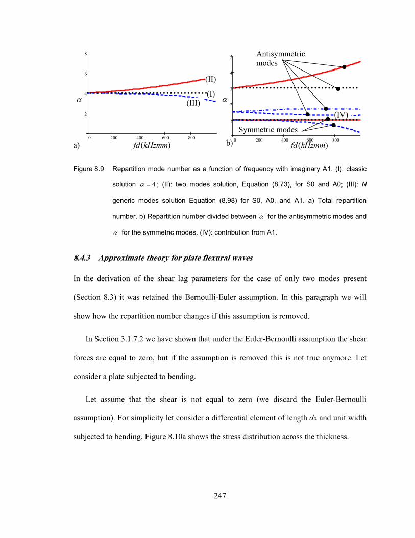
247
Figure 8.9 Repartition mode number as a function of frequency with imaginary A1. (I): classic
solution 4α = ; (II): two modes solution, Equation (8.73), for S0 and A0; (III): N
generic modes solution Equation (8.98) for S0, A0, and A1. a) Total repartition
number. b) Repartition number divided between α for the antisymmetric modes and
α for the symmetric modes. (IV): contribution from A1.
8.4.3 Approximate theory for plate flexural waves
In the derivation of the shear lag parameters for the case of only two modes present
(Section 8.3) it was retained the Bernoulli-Euler assumption. In this paragraph we will
show how the repartition number changes if this assumption is removed.
In Section 3.1.7.2 we have shown that under the Euler-Bernoulli assumption the shear
forces are equal to zero, but if the assumption is removed this is not true anymore. Let
consider a plate subjected to bending.
Let assume that the shear is not equal to zero (we discard the Euler-Bernoulli
assumption). For simplicity let consider a differential element of length dx and unit width
subjected to bending. Figure 8.10a shows the stress distribution across the thickness.
0 200 400 600 800
1
2
3
4
5
α
Antisymmetric modes
α
Symmetric modes 0 200 400 600 800
2
4
6
8
( )fd kHzmm
(I)
(II)
(III)(IV)
a) b) ( )fd kHzmm

248
Figure 8.10 Differential element of length dx. a) normal stress due to bending; b) Shear force
due to the presence of stress.
The stress distribution varies in the x direction; we can assume that after a length dx
the stress is incremented by a quantity xdσ . If we consider an element of length dx and
thickness d y− (Figure 8.10b), the net result of the stress across the thickness is a force F
given by
( )d d
x x x xy yF d dy d dyσ σ σ σ= + − =∫ ∫ (8.118)
Figure 8.11 Forces and moments on a plate. a) Shear stress sign convention. b) Moment
balance.
y
σx σx+d σx
x
dx
F F
τyx
τyx
x
τ(x)
Q
Q M
M+dMb)a)
dx τxy
τxyd-y
d+y
y
d σx σx+d σx
x y
σxσx+d σx
x
dx dx
F F
a) b)
d-y
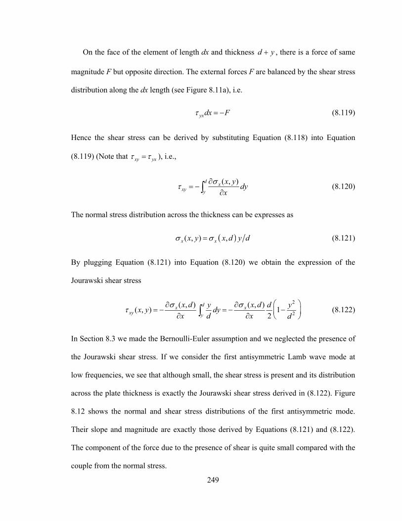
249
On the face of the element of length dx and thickness d y+ , there is a force of same
magnitude F but opposite direction. The external forces F are balanced by the shear stress
distribution along the dx length (see Figure 8.11a), i.e.
yxdx Fτ = − (8.119)
Hence the shear stress can be derived by substituting Equation (8.118) into Equation
(8.119) (Note that xy yxτ τ= ), i.e.,
( , )d xxy y
x y dyx
στ ∂= −
∂∫ (8.120)
The normal stress distribution across the thickness can be expresses as
( )( , ) ,x xx y x d y dσ σ= (8.121)
By plugging Equation (8.121) into Equation (8.120) we obtain the expression of the
Jourawski shear stress
2
2( , ) ( , )( , ) 1
2dx x
xy y
x d x dy d yx y dyx d x d
σ στ⎛ ⎞∂ ∂
= − = − −⎜ ⎟∂ ∂ ⎝ ⎠∫ (8.122)
In Section 8.3 we made the Bernoulli-Euler assumption and we neglected the presence of
the Jourawski shear stress. If we consider the first antisymmetric Lamb wave mode at
low frequencies, we see that although small, the shear stress is present and its distribution
across the plate thickness is exactly the Jourawski shear stress derived in (8.122). Figure
8.12 shows the normal and shear stress distributions of the first antisymmetric mode.
Their slope and magnitude are exactly those derived by Equations (8.121) and (8.122).
The component of the force due to the presence of shear is quite small compared with the
couple from the normal stress.
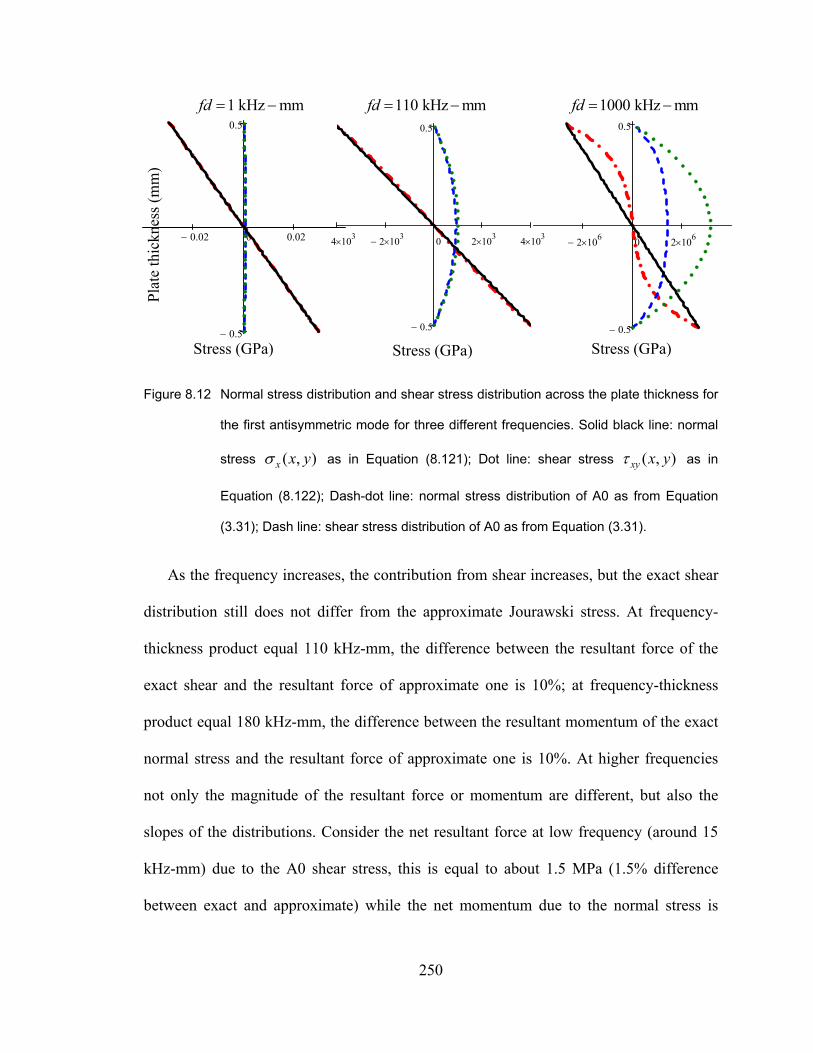
250
Figure 8.12 Normal stress distribution and shear stress distribution across the plate thickness for
the first antisymmetric mode for three different frequencies. Solid black line: normal
stress ( , )x x yσ as in Equation (8.121); Dot line: shear stress ( , )xy x yτ as in
Equation (8.122); Dash-dot line: normal stress distribution of A0 as from Equation
(3.31); Dash line: shear stress distribution of A0 as from Equation (3.31).
As the frequency increases, the contribution from shear increases, but the exact shear
distribution still does not differ from the approximate Jourawski stress. At frequency-
thickness product equal 110 kHz-mm, the difference between the resultant force of the
exact shear and the resultant force of approximate one is 10%; at frequency-thickness
product equal 180 kHz-mm, the difference between the resultant momentum of the exact
normal stress and the resultant force of approximate one is 10%. At higher frequencies
not only the magnitude of the resultant force or momentum are different, but also the
slopes of the distributions. Consider the net resultant force at low frequency (around 15
kHz-mm) due to the A0 shear stress, this is equal to about 1.5 MPa (1.5% difference
between exact and approximate) while the net momentum due to the normal stress is
2− 106× 0 2 106×
0.5−
0.5
4 103× 2− 103× 0 2 103× 4 103×
0.5−
0.5
0.02− 0 0.02
0.5−
0.5
Plat
e th
ickn
ess (
mm
)
Stress (GPa) Stress (GPa) Stress (GPa)
1 kHz mmfd = − 110 kHz mmfd = − 1000 kHz mmfd = −

251
equal to about 2 MPa-mm (0.7% difference between exact and approximate), the two
values are close enough justify the need to remove the Bernoulli-Euler assumption.
To derive the modal repartition number when the Jourawski shear is present, assume
the displacement to be of the form
2
2
( , , )
( , , )
xvu y x z t yx
yv v x z td
ψ ∂⎧ = =⎪ ∂⎪⎨⎪ = −⎪⎩
(8.123)
With this assumption, the shear stress becomes
2
21xyu v v yy x x d
τ μ μ⎛ ⎞∂ ∂ ∂⎛ ⎞= + = −⎜ ⎟⎜ ⎟∂ ∂ ∂ ⎝ ⎠⎝ ⎠
(8.124)
The shear stress resultant is a force in the y direction. This is written as
2
2( , ) ( , )1
2 3
d dx x
x xyd d
x d x dd y tdQ dy dyx xd
σ στ− −
⎛ ⎞∂ ∂= = − − = −⎜ ⎟∂ ∂⎝ ⎠∫ ∫ (8.125)
The normal stress resultant is a net zero force in the x direction and a moment M, i.e.
( ) ( )2
( , ) , ,3
d d
x x x xd d
y tdM x y ydy x d dy x dd
σ σ σ− −
= = =∫ ∫ (8.126)
The moment due to the external force is
( )2tdM x dxτ τ= (8.127)
The balance of the shear force, the bending moment, and the external force due to the
PWAS gives (see Figure 8.11b)
0M dM M Qdx dMτ+ − − + = (8.128)

252
or
0dMdM Qdx dx
τ− + = (8.129)
Substituting Equations (8.125), (8.126), and (8.127) into the equilibrium expression we
obtain
( ), ( , ) ( ) 03 3 2
x xd x d x dtd td t xdx x
σ σ τ∂+ + =
∂ (8.130)
Simplify expression (8.130) to get the final expression
( , ) 3 ( ) 02
x x dt xx
σ τ∂+ =
∂ (8.131)
The shear lag coefficient α is now equal to half the shear lag coefficient without the
Jourawski shear stress.
Procedure above can be generalized for a generic antisymmetric stress distribution
( , , )x x y tσ . The shear force and the moment expressions are respectively:
-
( )( , )( ) ( , )
( )
d d
xd d yx
xydx
y dydyx dQ x x y dyx d
σσσ
σ−∂
= = −∂
∫ ∫∫ (8.132)
( )
( ) ( , ) ( , )( )
d
xdd
z x xxd
y ydyM x x y ydy x d
d
σσ σ
σ−
−
= =∫
∫ (8.133)
Substitution of Equations (8.132) and (8.133) into Equation (8.129), yields

253
2( , ) ( ) ( ) 0
2 ( ) ( )
x xd d
x xd y
x d t dt xx
y y y dy dy
σ σ τσ σ
−
∂+ =
∂ ⎡ ⎤+⎢ ⎥
⎢ ⎥⎣ ⎦∫ ∫
(8.134)
Denote the shear lag parameter as
2 ( )1
2( ) ( )
xd d d
x xd d y
t d
y ydy y dy dy
σασ σ
− −
=⎡ ⎤
+ ⎢ ⎥⎢ ⎥⎣ ⎦
∫ ∫ ∫ (8.135)
Consider the shear stress distribution due to the antisymmetric lamb wave mode, i.e.
( )2 2 2( ) 2 sin( ) 2 sin( )Ax y y D yσ μ ξ β α α ξβ β⎡ ⎤= − + − −⎣ ⎦ (8.136)
The first integral in Equation (8.135) is
2 2 22 sin( )cos( )( ) 2
sin( )2 cos( )
dAx
d
dd dy ydy
dD d d
ξ β α ααα ασ μ
βξ ββ
−
⎡ ⎤+ − ⎛ ⎞−⎜ ⎟⎢ ⎥⎝ ⎠⎢ ⎥=⎢ ⎥⎛ ⎞− −⎢ ⎥⎜ ⎟
⎝ ⎠⎣ ⎦
∫ (8.137)
The shear stress component function of y is
( ) ( )2 2 2 cos( ) cos( )( ) 2 2 cos( ) cos( )d
Ax
y
d yy dy D d yα ασ μ ξ β α ξ β βα−⎡ ⎤= + − − −⎢ ⎥⎣ ⎦∫ (8.138)
With the use of (8.138), the second integral in Equation (8.135) becomes, after
rearrangement
2 2 22 sin( )cos( )( ) 2
sin( )2 cos( )
d dAx
d y
dd dy dydy
dD d d
ξ β α ααα ασ μ
βξ ββ
−
⎡ ⎤+ − ⎛ ⎞−⎜ ⎟⎢ ⎥⎝ ⎠⎢ ⎥=⎢ ⎥⎛ ⎞− −⎢ ⎥⎜ ⎟
⎝ ⎠⎣ ⎦
∫ ∫ (8.139)

254
Note that the two integrals (Equation (8.137) and (8.139)) are equal, i.e.,
( ) ( )d d d
A Ax x
y d y
y ydy y dy dyσ σ−
⎡ ⎤= ⎢ ⎥
⎢ ⎥⎣ ⎦∫ ∫ ∫ (8.140)
Hence Equation (8.134) can be simplified as
( , ) ( ) 0x x dt xx
σ ατ∂+ =
∂ (8.141)
with modal repartition number
2 ( )
4 ( )
xd
xd
t d
y ydy
σασ
−
=
∫ (8.142)
Figure 8.13 shows how the alpha parameter changes with frequency and the effect of
removing the Bernoulli-Euler assumption from derivation in Section 8.3.
Figure 8.13 Repartition mode number due to the A0 mode as a function of frequency. (a): classic
solution with Bernoulli-Euler assumption, 3α = ; (b): 2 modes solution Equation
(8.73) for A0; (c): N generic mode solution Equation (8.98) for A0; (d): 2 modes
solution Equation (8.142) for A0 (normal + shear stress).
α
( )fd kHzmm0 200 400 600 800
1
2
3
4
(a)
(b)
(c)
(d)

255
The repartition mode number with the addition of the shear stress (dash-dot green line)
starts at the low frequencies from 1.5 as derived for the more generic solution (dash blue
line). The repartition number still increases with the frequency as it was found for the
derivation for two modes A0 and S0, but its increment is less than before (before the A1
cut-off frequency the difference in repartition number increment was about 36%). The
discrepancy between the new derivation and the exact for N generic mode lies in the fact
that we assumed that the shear stress distribution is exactly that derived by Jourawski,
beyond fd=110 kHz-mm (solid black vertical line) the force difference between exact and
approximate shear is above 10%, while the difference in repartition number (dash-dot
versus dash line) is of 6%.
8.4.4 Numerical solution of the integral-differential equation
We want to solve the shear stress equilibrium of the bonding layer in the presence of N
wavemodes. Recall the general expression as in Equation (8.101), i.e.
2
1( ) ( ) ( ) ( ) 0n n n n
x aNi x i t i x i t
nn a x
x x i e e t dt e e t dtξ ξ ξ ξτ τ η τ τ− −
= −
⎡ ⎤′′ − Γ − + =⎢ ⎥
⎢ ⎥⎣ ⎦∑ ∫ ∫ (8.143)
with boundary conditions
( )
( )0 0
ISAb
b
a Gt
ετ
τ
⎧ ′ ± =⎪⎨⎪ =⎩
(8.144)
To solve Equation (8.143), we apply the variational iteration method (VIM) as shown in
He (2007) and Wang and He (2007).
The correction functional is

256
2
10
1
( ) ( )
( ) ( ) ( )( ) ( )n n n n
i ixx aN
i i i x i t i x i tn
n a x
s s
x x si e e t dt e e t dtξ ξ ξ ξ
τ τ
τ τ λη τ τ+ − −
= −
⎡ ⎤′′ − Γ −⎢ ⎥
= + ⎛ ⎞⎢ ⎥− +⎜ ⎟⎢ ⎥⎜ ⎟⎢ ⎥⎝ ⎠⎣ ⎦
∫ ∑ ∫ ∫ (8.145)
where iτ% is considered as restricted variations, which means 0iτ =% . λ is a general
Lagrangian multiplier which can be identified optimally via the iteration theory.
First, we find the Lagrangian multiplier by calculating variation with respect to iτ ,
noticing that 0iδτ = , yields
2
10
1
( ) ( )
( ) ( ) ( )( ) ( )n n n n
i ixx aN
i i i x i t i x i tn
n a x
s s
x x s dsi e e t dt e e t dtξ ξ ξ ξ
τ τ
δτ δτ δ λη τ τ+ − −
= −
⎡ ⎤′′ − Γ −⎢ ⎥
= + ⎡ ⎤⎢ ⎥− +⎢ ⎥⎢ ⎥
⎢ ⎥⎢ ⎥⎣ ⎦⎣ ⎦
∫ ∑ ∫ ∫% % (8.146)
or,
21
0
22
20
( ) ( ) ( ) ( ) ( )
( ) ( )( ) ( ) ( ) ( ) ( ) ( )
x
i i i i
x
i i i is xs x
x x s s s ds
d s d sx s s s s s dsds ds
δτ δτ δ λ τ τ
λ λδτ λ δτ δτ λ δτ
+
==
⎡ ⎤′′= + − Γ⎣ ⎦
⎡ ⎤′= + − + − Γ⎢ ⎥
⎣ ⎦
∫
∫ (8.147)
We obtain the following stationary conditions:
22
2( , ) ( , ) 0
( , )1 0
( , ) 0s x
s x
d x s x sdsd x s
dsx s
λ λ
λ
λ=
=
⎧− Γ =⎪
⎪⎪
− =⎨⎪⎪ =⎪⎩
(8.148)
Solve the above differential equation to find the Lagrange multiplier. The general
solution is

257
( , ) sinh ( ) cosh ( )x s A s x B s xλ = Γ − + Γ − (8.149)
Applying the boundary conditions yields
( , ) 0
( , ) cosh ( ) 1
x x Bd x x A s x
ds
λλ
= =⎧⎪⎨
= Γ Γ − =⎪⎩
(8.150)
hence, rearranging the terms
1
0
A
B
⎧ =⎪Γ⎨
⎪ =⎩
(8.151)
Finally we obtain the Lagrangian multiplier
sinh ( )( , ) s xx sλ Γ −=
Γ (8.152)
Substitute Equation (8.152) into Equation (8.145), for simplicity let consider the presence
of one wavemode only, we obtain the following iteration formula
2
10
1
( ) ( )sinh ( )( ) ( )
( ) ( )n n n n
i ixx aN
i i i x i t i x i tn
n a x
s ss xx x ds
i e e t dt e e t dtξ ξ ξ ξ
τ τ
τ τη τ τ+ − −
= −
⎡ ⎤′′ − Γ⎢ ⎥Γ −
= + ⎡ ⎤⎢ ⎥Γ − +⎢ ⎥⎢ ⎥
⎢ ⎥⎢ ⎥⎣ ⎦⎣ ⎦
∫ ∑ ∫ ∫% %(8.153)
Assume that the approximate solution to be of the type
0 ( ) sinhx A xτ = Γ (8.154)
Substitute the approximate solution in the iteration formula and rearrange the terms to
obtain, i.e.,

258
11 0
sinh
( ) sinh sinh ( )
sinh
n n
n
si s i t
xNa
n an i s i t
s
e e tdtiAx A x s x ds
e e tdt
ξ ξ
ξ ξ
τ η
−
−
= −
⎡ ⎤Γ⎢ ⎥
⎢ ⎥= Γ − Γ − ⎢ ⎥Γ ⎢ ⎥+ Γ⎢ ⎥⎣ ⎦
∫∑ ∫
∫ (8.155)
Solve the integral in dt in Equation (8.155) and substitute the result in the original
equation to get
1
1 0
( ) sinh
sinh ( )2
s s a i a a i ai s
xN
n a i a a i a s sn i s
x A x
e e e eei i i iiA s x ds
e e e eei i i i
ξ ξξ
ξ ξξ
τ
ξ ξ ξ ξη
ξ ξ ξ ξ
Γ −Γ −Γ − Γ −−
Γ − −Γ − Γ −Γ=
= Γ
⎡ ⎤⎛ ⎞+ − +⎢ ⎥⎜ ⎟Γ + Γ − Γ + Γ −⎝ ⎠⎢ ⎥− Γ − ⎢ ⎥Γ ⎛ ⎞⎢ ⎥+ + − −⎜ ⎟⎢ ⎥Γ − Γ + Γ − Γ +⎝ ⎠⎣ ⎦
∑ ∫ (8.156)
Solve the integral in ds in Equation (8.156), after rearrangement we get
( ) ( ) ( )
( ) ( )
1
2 2 2 22 2
1
2 2 2 2 2 2
( ) sinh
2 sinhsinh
2 cosh cosh2 sin
a ai a
N
n a an i a
x A x
i e e ax ei iAi
x x a e ei ie xi i
ξ
ξ
τ
ξξξ ξ ξ
η
ξ ξξ ξ ξ ξ
Γ −Γ−
Γ −Γ= −
= Γ
⎧ ⎫⎡ ⎤⎛ ⎞ΓΓ − − − −⎪ ⎪⎢ ⎥⎜ ⎟⎜ ⎟Γ +Γ Γ + Γ − Γ +⎪ ⎪⎢ ⎥⎪ ⎝ ⎠ ⎪⎣ ⎦− ⎨ ⎬Γ ⎛ ⎞Γ Γ⎪ ⎪+ + + +⎜ ⎟⎪ ⎪⎜ ⎟Γ + Γ + Γ − Γ +⎪ ⎪⎝ ⎠⎩ ⎭
∑ (8.157)
This is the first approximate solution. Let’s apply the boundary conditions to derive
constant A. First derivative Equation (8.157) with respect to x, i.e.,
( ) ( ) ( )
( ) ( )
1
2 2 2 22 2
2 21
2 2 2 2
( ) cosh
2 sinhcosh
cosh sinh22
coshcos
a ai a
N
nn
a ai a
x A x
i e e ax ei i
Ai x x xi
a e ei e xi i
ξ
ξ
τ
ξξξ ξ ξ
η η ξξ
ξ ξξ ξ ξ
Γ −Γ−
=
Γ −Γ−
′ = Γ Γ
⎧ ⎫⎡ ⎤⎛ ⎞ΓΓ Γ − − − −⎪ ⎪⎢ ⎥⎜ ⎟⎜ ⎟Γ +Γ Γ + Γ − Γ +⎪ ⎪⎢ ⎥⎝ ⎠⎣ ⎦
⎪ ⎪Γ + Γ Γ⎪ ⎪− +⎨ ⎬
Γ Γ +⎪ ⎪⎪ ⎪⎛ ⎞Γ⎪ ⎪+ + +⎜ ⎟⎜ ⎟⎪ ⎪Γ + Γ − Γ +⎝ ⎠⎩ ⎭
∑ (8.158)

259
Apply the boundary conditions (8.144), i.e.,
( ) ( ) ( )
( ) ( )
1
2 2 2 22 2
2 21
2 2 2 2
( ) cosh
2 sinhcosh
cosh sinh22
coshcos
a ai a
N
nn
a ai a
b IS
a A a
i e e aa ei i
iA a a ai
a e ei e ai i
G
ξ
ξ
τ
ξξξ ξ ξ
η ξξ
ξ ξξ ξ ξ
ε
Γ −Γ−
=
Γ −Γ−
′ ± = Γ Γ
⎧ ⎫⎡ ⎤⎛ ⎞Γ−Γ Γ + − −⎪ ⎪⎢ ⎥⎜ ⎟⎜ ⎟Γ +Γ Γ + Γ − Γ +⎪ ⎪⎢ ⎥⎝ ⎠⎣ ⎦
⎪ ⎪Γ + Γ Γ⎪ ⎪− +⎨ ⎬
Γ Γ +⎪ ⎪⎪ ⎪⎛ ⎞Γ⎪ ⎪+ + +⎜ ⎟⎜ ⎟⎪ ⎪Γ + Γ − Γ +⎝ ⎠⎩ ⎭
=
∑
A
bt
(8.159)
Solution of Equation (8.159) yields
b ISA
b
GAt Qε
= (8.160)
where
( ) ( ) ( )
( ) ( )
2 2 2 22 2
2 21
2 2 2 2
cosh
2 sinhcosh
cosh sinh22
coshcos
a ai a
N
nn
a ai a
Q a
i e e aa ei i
i a a ai
a e ei e ai i
ξ
ξ
ξξξ ξ ξ
η ξξ
ξ ξξ ξ ξ
Γ −Γ−
=
Γ −Γ−
= Γ Γ
⎧ ⎫⎡ ⎤⎛ ⎞Γ−Γ Γ + − −⎪ ⎪⎢ ⎥⎜ ⎟⎜ ⎟Γ +Γ Γ + Γ − Γ +⎪ ⎪⎢ ⎥⎝ ⎠⎣ ⎦
⎪ ⎪Γ + Γ Γ⎪ ⎪− +⎨ ⎬
Γ Γ +⎪ ⎪⎪ ⎪⎛ ⎞Γ⎪ ⎪+ + +⎜ ⎟⎜ ⎟⎪ ⎪Γ + Γ − Γ +⎝ ⎠⎩ ⎭
∑ (8.161)
Hence the first iteration is written as

260
( ) ( ) ( )
( ) ( )
1
2 2 2 22 2
1
2 2 2 2 2 2
( ) sinh
2 sinhsinh
2 cosh cosh2 sin
b ISA
b
a ai a
Nb ISA
n a anb i a
Gx xt Q
i e e ax ei iGi
t Q x x a e ei ie xi i
ξ
ξ
ετ
ξξξ ξ ξε η
ξ ξξ ξ ξ ξ
Γ −Γ−
Γ −Γ= −
= Γ
⎧ ⎫⎡ ⎤⎛ ⎞ΓΓ − − − −⎪ ⎪⎢ ⎥⎜ ⎟⎜ ⎟Γ +Γ Γ + Γ − Γ +⎪ ⎪⎢ ⎥⎪ ⎝ ⎠ ⎪⎣ ⎦− ⎨ ⎬Γ ⎛ ⎞Γ Γ⎪ ⎪+ + + +⎜ ⎟⎪ ⎪⎜ ⎟Γ + Γ + Γ − Γ +⎪ ⎪⎝ ⎠⎩ ⎭
∑ (8.162)
Note that for 0bt → , i.e., aΓ → ∞ , Equation (8.162) becomes
( )
31
2 sinh sinhlim cosh 1 cosh2 cos2 2
i aN
n i aa n
i e a aQ a i ai e ai a
ξ
ξ
ξη
ξ ξξ
−
−Γ →∞ =
⎧ ⎫⎡ ⎤− − Γ − Γ⎪ ⎪⎢ ⎥≈ Γ Γ − ≈ Γ Γ⎨ ⎬⎢ ⎥Γ + +⎪ ⎪⎢ ⎥Γ⎣ ⎦⎩ ⎭
∑ (8.163)
and the interfacial shear stress becomes
( )
1
4
lim ( ) sinhcosh
sinh 2 sinh sinhcosh
2
b ISAa b
i a
b ISAn
b
Gx xt a
x i e a aG ait
ξ
ετ
ξε η
Γ →∞
−
≈ ΓΓ Γ
Γ− − Γ − Γ
Γ Γ−Γ 1 cosh2 2 sin
cosh
N
n i axi x ie xa
ξξ ξ= −
⎧ ⎫⎡ ⎤⎪ ⎪⎢ ⎥⎪ ⎪⎣ ⎦⎨ ⎬
Γ⎪ ⎪+ +⎪ ⎪Γ⎩ ⎭
∑ (8.164)
With the use of the shear lag definition in Equation (8.31) and Equation (8.46), the
interfacial shear stress simplifies as
( ) ( )[ ]1 0sinhlim ( )cosh
aa ISAa
t xx E a x a x aa a
ψτ ε τ δ δα ψΓ →∞
Γ≈ Γ ≈ − − +
+ Γ (8.165)
This is the expression of the shear stress under ideal bond assumption.
8.5 STRESS DISTRIBUTION IN THE BONDING LAYER
The effect of the adhesive, actuator, and structure parameters on the shear stress
distribution have been extensively discussed in Section 8.2.1. In this Section, we focus on

261
the difference in shear stress transferred between the derivation for low frequencies
approximation, Equation (8.44), and that for N generic modes, Equation (8.162).
Figure 8.14a shows how the shear stress transferred by the PWAS to the structure
varies with frequency. Lines I and II are the shear stress distribution as derived from
Equation (8.44) and from Equation (8.162) for fd=1 kHz-mm. The difference between the
two curves is due to the different values in the modal repartition number. As fd increases,
the shear stress curves shifts down till it reaches the cut-off frequency (line III). After the
cut-off frequency, the shear stress is closer to the approximate solution (lines I and IV
respectively) and then it continues to shift downwards as the fd product increases.
Figure 8.14b shows the percentage difference between the two equations in load
transmitted for different frequency values (gray area in Figure 8.14a). At low frequencies,
the difference is about 14%, this difference is entirely due to the different modal
repartition number at low frequencies (4 vs. 2.5). If we use the value of 2.5 for α in the
low frequencies approximation, the two curves (I and II) become identical. As the
frequency increases, the percentage of PWAS length used to transfer the load does not
change but the amount of load transferred increases linearly till the first cut-off frequency
(fd-~800 kHz-mm) up to 20%. Figure 8.14b shows that beyond the first cut-off
frequency, (A1 is propagating), there is a sudden discontinuity that reflects the
discontinuity in the derivation of the modal repartition number. The percentage difference
drops to 3% and than it start to increase again with the same curvature.

262
Figure 8.14 Shear stress variation with frequency. a) Shear stress transmitted by the PWAS to
the structure through a bond layer. (I): shear stress derived for low frequency
approximation ( 4α = ), Equation (8.44); All other curves: shear stress derived in the
generic N mode formulation ( fα = (frequency,no. of modes)), Equation (8.162). (II)
fd=1 kHz-mm; (III) fd=783 kHz-mm before the cut-off frequency; (IV) fd=784 kHz-mm
after the cut-off frequency). b) Percentage difference in load transmitted at different
frequency-thickness products.
Figure 8.15a shows the change in shear stress transfer with frequency when the
imaginary branch of A1 is considered. There is no significant difference in the shear
curves for different derivation methods and different frequencies.
Figure 8.15b shows that there is no discontinuity at the cut-off frequency and the total
load transferred from the actuator to the structure increases till 8% in the frequency-
thickness range 0-1000 kHz-mm.
(I)
(II)
Perc
enta
ge
diff
eren
ce
oftra
nsm
itted
load
( )fd kHzmm
( )xτ
2·Area = transmitted load
a) b) 0 200 400 600 800
5
10
15
20
(III) (IV)
x a

263
Figure 8.15 Interfacial shear stress distribution and percentage of change a) Shear stress
transmitted by the PWAS to the structure through a bond layer with imaginary A1.
(I): shear stress derived for low frequency approximation ( 4α = ); (II): shear stress
derived in the generic N mode formulation ( fα = (frequency, no. of modes)) for
different frequencies (fd=1; 200; 781; 850 (solid line); 1000 kHz-mm (dash-dot ]
line)). b) Percentage difference in load transmitted at different frequency-thickness
products.
Perc
enta
ge
diff
eren
ce
oftra
nsm
itted
load
( )fd kHzmm
( )xτ
x a
2·Area = transmitted load
a) b)
(I)
(II) 0 200 400 600 800
10
20

264
9 TUNED GUIDED WAVES EXCITED BY PWAS
This section deals with the aspect of the interaction between PWAS and structure during
the active SHM process, i.e., tuning between the PWAS and the Lamb waves traveling in
the structure. The PWAS, under electric excitation, transfers the oscillatory contractions
and expansion to the bonded layer and the layer to the metal surface. In this process
several factors influences the wave behavior: thickness of the bonding layer, geometry of
the PWAS, thickness and material of the plate. The result of the influence of all these
factors is the tuning of the PWAS with the material. This phenomenon has been studied
recently by Giurgiutiu (2005) who developed the theory of the interaction of the PWAS
with the structure for a rectangular PWAS with an infinite dimension. Lately Raghavan
and Cesnik (2004) extended these results to the case of a circular transducer.
In the first part of this section, we present the different models to represent the load
transferred from the PWAS to the structure through a bond layer. First we consider the
simple case of ideal bonding solution which permits the use of the pin-force model. Then
we present the case in which the bond layer has a finite thickness. The load transfer
models are used to derive the theoretical tuning curves. We show that the same
theoretical curves can be obtained through the Fourier transformation method as derived
by Giurgituiu (2005) and through the NME method presented in the present dissertation.
Let’s consider the excitation provided by a PWAS bonded through an adhesive layer
to the top surface of a plate. The excitation can be modeled in different ways. Hereunder,

265
we report first the case of ideal bonding solution in which we assume the bonding layer to
be small; second the case in which the bonding layer can assume different thickness but
we retain the low frequency approximation of the shear lag; finally, we will show the
case of non ideal bonding conditions under the shear lag exact solution.
9.1 SHEAR TRANSFER THROUGH BOND LAYER
9.1.1 Ideal bond solution
Assume the PWAS to be attached to the structure ideally, hence assume ideal bond. The
shear stress transfer takes place into an infinitesimal regions at the PWAS tips, i.e.,
( ) ( )0 if
( , )0 if
x
x a x a x at x d
x a
τ δ δ⎧ − − + ≤⎡ ⎤⎪ ⎣ ⎦= ⎨>⎪⎩
(9.1)
where 0a
a ISAt Ea
ψτ εα ψ
=+
. Substituting (9.1) into the expression of the filed amplitude,
Equation (7.125), we obtain:
( ) ( )0( )( )
4n n
ani x i xx
nnn a
v da x e x a x a e dxP
ξ ξτ δ δ−+
−
= − − +⎡ ⎤⎣ ⎦∫%
(9.2)
In Equation (9.2) the term 0τ depends on the excitation, term ( )4
nx
nn
v dP
% is the excitability
function of mode n (depends on the mode excited and not on the source used for
excitation), and term
( ) ( ) n
ai x
na
F x a x a e dxξδ δ−
= − − +⎡ ⎤⎣ ⎦∫ . (9.3)
is the Fourier integral. Its solution is

266
( ) ( ) ( ) ( )
2 sin
n n n
n n
a a ai x i x i x
na a a
i a i an
F x a x a e dx x a e dx x a e dx
e e i a
ξ ξ ξ
ξ ξ
δ δ δ δ
ξ− − −
−
= − − + = − − +⎡ ⎤⎣ ⎦
= − =
∫ ∫ ∫ (9.4)
Substitute this value in Equation (9.2) to obtain
0( )( ) sin2
ni xnx
n nnn
v d ea x i aP
ξ
τ ξ−
+ = −%
(9.5)
Equation (9.5) represents the PWAS-Lamb wave tuning amplitude for ideal bonding
conditions.
9.1.2 Shear-lag stress excitation with low frequency approximation
Consider the excitation provided by a PWAS. If we describe this phenomenon through
the shear lag model, the shear stress in the bonding layer is assumed of the form, see
Equation (8.59),
1 sinh if ( , )
0 if x
x x at x d
x a
τ⎧ Γ ≤⎪= ⎨>⎪⎩
(9.6)
where 1 0 cosha
aτ τ Γ
=Γ
. Substituting Equation (9.6) into Equation (7.125) we obtain
( )1( )( ) sinh
4n n
ani x i xx
nnn a
v da x e x e dxP
ξ ξτ −
−
= Γ∫%
(9.7)
where the Fourier integral ( )n nF ξ is a tuning function that depends on the relation
between the PWAS size, 2a , and the modal wavenumber, nξ , i.e.,
( ) ( )sinh n
ai x
n na
F x e dxξξ−
= Γ∫ for a x< (9.8)

267
Integral (9.8) can be solved explicitly to get
( ) 2 2
sin cosh sinh cos2 n n nn n
n
a a a aF i ξ ξ ξξξ
Γ Γ − Γ=
Γ + (9.9)
Substituting Equation (9.9) into Equation (9.7) yields
1 2 2
( ) sin cosh sinh cos( )2
ni xnx n n n
nnn n
v d e a a a aa x iP
ξ ξ ξ ξτξ
−+ Γ Γ − Γ
=Γ +
% (9.10)
For the shear lag case we provide the complete solution, hence solution for x<a. as in
Equation (7.123). Note that, for the domain a x a− ≤ ≤ , i.e., under the PWAS, the
function nF takes the form
( ) ( ), sinh n
xi x
n na
F x x e dxξξ−
= Γ∫ for a x a− ≤ ≤ (9.11)
Upon integration, Equation (9.11) becomes
( ) ( )( ) ( )1, sinh
2
n nn
xx x i x ii x
n nn na a
e eF x x e dxi i
ξ ξξξ
ξ ξ
Γ+ − Γ−
− −
⎡ ⎤= Γ = +⎢ ⎥Γ + Γ −⎣ ⎦
∫ (9.12)
Processing of Equation (9.12) gives the closed-form solution
( )( ) ( ) ( ) ( )1,
2
n n n nx i a i x i a i
n nn n
e e e eF xi i
ξ ξ ξ ξ
ξξ ξ
Γ+ − Γ+ − Γ− Γ−⎡ ⎤− −= +⎢ ⎥Γ + Γ −⎣ ⎦
(9.13)
Substituting Equation (9.13) into Equation (7.123) for the case of wave propagation
inside the excitation region, gives
( ) ( ) ( ) ( )
1( )( ) for 8
n n n nn x i a i x i a ii xnx
nnn n n
v d e e e e ea x a x aP i i
ξ ξ ξ ξξ
τξ ξ
Γ+ − Γ+ − Γ− Γ−−+ ⎡ ⎤− −
= + − ≤ ≤⎢ ⎥Γ + Γ −⎣ ⎦
%(9.14)

268
Similarly, we can develop closed-form solutions for the backward wave. Substituting
Equation (9.6) into Equation (7.124) for x a< − , gives
( )1( )( ) sinh
4n n
ani x i xx
nnn a
v da x e x e dxP
ξ ξτ −−
−
= Γ∫%
(9.15)
The tuning function for the backward wave is defined as
( ) ( )sinh n
ai x
n na
F x e dxξξ −
−
= Γ∫ for a x> (9.16)
Integral (9.16) can be solved explicitly and becomes after rearrangement
( ) 2 2
cos sinh sin cosh2 n n nn n
n
a a a aF i ξ ξ ξξξ
Γ − Γ Γ=
Γ + (9.17)
Substituting Equation (9.17) into Equation (9.15) yields
1 2 2
( ) sinh cos cosh sin( )2
ni xnx n n n
nnn n
v d e a a a aa x iP
ξ ξ ξ ξτξ
− Γ − Γ Γ= −
Γ +%
(9.18)
For backward wave in the domain a x a− ≤ ≤ , i.e., under the PWAS, the function nF
takes the form
( ) ( ), sin n
ai x
n nx
F x x e dxξξ −= Γ∫ for a x a− ≤ ≤ (9.19)
Upon integration, Equation (9.11) becomes
( ) ( ) ( ) ( )( ) ( )1 1, sin
2 2
n nn nn
aa a x i x ix i x ii x
n nn nx x x
e eF x x e dx e e dxi i
ξ ξξ ξξξ
ξ ξ
Γ− − Γ+Γ− − Γ+− ⎡ ⎤
⎡ ⎤= Γ = − = +⎢ ⎥⎣ ⎦ Γ − Γ +⎣ ⎦∫ ∫ (9.20)
Processing of Equation (9.12) gives the closed-form solution

269
( )( ) ( ) ( ) ( )1,
2
n n n na i x i a i x i
n nn n
e e e eF xi i
ξ ξ ξ ξ
ξξ ξ
Γ− Γ− − Γ+ − Γ+⎡ ⎤− −= +⎢ ⎥Γ − Γ +⎣ ⎦
(9.21)
Note that the ideal bonding solution is the limit case of the shear lag solution as Γ goes
to infinity. To prove it, take the limit of Equation (9.10) for Γ → ∞ , i.e.,
( )2 2
( ) sin cosh sinh coslim ( ) lim2 cosh
ni xna a ISA x n n n
na ann n
t E v d e a a a aa x i aa P a
ξε ξ ξ ξψα ψ ξ
−+
Γ →∞ Γ →∞
Γ Γ − Γ= Γ
+ Γ + Γ%
(9.22)
since ( )( )2
sinhlim 0
cosha
aΓ→∞
Γ=
Γ Γ, hence Equation (9.22) becomes
0( ) ( )lim ( ) sin sin2 2
n ni x i xn na x x
n a ISA n nann nn
t v d e v d ea x i E a a ia aa P P
ξ ξψ ε ξ τ ξα ψ
− −+
Γ →∞= =
+% %
(9.23)
This is the same expression derived for forward propagating modes exited by a PWAS
ideally bonded on the top surface of a plate as in Equation (9.5).
9.1.3 Shear-lag stress excitation for N generic modes
Consider the shear stress in the bonding layer as derived for N generic modes, Equation
(8.162). Substitution of Equation (8.162) into Equation (7.74) yields
( )
( ) ( )
( )
2 22 2
12 2
2 2 2 2
2
2 sinh
1 sinh2
( ) cosh cosh2 sin
2 sin
n
n
n
n
i an
N nnna a
n i a
n n
b ISAx i a
b n nn nn
a ai a
nn
i aei x
e eei i
Gt x x x at Q e x
e ee xi
ξ
ξ
ξ
ξ
ξξξη
ξ ξε
ξ ξξ ξη
ξξ
−
Γ −Γ= −
−
Γ −Γ−
⎧ ⎫Γ⎡ ⎤− +⎪ ⎪⎢ ⎥Γ +Γ Γ +⎪ ⎪⎢ ⎥− Γ⎨ ⎬⎢ ⎥⎛ ⎞Γ⎪ ⎪⎢ ⎥− −⎜ ⎟⎜ ⎟⎪ ⎪Γ − Γ +⎢ ⎥⎝ ⎠⎣ ⎦⎩ ⎭= Γ Γ
+Γ + Γ +
+Γ + +
Γ −
∑
( )1
2
0
N
n
n
x a
i
otherwise
ξ=
⎧⎪⎪⎪⎪⎪⎪ ≤⎪⎨ ⎡ ⎤⎪ ⎢ ⎥⎪ ⎢ ⎥⎪ ⎢ ⎥⎛ ⎞⎪ ⎢ ⎥⎜ ⎟⎜ ⎟Γ +⎪ ⎢ ⎥⎝ ⎠⎣ ⎦⎪⎪⎩
∑
(9.24)
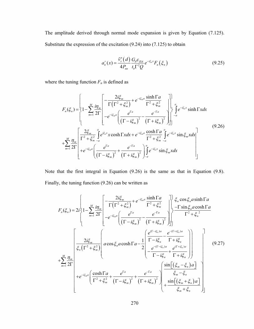
270
The amplitude derived through normal mode expansion is given by Equation (7.125).
Substitute the expression of the excitation (9.24) into (7.125) to obtain
( ) ( )2( )4
n
ni xx b ISA
n n nnn b
v d Ga x e FP t Q
ξε ξ−+ =Γ
% (9.25)
where the tuning function Fn is defined as
( )
( ) ( )
2 22 2
12 2
2 2 2 2
2 sinh
( ) 1 sinh2
2 coshcosh sin
2
m
n
m
n m n
i am
aM mm i xmn n a a
m i a a
m m
a ai x i a i xm
mm ma am
i aeiF e xdx
e eei i
ae x xdx e e xdx
ξ
ξ
ξ
ξ ξ ξ
ξξξηξ
ξ ξ
ξ ξξ ξη
−
−Γ −Γ
= − −
− −
− −
⎧ ⎫Γ⎡ ⎤− +⎪ ⎪⎢ ⎥Γ +Γ Γ +⎪ ⎪⎢ ⎥= − Γ⎨ ⎬⎢ ⎥⎛ ⎞Γ⎪ ⎪⎢ ⎥− −⎜ ⎟⎜ ⎟⎪ ⎪Γ − Γ +⎢ ⎥⎝ ⎠⎣ ⎦⎩ ⎭
ΓΓ +
Γ + Γ ++
Γ
∑ ∫
∫ ∫
( ) ( )1
2 2 sinm n
M
aa am i a i x
mam m
e ee e xdxi i
ξ ξ ξξ ξ
Γ −Γ= − −
−
⎡ ⎤⎢ ⎥⎢ ⎥⎢ ⎥⎛ ⎞⎢ ⎥+ +⎜ ⎟⎜ ⎟⎢ ⎥Γ − Γ +⎝ ⎠⎣ ⎦
∑∫
(9.26)
Note that the first integral in Equation (9.26) is the same as that in Equation (9.8).
Finally, the tuning function (9.26) can be written as
( )
( ) ( )
( )
2 22 2
2 21
2 2
( ) (
2 2
2 sinh cos sinhsin cosh( ) 2 1
2
2 1cos cosh2
2
m
m
n
i am n nM mmm n
n n a am i a n
m m
i a
nmn
n m
m
i a a aei a aF i
e eei i
e eii a a a
ξ
ξ
ξ
ξ ξ ξξξη ξξ
ξξ ξ
ξξ ξξ ξ
η
−
Γ −Γ= −
Γ− −
⎧ ⎫Γ⎡ ⎤ Γ− +⎪ ⎪⎢ ⎥Γ +Γ Γ + −Γ Γ⎪ ⎪⎢ ⎥= −⎨ ⎬⎢ ⎥⎛ ⎞Γ Γ +⎪ ⎪⎢ ⎥− −⎜ ⎟⎜ ⎟⎪ ⎪Γ − Γ +⎢ ⎥⎝ ⎠⎣ ⎦⎩ ⎭
−Γ −
Γ −Γ +
+Γ
∑
( ) ( )
( )
( )
)
( ) ( )
2 22 2
sin
coshsin
n
n n
m
i a
ni a i a
n n
m m n
a am ni a
m m m m n
m n
i
e ei i
a
a e eei i a
ξ
ξ ξ
ξ
ξ
ξ ξ
ξ ξξ ξ
ξ ξ ξ ξ ξξ ξ
Γ+
− Γ− Γ+
=
Γ −Γ−
⎡ ⎤⎛ ⎞⎛ ⎞⎢ ⎥⎜ ⎟⎜ ⎟Γ +⎢ ⎥⎜ ⎟⎜ ⎟⎢ ⎥⎜ ⎟⎜ ⎟⎢ ⎥⎜ ⎟− +⎜ ⎟⎜ ⎟⎜ ⎟Γ − Γ +⎢ ⎥⎝ ⎠⎝ ⎠⎢ ⎥
⎛ ⎞−⎡ ⎤⎢ ⎥⎣ ⎦⎜ ⎟⎢ ⎥−⎛ ⎞Γ ⎜ ⎟⎢ ⎥+ + +⎜ ⎟⎜ ⎟⎢ ⎥⎜ ⎟Γ + Γ − Γ + +⎡ ⎤⎝ ⎠ ⎣ ⎦⎜ ⎟⎢ ⎥+⎜ ⎟+⎢ ⎥⎝ ⎠⎣ ⎦
1
M
∑
(9.27)

271
9.2 PWAS – LAMB WAVES TUNING
The tuning between structure and PWAS is the selective Lamb mode excitation with
PWAS transducer. Under electric excitation, the PWAS undergoes oscillatory
contractions and expansions which are transferred to the structure through the bonding
layer and thus excite Lamb waves into the structure. In this process, several factors
influence the behavior of the excited wave: the thickness of the bonding layer, the
geometry of the PWAS, the thickness and material of the structure. The result of the
influence of all these factors is the tuning of the PWAS with various Lamb wave modes
in the material. Figure 9.1 shows the coupling between PWAS and two Lamb wave
modes, S0 and A0. Maximum coupling between PWAS and the Lamb mode happens
when the PWAS length is an odd multiple of half the wavelength λ . Since different
wave modes have different wavelengths, which vary with frequency, the opportunity
arises for selectively exciting various Lamb modes at various frequencies.
This phenomenon has been studied by Giurgiutiu (2003) who developed the theory of
the interaction of a rectangular PWAS with straight-crested Lamb waves. Lately,
Raghavan and Cesnik (2004) extended these results to the case of a circular transducer
coupled with circular-crested Lamb waves. Both methods were developed through the
Fourier integral transformation of the wave fields. In this section, we will apply a novel
method to obtain the tuning curves, i.e., normal mode expansion model. We will show
numerically that there is no difference between the two formulations. However, a
theoretical proof is provided in the Appendix F.

272
Figure 9.1 S0 and A0 particle displacement and interaction of PWAS with Lamb waves. (Bao
2003)
To obtain the tuning curves we must derive the strain in the structure. The strain in the
structure due to the excitation is given by
( , , )xx x
u v x y t dtx x
ε ∂ ∂= =
∂ ∂ ∫ (9.28)
Recall the expression of velocity derived through normal mode expansion in Equation
(7.126), hence the expression of the strain becomes
1( ) ( ) ( ) ( )i t i tx n x n n x
n na x v y e dt a x v y e
xω ωε ξ
ω− −∂
= =∂ ∑ ∑∫ (9.29)
or in expanded form using Equation (9.5)
h
= 2
d
λ/2
V(t)PWAS ~
V(t)PWAS ~
λ/2
h =
2d
S0
A0

273
( ) ( )0
( ) ( ) sin2
ni x tx nxx n n
n nn
v y v dia a eP
ξ ωε τ ξ ξω
−= ∑%%
(9.30)
This represents the tuning expression of the strain in the structure excited by the PWAS
under the ideal bonding conditions. The tuning expression for the strain was derived by
Giurgiutiu (2003) through Fourier transformation method, i.e.,
( ) ( )( ) ( ) ( )0
', sin ni x tn nx n
n n n
Nax t a eD
ξ ωξτε ξμ ξ
−= − ∑%
(9.31)
Where nD′ is the derivate with respect to the wavenumber of the Rayleigh-Lamb
equation, ( )2 2 cos cosnN d dξβ ξ β α β= + for antisymmetric modes and
( )2 2 sin sinnN d dξβ ξ β α β= + for symmetric modes. In Appendix F we prove
analytically that the expression of the strain derived through normal mode expansion is
the same as that derived with the Fourier transformation.
0 1000 2000 3000 4000 5000 6000
0.02
0.04
0.06
0.08
0.1
0.12
0.14
0.16Modal expansionFourier transformationModal expansionFourier transformation
Symmetric mode
f (kHz)
Stra
in
0 1000 2000 3000 4000 5000 6000
0.02
0.04
0.06
0.08
0.1
0.12
Modal expansionFourier transformationModal expansionFourier transformation
Antisymmetric mode
f (kHz)
Stra
in
Figure 9.2 Comparison of tuning curves for the strain excited by a PWAS derived through the
Fourier transformation model and the normal mode expansion method.

274
Figure 9.2 shows the numerical derivation of the strain for S0 and A0 modes. The solid
lines are the strain values calculated with Equation (9.30), the dotted lines are the strain
values calculated with Equation (9.31). The two derivations are identical
9.2.1 Experimental results and theoretical predictions
Pitch-catch experiments were performed in which one PWAS served as transmitter and
another PWAS served as receiver. The predicted values of the tuning curves were
compared with the experimental results. The signal used in the experiments was a
Hanning-windowed tone burst with 3 counts. The signal was generated with a function
generator (Hewlett Packard 33120A) and sent through an amplifier (Krohn-Hite model
7602) to the transmitter PWAS. A data acquisition instrument (Tektronix TDS5034B)
was used to measure the signal from the receiver PWAS. Several plates were used in the
experiments: (1) aluminum alloy 2024-T3 with 1-mm thickness and 1200x1060-mm size;
(2) aluminum alloy 6061-T8 with 3-mm thickness and 500×500-mm size; (3) aluminum
alloy 2024-T3 with 3-mm thickness and 1200×1200-mm size. In each experiment, we
used a pair of PWAS at a distance of 250 mm from one another. The frequency of the
signal was swept from 10 to 700 kHz in steps of 20 kHz. At each frequency, we collected
the wave amplitude and the time of flight for both the symmetric mode and the
antisymmetric modes.
9.2.1.1 Square PWAS
Square PWAS 7-mm long, 0.2-mm thick (American Piezo Ceramics APC-850) were
used on two aluminum 2024-T3 plates of different thickness (1 mm and 3 mm) and one
aluminum 6061-T8 plate of 3-mm thickness.

275
9.2.1.1.1 Experiments on 2024-T3 plate with 1-mm thickness and 1200×1060-mm size
Figure 9.3 shows the configuration for the square PWAS on the 2024-T3 aluminum alloy
plate 1-mm thick. The PWAS were located at the center of the plate in order to avoid
interference with the reflection from the boundaries.
Figure 9.3 Aluminum plate 2024-T3 1-mm thick with square, rectangular and round PWAS
The group velocities of the S0 mode were detected with no difficulties at each
frequency. The A0 mode was followed closely at each frequency, but, for frequencies
where the wave amplitude was closer to zero, the experimental values were more distant
from the predicted values. Figure 9.4 shows the experimental data (cresses and circles)
and predicted values (solid lines) of the wave amplitude for the S0 and A0 modes. For the
theoretical predictions, we used an effective PWAS length of 6.4 mm. For this effective
PWAS length value, we obtain the best agreement between experiments and predictions.
In the development of the theory, it was assumed that there was ideal bonding between
the PWAS and the plate. This assumption means that the stresses between the transducers
and the plate are fully transferred at the PWAS ends. In reality, the stresses are
transferred over a region adjacent to the PWAS ends (Figure 8.3).
P1
1200 mm
1200
mm
250mm 250mm
250mm
P
P2

276
Figure 9.4 Tuning for aluminum 2024-T3, 1-mm thickness, 7-mm square PWAS; experimental
A0 (cross) and S0 (circle) data; theoretical values (solid lines) for 6.4 mm PWAS.
The experimental and theoretical values of the tuning are in good agreement (Figure
9.4). The first minimum of the A0 mode, both in the experimental graph and in the
predicted graph, is found around 210 kHz. At this frequency, the S0 mode amplitude is
nonzero and increasing. The theory also predicts the S0 maximum should happen at the
same frequency as the second A0 maximum; this prediction was also verified by the
experiments.
9.2.1.1.2 Experiments on 2024-T3 plate with 3-mm thickness and 1200×1200-mm size
In this thicker plate, three Lamb wave modes (S0, A0, A1) exist in the testing frequency
range. Figure 9.5 shows the group velocities for the S0, A0 and A1 modes. The
experimental data are close to the predicted values for frequencies up to 550 kHz. Above
this frequency, the group velocities of the three Lamb wave modes come into a common
nexus. Hence, the three waves are too close and too dispersive to be measured accurately.
f (kHz)0 100 200 300 400 500 600 700
2
4
6
8
A0
S0

277
In particular, it was found difficult to determine which wave represents the A0 mode and
which represents the A1 mode.
0
1000
2000
3000
4000
5000
6000
0 50 100 150 200 250 300 350 400 450 500 550 600 650 700
freq (KHz)
Cg
(m/s
)
Anti 0 Cg Sym 0 Cg Anti 1 Cg
Anti 0 Cg teoric Sym 0 Cg teoric Anti 1 Cg teoric
Figure 9.5 Group velocity: Aluminum 2024-T3, 3-mm thick, 7-mm square PWAS
Figure 9.6 Aluminum 2024-T3, 3-mm thickness, 7-mm Square PWAS. Experimental A0 (cross),
S0 (circle), and A1 (cross) data. b) Theoretical values (solid lines) with PWAS
length=6.4 mm
f (kHz) 0 100 200 300 400 500 600 700
1
2
A0S0
A1

278
Figure 9.6 shows the experimental and predicted data of the wave amplitude for A0,
S0 modes. The experimental and predicted values are in accordance up to 550 kHz. The
S0 maximum is close to the A0 minimum at around 360 kHz. The A1 mode has also been
detected.
9.2.1.1.3 Experiments on 6061-T8 plate with 3-mm thick and 500x500-mm size
The results on the plate 500×500-mm, 3-mm thick were similar to those on the plate
1200×1200-mm, 3-mm thick except for the presence of boundary reflections. The data
followed the predicted values quite closely. At frequencies between 500 kHz and 700
kHz, both plates showed the presence of three modes, S0, A0, and A1. Figure 9.5 shows
that at these high frequencies, their group velocities are close to each other and that both
the S0 mode and the A1 mode are dispersive. The three wave packets are close to each
other and a superposition effect starts to manifest, e.g., the tail of one wave packet
interferes with the head of the next one. This superposition forms apparent decreases and
increases of the actual packet amplitude. For example, Figure 9.7 shows the three wave
packets at two different frequencies, 450 kHz and 570 kHz for the 1200x1200-mm, 3-mm
thick plate. At 450 kHz, it is possible to determine the location and amplitude of the S0
mode while the superposition effect of the S0 tail with the A0 and A1 modes makes it
difficult to determine the location and amplitude of the A0 and A1 waves. At 550 kHz, it
is possible to determine the location and amplitude of S0 and that of a second wave,
which could be either the A0 or the A1 mode. The distinction between A0 and A1 modes
is difficult to determine, because it is difficult to follow their progression along the
dispersion curves during the change of frequency. The third wave location and amplitude
is approximate because the tails of the two other modes superpose with the third mode.

279
Figure 9.7 Wave propagation from the Oscilloscope at 450 kHz and 570 kHz for the
1200x1200-mm, 3-mm thick plate.
The effects described above were even more pronounced in the small plate of size
500 mm × 500 mm. Above 450 kHz, it was difficult to locate the three waves, and the
collected data seemed to be more distant from the predicted values. Moreover, the signal
was disturbed by the reflection from the boundaries. Figure 9.8 compares the wave
propagation of a 250 kHz tone burst in two plates of different size but both 3-mm thick.
The boundary effects were much more pronounced in the small plate, where the
reflection from the boundary was already affecting the slower A0 mode. At 570 kHz, the
superposition of the waves and the presence of the boundary reflection in the small plate
made it quite difficult to determine the location and amplitude of the three modes.
Figure 9.8 Waves propagation for 1200x1200-mm and 500x500-mm plate, 3-mm thick. (a) 270
kHz. (b) 570 kHz
a) b)
Big plate 1200x1200 mm
Small plate 500x500 mm

280
9.2.1.2 Round PWAS
Experiments with round PWAS diameter 7-mm, 0.2-mm thick (American Piezo Ceramics
APC-850) were performed on two aluminum 2024-T3 plates of different thickness (1 mm
and 3 mm). The results were found to be quite similar to those for square PWAS and, for
sake of brevity, will not be reported here.
9.2.1.3 Rectangular PWAS
Rectangular PWAS of high aspect ratio were tested to examine the directional tuning of
Lamb waves. Three rectangular PWAS of 25×5-mm size, and 0.15-mm thickness (Steiner
& Martin) were used. The experiment configuration is shown in Figure 9.9. PWAS P1
was the transmitter and PWAS P2 and P3 were the receivers.
Figure 9.9 Aluminum plate 2024-T3 1200x1200-mm, 1-mm thick with rectangular PWAS
9.2.1.3.1 Transmitter P1, receiver P2
Figure 9.10a shows the experimental and predicted group velocity values. The A0 mode
has been detected well for frequencies below 400 kHz. The S0 mode shows a dispersion
behavior in the experimental data at low frequency. The experimental data of the tuning
(Figure 9.10b) are quite different from the predicted values (see solid lines in Figure
9.11). The transmitted signal amplitude from P1 to P2 was small compared with that of
the other experiments.
P1
P2
P325 mm
250 mm
5 mm250 mm

281
Figure 9.10 Plate 2024-T3, 1200x1200-mm, 1-mm thick. Rectangular PWAS (P1 transmitter, P2
receiver). (a) Group velocity: experimental and theoretical values; (b) Experimental
data for the tuning.
A new experiment was conducted sweeping the frequency from 25 kHz to 250 kHz at
steps of 3 kHz. The intent of the new experiment was to visualize the three jumps of the
A0 mode as shown in Figure 9.11 (solid lines).
Figure 9.11 shows the experimental values of the wave amplitude for frequency up to
250 kHz taken with steps of 3 kHz. The small steps we used to collect the data let us
detect the three maximum in the A0 mode that where not visible in the first graph. The
first maximum is in accordance with the predicted values, whiles the second and third are
at higher frequency than that predicted. The S0 maximum is in accordance with the
predicted values. The value of the theoretical PWAS that best predicts the experimental
behavior is 22 mm. It is interesting to note that when the receiver is along the line of the
bigger dimension of the transmitter, the PWAS behaves as a square PWAS 25x25-mm
long.
0
1000
2000
3000
4000
5000
6000
0 50 100 150 200 250 300 350 400 450 500 550 600 650 700freq (KHz)
Cg
(m/s
)
Anti Cg Sym CgAnti Cg teoric Sym Cg teoric
0
1
2
3
4
5
6
7
8
0 50 100 150 200 250 300 350 400 450 500 550 600 650 700
Freq (KHz)
Volts
(mV)
A0 S0
b) a)

282
Figure 9.11 Tuning on plate 2024-T3, 1200x1200-mm, 1-mm thick; rectangular PWAS (P1
transmitter, P2 receiver); experimental data for A0 (crosses) and S0 (circles); Solid
lines, theoretical values with PWAS length=22 mm
9.2.1.3.2 Transmitter P1, receiver P3
Figure 9.12 shows the experimental and theoretical values of the wave amplitude for the
A0 and S0 modes when P1 is the transmitter and P3 is the receiver. Both the A0
minimum and the A0 maximum are in accordance with the predicted values. The S0
maximum amplitude location is different between experimental and predicted values.
Regarding the tuning, the predicted values were useful in detecting the frequency range to
be used. The value of the theoretical PWAS that best predicts the experimental behavior
seemed to be 4.5 mm.
0 100 200
1
2
A0
S0
f (kHz)

283
Figure 9.12 Tuning on plate 2024-T3, 1200x1200-mm, 1-mm thickness; rectangular PWAS (P1
transmitter, P3 receiver); experimental A0 (crosses) and S0 (circles) data; Solid
lines, theoretical values with PWAS length~=4.5 mm
9.2.2 Effect of ideal bond assumption on prediction
During the experiments it was noticed that the best concordance between the
experimental data and the predicted curves was achieved for theoretical PWAS length
smaller than that of the real transducer. In Table 9.1 are reported the values of the real
PWAS length, the theoretical values used, the percentages of the effective length of the
real PWAS, and the complimentary non effective lengths. The PWAS transmits the stress
to the plate on average at ~10% of its length before the borders. The adjustment of the
real PWAS length was necessary because in the development of the theory, it was
supposed that the stress induced by the PWAS was transferred to the structure at the end
of the PWAS itself. Next Section will present a more detailed explanation of this
phenomenon.
0 200 400 600
10
20
30
A0
S0
f (kHz)

284
Table 9.1 Actual and effective PWAS length
Real PWAS length
Effective PWAS length
% of effective PWAS
% of non effective PWAS
25 mm 22 mm 88% 12%
7 mm 6.4 mm 91.4% 8.6%
5 mm 4.5 mm 90% 10%
9.2.3 Tuning curves through different shear lag parameters
To show the effect of the bonding layer on the tuning curves, we will compare the tuning
curves as derived from the ideal bond solution with those derived with both the shear lag
solution and the N generic modes solution.
For the discussion of the tuning curves of the structure-PWAS system we limit our
focus on the case of only one PWAS bonded on the top surface of the structure (see
Figure 8.1). The case where two PWAS are attached to the structure on the opposite sides
of the plate is briefly discussed in Appendix F.
We recall that, the strain excited in the structure by the PWAS is equal to Equation
(9.29), i.e.,
( ) ( ) i txx n n
n
v y a x e ωε ξω
= ∑ (9.32)
Under the assumption of ideal bond through PWAS and structure, the strain excited by
the PWAS in the structure becomes, through the use of Equation (9.5),
( ) ( ) ( )0
( ) sin2
n
ni t xxx
x n nn nn
v dv yia a eP
ω ξε τ ξ ξω
−= ∑%
(9.33)

285
Substituting the expression of the field amplitude for shear lag varying with frequency,
Equation (9.10), into Equation (9.32) yields
( ) ( )1 2 2
( ) cosh sin sinh cos2
n
ni t xxx n n n
x nn nn n
v dv y a a a ai eP
ω ξξ ξ ξε τ ξω ξ
−Γ Γ − Γ=
Γ +∑%
(9.34)
This is the tuning curves for shear lag varying with frequency.
Finally, we consider the solution derived for the case of N modes presents, Equation
(9.25), the strain becomes
( ) ( )2
( )4
nn i xx i tb ISA x
x n n nnb nn
v dG v y e F et P Q
ξωεε ξ ξ
ω
−
=Γ∑
% (9.35)
Figure 9.13a shows the experimental tuning curves for the first antisymmetric (cross) and
symmetric (circle) mode. In figure are also reported the tuning prediction made through
Equation (9.33), (9.34), and (9.35). The theoretical amplitude of the curves have been
scaled such as the first antisymmetric peak amplitude was the same as the experimental
one (multiplication factor is 5.3 for Equation (9.33) and 2.6 for both Equation (9.34) and
Equation (9.35)). Both the maxima and the zeros of the antisymmetric mode prediction
curves are off the experimental values, while the symmetric prediction curves are more
close to the expected values. The prediction curves derived with Equations (9.34) and
(9.35) are almost coincident for any frequency and they are closer to the solution through
ideal bonding assumption at the low frequencies.
In Figure 9.13b, the predicted curves are plotted for a thicker bond thickness (tb=30
μm). The first antisymmetric maxima and minimum are now coincident with the
experimental values, while the symmetric maxima have not changed significantly its

286
location. The same result could be obtained with Equation (9.33) by changing the PWAS
effective length from 7-mm to 6.4-mm.
Figure 9.13 Tuning curves for an Aluminum plate 1-mm thick and a 7-mm square PWAS. Blue
circles: Experimental S0 mode data; Red crosses: Experimental A0 mode data;
Solid line: theoretical A0 and S0 tuning values under ideal bond assumption.
Equation (9.33); Dash line: theoretical A0 and S0 values for shear lag assumption,
Equation (9.34); Dash dot line: theoretical A0 and S0 values for N generic mode
derivation, Equation (9.35). a) Bond thickness 1 μm; b) bond thickness 30 μm.
Figure 9.13a shows the tuning curves under the assumption of ideal bond condition
with PWAS effective length of 6.4-mm. The maxima and minima locations are
coincident with those derived with the shear lag solution with bond thickness tb=30 μm.
A thickness of 30 μm of the bond layer it is not an ideal bond condition, hence the
assumption made in Equation (9.33) is no longer valid and an effective PWAS length is
needed. We obtain analog results for a 5-mm PWAS, the effective length is about 4.5-
mm for the ideal bond solution, while in the shear lag model the bond thickness is equal
to 30-μm (see Figure 9.13b). The prediction curves, derived through Equation (9.34) or
( )fd kHz mm ( )fd kHz mma) 0 100 200 300 400 500 600 700
2
4
6
8
0 100 200 300 400 500 600 700
2
4
6
8
A0
S0
A0
S0
b)

287
(9.35), show that the effective PWAS length used in the experiments in Section 9.2.1
where in fact needed because of the ideal bonding assumption. The shear lag model is an
effective tool to verify the thickness of the bonding between the PWAS and structure. In
all the figures, there is almost no difference between the predictions made through
Equation (9.34) and Equation (9.35).
Figure 9.14 Tuning curves for an Aluminum plate 1-mm thick and bond layer 30-μm thick.
Circles: Experimental S0 mode data; Crosses: Experimental A0 mode data; Solid
line: theoretical A0 and S0 tuning values under ideal bond assumption, Equation
(9.33); Dash line: theoretical A0 and S0 values for shear lag assumption, Equation
(9.34); Dash dot line: theoretical A0 and S0 values for N generic mode derivation,
Equation (9.35). a) Real PWAS length 7-mm, effective PWAS length 6.4-mm. b)
Real PWAS length 5-mm, effective PWAS length ~4.5-mm.
0 200 400 600
10
20
30
0 200 400 600
2
4
6
8
( )fd kHz mm
A0
S0
( )fd kHz mm
A0 S0
b) a)

288
10 TUNED GUIDED WAVES IN COMPOSITE PLATES
Since the use of composite materials in aeronautical and space structures has increased
considerably in the last decade, it is important that structural health monitoring
techniques are developed for non isotropic systems as well. As for the isotropic material,
in anisotropic materials both the dispersion curves of the wave guides and the interaction
between structure and actuator, i.e. tuning curves, are needed to understand how to
perform SHM.
In the first part of this section we discuss how the dispersion curves can be derived
for composite plates and we make some consideration on the behavior of guided waves in
composite plates.
In the second part of this section, we present how normal mode expansion can be
adapted to derive tuning curves for composite plates. So far, the derivation of theoretical
curves for composite was limited only to the formulation of the method. This method,
however, was mathematically difficult to solve and seemed not practical to use. The new
method proposed, on the contrary, is quite simple and requires the knowledge of the
dispersion curves and the contribution of the power flow of each mode present in the
structure. In this section we present a first preliminary derivation of theoretical curve for
a quasi isotropic plate and we compare the theoretical predictions with the experimental
data.

289
10.1 DISPERSION CURVES IN COMPOSITE PLATES
Modeling of the dispersion curves in multilayered media have been under consideration
since the late eighteen century. The multilayered in consideration had two layers of semi
infinite material. Layered plate media composed of more then two materials have been
studied only recently.
The development of inspection techniques in composites are based on the study of
complicated wave mechanisms and relies strongly on the use of predictive modeling
tools. The response method and the modal methods are the two most used inspection
techniques. In the first the reflection and transmission characteristics of the plate are
examined; in the second, the plate wave propagation properties of the system are
evaluated. Both models make use of the matrix formulation which describes elastic
waves in layered media with arbitrary number of layers.
When a wave is excited in a bulk isotropic material, three types of waves are present:
longitudinal, shear vertical and shear horizontal. In the case of an isotropic thin plate, the
longitudinal and the shear vertical waves are coupled; their interaction forms two
different families of mode propagation: the symmetric and antisymmetric Lamb wave
modes. The shear horizontal wave is decoupled from the other twos and can be treated
separately. In a generic anisotropic plate the three waves are coupled. The coupling
among the waves is present in orthotropic or higher than orthotropic material symmetry
unless the propagation is in the direction of the material symmetry. In this case, the shear
horizontal is decoupled from the longitudinal and shear horizontal wave, the solution of
the dispersion curves is simpler than the generic anisotropic case, but still a close form
solution of the dispersion curve equation is not available.

290
Lowe (1995) reviewed the available matrix techniques for modeling ultrasonic waves
in multilayered media when the layers in the plate were made of isotropic layers. The
methods he presented are those used also for generic anisotropic materials, even if in this
case the mathematical computation is more difficult.
Tang et al. (1989) presented an approximate method for the derivation of Lamb wave
phase velocities in composite laminates. The method was developed by using the
approximation of the elementary shear deformation plate theory and hence was used to
obtain the lowest symmetric S0 mode and antisymmetric A0 mode.
Wave propagation in multilayered media with an arbitrary number of flat layers was
derived by Thomson (1950) and corrected by Haskell (1953). They described the
displacements and the stresses at the bottom of the layer with those at the top of the layer
through a transfer matrix (TM). The coupling of the TM of each layers of the media with
one another gives the single matrix of the complete system. The solution obtained
showed however instability for large layer thickness and high frequencies. This problem
was caused by the poor conditioning of the TM due to the combination of both decaying
and growing coefficients in the presence of evanescent waves.
In the transfer matrix method, the field equations for the displacements and stresses in
a flat isotropic elastic solid layer are expressed as the superposition of the fields of four
bulk waves within the layer. The approach therefore is to derive the field equations for
bulk waves, which are solutions to the wave equation in an infinite medium, and then to
introduce the boundary conditions at an interface between two layers (Snell’s law), so
defining the rules for coupling between layers and for the superposition of the bulk

291
waves. The analysis of the layers is restricted to two dimensions, with the imposition of
plane strain and motion in the plane only.
At each interface are assumed eight waves: longitudinal and shear waves arriving
from “above” the interface and leaving “below” the interface and (L+, S+), similarly,
longitudinal and shear waves arriving from below the interface and leaving above the
interface (L-, S-). There are thus four waves in each layer of the multilayered plate
(Figure 10.1). Snell’s law requires that for interaction of the waves they must all share the
same frequency and spatial properties in the x1 direction at each interface. It follows that
all displacement and stress equations have the same ω and the same k1 component of
wavenumber, being k1 the projection of the wavenumber of the bulk wave onto the
interface. The angles of incidence, transmission, and reflection of homogeneous bulk
waves in the layers are than constrained.
Figure 10.1 Example, using three-layer plate with semi-infinite half spaces. (Lowe, 1995)

292
An alternative to the Thomson-Haskell formulation is the global matrix proposed by
Knopoff. In the global matrix all the equation of all the layers of the structure are
considered. The system matrix consist of 4(n-1) equations, where n is the total number of
layers. There is no a priori assumption on the interdependence between the sets of
equations for each interface. The solution is carried out on the full matrix, addressing all
the equations concurrently, i.e.,
[ ][ ] [ ]
[ ] [ ][ ]
11 2
22 3
33 4
4
4 55
0
b t
b t
b t
b b
AD DA
D DA
D DA
D D A
−
+
⎡ ⎤⎡ ⎤⎡ ⎤ −⎣ ⎦ ⎢ ⎥⎢ ⎥⎢ ⎥−⎢ ⎥⎢ ⎥ =⎢ ⎥− ⎢ ⎥⎢ ⎥⎢ ⎥⎢ ⎥⎡ ⎤− ⎢ ⎥⎣ ⎦⎣ ⎦ ⎣ ⎦
(10.1)
where [D] is 4x4 field matrix that relates the amplitude of the partial waves to the
displacement and stress fields in a layer and Ai is the amplitude of the partial waves in
layer i. This technique is robust but slow to compute when there are many layers and the
matrix is large.
Nayfeh (1991; 1995) extended the Thomson-Hasakell formulation to the case of
anisotropic material and composites of anisotropic layers. In this formulation, each layer
of the plate can posses up to as low as monoclinic symmetry. The wave is allowed to
propagate along an arbitrary angle η (Figure 10.2) from the normal of the plate as well as
along any azimuthal angle θ (Figure 10.3).

293
Figure 10.2 Plate of an arbitrary number of layers with a plane wave propagating in the x1-x3
plane at an angle η with respect to x3 axis.
Both methods present the same characteristic that a solution of the function does not
strictly prove the existence of a modal solution, but only that the system matrix is
singular. Furthermore the calculation of the determinant for the modal solution needs the
use of a good algorithm because the aim of the problem is to find the zero of the
determinant while the matrix is frequently close to being singular.
Kausel (1986) and later Rokhlin et al. (2002) and Wang et al (2001) found a method
to resolve the numerical instability of the TM by introducing the layer stiffness matrix
(SM) and using an efficient recursive algorithm to calculate the global stiffness matrix for
an arbitrary anisotropic layered structure. In this method a layer SM is used to replace the
layer TM. The SM relates the stresses at the top and the bottom of the layer with the
displacements at the top and bottom layer; the terms in the matrix have only
exponentially decaying terms and the matrix have the same dimension and simplicity of
the TM. This method is unconditionally stable and is slightly more computationally
efficient than the TM method. For each layer, the local coordinate origin is settled at the
top of the jth layer for waves propagating along the –z direction and at the bottom of the
jth layer for waves propagating along the +z direction. This selection of coordinate system
η

294
is very important for eliminating the numerical overflow of the exponential terms when
the waves become non-homogeneous (large fd). In this way, the exponential terms are
normalized and the non-homogeneous exponentials are equal to one at the interface and
decay toward the opposite surface of the layer. The SM is defined as a matrix which
relates the stresses at the top and bottom of its layer to the displacements of the top and
bottom,
1 1j jj
j j
u
u
σ
σ− −⎡ ⎤ ⎡ ⎤
=⎢ ⎥ ⎢ ⎥⎢ ⎥ ⎢ ⎥⎣ ⎦ ⎣ ⎦
K (10.2)
where K is the stiffness matrix, σj is the stress at the bottom surface of layer j, and σj-1 is
the stress at the top of the layer. The TM of each layer has the principal diagonal terms
depending on 1
z jik he+
that for large fd goes to zero and make the TM singular. The SM
principal diagonal has not those terms and it is independent of layer thickness, thus the
SM is always regular. Through a recursive algorithm it is possible to calculate the total
SM for a layered system.
10.1.1 Derivation of dispersion curves
In this section, we use the method of the transfer matrix applied to anisotropic materials
as reported in Nayfeh (1991) and Nayfeh (1995). For low fd products, the method is
stable. Other methods, as the stiffness matrix, have proved to be stable and more
efficient.
The main problem in the derivation of dispersion curves in composite plates is that
the wave velocity depends on the fiber direction in the layers and on the layers stack
sequence. For a plate made of one layer made of unidirectional fibers, the wave speed of

295
the wave propagating in the material depends on the angle θ between fibers direction and
wave propagation direction. Hence, for each angle θ , different dispersion curves will be
derived.
To obtain the dispersion curves in a plate made of more then one layer, for each layer
in the plate, we must define a relation between displacements and stresses at the bottom
surface and those at the top surface. Then, through the Snell low, the continuity of
displacements, and the relation derived for each layer between stresses and
displacements, we relate the stresses and the displacements at the bottom surface of the
plate to those at the top surface of the plate. By imposing the stress free boundary
surfaces, we obtain the dispersion curves for the plate for a given propagation direction.
Hereunder, we explain in more detail the procedure described.
Consider a composite plate made of N layers of unidirectional fibers like the one
depicted in Figure 10.3.
Figure 10.3 Composite plate and the kth layer made of unidirectional fibers.
Each layer of the composite plate is made of unidirectional fibers, hence they are
layers of orthotropic material. If we select a coordinate system 1 2 3, ,x x x′ ′ ′ such as 1x′ is
parallel to the fiber direction, the stiffness matrix of the kth layer can be written as

296
11 12 13
12 22 23
13 23 33
44
55
66
' ' ' 0 0 0' ' ' 0 0 0' ' ' 0 0 0
' :0 0 0 ' 0 00 0 0 0 ' 00 0 0 0 0 '
c c cc c cc c c
Cc
cc
⎡ ⎤⎢ ⎥⎢ ⎥⎢ ⎥
= ⎢ ⎥⎢ ⎥⎢ ⎥⎢ ⎥⎢ ⎥⎣ ⎦
(10.3)
Consider a wave propagating at an angle θ with respect to the fiber direction (see Figure
10.3). Define a new coordinate system 1 2 3, ,x x x such as 1x form an angle θ with 1x′ . The
stiffness matrix in the new coordinate system (global) is found by doing a coordinate
transformation. Let T1 and T2 be the transformation matrices, the stiffness matrix
becomes
11 12 13 16
12 22 23 26
13 23 33 3611 2
44 45
45 44
16 26 36 66
0 00 00 0
'0 0 0 00 0 0 0
0 0
c c c cc c c cc c c c
C T C Tc cc c
c c c c
−
⎡ ⎤⎢ ⎥⎢ ⎥⎢ ⎥
= = ⎢ ⎥⎢ ⎥⎢ ⎥⎢ ⎥⎢ ⎥⎣ ⎦
(10.4)
Assume that the wave propagation direction is parallel to the plane 1 2x x , moreover
assume that the displacement solution can be written as
( ) ( ) ( )1 31 2 3 1 2 3, , , , i x x vtu u u U U U e ξ α+ −= (10.5)
where ξ is the wavenumber in direction 1x , v ω ξ= is the phase velocity, ω is the
circular frequency, α is an unknown parameter equal to the ratio between the
wavenumber in direction x3 and the wavenumber in direction x1, and Ui is the
displacement amplitude.

297
Recall the general formulation of the equation of motion (Equation (2.17)) and assume
that the external forces are equal to zero ( 0=F ), i.e.,
2
2
s
tρ
⎧ ∂∇ ⋅ =⎪
∂⎨⎪∇ =⎩
uT
u S (10.6)
To remove the stress matrix in (10.6) make use of the hook’s relation (2.14) to get
( )
2
2:
s
tρ
⎧ ∂∇ ⋅ =⎪
∂⎨⎪∇ =⎩
uc S
u S (10.7)
Substitute the second of Equation (10.7) into the first to obtain
( )2
2: s
s
tρ
⎧ ∂∇ ⋅ ∇ =⎪
∂⎨⎪∇ =⎩
uc u
u S (10.8)
The first equation in (10.8) is the equation of motion with the only unknown the particle
displacement u . Equation (10.8) can be written in explicit form making use of the
stiffness matrix in Equation (10.4); after rearrangement we get

298
( )
( ) ( )
( )
2 2 2 2 2 2 21 1 1 1 2 2 2
11 66 55 16 16 12 66 262 2 2 2 21 2 3 1 2 1 1 2 2
2 22 23 32 1
45 13 55 45 362 23 1 3 2 3
2 2 2 21 1 1 1
16 12 66 26 452 21 1 2 2
2u u u u u u uc c c c c c c cx x x x x x x x x
u uu uc c c c cx x x x x t
u u u uc c c c cx x x x x
ρ
∂ ∂ ∂ ∂ ∂ ∂ ∂+ + + + + + +
∂ ∂ ∂ ∂ ∂ ∂ ∂ ∂ ∂
∂ ∂∂ ∂+ + + + + =
∂ ∂ ∂ ∂ ∂ ∂
∂ ∂ ∂ ∂+ + + +
∂ ∂ ∂ ∂ ∂
( ) ( )
( ) ( ) ( ) ( )
2 2 22 2 2
66 22 442 2 2 23 1 2 3
2 22 23 32 2
26 23 44 45 36 21 2 2 3 1 3
22 2 2 231 1 2 2
13 55 36 45 36 45 23 44 55 21 3 2 3 1 3 2 3 1
2 23
44 3322
2
u u uc c cx x x
u uu uc c c c cx x x x x x t
uu u u uc c c c c c c c cx x x x x x x x x
u uc cx
ρ
∂ ∂ ∂+ + +
∂ ∂ ∂
∂ ∂∂ ∂+ + + + + =
∂ ∂ ∂ ∂ ∂ ∂ ∂
∂∂ ∂ ∂ ∂+ + + + + + + +
∂ ∂ ∂ ∂ ∂ ∂ ∂ ∂ ∂
∂ ∂+ +
∂
2 23 3 3
452 23 1 2
2 u ucx x x t
ρ
⎧⎪⎪⎪⎪⎪⎪⎪⎪⎨⎪⎪⎪⎪⎪⎪⎪ ∂ ∂
+ =⎪∂ ∂ ∂ ∂⎩
(10.9)
Substitute the wave solution (10.5) in the equation of motion (10.9) to obtain after
rearrangement
( ) ( ) ( )( ) ( ) ( )( ) ( ) ( )
2 2 211 55 1 16 45 2 13 55 3
2 2 216 45 1 66 44 2 45 36 3
2 213 55 1 36 45 2 55 33 3
0
0
0
c c v U c c U c c U
c c U c c v U c c U
c c U c c U c c v U
α ρ α α
α α ρ α
α α α ρ
⎧ + − + + + + =⎪⎪
+ + + − + + =⎨⎪
+ + + + + − =⎪⎩
(10.10)
If the material coordinate and the global coordinate systems coincide, the stiffness
coefficients c16, c26, c36, and c45 are equal to zero, hence Equation (10.10) can be written
as
( ) ( )( )( ) ( )
2 211 55 1 13 55 3
2 266 44 2
2 213 55 1 55 33 3
0
0
0
c c v U c c U
c c v U
c c U c c v U
α ρ α
α ρ
α α ρ
⎧ + − + + =⎪⎪
+ − =⎨⎪
+ + + − =⎪⎩
(10.11)
The second equation in (10.11) is decoupled from the other twos. This means that the SH
wave is decoupled by the other two modes of propagation and the mathematical
formulation is simpler.

299
The system in Equation (10.10) accepts non trivial solution if the determinant is equal
to zero, i.e., after rearrangement,
6 4 21 2 3 0A A Aα α α+ + + = (10.12)
where
( ) ( ) ( )( )( ) ( ) ( ) ( )
( )( ) ( )( )( )( ) ( )( ) ( )
2 2 255 44 55 55 33 66 44 33 11 16 45 33
2 22 245 36 13 55 45 13 55 44 55 45 36 45 55
1
2 2 2 255 66 55 44 11 55
2 2 233 11 66 36 45 13 55 16 66 13 5
2
2
2
2
c c c v c c c v c c c v c c c
c c c c c c c c c v c c c cA
c c v c v c c v c v
c c v c v c c c c c c v c c
A
ρ ρ ρ
ρ
ρ ρ ρ ρ
ρ ρ ρ
− + − + − −
+ + + − + − − − +=
Δ− − + − −
+ − − + + + − − +
=
( )( ) ( )( )
( )( )( ) ( )
25
22 2 255 16 45 16 33 11 36 45
2 2 2 2 211 66 55 55 16
3
233 44 55 33 45
2 c v c c c c c v c c
c v c v c v c v cA
c c c c c
ρ ρ
ρ ρ ρ ρ
− − − − − +Δ
− − − − −=
ΔΔ = −
(10.13)
If we assume to know the velocity of the wave, the coefficients of Equation (10.12) are
known and their solution give three pairs of roots, i.e.,
2 1
4 3
6 5
α αα αα α
= −= −= −
(10.14)
Since the determinant of Equation (10.10) is equal to zero for any qα , q=1,2,…6, we find
the solution to the system to be
( )( ) ( )( )( )( ) ( )( )( )( ) ( )( )
( )( ) ( )( )
2 2 216 45 13 55 11 55 45 362
2 2 21 16 45 45 36 66 44 13 55
2 2 213 55 16 45 11 55 36 453
2 2 2 21 13 55 36 45 55 33 16 45
q qqq
q q q
q q q qqq
q q q q
c c c c c c v c cUV
U c c c c c c v c c
c c c c c c v c cUW
U c c c c c c v c c
α α ρ
α α ρ
α α α ρ α
α α ρ α
⎧ + + − + − +⎪ = =
+ + − + − +⎪⎪⎨
+ + − + − +⎪= =⎪ + + − + − +⎪⎩
(10.15)

300
Note that the following relations exist
2 1 4 3 6 5
2 1 4 3 6 5
V V V V V VW W W W W W
= = == − = − = −
(10.16)
With the use of Equation (10.15), solution (10.5) can be written as
( ) ( ) ( )1 36
1 2 3 11
, , 1, , qi x x vtq q q
qu u u V W U e ξ α+ −
=
= ∑ (10.17)
Through the use of the displacement strain relation (2.10) and the stress-strain relation
(2.14) we obtain the stress-displacement relation, i.e.,
31 2 1 211 12 13 16
1 2 3 2 1
31 2 1 212 23 23 26
1 2 3 2 11
31 2 1 2213 23 33 36
1 2 3 2 13
4 244
5 3
6
uu u u uc c c cx x x x x
uu u u uc c c cx x x x xT
uu u u uT c c c cx x x x xT
T ucT xT
∂∂ ∂ ∂ ∂⎛ ⎞+ + + +⎜ ⎟∂ ∂ ∂ ∂ ∂⎝ ⎠∂∂ ∂ ∂ ∂⎛ ⎞+ + + +⎜ ⎟∂ ∂ ∂ ∂ ∂⎝ ⎠⎧ ⎫
⎪ ⎪ ∂∂ ∂ ∂ ∂⎛ ⎞⎪ ⎪ + + + +⎜ ⎟∂ ∂ ∂ ∂ ∂⎪ ⎪ ⎝ ⎠⎪ ⎪ =⎨ ⎬∂⎪ ⎪
⎪ ⎪ ∂⎪ ⎪⎪ ⎪⎩ ⎭
3 3145
2 3 1
3 32 145 55
3 2 3 1
31 2 1 216 26 36 66
1 2 3 2 1
u uucx x x
u uu uc cx x x x
uu u u uc c c cx x x x x
⎧ ⎫⎪ ⎪⎪ ⎪⎪ ⎪⎪ ⎪⎪ ⎪⎪ ⎪⎪ ⎪⎪ ⎪⎪ ⎪⎨ ⎬
∂ ∂∂⎛ ⎞ ⎛ ⎞⎪ ⎪+ + +⎜ ⎟ ⎜ ⎟⎪ ⎪∂ ∂ ∂⎝ ⎠ ⎝ ⎠⎪ ⎪∂ ∂∂ ∂⎪ ⎪⎛ ⎞ ⎛ ⎞+ + +⎜ ⎟ ⎜ ⎟⎪ ⎪∂ ∂ ∂ ∂⎝ ⎠ ⎝ ⎠⎪ ⎪
⎪ ⎪∂∂ ∂ ∂ ∂⎛ ⎞+ + + +⎪ ⎪⎜ ⎟∂ ∂ ∂ ∂ ∂⎪ ⎪⎝ ⎠⎩ ⎭
(10.18)
Substitute solution (10.17) into (10.18) to get after rearrangement
( )( )
( )1 3
11 13 161
12 23 262
13 33 3631
44 454
45 555
6 16 36 66
q
q q q
q q q
q q q i x x vtq
q q q qq
q q q q
q q q
c c W c VTc c W c VTc c W c VT
i U ec V c WTc V c WT
T c c W c V
ξ α
ααα
ξ α α
α α
α
+ −
+ +⎧ ⎫⎧ ⎫⎪ ⎪⎪ ⎪ + +⎪ ⎪⎪ ⎪⎪ ⎪+ +⎪ ⎪⎪ ⎪ ⎪ ⎪=⎨ ⎬ ⎨ ⎬+ +
⎪ ⎪ ⎪ ⎪⎪ ⎪ ⎪ ⎪+ +⎪ ⎪ ⎪ ⎪⎪ ⎪ + +⎪ ⎪⎩ ⎭ ⎩ ⎭
∑ (10.19)

301
Since we want to relate the stresses on the top surface with those on the bottom, we
consider only the stresses on the plane normal to direction 3, i.e., T1, T4, and T5, and from
Equation (10.19)these are
( ) ( ) ( ) ( )1 36
* * * * * *33 13 23 3 5 4 1 2 3 1
1, , , , , , qi x x vt
q q q qq
T T T D D D U e ξ ασ σ σ + −
=
= = ∑ (10.20)
where * iσ σ ξ= and
( )( )
1 13 33 36
2 45 55
3 44 45
q q q q
q q q q q
q q q q q
D c c W c V
D c V c W
D c V c W
α
α α
α α
= + +
= + +
= + +
(10.21)
Combine Equations (10.17), (10.20), and (10.16) to write the displacements and stresses
expanded matrix form, i.e.,
1 3
1 3
3 3
3 3
1 11
1 1 3 3 5 52 11
1 1 3 3 5 53 13*
11 11 13 13 15 1533 13*
21 21 23 23 25 2513 15*
31 31 31 31 35 3523
1 1 1 1 1 1 i x
i x
i x
i x
i
u U eV V V V V Vu U eW W W W W Wu U eD D D D D D U eD D D D D D U eD D D D D D
ξα
ξα
ξα
ξα
ξ
σσσ
−
−
⎡ ⎤ ⎡ ⎤⎢ ⎥ ⎢ ⎥⎢ ⎥ ⎢ ⎥⎢ ⎥ ⎢ ⎥− − −
=⎢ ⎥ ⎢ ⎥⎢ ⎥ ⎢ ⎥⎢ ⎥ ⎢ ⎥− − −⎢ ⎥ ⎢ ⎥
− − −⎢ ⎥⎢ ⎥ ⎣ ⎦⎣ ⎦
( )1
5 3
5 315
i x vt
x
i x
e
U e
ξ
α
ξα
−
−
⎡ ⎤⎢ ⎥⎢ ⎥⎢ ⎥⎢ ⎥⎢ ⎥⎢ ⎥⎢ ⎥⎢ ⎥⎣ ⎦
(10.22)
For convenience, call the displacement and stress vector on the left hand side of Equation
(10.22) P, the 6x6 matrix X, the vector of the U1i elements U, and the diagonal matrix
whose elements are 3ii xe ξα D. Equation (10.22) can be written in a more compact form as
k k k kP X D U= (10.23)
Through this equation, it is possible to link the displacements and the stresses of the
bottom layer to those of the top layer. Call kD− the diagonal matrix for the case x3 = 0 (in
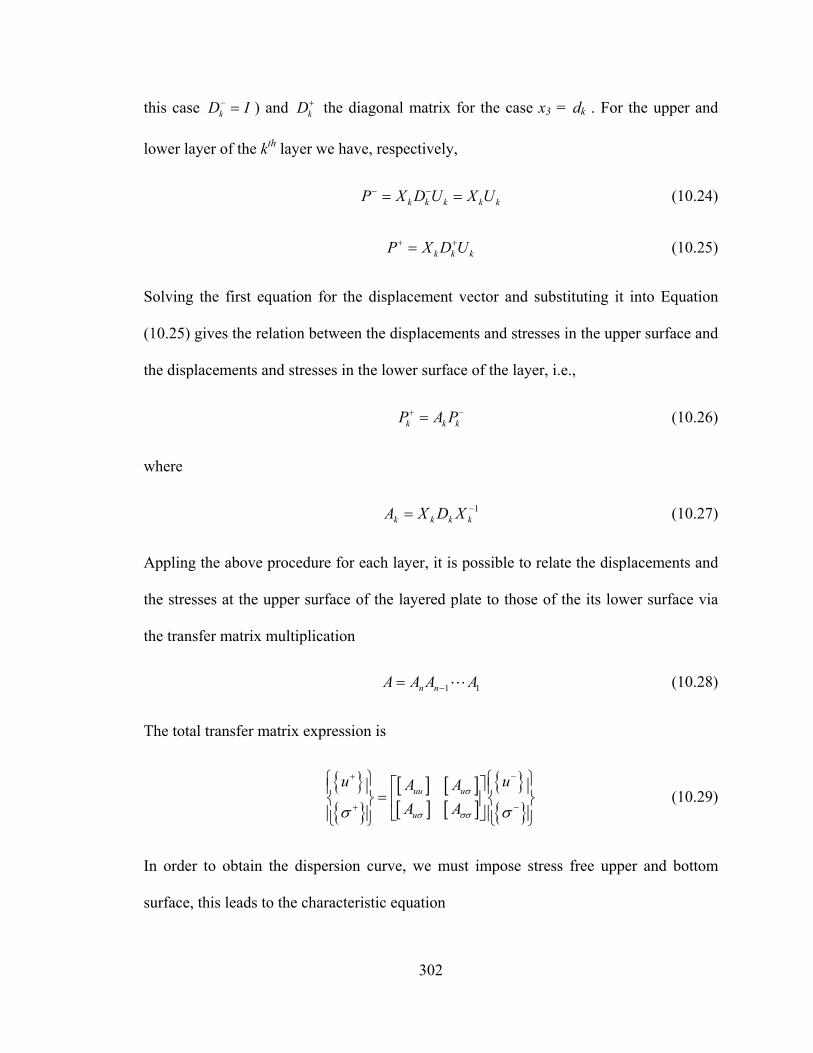
302
this case kD I− = ) and kD+ the diagonal matrix for the case x3 = dk . For the upper and
lower layer of the kth layer we have, respectively,
k k k k kP X D U X U− −= = (10.24)
k k kP X D U+ += (10.25)
Solving the first equation for the displacement vector and substituting it into Equation
(10.25) gives the relation between the displacements and stresses in the upper surface and
the displacements and stresses in the lower surface of the layer, i.e.,
k k kP A P+ −= (10.26)
where
1−= kkkk XDXA (10.27)
Appling the above procedure for each layer, it is possible to relate the displacements and
the stresses at the upper surface of the layered plate to those of the its lower surface via
the transfer matrix multiplication
1 1n nA A A A−= L (10.28)
The total transfer matrix expression is
{ }{ }
[ ] [ ][ ] [ ]
{ }{ }
uu u
u
u uA AA A
σ
σ σσσ σ
+ −
+ −
⎧ ⎫ ⎧ ⎫⎡ ⎤⎪ ⎪ ⎪ ⎪=⎨ ⎬ ⎨ ⎬⎢ ⎥⎣ ⎦⎪ ⎪ ⎪ ⎪⎩ ⎭ ⎩ ⎭
(10.29)
In order to obtain the dispersion curve, we must impose stress free upper and bottom
surface, this leads to the characteristic equation

303
0uA σ = (10.30)
In general, matrix uA σ is a complex matrix. Equation (10.30) means that the absolute
value of the determinant must be equal to zero. The determinant of uA σ is an implicit
relation between the wave number ξ and the phase velocity v. Equation (10.30) is quite
complicated and it is not possible to solve analytically in an explicit form. Numerical root
searching tools have to be used to search for the phase velocity for a given wavenumber.
We developed a computer code that derives the dispersion curves. The inputs are the
vector of the orientations of the layers and the material properties of each layer. The code
computes the transfer matrix for each layer in the global coordinate system and the total
transfer matrix (10.28) for different value of velocity and frequency. Through root search,
the final value of the velocity is found.
10.1.2 Dispersion curves for isotropic layers
Consider the case of a layer of an isotropic material, hence 11 22 33c c c= = , 12 13 23c c c= = ,
66 55 44c c c= = , and 66 11 122c c c= − , Equation (10.10) becomes
( ) ( )( )( ) ( )
2 211 66 1 11 66 3
2 266 66 2
2 211 66 1 66 11 3
0
0
0
c c v U c c U
c c v U
c c U c c v U
α ρ α
α ρ
α α ρ
⎧ + − + − =⎪⎪
+ − =⎨⎪
− + + − =⎪⎩
(10.31)
Note that, the second equation in the system is decoupled from the other two and it can be
solved separately. A non trivial solution to system (10.31) is found if the determinant of
the characteristic equation is equal to zero, i.e., if
4 21 2 0A Aα α+ + = (10.32)

304
where
( ) ( ) ( )
( )( )
22 211 66 66 66 11 66
1
2 211 66
2
c c v c c v c cA
c v c vA
ρ ρ
ρ ρ
− + − − −=
Δ− −
=Δ
(10.33)
Recall that 66c μ= , 11 2c λ μ= + , 2 2pc λ μ
ρ+
= , and 2sc μ ρ= , solutions of Equation
(10.33) are
2
1 2 2
2 2
3 4 211
5 6 1
1
1 1
s
p
vc
v vc c
α α
ρα α
α α α
= − = −
= − = − = −
= − =
(10.34)
and the solution to system (10.31) is
333 3
13
355
15 5
1
UWUUWU
α
α
⎧ = =⎪⎪⎨⎪ = = −⎪⎩
(10.35)
The stress coefficients (10.21) simplify to
( )( )
( )
213 13 3 33 3 5
23 55 3 3 3
15 13 5 33 52
525 55 5 5
5
1
22
1
D c c W
D c WD c c W
D c W
α μ α
α μα
α μ
αα μα
= + = −
= + =
= + = −
−= + =
(10.36)
The expanded matrix form for the isotropic plate becomes (we do not consider the SH
wave)

305
( )
3 3
3 31
5 3
5 3
1 11
3 3 3 5 5 13*33 13 13 15 15 13*13 23 23 25 25 15
1 1 1 1 i x
i xi x vt
i x
i x
u U eu W W W W U e
eD D D D U eD D D D U e
ξα
ξαξ
ξα
ξα
σσ
−−
−
⎡ ⎤⎡ ⎤ ⎡ ⎤⎢ ⎥⎢ ⎥ ⎢ ⎥− − ⎢ ⎥⎢ ⎥ ⎢ ⎥=⎢ ⎥⎢ ⎥ ⎢ ⎥⎢ ⎥⎢ ⎥ ⎢ ⎥− − ⎢ ⎥⎣ ⎦ ⎣ ⎦ ⎣ ⎦
(10.37)
Figure 10.4 shows that the dispersion curves derived through transfer matrix method are
exactly the same as those derived through solution of the Rayleigh – Lamb equation.
Same results are obtained either we consider a single layer aluminum plate of 1-mm
thickness or a two-layer aluminum plate of total thickness 1 mm. The derivation for
isotropic layer is useful if we want to study joints of metal layers.
Figure 10.4 Comparison of dispersion curves predicted by layered model (transfer matrix
method) vs. isotropic classic theory (Rayleigh – Lamb equation). a) One-layer
aluminum plate 2024-T3, 1-mm thick. b) Two-layer aluminum plate 2024-T3, 1-mm
total thickness. Dash lines: values derived from the Rayleigh – Lamb equation; Solid
lines: values derived from the transfer matrix method.
10.1.3 Dispersion curves for unidirectional composite plates
Let consider a plate made of one layer of unidirectional fibers. If we consider the wave
propagation in the direction of the fiber (θ = 0°) or perpendicular to the fiber (θ = 90°)
0 1000 2000 3000
2000
4000
6000
Phas
e ve
loci
ty (m
/s)
f (kHz) 0 1000 2000 3000
2000
4000
6000
f (kHz)
Phas
e ve
loci
ty (m
/s)
One-layer Two-layer

306
the shear horizontal wave is decoupled from the other two modes and they can be derived
separately (see Equation (10.11).) The code developed can compute the dispersion curves
for plate made of one unidirectional layer. We tested our computer code results versus
results found in Nayfeh (1995) for graphite-epoxy plate θ=0 and θ=45. The values
derived with the code where the same as shows in the book.
Figure 10.5 shows the dispersion curves derived for a unidirectional composite plate
made of one layer of 65% graphite 35% epoxy for different wave propagation direction.
Figure 10.5 Dispersion curves for plate made of one unidirectional layer of 65% graphite 35%
epoxy (material properties from Nayfeh 1995) as derived by our code. a) θ = 0°; b) θ
= 18°; c) θ = 36°; d) θ = 90°.
0 1 2 3 4 5 6 7 80
1000
2000
3000
4000
5000
6000
0 1 2 3 4 5 6 7 80
1000
2000
3000
4000
5000
6000
0 1 2 3 4 5 6 7 80
1000
2000
3000
4000
5000
6000
ξd ξd
ξd ξd
cs
cs
a) b)
c) d)

307
For the case of wave propagating along the fiber direction or transversely to the fiber
direction, the quasi-SH wave is decoupled from the other two waves and it is possible to
derive the quasi-antisymmetric and quasi symmetric mode separately. The value of the
phase velocity of the quasi S0 mode at low frequencies decreases as the wave
propagation angle increases. The quasi SH0 wave phase velocity is not constant trough
the frequency range for wave propagation angle close to 45 degrees.
As mentioned the transfer matrix method is not stable for high frequency-thickness
products, in this case we obtain a plot similar to Figure 10.6.
Figure 10.6 Transfer matrix instability for high frequency-thickness products.
10.1.4 Group velocity in composite plates
Figure 10.7 shows the dispersion curves of the first quasi antisymmetric wave mode (A0)
propagating in a composite plate made of graphite epoxy. The dispersion curves shown
are for different angles of propagation (θ ) with respect to the fiber direction.
ξd
c (m
m/s
ec)

308
Figure 10.7 Dispersion curves for first antisymmetric wave mode (A0) propagating at different
angles with respect to the fiber direction. Plate material: 65% graphite 35% epoxy
(material properties from Nayfeh 1995).
The phase velocity is higher when the wave propagates along the fiber direction. As
the angle of the wave propagation direction increases, the phase velocity decreases till
reaching a minimum in the direction perpendicular to the fiber. This is due to the fact that
along the fiber the material stiffness is greater than all the other directions and it
decreases while θ increases.
Assume we are interest in finding the group velocity of the wave propagating along
direction θ with respect to the fiber direction. From literature (Rose 1999) we know that
the group velocity vector is perpendicular to the phase slowness curve. The phase
slowness is the inverse of the phase velocity; hence, the phase slowness curve shows the
dependence of the relative arrival time of a plane wave on the direction of wave
propagation.
c (m
/s)
fd
θ = 90°
θ = 54° θ = 36°
θ = 18°θ = 0°
θ

309
From the slowness curve (Figure 10.8), we find for the point of interest P the
perpendicular Ec at the slowness curve point P. The angle of the perpendicular to the
slowness curve at point P is equal to ψ . Hence, the group velocity magnitude is given by
cosE
ccφ
= (10.38)
where φ ψ θ= − . Knowing the magnitude of Ec and the angle ψ for each point on the
slowness curve, it is possible to construct the wave surface.
Figure 10.8 Slowness curve and notation
Figure 10.9 shows the slowness curve for the 65% graphite 35% epoxy unidirectional
plate. The slowness curve is derived from the inverse of the phase velocity of the wave
for any angle of propagation at a given frequency thickness product. The slowness curve
is different for each frequency thickness product.
Figure 10.10 shows the wave surface for the 65% graphite 35% epoxy unidirectional
plate at frequency thickness product of 400 kHz-mm (solid line) and 1700 kHz-mm (dash
line) derived through Equation (10.38).
Ec
φ
θ ψ
1 ccP

310
Figure 10.9 Slowness curve for unidirectional 65% graphite 35% epoxy plate. Solid line:
frequency thickness product of 400 kHz-mm; Dash line: frequency thickness product
of 1700 kHz-mm. Values are 41 10c ⋅ .
Figure 10.10 Wave front surface for unidirectional 65% graphite 35% epoxy plate. Solid blue line:
frequency thickness product of 400 kHz-mm; Dash red line: frequency thickness
product of 1700 kHz-mm.
As shown in Figure 10.10, the wave surface is quite different from that of the slowness
surface. Hence, there is difference between the phase velocity propagation directions and
Fiber directionψ
Fiber direction θ
1c

311
amplitude and the group velocity propagation directions and amplitude. This phenomena
is quite important for directional transducers such as wedge transducers, comb
transducers, or rectangular PWAS transducers
10.1.5 Dispersion curves for quasi-isotropic composite plates
Experimental values and theoretical predictions of dispersion curves have been derived
for a quasi-isotropic plate [(0/45/90/-45)2s] Uni Tape T300/5208 with 2.25-mm thickness
and 1240×1240-mm size. The material properties are reported in Table 10.1.
Table 10.1 Ply material properties (Herakovich 1998)
T300/5208
Density (g/cm3) 1.54
Axial Modulus E1 (GPa) 132
Transverse Modulus E2 (GPa) 10.8
Poisson’s ratio ν12 0.24
Poisson’s ratio ν23 0.59
Shear Modulus G12 (GPa) 5.65
Shear Modulus G23 (GPa) 3.38
Modulus ratio E1/E2 12.3
Axial tensile strength XT (MPa) 1513
Transverse tensile strength YT (MPa) 43.4
Strength ratio XT/YT 35
The dispersion curves obtained from the code developed in our laboratory are
represented in Figure 10.11. From the output values of the program it is possible to
extract the first 3 modes of interest and convert the plot from wavenumber-thickness to
frequency-thickness representation. From the phase velocity it is possible to calculate the
group velocity curves as shown in Section 10.1.4.

312
Figure 10.11 Dispersion curves for a quasi-isotropic plate [(0/45/90/-45)2s]. (a) output from the
program; (b) elaboration of S0, SH, A0 modes.
Due to the properties of the quasi-isotropic materials, we expect that the phase
velocity magnitude to be almost constant for any propagation angle. The theoretical
values of the phase velocities are plotted in Figure 10.12.
Figure 10.12 Phase velocities for a quasi isotropic plate. Theoretical values for 0θ = ° , 90θ = ° ,
45θ = ° , and 135θ = °
S0
A0
SH
S0
A0
SH
ξd
(a)
(b)
0
1000
2000
3000
4000
5000
6000
0 100 200 300 400 500 600 700f (kHz-mm)
c (m
/s)
quasi S0
quasi SH0
quasi A0
0θ = °90θ = °
45θ = °135θ = °
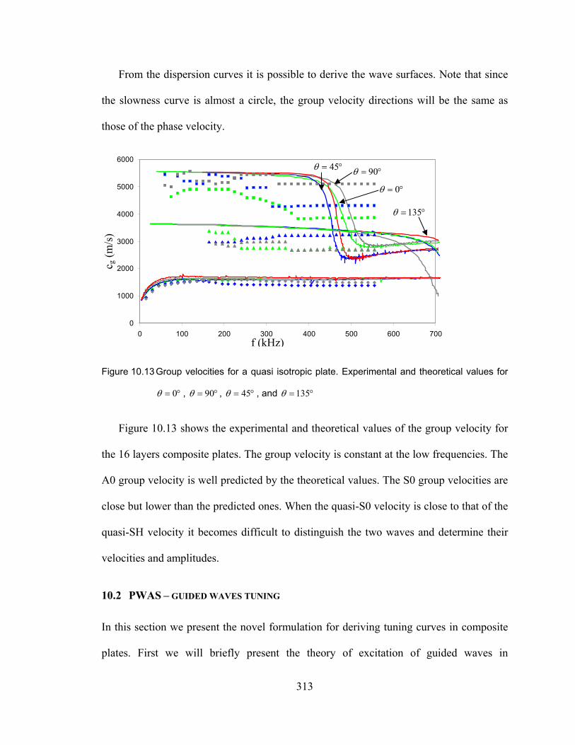
313
From the dispersion curves it is possible to derive the wave surfaces. Note that since
the slowness curve is almost a circle, the group velocity directions will be the same as
those of the phase velocity.
Figure 10.13 Group velocities for a quasi isotropic plate. Experimental and theoretical values for
0θ = ° , 90θ = ° , 45θ = ° , and 135θ = °
Figure 10.13 shows the experimental and theoretical values of the group velocity for
the 16 layers composite plates. The group velocity is constant at the low frequencies. The
A0 group velocity is well predicted by the theoretical values. The S0 group velocities are
close but lower than the predicted ones. When the quasi-S0 velocity is close to that of the
quasi-SH velocity it becomes difficult to distinguish the two waves and determine their
velocities and amplitudes.
10.2 PWAS – GUIDED WAVES TUNING
In this section we present the novel formulation for deriving tuning curves in composite
plates. First we will briefly present the theory of excitation of guided waves in
0
1000
2000
3000
4000
5000
6000
0 100 200 300 400 500 600 700f (kHz)
c g (m
/s)
0θ = °
90θ = °45θ = °
135θ = °

314
composites plates as derived by Xi (2002) and we will show its limitations. Then, we will
extend the NME method to the case of composite plates.
A series of experiments where performed to determine the behavior of the tuning
between PWAS and structure in composite materials. A preliminary theoretical
development of tuning on composite has been developed and comparison with
experiments has been performed.
10.2.1 Excitation of guided waves
To derive PWAS tuning on isotropic plate it is possible to derive through Fourier
transformation method a close form solution as shown in Giurgiutiu (2008) and in
Section 7 of this dissertation. Xi (2002) extended the integral transform solution derived
for isotropic plates to the case of composite plates.
The analytical solution of the inverse transform of the Fourier integral is in this case
to be solved numerically. The integral transform solution follow the global matrix
procedure; first the displacement solutions are transformed in the wavenumber domain
(Fourier transform) and then the global system equation for the entire laminate is
determined as AC T= % , where A is the global matrix for the composite plate, C consists
of constant vectors for the layers to be determined from the boundary conditions on the
upper and lower surfaces of the plate, and T% is the Fourier transform of the external
force. Vector C is obtained from the solution of AC T= % . Knowing the vector of
constants, it is possible to determine the displacement functions in the wavenumber
domain for all the layers in the laminate. To obtain the displacement in the space domain,
the following inverse Fourier transform integration must be solved.

315
1( , ) ( , )2
ikxU z x U z k e dkπ
∞ −
−∞= ∫ % (10.39)
Solution of equation (10.39) can be done numerically because analytical solution is not
possible. Moreover, even if a numerical method is used, a proper treatment is needed, as
the integrand goes to infinity at the poles on the integral axis.
A different method, NME, can be used to determine the transducer frequencies for
any kind of plates. Hereunder we will apply the NME developed in Sections 7 and 0 to
the case of composite plates. First we will recall some basic concept of the NME theory.
Figure 10.14 Plate subject to surface tractions
10.2.1.1 Power flow
One of the parameter that appears in the tuning through normal mode expansion is the
power flow of the wave mode under consideration in the direction of propagation of the
wave, i.e., x. Hereunder, we reassume the derivation of the power flow through the proof
of orthogonality of the guided wave modes. The proof of orthogonality requires one
general acoustic field theorems, i.e., the complex reciprocity relation. Recall the
expression of the complex reciprocity relation as expressed in Equation (5.37), i.e.,
( ) ( )1 2 2 1 1 2 1 2 1 2 2 1:t
ρ∂∇ ⋅ + ⋅ = ⋅ + − ⋅ − ⋅
∂v T v T v v T S v F v F%% %% % % (10.40)
2d
y
x
ty tx

316
where v1, T1 are field solutions driven by source F1, and v2, T2 are field solutions driven
by sources F2. The tilde sign above a quantity signifies complex conjugate, i.e., if
c a ib= + , then c a ib= −% .
Assume that the source terms are equal to zero, i.e. 1 2 0= =F F , and that all field
quantities varies as i te ω , therefore it
ω∂→
∂. It is apparent that the time dependent terms
i te ω and i te ω− in Equation (10.40) cancel out, and the first term on the right hand side
becomes
( ) ( )1 2 1 2 1 2 1 2: : 0i t i t i t i te e e et t
ω ω ω ωρ ρ− −∂ ∂⋅ + = ⋅ + =
∂ ∂v v T S v v T S% %% % (10.41)
With these assumptions, Equation (10.40) becomes
( )1 2 2 1 0∇ ⋅ + ⋅ =v T v T% % (10.42)
Assume that solutions “1” and “2” are free modes with propagating factors ξm and ξn
respectively, and hence they can be written as
1
2
( , )
( , )
m
n
i xm
i xn
e y z
e y z
ξ
ξ
−
−
=
=
v v
v v and 1
2
( , )
( , )
m
n
i xm
i xn
e y z
e y z
ξ
ξ
−
−
=
=
T T
T T (10.43)
The structure under consideration is a layered waveguide structures with arbitrary
anisotropy and inhomogeneity. We can assume that the properties do not vary along z
direction. In the case of anisotropy, this can be achieved by choosing as reference axis the
principal coordinate system, hence Equation (10.43) becomes
1
2
( )
( )
m
n
i xm
i xn
e y
e y
ξ
ξ
−
−
=
=
v v
v v and 1
2
( )
( )
m
n
i xm
i xn
e y
e y
ξ
ξ
−
−
=
=
T T
T T (10.44)

317
Substitute the field expressions in Equation (10.44) into the complex reciprocity relation
(10.42) and explicit the del operator to obtain after rearrangement
( )( ) ( ) ( ) ( )m n m ni x i xm n n m m n n m m ni e e
yξ ξ ξ ξδξ ξ
δ− − − −− − ⋅ − ⋅ ⋅ = − ⋅ − ⋅ ⋅v T v T x v T v T y
% %% % %% % (10.45)
Integrate with respect to y Equation (10.45) to get
( ) ( )4d
m n mn n m m n di Pξ ξ
−− = − ⋅ − ⋅ ⋅v T v T y% %% (10.46)
where Pmn is power flow defined as
( )1 Re4
d
mn n m m nd
P dy−
= − ⋅ − ⋅ ⋅∫ v T v T x%% (10.47)
Assume either stress-free or rigid acoustic boundary conditions, i.e. 0⋅ =T y or 0=v at
y d= ± ; the right-hand side of Equation (10.46) is zero. Equation (10.46) becomes
( )4 0m n mni Pξ ξ− =% . (10.48)
This is the expression of the orthogonality relation for the waveguide modes. Equation
(10.48) is satisfied for
i. m nξ ξ= % if 0mnP ≠ ;
ii. 0mnP = if m nξ ξ≠ % .
The frequency spectrum shows that the waves modes occur in pairs with equal and
opposite wavenumber ξ. For propagating modes ξm is real, then Equation (10.47) can be
written as

318
( )2
2
1Re2
b
nn n nb
P dy−
= − ⋅ ⋅∫ v T x% (10.49)
nnP is nonzero and represents the average power flow of the nth mode in the x direction
per unit waveguide width (in the z direction) (see Figure 10.14).
10.2.1.2 Tuning of guided waves
For the study of excitation of waveguide modes, the starting point is the complex
reciprocity relation (10.40). In this case we retain terms F1 and F2. but we still assume
time harmonic waves. Relation (10.40) becomes
( ) ( )2 1 1 2 2 1 1 2 2 1 1 2y xδ δ
δ δ− ⋅ − ⋅ ⋅ + − ⋅ − ⋅ ⋅ = +v T v T y v T v T x v F v F% % %% % % (10.50)
Consider the case of a PWAS bonded on the top surface of a composite plate. In this
case, the wave guides can be excited at the acoustic boundaries by traction forces only,
⋅T y . We assume that the excited field (solution “1”) can be represented by mode
expansion as in Equation (7.8), i.e.,
1 1
1 1
( , ) ( ) ( )
( , ) ( ) ( )
n nn
n nn
x y a x y
x y a x y
= =
= =
∑
∑
v v v
T T T (10.51)
We assume also that solution “2” is of the type
2 2
2 2
( , ) ( )
( , ) ( )
n
n
i xn
i xn
x y y e
x y y e
ξ
ξ
−
−
= =
= =
v v v
T T T with 2 0=F (10.52)
Integrating Equation (10.50) with respect to y, we obtain
( ) ( )2 1 1 2 2 1 1 2 0d d
d d
dy dyy x
δ δδ δ− −
− ⋅ − ⋅ ⋅ + − ⋅ − ⋅ ⋅ =∫ ∫v T v T y v T v T x% %% % (10.53)

319
Substituting solutions (10.51) and (10.52) into Equation (10.53), we obtain
( )
( )
1 1
( ) 0
n
n
d i xn n d
di x
m n m m nm d
e
e a x dyx
ξ
ξδδ
−
−
− ⋅ − ⋅ ⋅
⎛ ⎞+ − − ⋅ =⎜ ⎟
⎝ ⎠⋅ ⋅∑ ∫
v T v T y
v T v T x
%
%
%%
%% (10.54)
Recall Equation (10.49), hence we get
( )1 1 ( ) 0n nd i x i x
n n m nmd m
e e a x Px
ξ ξδδ−
⎛ ⎞− ⋅ − ⋅ ⋅ + =⎜ ⎟⎝ ⎠
∑v T v T y % %%% (10.55)
According to the orthogonality relation (10.48), the summation in (10.55) has only one
nonzero term. Considering the propagating mode n (ξn real), Equation (10.55) can be
written as
( )4 ( )d
nn n n n n dP i a x
xδ ξδ −
⎛ ⎞+ = ⋅ + ⋅ ⋅⎜ ⎟⎝ ⎠
v T v T y%% (10.56)
where
( )1 1Re Re4 2
d d
nn n n n n n nd d
P dy dy− −
⎡ ⎤ ⎡ ⎤= − ⋅ − ⋅ ⋅ = − ⋅ ⋅⎢ ⎥ ⎢ ⎥
⎣ ⎦ ⎣ ⎦∫ ∫v T v T x v T x%% % (10.57)
Assume that the anisotropic plate is loaded over a finite portion in the y direction on the
upper surface by an infinite width traction force in the x direction
( ) ( ) ( )i t i ty xx e t x t x eω ω⎡ ⎤⋅ = = +⎣ ⎦T y t y x (10.58)
The right end side of Equation (10.56) becomes
( ) ( )( ) ( , ) ( , ) ( ) ( )d
n n ndy x y x y y d x
−⋅ ⋅ + ⋅ ⋅ = ⋅v T y v T y v t%% % (10.59)

320
The second term on the left-hand side is zero because we assumed traction free boundary.
Finally Equation (10.56) becomes
( )4 ( ) ( )nn n n nP i a x d xx
δ ξδ
⎛ ⎞+ = ⋅⎜ ⎟⎝ ⎠
v t% (10.60)
This is a first-order ODE that governs the amplitudes of the general modes. Its solutions
is
( )( ) ( )4
nn
xi xix
n nnn c
ea x d e dP
ξη η η
−
= ⋅ ∫v t% (10.61)
Where c is a constant used to satisfy the boundary conditions. Let the external tractions t
to be nonzero only in the interval a x a− ≤ ≤ , we can write the solution as (see Section
7.1)
( )( ) ( ) for 4
n n
ai x i xn
nnn a
da x e e x dx x aP
ξ ξ−+
−
= ⋅ >∫v t% (forward wave solution) (10.62)
The strain, hence the tuning curves, on the top surface of the plate is given by
1( ) ( ) ( ) ( )i t i tx n x n n x
n na x v y e dt a x v y e
xω ωε ξ
ω∂
= =∂ ∑ ∑∫ (10.63)
or in expanded form using Equation (10.62)
( ) ( ) ( ) for 4
n n
ai x i xi tn
x x nnnn a
d v y e e e x dx x aP
ξ ξωε ξω
−
−
= >∑ ∫v t%
(10.64)
This represents the tuning expression of the strain in the composite plate excited by the
PWAS. This derivation is formally equal to the case of an isotropic plate. The number of
modes present depends on the material properties of the composite plate. For the case of a

321
composite plate made of one layer of unidirectional fibers, the PWAS will excite only
Lamb modes (symmetric and antisymmetric) if we consider propagation along the fibers
or transverse to the fibers. In all other cases, three waves will be present.
The main difficult in solving Equation (10.64) lies in the derivation of the average
power flow. The average power flow is given by the integral over the plate thickness of
the velocity by the stress, and it must be performed numerically.
Recall the definition of the average power flow as given by Equation (10.57), i.e.,
( )1 ˆRe2
d
nn n ndP dy
−= − ⋅ ⋅∫ v T x% (10.65)
Consider the nth wave mode propagating in the kth layer of the composite plate (for
simplicity of notation we drop the subscript n), the integrand of Equation (10.65) is given
by
( ) 1 1 2 6 3 4ˆ v T v T v T⋅ ⋅ = + +v T x% % % % (10.66)
where the velocities are defined as
( ) ( ) ( )1 36
1 2 3 11
, , 1, , qi x x vtq q q
qv v v i v V W U e ξ αξ + −
=
= − ∑ (10.67)
and the stresses are defined as
( ) ( )1 3
1 11 13 16
4 44 45 1
6 16 36 66
q
q q qi x x vt
q q q q qq
q q q
T c c W c VT i c V c W U eT c c W c V
ξ αα
ξ α α
α
+ −
+ +⎧ ⎫ ⎧ ⎫⎪ ⎪ ⎪ ⎪= + +⎨ ⎬ ⎨ ⎬⎪ ⎪ ⎪ ⎪+ +⎩ ⎭ ⎩ ⎭
∑ (10.68)
Once the dispersion curves are known, the stress and the velocity in each layer for each
mode are known and, hence, the average power flow can be computed. It is to be

322
emphasized that the derivation of the tuning curves presented here does not depend on the
particular method used to derive the dispersion curves.
The integral in Equation (10.64) depends on the assumption made on the bond layer
between PWAS and structure. For the composite plate, we assume that the thickness of
the bond layer approaching zero, i.e. we assume ideal bond conditions.
In the case of ideal bonding solution, the shear stress in the bonding layer is
concentrated at the ends of the PWAS tips. We can use the pin-force model to represent
the load transferred form the PWAS to the structure, i.e.,
( ) ( )0 if
( , )0 if
a x a x a x ax d
x a
τ δ δ⎧ − − + ≤⎡ ⎤⎪ ⎣ ⎦= ⎨>⎪⎩
xt (10.69)
Substituting (10.69) into Equation (10.64), we obtain:
( ) ( )0
00
( ) ( )4
n n n
ai x i x i xi tn
x x nnnn a
da v y e e x a e dx x a e dxP
ξ β ξωε τ ξ δ δω
− −
−
⎡ ⎤= − − +⎢ ⎥
⎣ ⎦∑ ∫ ∫
v% (10.70)
where, the term 0aτ is a constant depending on the excitation, the term ( ) 4nx nnv d P% is the
excitability function of mode n (depends on the mode excited and not on the source used
for excitation), and the term in square brackets is the Fourier integral of the excitation.
The integral solution is
( ) ( )0
0
2 sinn n
ai x i x
na
x a e dx x a e dx i aβ ξδ δ ξ−
−
− − + = ±∫ ∫ (10.71)
Substituting this result into Equation (10.64), we obtain:
( ) ( ) sin2
ni xi tnx x n n
nnn
di v y e e aP
ξωε ξ ξω
−= ∑v% (10.72)

323
10.2.2 Experimental results and theoretical predictions
A set of experiments where performed to verify the presence of the tuning between
PWAS and an anisotropic host structure. Pitch-catch experiments were performed in
which one PWAS served as transmitter and another PWAS served as receiver. The signal
used in the experiments was a Hanning-windowed tone burst with 3 counts. The signal
was generated with a function generator (Hewlett Packard 33120A) and sent through an
amplifier (Krohn-Hite model 7602) to the transmitter PWAS. A data acquisition
instrument (Tektronix TDS5034B) was used to measure the signal measured by the
receiver PWAS. The plate used in the experiments was a quasi-isotropic composite plate
[(0/45/90/-45)2]S, of T300/5208 Uni Tape with 2.25-mm thickness and size 1240×1240-
mm (material properties are reported in Table 10.1). Figure 10.15 shows the layout of the
experiments, the figure represents the central part of the composite plate.
Figure 10.15 Experiment layout for [(0/45/90/-45)2]S, of T300/5208 Uni Tape with 2.25-mm
thickness and size 1240x1240-mm.
0º
90º
T
S2
R1
S1
R3
R2
R4 R5
S3

324
The PWAS denoted with the letter T was the transmitter while the others were
receivers. The distance between the receivers and the transmitter was 250 mm. The angle
between the receivers was 22.5º. The frequency of the signal was swept from 15 to 600
kHz in steps of 15 kHz. At each frequency, we collected the wave amplitude and the time
of flight for the waves present in the plate. A problem, faced in the experiments, was the
efficacy of the ground. To obtain a strong signal the ground was provided by bonding a
sheet of copper on the composite surface. In this way the signal was strong and consistent
during the experiments.
10.2.2.1 Round PWAS
Experiments with round PWAS diameter 7-mm, 0.2-mm thick (American Piezo Ceramics
APC-850) were performed with the layout shown in Figure 10.15. Three waves were
detected: quasi-S0, quasi-A0, and quasi-SH0.
Figure 10.16 Tuning Experimental data for a round PWAS for different propagation directions. a)
quasi-A0 mode; b) Quasi-S0 mode and quasi-SH0 mode
Figure 10.16 shows the waves amplitudes as detected by PWAS R1, R2, R3, R4, and
R5, corresponding to the directions 0º, 22.5 º, 45º, 67.5 º, and 90º. The quasi-A0 mode
0
2
4
6
8
10
12
14
16
18
0 100 200 300 400 500 6000
2
4
6
8
10
12
14
16
18
0 100 200 300 400 500 600
f (kHz) f (kHz)
V (m
V)
a) b)
0°
22°
45° 67°
90°
0° 22°
45°
67°
90°

325
reached its maximum before the quasi S0 mode maximum. The quasi SH wave had
amplitude one forth of the S0 mode.
10.2.2.2 Square PWAS
The layout of the experiment is shown in Figure 10.15, transducer S1 was used as
transmitter while transducer S2 was used as receiver. Figure 10.17a shows the
experimental amplitudes of the three waves. The A0 mode extinguishes as soon as the
quasi-SH wave appears. The wasi-S0 mode has a maximum at 450 kHz and then
decreases. The quasi-A0 and quasi-S0 modes have a slope similar to that of a metallic
plate.
Figure 10.17 Experimental and theoretical tuning values. a) Experimental data for square PWAS.
Triangles: quasi-A0 mode; Circles: quasi-S0 mode; Squares: quasi-SH0 mode. b)
Experimental vs. theoretical values for first antisymmetric mode.
Figure 10.17b shows the comparison between experimental and theoretical values for
quasi-antisymmetric mode. The theoretical curve follows the behavior of the
experimental one. Tuning curves through NME method seems to be a promising tool to
predict the interaction between PWAS and structure.
0
1
2
3
4
5
6
7
8
9
10
11
12
0 100 200 300 400 500 600 700f (kHz)
V (m
V)
A0 S0
SH
f (kHz) 0 100 200 300
5
10
a) b)

326
PART III STRUCTURAL HEALTH MONITORING ISSUES AND
APPLICATIONS

327
In Part III we discuss issues and applications of SHM.
First we address the problem of reliability of structural health monitoring methods.
SHM technologies have been studied in research laboratories and it has been used in
some applications. In order for SHM methods to be used extensively in application fields,
the quality of SHM inspections must be ensured. Non destructive evaluation (NDE)
inspections quality has been ensured through specification requirements that control the
inspection process and results. However, so far, SHM methods have been left without
precise guidelines and the best practice has been to follow the specification provided for
NDE. One of the NDE quality control tools is the probability of detection curves (POD).
We show the procedure to develop POD curves for SHM through permanent attached
PWAS on composite panels.
In this Part, we show that the SHM inspection method using PWAS is not only
capable of detecting damage but also to function in any environment. In particular, our
research focuses on the applicability of SHM using PWAS for space applications. We
present the experiments we performed to determine the PWAS damage detection ability
under extreme environment conditions.
A set of experiments was performed to asses the survivability and durability of SHM
systems for real space applications. The set of experiments were determined from the
space mission guidelines for the determination of space-qualified NDE techniques. The
results show that SHM through PWAS is able to be a space-qualified SHM method.

328
In NDE methods, the bond layer between transducer and structure is not taken into
consideration because NDE sensors are not permanently attached to the structure. In
SHM using PWAS, the sensors are permanently attached to the structure and hence it is
important to be aware of the quality of the bond layer before and during the SHM
process. Here, we present a set of experiments developed to determine the effect of
partial bonding of the PWAS to the structure using capacitance measurements. From the
analysis of the results, we conclude that capacitance measurements can be an effectively
integrated in SHM methods to check whether a detection of damage is due to a real
damage or a change in the transducer bonding quality (true call or false call). We
determine confidence intervals that can be used as reference values to determine the
status of the bonding between transducer and structure.
In Part III, we also address the problem of SH waves and Lamb was scattering from
damage. In particular we show the solution for the case of a non-through the thickness
crack in a plate when a SH wave is incident. For the more difficult case of Lamb waves
scattering from discontinuities, we present the formulation of the problem, but no
solution is provided.
In most of our experiments, the PWAS have been used as active sensor. In this case,
the PWAS interrogates the structure on demand with an excitation frequency determined
by the user. PWAS transducers can be also used as passive sensors. Since a crack
propagating in a structure or an object impacting a structure releases a sudden strain
energy in the structure, the propagating strain wave can be detected by PWAS
transducers placed in the structure. We present two theoretical models to predict the wave
propagation when such events occur in a structure.

329
11 RELIABILITY OF STRUCTURAL HEALTH MONITORING
Lately SHM methods have received increase attention and many significant
improvements have been made by the scientific community in terms of capability to
detect, locate, and determine the size of damage in structures. SHM technologies are
slowly transitioning from the research labs to the application fields in civil, naval,
nuclear, aeronautical, and aerospace engineering. Although SHM methods are a mature
technique, still they lack of specification requirements to control the inspection process
and the quality of the inspection results.
Hereunder we highlight the state of the art of the specification for SHM methods and
we discuss the differences between NDE and SHM inspection requirements. We show
how a first set of specification for SHM could be derived and in particular how POD
curves for SHM with permanent PWAS can be derived.
11.1 SPECIFICATIONS FOR QUALITY STRUCTURAL HEALTH MONITORING INSPECTION
In most of the engineering fields, and especially in the aerospace and aeronautical fields,
the design philosophy is based on the damage tolerant design approach. This approach
ensures safe operation in the presence of flows (Gallagher et al. 1984). In the 70’s the
reliability procedures for non-destructive inspection (NDI) was based on the principle
that the structural component as-manufactured is considered to have a flaw of length a0.
The length of the flaw is determined by the inspection capability of the manufacturing
process. The flaw length will increase during the component service till a critical size

330
after a determined time t0 of service. An inspection through noninvasive methods is
expected to be performed after a time equal to half t0. The inspection should be able to
detect flaws of a length aNDE, where length aNDE is based on the knowledge of the
probability of detection curves for that particular NDE method used (ASM Handbook
Vol.17). Figure 11.1 shows a typical POD for increasing length damage. As the damage
size increases, the probability (hence the ability) that the NDE method will detect the
damage increases. In an ideal condition, we would like the curve to step to high
probability rates quickly and at small damage lengths.
Figure 11.1 Typical probability of detection (POD) curves for increasing damage. (Grills, 2001)
So far, no standards have been defined for SHM inspections; in the absence of a
precise guide lines, the general approach to determine the reliability of SHM methods is
to rely on the standards derived for NDE methods. However, SHM methods are quite
different from NDE methods and hence the inspection guidelines used so far are not a
good assessment of SHM capabilities. The lack of a standard in SHM is one of the
motives that make difficult the transition from pure research to application.

331
The main difference between NDE and SHM is that SHM can be performed on the
component while on service and no shut down is required, hence, theoretically, the
component could be inspected continuously. However, since a great quantity of data is
collected every time a scan of the structure is performed, in reality, the SHM can not run
continuously. To determine the time interval between two inspections, we must know the
probability of detecting the critical flaw size. For this motive POD curves for SHM
methods are still needed for field applications. Since SHM is performed while the
structure is on service, the POD curves are not only structure specific but also affected by
thermal and mechanical loads.
The performance of NDE methods is influenced mostly by the human factor, i.e., the
operator that performs the NDI. On the other side, SHM is influenced by both the method
used to install permanently the sensors and the transducers location on the structure.
These two aspects would lead to the desire to have POD curves for each SHM
manufacture (those who install the transducers on the structure) and for each structure
components with SHM transducer on it.
In NDE techniques the geometry of the structure under inspection does not influence
the outcome of the inspection; on the contrary, SHM is mostly geometry driven, meaning
that each structure geometry needs its particular SHM configuration.
Since the transducers are permanently attached to the structures, the sensors and the
bonding layer undergo degradation due to aging, corrosion, temperature cycling, and
vibrations. Reliability test on PWAS have been performed in order to asses the capability
of the transducer to survive different environments (Lin et al. 2009). However, a
systematic design of experiment to asses the reliability of the SHM structure (transducer-

332
bond-structure component) during service is still needed. The SHM system as well
should be under routine schedule accordingly with the survivability and reliability results.
A last aspect that should be proved is the algorithms robustness of the software used
for damage detection.
Table 11.1 shows the basic steps needed to make SHM method with permanent
attached transducers a reliable system for health monitoring inspection. (Chambers et al.
2006, Kessler S. 2005)
Table 11.1 Health monitoring reliability needs.
Factor under test Experiments result SHM
guideline output
Geometry beam, plate, joints, welds, rivet hole, elbows, etc
Material metallic, composite (unidirectional, layup, etc)
SHM method
Phase-array, sparse array, pitch-catch, pulse-echo,
electro mechanical impedance
SHM algorithm
Minimum flaw size
Inspection interval for structure
Transducer-bond-wiring system Aging, corrosion
SHM system – structural
component Load, vibrations, fatigue
Survivability
Sensor installation method
Reliability
Inspection interval for
SHM system
A POD curve should be determined for each given configuration of SHM method,
structure, and SHM algorithm. In this way the minimum detectable flaw size for each

333
particular configuration can be determined. Survivability and reliability tests will give the
maximum safe life span for the SHM method, or the durability of the system.
11.2 PROBABILITY OF DETECTION CURVES
To determine the POD curves for a well established NDE method, several specimens
with different flaw sizes are needed. Often the term POD is used just to refer to a limit set
of experiment where a specimen (either with one flaw or multiple flaws) for each
different geometry of interest is used to determine whether the SHM system is able or not
(one hit-miss data) to detect damage.
In a more comprehensive design of experiment aimed to derive a single POD curve,
we will need N identical specimens with different flaw sizes in the same location with
identical SHM system configuration. If we are also interested in other geometry
characteristics of the flaw (such as depth or delamination location) another set of
experiments is needed.
Consider, as an example, we want to determine a suit of experiments for determining
the probability of detection (POD) of damage in composite specimens using SHM
methodology.
We specify that the SHM methodology for damage detection under study relies on
permanently-attached unobtrusive minimally invasive transducers that are left in place on
the structure and are interrogated at will. In particular, these experiments will use
piezoelectric wafer active sensors. Other SHM transducers may be used as long as they
meet the description "permanently-attached unobtrusive minimally invasive that are left
in place on the structure and are interrogated at will".

334
We set that the damage detection methodology will rely on the following techniques
that can be used with a single PWAS transducers installation:
• pitch-catch
• pulse-echo
• phased array
• electromechanical (E/M) impedance
The data analysis will rely on algorithms that can identify the presence of damage, locate
the damage, and characterize it.
First we need to determine the SHM set up used in the experiments. In this case,
PWAS transducers will be used as transmitters and/or receivers. The setup will be:
• Eight (8) individual PWAS forming a sparse network (7-mm diameter, 0.2-mm
thick)
• Four (4) rectangular PWAS arrays (50-mm by 5 mm)
The transducers installation is shown in Figure 11.2.
Figure 11.2 Transducer lay out and specimen dimensions (all dimension in mm).
700
500
150
200
100
150

335
In the next step we select the specimens. In this case we want to derive a first basic
knowledge of the SHM system capabilities on damage detection on composites. We
select:
• Specimen material: conventional carbon/graphite fiber epoxy matrix prepeg, each
ply 0.127-mm.
• Specimen dimensions: 500x700-mm
• Extra length is left in the vertical direction for mounting in tensile testing
machine. Adhesively bonded wedge-in attached to the ends
• Four different composite plates:
1. Unidirectional (04)s, eight plies (thickness ~1mm)
2. Cross-ply (02/902)s, eight plies (thickness ~1mm)
3. Balanced #1: (0/45/-45/90)s, eight plies (thickness ~1mm)
4. Quasi-isotropic: (0/45/90/-45)s, eight plies (thickness ~1mm)
In the third step, we determine the damage type and location. The damage will be a
seeded damage consisting of 20-mm round Teflon inserts. The damage will be placed in
the specimens as shown in Figure 11.3. Five positions are considered, as indicated. The
seeded damage will be used to produce initial damage and to make it propagate through
the application of load.

336
Figure 11.3 Seeded flaw location (A, B, C, D, E) in the composite specimens
The seeded damage will be placed in two thickness positions: symmetric, i.e. at t/2
where t is the specimen thickness; asymmetric, i.e., at t/5 from the top.
Last step is the most important; we select the number n of specimens needed to
achieve statistical significance. For each configuration, it is possible to derive a POD
curve (ASM Handbook Vol.17). The SHM method is applied to a number of tests articles
with different flaws. The POD curves are generated from the results of the campaign of
tests. To generate the POD curves and the CI of the resulting curve, we need to perform
the same test on several specimens.
Table 11.2 Summary of the specimen configurations (Note: A, B, C, D, E: seed location)
Unidirectional Cross-ply Balanced Quasi-isotropic
Flaw depth (0)s (0/90)s (45/0/-45)s (0/45/90/-45)s
t/2 n·ABCDE n·ABCDE n·ABCDE n·ABCDE
t/5 n·ABCDE n·ABCDE n·ABCDE n·ABCDE
To construct the POD curves, we must determine the probability to determine a defect
with the chosen SHM method for different damage size and the CI interval. Table 11.3
A: Centered B: Edge side C: Corner
E: Edge off-setD: Edge up
PWAS
Seeded fault

337
reports the 95% CI for different values of the probability (P) of detection and different
sample sizes (n). A graphical representation of these results is given in Figure 11.4a.
Table 11.3 95% CI amplitude for different sample sizes (n) and probabilities
Probabilities, P
0.10 0.25 0.5 0.75 0.90
10 0 0.3 0 0.5 0.2 0.8 0.5 1 0.7 1
20 0 0.2 0.1 0.4 0.3 0.7 0.6 0.9 0.8 1
30 0.03 0.2 0.13 0.4 0.37 0.63 0.6 0.87 0.8 0.97
40 0.03 0.17 0.15 0.38 0.38 0.62 0.62 0.85 0.82 0.97
50 0.04 0.18 0.16 0.36 0.38 0.62 0.64 0.84 0.82 0.96
60 0.03 0.17 0.17 0.35 0.4 0.6 0.65 0.83 0.83 0.97
70 0.04 0.16 0.17 0.34 0.4 0.6 0.66 0.83 0.84 0.96
80 0.05 0.16 0.17 0.33 0.41 0.59 0.68 0.82 0.84 0.95
90 0.06 0.16 0.18 0.32 0.41 0.59 0.68 0.82 0.84 0.94
n
100 0.05 0.15 0.18 0.32 0.42 0.58 0.68 0.82 0.85 0.95
For example, if the SHM method is able to detect a flaw with a probability of 0.90
(10 out of 100 are not detected), with a sample size of 20, there is a 95% of probability
that the observed probability of detecting a defect is between (0.8, 1). As we can see this
interval is quite large; things become worst as the probability of detection decreases (for
n=20 and p=0.5 the interval is from 0.3 to 0.7) (see Figure 11.4a).

338
Figure 11.4 Statistical criteria. a) 95% confidence interval of probability of detection for
increasing values of n. b) Acceptance criteria.
In order to obtain smaller CI we must choose high sample size. Once the desired
sample size is chosen, we must determine a criterion to determine whether the SHM
method detects or not the defect.
As an example, consider the case in which we are using pitch-catch method to
perform SHM on a specimen. The control variable it is the amplitude of the transmitted
wave. As the damage increases the amplitude is expected to decrease. The wave
amplitude is subject to oscillation due to the noise on the signal and other factors that are
not correlated with the damage. In order to determine the critical value of the wave
amplitude below which we can say that the difference is due to noise, we must create a
baseline of readings. Through the baseline readings it is possible to determine the signal
distribution and the percentile of the distribution. We are interested in high percentile
because, we will say that a reading does not belong to the baseline distribution if its value
is above a critical value that is the value of the 0.99 percentile (see Figure 11.4b).
0.0 0.2 0.4 0.6 0.8 1.0
0.0
0.2
0.4
0.6
0.8
1.0
lower and upper limit
prob
abili
ty o
f det
ectio
n
Sample size n, 95% CI1020304050
60708090100
Lower limit valuesas n increases
Upper limit valuesas n increases
0 5 10
0.0
0.1
0.2
0.3
0.4
0.5
Den
sity
0 5 10
0.0
0.1
0.2
0.3
0.4
0.5
Den
sity
Discrimination threshold
Noise orbaseline Signal
Criteria

339
To obtain the noise distribution or baseline, we must perform on each specimen N
data collection in the undamaged condition. Then the specimens are damaged and the
value of the amplitude is compared with the critical value.
A “bootstrap” technique is used to determine the critical value and the best number of
baseline to record.
As we can see from the example the number of specimen proposed is considerable
high. A thoroughly determination of POD curves for SHM methods is not only time
consuming but also expensive. However, we think that in the future more strict
requirements for the implementation of SHM on real application will require rigorous
POD derivations to make SHM as reliable and well accepted in the industrial community
as NDE technologies are now days.
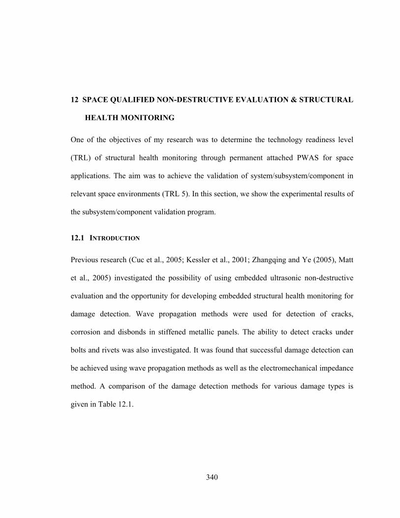
340
12 SPACE QUALIFIED NON-DESTRUCTIVE EVALUATION & STRUCTURAL
HEALTH MONITORING
One of the objectives of my research was to determine the technology readiness level
(TRL) of structural health monitoring through permanent attached PWAS for space
applications. The aim was to achieve the validation of system/subsystem/component in
relevant space environments (TRL 5). In this section, we show the experimental results of
the subsystem/component validation program.
12.1 INTRODUCTION
Previous research (Cuc et al., 2005; Kessler et al., 2001; Zhangqing and Ye (2005), Matt
et al., 2005) investigated the possibility of using embedded ultrasonic non-destructive
evaluation and the opportunity for developing embedded structural health monitoring for
damage detection. Wave propagation methods were used for detection of cracks,
corrosion and disbonds in stiffened metallic panels. The ability to detect cracks under
bolts and rivets was also investigated. It was found that successful damage detection can
be achieved using wave propagation methods as well as the electromechanical impedance
method. A comparison of the damage detection methods for various damage types is
given in Table 12.1.

341
Table 12.1 Summary of PWAS damage detection methods. (Cuc et al., 2005)
Wave Propagation Standing Wave Method Damage Pitch-Catch Pulse-echo Phased-Array EM Impedance
Disbond Fair Excellent -- Excellent Cracks -- -- Excellent Fair Corrosion -- -- -- Excellent Crack under bolt
Excellent Fair -- Fair
Delamination Excellent Excellent -- Excellent
As most of the space applications are moving towards composite material, a new set
of experiments was determined to validate the SHM system for space application on
composite structures. The space structural components are subjected to high loads and
extreme low temperatures, i.e., cryogenic temperature i.e., T=-300F (-185 C). We wanted
to prove: first, that the SHM system developed in our laboratory was able to perform
damage detection of different kinds on composite structures; second, that it was able to
withstand cryogenic temperatures (CT); and, third, that at the same time was able to
perform damage detection on composites at cryogenic temperatures.
12.2 SUBSYSTEM/COMPONENT SPECIFICATION
The basic element used for damage detection in these experiments was a round 7-mm
diameter, 0.2-mm thick PWAS. We proved that the piezoelectric material was able to
maintain actuation abilities in the cryogenic environments. To reproduce the cryogenic
temperature, we used containers immersed in liquid nitrogen since its liquid temperature
is approximately at the cryogenic temperature.
To check the ability to withstand CT and to operate in those conditions, a set of
experiments was performed in which a PWAS attached to a composite strip was
immerged ten times in a container with liquid nitrogen. Impedance data where taken

342
before each submersion. Figure 12.1a shows impedance signatures taken. It can be seen
that the material retained its peaks and their relative frequency location.
Figure 12.1b shows pitch-catch wave propagation before, during, and after
submersion of the specimen in liquid nitrogen. The data collected showed that the PWAS
was able to perform at cryogenic temperatures. It should be noted that the signal
propagated in the nitrogen had smaller peak to peak amplitude, but at the same time had
proportionately smaller background noise. The amplitude at room temperature (RT) after
submersion in liquid nitrogen did not return to original amplitudes. These experiments
were conducted with the transducers in direct contact with the liquid nitrogen. During
submersion some leakage of the wave in to the liquid can happen. In real application the
transducer will be not in contact with the liquid nitrogen.
Figure 12.1 Survivability and performance of PWAS under thermal fatigue. a) Indication of
survivability through resumption of resonant properties after submersion in liquid
nitrogen (PWAS, AE-15, room temperature). b) Wave propagation in composite for
various thermal environments. Comparison of a wave packet before, during, and
after submersion in liquid nitrogen.
0
500
1000
1500
2000
2500
3000
5 10 15 20 25 30 35 40Frequency (kHz)
Impe
danc
e (O
hms)
Baseline 1 Cycle2 Cyc les 3 Cycles4 Cyc les 5 Cycles6 Cyc les 7 Cycles8 Cyc les 9 Cycles10 Cycles
-25-20-15-10-505
10152025
0 50 100 150 200
Time (microseconds)
Ampl
itude
(mV
)
BaselineCryogenic1 Cycle
a) b)

343
The adhesive layer between the PWAS and the structure was a critical aspect.
Incorrect thickness, porosity, poor chemical preparation, etc. lead to poor transmission of
shear energy. The adhesive selected was Vishay M-Bond AE-15 (2-component) since it
was able to retain its properties even at the required temperatures. Su/Pb solder was used
for standard RT applications. Since at CT lead becomes brittle, indium was used in CT
applications because of the materials ability to retain mechanical properties even at CT.
In order to test the performance of the PWAS on various types of composite materials
and structures; four different test specimens were utilized. The first type of specimen was
a composite strip made of unidirectional fibers. The specimen was 400 x 51-mm (16”x2”)
and 1-mm thick. The fibers direction was parallel to the longest direction of the
specimen. A schematic of this specimen is shown in Figure 12.2. Two composite strips
were used with two PWAS installed on each at a distance of 150 mm. We used the
unidirectional strips to test damage detection of through holes at room temperature. In
one of the strip the hole was in line with two PWAS, in the second specimen the hole was
off-set from the pitch-catch path.
Figure 12.2 Unidirectional composite strips with PWAS installed. a.) Hole in the pitch-catch path;
b.) Hole off-set from the pitch-catch path.
Fiber direction
PWAS 0 PWAS 1
Pitch-catch path Damage
Fiber direction
PWAS 0 PWAS 1
a)
b)

344
The second type of specimen used was a quasi-isotropic composite plate [(0/45/90/-
45)2]S, of T300/5208 Uni Tape with 2.25-mm thickness and 1.200×1.200-mm size
(4’x4’). The composite panel specimen was used to investigate the PWAS damage
detection performance at room temperatures both for through-hole detection and impact
damage detection. A schematic of the test specimen and experimental setup used during
the experiments are shown in Figure 12.3.
Figure 12.3 Experimental setup for quasi-isotropic plate experiments. The damage sites are
marked as: (i) “Hole” for a through hole of increasing diameter; and (ii) I1, I2 for two
impacts of various energy levels.
The third type of specimen used during the experimental characterization of the
PWAS was a composite lap joint. For this specimen, material and layers lay-up was not
specified. The geometry of the specimen is shown in Figure 12.4. The specimen was built
with 16 seeded defects inside (Teflon patches), 8 on two rows distant respectively 76 mm
(3”) and 152 mm (6”) from the longitudinal edge. The thickness of the joint was about 13
mm (5/8”). The 8 patches in each row are approximately equidistant. We performed the
PWAS ComputerTektronix GPIB GPIB
8-pin ribbon
t
Parallel PortASCU2-PWAS
HP
33120
8-channel

345
following tests on this specimen: damage detection at room temperature with PWAS pair
1; damage detection at cryogenic temperature with PWAS pair 2; damage detection at
cryogenic temperature under uni-axial load with PWAS pair 3.
Figure 12.4 Lap joint; Teflon patches location (crosses) and PWAS location (circles).
The fourth type of specimen (Figure 12.5) utilized during the experimental testing
was a thick plate. As for the previous specimen, material and layers lay-up was not
specified. The composite tank interface specimen had plate of dimension 305 x 229-mm
(12”x9”) and thickness about 7 mm (1/4”). The specimen was fabricated with 16 patches
of different sizes located between various plies. Two experiments were performed on the
specimen: patch detection at room temperature; patch detection at cryogenic temperature.
Figure 12.5 Schematic of thick composite specimen and location of Teflon inserts (crosses).
P01 P00

346
Table 12.2 summarize the specimens used, the type of damages, the environmental
condition, and the methods used in the experiments. The data collected in each
experiment were analyzed using damage index (DI) software developed in our lab. The
DI software was used to assess the severity of the damage in each test run. The DI is a
scalar quantity that results from the comparative processing of the signal under
consideration. The damage metric should reveal the difference between readings
(impedance spectrum or wave packets) due to the presence of damage. Ideally, the DI
would be a metric, which captures only the spectral features that are directly modified by
the damage presence, while neglecting the variations due to normal operation conditions
(i.e., statistical difference within a population of specimens, and expected changes in
temperature, pressure, ambient vibrations, etc.). To date, several damage metrics have
been used to compare impedance spectra or wave packages and assess the presence of
damage. Among them, the most popular are the root mean square deviation (RMSD), the
power, the mean absolute percentage deviation (MAPD), and the correlation coefficient
deviation (CCD) (Giurgiutiu, 2008). In our experiments we have used the RMSD DI
shown in Equation (12.1).
( ) ( ){ }
( ){ }
20
20
Re Re
Re
i in
in
S SRMSD
S
−=
∑
∑ (12.1)
RMSD yields a scalar number, which represent the relationship between the compared
readings. The advantage of using this method is that the data do not need any
preprocessing, i.e., the data obtained from the measurement equipment can be directly
used to calculate the DI.

347
Table 12.2 Summary of experiments discussed in this paper.
Specimen Damage Environment Loading Methods
Unidirectional strips Hole RT Free P-C
Hole Composite panel
Impact damage RT Free P-C, P-E
RT Free Lap-joint Impact damage
CT Free P-C
RT Thick plate Delamination
CT Free P-C
12.3 DAMAGE DETECTION EXPERIMENTS ON TEST SPECIMENS
12.3.1 Unidirectional composite strips
The initial testing of the PWAS based damage detection began with unidirectional strips
shown in Figure 12.2. In both strips we installed two round PWAS 150 mm apart and we
used the pitch-catch method to detect the damage. In the first experiment, we determined
the smallest through-hole diameter that was detectable by the PWAS when the through-
hole was centered with the PWAS pair (see Figure 12.2a). In the second experiment, we
determined the smallest detectible hole diameter when the hole was offset 20 mm with
respect to the pitch-catch path (see Figure 12.2b).
Five baseline readings were taken when the strips were undamaged; then, a hole with
0.8-mm diameter was drilled on each specimen. The holes were enlarged in 11 steps until
they reached 6.4 mm in diameter. For each step, we took five pitch-catch readings. Table
12.3 reports the dimensions of the hole for each step and reading.

348
Table 12.3 Hole sizes for corresponding readings in the unidirectional composite strip
experiments.
Step # Readings Hole size (mm) Step # Readings Hole size (mm)
0 00 – 04 -- 6 31 – 35 3.2
1 05 – 09 0.8 7 36 – 40 3.6
2 10 – 14 1.5 8 41 – 45 4.0
3 15 – 19 1.6 9 46 – 50 4.8
4 20 – 25 2.0 10 51 – 55 5.5
5 26 – 30 2.4 11 56 – 60 6.4
On the unidirectional composite strips, the excitation signal used was a 3 count tone
burst at 480 kHz, which resulted in the strongest S0 wave packet. The signals were
analyzed using the RMSD DI and the results are shown in Figure 12.6 for both the
centered and off-center hole cases. Each dot in the graph represents a reading (there are 5
readings for each step to indicate reproducibility). The first 5 readings are the baseline
readings, i.e., the strip without damage.
Figure 12.6a shows that the DI increases monotonically with the increasing hole size
which will allow for easy interpretation of the DI in relation to the damage size.
0
0.05
0.1
0.15
0.2
0 5 10 15 20 25 30 35 40 45 50Reading #
DI v
alue
Figure 12.6 DI analysis of the damaged unidirectional composite strip. a.) Hole in the pitch-catch
path; b.) Hole off-set from the pitch-catch path.

349
Figure 12.6b shows that initially the DI value for off-axis hole increases
monotonically, but then the DI value plateaus at 1.5 mm and it jumps again when the hole
diameter reaches 3.2 mm. This indicates that, in unidirectional composites, off-axis
damage increase may be more difficult to detect and identify compared to centered
damage.
Since in every experiment conducted, the variance within each step is quite small,
from now on we will report only the mean value of the readings in each step.
12.3.2 Quasi-isotropic composite laminate
For the quasi-isotropic composite plate, two different kinds of damage, through-hole and
impact damage, were investigated at room temperature conditions. Twelve PWAS were
installed in a sparse array on the quasi-isotropic composite plate as shown in Figure 12.3;
the distance between the 6 PWAS pairs was 30 mm. In this case, the data was collected
automatically through ASCU2 system with an input voltage of the signal from the
function generator of 11 V (Figure 12.3). The 11-V limit was the maximum input voltage
that it is possible to send through ASCU2. The excitation signal used during the
interrogations was a 3 count tone burst at central frequency 54 kHz and 255 kHz. These
frequencies were selected through Lamb wave tuning experiments to maximize the A0,
and S0 wave modes. At 54 kHz, it was possible to obtain the maximum pseudo A0 mode;
at 255 kHz we obtained the maximum pseudo S0.
12.3.2.1 Detection of through-holes
In the through-hole detection case, data was collected from PWAS 0, 1, 5, 8, 12, and 13
(Figure 12.3). Each PWAS was in turn a transmitter and a receiver. Readings were taken
with the plate in an undamaged state and the plate in a damaged state. Four baseline

350
readings were taken in the undamaged configuration. A hole was drilled between PWAS
1 and 12. The location of the hole was halfway between these two PWAS. The diameter
of the hole was increased in 13 steps. At each step four readings were recorded. Table
12.4 reports for each step, the number of readings recorded, and the hole dimension. Each
reading was compared to the baseline reading 0 through DI analysis. The DI value was
computed through RMSD DI of Equation (12.1).
Table 12.4 Hole diameters corresponding to the quasi-isotropic plate damage detection
experiment.
Step Reading # Hole size in mil [mm] Step Reading # Hole size in mil [mm]
1 00 – 03 0 2 04 – 07 032 [0.8]
3 08 – 11 059 [1.5] 4 12 – 15 063 [1.6]
5 16 – 19 078 [2.9] 6 20 – 23 109 [2.8]
7 24 – 28 125 [3.2] 8 29 – 32 141 [3.5]
9 33 – 36 156 [4.0] 10 37 – 40 172 [4.4]
11 41 – 44 188 [4.8] 12 45 – 48 203 [5.2]
13 49 – 52 219 [5.5]
For the pitch-catch analysis we took in consideration only the data coming from the
following PWAS configuration: PWAS 0 transmitter, PWAS 13 receiver; PWAS 1
transmitter, PWAS 12 receiver; PWAS 5 transmitter, PWAS 8 receiver.
This experiment allowed us to determine the minimum hole diameter that the two
PWAS pairs (0 – 13, 1 – 12) were able to detect. We used PWAS pair 5 – 8 to check
whether there was any difference between the PWAS pairs close to the damage and those

351
far away. We wanted to prove that any change detected through PWAS pairs 0-13 and 1-
12 was due only to the increase of damage size and not to other factors.
At an excitation frequency of 54 kHz, only the A0 mode is present. The wave
velocity of the A0 mode in this material is 1580 m/sec; the wavelength is 29.3 mm.
Figure 12.7a shows the DI values for two PWAS pairs (1 – 12, 5 – 8). As the hole
diameter increases, the DI values for the PWAS pair close to the hole increase while the
DIs for the PWAS pair 05 – 08 remain almost the same. We analyzed the data with
statistical software (SAS) and we observed that with a significance of 99%, PWAS pair 1
– 12 can detect the presence of the hole when its diameter is 2.8 mm while PWAS pair 0
– 13 could detect the hole at diameter 3.2-mm with the same significance level. There
was no significant difference between the DI values of PWAS pair 5 – 8. For an
explanation of the results obtained with SAS see Appendix H.
Figure 12.7. DI values at different sizes of the hole and PWAS pairs. a) Excitation frequency of
54 kHz. b) Excitation frequency of 255 kHz. Circle: PWAS pair 0-13; Triangle: PWAS
pair 5-8.
0
0.05
0.1
0.15
0.2
0.25
0 0.8 1.6 2.9 2.8 3.2 4 4.4 4.8 5.2 5.50
0.05
0.1
0.15
0.2
0.25
0 0.8 1.6 2.9 2.8 3.2 3.5 4 4.4 4.8 5.2 5.5
Hole size (mm)
DI DI
Hole size (mm) b) a)

352
At an excitation frequency of 255 kHz, the S0 mode has maximum amplitude. The
wave velocity is about 6000 m/sec, the wavelength is 23.5 mm. Figure 12.7b shows the
DI values for two different PWAS pairs (0 – 13, 5 – 8). As the hole diameter increases,
the DI values for the two PWAS pairs close to the hole increases while the DI for the
PWAS pair 5 – 8 remain almost the same. With a significance of 99%, PWAS pair 0 – 13
and PWAS pair 1 – 12 (not shown in the graph) could detect the presence of the hole
when its diameter was 3.2 mm. There was no significant difference between the DI
values of PWAS pair 5 – 8.
Figure 12.8. DI values at different hole size, Frequency 54 kHz. Pulse – echo.
Pulse – echo analysis was performed for PWAS 0 – 1. PWAS 0 was the transmitter
while PWAS 1 was the receiver. Figure 12.8 shows the change of DI values with hole
size for an excitation frequency of 54 kHz. Analyzing the data we found that there was
significant difference between step 1 (baseline) and step 7. We could detect the hole
when its diameter was 3.2 mm with 99% confidence.
Hole size (mm)
DI
0
1
2
3
4
5
6
0 0.8 1.6 2.9 2.8 3.2 3.5 4 4.4 4.8 5.2 5.5

353
12.3.2.2 Detection of impact damage
Impact damage was the second form of damage that was studied on the quasi-isotropic
composite plate. The impact damaged was applied to the plate using the impactor shown
in Figure 12.9. The impactor had a hemispherical tip of 12.7 mm in diameter (0.5”) and
its weight was 391 g (13.79 oz). The impactor weight could be increased by adding
barrels (Figure 12.9b) to the base configuration of Figure 12.9a. Each barrel weighted
500 g. (1 lb 1.63 oz); a total of 3 barrels could be assembled on the impactor.
Figure 12.9. Impactor. a) Base impactor with hemispherical tip; b) barrel; c) impactor assembled.
Two impact damages on different locations were produced on the plate with two
different impactor configurations (respectively two barrels and one barrel). The impactor
used for damage site A had a total weight of 1391 g (3 lb 1.1 oz). Two different impact
damage states were created at this site by dropping the impactor from different heights.
The first impact damage state had an impact energy level of 6 ft-lb and hit the plate at
about 3.5 m/sec (11 ft/sec); the second impact damage state had an impact energy level of
12 ft-lb and hit the plate at about 5 m/sec (16 ft/sec).
a) b) c)

354
The impactor used for damage site B had a total weight of 890 g (1 lb 15.5 oz)). The
first impact damage state had an impact energy level of 6 ft-lb and hit the plate at about
4.3 m/sec (14 ft/sec); the second impact damage state had an impact energy level of 12 ft-
lb and hit the plate at about 6 m/sec (20 ft/sec). Table 12.5 shows the energy and velocity
levels for the damage states at both damage sites. For both damage site A and damage
site B, we recorded 11 baseline readings and 10 readings for each energy level. The
readings were again collected through the ASCU2 system. The input voltage of the signal
was limited to 11 V.
Table 12.5 Summary of impact test parameters on quasi-isotropic plate specimen.
Damage site Readings Energy m-Kg (ft-lb) Velocity m/sec (ft/sec) Step
00-10 1
11-20 0.83 (6) 3.5 (11) 2
A
21-30 1.66 (12) 5 (16) 3
00-10 1
11-20 0.83 (6) 4.3 (14) 2
B
21-30 1.66 (12) 6 (20) 3
The first impact site (Damage A) was produced between PWAS 12 and PWAS 11
(see Figure 12.3 for reference). No visual damage was produced at 6 ft-lb energy level.
After the second impact at energy level of 12 ft-lb, damage could be seen on the opposite
surface of the plate. We took the readings for PWAS pairs 11 – 12 and 9 – 10. Each
PWAS of each pair was used once as a transmitter and once as a receiver. The second
damage site (Damage B) was produced between PWAS 3 and PWAS 10 (see Figure 12.3
for reference). We collected readings from PWAS pairs 3 – 10 and 5 - 8. No visible

355
damage was produced after the two impacts. However, the presence of damage in the
plate structure was registered through standard ultrasonic methods.
Figure 12.10a shows the DI values for damage site A for an excitation frequency of
54 kHz. There is little difference between the DI values of the PWAS pair (9 – 10) far
from the impact damage. The PWAS pair with the damage in between (11 – 12) shows a
significant change in DI values after the second impact (energy level 12 ft-lb) indicating
that it is possible to detect the damage after the second impact. The DI values for damage
site B (Figure 12.10c ) at 54 kHz were qualitatively the same as for damage site A.
Figure 12.10b shows the DI values for the three different steps for damage site A or an
excitation frequency of 225 kHz. The PWAS pair that is far from the impact damage does
not show much difference between the DI values of the three steps. The PWAS pair with
the damage in between (11 – 12) shows a change in DI values after the second impact
(energy level 12 ft-lb); however, the change is not significant as in the case of frequency
54 kHz. The pseudo S0 mode is less sensitive to this kind of damage in the composite
panel. Again, similar results were obtained for damage site B (Figure 12.10d).

356
Figure 12.10 Pitch-catch DI values as a function of the damage level for two PWAS pairs. a)
Impact at site A, excitation frequency of 54 kHz. Circle: PWAS pair 12-11; Square:
PWAS pair 9-10; b) Impact at site A, excitation frequency of 225 kHz. Circle: PWAS
pair 12-11; Square: PWAS pair 9-10; c) Impact at site B, excitation frequency of 54
kHz. Circle: PWAS pair 10-3; Square: PWAS pair 5-8; d) Impact at site B, excitation
frequency of 225 kHz. Circle: PWAS pair 10-3; Square: PWAS pair 5-8
Pulse – echo analysis was performed for PWAS 11 – 10 on damage site A. PWAS 11
was used as transmitter while PWAS 10 was the receiver. The frequency used where 54
kHz and 225 kHz. The latter was used instead of 255 kHz because it gave better results
for the S0 mode. Figure 12.11 shows the DI values at different step and excitation
0
0.1
0.2
0.3
0.4
0.5
0.6
0.7
0 6 120
0.1
0.2
0.3
0.4
0.5
0.6
0.7
0 6 12
0
0.1
0.2
0.3
0.4
0.5
0.6
0.7
0 6 12
0
0.1
0.2
0.3
0.4
0.5
0.6
0.7
0 6 12
DI
Energy (lb-ft) Energy (lb-ft) a) b)
Energy (lb-ft) Energy (lb-ft) c) d)
DI

357
frequencies for damage site A. There is a statistically significant difference between step
1 (baseline) and other two steps for the case of 54 kHz, while there is significant
difference between Step 1 and Step3 (impact at 12 ft-lb) for the case of 225 kHz. As in
the pitch-catch method, the S0 mode was less sensitive to impact damage.
Figure 12.11 Pulse-echo DI values as a function of the damage level for two PWAS pairs at
damage site A. Circle: excitation frequency of 54 kHz; Square: excitation frequency
of 225 kHz.
12.3.3 Composite lap-joint
Detection of impact damage was performed on a composite lap-joint specimen. The
impactor configuration used in this case was the same as that shown in Table 12.5. A
total of 11 readings were taken in the undamaged baseline configuration, 10 readings
were taken after the impact with energy level 6 ft-lb, and 10 readings were recorded after
the impact at 12 ft-lb. The first reading of the baseline configuration was used as the
reference reading for the DI analysis.
The location of the PWAS and the impact sites on the lap-joint are shown in Figure
12.4. Two columns of PWAS were installed; each column of PWAS was bonded close to
0
0.2
0.4
0.6
0.8
1
1.2
0 6 12
DI
Energy (lb-ft)a)

358
one of the edges of the joint. The distance between the columns was 203 mm (8”). Each
impact damages were located between PWAS pairs. The input voltage of the signal for
these experiments was increased to 18 V to obtain a better signal to noise ratio, hence
manual scan of the PWAS was performed. We used the Lamb wave tuning method to
select the frequencies at which there was only the presence of one mode. We found that
such conditions existed at 60 kHz and 318 kHz. The wave speed at 60 kHz was 1175
m/sec, the wavelength 21.8 mm. The wave speed at 318 kHz was 3065 m/sec, the
wavelength 10 mm. PWAS pair 1 in Figure 12.4 was used for damage detection at room
temperature.
Figure 12.12a shows the DI values for the two different frequencies at room
temperature. Both low and high frequencies were able to detect impacts at 6 ft-lb and 12
ft-lb with a significance level of 99%.
Figure 12.12 DI values for different damage level (PWAS pair 02 – 00) on the composite lap-joint
specimen. a) Room temperature; b) Cryogenic temperature. Square: Excitation
frequency of 60 kHz; Circle excitation frequency of 318 kHz.
0
0.1
0.2
0.3
0.4
0.5
0 6 120
0.2
0.4
0.6
0.8
1
1.2
0 6 12
Energy (lb-ft)
DI
Energy (lb-ft)
DI
a) b)

359
The absolute difference at low frequency between step 1 and step 2 is much higher
than the same difference at high frequency. This indicates that, similar to the quasi-
isotropic plate case, lower frequencies are more sensitive to impact damage at room
temperature than the high frequency excitations. Since impact damage is a complicated
form of damage involving multiple damage modes in the composite material, the DI
values are sensitive to the pitch-catch paths used
Similar tests were performed using the PWAS system for damage detection on the
lap-joint at cryogenic temperatures, below -150° C. In this case we used PWAS pair 2
indicated in Figure 12.4 and the damaged was located between the pair. Two frequencies
were selected through tuning: 60 kHz and 318 kHz. Figure 12.12b shows the DI values
for the two different frequencies. Both low and high frequencies were able to detect the
impacts produced at different energy levels (6 ft-lb and 12 ft-lb) with a significance level
of 99 %.
As shown in Figure 12.12, impact damage was detectable by the PWAS system. Both
high and low frequency excitations were sensitive to the impact damage; however,
excitation at 60 kHz showed higher sensitivity in the RT case compared to the 318 kHz
excitation.
12.3.4 Thick composite plate specimen
Nine PWAS were installed on the composite tank specimen (Figure 12.5). The
experiments were performed to detect the presence of Teflon patches which were
incorporated during manufacture of the specimen to simulate delaminations. Two
experiments were performed on the specimen: Delamination detection at room
temperature; delamination detection at cryogenic temperature. Readings taken with

360
PWAS pair 1 – 4 and 7 – 4 were used as a baseline for the material because there were no
patches in the wave path between these pairs.
Based on the sample configuration, the following notation will be used: Step 1
denotes the 4 DI values of the PWAS pair with no patch in between; step 2 denotes the 5
DI values of the PWAS pair with patch in between and closer to the free edge of the plate
(PWAS 0, 5, and 8); step 3 denotes the 5 DI values of the remaining pairs, patch location
deeper in the thickness (PWAS 2, 3, and 6). The composite tank interface specimen was
scanned at two different frequencies: 60 kHz and 318 kHz. The speed of the wave at 60
kHz was about 2680 m/sec and the wavelength of the wave about 45 mm. At high
frequency (318 kHz), it was not possible to determine the velocity. The experiments were
again performed with an input voltage of 18 V to improve the signal to noise ratio. Figure
12.13a shows the DI values for the composite tank specimen at room temperature. Step 2
refers to the data recorded with PWAS pair 5– 0. From the analysis of the DI values we
see that the low frequency is more sensitive to the patch depth, especially when the
patches are large. The high frequency was more sensitive to the patch presence, but it was
affected by their depth and dimension.
A similar experiment was conducted at cryogenic temperatures (Figure 12.13b).
Readings were taken with temperatures below -150° C. We used a different frequency for
the low frequency case (75 kHz) because we the cryogenic temperature caused a shift in
the frequency of the maximum amplitude of the A0 mode. Figure 12.13b shows how DI
index changed with the different steps. We found that there was significant difference
between the steps; the PWAS were able to detect the presence of delamination. From the
DI values we determined that both frequencies could detect the presence of delamination;

361
however at 318 kHz there was greater sensitivity. The depth or the dimension of the
patches did not affect the DI values.
Figure 12.13 Composite tank interface specimen, room temperature. a) Experiment at room
temperature; square: excitation frequency of 60 kHz; circle: excitation frequency of
318 kHz. b) Experiment at cryogenic temperature; square: excitation frequency of 75
kHz; circle: excitation frequency of 318 kHz.
Based on the damage detection results presented here, it is shown that PWAS based
sparse arrays are effective for detecting multiple types of damage (through-holes, impact
damage, and delaminations) in complex composite materials used in spacecraft
applications. In particular, results were shown for damage detection of through-holes in
unidirectional composite strips at room temperature, detection of through-holes and
impact damage in a quasi-isotropic plate at room temperature, detection of impact
damage on a composite lap-joint specimen at room and cryogenic temperatures, and
detection of simulated delaminations in a composite tank interface at room and cryogenic
temperatures. These results indicate that a PWAS based array would be effective and
reliable for structural health monitoring on composite space vehicles.
0
0.2
0.4
0.6
0.8
1
0 6 12
0
0.2
0.4
0.6
0.8
1
0 6 12
Energy (lb-ft)
DI
Energy (lb-ft)
DI
a) b)

362
13 SURVIVABILITY OF SHM SYSTEMS
An objective of my research was to determine the technology readiness level (TRL) of
structural health monitoring through permanent attached PWAS for space applications. In
Section 12 we showed the experimental results of the subsystem/component validation
program. In this section, we will present the experimental results of the system validation
program or the survivability capability of SHM through PWAS in space applications.
13.1 TEST SPECIFICATIONS
The PWAS health monitoring system was tested on a subcomponent test of a space fuel
tank. The specimen was thermal-mechanically cycled to cryogenic temperatures of about
-300F and peak strains around 7000 μin/in.
The sensors network was installed on the tank an year before the actual test. The
allowed area for sensor installation was limited to four columns located at 90-degree
increments around the tank. Based upon this constraint a simple strategy for sensor
installation was formulated and carried out on the tank as shown in Figure 13.1. Sixteen
pairs of PWAS were installed along four rows at 90 degree from one another. Three
ground locations were also installed: close to PWAS 16, to PWAS 7, and to PWAS 31.
The sensors were installed over the course of a few days. Each location required
approximately 1.5 hours of work to bond the sensors (total net time 24 hours). The
sensors were installed using a vacuum curing blanket. The adhesive used was Vishay AE-

363
15 because its operating temperature range is -452 F to 200F (-269 to 95 C) and its
elongation capability is 2% (20000 μstrain) at -320 F (-195C) far above the test
maximum strain (9000 μstrain). The wire used to connect the PWAS was 34 gage wire,
not cryogenic rated and the solder used was 97In3Ag, selected after several test at
cryogenic temperature.
Figure 13.1 Installation strategy. a) Sensors layout on specimen (projection view). b) Particular
of sensors 16, 17, and ground on tube.
13.2 TEST PROCEDURE
Different scan methods were predetermined for the test. The requirements were: fast scan
(of the order of 10 min); ability to scan most of the area of the tube. Here under we report
the principal scan method used during the test.
The test lasted 4 days; impedance readings for each PWAS were taken at the
beginning and end of each day. Table 13.2 reports the scans taken and the test
environment for both pitch-catch and impedance data collection.
a) b)

364
Table 13.1 Full-scan, 12 min (for 1000 sample at 200 Hz) (T=transmitter, R=receivers)
T R T R
1 0 2 9 10 25 26 17 6 17 9 10 16 18 25 26 1 22
2 1 3 4 9 10 12 25 26 28 18 9 10 12 17 19 20 25 26 28
4 3 5 6 11 12 14 27 28 30 20 11 12 14 19 21 22 27 28 30
6 5 7 13 14 29 30 22 01 22 13 14 21 23 29 30 6 17
9 1 2 8 10 17 18 25 14 25 1 2 17 18 24 26 1 30
10 1 2 4 9 11 12 17 18 20 26 1 2 4 17 18 20 25 27 28
12 3 4 6 11 13 14 19 20 22 28 3 4 6 19 20 22 27 29 30
14 5 6 13 15 21 22 30 9 30 5 6 21 22 29 31 25 14
Table 13.2 Test sequence for impedance.
Reading Strain (μin/in) Temperature (F) Reading Strain (μin/in) Temperature (F)
Imp 0 87.5 18 – 19 few ~-300
00 – 04 87.5 20 ~6-7000 ~-270
05 87.5 – -297 21 ~-272
06 – 07 >-289 Imp 3 ~-272
08 ~2400 ~-287 Imp 4 ~-175
09 few ~-287 22 ~-200
10 ~4-5000 ~-307 23 ~6-7000 ~-308
Imp 1 ~-245 24 Few ~-308
Imp 2 87.5 25 ~6000 ~-308
11 – 12 87.5 26 ~300 ~-306
13 few ~-310 27 ~6-7000 ~-307
14 ~5000 ~-300 28 ~-305
15 ~600 ~-300 Imp 5 87.5
16 – 17 ~6000 ~-300 29 87.5

365
There were a total of seven cycles with strain above 5000 μin/in and temperature
below 300 F. There were a total of three cycles with temperature below 300 F (Between
reading impedance 3 and 4 the tube was at room temperature).
13.3 RESULTS
Before the test started the status of each PWAS was checked. After one year from the
installation and after the specimen (hence the PWAS) had been in contact with water for
several days, all the PWAS were visually bonded to the tube. Capacitance and impedance
readings were taken to check the quality of the bonding between the transducers and the
structure. The capacitance readings were all within the range required.
The impedance readings (Figure 13.2) showed PWAS 16 had a problem in the solder
connection. Action was taken and it was made a new wire-PWAS connection.
Figure 13.2 Impedance readings before the test.
After the recording of reading 29 in Table 13.2, visual inspection was performed on
the SHM system. Of the 32 PWAS installed, five presented a wire disconnection due to
-1000
-900
-800
-700
-600
-500
-400
-300
-200
-100
00 50 100 150 200 250 300 350 400 450 500
F (kH )
P_00 P_01P_02 P_03
P_04 P_05P_06 P_07
P_08 P_09P_10 P_11P_12 P_13
P_14 P_15P_16 P_17P_18 P_19
P_20 P_21P_22 P_23
P_24 P_25P_26 P_27P_28 P_29
P_30 P_31
PWAS 16
Frequency (kHz)
Im (z
)
P_00 P_01P_02 P_03P_04 P_05P_06 P_07
P_08 P_09P_10 P_11P_12 P_13P_14 P_15P_16 P_17P_18 P_19P_20 P_21P_22 P_23
P_24 P_25P_26 P_27P_28 P_29P_30 P_31
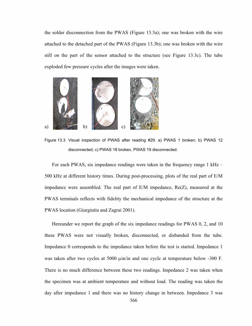
366
the solder disconnection from the PWAS (Figure 13.3a); one was broken with the wire
attached to the detached part of the PWAS (Figure 13.3b); one was broken with the wire
still on the part of the sensor attached to the structure (see Figure 13.3c). The tube
exploded few pressure cycles after the images were taken.
Figure 13.3 Visual inspection of PWAS after reading #29. a) PWAS 1 broken; b) PWAS 12
disconnected; c) PWAS 18 broken, PWAS 19 disconnected.
For each PWAS, six impedance readings were taken in the frequency range 1 kHz –
500 kHz at different history times. During post-processing, plots of the real part of E/M
impedance were assembled. The real part of E/M impedance, Re(Z), measured at the
PWAS terminals reflects with fidelity the mechanical impedance of the structure at the
PWAS location (Giurgiutiu and Zagrai 2001).
Hereunder we report the graph of the six impedance readings for PWAS 0, 2, and 10
these PWAS were not visually broken, disconnected, or disbanded from the tube.
Impedance 0 corresponds to the impedance taken before the test is started. Impedance 1
was taken after two cycles at 5000 μin/in and one cycle at temperature below -300 F.
There is no much difference between these two readings. Impedance 2 was taken when
the specimen was at ambient temperature and without load. The reading was taken the
day after impedance 1 and there was no history change in between. Impedance 3 was
a) b) c)

367
taken at about -270 F and after 3 cycles at about 6000 μin/in. Impedance 4 was taken
while the tank was filling with liquid nitrogen and without load. The reading was taken
the day after impedance 3. Impedance 5 was taken at the end of the test at room
temperature and with no load. The SHM system has withstood other 3 cycles with strain
above 6000 μin/in.
Figure 13.4 Impedance readings for PWAS 0
Figure 13.5 Impedance readings for PWAS 2 and 10
0
50
100
150
200
250
300
0 50 100 150 200 250 300
Impedance 0Impedance 1Impedance 2Impedance 3Impedance 4Impedance 5
Frequency (kHz)
Re
(z)
0
100
200
0 50 100 150 200 250 300
Imp 0 PWAS 02 Imp 1 PWAS 02Imp 2 PWAS 02 Imp 3 PWAS 02Imp 4 PWAS 02 Imp 5 PWAS 02Imp 0 PWAS 10 Imp 1 PWAS 10Imp 2 PWAS 10 Imp 3 PWAS 10Imp 4 PWAS 10 Imp 5 PWAS 10
Frequency (kHz)
Re
(z)

368
From Figure 13.4 and Figure 13.5, we can see that after the first two cycles at high
micro-strains, the SHM system reveals a new resonance frequency at about 100 kHz.
This resonance frequency is evident only when the structure is not subjected to load and
critical temperatures (impedance 2, 4, and 5). The same behavior can be seen in all the
PWAS that were still electronically connected.
While impedance results for 1 and 3 are similar to those of impedance 0, the baseline;
impedance 2, 4, and 5 show a new resonance frequency. The resonance frequency has
low energy for impedance 2, but it increases considerably in impedance 4 and 5. These
three readings have in common the environment and loading conditions. The tube is at
rest and the temperature has not reached the cryogenic level, the walls of the structure are
no more under tension. In previous studies (Giurgiutiu et al., 2003) we have seen that a
structural change in the substrate corresponds to knew frequency resonance in the
impedance spectrum. We could then link the new resonance frequency to a structural
change in the tube. For completeness of the exposure we should had analyzed the
quality of the bonding of the PWAS to the structure through microscope. However, the
PWAS were destroyed during the explosion of the tube.
Pith-catch data have been collected at two frequencies. The frequencies were
determined through tuning of the PWAS and the structure. We found experimentally that
we had maximum of the pseudo A0 mode at 45 kHz. For the pseudo S0 mode, we
selected the frequency, 165 kHz, at which the pseudo S0 mode is maximum and at the
same time the pseudo A0 mode and SH mode are minimum. Figure 13.6 shows the
readings we have analyzed. We discarded the readings from and to the PWAS that were
visually disconnected from the data acquisition system or those who were broken.

369
Figure 13.6 Post-processing analysis. Gray PWAS: transmitters; Black PWAS: bad wiring;
Arrows: pitch-catch direction, from the transmitter to the receiver.
We have noticed that when the tube is under high load levels and cryogenic
temperature, the pitch-catch analysis can not be performed (Figure 13.7) because the
wave amplitude is too attenuated and not visible.
Figure 13.7 Pitch-catch data at cryogenic temperature and strain level about 7000 μin/in.
Transmitter PWAS 4, receiver PWAS 11. Frequency 45 kHz.
V (m
V)
Time (μsec)
Readings 25 and 27
0 1 10 4−× 2 10 4−× 3 10 4−× 4 10 4−×
0.1
0.2
0.3
Readings 20 and 23
Readings 16 and 17

370
At ambient temperature and with the tube at rest and the wave propagating vertically
(towards the top or bottom) the first wave is almost coincident with the initial burst
because the wave speed is high (see Figure 13.8).
Figure 13.8 Pith-catch at ambient temperature and no load for PWAS 02 transmitter and PWAS
04 receiver (vertical wave propagation) at different history times. Frequency 45 kHz.
When we consider a pitch-catch along the horizontal direction, the wave speed
decreases considerably with respect to the vertical direction (-39%). When the pitch catch
is oblique, the wave speed decreases even more, but not so dramatically (-46%).
All the data analyzed appear qualitatively similar. Here we present only the case of
pitch-catch when PWAS 2 is transmitter and PWAS 10 and 12 are receiver. Figure 13.10
shows the wave propagating from PWAS 2 to PWAS 10, along the circumference. The
A0 mode is present for each reading, but the wave amplitude decreases as the number of
fatigue and thermal cycle increases. While the wave amplitude in the baseline reading
(Reading 0) is about 0.14 mV, in the last reading (Reading 29) the amplitude is about
-0.1
-0.06
-0.02
0.02
0.06
0.1
0 0 0 0 0 0 0 0 0 0 0 0 0 0 0 0 0 0 0 0
Reading 0Reading 11Reading 12Reading 28Reading 29
V (m
V)
Time (μsec)

371
0.07 mV. All the PWAS present the same kind of attenuation of the wave amplitude. This
can be due to either a structural change of the tube material or a degradation of the
PWAS capability to transmit-receive the signal. However, both pitch-catch signal and
impedance readings seem to be those of a healthy PWAS.
Figure 13.9 Pith-catch at ambient temperature and no load for PWAS 02 transmitter and PWAS
10 receiver (horizontal wave propagation) at different history times. Frequency 45
kHz.
Similar results are obtained considering a wave propagating obliquely with respect to
the circumference (Figure 13.11).
-0.1
-0.06
-0.02
0.02
0.06
0.1
0.00015 0.0002 0.00025 0.0003 0.00035
Reading 0Reading 11Reading 12Reading 28Reading 29
V (m
V)
Time (μsec)

372
Figure 13.10 Pith-catch at ambient temperature and no load for PWAS 02 transmitter and PWAS
12 receiver (oblique wave propagation) at different history times. Frequency 45 kHz.
At 165 kHz the wave amplitude is small. The noise to signal ratio is still low, hence it
is possible to recognize the same amplitude attenuation with the cycles as for the case of
45 kHz (Figure 13.11).
Figure 13.11 Pith-catch at ambient temperature and no load for PWAS 02 transmitter and PWAS
10 receiver (horizontal wave propagation) at different history times. Frequency 165
kHz.
-0.06
-0.02
0.02
0.06
0.1
0.00015 0.0002 0.00025 0.0003 0.00035
Reading 0Reading 11Reading 12Reading 28Reading 29
V (m
V)
Time (μsec)
-0.1
-0.06
-0.02
0.02
0.06
0.1
8.00E-05 1.00E-04 1.20E-04 1.40E-04 1.60E-04 1.80E-04 2.00E-04
Reading 0Reading 11Reading 12Reading 28Reading 29
V (m
V)
Time (μsec)

373
13.4 CONCLUSION
The SHM system installed on the tank tube was subjected to seven high strain cycles and
three cryogenic temperature cycles. At the end of the test, visual inspection was
performed. Five of the thirty-two PWAS installed were electronically disconnected, two
PWAS were broken. The PWAS proved to be working till the end of the catastrophic
experiment. The impedance readings show a new resonance peak at about 100 kHz, after
the first two cycles at high micro strains. It is not possible to asses with certainty whether
the new resonance is due to a structural change in the tube or to a PWAS – bond
degradation. However, the pitch-catch readings were consistent after different high load-
low temperature cycles, the new resonance peak of the impedance readings were at the
same frequency for all the connected PWAS (even the broken one PWAS 18), all these
seems to suggest a structural change in the tube under test. If this is the case, the PWAS
system have detected a structural change at history 22, after four high strains cycles and
three low temperature cycles. It is to be noted that however the standard SHM (ultrasonic
method) used to check the tube integrity did not reveal any damage in the structure.
The experiment conducted shown good survivability of the PWAS-bond system
either under harsh environmental condition (extreme temperature, aging, and liquid
contact) and extreme loads.

374
14 DURABILITY OF SHM SYSTEMS
To obtain space qualification, any non destructive evaluation methods must demonstrate
the durability of the system in different conditions. In Giurgiutiu (2004) and Giurgiutiu
and Lin (2004) have been presented initial durability and survivability tests - thermal
cycle loading, exposure to the environment, exposure to operational fluids such as oils,
hydraulics, fuels, etc.
In this Section we will present the durability of SHM through PWAS for space
applications.
14.1 REQUIREMENTS
For space certification of the NDE and health monitoring system, the entire SHM system
(hence transducer, bond layer, and wiring) must be subjected to durability test. From the
International Space Station Program (SSP) a summary of documents has been used to
provide requirements for the operating environment (thermal, acoustic, impact), hardware
selection, and system level integration (voltage drops, EMI). A notional test plan is
provided in Table 14.1.

375
Table 14.1 Notional test plan for space certification of NDE system
14.2 MISSION PROFILE
In order to obtain space qualification, tensile experiments on aluminum dog-bone bars
were performed to measure both the adhesive and PWAS strength. Data such as
impedance have been taken from the sensors at each static strain increment at cryogenic
temperature. The increments were of 250 μ strain up to 5,000 μ strain.
The specimen used was an aluminum dog bone beam. A PWAS was installed at the
middle of the dog bone while, on the other side, a strain gage was installed (Figure
14.1a).

376
Figure 14.1 Durability and survivability test. a) Specimen for durability and survivability test. b)
Durability setup.
In order to perform the test at cryogenic temperature under static load, a container for
nitrogen liquid as been fabricated. Figure 14.1b shows the dog bone specimen under
uniaxial load and at cryogenic temperature.
Figure 14.2 Impedance readings of PWAS at cryogenic temperature under uniaxial load
10
100
1000
0 50000 100000 150000 200000 250000 300000 350000 400000 450000 500000
0 us 500 us1000 us 1500 us2100 us 2500 us3100 us 4000 us5000 us
a) b)

377
From Figure 14.2 we can see that the bond quality did not change when the level
reached 5000 us and that it was possible to excite the PWAS at that level of strain.
14.3 SHOCK TEST
The ground handling shock test required that the system underwent a 20-g shock pulse in
both directions of each of the three orthogonal axes. A MTS 846 shock test system was
used for this test. It consisted of a drop table and a base with a pressurized cylinder. The
specimen used was the tank-dome joint as described in Figure 12.5, the experimental
setup is shown in Figure 14.3.
Figure 14.3 The dome-barrel specimen on the drop table. a) Transverse shock; b) In plane
shock.
An accelerometer was used to record the magnitude of the shock. A typical
accelerometer signal is shown in Figure 14.4. The drop test achieved a shock pulse that
was higher than 20-g’s meeting the requirement for the test.
b)a)

378
Figure 14.4 A typical accelerometer signal
To determine whether the SHM system survived the shock, a scan of the real part of
the impedance versus frequency was taken before and after the shock. Figure 14.5 shows
the graph of the real impedance versus frequency. Before and after scan, the impedance
does not differ, hence, no change in the SHM system has happened. The sensor network
can survive a 20-g shock pulse without sustaining damage.
Figure 14.5 The Re Z vs. Frequency before and after the test

379
14.4 RANDOM VIBRATION TEST
The objective of this test is to demonstrate system survivability of the sensor network
while it experiences vibrations similar to those on a launch vehicle. The required
spectrum is shown in Figure 14.6.
Figure 14.6 The required random vibration spectrum
A vibration exciter was used to complete this test. An accelerometer was used to
determine if the exciter could produce the needed amplitudes. The results of that test
showed that the exciter did not have the capability of producing the amplitudes required,
hence, the test was not performed.
14.5 THERMAL TEST
The thermal environment test requires that the thermal operating conditions of a
cryogenic tank be replicated to test for durability and survivability. Unlike the previous
two tests, the system must be operating while in this environment. To demonstrate that
the system can operate in this environment, an impact test was done on two different
specimens. Results are reported in Sections 12.3.3 and 12.3.4. The experiments
Vibration Spe ctrum
0.01
0.110 100 1000 10000
Frequency (Hz)
ASD
(g^2
/Hz)
Frequency (Hz) ASD (g2/Hz)
20 0.0125
20-50 +6 dB/oct
50-600 0.075
600-2000 -4.5 dB/oct
2000 0.0125
Overall 9.1 Grms b) a)

380
demonstrated that the sensors can not only survive the thermal environment but also
operate in this extreme environment, fulfilling the requirements for this test.
14.6 ACOUSTIC ENVIRONMENT TEST
The acoustic environment test mimics the acoustic noise environment experienced by the
structure of a launch vehicle. Figure 14.7a shows the required spectrum. During the test,
all the quoted sound energy levels are produced at the same time for the duration of an
actual launch, approximately three minutes.
Figure 14.7 Noise spectra. a) Required noise spectrum, b) Noise spectrum collected by a
microphone during the test
In Figure 14.7b is shown the recorded spectrum of the actual test. The recorded spectrum
met all the required sounds levels. A scan of the real impedance before and after the
exposure to acoustic environment was conducted. The scans recorded before and after the
acoustic test did not differ on a level that would indicate that damage was incurred. It can
be concluded that SHM system can withstand an acoustic environment experienced on a
launch vehicle.
b) a)

381
15 EFFECT OF PARTIAL BONDING BETWEEN TRANSDUCER AND
STRUCTURE ON CAPACITANCE
Structural health monitoring (SHM) methods are used to determine the health of a
structure. Transducers, attached to the surface of a structure, are used in a passive way
(listen to the structure) or in an active way (interrogate the structure). In our researches,
we use a particular kind of transducer called piezoelectric wafer active sensor (PWAS). A
network of PWAS is bonded through an adhesive layer to the structure. The sensor uses
the piezoelectric principle to convert a difference in voltage into a strain change. The
PWAS can be excited at different frequencies so that different modes of excitation are
activated.
The methods of interrogation of a structure through PWAS are pitch-catch, pulse-
echo, and electromechanical impedance (E/M). The latter method can be used also to
determine the quality of the bonding between the transducer and the structure.
Most of the applications for SHM are on structural components subjected to big
variation in the environment conditions (from high temperatures to cryogenic
temperatures (~-198 C)) and different strain levels (from 0 to 3000 μstrain). The structure
component, the PWAS, and the bonding layer have different thermal expansion
coefficients and different young modulus. They will stretch of a different amount and
under certain conditions the PWAS will disbond partially or fully from the structure. The
signal received by the half detached PWAS or fully detached PWAS is different from the

382
signal received when the PWAS is well attached. From the pitch-catch method or the
pulse-echo method it is not possible to determine whether the change in the signal is due
to damage in the structure or to a change in the conditions of the PWAS – structure
bonding.
The state of the art for this technique is that if a transducer is well bonded to the
structure, the E/M reading shows suddenly change in the real impedance amplitude and a
discontinuity of the imaginary impedance at the resonance frequency of the structure
(Giurgiutiu, 2008). The impedance spectrum of a PWAS with free boundary conditions
presents a resonance at 296 kHz that it is not present when the PWAS is attached to a
structure (Giurgiutiu, 2008). However, we do not know how the impedance spectrum
changes when the PWAS bonding degrades and the PWAS becomes partially attached to
the structure or totally detached but without free boundary conditions. Moreover, it is
difficult to define a general procedure to ensure debonding detection of the transducers
through E/M.
A more easy way to determine the quality of the bonding is through capacitance. We
know that a well bonded PWAS has a capacitance value of about 2.67 nF. However, we
do not know how different it is the capacitance of a partially detached PWAS or of a
detached one.
In the present section we will try to establish how it is possible to determine if a
PWAS is well bonded or not through capacitance method.
Future SHM technique will integrate the use of capacitance check when variations in
pitch-catch, or pulse-echo, or E/M values are found during data collection. If the
capacitance of the transducers has changed to a degree that is evidence of bonding

383
degradation, the change in the SHM readings will be disregarded and a false call for
damage in the structure will be avoided.
The experiment performed had one factor with three levels (a: fully bonded, b: half
bonded, c: not bonded). The response we were interested in was the capacitance variation
and of the structure (PWAS + strip of metal).
The experimental unit is a PWAS attached to the structure. We will use identical
strips of Aluminum metal 160x50x1 mm. On each strip, 6 PWAS are installed (see
Figure 15.1).
Figure 15.1 Specimen with PWAS installed (A – F: PWAS location)
The position of the PWAS on the strip can affect the results recorded; we will
randomize the PWAS location on the strip.
15.1 POWER ANALYSIS AND SAMPLE SIZE
We performed a power analysis to check that the experiment setup was sufficient to
guarantee a power of 0.8 for an alpha level of 0.05. We used SAS to determine the power
as described in Gatti et al. (1998). The SAS program used was:
A B C A B C

384
PROC IML;
F = FINV(PR, DF1, DF2, 0);
POWER = 1 - PROBF(F, DF1, DF2, NCP);
PRINT 'F VALUE = ' F;
PRINT 'POWER = ' POWER;
Where DF1 is the numerator degrees of freedom (r-1), DF2 was the denominator
degrees of freedom (rn-r), n was the number of replication per cell, PR = 1-α, and NCP
= λ represented the non centrality parameter. We could find λ from the relation
2 2k
k nλτ σ =∑ , where k kτ μ μ= −
In order to determine the power, we should know the variance of the experiment and
the value of the response difference that determines our rejection region. In order to
proceed we need an estimation of the variance.
15.2 POPULATION VARIANCE
To obtain the variance of the test we performed a preliminary investigation of the
variance of the response on PWAS already installed on different specimens. We took in
consideration PWAS installed on specimens with same thickness and dimensions and
attached with the same adhesive. For this purpose, we used PWAS already installed on
specimens available in our laboratory. From this preliminary experiment it was possible
not only to estimate the variance but also to estimate 2k
kτ∑ .
We measured the capacitance of 24 PWAS installed on different plates. Results of the
preliminary experiment are reported in Table 15.1.

385
Table 15.1 Capacitance variance.
Capacitance (nF)
Mean Variance
2k
kτ∑ 2 2
kk
τ σ∑
2.679 0.0155 0.358 23
Table 15.2 reports the different values of power we obtain for different values of n.
Table 15.2 Power as a function of n for 3r = , 0.05α = .
n 2 2k
knλ τ σ= ∑ Power (from SAS)
2 46 0.917
3 69 0.999
4 92 1
We can obtain a high value of power (~0.92) with n = 2, r = 3, α = 0.05.
15.3 EXPERIMENTAL SETUP
The experiment setup is reported in Table 15.3, where a represents the PWAS full
bonded, b represents the PWAS partially bonded, and c represents the PWAS detached
(see Figure 15.1). Capital letters A, B, and C represent PWAS location on the specimen
as described in Figure 15.1. There are a total of 18 PWAS (6 for each factor level, 6 for
each strip and 3 for each location).
Table 15.3 Experiment setup. 1 – 3: specimen identification number; a – c: type of bonding
Location
A B C C B A
1 a b c c b a
2 c a b b a c
Spec
imen
3 b c a a c b

386
Because factor level c is a PWAS wired but detached from the structure, it can
happen that the PWAS is not in contact with the structure. In order to avoid this case, we
taped the PWAS to the structure. This reflected realistic environment conditions. Real
structures are often in contact with other foam layers for thermal insulation and or
protection. A piece of tape will be applied to all PWAS used in the experiment.
15.4 EXPERIMENT
The PWAS were installed by the same operator. The procedure to install PWAS in
configuration a was the standard procedure used to install strain gages:
1. sand
2. apply conditioner
3. apply neutralizer
4. apply catalyst
5. apply adhesive (M-bond 200)
6. hold the PWAS under pressure with the finger for 90 sec.
The procedure to install PWAS in configuration b was the same as that for PWAS in
configuration a. To obtain partial bonding, a piece of tape was applied on the bottom half
of the sanded surface (Figure 15.2 b). The part of surface under the tape was not cleaned
as required and we did not apply catalyst to it (Figure 15.2 c-e). A small amount of glue
was applied only on the top half of the surface (Figure 15.2 f). After we had applied the
glue we removed the tape and pressed the PWAS on the surface such that the excessive
amount of glue would follow the arrow direction in Figure 15.2 g.

387
Figure 15.2 Installation procedure for configuration b
We tested the installation procedure on an aluminum plate. We were able to obtain
partially bonded PWAS, but the amount of surface not bonded was not constant. Small
variation in adhesive would lead to big difference in bonding extension. However, this
was considered to be the most reliable and consistent method to obtain partially bonded
PWAS. At the end of the experiment, we will destroy the PWAS in configuration b to
check the extension of the bonding.
After the installation, we recorded the capacitance value of the PWAS. Table 15.4
reports the findings. As we can see, the PWAS not bonded present higher capacitance
while the PWAS full bonded present the lower values of capacitance. PWAS in
configuration b have capacitance that varies form the higher values of PWAS in
Sand
Tape
Conditioner
Neutralizer a) b) c)
d) e) f)
PWAS
g)
Catalyst
M bond 200

388
configuration a to the lower values of PWAS in configuration c. Configuration b presents
the highest standard deviation.
Table 15.4 Capacitance (nF) of the PWAS
Specimen
1 2 3 mean std
a 2.65 2.72 2.70 2.68 2.69 2.69 2.69 0.02
b 2.89 2.81 3.13 2.99 3.09 2.80 2.95 0.14
c 3.31 3.25 3.32 3.32 3.27 3.24 3.28 0.04
We inspect the PWAS in configuration b. We found that the PWAS with a smaller
amount of adhesive around the edge of the transducer had smaller capacitance, while a
less amount of adhesive around the edge corresponded to a higher capacitance. Figure
15.3 shows an example of this situation. The dark gray shadow around the PWAS is the
hardened glue. PWAS b on specimen #3 has a smaller shadow and it is all located in the
upper part of the PWAS itself. PWAS b on specimen #5 has a small shadow but it is
almost all around the PWAS. If we compare their capacitance we see that PWAS b on
specimen #3 has a higher capacitance (2.80 nF) than PWAS b on specimen #5 (2.67 nF).
Figure 15.3 PWAS bonded to specimen #3. PWAS in configuration b has a less amount of glue
than that of PWAS in configuration a. The capacitance is 2.80 nF and 2.69 nF
respectively.

389
15.5 ANALYSIS
In order to perform the analysis, we must check the assumptions. We found that the
normality assumption is not completely met.
-2 -1 0 1 2
-1. 500E-01
-1. 000E-01
-5. 000E-02
0
5. 0000E-02
1. 0000E-01
1. 5000E-01
resid
Normal Quant i l es
Figure 15.4 QQ-plot and residual plot
From the plot of the residual we checked that the variance of the residuals was
constant.
Figure 15.5 show the interaction plots between the bond type (a = full bonded, b =
partially bonded, c = detached) and respectively PWAS location and the specimen. From
the plots we deduce that there is no interaction between the factor bond and the blocks
specimen and location.

390
Figure 15.5 Interaction plots. a) Interaction between PWAS location and bond type. b)
Interaction between specimen and bond type.
We perform the analysis of the latin square with replications within the cell with the
PROC GLM function in SAS. The SAS program use was:
Proc glm;
class Spec Loc Bond;
model Cap=Spec Loc Bond;
run;
The output is:
Source DF Type III SS Mean Square F Value Pr > F
Specimen 2 0.0229 0.01145 1.89 0.1968
Blocks
Location 2 0.0190 0.00951 1.57 0.2509
Factor Bond 2 1.0729 0.53646 88.63 <0.0001
Cap1
2. 6
2. 7
2. 8
2. 9
3. 0
3. 1
3. 2
3. 3
3. 4
1 2 3
B
B
B
C
C
C
B C
Bond: a, b, c
Location
3.4 3.3 3.2 3.1 3.0 2.9 2.8 2.7 2.6
A
p1
6
7
8
9
0
1
2
3
4
1 2 3
B
B
B
C
C
C
2 3
Specimen
1
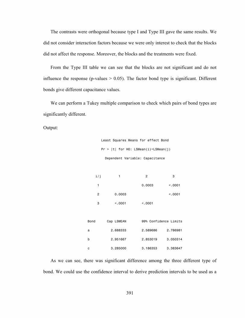
391
The contrasts were orthogonal because type I and Type III gave the same results. We
did not consider interaction factors because we were only interest to check that the blocks
did not affect the response. Moreover, the blocks and the treatments were fixed.
From the Type III table we can see that the blocks are not significant and do not
influence the response (p-values > 0.05). The factor bond type is significant. Different
bonds give different capacitance values.
We can perform a Tukey multiple comparison to check which pairs of bond types are
significantly different.
Output:
Least Squares Means for effect Bond
Pr > |t| for H0: LSMean(i)=LSMean(j)
Dependent Variable: Capacitance
i/j 1 2 3
1 0.0003 <.0001
2 0.0003 <.0001
3 <.0001 <.0001
Bond Cap LSMEAN 99% Confidence Limits
a 2.688333 2.589686 2.786981
b 2.951667 2.853019 3.050314
c 3.285000 3.186353 3.383647
As we can see, there was significant difference among the three different type of
bond. We could use the confidence interval to derive prediction intervals to be used as a

392
rule to check the goodness of the bonding. We can say that we are 99% confident that a
PWAS well bonded has a capacitance value between 2.58 nF and 2.78 nF.
From theses results, we concluded that capacitance methods can be an effective tool
to use along with SHM method to check whether a detection of damage was due to a real
damage or a change in the transducer bonding quality (true call or false call). From the
analysis above we derived 99% confidence interval that could be used to derive the
reference values to determine the status of the bonding between transducer and structure.
The analysis we performed had as assumption the normality of the data. This assumption
was not completely met, hence the CI interval we derived were not to be trusted
completely. For further analysis, a non parametric model should be taken into account to
verify the goodness of the CI derived in this section.

393
16 GUIDED WAVES SCATTERING FROM DAMAGE
Lamb waves scattering from a defect has been studied through Mindlin theory or through
boundary element model, finite difference model and finite element model. The problem
under investigation has complex wave interactions and usually complex geometries,
hence numerical methods represent the only viable approach for understanding the
multiple reflections and diffractions of the ultrasonic waves within the component. Most
of the work done to date is on circular holes or defects with a regular shape. Among the
few papers on wave scattering from crack, Messerery et al. (2005) focused on Rayleigh
wave propagation.
Lamb waves excited in a plate have more then one mode of propagation. When the waves
interact with a defect in the structure the waves are modified by mode conversion.
Therefore, the received signal generally contains more than one mode, and the
proportions of the different modes present is modified by mode conversion at defects and
other impedance changes. The wave modes are also generally dispersive, which means
that the shape of a propagating wave changes with distance along the propagation path.
When mode conversion took place, the geometry of the structure under consideration is
important. If the geometry of the structure is symmetric, only the same family modes as
an incident mode are capable of carrying each portion of scattered energy, so if the
incident wave is antisymmetric one, there is no chance that the reflection of S0 mode
could occur. The incident wave mode and the converted wave mode overall must have

394
the inverse trend to the other, satisfying the energy conservation. This is because each of
those scattered modes would share its own portion of scattered energy with the other
mode through mode conversion, based on a fixed amount of incident energy.
In order to perform health monitoring it is important to decide which mode(s) and
frequency of the excitation to use. The sensitivity of different modes in different
frequency-thickness regions is a parameter that enables to determine the best testing
regime for a particular type of defect. The S0 mode at low frequencies has the
characteristic of low dispersion and low leakage of energy if the plate is fluid loaded;
moreover, the stresses due to S0 mode are almost uniform through the thickness of the
plate so that its sensitivity to a defect is not dependent on the through the thickness
location of the defect. Lowe et al. (2002) and Alleyne et al. (1992) studied the Lamb
wave scattering from a notch through finite element simulations.
Lowe et al. (2002) studied through finite element model the reflection of Lamb mode S0
from a rectangular notch in a plate. The notch is assumed to be rectangular in section
(with zero width in the case of a crack), to be infinitely long and aligned normal to the
direction of wave propagation. Lowe also assumed plane strain in the plane of the particle
motion of the Lamb wave. The displacement in the in-plane direction was monitored at
the mid-thickness of the plate, thus ensuring that only the symmetric S0 propagating
mode was detected, since the antisymmetric A0 mode has zero in-plane displacement at
this depth.
An alternative to finite element model are the boundary element model. This method
seems to be a powerful tool for describing Lamb wave mode conversion phenomena from
an edge. Cho et al. (1996) used the boundary element method to study the mode

395
conversion phenomena of Lamb waves from a free edge. They applied their method to
the study of multimodes reflection from free edge in a semi-infinite steel plate. They
found that S1 is the mode which is less affected by the other modes’ appearance in mode
conversion. Cho (2000) also studied the mode conversion in a plate with thickness
variation through the hybrid boundary element method. The elastodynamic interior
boundary value problem is formulated as a hybrid boundary integral equation in
conjunction with the NME technique based on the Lamb wave propagation equation.
Vermula and Norris (2005) studied flexural wave scattering on thin plates using Mindlin
theory. Also McKeon et al. (1999) and Hinders (1996) used the Mindlin theory to study
Lamb waves scattering from a through hole and rivets, respectively. Mindlin theory
includes shear-deformation and rotary-inertia effects, as in the Timoshenko beam theory.
The equations of motion restrict the deformation to three degree of freedom, and they are
obtained by averaging the exact equations of elasticity across the plate thickness.
Grahn (2002) used a 3D approach to studied the scattering problem of an incident plane
S0 Lamb wave in a plate with a circular partly through-thickness. The wave fields in the
outer part outside the hole and in the inner part beneath the hole are expanded in the
possible Lamb modes and the horizontally polarized shear modes. Both propagating
modes and evanescent modes were included in the expansions. The expansion
coefficients were obtained by utilizing the boundary conditions at the hole boundary and
the continuity conditions below the hole. He derived a linear system of equations for the
expansion coefficients by projecting the different boundary conditions onto an orthogonal
set of projection functions.

396
Moreau et al. (2008) extended the 3D approach to more complex geometry through the
use of both orthogonality relations and finite element modes.
In the method presented the scattering coefficient of Lamb waves generated by the
interaction of incident wave with scatterers in a plate were directly determined by using a
FEM or a BEM in conjunction with normal mode expansion. Gunawan et al. (2004)
proposed a mode-exciting method where all Lamb modes are simultaneously excited by
appropriate boundary conditions given on both ends of a finite plate. The excited Lamb
wave modes constitute a system of equations which is solved to determine the scattering
coefficients for all Lamb modes.
Hereunder we report a preliminary modeling of Lamb waves scattering from a sudden
change in material properties in the plate and SH waves scattering from a crack on a
plate.
In this section, we present some preliminary modeling of Lamb waves and SH waves
scattering from inhomogeneity and damage following Ditri (1996). First, we extend the
derivation made by Ditri for SH waves to the case of a non-through the thickness crack in
the plate. Second, we present the generic derivation of Lamb waves scattering when a
difference in both thickness and material properties is encountered by a propagating
wave.
16.1 MODE DECOMPOSITION OF INCIDENT, REFLECTED, AND TRANSMITTED WAVES:
SH WAVES SCATTERING FROM A CRACK
Consider a plate of thickness d with a crack of depth 1d as depicted in Figure 16.1. For
convenience with consider the plate as formed of two plates 0Ω and 1Ω of same

397
thickness and material properties perfectly joined at the boundary region Γ (dash line in
Figure 16.1).
Figure 16.1 Plate with a crack depth 1d .
The particle displacement field is only in the z direction and it is denoted with 0zu for
region 0Ω and 1zu for region 1Ω . The particle displacement field must satisfy the equation
of motion in Equation (3.5) for SH waves under the assumption of external forces equal
to zero, i.e.,
2 2 2
2 2 2z z zu u u
x y tρμ
∂ ∂ ∂+ =
∂ ∂ ∂ (16.1)
The displacement fields can be expressed as a summation of all the positive and negative
travelling or decaying normal modes, i.e.,
( )( , , ) ( )n ni x i x i tz n n zn
nu x y t a e b e u y e
α αξ ξα α α α ω−= +∑ (16.2)
where { }0,1α ∈ ; the terms with amplitude nza represent the positive travelling or
decaying modes for the displacements in the z direction; the terms with amplitude nzb
represent the negative travelling or decaying modes for the displacements in the z
direction. The modes are traveling if nξ is real or decaying if nξ is imaginary. The sign
of the wavenumber is taken into account in the exponential term.
0Ω
1ddΓ
x
y
1Ω
Crack

398
Each term in Equation (16.2) must satisfy the third equation in (16.1) provided
( )
222
2
222
2
symmtric modes
2 1 antisymmtric modes2
s
s
nc d
nc d
ω πξ
ω πξ
⎛ ⎞= − ⎜ ⎟⎝ ⎠
⎛ ⎞+= − ⎜ ⎟
⎝ ⎠
(16.3)
The terms in Equation (16.2) must satisfy the traction-free boundary conditions at the
upper and lower surfaces of each semi-plate, i.e.,
0
0
0
0
zyz y
y
zyz y d
y d
uTy
uTyα
μ
μ
==
==
⎧ ∂= =⎪ ∂⎪
⎨∂⎪ = =⎪ ∂⎩
(16.4)
In addition, we must impose continuity of displacements and stresses at the common
boundary Γ , i.e., for the displacements using Equation (16.2)
( ) ( )0 0 0 1 1 1( ) ( )n n nz n n nzn n
a b u y a b u y+ = +∑ ∑ (16.5)
The non zero tractions at the boundary Γ is xzT given by
zxz
uTx
α
μ ∂=
∂ (16.6)
Requiring continuity at Γ leads to
0 10 0xz xzx x
T T= =
= (16.7)
or, by substituting Equation (16.2) into (16.7) and after rearrangement
( ) ( )0 0 0 0 1 1 1 1( ) ( )n n n zn n n n znn n
a b u y a b u yξ ξ− + = − +∑ ∑ (16.8)

399
Last condition to be satisfied is that the portion of the plate at the crack interface be
traction-free, hence
0
00
110
0 \
0 \xz x
xz x
T y
T y=
=
= ∈∂Ω Γ
= ∈∂Ω Γ (16.9)
where 0∂Ω is the right boundary of 0Ω and 1∂Ω is the left boundary of 1Ω . With the use
of Equation (16.2), Equation (16.9) becomes
( )
( )
0 0 0 00
1 1 1 11
( ) 0 \
( ) 0 \
n n n znn
n n n znn
a b u y y
a b u y y
ξ
ξ
− + = ∈∂Ω Γ
− + = ∈∂Ω Γ
∑
∑ (16.10)
Consider the case in which a single propagating Lamb waves mode m is generated in
plate 0Ω with unit amplitude and propagating in the positive x direction. Hence, we
impose the following conditions
0
1 0n nm
n
a
b
δ=
= (16.11)
where nmδ is the delta Kronecker. Substitution of Equation (16.11) into Equations (16.5),
(16.8), and (16.10) yields after rearrangement
0 0 1 1 0( ) ( ) ( )n nz n nz mzn n
b u y a u y u y− = −∑ ∑ (16.12)
0 0 0 1 1 1 0 0( ) ( ) ( )n n zn n n zn m zmn n
b u y a u y u yξ ξ ξ+ =∑ ∑ (16.13)
0 0 0 0 00
1 1 11
( ) ( ) \
( ) 0 \
n n zn m zmn
n n znn
b u y u y y
a u y y
ξ ξ
ξ
= ∈∂Ω Γ
= ∈∂Ω Γ
∑
∑ (16.14)

400
To solve this problem, assume that there are N modes reflected and N modes transmitted.
The total numbers of unknown are 2N, hence to solve this problem we need 2N number
of equations. For each y ∈Γ two equations are created; continuity of displacements and
stresses, Equations (16.12) and (16.13). For each 0y δ∈ Ω Γ one equation is created,
stress-free boundary, first equation of (16.14). For each 1y δ∈ Ω Γ one equation is
created, stress-free boundary, second equation of (16.14). We apply the interface
conditions (16.12) and (16.13) at k points ky ∈Γ and the stress-free conditions at k points
ky αδ∈ Ω Γ , giving a total of 4m equations. To be able to solve the equations we must
have 4m=2N.
The system of equations can be written as
[ ]{ } { }A x b= (16.15)
where { } { }0 1 1 0 1 1, , , , , , , Tk kx b b b a a a− −= K K is the column vector of amplitude reflection
and transmission factors; the square [ ]A matrix is given by
( )
( )
( )
( )
( )
( )
0, 1
1, 1
0 0, 1
1 1, 1
0 02 , 1
2 ,
3 ,
1 13 , 1
( )
( )
( )
( )
( )
0
0
( )
i j ij z
i j N ij z
i k j n ij z
i k j N n ij z
i k j n i kj z
i k j N
i k j
i k j N n i kj z
A u y
A u y
A u y
A u y
A u y
A
A
A u y
ξ
ξ
ξ
ξ
−
+ −
+ −
+ + −
+ +−
+ +
+
+ + +−
=
= −
=
=
=
=
=
=
(16.16)
vector { }b is given by

401
0
0 0
0 02
3
( )
( )
( )0
i mz i
i k m mz i
i k m mz i k
i k
b u y
b u y
b u yb
ξ
ξ+
+ +
+
= −
=
==
(16.17)
Consider a 10-mm plate with a crack of depth d1=3/5d. Figure 16.2 shows the particle
displacement of the incident, reflected, and transmitted wave.
Figure 16.2 Particle displacement of the incident, reflected, and transmitted SH0 wave at f=1000
kHz. a) Distance from the crack x=2 mm; b) Distance from the crack x=5 mm.
The plots were computed retaining 238 modes for each wave. The incident SH0 wave is
symmetric and so it is the transmitted wave. The reflected wave amplitude is greater in
the region of the thickness where the crack is present. For a thoroughly analysis, we
should derive the energy of the three waves and evaluate the error made in the
assumption.
200− 0 200 400
2
4
6
8
10
100− 0 100 200 300 400
2
4
6
8
10
y
uz/βm uz/βm a) b)
Transmitted
Reflected
Incident Crack

402
16.2 MODE DECOMPOSITION OF INCIDENT, REFLECTED, AND TRANSMITTED WAVES:
LAMB WAVES SCATTERING FROM CHANGE IN MATERIAL PROPERTIES
Consider two semi-infinite flat layers of isotropic material as depicted in Figure 16.1
perfectly joined at the common boundary Γ .
Figure 16.3 Two semi-infinite layers with different thickness and material properties. (After Ditri,
1996)
The two layers denoted by regions 0Ω and 1Ω can have different thickness and material
properties. The particle displacement fields are denoted as 0xu , 0
yu , and 0zu for region 0Ω
and 1xu , 1
yu , and 1zu for region 1Ω . The particle displacement fields must satisfy the
equations of motion in Equation (3.5) under the assumption of external forces equal to
zero, i.e., Equation Chapter 13 Section 1
( ) ( )
( ) ( )
22 2 2
2 2 2
2 2 22
2 2 2
2 2 2
2 2 2
2
2
yx x x
y y yx
z z z
uu u ux y x y t
u u uux y x y t
u u ux y t
αα α α
α α αα
α α α
λ μ μ λ μ ρ
λ μ μ λ μ ρ
μ μ ρ
⎧ ∂∂ ∂ ∂+ + + + =⎪
∂ ∂ ∂ ∂ ∂⎪⎪ ∂ ∂ ∂∂⎪ + + + + =⎨ ∂ ∂ ∂ ∂ ∂⎪⎪ ∂ ∂ ∂
+ =⎪∂ ∂ ∂⎪⎩
(16.18)
where { }0,1α ∈ .
0Ω 1Ω0d 1dΓ
x
y

403
Consider the equation of motions for Lamb waves propagating in an isotropic plate. The
displacement fields in each region can be expressed as a summation of all the positive
and negative travelling or decaying normal modes, i.e.,
( )
( )( , , ) ( )
( , , ) ( )
n n
n n
i x i xn n n i tx x x x
n
i x i xn n n i ty y y y
n
u x y t a e b e u y e
u x y t a e b e u y e
α α
α α
ξ ξα α α α ω
ξ ξα α α α ω
−
−
= +
= +
∑
∑ (16.19)
where the terms with amplitude nxa and n
ya represent the positive travelling or decaying
modes for the displacements in the x and y direction respectively; the terms with
amplitude nxb and n
yb represent the negative travelling or decaying modes for the
displacements in the x and y direction respectively. The mode will be traveling if nξ is
real or decaying if nξ is imaginary. The sign of the wavenumber is taken into account in
the exponential term.
Each term in Equation (16.19) must satisfy the first two equations in (16.1) provided that
the wavenumbers are solution of the Rayleigh Lamb waves Equations (3.20) and (3.21).
The terms in Equation (16.19) must satisfy the traction-free boundary conditions at the
upper and lower surfaces of each semi-plate, i.e.,
( )
( )
00
00
2 0
2 0
0
0
yxyy y
y
yxyy y d
y d
yxxy y
y
yxxy y d
y d
uuTx y
uuTx y
uuTy x
uuTy x
αα
αα
α
α
α
α
λ λ μ
λ λ μ
μ
μ
==
==
==
==
⎧ ∂⎡ ⎤∂= + + =⎪ ⎢ ⎥∂ ∂⎣ ⎦⎪
⎪ ∂⎡ ⎤∂⎪ = + + =⎢ ⎥⎪ ∂ ∂⎣ ⎦⎪⎨
∂⎛ ⎞∂⎪ = + =⎜ ⎟⎪ ∂ ∂⎝ ⎠⎪⎪ ∂⎛ ⎞∂⎪ = + =⎜ ⎟∂ ∂⎪ ⎝ ⎠⎩
(16.20)

404
We must impose continuity of displacements and stresses at the common boundary Γ ,
i.e., for the displacements using Equation (16.19)
( ) ( )
( ) ( )
0 0 0 1 1 1
0 0 1 1
( ) ( )
( ) ( )
n n n n n nx x x x x x
n n
n n n n n nx x y x x y
n n
a b u y a b u y
a b u y a b u yα α
+ = +
+ + +
∑ ∑
∑ ∑ (16.21)
The non zero tractions at the boundary Γ are xxT and xyT given by
( )2 yx
xx a
yxxy
uuTx y
uuTy x
αα
α γ
αα
α
λ μ λ
μ
⎧ ∂∂= + +⎪
∂ ∂⎪⎨
⎛ ⎞∂∂⎪ = +⎜ ⎟⎪ ∂ ∂⎝ ⎠⎩
(16.22)
Requiring continuity at Γ leads to
0 1
0 0
0 1
0 0
xx xxx x
xy xyx x
T T
T T= =
= =
⎧ =⎪⎨
=⎪⎩ (16.23)
or, by substituting Equation (16.19) into (16.23) and after rearrangement
( ) ( ) ( )
( ) ( ) ( )
( ) ( )
( ) ( )
00 0 0 0 0 0
0 0 0
11 1 1 1 1
1 1 1
00 0 0 0 0 0
11 1 1 1 1 1
( )2 ( )
( )2 ( )
( ) ( )
( ) ( )
nyn n n n n
n x x x y yn n
nyn n n n n
n x x x y yn n
nn n n n nxx x n y y y
n n
nn n n n nxx x n y y y
n n
u yi a b u y a b
yu y
i a b u y a by
u ya b i a b u yy
u ya b i a b u yy
α
ξ λ μ λ
ξ λ μ λ
ξ
ξ
∂+ − + + + =
∂
∂= + − + + +
∂
∂+ + − + =
∂
∂= + + − +
∂
∑ ∑
∑ ∑
∑ ∑
∑ ∑
⎧⎪⎪⎪⎪⎪⎨⎪⎪⎪⎪⎪⎩
(16.24)
Last condition to be satisfied is that the portion of the thicker plate that extends below the
interface region must be traction-free, hence

405
1
011
0
0 \
0xx x
xy x
Ty
T=
=
⎧ =⎪ ∈∂Ω Γ⎨=⎪⎩
(16.25)
where 1∂Ω is the left boundary of 1Ω . With the use of Equation (16.19), Equation
(16.25) becomes
( )1 1 1 1
1 1 1
111 1 1 1
2 0 \
0
nyn n n
n x x yn n
nn n nxx n y y
n n
ui a u a
yy
ua i a uy
α
ξ λ μ λ
ξ
⎧ ∂− + + =⎪
∂⎪ ∈∂Ω Γ⎨∂⎪ − =⎪ ∂⎩
∑ ∑
∑ ∑ (16.26)
Consider the case in which a single propagating Lamb waves mode m is generated in
one of the two layers 0Ω with unit amplitude and propagating in the positive x direction.
Hence, we impose the following conditions
0 0
1 1 0
n nx y nm
x y
a a
b b
δ= =
= = (16.27)
where nmδ is the delta Kronecker. Substitution of Equation (16.27) into Equations(16.21),
(16.24), and (16.26) yields
0 0 0 0 1 1
0 0 0 1
( ) ( ) ( )
( ) ( ) ( )
m m n n n nx x x x x x
n nm m n n n ny y x y x y
n n
a u y b u y a u y
a u y b u y a u yα α
+ =
+ +
∑ ∑
∑ ∑ (16.28)
( )
( )
0 00 0 0 0 0 0 0
0 0 0
11 1 1 1
1 1 1
0 0 10 0 0 0 0 0 0 0 1 1 1 1
2
2
m ny ym m n n m n
n x x x x y yn n
nyn n n
n x x yn n
m n nm n m m n n n n nx x xx x n y y n y y x n y y
n n n n
u ui a u b u a b
y y
ui a u a
yu u ua b i a u i b u a i a uy y y
ξ λ μ λ
ξ λ μ λ
ξ ξ ξ
⎧ ⎡ ⎤∂ ∂⎡ ⎤+ − + + + =⎪ ⎢ ⎥
∂ ∂⎢ ⎥⎣ ⎦ ⎣ ⎦⎪⎪ ∂⎪= − + +⎨ ∂⎪⎪ ∂ ∂ ∂
+ − + = −∂ ∂ ∂
⎩
∑ ∑
∑ ∑
∑ ∑ ∑ ∑⎪⎪
(16.29)

406
( ) ( )
( ) ( )
1 1 11 1 1
111 1 1 1 1 1
2 0 \
0
n n
nyi x i xn n n n
n x x y yn n
nn n n n nxx x n y y y
n n
ui a u a e b e
yy
ua b i a b uy
α αα
ξ ξα αξ λ μ λ
ξ
−⎧ ∂+ + + =⎪
∂⎪ ∈∂Ω Γ⎨∂⎪ + + + =⎪ ∂⎩
∑ ∑
∑ ∑ (16.30)
Solution for the Lamb waves mode is not straight forward as for the SH waves case even
if we consider the simple case of equal thickness but different material. The intent of this
section was to formulate the problem, but no solution is derived.

407
17 ACOUSTIC EMISSION IN INFINITE PLATE
Acoustic emission (AE) is a phenomenon arising from a rapid release of strain energy
within a material. This can due to a crack propagating or an object impacting the
structure. PWAS transducers can be used either as active sensors to interrogate the health
of the structure on demand or as passive sensors that listens for AE. In AE this energy
radiates from the source in the form of elastic waves. The response is principally affected
by the angular direction of the force and the distance between source and response.
Acoustic emission have been studied extensively, the angular direction of the force
has been studied experimentally by Prosser (1991) and Gorman et al. (1991). They
measured the out of plane displacement of the wave with force angle with respect to the
surface varying from 90 to 0 with steps of 30 degrees. To catch the response when the
force was at 0 degree, the transducer was located not on the surface of the pate but on the
edge of it. They noticed that vertical forces gave larger flexural waves while horizontal
forces gave larger longitudinal waves. This led the authors to assume that the relative
amplitude could give information about source orientation. However, this was not
proven.
It was also found that the distance between the receiver and the source affects the
response by changing the sign of the response. If the antisymmetric mode of the structure
has been excited, the response will be antisymmetric, and the sign of the displacement
will change as the distance between the source and the receiver changes.

408
Another interesting founding was made by Pao et al. (1979) (ray theory). The location
of the source and receiver with respect to the surfaces of the plate varies the response. In
particular, the authors found that it would be difficult to distinguish the response due to
the configuration with source in the middle of the plane or source on the surface and
receiver on the opposite surface. A third configuration, with both source and receiver on
the same surface, is instead significantly different from that of the buried force because
the Rayleigh wave is now present in the response.
Medick (1961) and Gorman et al. (1990) developed a method to simulate AE called
normal mode solution for classic plate theory. This method is based on the approximate
solution for flexural plate mode and low frequency assumption. The out-of-plane
displacement is modeled through the classic plate theory in which the in-plane
displacements are neglected and a shear coefficient is taken into account to introduce the
shear effect. This method is suited for thin homogeneous isotropic plates. The load is
assumed to be concentrated in one point and normal to the surface. If we further assume
that the load can be expressed as ( )Pf t , the model for the acoustic emission is
represented as
4 ( ) ( )( , ) ( , )2
Pf t rD w r t hw r trδρ
π∇ + =&& (17.1)
where w is the displacement in the out-of-plane direction, D is the flexural plate
stiffness, and ρ is the material density.
This method is quite simple to implement. A Matlab program has been written in our
lab, this program can compute the out-of-plane displacement recorded by the transducers

409
for a given plate dimensions, source and receiver location. Our transducer however can
sense the in-plane displacements, hence this model is not useful for our applications.
Two different methods have been developed so far that are able to model in-plane
displacements.
Pao et al. (1979) and Pao (1978) have studied transient wave in elastic plate through
the generalized ray solution. The solution is derived for any mode present and it can be
applied for thick or thin plates, however, the plate must be assumed to be infinite. The
model will derive the exact solution as long as the time duration it is modeled is
sufficiently small. The load configuration can be that of a concentrated force, a double
force on any surface of the plate, or a dilatation force.
The solution is derived by summing the contribution due to all possible reflections of
a wave from the source to the receiving point (see Figure 17.1). The model is based on
the generalized ray solution in which a generalized path is specified by the path along
which the wave propagates and by the modes of the wave motion. The modes considered
are that of a pressure or a shear wave. For a given source and receiver point in the plate,
an infinite number of paths can be drawn. The greater the number of paths is taken in
consideration the longer the time interval that the model can predict. Figure 17.2 shows
the theoretical derivation for a plate of thickness h with a force normal to the bottom
surface and a receiver in the top surface at distance 4h from the force in the r direction.
As the bold arrow in the simulation graphs denotes the time beyond which the results are
no more exact. Note that the complexity of the derivation increases rapidly with the
number of paths.

410
Figure 17.1 Generalized rays from a source O to a receiver in location (r,z). (Pao et al., 1979)
Figure 17.2 Generalized theory: model of a plate excited by a force concentrated on the lower
surface and normal to it, receiver on the top surface at a longitudinal distance 4h
from the force (h = plate thickness). a) Mode configuration; b) First two paths (1+, 2-);
c) First three paths (1+, 2-, 3+); d) First four paths (1+, 2-, 3+, 4-). (Pao et al., 1979)
h1+
2-
3+ 4-
a) b)
c) d)
r

411
A FORTRAN program for generalized ray solution was developed by Hsu (1985).
This is still the reference program used to derive the in-plane displacement for wave
excited by a lead break on the top surface.
Another method, derived by Pursey (1957) and Gakenheimer et al. (1969), is based
on the integral displacement of the displacement components. However, the numerical
solution of such equations is difficult to obtain and no derivation for Lamb wave is
available.
In the next Sections we report first the derivation of the integral displacement of the
displacement components for Lamb wave excited by a load modeled as a step function;
second the formulation of AE made through NME as derived in Section 7.
17.1 ACOUSTIC EMISSION THROUGH INTEGRAL DISPLACEMENT
The integral solution is based on Fourier and Laplace transformations. The Navier
equations, in terms of Lame’ potentials φ and zψ , are transformed in frequency and
wavenumber domain. We imposed a step load on the top surface as boundary condition
and we assumed the system to be at rest initially.
Consider Navier equation in the form
( ) 2u u uλ μ μ ρ+ ∇∇ + ∇ = && (17.2)
and consider time invariance in the z direction. Every solution of equation (17.2) admits
representation
u φ ψ= ∇ + ∇× (17.3)
where the Lame’ potentials satisfy the wave equations

412
22
2 2
22
2 2
1
1p
s
c t
c t
φφ
ψψ
⎧ ∂∇ =⎪ ∂⎪
⎨∂⎪∇ =⎪ ∂⎩
(17.4)
and the divergence condition
0ψ∇ ⋅ = (17.5)
Assume the following initial conditions
( , ,0) 0
( , ,0) 0
( , ,0) 0
( , ,0) 0
x y
x ytx y
x yt
φφ
ψψ
=⎧⎪∂⎪ =⎪ ∂⎨ =⎪⎪∂
=⎪∂⎩
(17.6)
Recall the Laplace transformation defined as
0
( ) ( ) ptLf p f t e dt
∞−= ∫ (17.7)
and the Fourier transformation defined as
( ) ( ) i xFf f x e dxξξ
∞−
−∞
= ∫ (17.8)
where p is the Laplace transform parameter and ξ is the real Fourier parameter. Apply
the transformation to Equation (17.4) to get after rearrangement of the terms
22
2
22
2
0
0
y
y
φ α φ
ψ β ψ
⎧∂− =⎪∂⎪
⎨∂⎪ − =⎪ ∂⎩
(17.9)

413
where we have defined 2
22p
pc
α ξ= + and 2
22s
pc
β ξ= + . Solution of Equation (17.9) is
of the type
sinh cosh
sinh coshj j j
A y B yC y D y
φ α αψ β β
= +⎧⎨ = +⎩
j=x,y,z (17.10)
where constants A, B, Cj, and Dj are to be determined through the boundary conditions.
We consider the external load due to a vertical force applied on the top surface of the
plate, i.e.
[ ]1( , , ) ( ) ( ) ( )
( , , ) 0yy
xy
x d t x H t H t t
x d t
τ δ
τ
⎧ = − − −⎪⎨
=⎪⎩ (17.11)
With the use of the Laplace and Fourier transformations, the boundary conditions in
Equation (17.11) becomes
11( , , )
( , , ) 0
t p
yyF
xyF
ed pp
d p
τ ξ
τ ξ
−⎧ −= −⎪
⎨⎪ =⎩
(17.12)
Recall that the stress relation in tensor notation can be defined as
( ), ,ij ij i j j iu u uτ λ δ μ= ∇ + + (17.13)
Substitute Equation (17.3) into (17.13) to get
( )
22
2
22
2
2 2
2
zyy
zxy z
iy y
iy y
ψφτ λξ φ λ μ ξ μ
ψφτ μ ξ ξ ψ
⎧ ∂∂= − + + +⎪ ∂ ∂⎪
⎨⎛ ⎞∂∂⎪ = − −⎜ ⎟⎪ ∂ ∂⎝ ⎠⎩
(17.14)

414
Through the use of the boundary conditions (17.12), solution (17.10), and Fourier
transform (17.8), the divergence condition (17.5) and stresses (17.14) become
( ) ( )
( )
( ) ( )( )
( )
1
2 2 2 2 2 2 2 2 2 2 2 2
2
2 2 2 2 2 2 2 2 2 2 2 2
2
2 2
2 sinh 2 cosh
12 cosh sinh
2 sinh 2 cosh
2 cosh sinh 0
2 cosh 2 sinh si
s p p s p p
t p
s z z
p s p p s p
s z z
z
A c c c d B c c c d
ei c C d D dp
A c c c d B c c c d
i c C d D d
i A d i B d C
ξ ξ α α ξ ξ α α
ξ β β βρ
ξ ξ α α ξ ξ α α
ξβ β β
ξ α α ξ α α β ξ
−
− + + − + +
−+ + = −
− − − − − +
+ − =
+ − +
( )( )
( )
2 2
2 2
2 2
nh
cosh 0
2 cosh 2 sinh sinh
cosh 0
z
z
z
d
D d
i A d i B d C d
D d
β
β ξ β
ξ α α ξ α α β ξ β
β ξ β
⎧⎪⎪⎪⎪⎪⎪⎪⎨⎪
−⎪⎪− + =⎪⎪ − + + −⎪⎪− + =⎩
(17.15)
Since ( )2 2 2 2 2 2 2 2 22p s p sc c c cξ ξ α ξ β− − = − + , Equation (17.15) can be written as
( ) ( )
( )
( )
( )
( )
( )
1
2 2 2 2
2
22 2 2
22 2 2
2 2
2 2
sinh cosh
12 cosh sinh
sinh cosh 4 cosh sinh2 cosh
cosh sinh 4 sinh cosh 02 sinh
cosh2 cosh
s
t p
z zs
zz
zz
z
z
A d B d
ei C d D dc p
d d D d dDi d
d d C d dCi d
dA Di d
B C
ξ β α ξ β α
ξβ β βρ
β ξ α β ξ αβ α βξα α
β ξ α β ξ αβ α βξα α
β ξ βξα α
β ξ
−
+ + + +
−+ + = −
+ −
+ −− =
+=
+=
inh2 sinh
di d
βξα α
⎧⎪⎪⎪⎪⎪⎪⎪⎪⎨⎪⎪⎪⎪⎪⎪⎪⎪⎩
(17.16)
Note that by applying the relations sinh sinx i ix= − , cosh cosx ix= , and by calling
c iα α= , the denominator of the second Equation in (17.16) can be written as

415
( )( )
22 2 21
22 2 22
sin cos 4 cos sin
cos sin 4 sin cos
c c c c c c c
c c c c c c c
R d d i d d
R d d i d d
β ξ α β ξ α β α β
β ξ α β ξ α β α β
⎧ = − +⎪⎨⎪ = − +⎩
(17.17)
These are the Rayleigh – Lamb equations and hence Equation (17.16) becomes
( )
( )
1
1
1
1
22
21
2 2
21
2 2
22
sinh 1
cosh 1
cosh 12
sinh 12
t p
zs
t p
zs
t p
s
t p
s
i d eCD c p
i d eDD c p
d eAD c p
d eBD c p
ξα αρ
ξα αρ
β ξ βρ
β ξ βρ
−
−
−
−
⎧ −= −⎪
⎪⎪ −
= −⎪⎪⎨
+ −⎪ = −⎪⎪⎪ + −
= −⎪⎩
(17.18)
Substituting equations (17.18) into (17.10), yields the solution
( ) 1
1
2 2
21 2
22 1
1 cosh sinhsinh cosh2
1 sinh coshsinh cosh
t p
s
t p
zs
e d dy yc p D D
e d di y yc p D D
β ξ β βφ α αρ
α αψ ξα β βρ
−
−
⎧ + − ⎡ ⎤= − +⎪ ⎢ ⎥⎪ ⎣ ⎦⎨
− ⎡ ⎤⎪ = − +⎢ ⎥⎪ ⎣ ⎦⎩
%
%
(17.19)
To find the solution in time and space domain we must perform the inverse Laplace
transformation and inverse Fourier transformation, i.e.,
( )1
1
12 22
0
2
22
0
1
cosh sinh1 1( , , )
sinh4 cosh
sinh sinh1 1( , , )
cosh2 cosh
t pi x tp
s
t pi x tp
zs
d yRex y t e d e dp
dic p yR
d yRex y t e d e dp
dc p yR
ξ
ξ
β αφ β ξ ξ
βπ ρ α
α βψ ξα ξ
απ ρ β
∞ ∞−
−∞
∞ ∞−
−∞
⎧ ⎡ ⎤⎪ ⎢ ⎥−⎪ ⎢ ⎥= − +⎪ ⎢ ⎥+⎪ ⎢ ⎥⎪ ⎣ ⎦⎨
⎡ ⎤⎪⎢ ⎥⎪ − ⎢ ⎥= −⎪⎢ ⎥⎪ +⎢ ⎥⎪ ⎣ ⎦⎩
∫ ∫
∫ ∫
(17.20)

416
The Fourier transformation is performed by using the residual theorem. The denominator
of the solutions is the Rayleigh-Lamb equation for the derivation of dispersion curves. By
taking the dispersion values solutions as poles, the inverse Fourier transformation is
given by the sum of all the contributions of the different modes excited in the structures,
i.e.
( ) ( )[ ]
( )[ ]
1
1
2 21
20
2
22
0
1
cosh sinh1( , , )
sinh4 cosh
sinh sinh1( , , )
cosh2 cosh
n
n
nt t ptp
ni x n n
n nsn
n
nn t t ptp
ni x nz n
n nsn
n
d yD e e
x y t e dpdic py
D
d yD e ex y t e dp
dc pyD
ξ
ξ
β αβ ξ
φβπ ρ α
α βαψ ξ
απ ρ β
−∞
∞ −
⎧ ⎡ ⎤⎪ ⎢ ⎥′ + −⎪ ⎢ ⎥= −⎪ ⎢ ⎥
+⎪ ⎢ ⎥′⎪ ⎣ ⎦⎨
⎡ ⎤⎪⎢ ⎥⎪ ′ −⎢ ⎥= −⎢ ⎥+⎢ ⎥′⎣ ⎦⎩
∑ ∫
∑ ∫⎪⎪⎪
(17.21)
The inverse Laplace transformation is not banal, and it can only be performed
numerically. Knowing the potentials it is possible to determine the particle displacement
on the surface of the plate. This method is however computationally heavy.
17.2 ACOUSTIC EMISSION THROUGH NORMAL MODE EXPANSION
Prosser et al. 1999 presented the plate theory modeling of acoustic emission waveforms.
This theory uses the Mindlin plate theory to derive the flexural response to a lead break
on the surface of the structure. The limit of their derivation is that only out-of-plane
displacements can be derived.
Here we propose an alternative model in which, through the use of NME method, we
derive the acoustic wave fields for the case of an acoustic emission.
Let the volume source be zero, i.e., 1( , )x y =F 0 ; hence, Equation (7.19) becomes

417
( )1 1 ˆ4 ( )d
nn n n n n dP i a x
xξ
−
∂⎛ ⎞+ = + ⋅⎜ ⎟∂⎝ ⎠v T v T y%% (17.22)
where y is the unit vector in the y direction. Recall that the orthogonality relation (6.112)
is obtaining by requiring that the normal modes of the plate satisfy the traction free
condition; hence,
ˆn y d=±⋅ =T y 0 (17.23)
Using Equation (17.23), we can express the right-hand side of Equation (17.22) as
1 1ˆ ˆn n⋅ ⋅ + ⋅ ⋅v T y v T y%%( ) ( )1 ˆd d
n dd −−= ⋅ ⋅v T y%
The tractions at the lower and upper surfaces, 1 ˆy d=±
= ⋅t T y , are prescribed from the
boundary conditions. For a lead break load applied at the upper surface and centered at
the origin of the x axis, the surface tractions take the form
x
y
tt
⎧ ⎫= ⎨ ⎬
⎩ ⎭t , where 0xt = and
( ) 0( )
0 y
t x xt x
otherwise=⎧
= ⎨⎩
(17.24)
In view of Equation (17.24), the traction force at the upper and lower surfaces can be
expresses as:
1 ˆ( , ) ( )x d x⋅ =T y t (upper surface) (17.25)
1 ˆ( , ) 0x d− ⋅ =T y (lower surface) (17.26)
where ( )xt is an externally applied surface traction given by Equation (17.24). Hence,
the right-hand side of Equation (17.22) becomes

418
( )1 ˆ ( ) ( )d
n ndd x
−⋅ ⋅ = ⋅v T y v t% % (17.27)
Substitution of Equation (17.27) into Equation (17.22) yields
4 ( ) ( ) ( )nn n n nP i a x d xx
ξ∂⎛ ⎞+ = ⋅⎜ ⎟∂⎝ ⎠v t% (17.28)
This is a first order ODE; upon rearranging, we obtain
( ) 1( ) ( ) ( )4
nn n n
nn
a x i a x d xx P
ξ∂+ = ⋅
∂v t% (17.29)
The solution of the ODE expressed by Equation (17.29) is obtained using the integrating
factor method. Comparison of Equation (17.29) with the standard ODE form yields
( )( ) ( )4
n n
xi x i xn
nnn c
da x e e x dxP
ξ ξ−= ⋅ ∫v t% forward wave solution (17.30)
Note that the solution expressed by Equation (17.30) is a forward propagating wave since
it contains the factor ni xe ξ− . Since the lead break at the x -axis origin is the only acoustic
source, it is apparent that waves will have to emanate outwards from the load. The wave
amplitude stays constant. Hence, the amplitude ( )na x has to satisfy the following
boundary condition
( ) 0 for 0na x x= ≤ b.c. on forward wave solution (17.31)
Applying the boundary condition (17.31) to the solution (17.30) yields
0( )(0) ( ) 0
4n ni a i xn
nnn c
da e e x dxP
ξ ξ−= ⋅ =∫v t% (17.32)
Denote by ( )nF x the integrant of the integral in Equation (17.32), i.e.,
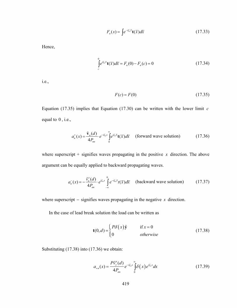
419
( ) ( )ni xnF x e x dxξ−= ∫ t (17.33)
Hence,
0
( ) (0) ( ) 0ni xn n
c
e x dx F F cξ = − =∫ t (17.34)
i.e.,
( ) (0)F c F= (17.35)
Equation (17.35) implies that Equation (17.30) can be written with the lower limit c
equal to 0 , i.e.,
0
( )( ) ( )4
n ni x i xnn
nn
da x e e x dxP
ξ ξ∞
−+ = ⋅ ∫v t% (forward wave solution) (17.36)
where superscript + signifies waves propagating in the positive x direction. The above
argument can be equally applied to backward propagating waves.
0( )( ) ( )
4n n
xi x i xn
nnn
v da x e e t x dxP
ξ ξ−−
−∞
= − ⋅ ∫% (backward wave solution) (17.37)
where superscript − signifies waves propagating in the negative x direction.
In the case of lead break solution the load can be written as
( ) ˆ if 0
(0, )0 P x x
dotherwise
δ =⎧⎪= ⎨⎪⎩
yt (17.38)
Substituting (17.38) into (17.36) we obtain:
( )0
( )( )
4n n
ny i x i x
nnn
Pv da x e x e dx
Pξ ξδ
∞−
+ = ∫%
(17.39)

420
The integral in the wave field amplitude (17.39) is the Fourier integral of the Dirac delta
function; it can be solved and it is equal to one. Hence, Equation (17.39) becomes
( )
( )4
ni xny
nnn
v d ea x P
P
ξ−+ =
% (17.40)
From Equation (17.40) we derive the expression of the particle displacement, i.e.,
( )( )
( , , ) ( ) ( ) ( )4
ni x tny
nn nn
v d ex y t a x y P y
P
ξ ω− −+= =∑u u u
% (17.41)
Theoretical predictions and experimental results should be compared to validate the
theory developed.

421
18 CONCLUSIONS AND FUTURE WORK
This dissertation has addressed the fundamental studies in the Lamb-wave interaction
between piezoelectric wafer active sensor (PWAS) and host structure during structural
health monitoring (SHM.). The application of PWAS-based SHM for the detection of
damages in structures guided waves methods has experienced an ascending trend.
However, to achieve the large deployment of these SHM techniques and to be able to
perform in-situ and online SHM, the physics of wave excitation in the structure must be
fully understood.
The discussion in this dissertation began with the generic formulation for ultrasonic
guided waves in thin wall structures. The formulation was generic because, unlike many
authors, in many parts of our derivation (power flow, reciprocity theorem, orthogonality,
etc.) we stayed away from specifying the actual mathematical expressions of the guided
wave modes and maintained a generic formulation throughout. We also studied the power
flow and energy conservation mechanisms associated with the guided waves with
particular interest on power flow of circular crested guided waves.
The dissertation continues with the extension of the normal modes expansion (NME)
model to the case of PWAS bonded to or embedded in the structure. We developed a
theoretical prediction model of the shear transfer from PWAS to the structure through a
bond layer without limitations on the frequency and the number of modes present. We
solved the resulting integro-differential equation for shear lag transfer; we applied these

422
results to predicting the tuning between guided waves and PWAS and obtained excellent
agreement with experimental results. Another novel aspect covered in this dissertation is
that of guided waves in composite materials. The NME theory is extended to the case of
composites and we developed a generic formulation for the tuning curves that was not
directly dependent on the composite layup and could be easily extended to various
composite formulations. We conducted carefully-planned experiments on composites
with different orientations. The comparison between our predictions and experiments was
quite good.
In the last part of the dissertation, SHM issues and applications are presented. We
discussed the reliability of SHM systems and the lack of quality specifications for SHM
inspections with particular focus on the case of composites SHM. We determined
experimentally the ability of PWAS to detect damage in various composite specimens.
We tested the performance of PWAS for damage detection on composite plates, on
unidirectional composite strips, on quasi-isotropic plates, on lap-joints junctions, and
composite tank sections. We also tested the ability of PWAS transducers to operate under
extreme environments and high stress conditions, i.e. the survivability of PWAS-based
SHM. We proved the durability of the entire PWAS-based SHM system under various
different load conditions. We also tested the influence of bond degradation on PWAS
electrical capacitance as installed on the structure, which gives a measure of the quality
of the PWAS installation, a key feature in PWAS-based SHM. We developed theoretical
models for shear horizontal waves scattering from a crack and Lamb waves scattering
from change in material properties. We studied the acoustic emission (AE) in infinite
plate and we used NME to model AE phenomena.
423
A review of the main results of this dissertation is given next.
18.1 RESEARCH CONCLUSIONS
18.1.1 Elastic waves for structural health monitoring
The aim of the discussion was to provide first a generic derivation valid for guided waves
propagation in a layered media assuming an orthogonal coordinate system. First, the
theory of guided waves propagation was thoroughly studied; then, a more detail
derivation for both shear horizontal waves and Lamb waves was provided for the case of
isotropic materials considering both straight-crested and circular-crested guided waves.
The major findings are listed as follows:
(1.) Acoustic field equations independent of material of the media and orthogonal
coordinate system can be derived only in Vogit notations.
(2.) Solution of the circular-crested Lamb waves can be obtained by assuming that the
dilatation varies with the thickness as a sine and cosine function. There is no need
to assume hyperbolic functions.
(3.) From the solution of the circular shear horizontal waves, we notice that the
particle displacements and stresses distributions across the thickness are equal to
those derived for straight crested shear horizontal waves.
(4.) The particle displacements variations across the thickness are the same for both
straight-crested and circular-crested Lamb waves.
(5.) The stresses distributions across the thickness are the same for both straight-
crested and circular-crested Lamb waves, except for the normal stress in the
direction of the propagation of the wave. The circular-crested Lamb waves radial

424
stress has an additional term that becomes negligible as the distance from the
source increases.
18.1.2 Power flow and orthogonality relations
The major findings of the research on power flow and orthogonality relations are listed as
follows:
(1.) For time-harmonic guided waves, half of the real part of the complex power flow
represents the time-averaged power over a time period T.
(2.) The average power flow of a guided wave through a surface is equal to zero if
both forward and backward propagating waves are considering.
(3.) To obtain the average power flow the contribution from forward and backward
waves must be separated.
(4.) For straight-crested waves, the D’Alambert formulation of the solution provides a
straightforward way to obtain the wave separation between forward and backward
waves.
(5.) Power flow for circular crested wave is present in literature of structural guided
waves only for wave propagating in cylinders or tubes. No derivation is present in
literature for wave propagating radially.
(6.) No D’Alambert solution is possible for circular crested waves. However, through
the use of the complex form of the solution of circular-crested waves, we were
able to separate the inward propagating wave from the outward propagating wave
and obtain the average power flow.

425
(7.) Real and complex reciprocity relations can be derived without the need to specify
the material of the medium or the orthogonal coordinate system.
(8.) Guided waves form a complete set of orthogonal functions. If the wave is a
propagating wave (i.e., real wavenumber), the power flow is carried by the cross-
product of the propagating mode with itself. If the wave is an evanescent wave
(i.e., imaginary wavenumber), the power flow is carried by the cross product of
the positive evanescent mode and its reflected mode (negative wavenumber).
(9.) For straight-crested waves is possible to prove the orthogonality of the guided
wave functions without specifying the particular solution. This is not possible for
circular-crested waves.
(10.) The normalization factor is the same in any coordinate system.
18.1.3 Excitation of guided waves and shear layer coupling between PWAS and
structure
The major findings of the research on excitation of guided waves and shear layer
coupling between PWAS and structure are listed as follows:
(1.) PWAS bonded on an isotropic plate can only excite Lamb waves.
(2.) The NME theory has been extended to circular crested waves.
(3.) NME is a useful method to study guided wave excited by one or two PWAS
installed on the surface of a structure or embedded in a structure.
(4.) The shear-lag model is provided for any frequency and number of wave modes
present through the use of NME theory.

426
(5.) There is difference at low frequency between the shear-lag derivation without
assumptions and the shear-lag derived with the low frequency approximation. The
difference is due to the Euler-Bernoulli assumption made in the latter.
(6.) The influence of the different parameters of the PWAS-bond-system on the shear
transfer distribution is discussed in detail.
(7.) The importance of the evanescent modes in the derivation of the shear-lag is
reported in detail.
18.1.4 Tuned guided waves in structures
The major findings of the research on tuned guided waves in structures are listed as
follows:
(1.) Forcing functions for ideal bond conditions, shear-lag parameter with low
frequencies approximation, and shear-lag for N generic modes are derived and
compared.
(2.) Tuning curves are derived through the NME method. The formulation gives the
same results as the integral Fourier derivation. This is shown numerically and
analytically.
(3.) Experimental data and theoretical predictions are compared for various PWAS
geometry and plate thickness. There is agreement between predictions and
experiments.
(4.) Tuning curves predictions through ideal bond assumptions need a correction
factor in the PWAS length. However, the correction factor is not needed when the
shear-lag model is used.

427
(5.) Theoretical tuning curves are developed for composite plates.
(6.) The tuning curve formulation does not depend on the particular method used to
extract the dispersion curves of the guided waves propagating in the composite
plate.
(7.) A program to extract dispersion and group velocities curves in composite plates of
layered materials is available.
(8.) Predictions and experimental data for quasi-antisymmetric wave propagating in a
quasi-isotropic plate made of 16 layers are compared. The data are in good
agreement.
18.1.5 Reliability of SHM
The major findings of the research on reliability of SHM are listed as follows:
(1.) Specifications for the reliability of quality SHM inspections are not available.
(2.) SHM relies on the specifications derived for NDE systems; however, these are not
always valid for SHM systems.
(3.) Probability of detection (POD) curves have not been derived for any SHM
system. The major problem is that POD curves for SHM are influenced by many
factors. To obtain POD curves, several experiments for each factor should be
considered. Cost and time limitations have been the major drawbacks.
18.1.6 Space-qualified SHM
(1.) PWAS are able to perform damage detection at cryogenic temperatures.
(2.) Electro mechanical impedance does not change with thermal fatigue.

428
(3.) PWAS are able to detect damage due to holes, impact, and delamination in
composite structures of different thickness, layer lay-up, and geometry.
(4.) SHM using PWAS is a space-qualified system for damage detection.
18.1.7 Survivability and durability of SHM systems
(1.) SHM systems with PWAS can survive extreme low temperatures and stress
conditions and still be operative.
(2.) The weak points in the PWAS-based SHM system are the solder between PWAS
and electric wire and the bond layer between PWAS and structure.
(3.) Through the combined use of E/M impedance and wave propagation it is possible
to asses the functionality o f the SHM system and the health of the structure.
(4.) SHM using PWAS can withstand space qualification tests and pass the lunch
requirement for the system.
(5.) Ranges of capacitance of the PWAS bonded on an aluminum structure are given
for good bond, partial bond, and non-bonded PWAS. These ranges can be used as
a reference for the operator.
18.1.8 Scattering from a crack and acoustic emission detection
(1.) Theoretical formulation of Lamb wave scattering is not possible without the use
of finite element models.
(2.) A simple derivation for scattering from a partial crack is derived for SH waves.
(3.) The generic problem for Lamb waves scattering from material inhomogeneity and
thickness change is provided.
429
(4.) A review of the available AE modeling shows that few models are applicable for
PWAS AE detection.
(5.) An integral Fourier formulation is derived for modeling the in-plane particle
displacement due to an AE.
(6.) An alternative formulation is derived through NME theory.
18.2 MAJOR CONTRIBUTIONS
This dissertation has brought major contributions to the fundamental studies in the Lamb-
wave interaction between PWAS and host structure during SHM. Some of these are novel
and had not been found in the specialized literature. Hereunder, we report a list of the five
most important contributions.
(1.) Development of the shear-lag solution for N generic guided wave modes present.
(2.) Extension of the derivation of tuning curves to anisotropic materials through
NME. (For the first time)
(3.) Derivation of orthogonality relations without specific mathematical expressions.
(For the first time)
(4.) Application of statistical models to damage identification algorithms
(5.) Demonstration through experiments that PWAS-based SHM can be applied to
composites in extreme environments towards space qualification.

430
18.3 RECOMMENDATION FOR FUTURE WORK
The research presented in this dissertation can be used in the development of an efficient
PWAS-based SHM system. The following tasks are recommended to be undertaken to
continue the research:
(1.) Extend the shear-lag solution to the circular crested guided waves.
(2.) Extend the shear-lag solution to anisotropic materials.
(3.) Explore the contribution of complex wavenumbers and higher order imaginary
wave modes to the shear-lag solution.
(4.) Experimentally verify the shear-lag derived with the N generic model.
(5.) Extend the derivation of tuning curve through NME to circular crested waves and
compare with the integral Fourier derivation in 2-D.
(6.) Investigate which specifications are needed to obtain a reliable system, in
particular determine whether POD curves are needed for SHM or if alternative
methods can be found.
(7.) A more reliable connection between PWAS and electric wire and bond between
PWAS and structure should be explored.
(8.) Capacitance interval of the good bond of PWAS on different materials should be
provided and used to determine the quality of the bond.
(9.) Scattering models with finite elements methods should be implemented. These
can be useful to determine the best PWAS lay out for damage detection in a
structure.

431
(10.) The AE model through integral Fourier method and NME method should be
verified against experimental data.

432
19 REFERENCES
ASM Handbook, (1992) “Nondestructive Evaluation and Quality Control”, ASM International,
Materials Park, Ohio, Vol. 17
Alleyne D. N., Cawley P., (1992) “The interaction of Lamb waves with defects”, IEEE
Transactions on Ultrasonics, Ferroelectrics, and Frequency Control, Vol. 39, No. 3,
May, 1992
Auld B. A. (1990) “Acoustic Fields and waves in solids”, John Wiley & Son Vol. 1 and 2, 1990
Bao J., 2003 “Lamb wave generation and detection with piezoelectric wafer active sensors”,
Dissertation, University of South Carolina, 2003.
Chambers J. T. , Wardle B. L., Kessler S. S. (2006) “Durability Assessment of Lamb Wave-
Based Structural Health Monitoring Nodes”, Proceedings of the 47th
AIAA/ASME/ASCE/AHS/ASC Structures, Structural Dynamics, and Materials
Conference. 1–12. May 2006.
Cho Y., (2000) “Estimation of ultrasonic guided wave mode conversion in a plate with thickness
variation”, IEEE Transaction on Ultrasonics, Ferroelectrics, and Frequency Control,
Vol. 47, No. 3, May, 2000
Cho Y., Rose J. L., (1996) “A boundary element solution for a mode conversion study on the
edge reflection of Lamb waves”, Journal of Acoustic Society of American, April, 1996
Courant, R.; Hilbert, D. (1953) “Methods of mathematical physics”, Vol I, Interscience, New
York, 1953

433
Crawley, E. F.; de Luis, J. (1987) “Use of Piezoelectric Actuators as Elements of Intelligent
Structures”, AIAA Journal, Vol. 25, No. 10, pp. 1373-1385, 1987
Crawley, E. F.; Anderson, E. H. (1990) “Detailed Models of Piezoceramic Actuation of Beams”,
Journal of Intelligent Material Systems and Structures, Vol. 1, No. 1, Jan. 1990, pp. 4-
25De Hoop, A. T. (1988) “Time domain reciprocity theorems for acoustic wave fields in
fluids with relaxation” J.A.S.A., Vol. 84, p 1877-1882, 1988
Cuc A., Tidwell Z., Giurgiutiu, V., and Joshi S. (2005) “Non-Destructive Evaluation (Nde) Of
Space Application Panels Using Piezoelectric Wafer Active Sensors,” Proceedings of
IMECE2005, 5-11 Nov., paper# IMECE2005-81721
Ditri, J. J. (1996) “Some results on the scattering of guided elastic SH waves from material and
geometric waveguide discontinuities”, Journal of Acoustic Society of America, 100, 5,
1996.
Dugnani, R. (2009) “Dynamic Behavior of Structure-Mounted Disk-Shape Piezoelectric Sensors
Including the Adhesive Layer”, Journal of Intelligent Material Systems and Structures,
2009
Gakenheimer D.C.; Miklowitz J., (1969) Transient excitation of an elastic half-space by a point
load travelling on the surface, Journal of Applied Mechanics 36, 1969, pp. 505–515
Gallagher J. P., Giessler F. J., Berens A. P., (1984) “USAF Damage Tolerant Design Handbook:
Guidelines for the Analysis and Design of Damage Tolerant Aircraft Structures. Revision
B“ Dayton University OH Research institute, May 1984.
Gatti, G. G.; Harwell, M. (1998) “Advantages of Computer Programs Over Power Charts for the
Estimation of Power”, Journal of Statistics Education v.6, n.3, 1998
Giurgiutiu, V. (2008) Structural Health Monitoring with Piezoelectric Wafer Active Sensors,
Elsevier Academic Press, 760 pages, ISBN 978-0120887606, 2008

434
Giurgiutiu, V. (2005) “Tuned Lamb-Wave Excitation and Detection with Piezoelectric Wafer
Active Sensors for Structural Health Monitoring”, Journal of Intelligent Material Systems
and Structures, Vol. 16, No. 4, pp. 291-306, 2005
Giurgiutiu, V. “Structural Monitoring with Piezoelectric Wafer Active Sensors”, Final Report
#USC-ME-LAMSS-2003-101, presented to AFRL NDE Branch, contract TOPS-DO-
033-USC, July 2004
Giurgiutiu, V. (2003) “Lamb Wave Generation with Piezoelectric Wafer Active Sensors for
Structural Health Monitoring”, SPIE's 10th Annual International Symposium on Smart
Structures and Materials and 8th Annual International Symposium on NDE for Health
Monitoring and Diagnostics, 2-6 March 2003, San Diego, CA, paper # 5056-17
Giurgiutiu, V.; Harries, K.; Petrou, M.; Bost, J.; Quattlebaum, J. B. 2003, “Disbond detection
with piezoelectric wafer active sensors in RC structures strengthened with FRP
composite overlays,” Earthquake Engineering and Engineering Vibration, Vol. 2, No. 2.
Giurgiutiu, V.; Lin, B. “Durability and Survivability of Piezoelectric Wafer Active Sensors for
Structural Health Monitoring using the Electromechanical Impedance Technique”,
Proceedings of the 2004 ASME International Mechanical Engineering Congress,
November 13-19, 2004, Anaheim, CA, paper # IMECE2004-60974.
Giurgiutiu, V.; Zagrai, A. N. 2001, “Embedded self-sensing piezoelectric active sensors for
online structural identification,” ASME Journal of Vibration and Acoustics, 124:116-125.
Goodman, L. E. 1952 “Circular-crested vibrations of an elastic solid bounded by two parallel
planes”, Proceedings of the 1st National Congress of Applied Mechanics, 1952
Gorman, M. R.; Prosser, W. H., (1991) “AE source orientation by plate wave analysis”, Journal
of Acoustic Emission, Vol. 9(4), pp. 283-288, 1991

435
Gorman, M. R.; Prosser, W. H. (1990) “Application of normal mode expansion to AE waves in
finite plates”, Transactions of the ASME: Journal of Applied Mechanics, 1990
Graff K. F. (1991) “Wave motion in elastic solids”, Dover Publications, inc, New York, 1991
Grahn T., (2002) “Lamb wave scattering from a circular partly through-thickness hole in a plate”
Wave Motion, 2002
Grills, R. (2001) “Probability of Detection – An NDT Solution”, The American Society for
Nondestructive Testing, 2001
Gunawan A., Hirose S., (2004) “Mode-Exciting method for Lamb wave-scattering analysis”,
Journal of Acoustic Society of American, 115 (3), March, 2004
Hall, S. R., 1999 “The effective management and use of structural health data”, Proceedings of
the 2nd International workshop on Structural Health Monitoring, Stanford, CA, 265—275,
September 8-10, 1999
Haskell, N. A. (1953) “Dispersion of surface waves on multilayered media,” Bull. Seism. Soc.
Am., vol. 43, pp. 17–34, 1953
He J. H. (2007) “Variational iteration method—Some recent results and new interpretations”,
Journal of computational and applied mathematics, 207, 3-17, 2007
Herakovich C. T. (1998) “Mechanics of Fibrous Composites”, John Wiley & Sons, Inc 1998
Hildebrand F. B. (1964) “Advanced calculus for applications”, Prentice-Hall, Inc., Englewood
Cliffs, NJ
Hinders M. K., (1996) “Lamb waves scattering from rivets”, Quantitative nondestructive
Evaluation, Vol. 15 1996
Hsu, N. N. (1985) “Dynamic Green’s Functions of an Infinite Plate - A Computer Program,”
NBSIR 85-3234, 1985

436
Ihn, J.-B.; Chang, F.-K. (2008) “Pitch-catch Active Sensing Methods in Structural Health
Monitoring for Aircraft Structures”, Structural Health Monitoring – An International
Journal, Vol. 7, No. 1, pp. 5-19
Kausel E., (1986) “Wave propagation in anisotropic layered media” International Journal for
Numerical Methods in Engineering, Vol. 23, 1567-1578, 1986
McKeon J. C. P., Hinders M. K., (1999) “Lamb waves scattering from a through hole”, Journal of
Sound and Vibration,224(5), 843-862, 1999
Kessler, S.S., (2005) “Certifying a Structural Health Monitoring System: Characterizing
Durability, Reliability and Longevity,”, Proceedings of the 1st International Forum on
Integrated Systems Health Engineering and Management in Aerospace, Napa, CA, 7-10
November 2005.
Kessler S. S., Spearing M. S., Soutis C., (2001) “Damage detection in composite materials using
Lamb wave methods”, Smart Materials and Structures, August, 2001
Lin, B.; Giurgiutiu, V.; Pollock, P.; Xu, B.; Doane, J.; (2009) “Durability and Survivability of
Piezoelectric Wafer Active Sensors on Metallic Structure”, AIAA Journal , (Accepted)
Liu, L.; Yuan, F.-G. (2008) ”Active damage localization for plate-like structures using wireless
sensors and a distributed algorithm”, Smart Materials And Structures, Vol. 17 (2008)
#055022 (on line)
Lu, Y.; Michaels, J. E. (2008) “Numerical Implementation of Matching Pursuit for the Analysis
of Complex Ultrasonic Signals”, IEEE Transactions on Ultrasonics, Ferroelectronics,
and Frequency Control, Vol.55, No.1, pp.173-182
Lowe M. J. S., (1995) “Matrix technique for modeling ultrasonic waves in multilayered media”
IEEE, July, 1995

437
Lowe M. J. S., Diligent O. (2002) “Low-frequency reflection characteristics of the s0 Lamb wave
from a rectangular notch in a plate”, Journal of Acoustic Society of America, January
2002
Luo, Q.; Tong, L. (2002), “Exact static solutions to piezoelectric smart beams including peel
stresses”, International Journal of Solids and Structures, Vol. 39, 2002, pp. 4677–4722
Masserey B., Mazza E. (2005) “Analysis of the near-field ultrasonic scattering at a surface
crack”, Acoustical Society of America, 3585-3594, September 2005
Matt H., Bartoli I., Lanza di Scalea F., (2005) “Ultrasonic guided wave monitoring of composite
wing skin-to-spar bonded joints in aerospace structures” Journal of Intelligent Materials,
2005
Nayfeh A. H., (1991) “The general problem of elastic wave propagation in multilayered
anisotropic media” Journal of Acoustical Society of America, 89 (4), Pt. 1, April 1991
Nayfeh A. H., (1995) “Wave propagation in layered anisotropic media with application to
composites” Elsevier, 1995
Medick, M. A. (1961) “On classical plate theory and wave propagation”, Journal of Applied
Mechanics, 1961, Vol. 28, pp 223-228
Moreau, L., Castaings, M. (2008) “The use of an orthogonality relation for reducing the size of
finite element models for 3D guided waves scattering problems”, Ultrasonics, 48, 357-
366, 2008
Morse M. P.; Feshbach H., (1953) “Methods of theoretical physics”, McGraw-Hill Book
Company, Inc., vol 1 and 2, 1953
Pao, Y. H.; Gajewski, R. R.; Ceranoglu, A. N. (1979) “Acoustic Emission and Transient Waves
in an Elastic Plate,” Journal of Acoustical Society of America, 65, 1979, pp. 96-105

438
Pao, Y. H. (1978) “Theory of Acoustic Emission,” Elastic Waves and Nondestructive Testing,
AMD-29, Am. Soc. Mech. Engr., New York, 1978, pp. 107-128
Park, S.; Park, G.; Yun, C.-B.; Farrar, C. R. (2009) “Sensor Self-diagnosis Using a Modified
Impedance Model for Active Sensing-based Structural Health Monitoring”, Structural
Health Monitoring – An International Journal, Vol. 8, No. 1, Jan. 2009, pp. 71-82
Prosser, W. H.; Hamstad, M. A.; Gary, J.; O’Gallagher, A. (1999). “Finite element and plate
theory modeling of acoustic emission waveforms”, Journal of Nondestructive Evaluation
18(3):83–90.
Prosser, W. H. (1991) “The Propagation Characteristics of the Plate Modes of Acoustic Emission
Waves in Thin Aluminum Plates and Thin Graphite/Epoxy Composite Plates and Tubes”,
NASA Technical Memorandum 104187, November, 1991
Pursey, H., (1957) “The Launching and propagation of elastic waves in plates”, Quarterly journal
of mechanics and applied mathematics, 10, pp. 45-62, 1957
Raghavan A., Cesnik C. E. S., (2005) “Piezoelectric-actuator excited-wave field solutions for
guided-wave structural health monitoring”, Smart Structures and Materials 2005: Sensors
and Smart Structures Technologies for Civil, Mechanical, and Aerospace Systems,
Masayoshi Tomizuka, Editors, pp.313-323
Raghavan A., Cesnik C. E. S. (2004) "Modeling of piezoelectric-based Lamb-wave generation
and sensing for structural health monitoring"; Proceedings of SPIE - Volume 5391 Smart
Structures and Materials 2004: Sensors and Smart Structures Technologies for Civil,
Mechanical, and Aerospace Systems, Shih-Chi Liu, Editor, July 2004, pp. 419-430
Rokhlin S. I., Wang L., (2002) “Stable recursive algorithm for elastic wave propagation in
layered anisotropic media: Stiffness matrix method”, Journal of Acoustic Society of
America, June, 2002

439
Rose J. L. (1999) “Ultrasonic waves in layered media”, Cambridge University Press, 1999
Ryu D. H.; Wang K. W. (2004) “Analysis of interfacial stress and actuation authorities induced
by surface-bonded piezoelectric actuators on curved flexible beams”, Smart Materials
and Structures, Vol. 13, No. 4, August 2004, pp. 753-761
Tang B., Henneke E. G. II, (1989) “Long wavelength approximation for Lamb wave
characterization of composite laminates”, Research in Nondestructive Evaluation, Vol. 1,
Issue 1, Mar 1989, Pages 51 - 64, 1989
Thomson, W. T. (1950) “Transmission of elastic waves through a stratified solid medium,” J.
Appl. Phys., vol. 21, pp. 89–93, 1950
Tong, L.; Luo, Q. (2003) “Exact dynamic solutions to piezoelectric smart beams including peel
stresses”, International Journal of Solids and Structures, Vol. 40, 2003, pp. 4789–4836
Vemula C., Norris A. N., (2005) “Flexural wave propagation and scattering on thin plates using
Mindlin theory” Wave Motion, 26, I-12, June, 2005
Viktorov, I. A. (1967) Rayleigh and Lamb Waves – Physical Theory and Applications, Plenum
Press, NY,1967
Wang L., Rokhlin S. I., (2001) “Stable reformulation of transfer matrix method for wave
propagation in layered anisotropic media”, Ultrasonics, 39 (2001), 413-424
Wang S. Q., He J. H. (2007), “Variational iteration method for solving integro-differential
equations”, Physics Letters A, 367, 188-191, 2007
Xi L. (2002) “Elastic waves in anisotropic laminates”, CRC Press, 2002
Zhongqing S., Ye, L., (2005)“Lamb wave propagation-based damage identification for quasi-
isotropic CF/EP composite laminates using artificial neural algorithm: Part II -

440
Implementation and validation” Journal of Intelligent Material Systems and Structures,
Vol. 16, 2005.
Zill D. G., Cullen M. R. (2001) “Differential Equations with Boundary-Value Problems”,
Brooks/Cole 5th ed.

441
APPENDIX

442
A EQUATION OF MOTION IN CYLINDRICAL COORDINATES In the first section of the appendix we will show the general formulation for the equation
of motion as described in continuum mechanics. In the second part of the appendix we
will derive the equation of motion in cylindrical coordinates from equilibrium
considerations.
A.1 EQUATIONS OF MOTION IN CONTINUUM MECHANICS The equations of motion in continuum mechanics are derived from the conservation of
linear momentum. Consider a region R in space where exists a material volume of density
ρ having surface tractions and body forces acting upon it. Denote with iu the
displacement of the material volume. The second law of Newton states that the rate of
change of linear momentum equals the resultant force on the volume. The change in
linear momentum can be expressed as
2
2 iRu d
tρ τ∂
∂ ∫∫∫ (A.1)
where dτ is an element of volume and ρ is the material density per unit volume. The
force applied to the volume is equal to
jij iS Rn dS f dσ ρ τ+∫∫ ∫∫∫ (A.2)
where ijσ are the contravartiant components of the stress tensor, jn is the normal to the
surface S, dS is an element of the surface area, jf are the body forces per unit mass.

443
Note that ( )j nij in tσ = are the component of the surface traction forces ( )nt
r associated with
the plane with normal n. Combining Equations (A.1) and (A.2), Newton’s second law
becomes
2
2j
i ij iR S Ru d n dS f d
tρ τ σ ρ τ∂
= +∂ ∫∫∫ ∫∫ ∫∫∫ (A.3)
Recall the Gauss divergence theorem, i.e.,
,j
i j iV SF d F n dSτ =∫∫∫ ∫∫ (A.4)
Use Equation (A.4) in Equation (A.3) to obtain
2
,2 i ij j iR R Ru d d f d
tρ τ σ τ ρ τ∂
= +∂ ∫∫∫ ∫∫∫ ∫∫∫ (A.5)
Rearrange the terms and note that the time derivative can be brought inside the volume
integral, hence we get
2
,2 0iij j iR
u f dt
ρ σ ρ τ⎛ ⎞∂
− − =⎜ ⎟∂⎝ ⎠∫∫∫ (A.6)
Since the integral must be true for any given region R of the volume, Equation (A.6)
implies
2
,2 0iij j i
u ft
ρ σ ρ∂− − =
∂ (A.7)
and in absence of external forces, Equation (A.7) simplifies as
2
, 2 0iij j
ut
σ ρ ∂− =
∂ (A.8)

444
The derivate if the contravariant components of the stress tensor can be expressed as (see
Heibockel)
[ ], 2 2 2 2
1 ,ij mjij j iij
i j m jii
g g ij mx h h h hg g
σ σσ
⎛ ⎞∂= −⎜ ⎟∂ ⎝ ⎠
(A.9)
where ijg are the metric components of the coordinate system considered, i iih g= , and
the second term in Equation (A.9) can be expressed as
[ ]2
2 2 2 2 2 2
1 1,2 2
mj mj jm ij jj jimj i m i
m j m j j j
g g hgij mh h h h x x x h h xσ σ σ∂ ∂ ∂⎛ ⎞∂
= + + =⎜ ⎟∂ ∂ ∂ ∂⎝ ⎠ (A.10)
Hence, the stress tensor derivate is equal to
2
, 2 2 2 2
1 12
ij jj jij j iij i
i j j jii
hg g
x h h h h xg gσ σ
σ∂⎛ ⎞∂
= −⎜ ⎟∂ ∂⎝ ⎠ (A.11)
In order to express Equation (A.11) in terms of physical components in orthogonal
systems, we must perform the following transformation
( )
( )ij i j
ii
ii
ij h h
b i hbg
σ σ=
= (A.12)
Using (A.12), Equation (A.11) becomes
23 3
, 21 1
1 1 ( ) 1 ( )2
jij j iij i
j jii i j j
hij jjg gg x h h h xg
σ σσ= =
∂∂ ⎛ ⎞= −⎜ ⎟∂ ∂⎝ ⎠∑ ∑ (A.13)
Substitute Equation (A.13) into the equation of motion (A.7) to obtain
2 23 3
2 21 1
1 1 ( ) 1 ( ) ( ) 02
j iiij i
j jii i j j ii
h hij jj u ig gg x h h h x g tg
σ σ ρ= =
∂∂ ∂⎛ ⎞ − − =⎜ ⎟∂ ∂ ∂⎝ ⎠∑ ∑ (A.14)

445
Equation (A.14) is the equation of motion in any orthogonal coordinate system. Recall
that for any orthogonal system it is 0ijg = for i j≠ . Expand the equation of motion to
get a system of three equations, i.e.,
2 23 31
11 2 1 21 111 1 11
2 23 32
22 2 2 21 122 2 22
23
33 21 33 3
1 1 ( ) 1 ( ) ( ) 02
1 1 ( ) 1 ( ) ( ) 02
1 1 ( ) 1 ( )2
jj
j jj j
jj
j jj j
jj
j j j
h hij jj u ig gg x h h h x g tg
h hij jj u ig gg x h h h x g tg
hij jjg gg x h h hg
σ σ ρ
σ σ ρ
σ σ
= =
= =
=
∂∂ ∂⎛ ⎞ − − =⎜ ⎟∂ ∂ ∂⎝ ⎠∂∂ ∂⎛ ⎞ − − =⎜ ⎟∂ ∂ ∂⎝ ⎠∂∂ ⎛ ⎞ −⎜ ⎟∂ ∂⎝ ⎠
∑ ∑
∑ ∑
∑23
33 2
1 33
(3) 0j
h ux g t
ρ=
⎧⎪⎪⎪⎪⎨⎪⎪
∂⎪ − =⎪ ∂⎩
∑
(A.15)
In Cartesian coordinates we have that
11 22 33
1 2 3
11 22 33
11
1
g g gh h hg g g g
= = =⎧⎪ = = =⎨⎪ = =⎩
(A.16)
With the use of relations in Equation (A.16), the equations of motion (A.15) become
2
2
2
21 2 3
2
21 2 3
0
0
0
xyxx xz x
xy yy yz y
yzxz zz z
ux y z t
ux x x t
ux x x t
σσ σ ρ
σ σ σρ
σσ σ ρ
∂⎧∂ ∂ ∂+ + − =⎪ ∂ ∂ ∂ ∂⎪
⎪∂ ∂ ∂ ∂⎪ + + − =⎨∂ ∂ ∂ ∂⎪
⎪ ∂∂ ∂ ∂⎪ + + − =∂ ∂ ∂ ∂⎪⎩
(A.17)
In cylindrical coordinates we have that
11 33 1 3
222 2
211 22 33
1g g h h
g h r
g g g g r
= = = =⎧⎪
= =⎨⎪ = =⎩
(A.18)
With the use of relations in Equation (A.16), the equations of motion (A.15) become

446
2
2
2
2
2
2
1 0
1 2 0
1 0
r rr irr rz
r z r
zrz zz rz z
ur r r r t
ur r z r t
ur r z r t
θ θθ
θ θθ θ θ θ
θ
σ σ σσ σ ρθ
σ σ σ σ ρθ
σσ σ σ ρθ
∂ − ∂∂ ∂+ + + − =
∂ ∂ ∂ ∂∂ ∂ ∂ ∂
+ + + − =∂ ∂ ∂ ∂
∂∂ ∂ ∂+ + + − =
∂ ∂ ∂ ∂
(A.19)
In spherical coordinates we have that
211 1
2 222 2
2 2 233 3
4 211 22 33
1
sin
sin
g h
g h
g h
g g g g
ρ
ρ θ
ρ θ
⎧ = =⎪
= =⎪⎨
= =⎪⎪ = =⎩
(A.20)
With the use of relations in Equation (A.16), the equations of motion (A.15) become
( )
2
3 2
2
3 2
2
1 1 1 cos 2 0sin sin
1 1 1 cos3 0sin sin
1 1 1 cos3 2sin sin
rux t
ux t
ρρ ρθ ρφρθ ρρ θθ φφ
ρθ θφθθ θρθ θθ φφ
ρφ θφ φφρφ θφ
σ σ σ θ σ σ σ σ ηρ ρ θ ρ θ ρ θ
σ σσ θσ σ σ ηρ ρ θ ρ θ ρ θ
σ σ σ θσ σ ρρ ρ θ ρ θ φ ρ θ
∂ ∂ ∂ ∂⎛ ⎞+ + + + − − − =⎜ ⎟∂ ∂ ∂ ∂⎝ ⎠∂ ∂∂ ∂⎡ ⎤+ + + + − − =⎢ ⎥∂ ∂ ∂ ∂⎣ ⎦∂ ∂ ∂ ∂⎛ ⎞+ + + + −⎜ ⎟∂ ∂ ∂ ⎝ ⎠ 2
(3) 0ut
⎧⎪⎪⎪⎪⎨⎪⎪
=⎪∂⎪⎩
(A.21)
A.2 EQUATIONS OF MOTION FROM EQUILIBRIUM CONSIDERATION Consider a plate in a cylindrical coordinate system. The distance r of a point P of the
plate from the origin O is defined by the angle θ between r and an axis Ox fixed in the
plate (Figure A.1). The distance OP is equal to r.
Consider the equilibrium of the volume element in the radial direction. The normal
stress ( )1rσ acts on the surface 1r d dzθ , where 1r is the radium of the side 1. Hence the
force on surface 1 along the radium is equal to
( ) 11r r d dzσ θ (A.22)

447
Figure A.1 Equilibrium of a small element of a plate.
Similarly, the radial force on surface 3 is given by
( ) 33r r d dzσ θ− (A.23)
The component of the normal force ( )2θσ on surface 2 along the radii gives a negative
contribute to the net force, i.e.,
( )2sin
2ddrdzθθσ− (A.24)
The component of the normal force ( )4θσ on surface 4 along the radii gives a negative
contribute to the net force, i.e.,
( )4sin
2ddrdzθθσ− (A.25)
The shear stress ( )2rθτ on surface 2 and the shear stress ( )4rθτ on surface 4 give a net
contribution given by
( ) ( )2 4r r drdzθ θτ τ⎡ ⎤−⎣ ⎦ (A.26)
x
z
O
P 1
2
3 4
5
6
dθ θ
y
x
y
O
P
2
3 4
dθθ
1
(σr)1
(σr)3
(σθ)4
(σθ)2
(τrθ)4
(τrθ)2(τrθ)1
(τrθ)3
(τθz)5(τθz)2(τrz)5
(τrz)1
(σz)5
(τθz)4
(τrz)3
5

448
The shear stress ( )5rzτ on surfaces 5 and the shear stress ( )6rzτ on surface 6 give a net
contribution given by
( ) ( )5 6rz rz rd drτ τ θ⎡ ⎤−⎣ ⎦ (A.27)
Sum all the forces along the radial direction and add the body forces contribution R to
obtain
( ) ( ) ( ) ( ) ( ) ( )
( ) ( )
1 31 3 2 4 2 4
5 6
sin2 2
0
r r r r
rz rz
d dr r d dz drdz drdz
drd Rrd drdz
θ θ θ θθ θσ σ θ σ σ τ τ
τ τ θ θ
⎡ ⎤⎡ ⎤ ⎡ ⎤− − − + −⎢ ⎥⎣ ⎦ ⎣ ⎦⎣ ⎦⎡ ⎤+ − + =⎣ ⎦
(A.28)
Divide Equation (A.28) by the volume drd dzθ to get
( ) ( ) ( ) ( )
( ) ( ) ( ) ( )
1 31 3 2 4
5 62 4
sin sin2 2
0
r r
r r rz rz
r r d ddr d d
r Rrd dz
θ θ
θ θ
σ σ σ σθ θθ θ
τ τ τ τθ
−− − +
− −+ + + =
(A.29)
Note that Equation (A.29) can be alternatively written as
( ) ( ) ( ) ( ) ( ) ( ) ( ) ( )1 3 5 62 4 2 4 0
2r r r r rz rzr r
r Rrdr d dz
θ θ θ θσ σ σ σ τ τ τ τθ
− + − −− + + + = (A.30)
As the dimensions of the element get smaller, the terms in Equation (A.30) can be
approximated as after rearrangement
1 0r rr rz Rr r z r
θ θτ σ σσ τθ
∂ −∂ ∂+ + + + =
∂ ∂ ∂ (A.31)
Consider now the equilibrium of the volume element in the angular direction. We have
the following contributions: Normal force on surface 2

449
( )2drdzθσ (A.32)
Normal force on surface 4
( )4drdzθσ− (A.33)
Contribution from the shear forces on surfaces 1 and 3
( ) ( )1 31 3r rr r d dzθ θτ τ θ⎡ ⎤−⎣ ⎦ (A.34)
Contribution from the shear forces on surfaces 2 and 4
( ) ( )2 4sin
2r rddrdzθ θθτ τ⎡ ⎤+⎣ ⎦ (A.35)
Contribution from the shear forces on surfaces 5 and 6
( ) ( )5 6z z rd drθ θτ τ θ⎡ ⎤−⎣ ⎦ (A.36)
The total force in the angular direction plus the component of the body force S per unit
volume divided by the element volume gives
( ) ( ) ( ) ( ) ( ) ( ) ( ) ( )1 31 3 5 62 4 2 4 0
2r r z zr rr r
r Srd dr dz
θ θ θ θθ θ θ θτ τ τ τσ σ τ τθ
− −− ++ + + + = (A.37)
As the dimensions of the element get smaller, the terms in Equation (A.37) can be
approximated as after rearrangement
1 2 0r r z Sr r r z
θ θ θ θτ σ τ τθ
∂ ∂ ∂+ + + + =
∂ ∂ ∂ (A.38)
The equilibrium of the volume element in the z direction is given by the following
contributions: Normal force on surface 5

450
( )5z drrdσ θ (A.39)
Normal force on surface 6
( )6z drrdσ θ− (A.40)
Contribution from the shear forces on surfaces 1 and 3
( ) ( )1 31 3rz rzr r d dzτ τ θ⎡ ⎤−⎣ ⎦ (A.41)
Contribution from the shear forces on surfaces 2 and 4
( ) ( )2 4z z drdzθ θτ τ⎡ ⎤−⎣ ⎦ (A.42)
The total force in the z direction plus the component of the body force Z per unit volume
divided by the element volume gives
( ) ( ) ( ) ( ) ( ) ( )1 35 6 1 3 2 4 0z z rz rz z zr r
r Zrdz dr d
θ θσ σ τ τ τ τθ
− − −+ + + = (A.43)
As the dimensions of the element get smaller, the terms in Equation (A.43) can be
approximated as
0zz rzrr Zrz r
θτσ τθ
∂∂ ∂+ + + =
∂ ∂ ∂ (A.44)
or
1 0zrz z rz Zr r z r
θττ σ τθ
∂∂ ∂+ + + + =
∂ ∂ ∂ (A.45)
Equations (A.31), (A.38), and (A.45) are the equation of motion of mass subjected to
body forces expressed in cylindrical coordinates.

451
B MATHEMATIC CONCEPTS
B.1 DEL OPERATOR NOTATION FOR VOGIT MATRIX FORMALISM The Vogit notation is a transformation of the vector notation. The order of the tensor is
reduced by one in the transformation, such as a first order tensor becomes a vector and a
second order tensor becomes a first order tensor. The transformation is done by following
the rule
1 42 53 6
xx yzyy xzzz xy
→ →→ →→ →
(B.1)
Consider the first order tensor of the stresses. In vector notation the stress tensor is
defined as
xx xy xz
xy yy yz
xz yz zz
T T TT T TT T T
⎡ ⎤⎢ ⎥= ⎢ ⎥⎢ ⎥⎣ ⎦
T (B.2)
In Vogit notation Equation (B.2) becomes
1
2
3
4
5
6
xx
yy
zz
yz
xz
xy
T TT TT TT TT TT T
⎧ ⎫ ⎧ ⎫⎪ ⎪ ⎪ ⎪⎪ ⎪ ⎪ ⎪⎪ ⎪ ⎪ ⎪⎪ ⎪ ⎪ ⎪= =⎨ ⎬ ⎨ ⎬⎪ ⎪ ⎪ ⎪⎪ ⎪ ⎪ ⎪⎪ ⎪ ⎪ ⎪
⎪ ⎪⎪ ⎪ ⎩ ⎭⎩ ⎭
T (B.3)

452
Consider the second order tensor of the stiffness coefficient, i.e., ijklc=c . For
convenience we consider the case in which the stiffness tensor is symmetric. In Vogit
notation the second order tensor becomes
11 12 13 14 15 16
22 23 24 25 26
33 34 35 36
44 45 46
55 56
66
c c c c c cc c c c c
c c c cc c c
c cc
⎡ ⎤⎢ ⎥⎢ ⎥⎢ ⎥
= ⎢ ⎥⎢ ⎥⎢ ⎥⎢ ⎥⎢ ⎥⎣ ⎦
c (B.4)
B.1.1 Rectangular coordinates Divergence of a tensor A in vector notation
xyxx xz
xx yx xzyx yy yz
yx yy yz
xz yz zzzyzx zz
AA Ax y z
A A AA A A
A A Ax y z x y z
A A AAA A
x y z
∂⎧ ⎫∂ ∂+ +⎪ ⎪∂ ∂ ∂⎪ ⎪⎡ ⎤ ⎪ ⎪∂ ∂ ∂∂ ∂ ∂ ⎪ ⎪⎧ ⎫ ⎢ ⎥∇ ⋅ = = + +⎨ ⎬⎨ ⎬ ⎢ ⎥∂ ∂ ∂ ∂ ∂ ∂⎩ ⎭ ⎪ ⎪⎢ ⎥⎣ ⎦ ⎪ ⎪∂∂ ∂+ +⎪ ⎪
∂ ∂ ∂⎪ ⎪⎩ ⎭
A (B.5)
Divergence of a tensor A in Vogit notation
1 6 51
2
3 6 2 4
4
5 5 34
6
0 0 0
0 0 0
0 0 0
A A AAA x y zx z yA A A AAy z x x y zA A AA
z y x x y zA
⎧ ⎫ ⎧ ⎫⎡ ⎤ ∂ ∂∂∂ ∂ ∂+ +⎪ ⎪ ⎪ ⎪⎢ ⎥ ∂ ∂ ∂∂ ∂ ∂ ⎪ ⎪ ⎪ ⎪⎢ ⎥
⎪ ⎪ ⎪ ⎪⎢ ⎥ ∂ ∂ ∂∂ ∂ ∂ ⎪ ⎪∇ ⋅ = = + +⎨ ⎬ ⎨ ⎬⎢ ⎥∂ ∂ ∂ ∂ ∂ ∂⎪ ⎪ ⎪ ⎪⎢ ⎥⎪ ⎪ ⎪ ⎪⎢ ⎥∂ ∂ ∂ ∂ ∂∂
+ +⎪ ⎪ ⎪ ⎪⎢ ⎥∂ ∂ ∂ ∂ ∂ ∂⎪ ⎪⎣ ⎦ ⎩ ⎭⎩ ⎭
A (B.6)
Curl of a vector A in vector notation

453
yz
xx z
y
zy xx y z
AAi j k y zx A
A AAy x y z z x
A A AA A Ax yz
∂⎧ ⎫∂∂⎧ ⎫ −⎪ ⎪⎪ ⎪ ∂ ∂∂ ⎪ ⎪⎧ ⎫⎪ ⎪⎪ ⎪∂ ∂∂ ∂ ∂ ∂⎪ ⎪⎪ ⎪∇× = × = = −⎨ ⎬⎨ ⎬⎨ ⎬∂ ∂ ∂ ∂ ∂ ∂⎪ ⎪⎪ ⎪⎪ ⎪ ⎩ ⎭ ⎪ ⎪∂⎪ ⎪ ∂∂ −⎪ ⎪⎪ ⎪ ∂ ∂∂⎩ ⎭ ⎩ ⎭
A (B.7)
Curl of a vector A in Vogit notation
0
0
0
yz
xx z
y
zy x
AAy zz y AA AA
z x z xA A A
y x x y
∂⎧ ⎫∂∂ ∂⎡ ⎤ −− ⎪ ⎪⎢ ⎥ ∂ ∂∂ ∂ ⎪ ⎪⎢ ⎥ ⎧ ⎫⎪ ⎪∂ ∂∂ ∂ ⎪ ⎪⎢ ⎥∇× = − = −⎨ ⎬⎨ ⎬⎢ ⎥∂ ∂ ∂ ∂⎪ ⎪⎪ ⎪⎢ ⎥ ⎩ ⎭ ⎪ ⎪∂ ∂ ∂ ∂⎢ ⎥− −⎪ ⎪⎢ ⎥∂ ∂ ∂ ∂⎣ ⎦ ⎩ ⎭
A (B.8)
Symmetric Del operator in Vogit notation
1
2
3
3 2
3 1
2 1
0 0
0 0
0 0
0
0
0
x
s y
z
AxxAyyAAzz A
A AAz y y z
A Az x x z
A Ay x x y
∂∂ ⎧ ⎫⎡ ⎤⎪ ⎪⎢ ⎥ ∂∂ ⎪ ⎪⎢ ⎥
∂∂ ⎪ ⎪⎢ ⎥⎪ ⎪⎢ ⎥ ∂∂⎪ ⎪⎢ ⎥
∂∂ ⎪ ⎪⎢ ⎥ ⎧ ⎫ ⎪ ⎪⎢ ⎥ ∂∂ ⎪ ⎪ ⎪ ⎪∇ = =⎢ ⎥ ⎨ ⎬ ⎨ ⎬∂∂ ∂ ∂⎢ ⎥ ⎪ ⎪ ⎪ ⎪+⎩ ⎭⎢ ⎥∂ ∂ ∂ ∂⎪ ⎪⎢ ⎥ ⎪ ⎪∂ ∂ ∂ ∂⎢ ⎥ ⎪ ⎪+⎢ ⎥ ⎪ ⎪∂ ∂ ∂ ∂⎢ ⎥ ⎪ ⎪∂ ∂ ∂ ∂⎢ ⎥ ⎪ ⎪+∂ ∂ ∂ ∂⎢ ⎥ ⎪ ⎪⎣ ⎦ ⎩ ⎭
A (B.9)
The symmetric Del operator is used in the strain-displacement relation, s= ∇S u , i.e.,

454
1
2
1
2 31
32
3 243
5
3 16
2 1
0 0
0 0
0 0
2 022 0
0
uxxuyyuuzz u
u uuz y y z
u uz x x z
u uy x x y
εεεεεε
∂∂ ⎧ ⎫⎡ ⎤⎪ ⎪⎢ ⎥ ∂∂ ⎪ ⎪⎢ ⎥
∂∂ ⎪ ⎪⎢ ⎥⎪ ⎪⎢ ⎥⎧ ⎫ ∂∂⎪⎢ ⎥⎪ ⎪
∂∂ ⎪⎢ ⎥⎪ ⎪ ⎧ ⎫ ⎪⎢ ⎥⎪ ⎪ ∂∂⎪ ⎪ ⎪ ⎪ ⎪= =⎢ ⎥⎨ ⎬ ⎨ ⎬ ⎨ ⎬∂∂ ∂ ∂⎢ ⎥⎪ ⎪ ⎪ ⎪ ⎪ +⎩ ⎭⎢ ⎥∂ ∂ ∂ ∂⎪ ⎪ ⎪⎢ ⎥⎪ ⎪ ⎪∂ ∂ ∂ ∂⎪ ⎪ ⎢ ⎥ ⎪⎩ ⎭ +⎢ ⎥ ⎪∂ ∂ ∂ ∂⎢ ⎥ ⎪∂ ∂ ∂ ∂⎢ ⎥ ⎪ +∂ ∂ ∂ ∂⎢ ⎥ ⎪⎣ ⎦ ⎩
⎪⎪⎪⎪
⎪⎪⎪⎪⎪⎪⎪⎪⎭
(B.10)
B.1.2 Cylindrical coordinates For the cylindrical coordinates, the vector notation is not always appropriate. For this
motive we will only present the Vogit notation.
Divergence of a tensor A in Vogit notation
( )
( )
( )
1
2
3
4
5
6
1 0 0
10 0 0
0 0 0
1 1
1 1
1 1
rrr rz
r r z
zrz zz
ArAr r r z rArAr z r r r
r Az r r r A
A ArA Ar r r r z
rA A A Ar r r r z
ArA Ar r r z
θθ θ
θ θ θθ θ
θ
θ
θ
θ
θ
θ
θ
⎧ ⎫⎡ ⎤∂ ⋅ ∂ ∂− ⎪ ⎪⎢ ⎥∂ ∂ ∂ ⎪ ⎪⎢ ⎥
⎪ ⎪∂ ∂ ∂ ⋅ ⎪ ⎪⎢ ⎥∇ ⋅ = + =⎨ ⎬⎢ ⎥∂ ∂ ∂ ⎪ ⎪⎢ ⎥⎪ ⎪∂ ∂ ∂ ⋅⎢ ⎥⎪ ⎪⎢ ⎥∂ ∂ ∂⎣ ⎦ ⎪ ⎪⎩ ⎭
∂∂ ∂⎧ − + +⎪ ∂ ∂ ∂⎪∂ ∂ ∂
= + + +⎨ ∂ ∂ ∂∂∂ ∂
+ +∂ ∂ ∂
A
⎫⎪⎪
⎪ ⎪⎬
⎪ ⎪⎪ ⎪⎪ ⎪⎩ ⎭
(B.11)
Curl of a vector A in Vogit notation
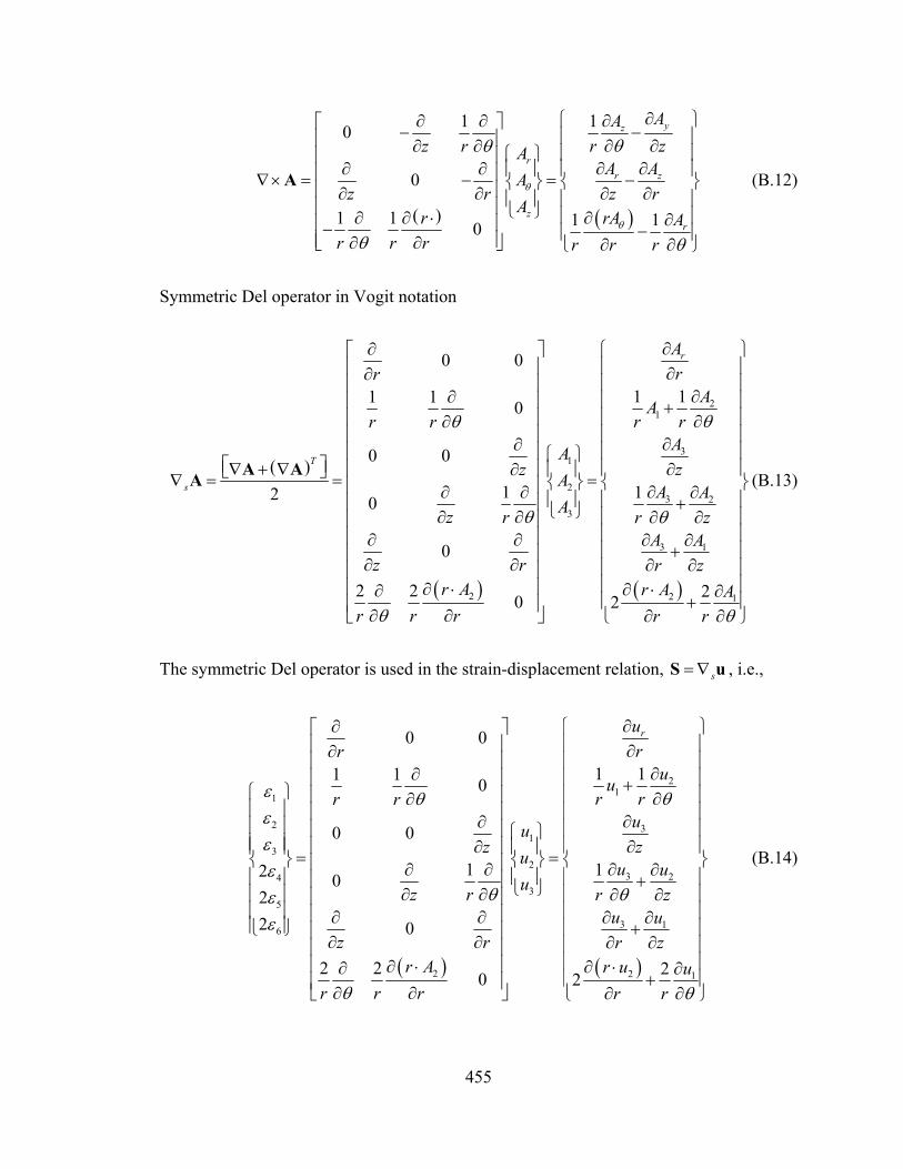
455
( ) ( )
110
0
1 1 1 10
yz
rr z
zr
AAr zz r A
A AAz r z r
Ar rA Ar r r r r r
θ
θ
θθ
θ θ
∂⎧ ⎫∂∂ ∂⎡ ⎤ −− ⎪ ⎪⎢ ⎥ ∂ ∂∂ ∂ ⎪ ⎪⎧ ⎫⎢ ⎥∂ ∂∂ ∂ ⎪ ⎪⎪ ⎪⎢ ⎥∇× = − = −⎨ ⎬⎨ ⎬⎢ ⎥∂ ∂ ∂ ∂⎪ ⎪⎪ ⎪⎢ ⎥ ⎩ ⎭ ⎪ ⎪∂ ∂ ⋅ ∂ ∂⎢ ⎥− −⎪ ⎪⎢ ⎥∂ ∂⎣ ⎦ ∂ ∂⎩ ⎭
A (B.12)
Symmetric Del operator in Vogit notation
( )
( ) ( )
21
31
23 2
3
3 1
2 2 1
0 0
1 11 1 0
0 0
1 12 0
0
2 2 20 2
r
T
s
Arr
AAr rr r
AAzz A
A AAz r r z
A Az r r z
r A r A Ar r r r r
θθ
θ θ
θ θ
∂∂ ⎧ ⎫⎡ ⎤⎪ ⎪⎢ ⎥ ∂∂ ⎪ ⎪⎢ ⎥
∂∂ ⎪ ⎪⎢ ⎥ +⎪⎢ ⎥ ∂∂⎪⎢ ⎥ ∂∂ ⎪⎢ ⎥ ⎧ ⎫⎡ ⎤ ⎪∇ + ∇ ⎢ ⎥ ∂∂ ⎪ ⎪⎣ ⎦∇ = = =⎨ ⎬ ⎨ ⎬⎢ ⎥ ∂∂ ∂ ∂⎪ ⎪ ⎪⎢ ⎥ +⎩ ⎭∂ ∂ ⎪ ∂ ∂⎢ ⎥⎪⎢ ⎥∂ ∂ ∂ ∂⎪ +⎢ ⎥∂ ∂ ∂ ∂⎪⎢ ⎥⎪⎢ ⎥∂ ⋅ ∂ ⋅∂ ∂⎪ +⎢ ⎥∂ ∂ ∂ ∂⎣ ⎦ ⎩
A AA
⎪⎪⎪⎪
⎪⎪⎪⎪⎪⎪⎪⎭
(B.13)
The symmetric Del operator is used in the strain-displacement relation, s= ∇S u , i.e.,
( ) ( )
211
2 31
32
3 243
5
3 16
2 2 1
0 0
1 11 1 0
0 0
1 12 022 0
2 2 20 2
rurr
uur rr r
uuzz u
u uuz r r z
u uz r r z
r A r u ur r r r r
ε θθεεε
θ θεε
θ θ
∂∂⎡ ⎤⎢ ⎥ ∂∂⎢ ⎥
∂∂⎢ ⎥ +⎧ ⎫ ⎢ ⎥ ∂∂⎪ ⎪ ⎢ ⎥ ∂∂⎪ ⎪ ⎢ ⎥ ⎧ ⎫⎪ ⎪ ⎢ ⎥ ∂∂⎪ ⎪ ⎪ ⎪= =⎨ ⎬ ⎨ ⎬⎢ ⎥ ∂∂ ∂ ∂⎪ ⎪ ⎪ ⎪⎢ ⎥ +⎩ ⎭∂ ∂⎪ ⎪ ∂ ∂⎢ ⎥⎪ ⎪ ⎢ ⎥∂ ∂ ∂ ∂⎪ ⎪ +⎩ ⎭ ⎢ ⎥∂ ∂ ∂ ∂⎢ ⎥
⎢ ⎥∂ ⋅ ∂ ⋅∂ ∂+⎢ ⎥∂ ∂ ∂ ∂⎣ ⎦
⎧ ⎫⎪ ⎪⎪ ⎪⎪ ⎪⎪ ⎪⎪ ⎪⎪ ⎪⎪ ⎪⎨ ⎬⎪ ⎪⎪ ⎪⎪ ⎪⎪ ⎪⎪ ⎪⎪ ⎪⎪ ⎪⎩ ⎭
(B.14)

456
B.2 DISTRIBUTIVE PROPERTY OF THE DEL OPERATOR In this section we demonstrate the distributive property of the del operator when applied
to the velocity-stress product, i.e.,
( ) ( ) : s∇ ⋅ ⋅ = ⋅ ∇ ⋅ + ∇v T v T T v (B.15)
Recall the expressions of the vector velocity v , the symmetric 2nd rank stress tensor T in
Cartesian and Voigt notations, the del operator ∇ , and the symmetric del operator s∇ ,
i.e.,
{ }x y zv v v=v (B.16)
xx xy xz
xy yy yz
xz yz zz
T T TT T TT T T
⎡ ⎤⎢ ⎥= ⎢ ⎥⎢ ⎥⎣ ⎦
T (B.17)
{ }xx yy zz yz xz xyT T T T T T=T (B.18)
T
x y z∂ ∂ ∂⎧ ⎫∇ = ⎨ ⎬∂ ∂ ∂⎩ ⎭
(B.19)
0 0 0
0 0 0
0 0 0
T
s
x z y
y z x
z y x
∂ ∂ ∂⎡ ⎤⎢ ⎥∂ ∂ ∂⎢ ⎥
∂ ∂ ∂⎢ ⎥∇ = ⎢ ⎥∂ ∂ ∂⎢ ⎥∂ ∂ ∂⎢ ⎥
⎢ ⎥∂ ∂ ∂⎣ ⎦
(B.20)
Consider the first term on the right hand side of Equation (B.15), this becomes

457
( ) ( )xx xy xz x
xy yy yz y
xz yz zz z
xxy xy yy yz yzxx xz xx zz
y
z
T T T vT T T v
x y zT T T v
vT T T T TT T T T v
x y z x y z x y zv
⎡ ⎤ ⎧ ⎫⎢ ⎥ ⎪ ⎪⎧ ⎫∂ ∂ ∂
⋅ ∇ ⋅ = ∇ ⋅ ⋅ = ⎢ ⎥⎨ ⎬ ⎨ ⎬∂ ∂ ∂⎩ ⎭ ⎢ ⎥ ⎪ ⎪⎩ ⎭⎢ ⎥⎣ ⎦
⎧ ⎫∂ ∂ ∂ ∂ ∂⎧ ⎫⎪ ⎪∂ ∂ ∂ ∂
= + + + + + +⎨ ⎬⎨ ⎬∂ ∂ ∂ ∂ ∂ ∂ ∂ ∂ ∂⎩ ⎭⎪ ⎪⎩ ⎭
v T T v
(B.21)
or
( ) xy xy yy yz yzxx xz xz zzx y z
T T T T TT T T Tv v v
x y z x y z x y z∂ ∂ ∂ ∂ ∂⎛ ⎞ ⎛ ⎞ ⎛ ⎞∂ ∂ ∂ ∂
⋅ ∇ ⋅ = + + + + + + + +⎜ ⎟ ⎜ ⎟ ⎜ ⎟∂ ∂ ∂ ∂ ∂ ∂ ∂ ∂ ∂⎝ ⎠ ⎝ ⎠ ⎝ ⎠v T (B.22)
Consider the second term on the right-hand side of Equation (B.15)
0 0
0 0
0 0: :
0
0
0
x
yT Txx xx
yy yy zx
zz zzs y
yyz yzz
xz xz
xy xy
vxx
vT T yyT T vvT T zz v vT T
vz y zT TT T
z x
y x
∂∂⎡ ⎤⎢ ⎥ ∂∂⎢ ⎥ ∂∂⎢ ⎥
⎧ ⎫ ⎧ ⎫⎢ ⎥ ∂∂⎪ ⎪ ⎪ ⎪⎢ ⎥∂⎪ ⎪ ⎪ ⎪∂⎢ ⎥ ⎧ ⎫⎪ ⎪ ⎪ ⎪⎢ ⎥ ∂⎪ ⎪∂⎪ ⎪ ⎪ ⎪∇ = =⎢ ⎥⎨ ⎬ ⎨ ⎬ ⎨ ⎬ ∂∂ ∂ ∂⎢ ⎥⎪ ⎪ ⎪ ⎪ ⎪ ⎪ +⎩ ⎭⎢ ⎥∂ ∂⎪ ⎪ ⎪ ⎪ ∂
⎢ ⎥⎪ ⎪ ⎪ ⎪∂ ∂⎢ ⎥⎪ ⎪ ⎪ ⎪⎩ ⎭ ⎩ ⎭⎢ ⎥∂ ∂⎢ ⎥∂ ∂⎢ ⎥∂ ∂⎢ ⎥⎣ ⎦
T vz
x z
yx
vy
v vz x
vvy x
⎧ ⎫⎪ ⎪⎪ ⎪⎪ ⎪⎪ ⎪⎪ ⎪⎪ ⎪⎪ ⎪⎪ ⎪⎨ ⎬⎪ ⎪⎪ ⎪∂⎪ ⎪∂ ∂⎪ ⎪+⎪ ⎪∂ ∂⎪ ⎪∂∂⎪ ⎪+⎪ ⎪∂ ∂⎩ ⎭
(B.23)
Expansion of Equation (B.23) yields
: yx z
s xx yy zz
y yx xz zyz xz xy
vv vT T Tx y z
v vv vv vT T Tz y z x y x
∂∂ ∂∇ = + +
∂ ∂ ∂
∂ ∂⎛ ⎞ ⎛ ⎞∂ ∂∂ ∂⎛ ⎞+ + + + + +⎜ ⎟ ⎜ ⎟⎜ ⎟∂ ∂ ∂ ∂ ∂ ∂⎝ ⎠⎝ ⎠ ⎝ ⎠
T v (B.24)
Add Equations (B.24) and (B.22) and rearrange the terms to get

458
( ) ( ) ( )
( )
: s x xx y xy z xz x xy y yy z yz
x xz y yz z zz
v T v T v T v T v T v Tx y
v T v T v Tz
∂ ∂⋅ ∇ ⋅ + ∇ = + + + + +
∂ ∂∂
+ + +∂
v T T v (B.25)
Derive the explicit formulation of the left-hand side of Equation (B.15), i.e.,
( ) ( )
T
xx xy xz x
xy yy yz y
xz yz zz z
x T T T vT T T v
yT T T v
z
⎧ ⎫∂⎪ ⎪∂ ⎡ ⎤ ⎧ ⎫⎪ ⎪ ⎢ ⎥ ⎪ ⎪∂⎪ ⎪∇ ⋅ ⋅ = ∇ ⋅ ⋅ = ⎢ ⎥⎨ ⎬ ⎨ ⎬∂ ⎢ ⎥⎪ ⎪ ⎪ ⎪
⎩ ⎭⎢ ⎥⎪ ⎪ ⎣ ⎦∂⎪ ⎪
∂⎩ ⎭
v T T v (B.26)
Perform the multiplications to get
( ) ( ) ( )
( )
x xx y xy z xz x xy y yy z yz
x xz y yz z zz
v T v T v T v T v T v Tx y
v T v T v Tz
∂ ∂∇ ⋅ ⋅ = + + + + +
∂ ∂∂
+ + +∂
v T (B.27)
Equation (B.27) is equal to Equation (B.25).
B.3 COMPLEX NUMBERS PROPERTY
( ) ( )( )Re Re Rer i r i r r i ra b a ia b ib a b ia b⋅ = − + = −⎡ ⎤⎣ ⎦% r iia b+( )( ) ( )( )Re Re Re
i i r r i i
r i r i r r i r
a b a b a b
a b a ia b ib a b ia b
+ = +
⋅ = + − = +⎡ ⎤⎣ ⎦%
r iia b−( )i i r r i ia b a b a b+ = +(B.28)
i.e.,
a b a b⋅ = ⋅ %% (B.29)
B.4 ODE SOLUTION We recall the solution of a ordinary differential equation (ODE) according to Zill and
Cullen (2001). Consider the ODE

459
( ) ( )y P x y f x′ + = (B.30)
See the complete solution in the form of the sum between the complementary solution cy
and the particular solution py , i.e.,
c py y y= + (B.31)
The complementary solution cy is the solution of the homogenous equation, i.e.,
( ) 0y P x y′ + = (B.32)
upon rearrangement we get
( )y P xy′
= − (B.33)
Integration of Equation (B.33) yields
1ln ( )y P x dx C= − +∫ (B.34)
where 1C in and arbitrary constant. Manipulation of Equation (B.34) yields
1( ) ( )P x dx C P x dxy e Ce
− + −∫ ∫= = where 1CC e= (B.35)
Denote
( )
1P x dx
y e−∫= (B.36)
Substitution of Equation (B.36) into Equation (B.35) yields the complementary solution
1( ) ( )cy x C y x= (B.37)
To obtain the particular solution, assume the following form

460
1( ) ( ) ( )py x u x y x= (B.38)
where ( )u x is to be determined. We will substitute Equation (B.38) into Equation (B.30)
and solve for ( )u x . First, calculate the derivative, i.e.,
1 1py u y u y′ ′ ′= + (B.39)
Note that Equation (B.32) implies
y P y′ = − (B.40)
Since 1( )y x satisfies Equation (B.32), then it also satisfies Equation (B.40), i.e.,
1 1y P y′ = − (B.41)
Substitution of Equation (B.41) into Equation (B.39) yields
1 1py u y u Py′ ′= + (B.42)
Substitution of Equations (B.38) and (B.42) into Equation (B.30) gives
1 1u y u P y′ − 1Puy+ f= (B.43)
or 1( ) ( ) ( )u x y x f x′ = , upon rearrangement we get
1
( )( )( )
f xu xy x
′ = (B.44)
Upon integration, Equation (B.44) yields
1
( )( )( )
f xu x dxy x
= ∫ (B.45)
Substitution of Equation (B.45) into Equation (B.38) gives

461
11
( )( ) ( )( )p
f xy x y x dxy x
= ∫ (B.46)
Combining Equations (B.35) and (B.46) into Equation (B.31) gives
1 1 11 1
( ) ( )( ) ( ) ( ) ( ) ( ) ( )( ) ( )c p
f x f xy x y x y x Cy x y x dx y x C dxy x y x
⎛ ⎞= + = + = +⎜ ⎟
⎝ ⎠∫ ∫ (B.47)
Substituting Equation (B.36) into Equation (B.47) yields the complete solution of
Equation (B.30), i.e.,
( )( ) ( )( ) ( )P x dx P x dxy x e f x e dx C−= +∫ (B.48)
Equation (B.48) expresses the more general concept of integrating factor (IF),
( )P x dx
IF e∫= (B.49)
The integrating factor concept works as follows. Multiply the original ODE (B.30) by the
integrating factor IF given by Equation (B.49), i.e.,
( ) ( ) ( )( ) ( )
P x dx P x dxy P x y e f x e∫ ∫′ + = (B.50)
Upon expansion, Equation (B.50) becomes
( ) ( ) ( )
( ) ( )P x dx P x dx P x dx
y e y P x e f x e∫ ∫ ∫′ + = (B.51)
Note that the LHS of Equation (B.51) is an exact differential; hence, Equation (B.51) can
be written as
( ) ( )( )
P x dx P x dxd y e f x edx
⎛ ⎞∫ ∫=⎜ ⎟⎝ ⎠
(B.52)
Upon integration, Equation (B.52) yields

462
( ) ( )
( )P x dx P x dx
y e f x e dx C∫ ∫= +∫ (B.53)
Solving for y , Equation (B.53) gives
( ) ( )
( ) ( )P x dx P x dx
y x e f x e dx C− ⎛ ⎞∫ ∫= +⎜ ⎟
⎝ ⎠∫ (B.54)
which is the same as Equation (B.48). Hence the solution of Equation (B.30) with the use
of the integrating factor IF is expressed in the following general form
( )1( ) ( )y x IF f x IF dx C−= +∫ (B.55)
Recall the expression of Equation (17.29).
( ) ( )( ) ( )4
n nn n
nn
a x di a x xx P
ξ∂− = ⋅
∂v t% (B.56)
This is a first order non homogeneous ordinary differential equation. To solve this
equation, first solve the homogeneous part of the ODE
( ) ( ) 0nn n
a x i a xx
ξ∂− =
∂ (B.57)
A generic solution is
( ) ni xna x Ae ξ= (B.58)
where A is a constant to be determined. Call
( )4n
nnn
dP
=vF% (B.59)
Substitute Equations (B.58) and (B.59) into Equation (17.29)

463
( ) ( )n
n
i xi xn
nAe a x Ae x
x
ξξ
−−∂
= ⋅∂
F t (B.60)
Integrate both sides w.r.t. x
( ) ( )n n
xi x i x
n nc
Ae a x A e x dxξ ξ− −= ⋅ ∫F t (B.61)
Rearrange equation (B.61) and obtain solution to Equation (17.29)
( )( ) ( )4
n n
xi x i xn
nnn c
da x e e x dxP
ξ ξ−= ⋅ ∫v t% (B.62)
B.5 DERIVATIVE OF AN INTEGRAL
( ) ( )x
af x g x dx= ∫ (B.63)
( ) ( ) ( ) ( ) ( ) ( )x x x x x
a a xf f x x f x g x dx g x dx g x dx g x x
+Δ +ΔΔ = + Δ − = − = ≈ Δ∫ ∫ ∫ (B.64)
0 0
1( ) lim lim ( ) ( )x x
xx x
ff x g x dx g xx x
+Δ
Δ → Δ →
Δ′ = = =Δ Δ ∫ (B.65)

464
C POWER AND ENERGY
C.1 POWER AND ENERGY WAVE FRONTS
C.1.1 Plane waves Consider a plate in a rectangular coordinate system xyz and a plane wave propagating in
it. Assume y and z invariance, hence 0y
∂=
∂, 0
z∂
=∂
. The wave equation is given by
2 2
2 2 2
1u ux c t
∂ ∂=
∂ ∂ (C.1)
where c is the speed of the wave. This equation accepts the harmonic solution
( ) ( )1 2( , ) i x t i x tu x t C e C eξ ω ξ ω− += + (C.2)
where C1 and C2 are constant to be determined through the boundary conditions.
Consider only a forward propagating mode, Equation (C.2) can be written as
( )1( , ) cosu x t C x tξ ω= − (C.3)
The energy density of a wave is given by the sum of kinetic energy and potential energy
that, for harmonic waves, are equal; hence the energy density is given by two times the
kinetic energy, hence,
( )2 2 2 21
1( ) 2 sin2
e x u C x tρ ρ ω ξ ω⎛ ⎞= = −⎜ ⎟⎝ ⎠
& (C.4)
Assume that at t=t0 the distance traveled is given by 0 0x k tω= + where k is a constant
equal to k x tξ ω= − ; after a period 2T π= the distance traveled is

465
1 0 0x k t T x Tω= + + = + , after n periods, the distance traveled is 0nx x nT= + , the
energy density becomes
( )2 2 21 0( ) sine x C k eρ ω= = (C.5)
where ( )2 2 20 1 sine C kρ ω= . The energy density amplitude is constant and does not
depend on the distance. The total energy is constant as well and it is given by the energy
density per area of the wave front. The wave front area is equal to the area of the plane
source, i.e., a constant equal to A; hence the total energy is given by
0( ) ( )E x e x A e A= = (C.6)
The power flow through a surface of area A, is given by the product of the particle
velocity, the stress, and the surface area, i.e.,
( )2 21
( , ) ( , )( , ) sinu x t u x tP x t EA EAC x tx t
ξω ξ ω∂ ∂= − = −
∂ ∂ (C.7)
Note that the power flow can be written as ( , ) ( , ) ( , )EP x t E x t cE x tξρω
= = .
C.1.2 Spherical waves Consider a spherical wave propagating in a medium from a point source, consider also a
spherical coordinate system rφθ . We assume spherical symmetry, hence, the wave is φ
and θ invariant, i.e., 0φ∂
=∂
, 0θ∂
=∂
. The wave equation is given by
( ) ( )2 2
2 2 2
1ru rur c t
∂ ∂=
∂ ∂ (C.8)
where c is the speed of the wave. This equation accepts the harmonic solution

466
( ) ( )1 2( , ) i r t i r tC Cu r t e er r
ξ ω ξ ω− += + (C.9)
where A1 and A2 are constant to be determined through the boundary conditions. The
wave amplitude in Equation (C.9) decreases as 1 r or with distance from the source.
Consider only an outward propagating mode, Equation (C.9) can be written as
( )1( , ) cosCu r t r tr
ξ ω= − (C.10)
The energy density of a spherical wave is given by the sum of kinetic energy and
potential energy that, for harmonic waves, are equal; hence the energy density is given by
two times the kinetic energy, hence,
( )2 2
2 212
1( ) 2 sin2
Ce r u r trωρ ρ ξ ω⎛ ⎞= = −⎜ ⎟
⎝ ⎠& (C.11)
Assume that t=t0 the radius is 0 0r k tω= + where k is a constant equal to k r tξ ω= − ;
after a period 2T π= the radius becomes 1 0 0r k t T r Tω= + + = + , after n periods, the
radius becomes 0nr r nT= + and the energy density becomes
( )2 2 2
21 0 02 2( ) sin
n n
C r ee r kr rωρ= = (C.12)
where ( ) ( )2 2 2 20 1 0 sine C r kρ ω= . The energy density amplitude decreases with the square
of the distance from the wave source. However, the total energy is constant and is given
by the energy density per area of the wave front. The wave front area is equal to the area
of the sphere of radius r, i.e., 24A rπ= , hence the total energy is given by
2 20 0( ) ( )4 4E r e r r r eπ π= = (C.13)
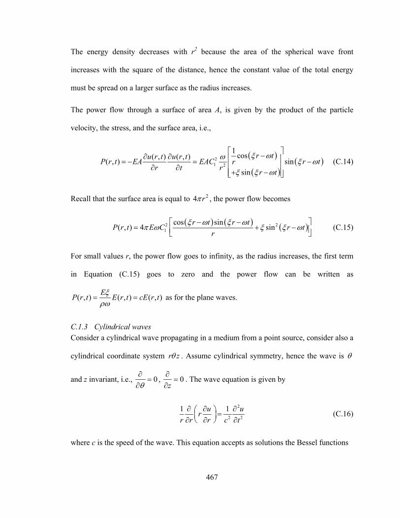
467
The energy density decreases with r2 because the area of the spherical wave front
increases with the square of the distance, hence the constant value of the total energy
must be spread on a larger surface as the radius increases.
The power flow through a surface of area A, is given by the product of the particle
velocity, the stress, and the surface area, i.e.,
( )
( )( )2
1 2
1 cos( , ) ( , )( , ) sinsin
r tu r t u r tP r t EA EAC r trr t r r t
ξ ωω ξ ωξ ξ ω
⎡ ⎤−∂ ∂ ⎢ ⎥= − = −⎢ ⎥∂ ∂ + −⎢ ⎥⎣ ⎦
(C.14)
Recall that the surface area is equal to 24 rπ , the power flow becomes
( ) ( ) ( )2 21
cos sin( , ) 4 sinr t r tP r t E C r tr
ξ ω ξ ωπ ω ξ ξ ω
⎡ ⎤− −= + −⎢ ⎥⎣ ⎦
(C.15)
For small values r, the power flow goes to infinity, as the radius increases, the first term
in Equation (C.15) goes to zero and the power flow can be written as
( , ) ( , ) ( , )EP r t E r t cE r tξρω
= = as for the plane waves.
C.1.3 Cylindrical waves Consider a cylindrical wave propagating in a medium from a point source, consider also a
cylindrical coordinate system r zθ . Assume cylindrical symmetry, hence the wave is θ
and z invariant, i.e., 0θ∂
=∂
, 0z
∂=
∂. The wave equation is given by
2
2 2
1 1u urr r r c t
∂ ∂ ∂⎛ ⎞ =⎜ ⎟∂ ∂ ∂⎝ ⎠
(C.16)
where c is the speed of the wave. This equation accepts as solutions the Bessel functions

468
( ) ( )1 0 2 0( , ) i t i tu r t C J r e C Y r eω ωξ ξ− −= + (C.17)
where C1 and C2 are constant to be determined through the boundary conditions, 0J is the
Bessel function of the first kind and order zero, and 0Y is the Bessel function of the
second kind and order zero. Equation (C.17) can be written in the complex form as
( ) ( ) ( ) ( )1 21 0 2 0( , ) i t i tu r t C H r e C H r eω ωξ ξ− −= + (C.18)
where the Henkel functions are given by
( ) ( ) ( ) ( )( ) ( ) ( ) ( )
10 0 0
20 0 0
H r J r iY r
H r J r iY r
ξ ξ ξ
ξ ξ ξ
= +
= − (C.19)
the first function of Equation (C.19) is for inward propagating modes, while the second is
for outward propagating modes. Consider only an outward propagating mode, Equation
(C.18) can be written as
( ) ( ) ( ) ( )1 0 2 0( , ) cos sinu r t C J r t C Y r tξ ω ξ ω= + (C.20)
For cylindrical coordinates it is not possible to express the wave solution in terms of
D’Alambert solution. The energy density of a cylindrical wave is given by the sum of
kinetic energy and potential energy and being the cylindrical wave only harmonic in time,
potential and kinetic energy are not equal. Potential energy density is given by
( ) ( ) ( ) ( ) ( )
( ) ( ) ( ) ( )
2 22 2 2 22 2 1 1 2 1
1 2 1 1
cos sin1 1( , )2 2 2 sin cos
C J r t C Y r tv r t u
C C J r Y r t t
ξ ω ξ ωρ ξ ρ
ξ ξ ω ω
⎡ ⎤⎡ ⎤ ⎡ ⎤+⎣ ⎦ ⎣ ⎦′ ⎢ ⎥= =⎢ ⎥+⎣ ⎦
(C.21)
Kinetic energy density is given by

469
( ) ( ) ( ) ( )
( ) ( ) ( ) ( )
2 22 2 2 22 2 1 0 2 0
1 2 0 0
sin cos1 12 2 2 sin cos
C J r t C Y r tk u
C C J r Y r t t
ξ ω ξ ωρ ω ρ
ξ ξ ω ω
⎡ ⎤⎡ ⎤ ⎡ ⎤+⎣ ⎦ ⎣ ⎦⎢ ⎥= =⎢ ⎥−⎣ ⎦
& (C.22)
The total energy density is given by the sum of potential end kinetic energy density, i.e.,
( ) ( ) ( )
( ) ( ) ( )
( ) ( ) ( ) ( ) ( ) ( )
2 22 2 2 2 21 1 2 0
2 22 2 2 2 22 1 1 0
2 21 2 1 1 0 0
cos1( , ) sin2
2 sin cos
C J r C Y r t
e r t C Y r C J r t
C C J r Y r J r Y r t t
ξ ξ ω ξ ω
ρ ξ ξ ω ξ ω
ξ ξ ξ ω ξ ξ ω ω
⎡ ⎤⎡ ⎤⎡ ⎤ ⎡ ⎤+⎣ ⎦ ⎣ ⎦⎣ ⎦⎢ ⎥⎢ ⎥⎡ ⎤⎡ ⎤ ⎡ ⎤= + +⎣ ⎦ ⎣ ⎦⎣ ⎦⎢ ⎥⎢ ⎥⎡ ⎤+ −⎣ ⎦⎣ ⎦
(C.23)
The terms in Equation (C.23) that depend on the radial direction varies with r as shown
( )2 rπ , see Figure C.2. The energy density amplitude decreases with the radial distance
from the sources as function proportional to ( )1 rπ .
Figure C.2 Energy density amplitude variation with distance from source. Solid lines: Bessel
functions; Dash line: functions proportional to ( )2 rπ
However, the total energy is constant; this is given by the energy density per area of
the wave front. The wave front area per unit width is equal to the area of the circle of
radius r, i.e., 2 rπ , hence the total energy is given by
0 10 20 30 40 50
0.05
0.1
0 10 20 30 40 50
0.05
0.1
rξ rξ
( ) 20a J rξ⎡ ⎤⎣ ⎦
( ) ( )0 02cJ r Y rξ ξ
( ) 20b Y rξ⎡ ⎤⎣ ⎦
( ) 21a J rξ⎡ ⎤⎣ ⎦
( ) ( )1 12cJ r Y rξ ξ
( ) 21b Y rξ⎡ ⎤⎣ ⎦
2arπ 2a
rπ
2brπ
2brπ
2crπ
2crπ

470
( ) ( ) ( )
( ) ( ) ( )
( ) ( ) ( ) ( ) ( )
2 22 2 2 2 21 1 2 0
2 22 2 2 2 22 1 1 0
2 21 2 1 1 0 0
cos
( , ) 2 sin
sin 2
C J r C Y r t
E r t re r C Y r C J r t
C C J r Y r J r Y r t
ξ ξ ω ξ ω
π π ρ ξ ξ ω ξ ω
ξ ξ ξ ω ξ ξ ω
⎡ ⎤⎡ ⎤⎡ ⎤ ⎡ ⎤+⎣ ⎦ ⎣ ⎦⎣ ⎦⎢ ⎥⎢ ⎥⎡ ⎤⎡ ⎤ ⎡ ⎤= = + +⎣ ⎦ ⎣ ⎦⎣ ⎦⎢ ⎥⎢ ⎥⎡ ⎤+ −⎣ ⎦⎣ ⎦
(C.24)
With the use of consideration in Figure C.2, the total energy can be written as
( ) ( ) ( ) ( )
( ) ( )
2 2 2 2 2 2 2 2 2 21 2 2 1
2 21 2
cos sin( , ) 2
sin 2
C C t C C tE r t
C C t
ξ ω ω ξ ω ωρ
ξ ω ω
⎡ ⎤+ + +≈ ⎢ ⎥
+ −⎢ ⎥⎣ ⎦ (C.25)
The energy density decreases with r because the area of the cylinder wave front increases
linearly with the distance from the source, hence the constant value of the total energy
must be spread on a larger surface as the radius increases.
The power flow through a surface of area A, is given by the product of the particle
velocity, the stress, and the surface area, i.e.,
( ) ( )
( ) ( )( ) ( )
( ) ( )1 1 1 0
2 1 2 0
cos sin( , ) ( , )( , )sin cos
C J r t C J r tu r t u r tP r t EA EAr t C Y r t C Y r t
ξ ω ξ ωξω
ξ ω ξ ω
⎡ ⎤ ⎡ ⎤−∂ ∂= − = ⎢ ⎥ ⎢ ⎥
∂ ∂ + +⎣ ⎦ ⎣ ⎦ (C.26)
or after rearrangement
( ) ( ) ( ) ( ) ( ) ( )
( ) ( ) ( ) ( ) ( ) ( )
2 22 0 1 1 0 1
2 21 2 1 0 0 1
sin cos( , )
cos sin
C Y r Y r C J r J r t tP r t EA
C C J r Y r t J r Y r t
ξ ξ ξ ξ ω ωξω
ξ ξ ω ξ ξ ω
⎡ ⎤⎡ ⎤−⎣ ⎦⎢ ⎥=⎡ ⎤⎢ ⎥+ −⎣ ⎦⎣ ⎦
(C.27)
Note that ( ) ( )0 1Y r Y rξ ξ and ( ) ( )0 1J r J rξ ξ varies as ( )1 rπ , while ( ) ( )1 0J r Y rξ ξ and
( ) ( )0 1J r Y rξ ξ− as ( )2 rπ . Recall that the surface area is equal to 2 rπ , hence the power
flow becomes
( ) ( ) ( )2 22 1 1 2( ) 2 sin cos 2P t E C C t t C Cξω ω ω⎡ ⎤≈ − +⎣ ⎦ (C.28)
471
C.2 AVERAGE POWER FLOW
C.2.1 Basic definitions Let consider two media separated by a surface S. The force exerted by medium 1 on
medium 2 is dS− ⋅T n and the power delivered through dS from medium 1 to medium 2
is dS− ⋅ ⋅v T n where v is the velocity field, T is the stress tensor of 2nd rank, and n is the
normal direction to the surface S (see Figure 4.1). The power flow density in the direction
of n is
⋅ = − ⋅ ⋅P n v T n (C.29)
where the acoustic Poynting vector P is defined as
= − ⋅P v T (C.30)
Let v and T be time harmonic, hence their expression is
( )( )
0
0
( ) cos
( ) cosv
v
t t
t t
ω φ
ω φ
= +
= +
v v
T T (C.31)
where 30 ∈v 3 3
0 ∈ ×T are real amplitudes. Note that ( )tv and ( )tT are not
necessarily in phase, i.e., v Tφ φ≠ . Substitution of Equation (C.31) into Equation (C.30)
yields
( ) ( )0 0( ) ( ) ( ) cos cosv Tt t t t tω φ ω φ− = ⋅ = ⋅ + +P v T v T (C.32)
Recall the trigonometric identities
cos( ) cos cos sin sin2cos cos cos( ) cos( )
a b a b a ba b a b a b± =
= − + +m
(C.33)
In view of Equation (C.33), we can write Equation (C.32) as

472
( ) ( )
( ) ( )
10 02
1 10 0 0 02 2
( ) cos cos 2
cos cos 2v T v T
v T v T
t t
t
φ φ ω φ φ
φ φ ω φ φ
⎡ ⎤− = ⋅ − + + +⎣ ⎦= ⋅ − + ⋅ + +
P v T
v T v T (C.34)
The function ( )tP defined by Equation (C.34) is a harmonic function that contains a
constant part, ( )10 02 cosactive v Tφ φ− = ⋅ −P v T , and a harmonic part
( )10 02 cos 2reactive v Ttω φ φ− = ⋅ + +P v T that oscillates with twice the frequency of the
original variables given by Equation (C.31). To calculate the time-average value of ( )tP ,
we use the formula
( ) ( )1 1 1
0 020( ) cos cos 2
T
av v T v TT Tt dt tφ φ ω φ φ− = − = − + + +∫P P v T
( )0
10 02 cos
T
v T
dt
φ φ
⎡ ⎤⎣ ⎦
= −
∫v T
(C.35)
where T is the period of oscillation, 2 /T π ω= . Note that the time-averaged value equals
the active part, i.e., av active=P P .
C.2.2 Complex notations To take advantage of complex notations, we will utilize the implied convention that only
the real part of the complex exponential function is used, i.e.,
( ) ( )( )( ) ( )( )
0 0
0 0
( ) cos Re
( ) cos Re
v
T
i tv
i tT
t t e
t t e
ω φ
ω φ
ω φ
ω φ
+
+
= + =
= + =
v v v
T T T (C.36)
where we have used the Euler formulae, i.e.,
cos
2
ix ixe ex−+
=,
sin2
ix ixe exi
−−=
(C.37)
Define the complex variables

473
( )
( )0
0
( )
( )
v
T
i t
i t
t e
t e
ω φ
ω φ
+
+
=
=
v v
T T (C.38)
and the complex amplitudes
0 0
0 0
v
T
i
i
e
e
φ
φ
=
=
v v
T T (C.39)
We can rewrite Equation (C.36) with the use of Equations (C.38), (C.39), i.e.,
( )( ) ( ) ( )( )( ) ( ) ( )
0 0 0
0 0 0
( ) Re Re Re
( ) Re Re Re
v v
T T
i t i i t i t
i t i i t i t
t e e e e
t e e e e
ω φ φ ω ω
ω φ φ ω ω
+
+
= = =
= = =
v v v v
T T T T (C.40)
In view of the relation between Equations (C.31) and (C.40), we will use interchangeably
the cosinusoidal formulation of Equation (C.31) and the complex formulation of Equation
(C.40); when referring to the complex formulation of Equation (C.40), the Re sign will be
implied, but not explicitly written.
Equation (C.35) can be written in complex notations as
[ ] ( ) ( )( )
( )( ) ( )1 1
0 0 0 02 2
1 10 0 0 02 2
( ) ( ) cos Re
Re Re
v T
v T
iav v Tav
i i
t t e
e e
φ φ
φ φ
φ φ −
−
− = ⋅ = ⋅ − = ⋅
⎡ ⎤= = ⋅⎣ ⎦
P v T v T v T
v T v T% (C.41)
where T% is the complex conjugate of T . Equation (C.41) can be expressed in terms of
the complex variables of Equation (C.38) using the products ( ) ( )t tv T% and ( ) ( )t tv T%% .
Since the harmonic exponential i te ω is common in both variables, the products ( ) ( )t tv T%
and ( ) ( )t tv T%% do not contain it because i te ω and i te ω− cancel out, e.g.,
0 0 0 0( ) ( ) i t i tt t e eω ω−= ⋅ = ⋅v T v T v T% % % (C.42)

474
Using Equation (C.42), we can write Equation (C.41) as
[ ] ( )1 10 02 2( ) ( ) Re Re ( ) ( )av av
t t t t⎡ ⎤− = ⋅ = ⋅ = ⋅⎣ ⎦P v T v T v T% % (C.43)
Equation (C.43) indicates the general result that the time–averaged product of two
complex harmonic variables is the real part of half the product between one variable and
the conjugate of the other variable, i.e.,
[ ] 1 12 2( ) ( ) Re ( ) ( ) Re ( ) ( )
avt t t t t t⎡ ⎤ ⎡ ⎤⋅ = ⋅ = ⋅⎣ ⎦⎣ ⎦v T v T v T% % (C.44)
In view of the above, we define the complex Poynting vector, i.e.,
( )1 1 1
0 0 0 0 0 02 2 21 1
0 0 0 02 2cos( ) sin( )
v v TTi ii
v T v T
e e ei
φ φ φφ
φ φ φ φ
−−− = ⋅ = = ⋅
= ⋅ − + ⋅ −
P v T v T v Tv T v T
% % (C.45)
The real part of the complex Poynting vector equals the time-averaged Poynting vector,
Reav =P P (active Poynting factor). The magnitude of the complex Poynting vector
equals the peak value of the oscillating part of the reactive Poynting vector,
Impeakreactive =P P .

475
D ORTHOGONALITY FOR VIBRATION AND WAVE PROBLEMS
D.1 ORTHOGONALITY PROOF FOR SOME VIBRATION PROBLEMS
D.1.1 Straight-crested axial vibration of rectangular plates
The problem is y-invariant and depends only on x, i.e.,
( , , ) ( , )( , , ) 0
u x y t u x tv x y t
→≡
(D.1)
The wave equation for this particular problem is
2Lc u u′′ = && (D.2)
where ( )2
21LEc
ρ ν=
−. Assume that the solution is time harmonic, such as,
ˆ( , ) ( ) i tu x t u x e ω= (D.3)
Equation (D.2) becomes
2ˆ ˆ 0Lu uγ′′ + = (D.4)
where the wavenumber is defined as 2
22LLc
ωγ = . Solution to Equation (D.4) is given by
ˆ( ) sin cosL Lu x A x B xγ γ= + (D.5)

476
where A and B are constant to be determined through the boundary conditions. Assume
that the boundary conditions for the rectangular plate are stress free conditions at the
edges. Recall that
2 ( , )1
d
x xxd
EhN dy u x tσν−
′= =−∫ (D.6)
Hence the boundary conditions are
(0, ) 0( , ) 0
u tu l t
′ =⎧⎨ ′ =⎩
(D.7)
Substitute Equation (D.5) into the boundary conditions and solve to get
0sin 0L L
AB lγ γ
=⎧⎨ =⎩
(D.8)
System (D.8) is verified for
nLnlπγ = (D.9)
With the use of (D.8) and (D.9), Equation (D.5) can be written as
( )( , ) cos i tn nL
nu x t B x e ωγ= ∑ (D.10)
Consider two separate mode shapes, ( )pU x and ( )qU x , such as they satisfy Equation
(D.2) and (D.8) i.e.,
2 2
2 2
L p p p
L q q q
c U U
c U U
ω
ω
′′ = −
′′ = − (D.11)
Multiply the fist of Equation (D.11) by ( )qU x and the second by ( )pU x , hence

477
2 2
2 2
L p q p p q
L q p q q p
c U U U U
c U U U U
ω
ω
′′ = −
′′ = − (D.12)
Integrate both equations over the area. Since the problem is y-invariant, we only need to
integrate over x, i.e.
2 2
0 0
2 2
0 0
l l
L p q p p q
l l
L q p q q p
c U U dx U U dx
c U U dx U U dx
ω
ω
′′ = −
′′ = −
∫ ∫
∫ ∫ (D.13)
Integrate by part
2 2 20
0 0
2 2 20
0 0
l llL p q L p q p p q
l llL q p L q p q q p
c U U c U U dx U U dx
c U U c U U dx U U dx
ω
ω
′ ′ ′− = −
′ ′ ′− = −
∫ ∫
∫ ∫ (D.14)
Subtract the first line from the second
( ) ( )2 2 2
00
llL p q q p p q p qc U U U U U U dxω ω′ ′− = − − ∫ (D.15)
From the boundary conditions (D.8) we obtain
( )2 2
0
0l
p q p qU U dxω ω− =∫ (D.16)
For distinct mode numbers, p q≠ , the frequencies are also distinct, 2 2p qω ω≠ , and hence
Equation (D.16) implies
0
0l
p qU U dx =∫ , p q≠ (D.17)

478
this is the orthogonality condition. To derive the normalization factor, consider two
distinct solutions given by Equation (D.10), i.e.,
( ) cos
( ) cosp p pL
p q qL
U x B x
U x B x
γ
γ
=
= (D.18)
Substitute Equation (D.18) into the orthogonality relation (D.17) and solve the integral to
get
( ) ( )0
sin sincos cos
2
lmL nL mL nLm n
m n mL nLmL nL mL nL
l lB BB B x xdxγ γ γ γ
γ γγ γ γ γ
⎡ ⎤+ −= +⎢ ⎥+ −⎣ ⎦
∫ (D.19)
Note that
( )
( )
mL nL
mL nL
m nl
m nl
πγ γ
πγ γ
⎧ + = +⎪⎪⎨⎪ − = −⎪⎩
(D.20)
Substitution of Equation (D.20) into Equation (D.19) yields
( ) ( )
0
sin sincos cos2
lm n
m n mL nLB B l m n m nB B x xdx
m n m nπ πγ γ
π⎡ ⎤+ −
= +⎢ ⎥+ −⎣ ⎦∫ (D.21)
i. For m n≠ 0
cos cos 0l
m n mL nLB B x xdxγ γ =∫
i. For m n= 0
sin 2cos cos2 2
lm n
m n mL nLB B l nB B x xdx
nπγ γ
π=∫
( )sin m nm n
π−+
−
2
2nB l
π⎡ ⎤⎢ ⎥ =⎢ ⎥⎣ ⎦
.
The normalization factor is 2nB l= .

479
D.1.2 Axial vibration of circular plates
Assume that the problem is axial symmetric, hence θ -invariant and it depends only on r,
i.e., ( , , ) ( , )u r t u r tθ → and ( , , ) 0v r tθ ≡ . The wave equation for this particular problem is
22
1L
uc u u ur r
⎛ ⎞′′ ′+ − =⎜ ⎟⎝ ⎠
&& (D.22)
where ( )2
21LEc
ρ ν=
−. Assume that the solution is time-harmonic, such as,
ˆ( , ) ( ) i tu r t u r e ω= . Equation (D.22) becomes
( )2 2 2ˆ ˆ ˆ1 0r u ru r uγ′′ ′+ + − = (D.23)
where the wavenumber is defined as 2
22Lc
ωγ = . Perform the following change of variable
x rγ= (D.24)
and recall that
2 2 2
dx dr
dx dr
γ
γ
=
= (D.25)
Equation (D.23) becomes
( )2 2ˆ ˆ ˆ1 0x u xu x u′′ ′+ + − = (D.26)
Solution to Equation (D.26) is given by
( ) ( )1 1ˆ( )u x AJ x BY x= + (D.27)
However the Bessel function of the second kind has infinite value at 0x rγ= = and has
to be discarded. Equation (D.27) becomes

480
( )1ˆ( )u r AJ rγ= (D.28)
where A is a constant to be determined from the boundary conditions. We assume that the
boundary conditions are
2( , )( ) ( , ) 0
1
d
r rrd
Eh u a tN a dy u a ta
σ νν−
⎛ ⎞′= = + =⎜ ⎟⎝ ⎠−∫ (D.29)
Substitute Equation (D.28) into (D.29) and obtain
( )( )
( )2 11 0A J a J a
aνγ γ γ⎛ ⎞+
− + =⎜ ⎟⎝ ⎠
(D.30)
Equation (D.30) is verified for
( ) ( ) ( )2 11 0aJ a J aγ γ ν γ− + = (D.31)
Considering the boundary conditions (D.31), solution (D.28) can be written as
( )1ˆ( ) n nn
u r A J rγ= ∑ (D.32)
where nγ satisfies Equation (D.31).
Consider two separate mode shapes, ( )pU r and ( )qU r , such as they satisfy Equation
(D.22) and (D.29) i.e.,
2 2
2 2
pL p p p p
qL q q q q
Uc rU U rU
rU
c rU U rUr
ω
ω
⎛ ⎞′′ ′+ − = −⎜ ⎟
⎝ ⎠⎛ ⎞
′′ ′+ − = −⎜ ⎟⎝ ⎠
(D.33)
Multiply the fist of Equation (D.33) by ( )qU r and the second by ( )pU r , hence

481
2 2
2 2
p qL p q p q p p q
q pL q p q p q q p
U Uc rU U U U rU U
rU U
c rU U U U rU Ur
ω
ω
⎛ ⎞′′ ′+ − = −⎜ ⎟
⎝ ⎠⎛ ⎞
′′ ′+ − = −⎜ ⎟⎝ ⎠
(D.34)
Integrate over the area. Since the problem is axisymmetric, we only need to integrate
radially, i.e.
2 2
0 0
2 2
0 0
a ap q
L p q p q p p q
a aq p
L q p q p q q p
U Uc rU U U U dr rU U dr
r
U Uc rU U U U dr rU U dr
r
ω
ω
⎛ ⎞′′ ′+ − = −⎜ ⎟
⎝ ⎠
⎛ ⎞′′ ′+ − = −⎜ ⎟
⎝ ⎠
∫ ∫
∫ ∫ (D.35)
Integrate by part and rearrange the terms to get
2 2 20
0 0
2 2 20
0 0
a aa p qL p q L p q p p q
a aa q pL q p L q p q q p
U Uc rU U c rU U dr rU U dr
r
U Uc rU U c rU U dr rU U dr
r
ω
ω
⎛ ⎞′ ′ ′+ − − = −⎜ ⎟
⎝ ⎠
⎛ ⎞′ ′ ′+ − − = −⎜ ⎟
⎝ ⎠
∫ ∫
∫ ∫ (D.36)
Subtract the first line from the second, i.e.,
( ) ( )2 2 2
00
aaL p q q p p q p qc a U U U U rU U drω ω′ ′− = − − ∫ (D.37)
Note that from (D.29)
( , )( , ) 0
( , )( , ) 0
pp q
qq p
u a tu a t u
au a t
u a t ua
ν
ν
′ + = ×
′ + = × −
(D.38)
Sum the equations in (D.38) to obtain

482
( )p q q p p q q pau u u u u u u u
aν′ ′− + −( ) 0
a= (D.39)
hence
( ) 0p q q p au u u u′ ′− = (D.40)
With the use of Equation (D.40), Equation (D.37) becomes
( )2 2
0
0a
p q p qrU U drω ω− =∫ (D.41)
For same mode shapes (p=q) the equation is verified, for different mode shapes ( p q≠ )
we should have
0
0a
q prU U dr =∫ (D.42)
Note that for the specific solution (D.32) Equation (D.41) becomes
( ) ( ) ( )2 21 1
0
0a
q p p q p qA A rJ r J r drω ω γ γ− =∫ (D.43)
For p q≠ the integral is equal to 0, for p q=
( ) ( ) ( )
( ) ( ) ( )
222 2 2 2 21 1 12 2
0 02
2 2 2 2 2 2 21 12
1 12
2
aa
q q q q qq
qq q q q
q
A r J r dr A r J r J rr
Aa J a a J a
νγ γ γγ
γ ν γ γ γγ
⎡ ⎤⎧ ⎫⎛ ⎞⎪ ⎪′⎡ ⎤ = − + =⎢ ⎥⎜ ⎟⎨ ⎬⎣ ⎦ ⎜ ⎟⎢ ⎥⎪ ⎪⎝ ⎠⎩ ⎭⎣ ⎦
⎡ ⎤′− +⎣ ⎦
∫ (D.44)
with nγ is a real zero of Equation (D.31).

483
D.1.3 Flexural vibration of rectangular plates
D.1.3.1 Infinite aspect ratio (straight-crested flexural vibration)
Consider a plate with infinite aspect ratio. The problem is assumed to be y-invariant and
the wave equation is
4Fc w w′′′′ = − && (D.45)
where 4F
Dchρ
= . Solution to Equation (D.45) is
( )1 2 3 4( , ) F F F Fi x i x x x i tw x t A e A e A e A e eγ γ γ γ ω− −= + + + (D.46)
where FFc
ωγ = . Assume the following boundary conditions for a supported plate, i.e.,
(0, ) 0( , ) 0
(0, ) (0, ) 0( , ) ( , ) 0
x
x
w tw a tM t Dw tM a t Dw a t
=⎧⎪ =⎪⎨ ′′= − =⎪⎪ ′′= − =⎩
(D.47)
Substitute Equation (D.46) into (D.47) and rearrange the terms.
1 2 3 4
1 2 3 42 2 2 2
1 2 3 42 2 2 2
1 2 3 4
0
0
0
0
F F F F
F F F F
i a i a a a
F F F Fi a i a a a
F F F F
A A A A
A e A e A e A e
A A A A
A e A e A e A e
γ γ γ γ
γ γ γ γ
γ γ γ γ
γ γ γ γ
− −
− −
+ + + =⎧⎪
+ + + =⎪⎨
− − + + =⎪⎪− − + + =⎩
(D.48)
A non trivial solution to system (D.48) is found if the determinant of the characteristic
equation is equal to zero, i.e.,

484
2 2 2 2
2 2 2 2
1 1 1 1
0F F F F
F F F F
i a i a a a
F F F Fi a i a a a
F F F F
e e e e
e e e e
γ γ γ γ
γ γ γ γ
γ γ γ γ
γ γ γ γ
− −
− −
=− −
− −
(D.49)
Solution of the determinant yields ( )( )44 0F F F Fa a i a i aF e e e eγ γ γ γγ − −− − = , hence
sinh sin 0F Fa aγ γ = or
Fnnaπγ = (D.50)
Consider two separate mode shapes, ( )pW x and ( )qW x , such as they satisfy Equation
(D.45) and boundary conditions (D.47). Multiply the fist of equation by ( )qW x and the
second by ( )pW x , i.e.,
4 2
4 2
ivF p q p p q
ivF q p q q p
c W W W W
c W W W W
ω
ω
⎧ =⎪⎨
=⎪⎩ (D.51)
Integrate through the length of the plate to get
4 2
0 0
4 2
0 0
a aiv
F p q p p q
a aiv
F q p q q p
c W W dx W W dx
c W W dx W W dx
ω
ω
⎧=⎪
⎪⎨⎪ =⎪⎩
∫ ∫
∫ ∫ (D.52)
Perform integration by parts and obtain
4 2
0 0
4 2
0 0
a a
F p q p p q
a a
F q p q q p
c W W dx W W dx
c W W dx W W dx
ω
ω
⎧′′ ′′ =⎪
⎪⎨⎪ ′′ ′′ =⎪⎩
∫ ∫
∫ ∫ (D.53)

485
Subtract the two equations to get
( )2 2
0
0a
p q p qW W dxω ω− =∫ (D.54)
This is the orthogonality relation for a simply supported plate with infinite aspect ratio.
D.1.3.2 General flexural vibration of simply supported plate
Consider a rectangular plate with infinite aspect ratio, the wave equation is
( )4 4 0wγ∇ − = (D.55)
Boundary conditions for a free plate are given by
(0, ) 0( , ) 0( ,0) 0( , ) 0
w yw a yw xw x b
=⎧⎪ =⎪⎨ =⎪⎪ =⎩
( )( )( )( )
0, 0
, 0
,0 0
, 0
x
x
y
y
M y
M a y
M x
M x b
⎧ =⎪
=⎪⎨ =⎪⎪ =⎩
(D.56)
Solution to Equation (D.55) is written as
( , , ) sin sini tmn
m x n yw x y t A ea b
ω π π= (D.57)
Rewrite Equation (D.55) in a more extended form, i.e.,
4 4 4
4 24 2 2 42Fw w wc w
x x y yω
⎛ ⎞∂ ∂ ∂+ + =⎜ ⎟
∂ ∂ ∂ ∂⎝ ⎠ (D.58)
Consider two separate mode shapes, ( )pW x and ( )qW x , such as they satisfy Equation
(D.58) and boundary conditions (D.56). Multiply the fist of equation (D.58) by ( )qW x
and the second by ( )pW x , i.e.,

486
4 4 44 2
4 2 2 4
4 4 44 2
4 2 2 4
2
2
p p pF q q q p p q
q q qF p p p q q p
W W Wc W W W W W
x x y y
W W Wc W W W W W
x x y y
ω
ω
⎧ ⎛ ⎞∂ ∂ ∂⎪ + + =⎜ ⎟⎜ ⎟∂ ∂ ∂ ∂⎪ ⎝ ⎠⎨
⎛ ⎞∂ ∂ ∂⎪+ + =⎜ ⎟⎪ ⎜ ⎟∂ ∂ ∂ ∂⎝ ⎠⎩
(D.59)
Integrate through the length of the plate to get
4 4 44 2
4 2 2 40 0 0 0
4 4 44 2
4 2 2 40 0 0 0
2
2
a b a bp p p
F q q q p p q
a b a bq q q
F p p p q q p
W W Wc W W W dydx W W dydx
x x y y
W W Wc W W W dydx W W dydx
x x y y
ω
ω
⎧ ⎛ ⎞∂ ∂ ∂⎪ + + =⎜ ⎟⎜ ⎟∂ ∂ ∂ ∂⎪ ⎝ ⎠⎨
⎛ ⎞∂ ∂ ∂⎪+ + =⎜ ⎟⎪ ⎜ ⎟∂ ∂ ∂ ∂⎝ ⎠⎩
∫ ∫ ∫ ∫
∫ ∫ ∫ ∫ (D.60)
Perform integration by parts and obtain
2 2 2 2 2 24 2
2 2 2 20 0 0 0
2 2 2 2 2 24 2
2 2 2 20 0 0 0
2
2
a b a bp q p q p q
F p p q
a b a bq p q p q p
F q q p
W W W W W Wc dydx W W dydx
x y x yx x y y
W W W W W Wc dydx W W dydx
x y x yx x y y
ω
ω
⎧ ⎛ ⎞∂ ∂ ∂ ∂ ∂ ∂⎪ + + =⎜ ⎟⎜ ⎟∂ ∂ ∂ ∂∂ ∂ ∂ ∂⎪ ⎝ ⎠⎨
⎛ ⎞∂ ∂ ∂ ∂ ∂ ∂⎪− + =⎜ ⎟⎪ ⎜ ⎟∂ ∂ ∂ ∂∂ ∂ ∂ ∂⎝ ⎠⎩
∫ ∫ ∫ ∫
∫ ∫ ∫ ∫ (D.61)
Subtract the two equations to obtain the orthogonality relation for a rectangular plate, i.e.,
( )2 2
0 0
0a b
p q p qW W dydxω ω− =∫ ∫ (D.62)
D.1.4 Flexural vibration of circular plates
Consider a circular plate in a cylindrical coordinate system. The equation of motion for a
circular plate is given by
4 0D w hwρ∇ + =&& (D.63)
Assume time-harmonic vibrations and expand the bi-harmonic operator assuming θ -
invariance

487
4 3 2
4 24 3 2 2 3
2 1 1Fc w w
r rr r r r rω
⎛ ⎞∂ ∂ ∂ ∂+ − + =⎜ ⎟∂∂ ∂ ∂⎝ ⎠
(D.64)
Assume that the circular plate is a free plate such as the boundary conditions are
( )3 2
23 2 2
1 1( ) 0ra a
w w wV a wr r rr r r
⎛ ⎞∂ ∂ ∂ ∂= ∇ = + − =⎜ ⎟∂ ∂∂ ∂⎝ ⎠
(D.65)
and
2
21( ) 0r
a
w wM a Dr rr
ν⎡ ⎤∂ ∂
= − + =⎢ ⎥∂∂⎣ ⎦ (D.66)
Consider two separate mode shapes, ( , )pW r θ and ( , )qW r θ , such as they satisfy Equation
(D.64) and boundary conditions (D.65) (D.66) and substitute them into Equation (D.64),
i.e.,
4 3 24 2
4 3 2 2 3
4 3 24 2
4 3 2 2 3
2 1 1
2 1 1
F p p p
F q q q
c W Wr rr r r r r
c W Wr rr r r r r
ω
ω
⎛ ⎞∂ ∂ ∂ ∂+ − + =⎜ ⎟∂∂ ∂ ∂⎝ ⎠
⎛ ⎞∂ ∂ ∂ ∂+ − + =⎜ ⎟∂∂ ∂ ∂⎝ ⎠
(D.67)
Multiply the fist of equation (D.67) by ( , )qW r θ and the second by ( , )pW r θ , i.e.,
4 3 24 2
4 3 2 2
4 3 24 2
4 3 2 2
1 12
1 12
p p p pF q p p q
q q q qF p q q p
W W W Wc r W rW W
r rr r r rW W W W
c r W rW Wr rr r r r
ω
ω
⎧ ⎛ ⎞∂ ∂ ∂ ∂⎪ + − + =⎜ ⎟
∂∂ ∂ ∂⎪ ⎝ ⎠⎨
⎛ ⎞∂ ∂ ∂ ∂⎪+ − + =⎜ ⎟⎪ ∂∂ ∂ ∂⎝ ⎠⎩
(D.68)
Integrate through the length of the plate to get

488
4 3 2 2
4 3 2 2 40 0
4 3 2 2
4 3 2 2 40 0
1 12
1 12
a ap p p p p
q p qF
a aq q q q p
p q pF
W W W Wr W dr rW W dr
r rr r r r c
W W W Wr W dr rW W dr
r rr r r r c
ω
ω
⎧ ⎛ ⎞∂ ∂ ∂ ∂⎪ + − + =⎜ ⎟
∂∂ ∂ ∂⎝ ⎠⎪⎨
⎛ ⎞∂ ∂ ∂ ∂⎪+ − + =⎜ ⎟⎪ ∂∂ ∂ ∂⎝ ⎠⎩
∫ ∫
∫ ∫ (D.69)
Perform integration by parts and obtain after rearrangement
3 2 2 2
3 2 2 2 20
2 2 2
2 2 40 0
3 2 2 2
3 2 2 2 2
1 1 1
1
1 1
p p p p q p pq q q q q
a
a ap q p q p
p qF
q q q q p qp p p p
a
W W W W W W Wa W W W W W
a r r r rr r a r r
W W W Wr dr rW W dr
r r rr r c
W W W W W Wa W W W W
a r rr r a r r
ω
⎛ ⎞ ⎛ ⎞∂ ∂ ∂ ∂ ∂ ∂ ∂+ − − + +⎜ ⎟ ⎜ ⎟
∂ ∂ ∂∂ ∂ ∂ ∂⎝ ⎠ ⎝ ⎠
⎛ ⎞∂ ∂ ∂ ∂+ − =⎜ ⎟
∂ ∂∂ ∂⎝ ⎠
⎛ ⎞∂ ∂ ∂ ∂ ∂ ∂+ − − +⎜ ⎟
∂ ∂∂ ∂ ∂ ∂⎝ ⎠
∫ ∫
0
2 2 2
2 2 40 0
1
1
qp
a aq p q p q
q pF
WW
r r
W W W Wr dr rW W dr
r r rr r cω
⎧⎪⎪⎪⎪⎪⎪⎨
⎛ ⎞∂⎪+⎜ ⎟⎪ ∂⎝ ⎠⎪
⎪ ⎛ ⎞∂ ∂ ∂ ∂⎪+ − =⎜ ⎟⎪ ∂ ∂∂ ∂⎝ ⎠⎩
∫ ∫
(D.70)
From the boundary conditions (D.65) and the relation (0) (0) 0W AJ= = , Equation
(D.70) becomes
2 2 2 2
2 2 2 40 0
2 2 2 2
2 2 2 40 0
1
1
a ap q p q p q p
p qa F
a aq p q p q p q
q pa F
W W W W W Wa r dr rW W dr
r r r rr r r c
W W W W W Wa r dr rW W dr
r r r rr r r c
ω
ω
⎧ ⎛ ⎞∂ ∂ ∂ ∂ ∂ ∂⎪− + − =⎜ ⎟
∂ ∂ ∂∂ ∂ ∂⎝ ⎠⎪⎨
⎛ ⎞∂ ∂ ∂ ∂ ∂ ∂⎪− + − =⎜ ⎟⎪ ∂ ∂ ∂∂ ∂ ∂⎝ ⎠⎩
∫ ∫
∫ ∫ (D.71)
Subtract the second of (D.71) from the first to get
( )2 22 2
2 2 40
ap qp q q p
p qa F
W W W Wa rW W dr
r rr r c
ω ω⎛ ⎞ −∂ ∂ ∂ ∂− − =⎜ ⎟
∂ ∂∂ ∂⎝ ⎠ ∫ (D.72)

489
Recall the boundary condition (D.66), substitute the two wave modes ( , )pW r θ and
( , )qW r θ into it and multiply the first by the radial derivative of ( , )pW r θ and the second
by the radial derivative of ( , )qW r θ , i.e.,
2
2
2
2
1 0
1 0
p p q
q q p
W W Wr r rr
W W Wr r rr
ν
ν
∂ ∂ ∂+ = ×
∂ ∂∂∂ ∂ ∂
+ = ×∂ ∂∂
(D.73)
Sum up the equations to obtain
2 2
2 2 0p q q pW W W Wr rr r
∂ ∂ ∂ ∂− =
∂ ∂∂ ∂ (D.74)
Hence Equation (D.72) becomes
( )2 2
0
0a
p q p qrW W drω ω− =∫ (D.75)
D.2 STURM-LIOUVILLE PROBLEM
Consider the homogeneous, second-order, linear equation for the scalar field ψ of the
form
2 2 0kψ ψ∇ + = (D.76)
where k can be either 0, a real constant, or a function of coordinates.
Through separation of variables, Equation (D.76) can be written in the form
[ ]( ) ( ) ( ) 0d dp z q z r zdz dz
ψ λ ψ⎡ ⎤ + + =⎢ ⎥⎣ ⎦ (D.77)
490
This equation is the Liouville equation. Functions p, q, and r are characteristic of the
coordinate used in the separation; p and r are always defined positive. The parameter λ
depends on the boundary conditions. With the use of Equation (D.77) and the procedure
described in Morse et al (1953), we find the orthogonality relation
0b
n ma
rdzψ ψ =∫ (D.78)
If nψ and mψ belong to different eigenvalues ( n mλ λ≠ ) they are orthogonal.
In general, if a problem can be written as in Equation (D.77), the mode solutions form a
set of mutually orthogonal functions.
D.3 ORTHOGONALITY RELATION FROM THE REAL RECIPROCITY RELATION
D.3.1 Orthogonality relation in rectangular coordinates
Assume that solutions 1 and 2 are generic time-harmonic guided-wave modes (e.g., plate
guided waves), i.e.,
1
2
( , , , ) ( )
( , , , ) ( )
n
m
i x i tn
i x i tm
x y z t y e e
x y z t y e e
ξ ω
ξ ω
−
−
=
=
v v
v v (D.79)
In the generic case, the wavenumbers and the amplitudes are assumed to be complex
( ,m nξ ξ ∈ , ,n m ∈v v ). The strains and stress will also be harmonic, i.e.,
1
2
( , , , ) ( )
( , , , ) ( )
n
m
i x i tn
i x i tm
x y z t y e e
x y z t y e e
ξ ω
ξ ω
−
−
=
=
T T
T T (D.80)
Recall the real reciprocity relation for time-harmonic functions as given by Equation
(5.17) and set the source terms equal to zero ( 1 2= =F F 0 ), i.e.,

491
( )2 1 1 2 0∇ ⋅ − ⋅ =v T v T (D.81)
Substitution of Equations (D.79) and (D.80) into Equation (6.104) yields
( ) ( ) ( )
( ) ( )
2 1 1 2 2 1 1 2 2 1 1 2
2 1 2 1 1 2 1 2 2 1 1 2
ˆ ˆ
ˆ ˆ 0n m n m
x y
i i i iy
ξ ξ ξ ξ
∂ ∂∇ ⋅ − ⋅ = ⋅ − ⋅ ⋅ + ⋅ − ⋅ ⋅
∂ ∂∂
= − ⋅ − ⋅ + ⋅ + ⋅ ⋅ + ⋅ − ⋅ ⋅ =∂
v T v T v T v T x v T v T y
v T v T v T v T x v T v T y(D.82)
where x and y are the unit vectors in the x and y directions. Simplification of Equation
(D.82) yields
( )( ) ( )2 1 1 2 2 1 1 2ˆ ˆ 0n miy
ξ ξ ∂− + ⋅ − ⋅ ⋅ + ⋅ − ⋅ ⋅ =
∂v T v T x v T v T y (D.83)
Substitution of Equations (D.79) and (D.80) into Equation (D.83) yields
( ) ( ) ( )
( ) ( )
ˆ( ) ( ) ( ) ( )
ˆ( ) ( ) ( ) ( ) 0
n m
n m
i x i tn m m n n m
i x i tm n n m
i e e v y y y y
e e v y y y yy
ξ ξ ω
ξ ξ ω
ξ ξ − +
− +
− + − ⋅
∂+ − ⋅ =
∂
T v T x
T v T y (D.84)
Since the exponential function ( )n mi x i te eξ ξ ω− + is non zero, we can divide Equation (D.84)
by ( )n mi x i te eξ ξ ω− + and get
( )( )
( )
ˆ( ) ( ) ( ) ( )
ˆ( ) ( ) ( ) ( ) 0
n m m n n m
m n n m
i y y y y
y y y yy
ξ ξ− + − ⋅
∂+ − ⋅ =
∂
v T v T x
v T v T y (D.85)
Integrate Equation (D.85) with respect to y to get
( ) ( ) ( )ˆ ˆ( ) ( ) ( ) ( ) ( ) ( ) ( ) ( )d
d
n m m n n m m n n m dd
i y y y y dy y y y yξ ξ−
−
− + − ⋅ = − − ⋅∫ v T v T x v T v T y (D.86)

492
If boundary conditions in Equation (D.86) at y d= ± are either traction free ( ˆ⋅ =T y 0 ) or
rigid ( =v 0 ), then the right-hand side of Equation (D.86) vanishes and we get
( ) ( ) ˆ( ) ( ) ( ) ( ) 0d
n m m n n md
i y y y y dyξ ξ−
− + − ⋅ =∫ v T v T x (D.87)
If m n nξ ξ ξ−≠ − = , then one can divide by ( )n mξ ξ+ and Equation (D.87) becomes the
orthogonality relation, i.e.,
( ) ˆ( ) ( ) ( ) ( ) 0d
m n n md
y y y y dy−
− ⋅ =∫ v T v T x for m nξ ξ≠ − (D.88)
The wavenumbers of guided waves always occur in pairs having equal value and
opposite signs. By convention, the modes that propagate or decay in the x+ direction are
numbered with positive integers (and negative integers for those in x− direction).
If the m n≠ − , then 0n mξ ξ+ ≠ ; one may divide Equation (D.87) by ( )n mξ ξ− and get
( ) ˆ( ) ( ) ( ) ( ) 0d
m n n md
y y y y dy−
− ⋅ =∫ v T v T x for m n≠ − (D.89)
This is the orthogonality relation for undamped propagating modes.
If m n= − , then 0n m n n n nξ ξ ξ ξ ξ ξ−+ = + = − = and relation (D.88) no longer applies. In
this case ( ) ˆ( ) ( ) ( ) ( )d
m n n md
y y y y dy−
− ⋅∫ v T v T x is nonzero. The orthogonality relation from
the real reciprocity relation relates the wave propagating in the forward direction with
that propagating in the backward direction.

493
Note that the derivation of the orthogonality relation is valid for Lamb wave propagating
in layered waveguide structures, where the material has arbitrary anisotropy, but the
properties of the media are z-invariant.
D.3.2 Orthogonality relation in cylindrical coordinates
For circular crested wave it is not possible to derive a generic formulation of the
orthogonality relation. We directly derive the relation for the case of SH waves and Lamb
waves.
D.3.2.1 Shear horizontal waves
Recall the real reciprocity relation of Equation (5.74) and set the source terms equal to
zero ( 1 2= =F F 0 ), hence
( ) ( )1 2 2 1 1 2 2 1 0r r z zr v T v T r v T v Tr zθ θ θ θ θ θ θ θ
∂ ∂⎡ ⎤− + − =⎣ ⎦∂ ∂ (D.90)
Integrate Equation (D.90) with respect to z to get
( ) ( )1 2 2 1 1 2 2 1 0d
d
r r z z dd
r v T v T dz r v T v Tr θ θ θ θ θ θ θ θ −
−
∂ ⎡ ⎤− + − =⎣ ⎦∂ ∫ (D.91)
Since the shear wave modes satisfy the stress free boundary conditions ( 0zTθ = ), the
right-hand side of Equation (D.91) vanishes and we get
( )1 2 2 1 0d
r rd
r v T v T dzr θ θ θ θ
−
∂ ⎡ ⎤− =⎣ ⎦∂ ∫ (D.92)
Let assume that solutions 1 and 2 are free modes such that (from Equation (3.67)):
1
1 12
2 1
( , ) ( , ) ( ) ( )
( , ) ( , ) ( ) ( )n n
m m
r z v r z i Z z J r
r z v r z i Z z J rθ
θ
ω ξ
ω ξ
= =
= =
v
v (D.93)

494
where ( ) sin cosrZ z v T A z B zθ θ η η= = = + and, from Equation (3.75),
1 11 0
2 12 0
( )( , ) ( ) ( ) 2
( )( , ) ( ) ( ) 2
nr n n n
mr m m m
J rr z T Z z J rr
J rr z T Z z J rr
θ
θ
ξμ ξ ξ
ξμ ξ ξ
⎛ ⎞= = −⎜ ⎟⎝ ⎠⎛ ⎞= = −⎜ ⎟⎝ ⎠
T
T (D.94)
Substitute Equations (D.93) and (D.94) into (D.92) to get
11 0
11 0
( )( ) ( ) 20
( )( ) ( ) 2
md n n m m m
d nm m n n n
J ri Z J r Z J rrr dz
r J ri Z J r Z J rr
ξωμ ξ ξ ξ
ξωμ ξ ξ ξ−
⎡ ⎤⎛ ⎞⎛ ⎞−⎜ ⎟⎢ ⎥⎜ ⎟∂ ⎝ ⎠⎢ ⎥⎜ ⎟ =⎢ ⎥∂ ⎜ ⎟⎛ ⎞− −⎜ ⎟⎜ ⎟⎢ ⎥⎝ ⎠⎝ ⎠⎣ ⎦
∫ (D.95)
Rearrange the terms and factor out the product m nZ Z , i.e.,
( )0 1 1 0( ) ( ) ( ) ( ) 0d
m m n n m n m nd
i r J r J r J r J r Z Z dzr
ωμ ξ ξ ξ ξ ξ ξ−
∂⎡ ⎤− =⎣ ⎦∂ ∫ (D.96)
Bring out of the z integral the terms dependent on r, divide by the term iωμ , and perform
the derivative with respect to r, to get
( )2 21 1( ) ( ) 0
d
n m m n m nd
r J r J r Z Z dzξ ξ ξ ξ−
− =∫ (D.97)
iii. If n m≠ , then ( )2 2 0n mξ ξ− ≠ ; hence 0d
m nd
Z Z dz−
=∫ .
iv. If n m= , then ( )2 2 0n mξ ξ− ≠ and ( )2 0d
md
Z dz−
≠∫ . This is the normalization factor.

495
D.3.2.2 Lamb waves
Recall the real reciprocity relation of Equation (5.81) and set the source terms equal to
zero ( 1 2= =F F 0 ), hence
( ) ( ) ( )2 1 2 1 1 2 1 2 2 1 2 1 1 2 1 2 0r rr z rz r rr z rz r rz z zz r rz z zzr v T v T v T v T r v T v T v T v Tr z
∂ ∂⎡ ⎤ ⎡ ⎤+ − − + + − + =⎣ ⎦ ⎣ ⎦∂ ∂ (D.98)
Integrate Equation (6.133) with respect to z to get
( ) ( ) ( )2 1 2 1 1 2 1 2 2 1 2 1 1 2 1 2 0d d
r rr z rz r rr z rz r rz z zz r rz z zz dd
r v T v T v T v T dz r v T v T v T v Tr −
−
∂ ⎡ ⎤ ⎡ ⎤+ − − + + − + =⎣ ⎦ ⎣ ⎦∂ ∫ (D.99)
Since the Lamb wave modes satisfy the stress free boundary conditions ( 0rz zzT T= = ),
the right-hand side of Equation (D.99) vanishes and we get
( )2 1 2 1 1 2 1 2 0d
r rr z rz r rr z rzd
r v T v T v T v T dzr −
∂ ⎡ ⎤+ − − =⎣ ⎦∂ ∫ (D.100)
Let assume that solutions 1 and 2 are free modes of non-dissipative Lamb waves such
that
( ) ( )( ) ( )
1 11 1 0
2 22 1 0
ˆ ˆˆ ˆ( , ) ( ) ( ) ( ) ( )
ˆ ˆˆ ˆ( , ) ( ) ( ) ( ) ( )
r zr z n n n n
r zr z m m m m
r z v v v z J r v z J r
r z v v v z J r v z J r
ξ ξ
ξ ξ
= + = +
= + = +
v r z r z
v r z r z (D.101)
where from Equations (3.122) and (3.130) we have
( )( )
*
*
( ) cos cos
( ) sin sin
Srn Sn Sn Sn Sn Sn Sn
Szn Sn Sn Sn Sn Sn Sn
v z i A z R z
v z i A z R z
ω ξ α β β
ω α α ξ β
⎧ = −⎪⎨
= +⎪⎩ (D.102)
for symmetric modes and

496
( )
( )
*
*
( ) sin sin
( ) cos cos
Arn Sn Sn Sn Sn Sn Sn
Azn Sn Sn Sn Sn Sn Sn
v z i A z R z
v z i A z R z
ω ξ α β β
ω α α ξ β
⎧ = −⎪⎨
= − +⎪⎩ (D.103)
for antisymmetric modes. In Equation (D.101) we do not use the subscript S or A since
the Equation in (D.102) and (D.103) are formally equal. From stress derivation in Section
3.2.6, we can write the stresses as
11 0
12 0
1 1
2 1
( )( , ) ( ) ( ) 2 ( )
( )( , ) ( ) ( ) 2 ( )
( , ) ( ) ( )
( , ) ( ) ( )
rr rr r nn n n
rr rr r mm m m
rz rzn n
rz rzm m
J rT r z T z J r v zi r
J rT r z T z J r v zi r
T r z T z J r
T r z T z J r
ξμ ξ μωξμ ξ μω
μ ξ
μ ξ
= −
= −
=
=
(D.104)
where
( )
( )
* 2 2 2
* 2 2
( ) 2 cos 2 cos
( ) 2 sin sin
rrn Sn Sn Sn Sn Sn Sn Sn Sn Sn
rzn Sn Sn Sn Sn Sn Sn Sn Sn
T z A z R z
T z A z R z
β ξ α α ξ β β
α ξ α ξ β β
⎡ ⎤= − + − −⎣ ⎦⎡ ⎤= + −⎣ ⎦
(D.105)
for symmetric modes and
( )
( )
* 2 2 2
* 2 2
( ) 2 sin 2 sin
( ) 2 cos cos
rrn An An An An An An An An An
rzn An An An An An An An An
T z A z R z
T z A z R z
ξ β α α ξ β β
α ξ α ξ β β
⎡ ⎤= − + − −⎣ ⎦⎡ ⎤= − + −⎣ ⎦
(D.106)
for antisymmetric modes. Substituting in (D.100), we obtain
11 0 0 1
11 0 0 1
( )( ) ( ) 2 ( ) ( )0
( )( ) ( ) 2 ( ) ( )
r rr r z rznd m m n n n m m n n
r rr r z rzd mn n m m m n n m m
J rv J r T J r v v J r T J ri rr dz
r J rv J r T J r v v J r T J ri r
ξξ ξ ξ ξωμ
ξξ ξ ξ ξω
−
⎡ ⎤⎛ ⎞⎛ ⎞+ +⎜ ⎟⎢ ⎥⎜ ⎟∂ ⎝ ⎠⎢ ⎥⎜ ⎟ =⎢ ⎥∂ ⎜ ⎟⎛ ⎞− + −⎜ ⎟⎢ ⎥⎜ ⎟⎝ ⎠⎝ ⎠⎣ ⎦
∫ (D.107)
Rearrange the terms in Equation (D.107) to get

497
( ) ( )1 0 0 1( ) ( ) ( ) ( ) 0d
r rr z rz z rz r rrm n n m m n m n n m m n
d
r v T v T J r J r v T v T J r J r dzr
ξ ξ ξ ξ−
∂ ⎡ ⎤⎡ ⎤− + − =⎣ ⎦⎣ ⎦∂ ∫ (D.108)
Differentiate with respect to r:
( )( )
( )( )0 0 1 1
1 1 0 0
( ) ( ) ( ) ( )0
( ) ( ) ( ) ( )
r rr z rzdm n n m m m n n m n
z rz r rrd m n n m m m n n m n
v T v T J r J r J r J rdz
v T v T J r J r J r J r
ξ ξ ξ ξ ξ ξ
ξ ξ ξ ξ ξ ξ−
⎡ ⎤− −⎢ ⎥ =⎢ ⎥− − −⎣ ⎦
∫ (D.109)
i. If m n≠ , then ( )0 0 1 1( ) ( ) ( ) ( ) 0m m n n m nJ r J r J r J rξ ξ ξ ξ ξ ξ− ≠ and
( )1 1 0 0( ) ( ) ( ) ( ) 0m m n n m nJ r J r J r J rξ ξ ξ ξ ξ ξ− ≠ ; hence
( ) ( ) 0d d
r rr z rz z rz r rrm n n m m n n m
d d
v T v T dz v T v T dz− −
− = − =∫ ∫
ii. If m n= , Equation (D.108) becomes
( )0 0 1 1
1 1 0 0
( ) ( ) ( ) ( )0
( ) ( ) ( ) ( )
dn n n n n n r rr z rz
n n n nn n n n n n d
J r J r J r J rv T v T dz
J r J r J r J rξ ξ ξ ξ ξ ξ
ξ ξ ξ ξ ξ ξ −
−⎛ ⎞ ⎡ ⎤− =⎜ ⎟ ⎣ ⎦+ −⎝ ⎠∫ (D.110)
since
0 0 1 1
1 1 0 0
( ) ( ) ( ) ( )0
( ) ( ) ( ) ( )n n n n n n
n n n n n n
J r J r J r J rJ r J r J r J r
ξ ξ ξ ξ ξ ξξ ξ ξ ξ ξ ξ
−⎛ ⎞=⎜ ⎟+ −⎝ ⎠
(D.111)
hence ( ) 0d
r rr z rzn n n n
d
v T v T dz−
− ≠∫ . This is the normalization factor.

498
E NORMALIZATION FACTOR In this appendix we will derive the normalization factor for shear horizontal waves and
Lamb waves. Since the average power flow is the same in rectangular and cylindrical
coordinates, we will perform the derivation only for rectangular coordinates.
E.1 SHEAR HORIZONTAL WAVES
In this section we verify that the Poynting vector is zero for n m≠ and none zero for
m n= . Consider a mode shapes, i.e.,
( , , ) sin cos SA i xi xj A S i tz j j j jU x y t A ye B ye eξξ ωη η⎡ ⎤= +⎣ ⎦ (E.1)
Where Aη and Sη are defined in Equations (3.11). We will derive the power flow and
the normalization factor for both symmetric and antisymmetric modes.
E.1.1 Symmetric modes The velocity and stress are expressed as:
( , , ) ( , )
( , , ) ( , )
j j jz zS zS
j j j i txz zS S zS
v U x y t i U x yt
T U x y t i U x y ex
ω
ω
μ μξ
∂= =
∂∂
= =∂
, 0,1, 2j = L (E.2)
where
( , ) cos Si xj SzS j jU x y B ye ξη= (E.3)
Consider two mode shapes Um and Un, i.e.,

499
( , ) cos
( , ) cos
S
S
i xm SzS m m
i xn SzS n n
U x y B ye
U x y B ye
ξ
ξ
η
η
=
= (E.4)
hence the time-averaged power defined in Equation (6.131) becomes after rearrangement
( )
( ) ( )2
n m dS S m n
nm zS zSd
P U y U y dyωμ ξ ξ
−
+= − ∫
%% (E.5)
Substitute the expression of Um and Un defined in Equation (E.4) into (E.5) to get
( )
cos cos2
n m dS S S S
nm m m n nd
P B yB ydyωμ ξ ξ
η η−
+= − ∫
%% % (E.6)
Recall the definition of the symmetric wavenumber, i.e.,
22
S nd
πη = 0,1,n = K , (E.7)
From Equation (E.7) we notice that Sη is real and hence Sξ is real because we assume
propagating modes. In lieu of this consideration, Equation (E.7) becomes
( )
cos cos2
n m dS S S S
nm m n m nd
P B B y ydyωμ ξ ξ
η η−
+= − ∫ (E.8)
Solution of the above integral is:
( ) ( ) ( )sin sin
2
n m S S S SS S m n m n
nm m n S S S Sm n m n
d dP B B
ωμ ξ ξ η η η η
η η η η
⎡ ⎤+ − +⎢ ⎥= − +
− +⎢ ⎥⎣ ⎦ (E.9)
Notice that from Equation (E.7) we get

500
( ) ( )
( ) ( )
2 2 22 2
2 2 22 2
S Sm n
S Sm n
m n m nd d
m n m nd d
π πη η
π πη η
⎧ − = − = −⎪⎪⎨⎪ + = + = +⎪⎩
(E.10)
hence
( ) ( )
( )( )
( )sin sin
2
n mS S
nm m n
d m n m nP B B
m n m nωμ ξ ξ π π
π π
+ ⎡ ⎤− += − +⎢ ⎥
− +⎢ ⎥⎣ ⎦ (E.11)
For m ≠ n the value in parenthesis is equal to zero. For m = n we obtain:
( )( )
( )( )
2
0
sin sinlimn
nn S n m n
m n m nP dB
m n m nπ π
ωμξπ π− →
− += − +
− +2n
S ndBωμξ⎡ ⎤⎢ ⎥ = −⎢ ⎥⎣ ⎦
(E.12)
This is the normalization factor. If we set 1nnP = , we can derive the value of Bn.
1n n
S
Bdωμξ
= (E.13)
E.1.2 Antisymmetric modes Similarly, for the antisymmetric mode, the velocity and stress are expressed as
( , , ) ( , )
( , , ) ( , )
j j jz zA zA
j j j i txz zA A zA
v U x y t i U x yt
T U x y t i U x y ex
ω
ω
μ μξ
∂= =
∂∂
= =∂
(E.14)
where
( , ) sin Ai xj AzA j jU x y A ye ξη= (E.15)
Consider two mode shapes Um and Un, i.e.,

501
( , ) sin
( , ) sin
A
A
i xm AzA m m
i xn AzA n n
U x y A ye
U x y A ye
ξ
ξ
η
η
=
= (E.16)
hence the time-averaged power defined in Equation (6.131) becomes
( )
( ) ( )2
n m dA A m n
nm zA zAd
P U y U y dyωμ ξ ξ
−
+= − ∫
%% (E.17)
Substitute the expression Um and Un defined in Equation (E.16) into (E.17). Recall the
definition of the antisymmetric wavenumber, i.e.,
( )2 12
A nd
πη = + 0,1,n = K , (E.18)
notice that Aη is real and Aξ is real because we assume propagating modes, i.e.,
( )
sin sin2
n m dA A A A
nm m n m nd
P A A y ydyωμ ξ ξ
η η−
+= − ∫ (E.19)
Solution of the above integral is:
( ) ( ) ( )sin sin
2
n m A A A AA A m n m n
nm m n A A A Am n m n
d dP A A
ωμ ξ ξ η η η η
η η η η
⎡ ⎤+ − +⎢ ⎥= − −
− +⎢ ⎥⎣ ⎦ (E.20)
Notice that
( ) ( )
( ) ( )
2 1 2 1 22 2
2 1 2 1 2 12 2
A Am n
A Am n
m n m nd d
m n m nd d
π πη η
π πη η
⎧ − = + − − = −⎪⎪⎨⎪ + = + + + = + +⎪⎩
(E.21)
Hence

502
( ) ( )
( )( )
( )sin sin 1
2 1
n mA A
nm m n
d m n m nP A A
m n m nωμ ξ ξ π π
π π
+ ⎡ ⎤− + += − +⎢ ⎥
− + +⎢ ⎥⎣ ⎦ (E.22)
For m ≠ n the value in parenthesis is equal to zero. For m = n we obtain:
( )( )
2 sin 100 1
nnn A n
m nP dA
m nπ
ωμξπ
+ += − +
+ +2n
A ndAωμξ⎡ ⎤⎢ ⎥ =⎢ ⎥⎣ ⎦
(E.23)
This is the normalization factor for antisymmetric modes. We can normalize to 1 to find
the value of An.
1n n
A
Adωμξ
= (E.24)
E.2 LAMB WAVES In this section, we will derive the time-averaged power for Lamb wave modes. Then, we
will do an analytical verification of the orthogonality condition for some particular Lamb
wave mode solutions. However, we will not be able to verify the orthogonality relation
analytically for any arbitrary Lamb wave modes like we did in Sections E.1 for SH
waves; Lamb wave modes have more intricate expressions; thus, in the general case, one
has to rely on numerical verification of the orthogonality condition..
E.2.1 Symmetric modes Consider the expression of the particle displacement for symmetric modes, i.e.,
( ) ( )
( ) ( )
( ) cos cos
( ) sin sin
S
S
i x tSx S S S S S
i x tSy S S S S S
u y B y R y e
u y iB y R y e
ξ ω
ξ ω
ξ α β β
α α ξ β
−
−
⎧ = − −⎪⎨
= − +⎪⎩ (E.25)
Where SR is defined in Equation (3.22) and B is a constant to be determined. The
corresponding particle velocities are

503
( ) ( )
( ) ( )
cos cos
sin sin
S
S
i x tSxSx S S S S S
i x tSySy S S S S S
uv i B y R y et
uv B y R y e
t
ξ ω
ξ ω
ω ξ α β β
ω α α ξ β
−
−
∂⎧ = = −⎪⎪ ∂⎨ ∂⎪ = = − +⎪ ∂⎩
(E.26)
The corresponding stresses are
( ) ( )
( )( ) ( )
2 2 2
2 2
2 cos 2 cos
2 sin sin
s
s
i x tSxx S S S S S S S S
i x tSxy S S S S S S S
T i B y R y e
T B y R y e
ξ ω
ξ ω
μ ξ β α α ξ β β
μ ξ α α ξ β β
−
−
⎧ ⎡ ⎤= − + − −⎣ ⎦⎪⎨
= + −⎪⎩
(E.27)
Let substitute the expression of the velocities and of the stresses in Equation (6.146).
( ) ( )( )
( ) ( )
2
2 2
2 2 2
2sin sin 2 sin sin
Re 2 coscos cos
2 cos
nn
S S S S S S S S S S S Sd
S S S Sd S S S S S
S S S S
BP
y R y y R y
dyyy R y
R y
ωμ
α α ξ β ξ α α ξ β β
ξ β α αξ α β β
ξ β β−
=
⎛ ⎞+ + −⎜ ⎟⎜ ⎟× ⎡ ⎤+ −⎜ ⎟+ − ⎢ ⎥⎜ ⎟−⎢ ⎥⎣ ⎦⎝ ⎠
∫
%%% %
% %%%
(E.28)
Assume that every component is real, hence rearranging the terms we obtain
( )( ) ( )
( )
2 2 2 2 2
2 2 2 2 2 2 2 2 2
02 2 2 2 2
2 sin 3 2 cos cos
sin 2 cos
2 cos 3 sin sin
S S s S S S S S S Sd
nn S S S S S S S S S S
S S S S s S S S S S
y R y y
P B R y y dy
R y R y y
ξ α α β ξ β α α β
ωμ ξ ξ β β ξ ξ β α α
ξ β β ξ β α α β
⎡ ⎤⎛ ⎞− + −⎢ ⎥⎜ ⎟⎢ ⎥⎜ ⎟= + − + + −⎢ ⎥⎜ ⎟⎢ ⎥⎜ ⎟+ + −⎝ ⎠⎣ ⎦
∫ (E.29)
Perform the integral and rearrange the terms to get
2
2nn SBP Vωμ
= (E.30)
where

504
( )( ) ( )
( )
( )
2 2 2 2 2 2
2 2 2
2
sin cos1 3
sin cos4
4 sin cos 2 3 cos sin
S SS S S S S S S S
S
S SS S S S S
S
S S S S S S S S S S
d dd R R
d dV
R d d R d d
β βξ ξ β ξ ξ ββ
α αξ ξ β αα
α β α β ξ β α β
⎡ ⎤+ + − −⎢ ⎥⎢ ⎥⎢ ⎥
= + + −⎢ ⎥⎢ ⎥⎢ ⎥+ − +⎢ ⎥⎣ ⎦
(E.31)
Note that although we have derived the solution for a particular case, this is valid also for
Re or Imα ∈ , Im or Reβ ∈ (hence Im or ReR ∈ ). This is the normalization factor, if
we normalize to 1, we derive the unknown constant, i.e.,
2n
Sn
BVωμ
= (E.32)
E.2.2 Antisymmetric modes Consider the expression of the particle displacement for antisymmetric modes, i.e.,
( ) ( )
( ) ( )
( , , ) sin sin
( , , ) cos cos
A
A
i x tAx A A A A A
i x tAy A A A A A
u x y t A y R y e
u x y t iA y R y e
ξ ω
ξ ω
ξ α β β
α α ξ β
−
−
⎧ = −⎪⎨
= +⎪⎩ (E.33)
Where AR is define in Equation (3.23) and A is a constant to be determined. The
corresponding particle velocities are:
( ) ( )
( ) ( )
( , , ) sin sin
( , , ) cos cos
A
A
i x tA Axx A A A A A
Ay i x tAy A A A A A
uv x y t i A y R y et
uv x y t A y R y e
t
ξ ω
ξ ω
ω ξ α β β
ω α α ξ β
−
−
∂⎧ = = − −⎪⎪ ∂⎨ ∂⎪ = = +⎪ ∂⎩
(E.34)
The corresponding stresses are
( ) ( )
( )( ) ( )
2 2 2
2 2
2 sin 2 sin
2 cos cos
A
A
i x txxA A A A A A A A A
i x txyA A A A A A A A
T i A y R y e
T A y R y e
ξ ω
ξ ω
μ ξ β α α ξ β β
μ ξ α α ξ β β
−
−
⎧ ⎡ ⎤= − + − +⎣ ⎦⎪⎨
= + −⎪⎩
(E.35)

505
Substitute the expression of the velocities and of the stresses in Equation (6.146).
( ) ( )( )
( ) ( )
2
2 2
2 2 2
2cos cos 2 cos cos
Re 2 sinsin sin
2 sin
nn
A A A A A A A A A A A Ad
A A A Ad A A A A A
A A A A
AP
y R y y R y
dyyy R y
R y
μω
α α ξ β ξ α α ξ β β
ξ β α αξ α β β
ξ β β−
= −
⎛ ⎞+ + −⎜ ⎟⎜ ⎟× ⎡ ⎤− + −⎜ ⎟− − ⎢ ⎥⎜ ⎟+⎢ ⎥⎣ ⎦⎝ ⎠
∫
%%% %
% %%%
(E.36)
Assume: , Reα β ∈ , hence ReR ∈ , Equation (E.36) becomes after rearranging the terms
( )( )
( )( )
2 2 2 2 2 2
2 22
2 2 2 2 2 2 2
2 2 2
2 cos cos
3 cos cos
2 2 sin 2 sin
3 2 sin sin
A A A A A A A A
dA A A A A A
nnd A A A A A A A A A
A A A A A A A
y R y
R y yAP dyy R y
R y y
ξ α α ξ ξ β β
ξ β α α βμωξ ξ β α α ξ β β
ξ β α β α β
−
⎛ ⎞+ −⎜ ⎟⎜ ⎟+ −⎜ ⎟= −⎜ ⎟+ + − +⎜ ⎟⎜ ⎟− + −⎝ ⎠
∫ (E.37)
Solve the integral and after rearrangement obtain
2
2nn AAP Vμω
= (E.38)
where
( )( ) ( )
( )( )
2 2 2 2 2 2
2 2 2
2 2
sin cos1 3
sin cos4
4 cos sin 2 3 sin cos
A AA A A A A A A A
A
A AA A A A A
A
A A A A A A A A A A
d dd R R
d dV
R d d R d d
β βξ ξ β ξ ξ ββ
α αξ ξ β αα
α β α β ξ β α β
⎡ ⎤− + + − −⎢ ⎥⎢ ⎥⎢ ⎥
= − + + −⎢ ⎥⎢ ⎥⎢ ⎥+ − +⎢ ⎥⎣ ⎦
(E.39)
Note that
If Reα ∈ then ( , )nnP f cω= (E.40)
If Imα ∈ then ( , )nnP f cω= − (E.41)

506
Equation (E.38) is the normalization factor. If we normalize to 1, we derive the unknown
constant, i.e.,
2
A
AVμω
= (E.42)
E.2.3 Derivation for some particular Lamb wave modes We prove explicitly the orthogonality relation for some special solution of the Rayleigh-
Lamb equations. For convenience we treat only the symmetric case (we omit the lower
case S).
Consider two Lamb wave modes Up and Uq, i.e.,
( ) ( )
( ) ( )
( ) cos cos
( ) sin sin
p
q
i x tp p p p p p
i x tq q q q q q
U y B y R y e
U y iB y R y e
ξ ω
ξ ω
ξ α β β
α α ξ β
−
−
⎧ = − −⎪⎨⎪ = − +⎩
(E.43)
Substitute Up and Uq, in the averaged time power flow Equation (6.146) to get
( ) ( )( )
( ) ( )( ) ( )( )
( ) ( )
2
2 2
2 2 2
2 2
2 2 2
2sin sin 2 sin sin
cos cos 2 cos 2 cosRe
sin sin 2 sin sin
cos cos 2 cos 2
qp
q q q q q p p p p p p p
q q q q q p p p p p p p p
p p p p p q q q q q q q
p p p p p q q q q
BP
y R y y R y
y R y y R y
y R y y R y
y R y y
ωμ
α α ξ β ξ α α ξ β β
ξ α β β ξ β α α ξ β β
α α ξ β ξ α α ξ β β
ξ α β β ξ β α α
= ×
+ + −
⎡ ⎤+ − + − −⎣ ⎦
+ + −
+ − + − − cos
d
d
q q q q
dy
R yξ β β
−
⎛ ⎞⎜ ⎟⎜ ⎟⎜ ⎟⎜ ⎟⎜ ⎟⎜ ⎟
⎡ ⎤⎜ ⎟⎣ ⎦⎝ ⎠
∫ (E.44)
After solving the integral and rearrangement of the terms, we obtain

507
( ) ( ) ( )
( ) ( ) ( )
( ) ( ) ( )
( ) ( )( ) ( )
2 2
2 2
2 2 2 2
2
sin sin2
sin sin2
sin sin2
sin
2
q p q pp q p q
q p q p
q p q pq p q q q p
q p q p
q p q pp q p p q p
q p q p
q pp q p p q p q q
qp
d d
d dR
d dR
dR R
BP
α α α αα α ξ ξ
α α α α
β α β αα ξ β ξ ξ
β α β α
α β α βα ξ β ξ ξ
α β α β
β βξ β ξ ξ ξ β
β
ωμ
⎛ ⎞− +⎜ ⎟+ −⎜ ⎟− +⎝ ⎠
⎛ ⎞− +⎜ ⎟+ − + −⎜ ⎟− +⎝ ⎠⎛ ⎞− +⎜ ⎟+ − + −⎜ ⎟− +⎝ ⎠
−+ − + −
=
( )
( ) ( )
( )
( )
( ) ( ) ( )
( ) ( )
2 2 2 2 2 2
2 2 2
2 2 2
sin
sin
2 2sin
sin sin2 2
sin2 2
q p
q p q p
q p
q pq p p p p q q q
q p
q p
q p q pp p q q q p q
q p q p
q pq q p p p q p
q
d
d
d
d dR
dR
β ββ β β
α α
α αξ ξ β α ξ ξ β α
α αα α
α β α ββ ξ β α ξ ξ
α β α β
β αβ ξ β α ξ ξ
β α
⎛ ⎞+⎜ ⎟−⎜ ⎟− +⎝ ⎠
⎛ ⎞−⎜ ⎟
−⎜ ⎟⎡ ⎤+ + − + + − ⎜ ⎟⎣ ⎦ +⎜ ⎟
+⎜ ⎟+⎝ ⎠⎛ ⎞− +⎜ ⎟− + − + +⎜ ⎟− +⎝ ⎠
−− + − +
−( )
( ) ( ) ( )
sin
sin sin2
q p
p q p
q p q pp q q p p q
q p q p
d
d dR R
β αβ α
β β β ββ β ξ ξ
β β β β
⎡ ⎤⎢ ⎥⎢ ⎥⎢ ⎥⎢ ⎥⎢ ⎥⎢ ⎥⎢ ⎥⎢ ⎥⎢ ⎥⎢ ⎥⎢ ⎥⎢ ⎥⎢ ⎥⎢ ⎥⎢ ⎥⎢ ⎥⎢ ⎥⎢ ⎥⎢ ⎥⎢ ⎥⎢ ⎥⎢ ⎥⎢ ⎥⎢ ⎥⎢ ⎥⎢ ⎥⎢ ⎥⎛ ⎞+⎢ ⎥⎜ ⎟+
⎜ ⎟+⎢ ⎥⎝ ⎠⎢ ⎥⎛ ⎞⎢ ⎥− +⎜ ⎟+ + +⎢ ⎥⎜ ⎟− +⎢ ⎥⎝ ⎠⎣ ⎦
(E.45)
Recall the Rayleigh-Lamb equation for symmetric modes, i.e.,
( )22 2 2cos sin 4 sin cos 0d d d dξ β α β ξ αβ α β− + = (E.46)
As stated before, we do not consider the first symmetric mode but only those modes that
are purely equivolume and composed of SV waves reflecting at 45 angles of incidence.
These are the solution when the branches cross the ray OL in figure 8.9 in Graff (1991).
For these modes, solutions of the Rayleigh-Lamb equation are

508
ndmd
πα
πβ
⎧ =⎪⎪⎨⎪ =⎪⎩
and ( )
( )
2 12
2 12
rd
sd
πα
πβ
⎧ = +⎪⎪⎨⎪ = +⎪⎩
where m, n, r, and s = 1,2,3… (E.47)
For ppdπα = , q
qdπα = , p
pdπβ = , and q
qdπβ = we obtain
( )
( )
p q
p q
p qd
p qd
πα α
πα α
⎧ + = +⎪⎪⎨⎪ − = −⎪⎩
, ( )
( )
p q
p q
p qd
p qd
πβ β
πβ β
⎧ + = +⎪⎪⎨⎪ − = −⎪⎩
(E.48)
If p ≠ q, the sine terms are equal to zero and hence Ppq is zero. If q = p relation (E.48)
becomes
2
0
p q
p q
pdπα α
α α
⎧ + =⎪⎨⎪ − =⎩
, 2
0
p q
p q
pd
πβ β
β β
⎧ + =⎪⎨⎪ − =⎩
, 2
0
p q
p q
pdπα β
α β
⎧ + =⎪⎨⎪ − =⎩
(E.49)
Recall that
0 0
sin coslim lim1x x
xd d xd dx→ →
= = (E.50)
Hence Equation (E.45) becomes after rearranging the terms
( )( )2 2 2 21pp p p p pP B d Rωμ ξ ξ β= + + (E.51)
Recall from Equation (3.22) that
2 2
2p p
pp p
Rξ β
ξ β−
= (E.52)
Substitution of Equation (E.52) into Equation (E.51) yields

509
( )( )2 2 4 4
224
p p p ppp
p p
P B dξ β ξ β
ωμξ β
+ += (E.53)
E.2.4 Orthogonality relation for one antisymmetric mode and one symmetric mode The orthogonality proof is easily demonstrated if we consider a symmetric mode and an
antisymmetric mode.
Substitute the expressions of the symmetric and antisymmetric velocities (Equations
(E.26) and (E.34)) and stresses (Equations (E.27) and (E.35)) in the power flow
expression (6.146) and rearrange the terms to get.
( )
( )( )
( )
( )
2 2
2 2 2
2 2
2 sin cos
2 sin cos
2 cos sin
2cos sin
2
2 sin cosRe4
S A
A s A S A
SA A s A A S A
A s A A S A
S S A A AS A
s A
i xs s S A S A S A
nm
A
y y
R y y
R y y
Ry y
ABe R y yPξ ξ
ξ ξ α α αα
ξ β ξ ξ α β
ξ ξ β β β
β ξ β αβ α
ξ ξ
μω ξ β ξ ξ α β α
ξ
−
⎛ ⎞+⎜ ⎟−⎜ ⎟+ − +⎝ ⎠
⎡ ⎤+⎢ ⎥
+ ⎛ ⎞⎢ ⎥+ −−⎜ ⎟⎢ ⎥⎜ ⎟+⎝ ⎠⎣ ⎦
− − +=
−
% %
% %%
% %%
% %%
% %
( )( )
( )( )
( )
2 2
2 2
2 2 2
2 2 2
2 2 2
sin cos
2cos sin
2
2 2 cos sin
d
dA S
S A S A
s s A
A A A S
S A
s s s A
s s s S A A A S A
dy
R R y y
y y
R y y
β ξβ β
ξ β ξ
ξ β α ξα α
ξ β α ξ
ξ β α ξ ξ β α β
−
⎛ ⎞⎜ ⎟⎜ ⎟⎜ ⎟⎜ ⎟⎜ ⎟⎜ ⎟⎜ ⎟⎜ ⎟⎜ ⎟⎜ ⎟⎜ ⎟
⎡ ⎤−⎜ ⎟⎢ ⎥⎜ ⎟⎢ ⎥⎜ ⎟+ −⎣ ⎦⎜ ⎟
⎜ ⎟⎡ ⎤+ −⎜ ⎟⎢ ⎥+⎜ ⎟⎢ ⎥+ + −⎣ ⎦⎜ ⎟⎜ ⎟− + − +⎝ ⎠
∫%
%%
% %%
% %%
(E.54)
Note that each terms in the integrand is made of an odd function, hence
0nmP = (E.55)
510
F STRAIN DERIVATION THROUGH NME AND FOURIER TRANSFORMATION
In this appendix we prove analytically that the expression of the strain derived through
normal mode expansion is the same as that derived with the Fourier transformation.
Consider for simplicity only one symmetric mode, we want to prove that
( ) ( )( ) ( )0
0 '
( )( ) sin sin2
s ss sxsx s s
ss S s
Nv d aia v y a aP D
ξξ ττ ξ ξω μ ξ
≡ −%
(F.1)
where
( )2 2 cos cosSN d dξβ ξ β α β= + (F.2)
and SD′ is the derivate with respect to the wavenumber of the symmetric Rayleigh-Lamb
equation. SD′ is hence given by
( )( ) ( )
2 2 3
3 2 2
2 22 2 2 2
4 2 sin cos 4 sin sin
4 cos cos 8 cos sin
sin sin cos cos
SD d d d d d
d d d d d
d d d d d d
β αξ ξ ξ βα α β ξ α α βα β
ξ β α β ξ β ξ α β
ξ ξξ β α β ξ β α βα β
⎛ ⎞′ = + − −⎜ ⎟⎝ ⎠
+ − −
− − + −
(F.3)
Recall the expression of velocity Equation (E.26) and that of the average power flow
Equation (E.30) as derived in appendix Section E.1.1 and substitute their expressions in
The expression in the right hand side of (F.1) (or Equation (9.30) in Section 9.2). After
rearrangement we get

511
( )( )( ) ( ) ( )
( ) ( ) ( )
( ) ( )
0
2 2 2 2 2 2
2 2 2 2 2
cos cos cos cos sinsin cos1 3
4 sin cossin cos4 2 3 cos sin
ni z t
nz
d R d d R d a ead id dd R R
R d dd d R d d
ξ ωξ ξ α β β ξ α β β ξτεβ βμ ξ ξ β ξ ξ β
βαβ α β
α αξ ξ β α ξ β α βα
−− −=
⎡ ⎤+ + − −⎢ ⎥⎢ ⎥+⎢ ⎥
⎢ ⎥⎢ ⎥+ + − − +⎣ ⎦
%% (F.4)
Perform the multiplications at the denominator, substitute the expression of R as derived
in Equation (3.22) to obtain
( )( ) ( ) ( )
( ) ( )
( )( ) ( )
( )
( )
22 2 20
22 2 22 2
2 2 2
2 2 2
22 2 22 2
2 2 2
2 22 2
2 2
cos sin4
cos1
4 co s
4 sin cos
cos3 sin cos
4 co s
cos4 sin cos
2 cos
cos3
cos
ni z t
nz
ai d a ed
dd
d
d d
dd d
d
dd d
d
dd
ξ ωτ αβ ξ β α ξξμε
ξ β αξαβ ξ β
ξ β β
ξβ ξ β α α α
ξ β αξα ξ β β β
ξ β β
ξ β αα β α β
ξβ β
ξ β ααβ
ξβ β
−+=
⎛ ⎞−⎜ ⎟+ +⎜ ⎟⎝ ⎠
+ + −
−− −
−+
−− ( )2 2 cos sind dξ β α β
⎡ ⎤⎢ ⎥⎢ ⎥⎢ ⎥⎢ ⎥⎢ ⎥⎢ ⎥⎢ ⎥⎢ ⎥⎢ ⎥⎢ ⎥⎢ ⎥⎢ ⎥⎢ ⎥⎢ ⎥+⎢ ⎥⎣ ⎦
(F.5)
Multiply the denominator by the term coscos
dd
ξ βξ β
and make use of Equation (F.2) to get

512
( )
( ) ( ) ( )
( ) ( )
( ) ( )
( )( )
( )
2 2
20
22 2 22 2
2 2 2
22 2 22 2
2 2 2
2 2 2
2 22 2
2 2
cossin
4 cos
cos1
4 co s
cos3 sin cos
4 co s
4 sin cos
cos4 sin cos
2 cos
cos2
2 c
ns i z t
nz
N da e
a dd id
dd
dd d
d
d d
dd d
d
d
ξ ωα ξ β αξ
τ ξ βεμ ξ β α
ξαβ ξ βξ β β
ξ β αξα ξ β β β
ξ β β
ξβ ξ β α α α
ξ β αα β α β
ξβ β
ξ β αξβ
−+
=⎛ ⎞−⎜ ⎟+ +⎜ ⎟⎝ ⎠
−− −
+ + −
−+
−− ( )2 23 cos sin
osd d
dαβ ξ β α β
β
⎡ ⎤⎢ ⎥⎢ ⎥⎢ ⎥⎢ ⎥⎢ ⎥⎢ ⎥⎢ ⎥⎢ ⎥⎢ ⎥⎢ ⎥⎢ ⎥⎢ ⎥⎢ ⎥⎢ ⎥+⎢ ⎥⎣ ⎦
(F.6)
Recall the expression of the Raylegh-Lamb equation, i.e. equality
( )22 2 2cos sin 4 sin cos 0d d d dξ β α β ξ αβ α β− + = (F.7)
Transform Equation (F.6) such as
( ) ( ) ( )
( ) ( ) ( )
( )
022 2
2 2 2 22
32 2
sin
cos7 cos sin
cos4 cos 4 2 sin cos
cos
ni z ts
nz
N a ead id d
d dd
d d d dd
ξ ωξτεμ ξ ξ β α ξ β ξ ξ β α β
β β βξ β β ξβ ξ α α β
α α
−
=−
− + −
+ + −
(F.8)
We have to prove that the denominator of equation above is equal to Ds’. From (F.3) we
have
( ) ( )
( )
( )
22 232 2
32 2
22 2 2
cos4 4 cos2 sin coscos cos
4 sin cos 8 cos sin
cos sin 4 sin cos sincos
S
d dd dD d dd d
d d d d
d d d d d dd
ξ ξ β αξβ ξ β βξ α α βα α β β
ξ α α β ξ β ξ α ββ
ξ ξ β α β ξ αβ α β ββ β
−′ = − + +
+ − −
⎡ ⎤− − +⎢ ⎥⎣ ⎦
(F.9)

513
Or after rearranging and using the equality in (F.7)
( ) ( )
( )( )
22 232 2
2 2 22
cos4 4 cos2 sin coscos cos
7 cos sin
S
d dd dD d dd d
d d
ξ ξ β αξβ ξ β βξ α α βα α β β
ξ ξ β ξ β α ββ
−′ = − + +
− + −
(F.10)
This is the same expression of the denominator in (F.8), hence the expressions of the
strain derived through different methods are the same.

514
G STRUCTURE EXCITED BY TWO PWAS Consider the case in which two PWAS are attached to the structure on the opposite sides
of the plate.
PWAS
-a +a
x
τ(x)eiωt ta
t=2d
tb y=+d
y=-d
PWAS τ(x)eiωt
Figure G.3 Interaction between two PWAS and the structure through the bonding layer: model
with interfacial shear stress, ( )xτ
If the PWAS are excited in phase only symmetric modes propagate in the structure, if
they are excited with opposite phase, only antisymmetric modes are present in the
structure.
G.1 SYMMETRIC MODE Consider the case in which the PWAS are excited in phase. In the PWAS, simple
equilibrium considerations yield
0a at σ τ′ − = (G.1)
Stress-strain relations in the structure and PWAS are
( )a a a ISA
EE
σ εσ ε ε
=⎧⎪⎨ = −⎪⎩
(G.2)

515
The equilibrium of the structure is given by
2 0xN τ′ + = (G.3)
where
-
( ) ( , ) ( )d
x sdN x x y dy t a xσ
+= = Λ∫ (G.4)
and the modeshape constant is given by
-
1 ( )d
S Sdy dy
tσ
+Λ = ∫ (G.5)
hence Equation (G.3) becomes
( , ) 2 0( )S
St x d
dσ τ
σΛ ′ + = (G.6)
Substitution of Equation (G.6) and (G.1) into (G.2) yields
2 ( ) 0
0
S
S
a a a
dtE
t E
σε τ
ε τ
⎧ ′ + =⎪ Λ⎨⎪ ′ − =⎩
(G.7)
The shear stress-strain relation in the bonding layer is given by
( )bb a
b
GG u ut
τ γ= = − (G.8)
Differentiating Equation (G.8) with respect to x yields
( ) ( )b ba a
b b
G Gu ut t
τ ε ε′ ′ ′= − = − (G.9)
Equation (G.9) can be solved for aε , i.e.,
516
ba
b
tG
ε τ ε′= + (G.10)
Substituting Equation (G.10) into Equation (G.7) yields
2 ( )
0
S
S
ba a a a
b
dtE
tt E t EG
σε τ
τ ε τ
⎧ ′ = −⎪ Λ⎪⎨⎪ ′′ ′+ − =⎪⎩
(G.11)
Solving for ( )xτ the system in Equation (G.11)
2 ( )1 1 0b Sa a
b S
t dt EG
στ τψ
⎛ ⎞′′ − + =⎜ ⎟Λ⎝ ⎠ (G.12)
where a a
EtE t
ψ = . Denote
2 2 ( )b S S
b a a
G dt t E
σ ψψ
Λ +Γ = (G.13)
Substitution of Equation (G.13) into Equation (G.12) yields a differential equation for τ ,
i.e.,
2( ) ( ) 0x xτ τ′′ − Γ = (G.14)
In the case in which two modes are present (1 and 2), the problem is solved with the use
of the NME method. Recall that over the interval a x a− ≤ ≤
( )( ) ( )2
n n
xni x i xx
nnn a
v da x e e x dxP
ξ ξ τ−+
−
= ∫% (G.15)
( )( ) ( )2
n n
ani x i xx
nnn x
v da x e e x dxP
ξ ξ τ−− = − ∫% (G.16)

517
The strain equation in the structure can be written as:
1 1 1 1 2 1 2 11( , ) ( ) ( ) ( ) ( ) ( ) ( ) ( ) ( )x d d a x d a x d a x d a xE
ε σ σ σ σ+ − + −⎡ ⎤= + + +⎣ ⎦ (G.17)
Recall that
( ) ( )( ) ( ) ( )2 2
n n
xn ni x i xx x
n nnn nna
v d v da x i e e x dx xP P
ξ ξξ τ τ−+
−
′ = − +∫% % (G.18)
( ) ( )( ) ( ) ( )2 2
n n
an ni x i xx x
n nnn nnx
v d v da x i e e x dx xP P
ξ ξξ τ τ−− = − +∫% % (G.19)
Substitution of Equation (G.17) into Equation (G.11) yields after rearrangement
1 1
2 2
111
111
22 2
222
( ) ( )( ) ( ) ( )2
1 0( ) ( ) ( ) ( ) ( )
2
xni x i xxx
nn aba a n x
b i x i xx x
nn a
v d dv d d e e x dxPPt t itt E
G v d d v d d e e x dxP P
ξ ξ
ξ ξ
σσ ξ ττ τ
ψ ψσ σ ξ τ
±
−
±
−
⎡ ⎤⎡ ⎤⎛ ⎞+⎢ ⎥⎢ ⎥⎜ ⎟
⎢ ⎥⎢ ⎥⎜ ⎟′′ − − − =⎢ ⎥⎢ ⎥⎜ ⎟⎢ ⎥⎢ ⎥+⎜ ⎟ +⎜ ⎟ ⎢ ⎥⎢ ⎥⎝ ⎠⎣ ⎦ ⎣ ⎦
∫
∫
m
m
%%
% %(G.20)
G.2 ANTISYMMETRIC MODE Consider the case in which the PWAS are excited out of phase. The derivation for the
case of one antisymmetric mode is similar to the one derived in section G.1. In this case
the equilibrium of the structure is
2 0zM dτ′ + = (G.21)
where
-
( ) ( , ) ( )d
z A AdM x x y ydy td a xσ
+= = Λ∫ (G.22)
and AΛ is mode-shape constant given by

518
-
1 ( )d
A Ady ydy
tdσ
+Λ = ∫ , 1,...,n N= (G.23)
Equation (G.21) can be written as
( , ) 2 0( )A
AA
t x dd
σ τσ
Λ ′ + = (G.24)
As we can see Equation (G.24) is formally equal to Equation (G.6), the same results are
derived by substituting the index S with index A.

519
H STATISTICAL DATA ANALYSIS Hereunder we report the SAS code used to determine when there was significance
difference between the DI’s of the baseline readings and other DI values with a
significance level of α . We report the case of damage detection of a hole in the quasi-
isotropic plate. First, the data are loaded in the program. Although we do not need the
PWAS factor, we retain it here for convenience. Factor is Step that represents the hole
size. Variable DI is the damage index value that compare reading ## to the baseline
reading 0. PWAS 1 refers to the pair P0_P13where the first PWAS is the transmitter and
the second is the receiver. Input of the data:
DATA H02_018P1;
INPUT Step DI PWAS;cards;
1 0.057 1
1 0.032 1
1 0.036 1
2 0.062 1
2 0.028 1
2 0.033 1
2 0.049 1
4 0.061 1
4 0.059 1
4 0.055 1
4 0.075 1
5 0.077 1
5 0.067 1
5 0.055 1
5 0.058 1
6 0.057 1
6 0.056 1
6 0.052 1
7 0.095 1
7 0.094 1
7 0.096 1
7 0.098 1
7 0.102 1
8 0.121 1
8 0.1 1
8 0.09 1
8 0.081 1
9 0.156 1
9 0.134 1
9 0.134 1
9 0.138 1
10 0.152 1
10 0.15 1
10 0.168 1
10 0.152 1
11 0.186 1
11 0.187 1
11 0.187 1
12 0.2 1
12 0.21 1
12 0.207 1
12 0.2 1
12 0.198 1
13 0.223 1
13 0.222 1

520
; run;
A generalized linear model is used to fit the data where the factor is the size of the hole
(Step) and the variable of interest is the DI value. The output of the generalized linear
model is saved in variable diagnostic.
PROC GLM data = H02_018P1;
CLASS Step;
MODEL DI = Step;
LSMEANS Step;
MEANS Step / HOVTEST=BF;
OUTPUT OUT=diagnost p=ybar r=resid; run;
We assume that the data are normally distributed. We have few data for each step hence
we can not verify that our assumption is correct. We plot the residuals to verify the
assumption of equal variance (Figure H.4a).
symbol1 v=circle l=32 c = black;
PROC GPLOT data=diagnost;
PLOT resid*ybar/vref=0; run;
Figure H.4 Residual plot. a) Data not transformed; b) Data transformed, DI=DI2.
a) b)

521
The variance of the DI values is not constant hence this assumption is not verified. We
perform a transformation of variables to verify the equal variance assumption. We
consider the squared DI values; in this case the variance assumption is more close to the
assumed (Figure H.4b). We continue our analysis through the Tuckey confidence interval
multiple comparison. Since there is only one factor we do not need to check the
interaction in Tuckey’s test of additivity.
PROC GLM DATA = H02_018P1;
CLASS Step;
MODEL DI = Step PWAS;
LSMEANS Step;
MEANS Step / ALPHA=0.01 TUKEY CLDIFF;
run;
Output
Step compari
son
Difference Between Means
Simultaneous 99% Confidence Limits
Step comparis
on
Difference
Between Means
Simultaneous 99% Confidence Limits
7 - 12 -0.03114 -0.037331 -0.024941 *** 4 - 12 -0.03613 -0.043058 -0.029205 ***
7 - 11 -0.02542 -0.034182 -0.01666 *** 4 - 11 -0.03042 -0.039708 -0.021124 ***
7 - 10 -0.01325 -0.02018 -0.006327 *** 4 - 10 -0.01825 -0.025836 -0.010662 ***
7 - 9 -0.00895 -0.015878 -0.002025 *** 4 - 9 -0.01395 -0.021534 -0.00636 ***
7 - 8 0.001268 -0.005658 0.008194 4 - 8 -0.00373 -0.011315 0.00386
7 - 6 0.006412 -0.002349 0.015173 4 - 7 -0.005 -0.011922 0.001931
7 - 5 0.005622 -0.001304 0.012548 4 - 6 0.001417 -0.007875 0.010709
7 - 4 0.004995 -0.001931 0.011922 4 - 5 0.000627 -0.006961 0.008214
7 - 2 0.007956 0.00103 0.014882 *** 4 - 2 0.002961 -0.004627 0.010548
7 - 1 0.007276 0.00035 0.014202 *** 4 - 1 0.002281 -0.005307 0.009868
6 - 12 -0.03755 -0.046309 -0.028787 *** 2 - 12 -0.03909 -0.046018 -0.032166 ***
6 - 11 -0.03183 -0.042563 -0.021103 *** 2 - 11 -0.03338 -0.042669 -0.024084 ***

522
Step compari
son
Difference Between Means
Simultaneous 99% Confidence Limits
Step comparis
on
Difference
Between Means
Simultaneous 99% Confidence Limits
6 - 10 -0.01967 -0.028958 -0.010374 *** 2 - 10 -0.02121 -0.028797 -0.013622 ***
6 - 9 -0.01536 -0.024656 -0.006072 *** 2 - 9 -0.01691 -0.024495 -0.00932 ***
6 - 8 -0.00515 -0.014437 0.004148 2 - 8 -0.00669 -0.014275 0.000899
6 - 7 -0.00641 -0.015173 0.002349 2 - 7 -0.00796 -0.014882 -0.00103 ***
6 - 5 -0.00079 -0.010083 0.008502 2 - 6 -0.00154 -0.010836 0.007749
6 - 4 -0.00142 -0.010709 0.007875 2 - 5 -0.00233 -0.009921 0.005253
6 - 2 0.001544 -0.007749 0.010836 2 - 4 -0.00296 -0.010548 0.004627
6 - 1 0.000863 -0.008429 0.010156 2 - 1 -0.00068 -0.008267 0.006907
5 - 12 -0.03676 -0.043684 -0.029832 *** 1 - 12 -0.03841 -0.045338 -0.031486 ***
5 - 11 -0.03104 -0.040335 -0.02175 *** 1 - 11 -0.0327 -0.041989 -0.023404 ***
5 - 10 -0.01888 -0.026463 -0.011288 *** 1 - 10 -0.02053 -0.028117 -0.012942 ***
5 - 9 -0.01457 -0.022161 -0.006986 *** 1 - 9 -0.01623 -0.023815 -0.00864 ***
5 - 8 -0.00435 -0.011941 0.003233 1 - 8 -0.00601 -0.013595 0.001579
5 - 7 -0.00562 -0.012548 0.001304 1 - 7 -0.00728 -0.014202 -0.00035 ***
5 - 6 0.00079 -0.008502 0.010083 1 - 6 -0.00086 -0.010156 0.008429
5 - 4 -0.00063 -0.008214 0.006961 1 - 5 -0.00165 -0.009241 0.005933
5 - 2 0.002334 -0.005253 0.009921 1 - 4 -0.00228 -0.009868 0.005307
5 - 1 0.001654 -0.005933 0.009241 1 - 2 0.00068 -0.006907 0.008267
The three asterisks on the right are for those comparisons that are significantly different.
Form the Tuckey multiple comparison we see that there is significant difference between
step 1 and step 7 with a significance level of 99%.