fundamentals of quality of service -...
TRANSCRIPT

Fundamentals of Quality of Service
These slides borrow material from various sources which are indicated below each slide when necessary
Slides mostly taken from Shivkumar Kalyanaraman which are mostly based
on slides of Ion Stoica, Jim Kurose, Srini Seshan, Srini Keshav
Séminaire à l’université Badji Mokhtar Département informatique
Annaba, Algérie, 28-30 mai 2012
C. Pham Université de Pau et des Pays de l’Adour
http://www.univ-pau.fr/~cpham [email protected]

10 Mbps
100 Mbps
1.5 Mbps
The congestion phenomenon
Too many packets sent to the same interface. Difference bandwidth from one network to another
Main consequence: packet losses in routers

The problem of bottlenecks in networks

Congestion: A Close-up View knee – point after
which throughput increases
very slowly delay increases fast
cliff – point after which throughput starts to
decrease very fast to zero (congestion collapse)
delay approaches infinity
Note (in an M/M/1 queue) delay = 1/(1 –
utilization)
Load
Load
Thro
ughp
ut
Del
ay
knee cliff
congestion collapse
packet loss

Congestion Control vs. Congestion Avoidance
Congestion control goal stay left of cliff
Congestion avoidance goal stay left of knee
Right of cliff: Congestion collapse
Load
Thro
ughp
ut knee cliff
congestion collapse

From the control theory point of view
Feedback should be frequent, but not too much otherwise there will be oscillations
Can not control the behavior with a time granularity less than the feedback period
ƒ feedback Closed-loop control

Congestion control principles
Reactive When congestion is detected, inform upstream and downstream nodes, Then, marks, drops and process packets with priority levels
Preventive Periodical broadcast of node’s status (buffer occupancy for instance) Control of the source, traffic shaping (Leacky Bucket, Token Bucket...), Flow control, congestion control, admission control.
End-to-end No feedback from the networks Congestion is detected by end nodes only, using filters (packet losses,
RTT variations…) Router-assisted
Congestion indication bit (SNA, DECbit, TCP/ECN, FR, ATM) More complex router functionalities (XCP)

Congestion control in TCP: avoidance
initial threshold set to 64K, cwnd grows exponentially (slow-start) then linearly (congestion avoidance),
If packet losses, threshold is divided by 2, and cwnd=1

The TCP saw-tooth curve
The TCP steady-state behavior is referred to as the Additive Increase- Multiplicative Decrease process
N
N/2
3N/4.N/2 Packets/cycle
TCP behavior in steady state Isolated packet losses trigger the fast recovery procedure instead of the slow-start.
no loss: cwnd = cwnd + 1
loss: cwnd = cwnd*0.5

t0
Efficiency Line x1+x2=C
Fairness Line x1=x2
User 1’s Allocation x1
User 2’s Allocation
x2
AIMD
Assumption: decrease policy must (at minimum) reverse the load increase over-and-above efficiency line
Implication: decrease factor should be conservatively set to account for any congestion detection lags etc
Phase plot
Convergence point
Fairness is preserved under Multiplicative Decrease since the user’s allocation ratio remains the same Ex:
!
x2x1
=x2.bx1.b

Congestion in wireless networks

TRANSPORT PROTOCOLS AND CC IN WSN LIUPPA 12
Congestion in wireless env.
Very lossy environments High interferences Difficult to distinguish congestions
from node failures or bad channel quality
Input queue occupancy is not a good indicator of congestion level !!

TRANSPORT PROTOCOLS AND CC IN WSN LIUPPA 13
Congestion dramatically degrades channel quality
From
“Mitig
ating
Con
gesti
on in
Wire
less S
enso
r Netw
orks
”, by
Hull
et al
.

TRANSPORT PROTOCOLS AND CC IN WSN LIUPPA 14
Why does channel quality degrade?
Wireless is a shared medium Hidden terminal collisions Many far-away transmissions corrupt
packets
Sender
Receiver
From “Mitigating Congestion in Wireless Sensor Networks”, by Hull et al.

TRANSPORT PROTOCOLS AND CC IN WSN LIUPPA 15
Per-node throughput distribution
From
“Mitig
ating
Con
gesti
on in
Wire
less S
enso
r Netw
orks
”, by
Hull
et al
.
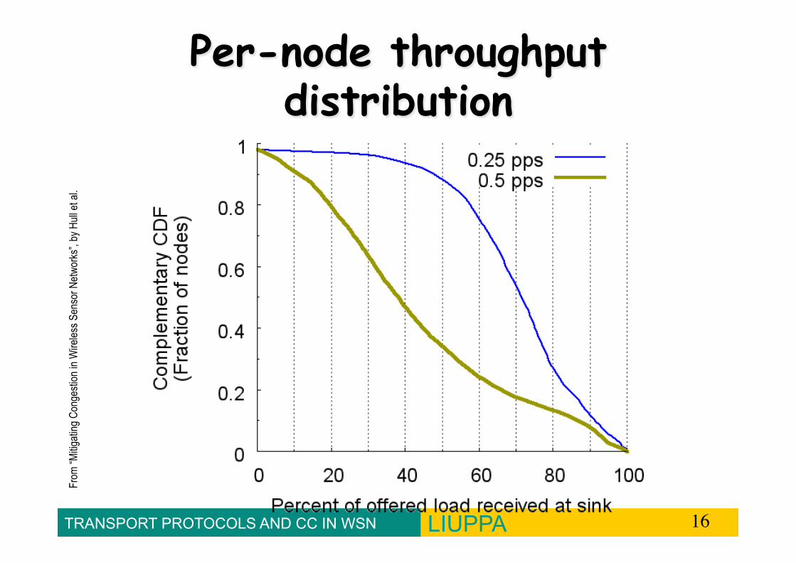
TRANSPORT PROTOCOLS AND CC IN WSN LIUPPA 16
Per-node throughput distribution
From
“Mitig
ating
Con
gesti
on in
Wire
less S
enso
r Netw
orks
”, by
Hull
et al
.

TRANSPORT PROTOCOLS AND CC IN WSN LIUPPA 17
Per-node throughput distribution
From
“Mitig
ating
Con
gesti
on in
Wire
less S
enso
r Netw
orks
”, by
Hull
et al
.
TRANSPORT PROTOCOLS AND CC IN WSN LIUPPA 18
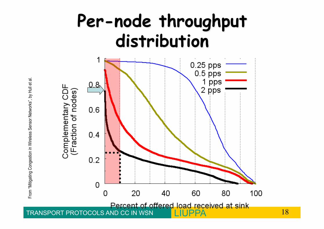
Per-node throughput distribution
From
“Mitig
ating
Con
gesti
on in
Wire
less S
enso
r Netw
orks
”, by
Hull
et al
.

TRANSPORT PROTOCOLS AND CC IN WSN LIUPPA 19
Detecting congestion?
Queue occupancy-based congestion detection Each node has an
output packet queue Monitor
instantaneous output queue occupancy
If queue occupancy exceeds α, indicate local congestion

TRANSPORT PROTOCOLS AND CC IN WSN LIUPPA 20
Queue occupancy not enough!
Channel sampling: sample channel at appropriate time to detect congestion
Report Rate from sources: Fidelity measurement – observed over a long period
C.-Y. Wan, S. B. Eisenman, and A. T. Campbell, “CODA: Congestion detection and avoidance in sensor networks,” in Proceedings of ACM Sensys’03

TRANSPORT PROTOCOLS AND CC IN WSN LIUPPA 21
Channel sampling
Channel status (busy/idle) measured for N consecutive sensing epochs of length E with a predefined sampling rate Φn : # of busy(idle) / epoch
Φn+1=α Φn+(1-α) Φn (EWMA) Experimental validation for
N ∈ {2,3,4,5} E ∈ {100ms, 200ms, 300ms} α ∈ {0.75, 0.80, 0.85, 0.95}

How to upgrade the Internet for QoS?
Approach: de-couple end-system evolution from network evolution
End-to-end protocols: RTP, H.323, etc to spur the growth of adaptive multimedia applications Assume best-effort or better-than-best-effort clouds
Network protocols: IntServ, DiffServ, RSVP, MPLS, COPS … To support better-than-best-effort capabilities at the
network (IP) level

Principles for QOS Guarantees
Consider a phone application at 1Mbps and an FTP application sharing a 1.5 Mbps link. bursts of FTP can congest the router and cause audio packets
to be dropped. want to give priority to audio over FTP
PRINCIPLE 1: Marking of packets is needed for router to distinguish between different classes; and new router policy to treat packets accordingly

Principles for QOS Guarantees (more)
Applications misbehave (audio sends packets at a rate higher than 1Mbps assumed above);
PRINCIPLE 2: provide protection (isolation) for one class from other classes
Require Policing Mechanisms to ensure sources adhere to bandwidth requirements; Marking and Policing need to be done at the edges:

Principles for QOS Guarantees (more)
Alternative to Marking and Policing: allocate a set portion of bandwidth to each application flow; can lead to inefficient use of bandwidth if one of the flows does not use its allocation
PRINCIPLE 3: While providing isolation, it is desirable to use resources as efficiently as possible

Principles for QOS Guarantees (more)
Cannot support traffic beyond link capacity PRINCIPLE 4: Need a Call Admission Process; application
flow declares its needs, network may block call if it cannot satisfy the needs

Summary

High Performance Routers
©cisco
©Juniper
©Procket Networks
©Nortel Networks
©Alcatel ©Lucent
and more…

Generic router architecture
Lookup IP Address
Update Header
Header Processing
Address Table
Lookup IP Address
Update Header
Header Processing
Address Table
Lookup IP Address
Update Header
Header Processing
Address Table
Data Hdr
Data Hdr
Data Hdr
Buffer Manager
Buffer Memory
Buffer Manager
Buffer Memory
Buffer Manager
Buffer Memory
Data Hdr
Data Hdr
Data Hdr

Fundamental Queueing Problems
In a FIFO service discipline, the performance assigned to one flow is convoluted with the arrivals of packets from all other flows! Cant get QoS with a “free-for-all” Need to use new scheduling disciplines which provide “isolation” of performance from arrival rates of background traffic
B
Scheduling Discipline FIFO
B

Queuing Disciplines
Each router must implement some queuing discipline
Queuing allocates bandwidth and buffer space: Bandwidth: which packet to serve next (scheduling) Buffer space: which packet to drop next (buff mgmt)
Queuing also affects latency
Class C
Class B Class A
Traffic Classes
Traffic Sources
Drop Scheduling Buffer Management

Typical Internet Queuing
FIFO + drop-tail Simplest choice Used widely in the Internet
FIFO (first-in-first-out) Implies single class of traffic
Drop-tail Arriving packets get dropped when queue is full
regardless of flow or importance Important distinction:
FIFO: scheduling discipline Drop-tail: drop (buffer management) policy

FIFO + Drop-tail Problems FIFO Issues: In a FIFO discipline, the service seen by a flow is
convoluted with the arrivals of packets from all other flows! No isolation between flows: full burden on e2e control No policing: send more packets get more service
Drop-tail issues: Routers are forced to have have large queues to maintain high utilizations Larger buffers => larger steady state queues/delays Synchronization: end hosts react to same events because packets tend to be
lost in bursts Lock-out: a side effect of burstiness and synchronization is that a few flows
can monopolize queue space

Design Objectives
Keep throughput high and delay low (i.e. knee) Accommodate bursts Queue size should reflect ability to accept bursts
rather than steady-state queuing Improve TCP performance with minimal hardware
changes

Queue Management Ideas
Synchronization, lock-out: Random drop: drop a randomly chosen packet Drop front: drop packet from head of queue
High steady-state queuing vs burstiness: Early drop: Drop packets before queue full Do not drop packets “too early” because queue may reflect only
burstiness and not true overload Misbehaving vs Fragile flows:
Drop packets proportional to queue occupancy of flow Try to protect fragile flows from packet loss (eg: color them or classify
them on the fly) Drop packets vs Mark packets:
Dropping packets interacts w/ reliability mechanisms Mark packets: need to trust end-systems to respond!

Packet Drop Dimensions
Aggregation Per-connection state Single class
Drop position Head Tail
Random location
Class-based queuing
Early drop Overflow drop

Random Early Detection (RED)
Min thresh Max thresh
Average Queue Length
minth maxth
maxP
1.0
Avg queue length
P(drop)
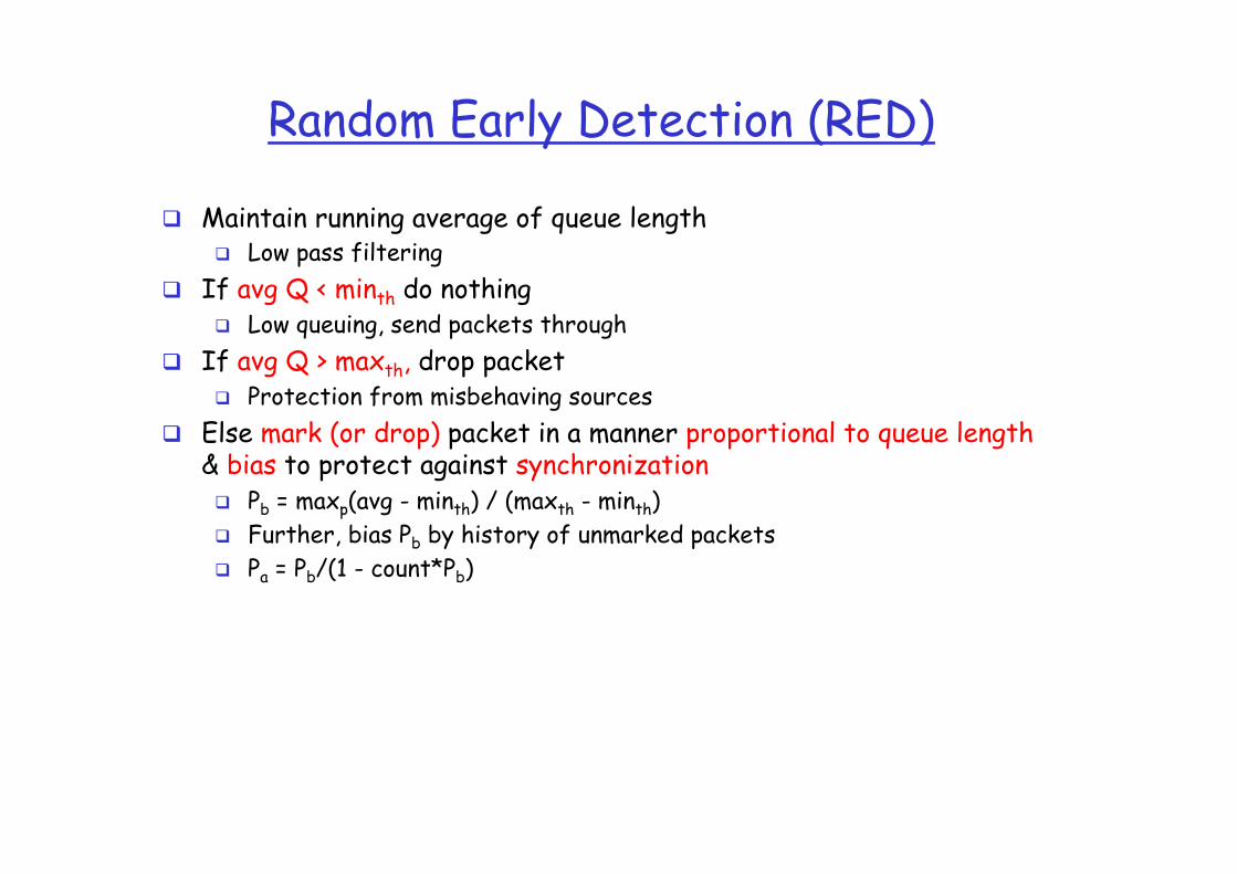
Random Early Detection (RED)
Maintain running average of queue length Low pass filtering
If avg Q < minth do nothing Low queuing, send packets through
If avg Q > maxth, drop packet Protection from misbehaving sources
Else mark (or drop) packet in a manner proportional to queue length & bias to protect against synchronization Pb = maxp(avg - minth) / (maxth - minth) Further, bias Pb by history of unmarked packets Pa = Pb/(1 - count*Pb)
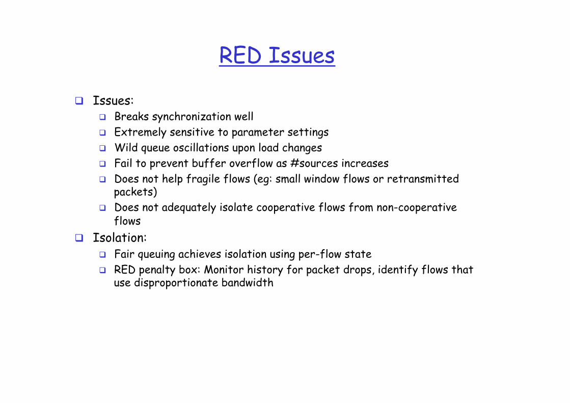
RED Issues
Issues: Breaks synchronization well Extremely sensitive to parameter settings Wild queue oscillations upon load changes Fail to prevent buffer overflow as #sources increases Does not help fragile flows (eg: small window flows or retransmitted
packets) Does not adequately isolate cooperative flows from non-cooperative
flows Isolation:
Fair queuing achieves isolation using per-flow state RED penalty box: Monitor history for packet drops, identify flows that
use disproportionate bandwidth

RED with Multiple Thresholds
Discard Probability
Average Queue Length 0
1
“Red” Threshold
0 “Yellow” Threshold
“Green” Threshold
“Red” Packets
“Green” Packets
“Yellow” Packets
Full
source Juha Heinänen

0 2 4 6 8 10 12 14 16 18 200
0.1
0.2
0.3
0.4
0.5
0.6
0.7
0.8
0.9
1
Link congestion measure
Link marking probability
REM Athuraliya & Low 2000
Main ideas Decouple congestion & performance measure “Price” adjusted to match rate and clear buffer Marking probability exponential in `price’
REM RED
Avg queue
1
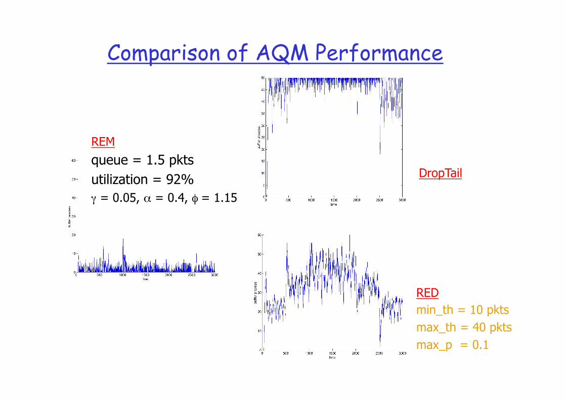
Comparison of AQM Performance
DropTail queue = 94%
RED min_th = 10 pkts max_th = 40 pkts max_p = 0.1
REM
queue = 1.5 pkts utilization = 92% γ = 0.05, α = 0.4, φ = 1.15
SCHEDULING
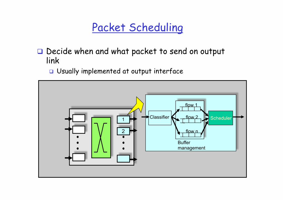
Packet Scheduling
Decide when and what packet to send on output link Usually implemented at output interface
1
2
Scheduler
flow 1
flow 2
flow n
Classifier
Buffer management

Mechanisms: Queuing/Scheduling
Use a few bits in header to indicate which queue (class) a packet goes into (also branded as CoS)
High $$ users classified into high priority queues, which also may be less populated => lower delay and low likelihood of packet drop
Ideas: priority, round-robin, classification, aggregation, ...
Class C
Class B Class A
Traffic Classes
Traffic Sources
$$$$$$
$$$
$

Scheduling And Policing Mechanisms
Scheduling: choosing the next packet for transmission on a link can be done following a number of policies;
FIFO: in order of arrival to the queue; packets that arrive to a full buffer are either discarded, or a discard policy is used to determine which packet to discard among the arrival and those already queued

Priority Queueing Priority Queuing: classes have different priorities; class may
depend on explicit marking or other header info, eg IP source or destination, TCP Port numbers, etc.
Transmit a packet from the highest priority class with a non-empty queue
Preemptive and non-preemptive versions

Round Robin (RR)
Round Robin: scan class queues serving one from each class that has a non-empty queue
one round

Weighted Round Robin (WRR)
Assign a weight to each connection and serve a connection in proportion to its weight
Ex: Connection A, B and C with same packet size and weight
0.5, 0.75 and 1. How many packets from each connection should a round-robin server serve in each round?
Answer: Normalize each weight so that they are all integers: we get 2, 3 and 4. Then in each round of service, the server serves 2 packets from A, 3 from B and 4 from C.
one round
w1
w2
wi

(Weighted) Round-Robin Discussion
Advantages: protection among flows Misbehaving flows will not affect the performance of well-
behaving flows Misbehaving flow – a flow that does not implement any congestion
control FIFO does not have such a property
Disadvantages: More complex than FIFO: per flow queue/state Biased toward large packets (not ATM)– a flow receives service
proportional to the number of packets If packet size are different, we normalize the weight by the
packet size ex: 50, 500 & 1500 bytes with weight 0.5, 0.75 & 1.0

Generalized Processor Sharing (GPS)
Assume a fluid model of traffic Visit each non-empty queue in turn (like RR) Serve infinitesimal from each Leads to “max-min” fairness
GPS is un-implementable! We cannot serve infinitesimals, only packets
max-min fairness
Consider n sources 1,..,n requesting resources x1,..,xn with x1<x2..<xn for instance. Link or server capacity is C.
We assign C/n to source 1. If C/n>x1, we give C/n+(C/n-x1)/(n-1) to the remaining (n-1) sources. If this amount is greater than x2, we iterate.

Packet Approximation of Fluid System
GPS un-implementable Standard techniques of approximating fluid GPS
Select packet that finishes first in GPS assuming that there are no future arrivals (emulate GPS on the side)
Important properties of GPS Finishing order of packets currently in system
independent of future arrivals Implementation based on virtual time
Assign virtual finish time to each packet upon arrival Packets served in increasing order of virtual times
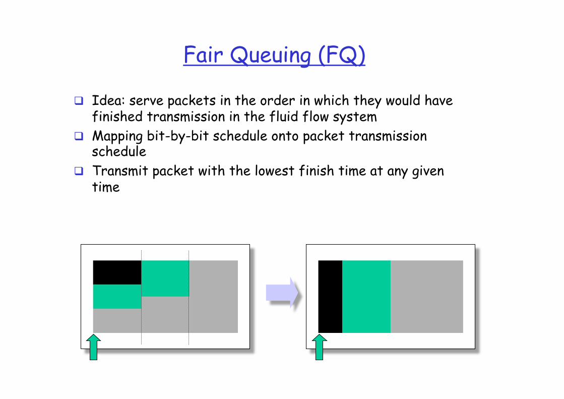
Fair Queuing (FQ)
Idea: serve packets in the order in which they would have finished transmission in the fluid flow system
Mapping bit-by-bit schedule onto packet transmission schedule
Transmit packet with the lowest finish time at any given time

Weighted Fair Queueing
Variation of FQ: Weighted Fair Queuing (WFQ) Weighted Fair Queuing: is a generalized Round
Robin in which an attempt is made to provide a class with a differentiated amount of service over a given period of time

Implementing WFQ
WFQ needs per-connection (or per-aggregate) scheduler state→implementation complexity. complex iterated deletion algorithm complex sorting at the output queue on the service tag
WFQ needs to know the weight assigned for each queue →manual configuration, signalling.
WFQ is not perfect… Router manufacturers have implemented as early
as 1996 WFQ in their products from CISCO 1600 series Fore System ATM switches

Big Picture FQ does not eliminate congestion it just manages
the congestion You need both end-host congestion control and router
support for congestion control end-host congestion control to adapt router congestion control to protect/isolate
Don’t forget buffer management: you still need to drop in case of congestion. Which packet’s would you drop in FQ? one possibility: packet from the longest queue

QOS SPECIFICATION, TRAFFIC, SERVICE
CHARACTERIZATION, BASIC MECHANISMS

Service Specification
Loss: probability that a flow’s packet is lost Delay: time it takes a packet’s flow to get from
source to destination Delay jitter: maximum difference between the
delays experienced by two packets of the flow Bandwidth: maximum rate at which the soource
can send traffic QoS spectrum:
Best Effort Leased Line

Hard Real Time: Guaranteed Services
Service contract Network to client: guarantee a deterministic upper bound
on delay for each packet in a session Client to network: the session does not send more than it
specifies Algorithm support
Admission control based on worst-case analysis Per flow classification/scheduling at routers
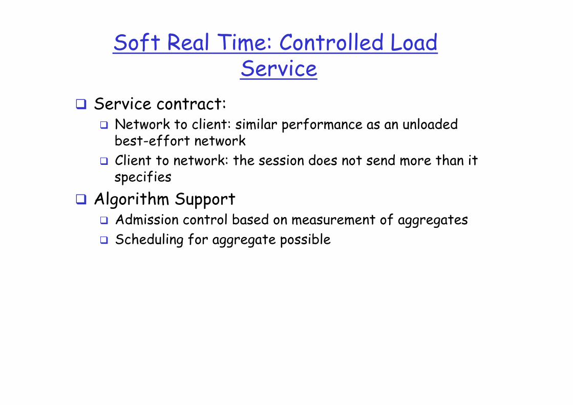
Soft Real Time: Controlled Load Service
Service contract: Network to client: similar performance as an unloaded
best-effort network Client to network: the session does not send more than it
specifies Algorithm Support
Admission control based on measurement of aggregates Scheduling for aggregate possible

Traffic and Service Characterization
To quantify a service one has two know Flow’s traffic arrival Service provided by the router, i.e., resources reserved
at each router Examples:
Traffic characterization: token bucket Service provided by router: fix rate and fix buffer space
Characterized by a service model (service curve framework)

Ex: Token Bucket
Characterized by three parameters (b, R, C) b – token depth R – average arrival rate C – maximum arrival rate (e.g., link capacity)
A bit is transmitted only when there is an available token When a bit is transmitted exactly one token is consumed
R tokens per second
b tokens
<= C bps regulator
time
bits
b*C/(C-R)
slope C
slope R

Token Bucket

Token Bucket

Traffic Envelope (Arrival Curve)
Maximum amount of service that a flow can send during an interval of time t
slope = max average rate b(t) = Envelope
slope = peak rate
t
“Burstiness Constraint”

Arrival curve

Characterizing a Source by Token Bucket
Arrival curve – maximum amount of bits transmitted by time t
Use token bucket to bound the arrival curve
time
bits
Arrival curve
time
bps

Per-hop Reservation with Token Bucket
Given b,r,R and per-hop delay d Allocate bandwidth ra and buffer space Ba such
that to guarantee d
bits
b
slope r Arrival curve
d
Ba
slope ra

What is a Service Model?
The QoS measures (delay,throughput, loss, cost) depend on offered traffic, and possibly other external processes.
A service model attempts to characterize the relationship between offered traffic, delivered traffic, and possibly other external processes.
“external process” Network element
offered traffic delivered traffic
(connection oriented)

Arrival and Departure Process
Network Element Rin Rout
Rin(t) = arrival process = amount of data arriving up to time t
Rout(t) = departure process = amount of data departing up to time t
bits
t
delay
buffer
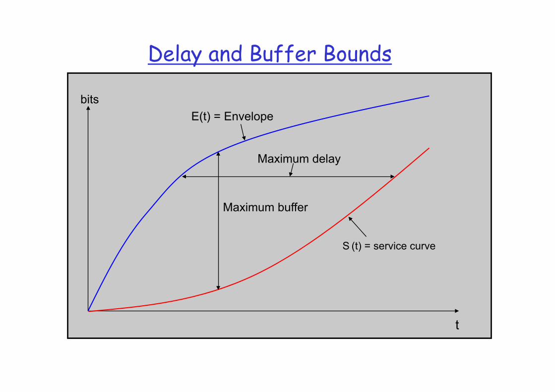
Delay and Buffer Bounds
t
S (t) = service curve
E(t) = Envelope
Maximum delay
Maximum buffer
bits
QoS ARCHITECTURES

Stateless vs. Stateful QoS Solutions
Stateless solutions – routers maintain no fine grained state about traffic scalable, robust weak services
Stateful solutions – routers maintain per-flow state powerful services
guaranteed services + high resource utilization fine grained differentiation protection
much less scalable and robust

Integrated Services (IntServ) An architecture for providing QOS guarantees in IP networks
for individual application sessions Relies on resource reservation, and routers need to maintain
state information of allocated resources (eg: g) and respond to new Call setup requests