fundamentals of traﬃc flow - arxivfundamentals of traﬃc flow dirk helbing ii. institute of...

arX

iv:c

ond-

mat

/980

6080

v1 [

cond

-mat

.sta

t-m

ech]

5 J

un 1

998

Fundamentals of Traffic Flow

Dirk Helbing

II. Institute of Theoretical Physics, University of Stuttgart, Pfaffenwaldring 57/III, 70550

Stuttgart, Germany

Abstract

From single vehicle data a number of new empirical results concerning the

density-dependence of the velocity distribution and its moments as well as the

characteristics of their temporal fluctuations have been determined. These are

utilized for the specification of some fundamental relations of traffic flow and

compared with existing traffic theories.

89.40.+k,47.20.-k,47.50.+d,47.55.-t

Typeset using REVTEX

1

http://arXiv.org/abs/cond-mat/9806080v1

D. Helbing: Fundamentals of traffic flow, PRE 2

For the prosperity in industrialized countries, efficient traffic systems are indispensable.

However, due to an overall increase of mobility and transportation during the last years, the

capacity of the road infrastructure has been reached. Some cities like Los Angeles and San

Francisco already suffer from daily traffic collapses and their environmental consequences.

About 20 percent more fuel consumption and air pollution is caused by impeded traffic and

stop-and-go traffic.

For the above mentioned reasons, several models for freeway traffic have been proposed,

microscopic and macroscopic ones (for an overview cf. Ref. [1]). These are used for devel-

oping traffic optimization measures like on-ramp control, variable speed limits or re-routing

systems [1]. For such purposes, the best models must be selected and calibrated to empirical

traffic relations. However, some relations are difficult to obtain, and the lack of available

empirical data has caused some stagnation in traffic modeling.

Further advances will require a close interplay between theoretical and empirical inves-

tigations [2]. On the one hand, empirical findings are necessary to test and calibrate the

various traffic models. On the other hand, some hardly measurable quantities and relations

can be reconstructed by means of theoretical relations.

Therefore, a number of fundamental traffic relations will be presented in the following.

Until now, little is known about the velocity distribution of vehicles, its variance or skewness.

A similar thing holds for the functional form of the velocity-density relation or the variance-

density relation at high densities. Empirical results have also been missing for the fluctuation

characteristics of the density or average velocity. These gaps will be closed in the following.

Although the data are varying in detail from one freeway stretch to another, the essential

conclusions are expected to be universal.

In a recent paper [3] it has been shown that the traffic dynamics on neighboring lanes

is strongly correlated. Therefore, it is possible to treat the total freeway cross section in

an overall way. Consequently, we will only discuss the properties of the lane averages of

macroscopic traffic quantities. The empirical relations have been evaluated from single

vehicle data of the Dutch two-lane freeway A9 between Haarlem and Amsterdam (for a


sketch cf. Fig. 1 in Ref. [3]). These data were detected by induction loops at discrete places

x of the roadway and include the passage times tα(x), velocities vα(x), and lengths lα(x)

of the single vehicles α. Consequently, it was possible to calculate the number N(x, t) of

vehicles which passed the cross section at place x during a time interval [t − T/2, t + T/2],

the traffic flow

Q(x, t) := N(x, t)/T , (1)

and the macroscopic velocity moments

〈vk〉 :=1

N(x, t)

∑

t−T/2≤tα(x)<t+T/2

[vα(x)]k . (2)

Small values of T are connected with large statistical variations of the data, but large values

can cause biased results for k ≥ 2 [3]. Values between 0.5 and 2 minutes seem to be the

best compromise [1]. The vehicle densities ρ(x, t) were calculated via the theoretical flow

formula

Q(x, t) = ρ(x, t)V (x, t) . (3)

Other evaluation methods [4] are discussed in Ref. [1].

We start with the discussion of the grouped empirical velocity distribution P (v; x, t)

which was obtained in the usual way:

P (vl; x, t) :=n(x, vl, t)

N(x, t). (4)

Here, n(x, vl, t) denotes the number of vehicles which pass the cross section at x between

times t−T/2 and t+T/2 with a velocity v ∈ [vl −∆/2, vl +∆/2). The class interval length

was chosen ∆ = 5km/h.

In theoretical investigations, the velocity distribution P (v; x, t) has mostly been assumed

to have the Gaussian form [5–7]

PG(v; x, t) :=1

√

2πΘ(x, t)exp

(

− [v − V (x, t)]2

2Θ(x, t)

)

. (5)


Here, V (x, t) := 〈v〉 denotes the average velocity and Θ(x, t) := 〈[v − V (x, t)]2〉 the velocity

variance. Assumption (5) has been made for two reasons: First, it allows to derive approx-

imate fluid-dynamic traffic equations from a gas-kinetic level of description [5–7]. Second,

analytical results for the velocity distribution are not yet available, even for the stationary

and spatially homogeneous case. Therefore the question is, whether the Gaussian approxi-

mation is justified or not. Figure 1 gives a positive answer, at least for the average velocity

distribution at small and medium densities. In particular, bimodal distributions are not

observed [8].

An investigation of the temporal evolution of the velocity distribution is difficult due

to the large statistical fluctuations (which come from the fact that only a few vehicles

per velocity class pass the observed freeway cross section during the short time period T ).

Therefore, we will study a macroscopic (aggregated) quantity instead, namely the temporal

variation of the skewness

γ(x, t) :=〈[v − V (x, t)]3〉

[Θ(x, t)]3/2=

〈v3〉 − 3〈v〉〈v2〉 + 2〈v〉3[Θ(x, t)]3/2

. (6)

This can be interpreted as a dimensionless measure of asymmetry (cf. Fig. 2). Figure 3

shows that the skewness mainly varies between −0.5 and 0.5. The deviation from 0 is neither

systematic nor significant, so that the skewness is normally negligible. This indicates that

even the time-dependent velocity distribution is approximately Gaussian-shaped [9].

Now it will be investigated how the average velocity V and the variance Θ depend on the

vehicle density ρ (cf. Figs. 4 and 5). The problem is that the data for high vehicle densities

are missing. However, for computer simulations of the traffic dynamics the corresponding

functional relations need to be specified. This can be done by means of theoretical results.

For the average velocity and variance on freeways with speed limits, recent gas-kinetic traffic

models [6] imply the following implicit equilibrium relations (indicated by a subscript “e”),

if the skewness is neglected (cf. Fig. 3):

Ve(ρ) = V0 −τ(ρ)[1 − p(ρ)]ρΘe(ρ)

1 − ρ/ρmax − ρTrVe(ρ), (7)


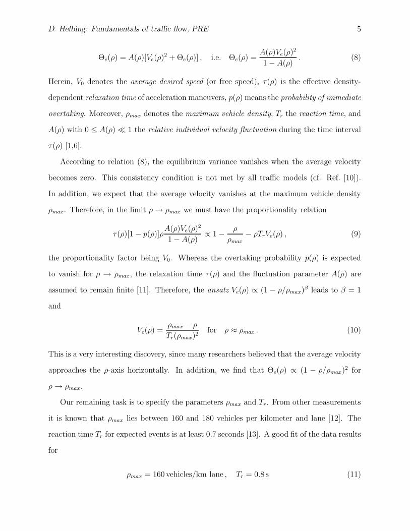
Θe(ρ) = A(ρ)[Ve(ρ)2 + Θe(ρ)] , i.e. Θe(ρ) =A(ρ)Ve(ρ)2

1 − A(ρ). (8)

Herein, V0 denotes the average desired speed (or free speed), τ(ρ) is the effective density-

dependent relaxation time of acceleration maneuvers, p(ρ) means the probability of immediate

overtaking. Moreover, ρmax denotes the maximum vehicle density, Tr the reaction time, and

A(ρ) with 0 ≤ A(ρ) ≪ 1 the relative individual velocity fluctuation during the time interval

τ(ρ) [1,6].

According to relation (8), the equilibrium variance vanishes when the average velocity

becomes zero. This consistency condition is not met by all traffic models (cf. Ref. [10]).

In addition, we expect that the average velocity vanishes at the maximum vehicle density

ρmax. Therefore, in the limit ρ → ρmax we must have the proportionality relation

τ(ρ)[1 − p(ρ)]ρA(ρ)Ve(ρ)2

1 − A(ρ)∝ 1 − ρ

ρmax− ρTrVe(ρ) , (9)

the proportionality factor being V0. Whereas the overtaking probability p(ρ) is expected

to vanish for ρ → ρmax, the relaxation time τ(ρ) and the fluctuation parameter A(ρ) are

assumed to remain finite [11]. Therefore, the ansatz Ve(ρ) ∝ (1 − ρ/ρmax)β leads to β = 1

and

Ve(ρ) =ρmax − ρ

Tr(ρmax)2for ρ ≈ ρmax . (10)

This is a very interesting discovery, since many researchers believed that the average velocity

approaches the ρ-axis horizontally. In addition, we find that Θe(ρ) ∝ (1 − ρ/ρmax)2 for

ρ → ρmax.

Our remaining task is to specify the parameters ρmax and Tr. From other measurements

it is known that ρmax lies between 160 and 180 vehicles per kilometer and lane [12]. The

reaction time Tr for expected events is at least 0.7 seconds [13]. A good fit of the data results

for

ρmax = 160 vehicles/km lane , Tr = 0.8 s (11)


(cf. Fig. 4). In addition we can conclude from (7) that the velocity-density relation Ve(ρ)

of a multi-lane freeway should start horizontally, since the probability of overtaking p(ρ)

should approach the value 1 at very small densities ρ ≈ 0.

However, it is not only possible to reconstruct the functional forms of the velocity-density

relation Ve(ρ) and the variance-density relation Θe(ρ). From these we can also determine

the dependence of the model functions A(ρ) and τ(ρ)[1 − p(ρ)] by means of the theoretical

relations (7) and (8). The result for the diffusion strength A(ρ) is depicted in Figure 6.

Finally, we will investigate the temporal fluctuations of the empirical vehicle density

ρ(x, t). Until now, most related studies have been presented theoretical or simulation results.

It has been claimed that the power spectrum ρ(x, ν) of the density ρ(x, t) obeys a power law

ρ(x, ν) ∝ ν−δ , i.e. log ρ(x, ν) = C − δ log ν . (12)

For δ, the values 1.4 [14], 1.0 [15], or 1.8 [16] have been found. The empirical results in

Figure 7 indicate that the exponent δ is 2.0 at small frequencies ν, otherwise 0.0. Taking

into account the logarithmic frequency scale, we can conclude that the power spectrum is

flat for the most part of the frequency range. This corresponds to a white noise. Analogous

results are found for the power spectrum of the average velocity V (x, t) [1].

In summary, we found that the velocity distribution is approximately Gaussian dis-

tributed and that its skewness is negligible. We were able to reconstruct the velocity-density

relation Ve(ρ) and the variance-density relation Θe(ρ) by means of theoretical results. This

allowed the determination of some density-dependent model parameters. The fluctuations

of the vehicle density could be approximated by a white noise, although a power law with

exponent 2.0 was found at small frequencies. All these results are necessary for realistic

traffic simulations.

ACKNOWLEDGMENTS

The author is grateful to Henk Taale and the Ministry of Transport, Public Works and

Water Management for supplying the freeway data.


REFERENCES

[1] D. Helbing, Verkehrsdynamik. Neue physikalische Modellierungskonzepte (Springer,

Berlin, in preparation).

[2] B. S. Kerner and H. Rehborn, Phys. Rev. E 53, 1297 and 4275 (1996).

[3] D. Helbing, Empirical traffic data and their implications for traffic modeling, submitted

to Phys. Rev. E (1996).

[4] For example, averaging over a small stretch of length X between x−X/2 and x + X/2

at time t instead of averaging over a time inteval T at place x will not exactly lead to

the same results [1]. However, the difference in the velocity moments is of order Θ/V 2

and therefore negligible.

[5] D. Helbing, Phys. Rev. E 53, 2366 (1996).

[6] D. Helbing, Derivation and empirical validation of a refined traffic flow model, Physica

A, in print (1996).

[7] C. Wagner et al., Second order continuum traffic flow model, Phys. Rev. E, submitted

(1996).

[8] Publications by W. F. Phillips [Transportation Planning and Technology 5, 131 (1979)]

and by R. D. Kuhne [in Proceedings of the 9th International Symposium on Trans-

portation and Traffic Theory, edited by I. Volmuller and R. Hamerslag (VNU Science,

Utrecht, 1984)] have reported about bimodal distributions at large vehicle densities.

However, the reason seems to be that they chose a large time interval T . Consequently,

fast changes of the traffic conditions like stop-and-go waves could produce a velocity

distribution that appears bimodal.

[9] An exact proof of this conclusion would require a comparison of all higher empirical

velocity moments with the corresponding relations for a Gaussian distribution. However,


for many theoretical considerations it is sufficient to know that the skewness vanishes

and that the velocity distribution is unimodal.

[10] D. Helbing, Phys. Rev. E 51, 3164 (1995).

[11] This is supported by empirical observations. If τ(ρ) would diverge for ρ → ρmax, a traffic

jam would not be able to dissolve, once is came to rest. Moreover, vehicles always keep

some minimal distance from each other, so that ρmax is smaller than the reciprocal 1/l

of the average vehicle length l. This guarantees the possibility to move.

[12] R. Kuhne, in Highway Capacity and Level of Service, edited by U. Brannolte (Balkema,

Rotterdam, 1991) and unpublished material.

[13] A. D. May, Traffic Flow Fundamentals (Prentice Hall, Englewood Cliffs, NJ, 1990).

[14] T. Musha and H. Higuchi, Japanese Journal of Applied Physics 17, 811 (1978).

[15] K. Nagel and H. J. Herrmann, Physica A 199, 254 (1993); K. Nagel and M. Paczuski,

Phys. Rev. E 51, 2909 (1995); X. Zhang and G. Hu, Phys. Rev. E 52, 4664 (1995); M.

Y. Choi and H. Y. Lee, Phys. Rev. E 52, 5979 (1995).

[16] S. Yukawa and M. Kikuchi, Journal of the Physical Society of Japan 65, 916 (1996).


FIGURES

0

0.1

0.2

0.3

0.4

0.5

0.6

0.7

0.8

0.9

1

0 20 40 60 80 100 120 140

v (km/h)

P(v

;r,t

)ρ = 90vehicles/km lane

80

70

60

50 40 30 2010

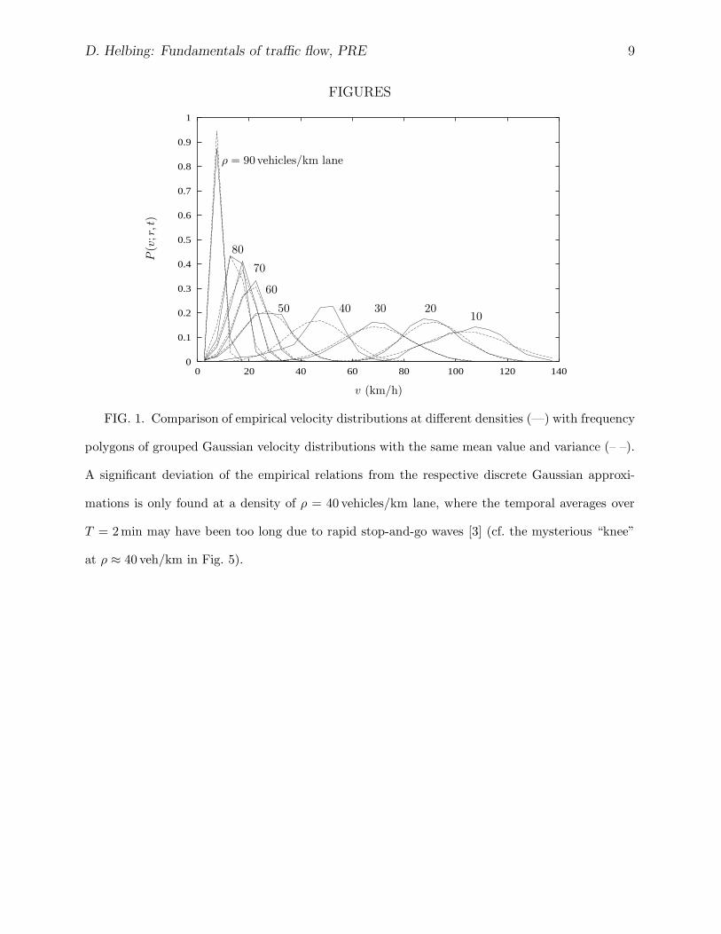
FIG. 1. Comparison of empirical velocity distributions at different densities (—) with frequency

polygons of grouped Gaussian velocity distributions with the same mean value and variance (– –).

A significant deviation of the empirical relations from the respective discrete Gaussian approxi-

mations is only found at a density of ρ = 40 vehicles/km lane, where the temporal averages over

T = 2min may have been too long due to rapid stop-and-go waves [3] (cf. the mysterious “knee”

at ρ ≈ 40 veh/km in Fig. 5).


0

0.1

0.2

0.3

0.4

0.5

0.6

-5 -4 -3 -2 -1 0 1 2 3 4 5(v − V )√

Θ

Pγ(v

)

FIG. 2. Velocity distributions Pγ(v) := {1 − γ[3(v − V )/Θ1/2 − (v − V )3/Θ3/2]/6}PG(v) with

the same average velocity V and variance Θ, but different values of the skewness γ (— : γ = 0;

– – : γ = 1/2; - - - : γ = 1; · · · : γ = 2). Obviously, a skewness of |γ| ≤ 0.5 only leads to minor

changes compared to the Gaussian distribution (—).


-4

-3

-2

-1

0

1

2

3

4

0 20 40 60 80 100 120 140 160

ρ (vehicles/km lane)

γ

FIG. 3. Density-dependence of the skewness γ (· : 1-minute data; 3: respective mean values).

The large variation of the 1-minute data at low densities is due to the small number of vehicles

which pass a cross section during the time interval T = 1min, whereas the large variation of their

mean values at high densities comes from the few 1-minute data, over which could be averaged.

The 1-minute data of the skewness scatter around the zero line (—) and mostly lie between −0.5

and 0.5.


0

20

40

60

80

100

120

140

0 20 40 60 80 100 120 140 160


V(k

m/h)

FIG. 4. Relation between average velocity and density (·: 1-minute data; 3: respective mean

values; —: fit function for the equilibrium relation Ve(ρ)). The speed limit is 120 km/h (– –).

0

5

10

15

20

25

0 20 40 60 80 100 120 140 160


√Θ

(km

/h)

FIG. 5. Density-dependence of the standard deviation√

Θ of the vehicle velocities (·: 1-minute

data; 3: respective mean values; —: fit function for the equilibrium relation√

Θe(ρ)).


0

0.01

0.02

0.03

0.04

0.05

0 20 40 60 80 100 120 140 160


A(ρ

)

FIG. 6. Density-dependence of the fluctuation strength A(ρ), which is a measure for the relative

velocity variation during a time interval τ(ρ). Its maximum at medium densities indicates that

velocity fluctuations are particularly large in the region of unstable traffic flow.

1

2

3

4

5

6

7

8

9

-3 -2.5 -2 -1.5 -1 -0.5 0

log(ν min)

log

ρ(ν

)

FIG. 7. The power spectrum of the time-dependent vehicle density ρ(x, t) follows a power law

with exponent δ = 2.0 at very small frequencies ν, but it is flat over large parts of the frequency

range, corresponding to a white noise.

fundamentals of traﬃc flow - arxivfundamentals of traﬃc flow dirk helbing ii. institute of...

Documents