FUNNEL: Automatic Mining ofSpatially Coevolving Epidemics

Yasuko Matsubara†, Yasushi Sakurai†, Willem G. van Panhuis§, Christos Faloutsos‡

† Dept. of Computer Science and Electrical Engineering, Kumamoto University,§ Dept. of Epidemiology, University of Pittsburgh, ‡ Dept. of Computer Science, Carnegie Mellon University

{yasuko,yasushi}@cs.kumamoto-u.ac.jp, wav10@pitt.edu, christos@cs.cmu.edu

ABSTRACT

Given a large collection of epidemiological data consisting of thecount of d contagious diseases for l locations of duration n, howcan we find patterns, rules and outliers? For example, the ProjectTycho provides open access to the count infections for U.S. statesfrom 1888 to 2013, for 56 contagious diseases (e.g., measles, in-fluenza), which include missing values, possible recording errors,sudden spikes (or dives) of infections, etc. So how can we find acombined model, for all these diseases, locations, and time-ticks?

In this paper, we present FUNNEL, a unifying analytical modelfor large scale epidemiological data, as well as a novel fitting algo-rithm, FUNNELFIT, which solves the above problem. Our methodhas the following properties: (a) Sense-making: it detects impor-tant patterns of epidemics, such as periodicities, the appearance ofvaccines, external shock events, and more; (b) Parameter-free: ourmodeling framework frees the user from providing parameter val-ues; (c) Scalable: FUNNELFIT is carefully designed to be linearon the input size; (d) General: our model is general and practi-cal, which can be applied to various types of epidemics, includingcomputer-virus propagation, as well as human diseases.

Extensive experiments on real data demonstrate that FUNNELFIT

does indeed discover important properties of epidemics: (P1) dis-ease seasonality, e.g., influenza spikes in January, Lyme diseasespikes in July and the absence of yearly periodicity for gonorrhea;(P2) disease reduction effect, e.g., the appearance of vaccines; (P3)local/state-level sensitivity, e.g., many measles cases in NY; (P4)external shock events, e.g., historical flu pandemics; (P5) detectincongruous values, i.e., data reporting errors.

Categories and Subject Descriptors: H.2.8 [Database manage-

ment]: Database applications–Data mining

Keywords: Epidemics; Time-series; Automatic mining

1. INTRODUCTIONGiven a huge collection of co-evolving epidemic time-series,

such as measles and influenza, how can we find typical patterns oranomalies, and statistically summarize all the epidemic sequences?In this paper, we present a unifying model, namely FUNNEL, which

Permission to make digital or hard copies of all or part of this work for personal or

classroom use is granted without fee provided that copies are not made or distributed

for profit or commercial advantage and that copies bear this notice and the full cita-

tion on the first page. Copyrights for components of this work owned by others than

ACM must be honored. Abstracting with credit is permitted. To copy otherwise, or re-

publish, to post on servers or to redistribute to lists, requires prior specific permission

and/or a fee. Request permissions from permissions@acm.org.

KDD’14, August 24–27, 2014, New York, NY, USA.

Copyright 2014 ACM 978-1-4503-2956-9/14/08 ...$15.00.

http://dx.doi.org/10.1145/2623330.2623624.

provides a good description of large collections of epidemiologicaldata. 1 Intuitively, the problem we wish to solve is as follows:

INFORMAL PROBLEM 1. Given a large collection of epidemi-

ological data, which consists of d diseases in l locations of duration

n, with missing values and recording errors, we want to

• find basic patterns of diseases (e.g., seasonality)

• find extra patterns (e.g., outbreaks, sudden drops)

• detect anomalies (i.e., possible errors)

Uncovering the mechanisms and patterns of contagious diseasesis an important and challenging task for public health scientists andpolicy makers. In this paper, we study a publicly available resourceof epidemiological data: Tycho [32], which contains the count ofinfections of 56 diseases in the U.S, covering over 125 years on aweekly basis. 2

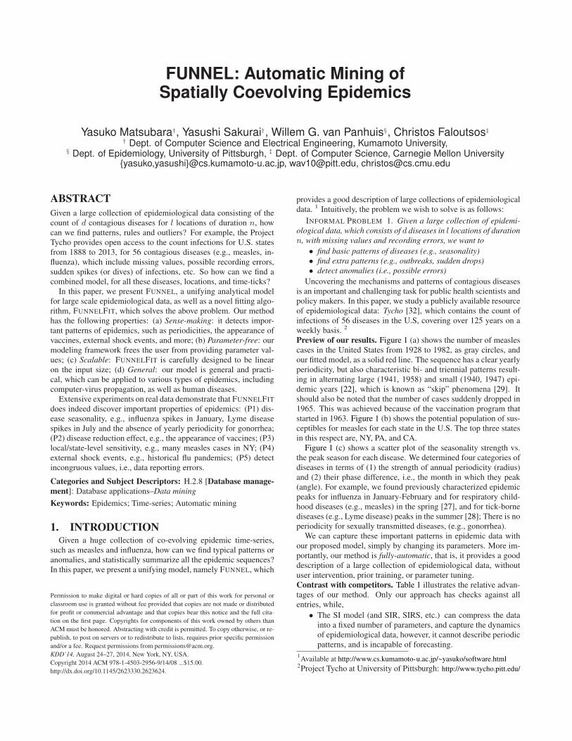
Preview of our results. Figure 1 (a) shows the number of measlescases in the United States from 1928 to 1982, as gray circles, andour fitted model, as a solid red line. The sequence has a clear yearlyperiodicity, but also characteristic bi- and triennial patterns result-ing in alternating large (1941, 1958) and small (1940, 1947) epi-demic years [22], which is known as “skip” phenomena [29]. Itshould also be noted that the number of cases suddenly dropped in1965. This was achieved because of the vaccination program thatstarted in 1963. Figure 1 (b) shows the potential population of sus-ceptibles for measles for each state in the U.S. The top three statesin this respect are, NY, PA, and CA.

Figure 1 (c) shows a scatter plot of the seasonality strength vs.the peak season for each disease. We determined four categories ofdiseases in terms of (1) the strength of annual periodicity (radius)and (2) their phase difference, i.e., the month in which they peak(angle). For example, we found previously characterized epidemicpeaks for influenza in January-February and for respiratory child-hood diseases (e.g., measles) in the spring [27], and for tick-bornediseases (e.g., Lyme disease) peaks in the summer [28]; There is noperiodicity for sexually transmitted diseases, (e.g., gonorrhea).

We can capture these important patterns in epidemic data withour proposed model, simply by changing its parameters. More im-portantly, our method is fully-automatic, that is, it provides a gooddescription of a large collection of epidemiological data, withoutuser intervention, prior training, or parameter tuning.Contrast with competitors. Table 1 illustrates the relative advan-tages of our method. Only our approach has checks against allentries, while,

• The SI model (and SIR, SIRS, etc.) can compress the datainto a fixed number of parameters, and capture the dynamicsof epidemiological data, however, it cannot describe periodicpatterns, and is incapable of forecasting.

1Available at http://www.cs.kumamoto-u.ac.jp/~yasuko/software.html

2Project Tycho at University of Pittsburgh: http://www.tycho.pitt.edu/

1930 1940 1950 1960 1970 19800

2

4

6x 10

4

Year

Cou

nt

1930 1940 1950 1960 1970 1980

105

Year

Cou

nt (

log)

OriginalI(t)

OriginalS(t)I(t)V(t)

Vaccination

(a) Fitting result of FUNNELFIT (measles)

(b) Potential population of susceptibles (measles)

0.1

0.2

0.3

0.4

0.5

February (2)

August (8)

March (3)

September (9)

April (4)

October (10)

May (5)

November (11)

June (6)

December (12)

July (7) January (1)

RubellaMeasles

Mumps

Gonorrhea

Streptococcal sore throat

ChickenpoxSmallpox

Lymedisease

Typhoidfever

Cryptosporidiosis

Rocky mountain spotted fever

Typhus fever

Influenza

(c) Seasonality strength (radius) vs. peak season (angle)

Figure 1: Modeling power of FUNNELFIT: (a) the original number of measles cases (gray dots), and our model (red lines). It

captures the yearly cycle, external spikes, and vaccination starting in 1963, as well as (b) the local sensitivity (e.g., many patients in

NY, PA, CA, TX); (c) the scatter plot of the seasonality strength vs. the peak season - (angle): the peak month for each disease and

(radius): the strength of the fluctuation, e.g., influenza peaks every winter, measles in the spring, and no periodicity for gonorrhea.

Table 1: Capabilities of approaches. Only our approach meets

all specifications.

SIRS AR/PLiF PARAFAC FUNNELFIT

Compression√ √ √ √

Domain knowledge√ √

Missing values√ √

Periodicity√ √

Forecasting√ √

Parameter free√

• The auto regression (AR) model and PLiF [15] have the abil-ity to compress and forecast sequences, but they are funda-mentally unsuitable for epidemic data, and cannot capturethe non-linear patterns of virus propagation.

• Our epidemic data can be turned into a tensor. PARAFAC iscapable of compression, but it cannot handle missing values,periodicity, or forecasting.

Most importantly, none of above are parameter-free methods.Contributions. Our method has the following desirable properties:

1. Sense-making: thanks to our modeling framework, our methodcan provide an intuitive explanation for epidemics, such asthe seasonality of diseases, vaccination, and external shocks.It matches the behavior of various types of contagious dis-eases, such as measles, influenza, and smallpox.

2. Automatic: it is fully automatic, requiring no human inter-vention. Our algorithm is theoretically founded on the ideaof minimizing the cost of the resulting modeling.

3. Scalable: it scales linearly with the input size.4. Generality: it includes earlier patterns and models as special

cases (e.g., SIRS), and it can be applied to various types ofepidemic data including computer virus infections.

Outline. The rest of the paper is organized in the conventionalway: Next we describe related work, followed by our proposedmodel and algorithms, experiments, discussion and conclusions.

2. RELATED WORKWe provide a survey of the related literature, which falls broadly

into two categories: (1) epidemiology, and (2) pattern discovery intime series.

Epidemiology. The canonical textbook for epidemiological mod-els including SI/SIR is Anderson and May [2]. Grenfell et al. [9]studied the recurrent travelling waves for measles, while the workin [8] explained the complex dynamical transitions in epidemics.Stone et al. [29] studied the seasonal dynamics of recurrent epi-demics including measles, and identified a new threshold for pre-dicting the occurrence of either a future epidemic, or a ‘skip’ (i.e., ayear in which an epidemic fails to initiate). Van Panhuis et al. [32]digitized the entire history of weekly Nationally Notifiable DiseaseSurveillance Reports for the U.S. from 1888 to 2013.Pattern discovery in time series. In recent years, there has beenan explosion of interest in mining time series [4, 6, 21, 16]. Tra-ditional approaches applied to data mining include auto-regression(AR), linear dynamical systems (LDS), Kalman filters (KF) andtheir variants [10, 15, 31]. Similarity search and pattern discov-ery in time sequences have also attracted huge interest [33, 13, 30,26, 7]. Regarding large-scale time-series mining, TriMine [18] isa scalable method for forecasting co-evolving multiple (thousandsof) sequences, while, [17] developed a fully-automatic mining al-gorithm for co-evolving time sequences. Rakthanmanon et al. [25]proposed a similarity search algorithm for “trillions of time series”under the DTW distance. Recently, analyses of epidemics, so-cial media, propagation and the cascades they create have attractedmuch interest [24, 12, 14, 23, 19].

However, none of these methods specifically focused on auto-matic mining of non-linear dynamics in coevolving epidemics.

3. PROPOSED MODELIn this section we present our proposed model.

3.1 Design philosophy of FUNNELData description. The Project Tycho [32] covers more than a cen-tury of weekly surveillance reports of nationally notifiable diseases(56 diseases in total) for all 50 states in the U.S, from 1888 to thepresent, with 87,950,807 reported individual cases for diseases.

This dataset consists of tuples of the form: (disease, location,

timestamp). We then have a collection of entries with d uniquediseases, and l states, with duration n (on a weekly basis). We can

40 60 8010

0

105

Temperature (F)

# of

cas

es (

log)

1942 1943 1944 1945 194610

0

105

case

s (lo

g)

1942 1943 1944 1945 19460

50

100

Tem

pera

ture

Year

CATXVA

1931 1932 1933 1934 193510

0

102

104

case

s (lo

g)

20 40 60 80

102

104

Temperature (F)

# of

cas

es (

log)

1931 1932 1933 1934 19350

50

100

Tem

pera

ture

Year

CANYPA

(a) Influenza (in CA, TX, VA) (b) Measles (in CA, NY, PA)

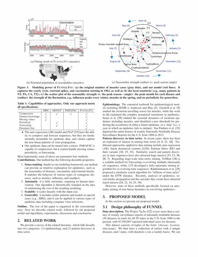
Figure 2: The air temperature vs. # of cases: (a) influenza is

completely anti-correlated with the air temperature (i.e., peak-

ing in the winter), while, (b) measles also has strong periodicity,

but it peaks in the spring (i.e., with a phase shift).

treat this set of d × l epidemic sequences as a 3rd-order tensor,i.e., X ∈ N

d×l×n, where the element xij(t) of X shows the totalnumber of entries of the i-th disease in the j-th state at time-tick t.

For example, (‘measles’, ‘PA’, ‘April 1-7, 1931’; 4740), meansthat the number of cases due to ‘measles’ in ‘PA’ on ‘April 1-7 in1931’ is ‘4740’.

We refer to each sequence of the i-th disease in the j-th state:xij = {xij(t)}

nt=1, as a “local/state”-level epidemic sequence.

Similarly, we can turn these local sequences into “global/country”-level epidemics: x̄i = {x̄i(t)}

nt=1, where x̄i(t) shows the total

count of the i-th disease at time-tick t, i.e., x̄i(t) =∑l

j=1 xij(t).Preliminary observations. Here, we provide the reader with sev-eral important observations. Figure 2 shows the scatter plots (top)and sequence plots (bottom) of the original local-level sequencesof influenza and measles counts in three states, versus the aver-age air temperature for five years. 3 In Figure 2 (a), influenzacases are strongly anti-correlated with the air temperature, corre-sponding to influenza epidemics in colder seasons. On the otherhand, for measles (Figure 2 (b)), the scatter plot exhibits charac-teristic loop shapes, which indicates that there is a phase shift ofmeasles vs. temperature - actually, measles peaks in the spring. Asshown in Figure 1 (c), there are several groups of infectious dis-eases with specific seasonal patterns, including children’s diseases(e.g., measles, mumps) in the spring, and tick-borne diseases (e.g.,Lyme disease) in the summer. Consequently we have:

OBSERVATION 1 (DISEASE SEASONALITY). Many diseases

have yearly cycles with different phases, that is, they are correlated

with air temperature and the seasons.

The next observation refers to the abrupt decline of several dis-eases. Luckily, many diseases have been eradicated or significantlyreduced over the last century, through various factors including vac-cination, sanitation and antibiotics. For example, in Figure 1 (a),the number of measles cases has been decreasing since the vacci-nation program was introduced in 1963. We will collectively referto such abrupt declines as disease reduction effects.

OBSERVATION 2 (DISEASE REDUCTION EFFECT). Many in-

fectious diseases have been reduced or eliminated through vacci-

nation programs, antibiotics, sanitation, etc.

Next, let us look at the topic from a local point of view. InFigure 2, three local sequences are correlated with each other, butwith different fractions of patients, which correspond to the numberof susceptible people in each state. For example, measles mainlyaffects children, and so, the more children there are, the more casesof measles there will be (see, NY, PA, CA, TX, in Figure 1 (b)).

3 National climate data center: http://www.ncdc.noaa.gov/cag/

Table 2: Symbols and definitionsSymbol Definition

d Number of diseasesl Number of states (i.e., locations)n Duration of sequences

X 3rd-order tensor (X ∈ Nd×l×n)

xij Local-level epidemic sequence of disease i in state jx̄i Global-level epidemic sequence of disease i

Sij(t) Count of susceptibles of disease i in state j at time tIij(t) Count of infectives of disease i in state j at time tVij(t) Count of vigilants of disease i in state j at time t

B Base matrix (d× 6) i.e., B = {b1, . . . , bd}R Disease reduction matrix (d× 2) i.e., R = {r1, . . . , rd}N Geo-disease matrix (d× l) i.e., N = {Nij}d,li,j=1

E External shock tensor i.e., E = {E(D), E(T), E(S)}M Mistake tensor i.e., M = {mij(t)}d,l,ni,j,t=1

F Complete set of FUNNEL i.e., F = {B,R,N,E ,M }OBSERVATION 3 (AREA SPECIFICITY AND SENSITIVITY). For

each disease, neighbors are correlated with different sensitivity.

The last two observations are the extra properties of epidemics.Figure 1 (a) shows large outbreaks of measles in 1941 and 1958,while Figure 2 (a) shows two large flu pandemics in 1944 and 1946.

OBSERVATION 4 (EXTERNAL SHOCK EVENTS). There are some

extreme spikes, representing major events such as historical flu

pandemics.

Basically, real-world datasets are subject to quality constraintssuch as typing errors and incorrect reports (we refer to them as“mistakes”).

OBSERVATION 5 (MISTAKES). There are some implausible

spikes, which are completely independent of the dynamics of epi-

demic patterns.

Summary. In this paper, we propose a new model, namely, FUN-NEL, which tries to incorporate all the above important proper-ties that we observed in the real epidemic data. Consequently, wewould like to capture the following properties:

• (P1): yearly periodicity• (P2): disease reduction effects• (P3): area specificity and sensitivity• (P4): external shock events• (P5): mistakes, incorrect values

For simplicity, let’s focus on a simple step first, where (a) we as-sume that we are given a single epidemic sequence, say, the numberof measles cases in NY. We then (b) extend our model to multipleco-evolving epidemics, that is, to capture the individual patterns ofd diseases in l states.

3.2 FUNNEL - with a single epidemicWe begin with the simplest case, where we assume that we are

given a single epidemic sequence.

3.2.1 Base model - FUNNEL-BASE

The model we propose has nodes (=people) of three classes:

• Susceptible: nodes in this class can get infected by any neigh-boring node who is infectious.

• Infected: nodes who have been infected and are capable oftransmitting the infection to those in the susceptible class.

• Vigilant (i.e., recovered/immune): nodes in this class cannotget infected nor can they cause infections.

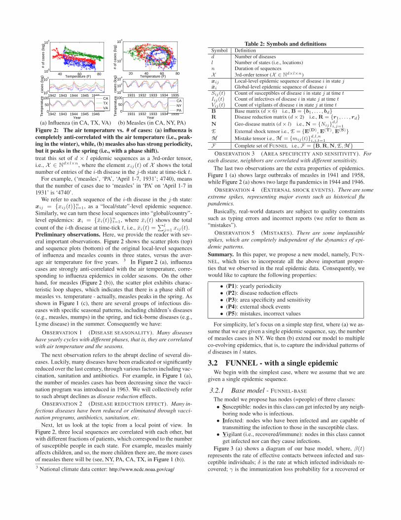
Figure 3 (a) shows a diagram of our base model, where, β(t)represents the rate of effective contacts between infected and sus-ceptible individuals; δ is the rate at which infected individuals re-covered; γ is the immunization loss probability for a recovered or

!!

"!

#!γ

δ

β(t)!!

"!

#!γ

δ

β(t)

θ(t)

ε(t)

(a) FUNNEL-BASE (b) FUNNEL-RE

Figure 3: FUNNEL diagrams: there are three classes - suscep-

tible (i.e., healthy, but can get infected), infected (i.e., capable of

transmission), vigilant (i.e., healthy, and cannot get infected).

vigilant individual. 4 More importantly, to handle the first prop-erty of epidemics: (P1), we assume that the infection rate β(t) is aperiodic function of time t. We refer to it as FUNNEL-BASE.

MODEL 1 (FUNNEL-BASE). Let S(t), I(t), V (t) be the num-

ber of susceptible, infected, vigilant people at time-tick t. Our base

model is governed by the following equations:

S(t+ 1) = S(t)− β(t)S(t)I(t) + γV (t)

I(t+ 1) = I(t) + β(t)S(t)I(t)− δI(t)

V (t+ 1) = V (t) + δI(t)− γV (t) (1)

where β(t) = β0 ·(

1 + Pa · cos(

2πPp

(t + Ps))

)

, Pp = 52, 5

and, we have the invariant N = S(t) + I(t) + V (t), with initial

conditions S(1) = N − 1, I(1) = 1, V (1) = 0.

Consequently, FUNNEL-BASE consists of a set of the following pa-rameters: b = {N, β0, δ, γ, Pa, Ps}, specifically,

• N : Potential population of the disease. N is composed ofsusceptible, infected and vigilant individuals.

• β0: Rate of effective contacts between infected and suscepti-ble individuals averaged over the year.

• δ: Healing rate of the disease.• γ: Forgetting rate of the diseases.• Pa: Amplitude of the fluctuation, specifically, it gives the

relative value of the peak/off-season.• Ps: Phase shift of the seasonal cycle.

3.2.2 With disease reduction - FUNNEL-R

With respect to the second property: (P2), we also introduce anessential concept, namely, the “disease reduction” effect.

MODEL 2 (FUNNEL-R). We add a disease reduction rate: θ(t),to capture the effect of the disease reduction program, that is,

S(t+ 1) = S(t)− β(t)S(t)I(t) + γV (t)− θ(t)S(t)

I(t+ 1) = I(t) + β(t)S(t)I(t)− δI(t)

V (t+ 1) = V (t) + δI(t)− γV (t) + θ(t)S(t) (2)

where, the disease reduction program started at time tθ and θ(t) is

defined as: θ(t) =

{

0 (t < tθ)θ0 (t ≥ tθ)

The model is identical to FUNNEL-BASE, with the addition of thedisease reduction factor, θ(t), which corresponds to the direct im-munization probability when susceptible (see Figure 3 (b)). Notethat this effect is due to vaccination, antibiotics and any other anti-disease factors. Hereafter, we simply say the “disease reductioneffect”, unless otherwise specified.

In addition to the base parameters b, FUNNEL-R requires a setof two parameters, r = {tθ, θ0}, where,

• tθ: Starting time of the disease reduction effect.• θ0: Diffusion rate of the disease reduction effect.

4 This factor also incorporates the birth and mortality rate.5We have 52 time-ticks (weeks) in one year.

3.2.3 With external shocks - FUNNEL-RE

Next, with respect to the property: (P4), we assume that thereare external shock events, such as flu pandemics. So how do wego about capturing such unexpected patterns? Assume that there isa swine flu pandemic. In this situation, many more people in thesusceptible class would become infected than in previous years.

An elementary concept we need to introduce is the temporal sus-

ceptible rate: ǫ(t). Figure 3 (b) describes how this is done. Theidea is that the number of susceptibles S(t) is the count of vic-tims available for infection, and if there is an external shock eventat time-tick t, the virus attacks are much stronger than usual, and,each victim-attack pair would lead to a new victim, and will even-tually cause a major pandemic.

MODEL 3 (FUNNEL-RE). Our full model can be described

as the following equations:

S(t+ 1) = S(t)− β(t)ǫ(t)S(t)I(t) + γV (t)− θ(t)S(t)

I(t+ 1) = I(t) + β(t)ǫ(t)S(t)I(t)− δI(t)

V (t+ 1) = V (t) + δI(t)− γV (t) + θ(t)S(t) (3)

In addition, we introduce the temporal susceptible rate, ǫ(t), which

is defined as follows:

ǫ(t) = 1+

k∑

i=1

f(t; e(T )i ), f(t; e(T )) =

{

ǫ0 (tµ − tσ < t < tµ + tσ)0 (else)

where, k is the number of shocks, and if k = 0, then ǫ(t) = 1.

Here, each external shock consists of e(T ) = {tµ, tσ, ǫ0}, i.e.,• tµ: Central time point of the external shock event.• tσ: Duration of the event.• ǫ0: Strength of the external shock effect.

3.3 FUNNEL - with multi-evolving epidemicsSo far we have seen how FUNNEL captures the dynamics of a

single epidemic sequence. The next question is, “how can we applyFUNNEL to multiple co-evolving epidemics in X , and capture theindividual behavior of d diseases in l states?”

We want to estimate the parameter set of FUNNEL, for each in-dividual epidemic sequence in X . The straightforward solutionwould be that we consider a set of (d × l) sequences of length

n generated from X : {xij}d,li,j=1, (i.e, “local-level” epidemic se-

quences), and estimate parameter set: {b, r, e(T )} for each se-quence. However, some of the (disease, state) pairs have verysparse sequences (e.g., Lyme disease in Alaska), which derails thefitting result. Also, we are interested in capturing global/country-level patterns, as well as local/state-level trends. So how can wedeal with this issue? We thus propose “sharing” the global-levelparameters for all l states, to achieve much better modeling.FUNNEL - full model parameter set. Our goal is to extract themain trends and external patterns of co-evolving epidemics X ∈N

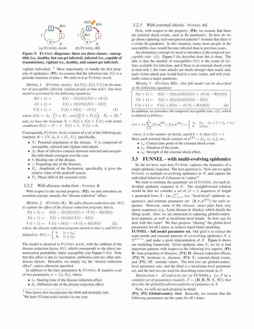
d×l×n, and make a good representation of X . Figure 4 showsour modeling framework. Given epidemic data X , we try to findimportant patterns with respect to the following five aspects, (P1)B: base properties of diseases, (P2) R: disease reduction effects,(P3) N: locations vs. diseases, (P4) E : external shock events,and (P5) M : mistake values. The first two are global/country-level parameter sets, and the third is a local/state-level parameterset, and the last two are used for describing extra trends in X .

DEFINITION 1 (COMPLETE SET OF FUNNEL). Let F be a

complete set of parameters (namely, F = {B,R,N,E ,M }) that

describe the global/local/extra patterns of epidemics in X .

Next, we will see each property in detail.(P1), (P2) Global/country view. Basically, we assume that thefollowing parameters are the same for all l states.

states!

diseases!

l

d

time!n

=

,Bd

,

N,β0,δ,γ,P

a,P

s

R

,

θ0, tθ

d

6 2

X M

l

d

n

,

N

d

l

(P1, P2): global/country view! (P3): local/state view! (P4, P5): extra view - E: shocks & M: mistakes!

E

l

d

n

(a) FUNNEL structure (i.e., F = {B,R,N,E ,M })

+ +

ek

(D)

ek

(T )ek

(S )

... + =

l

e(D)

k

k

k

E(S )

E(D)

E(T )

tµ, tσ ,ε0

13

=n

e1

(D)

e1

(T )e1

(S )

d

l

e2

(D)

e2

(T )e2

(S )

E

l

d

n

(e1)! (e2)!

(ek)!

(e1)! (e2)! (ek)!

(b) External shock tensor (i.e., E = {E(D),E(T),E(S)})

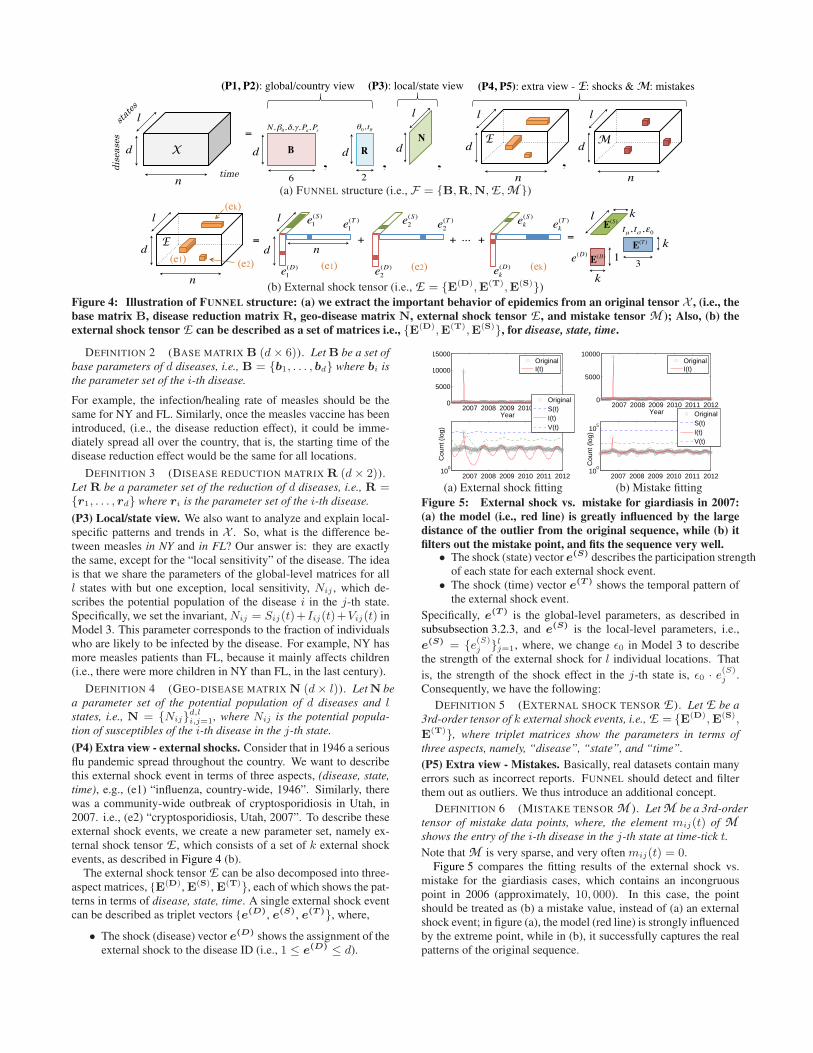
Figure 4: Illustration of FUNNEL structure: (a) we extract the important behavior of epidemics from an original tensor X , (i.e., the

base matrix B, disease reduction matrix R, geo-disease matrix N, external shock tensor E , and mistake tensor M ); Also, (b) the

external shock tensor E can be described as a set of matrices i.e., {E(D),E(T),E(S)}, for disease, state, time.

DEFINITION 2 (BASE MATRIX B (d× 6)). Let B be a set of

base parameters of d diseases, i.e., B = {b1, . . . , bd} where bi is

the parameter set of the i-th disease.

For example, the infection/healing rate of measles should be thesame for NY and FL. Similarly, once the measles vaccine has beenintroduced, (i.e., the disease reduction effect), it could be imme-diately spread all over the country, that is, the starting time of thedisease reduction effect would be the same for all locations.

DEFINITION 3 (DISEASE REDUCTION MATRIX R (d× 2)).Let R be a parameter set of the reduction of d diseases, i.e., R ={r1, . . . , rd} where ri is the parameter set of the i-th disease.

(P3) Local/state view. We also want to analyze and explain local-specific patterns and trends in X . So, what is the difference be-tween measles in NY and in FL? Our answer is: they are exactlythe same, except for the “local sensitivity” of the disease. The ideais that we share the parameters of the global-level matrices for alll states with but one exception, local sensitivity, Nij , which de-scribes the potential population of the disease i in the j-th state.Specifically, we set the invariant, Nij = Sij(t)+Iij(t)+Vij(t) inModel 3. This parameter corresponds to the fraction of individualswho are likely to be infected by the disease. For example, NY hasmore measles patients than FL, because it mainly affects children(i.e., there were more children in NY than FL, in the last century).

DEFINITION 4 (GEO-DISEASE MATRIX N (d× l)). Let N be

a parameter set of the potential population of d diseases and lstates, i.e., N = {Nij}

d,li,j=1, where Nij is the potential popula-

tion of susceptibles of the i-th disease in the j-th state.

(P4) Extra view - external shocks. Consider that in 1946 a seriousflu pandemic spread throughout the country. We want to describethis external shock event in terms of three aspects, (disease, state,

time), e.g., (e1) “influenza, country-wide, 1946”. Similarly, therewas a community-wide outbreak of cryptosporidiosis in Utah, in2007. i.e., (e2) “cryptosporidiosis, Utah, 2007”. To describe theseexternal shock events, we create a new parameter set, namely ex-ternal shock tensor E , which consists of a set of k external shockevents, as described in Figure 4 (b).

The external shock tensor E can be also decomposed into three-aspect matrices, {E(D), E(S), E(T)}, each of which shows the pat-terns in terms of disease, state, time. A single external shock eventcan be described as triplet vectors {e(D), e(S), e(T )}, where,

• The shock (disease) vector e(D) shows the assignment of theexternal shock to the disease ID (i.e., 1 ≤ e

(D) ≤ d).

2007 2008 2009 2010 2011 20120

5000

10000

15000

Year

2007 2008 2009 2010 2011 201210

0

Cou

nt (

log)

OriginalI(t)

OriginalS(t)I(t)V(t)

2007 2008 2009 2010 2011 20120

5000

10000

Year

2007 2008 2009 2010 2011 201210

0

105

Cou

nt (

log)

OriginalI(t)

OriginalS(t)I(t)V(t)

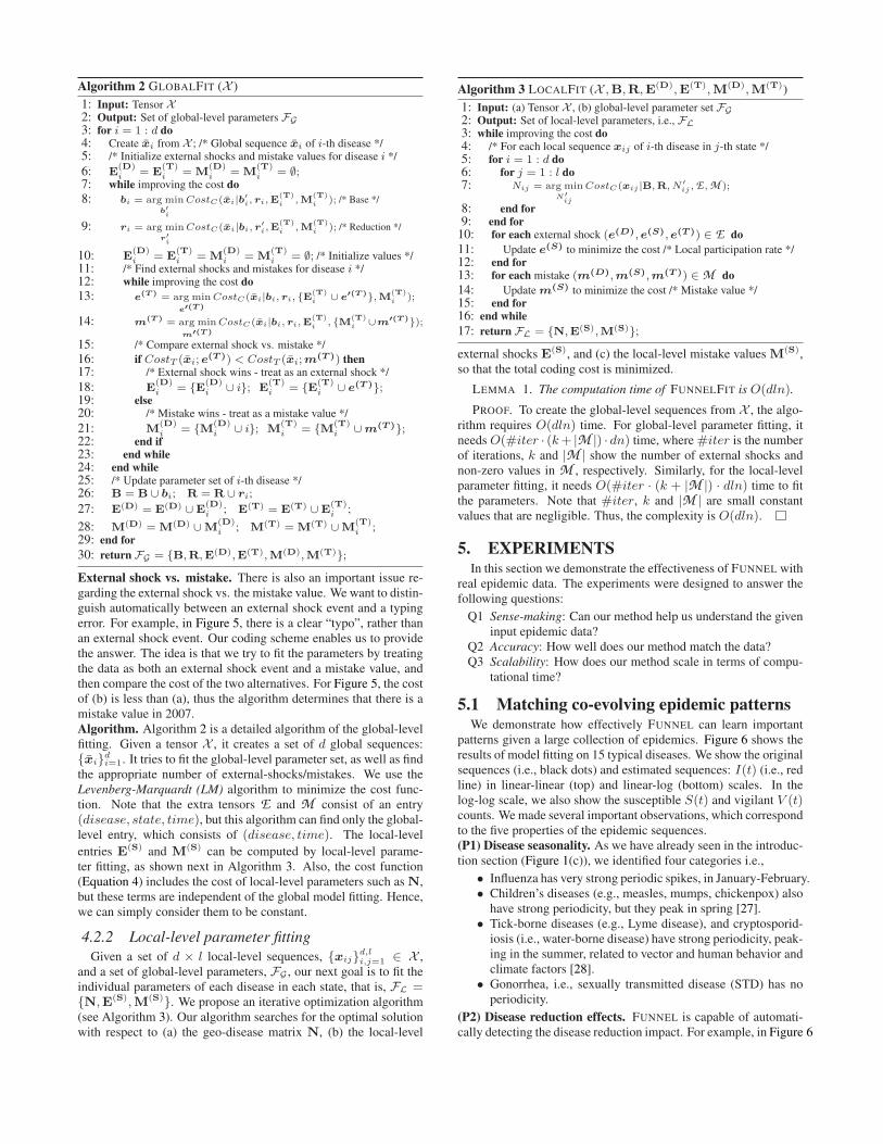
(a) External shock fitting (b) Mistake fitting

Figure 5: External shock vs. mistake for giardiasis in 2007:

(a) the model (i.e., red line) is greatly influenced by the large

distance of the outlier from the original sequence, while (b) it

filters out the mistake point, and fits the sequence very well.• The shock (state) vector e(S) describes the participation strength

of each state for each external shock event.• The shock (time) vector e(T ) shows the temporal pattern of

the external shock event.

Specifically, e(T ) is the global-level parameters, as described insubsubsection 3.2.3, and e

(S) is the local-level parameters, i.e.,

e(S) = {e

(S)j }lj=1, where, we change ǫ0 in Model 3 to describe

the strength of the external shock for l individual locations. That

is, the strength of the shock effect in the j-th state is, ǫ0 · e(S)j .

Consequently, we have the following:

DEFINITION 5 (EXTERNAL SHOCK TENSOR E ). Let E be a

3rd-order tensor of k external shock events, i.e., E = {E(D),E(S),

E(T)}, where triplet matrices show the parameters in terms of

three aspects, namely, “disease”, “state”, and “time”.

(P5) Extra view - Mistakes. Basically, real datasets contain manyerrors such as incorrect reports. FUNNEL should detect and filterthem out as outliers. We thus introduce an additional concept.

DEFINITION 6 (MISTAKE TENSOR M ). Let M be a 3rd-order

tensor of mistake data points, where, the element mij(t) of M

shows the entry of the i-th disease in the j-th state at time-tick t.

Note that M is very sparse, and very often mij(t) = 0.Figure 5 compares the fitting results of the external shock vs.

mistake for the giardiasis cases, which contains an incongruouspoint in 2006 (approximately, 10, 000). In this case, the pointshould be treated as (b) a mistake value, instead of (a) an externalshock event; in figure (a), the model (red line) is strongly influencedby the extreme point, while in (b), it successfully captures the realpatterns of the original sequence.

4. OPTIMIZATION ALGORITHMIn this section, we describe our fitting algorithm, FUNNELFIT.

Our goal is to extract the important patterns of epidemics from X .More specifically, the problem that we want to solve is as follows:

PROBLEM 1. Given a tensor X of (disease, state, time) triplets,

Find a compact description that best summarizes X , that is, F ={B,R,N,E ,M }.

We want to find a good representation F to solve the problem. Theessential questions are: (a) How can we estimate the parameter setthat best captures the dynamics and patterns in X ? (b) How shouldwe decide the number of external shocks k? (c) How can we ignoremistake (i.e., outlier) values in X ?

4.1 Model quality and data compressionWe provide a new intuitive coding scheme, which is based on the

minimum description length (MDL) principle. In short, it followsthe assumption that the more we can compress the data, the morewe can learn about its underlying patterns.Model description cost. The description complexity of model pa-rameter set consists of the following terms,

• The number of diseases d, states l, and time-ticks n requirelog∗(d) + log∗(l) + log∗(n) bits. 6

• The model parameter set of the base (B), reduction (R), geo-disease (N) matrices require d× 6, d× 2, d× l parameters,respectively, i.e., CostM (B)+CostM (R)+CostM (N) =cF · d(6 + 2 + l), where cF is the floating point cost7.

Similarly, the model description cost of the external shock tensorE = {E(D), E(S), E(T)}) consists of the following:

• The number of external shocks k requires log∗(k) bits.

• The shock-disease matrix E(D) requires k log(d).

• The shock-time parameter set e(T ) = {tµ, tσ, ǫ0} in E(T)

requires log(n), log(n), cF , respectively.

• The shock-state matrix E(S) requires cF · kl.

Consequently, the model cost of the external shock tensor E isCostM (E) = log∗(k) + k

(

log(d) + 2 log(n) + cF · (1 + l))

.

The model cost of mistake tensor M consists of

• The number of non-zero elements in M requires log∗(|M |)• The location of each non-zero element and its value, mij(t)

require log(d),log(l),log(n), log∗(mij(t)), respectively.

Thus, CostM (M ) = log∗(|M |)+∑|M |

mij(t)>0(log(d)+ log(l)+

log(n) + log∗(mij(t))), where, |M | is the number of non-zeroelements in M .Data coding cost. Once we have decided the full parameter setF , we can encode the data X using Huffman coding [3], i.e., anumber of bits is assigned to each value in X , which is the log-arithm of the inverse of the probability of the values (here, weuse a Gaussian distribution). The encoding cost of X given Fis: CostC(X|F) =

∑d,l,n

i,j,t=1 log2 p−1Gauss(µ,σ)(xij(t)−mij(t)−

Iij(t)), where, xij(t), mij(t) are the elements in X and the mis-take tensor M , respectively, and Iij(t) is the estimated count ofinfections (i.e., Model 3). Also, µ and σ are the mean and varianceof the distance between the original and estimated values. 8

Putting it all together. Consequently, the total code length for Xwith respect to a given parameter set F can be described as follows:

6Here, log∗ is the universal code length for integers.7We used 4× 8 bits in our setting.8 Here, µ, σ need 2cF bits, but we can eliminate them because theyare constant values and independent of our modeling.

CostT (X ;F) = log∗(d) + log∗(l) + log∗(n)

+CostM (B) + CostM (R) + CostM (N)

+CostM (E) + CostM (M ) + CostC(X|F) (4)

Thus our next goal is to minimize the above function.

4.2 Multi-layer optimizationUntil now, we have seen how we can measure the goodness of

the representation of X , if we are given a candidate parameter setF . The next question is, how to find an optimal solution of the fullparameter set: F = {B,R,N,E ,M }.

As described in subsection 3.3, our FUNNEL model consists ofmultiple parameter sets, each of which explains either the local orglobal pattern of epidemics in X . For example, the base and re-duction matrices B, R explain the global-level behavior of eachdisease, while the geo-disease matrix N describes the local-leveltrends. Also, the extra tensors E , M consist of both the globaland local-level parameters. More specifically, the external shocksconsists of E = {E(D), E(S), E(T)}), where, the first two arethe global-level, and the last one is the local-level. Similarly, themistake tensor can also be describes by the triplet matrix M ={M(D), M(S), M(T)}), each of which describes the location ofthe mistake values in terms of disease, state, time. So, how can weefficiently estimate these model parameters?

We propose a multi-layer optimization algorithm, to search forthe optimal solution in terms of both the global and local-level pa-rameters. The idea is that we split parameter set F into two subsets,i.e., FG and FL, each of which corresponds to a global/local-levelparameter set, and try to fit the parameter sets separately. Our algo-rithm consists of the following two phases:

• GLOBALFIT: find good global-level parameters for {x̄i}di=1,

i.e., FG = {B,R, E(D),E(T),M(D),M(T)}

• LOCALFIT: find good local-level parameters: for {xij}d,li,j=1,

i.e., FL = {N,E(S),M(S)}

Here, the global epidemic sequence of the i-th disease: x̄i canbe described as the sum of the l local sequences, i.e., x̄i(t) =∑l

j=1 xij(t). Algorithm 1 shows an overview of FUNNELFIT.Given a tensor X , it finds the full set of FUNNEL parameters.

Algorithm 1 FUNNELFIT (X )

1: Input: Tensor X (d× l × n)2: Output: Complete set of parameters, i.e., F = {B,R,N,E ,M }3: /* Parameter fitting for global-level sequences */4: {FG} =GLOBALFIT (X );5: /* Parameter fitting for local-level sequences */6: {FL} =LOCALFIT (X ,FG);

7: return F = {FG ,FL};

4.2.1 Global-level parameter fitting

Given a tensor X , our sub-goal is to find the optimal global-levelparameter set: FG , to minimize the cost function (i.e., Equation 4).We want to fit the basic parameters of each disease (i.e., the baseand reduction matrices), and estimate the appropriate number ofexternal shocks and mistake values, simultaneously. Finding theappropriate number of external-shocks/mistakes is a particular is-sue here, because the parameter fittings are very sensitive to out-liers, as described in Figure 5 (a). To find a good basic parameterset for X , we have to filter out the external shocks and mistakesappropriately. Simultaneously, a good external-shock/mistake fil-ter requires a well estimated base model. We escape this circulardependency by applying an iterative method that employs external-shocks/mistakes detection and filtering, and basic model fitting inan alternating way until the cost function reaches a minimum value.

Algorithm 2 GLOBALFIT (X )

1: Input: Tensor X2: Output: Set of global-level parameters FG

3: for i = 1 : d do4: Create x̄i from X ; /* Global sequence x̄i of i-th disease */5: /* Initialize external shocks and mistake values for disease i */

6: E(D)i = E

(T)i = M

(D)i = M

(T)i = ∅;

7: while improving the cost do

8: bi = arg minb′i

CostC(x̄i|b′

i, ri,E(T)i

,M(T)i

); /* Base */

9: ri = arg minr′

i

CostC(x̄i|bi, r′

i,E(T)i

,M(T)i

); /* Reduction */

10: E(D)i = E

(T)i = M

(D)i = M

(T)i = ∅; /* Initialize values */

11: /* Find external shocks and mistakes for disease i */12: while improving the cost do

13: e(T ) = arg min

e′(T )

CostC(x̄i|bi, ri, {E(T)i

∪ e′(T )},M

(T)i

);

14: m(T ) = arg min

m′(T )

CostC(x̄i|bi, ri,E(T)i

, {M(T)i

∪m′(T )});

15: /* Compare external shock vs. mistake */

16: if CostT (x̄i; e(T )) < CostT (x̄i;m

(T )) then17: /* External shock wins - treat as an external shock */

18: E(D)i = {E(D)

i ∪ i}; E(T)i = {E(T)

i ∪ e(T )};

19: else20: /* Mistake wins - treat as a mistake value */

21: M(D)i = {M(D)

i ∪ i}; M(T)i = {M(T)

i ∪m(T )};

22: end if23: end while24: end while25: /* Update parameter set of i-th disease */26: B = B ∪ bi; R = R ∪ ri;

27: E(D) = E

(D) ∪E(D)i ; E

(T) = E(T) ∪E

(T)i ;

28: M(D) = M

(D) ∪M(D)i ; M

(T) = M(T) ∪M

(T)i ;

29: end for

30: return FG = {B,R,E(D),E(T),M(D),M(T)};

External shock vs. mistake. There is also an important issue re-garding the external shock vs. the mistake value. We want to distin-guish automatically between an external shock event and a typingerror. For example, in Figure 5, there is a clear “typo”, rather thanan external shock event. Our coding scheme enables us to providethe answer. The idea is that we try to fit the parameters by treatingthe data as both an external shock event and a mistake value, andthen compare the cost of the two alternatives. For Figure 5, the costof (b) is less than (a), thus the algorithm determines that there is amistake value in 2007.Algorithm. Algorithm 2 is a detailed algorithm of the global-levelfitting. Given a tensor X , it creates a set of d global sequences:{x̄i}

di=1. It tries to fit the global-level parameter set, as well as find

the appropriate number of external-shocks/mistakes. We use theLevenberg-Marquardt (LM) algorithm to minimize the cost func-tion. Note that the extra tensors E and M consist of an entry(disease, state, time), but this algorithm can find only the global-level entry, which consists of (disease, time). The local-level

entries E(S) and M

(S) can be computed by local-level parame-ter fitting, as shown next in Algorithm 3. Also, the cost function(Equation 4) includes the cost of local-level parameters such as N,but these terms are independent of the global model fitting. Hence,we can simply consider them to be constant.

4.2.2 Local-level parameter fitting

Given a set of d × l local-level sequences, {xij}d,li,j=1 ∈ X ,

and a set of global-level parameters, FG , our next goal is to fit theindividual parameters of each disease in each state, that is, FL ={N,E(S),M(S)}. We propose an iterative optimization algorithm(see Algorithm 3). Our algorithm searches for the optimal solutionwith respect to (a) the geo-disease matrix N, (b) the local-level

Algorithm 3 LOCALFIT (X ,B,R,E(D),E(T),M(D),M(T))

1: Input: (a) Tensor X , (b) global-level parameter set FG

2: Output: Set of local-level parameters, i.e., FL

3: while improving the cost do4: /* For each local sequence xij of i-th disease in j-th state */5: for i = 1 : d do6: for j = 1 : l do7: Nij = arg min

N′

ij

CostC(xij |B,R, N ′

ij , E , M );

8: end for9: end for

10: for each external shock (e(D), e(S), e(T )) ∈ E do

11: Update e(S) to minimize the cost /* Local participation rate */

12: end for13: for each mistake (m(D),m(S),m(T )) ∈ M do

14: Update m(S) to minimize the cost /* Mistake value */

15: end for16: end while

17: return FL = {N,E(S),M(S)};

external shocks E(S), and (c) the local-level mistake values M(S),so that the total coding cost is minimized.

LEMMA 1. The computation time of FUNNELFIT is O(dln).

PROOF. To create the global-level sequences from X , the algo-rithm requires O(dln) time. For global-level parameter fitting, itneeds O(#iter · (k+ |M |) · dn) time, where #iter is the numberof iterations, k and |M | show the number of external shocks andnon-zero values in M , respectively. Similarly, for the local-levelparameter fitting, it needs O(#iter · (k + |M |) · dln) time to fitthe parameters. Note that #iter, k and |M | are small constantvalues that are negligible. Thus, the complexity is O(dln).

5. EXPERIMENTSIn this section we demonstrate the effectiveness of FUNNEL with

real epidemic data. The experiments were designed to answer thefollowing questions:

Q1 Sense-making: Can our method help us understand the giveninput epidemic data?

Q2 Accuracy: How well does our method match the data?Q3 Scalability: How does our method scale in terms of compu-

tational time?

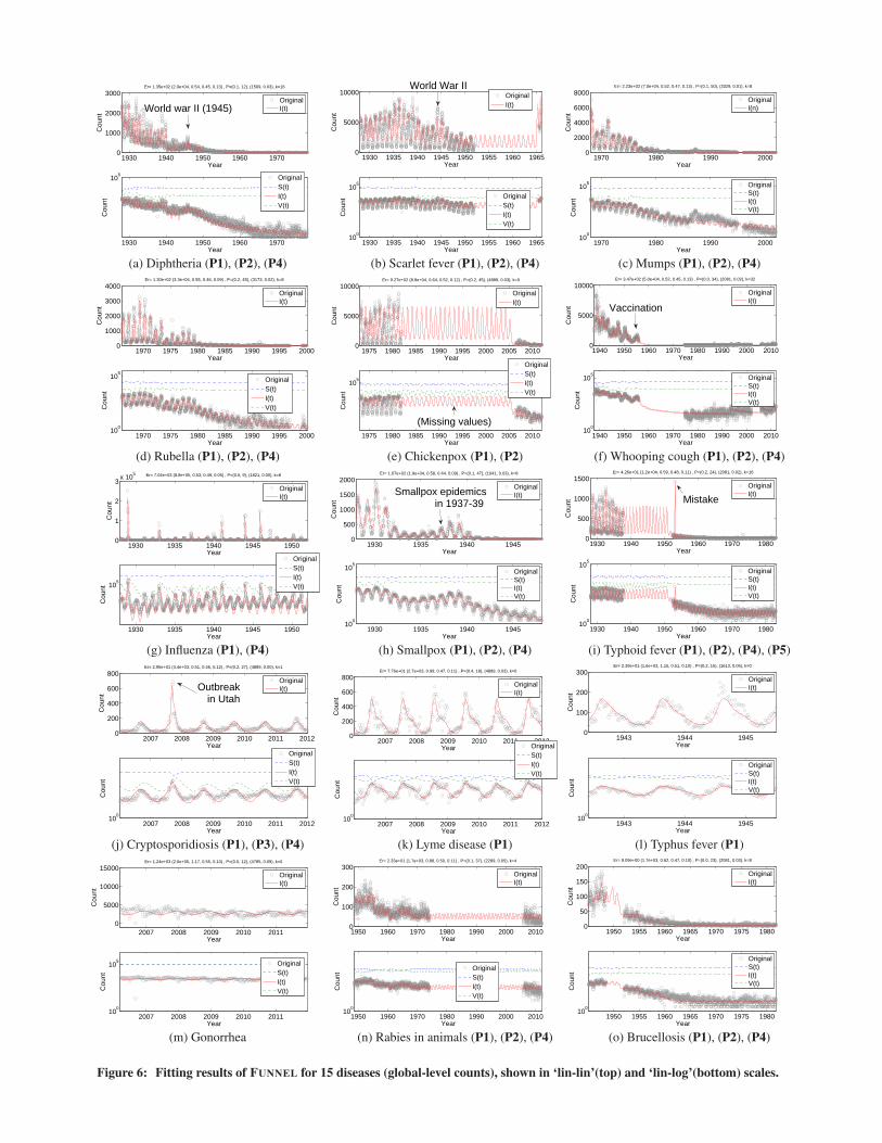
5.1 Matching co-evolving epidemic patternsWe demonstrate how effectively FUNNEL can learn important

patterns given a large collection of epidemics. Figure 6 shows theresults of model fitting on 15 typical diseases. We show the originalsequences (i.e., black dots) and estimated sequences: I(t) (i.e., redline) in linear-linear (top) and linear-log (bottom) scales. In thelog-log scale, we also show the susceptible S(t) and vigilant V (t)counts. We made several important observations, which correspondto the five properties of the epidemic sequences.(P1) Disease seasonality. As we have already seen in the introduc-tion section (Figure 1(c)), we identified four categories i.e.,

• Influenza has very strong periodic spikes, in January-February.• Children’s diseases (e.g., measles, mumps, chickenpox) also

have strong periodicity, but they peak in spring [27].• Tick-borne diseases (e.g., Lyme disease), and cryptosporid-

iosis (i.e., water-borne disease) have strong periodicity, peak-ing in the summer, related to vector and human behavior andclimate factors [28].

• Gonorrhea, i.e., sexually transmitted disease (STD) has noperiodicity.

(P2) Disease reduction effects. FUNNEL is capable of automati-cally detecting the disease reduction impact. For example, in Figure 6

1930 1940 1950 1960 19700

1000

2000

3000

Year

Cou

nt

Er= 1.35e+02 (2.0e+04, 0.54, 0.45, 0.13) , P=(0.1, 12), (1509, 0.03), k=16

1930 1940 1950 1960 1970

105

Year

Cou

nt

OriginalI(t)

OriginalS(t)I(t)V(t)

World war II (1945)

1930 1935 1940 1945 1950 1955 1960 19650

5000

10000

Year

Cou

nt

1930 1935 1940 1945 1950 1955 1960 196510

0

105

Year

Cou

nt

OriginalI(t)

OriginalS(t)I(t)V(t)

World War II

1970 1980 1990 20000

2000

4000

6000

8000

Year

Cou

nt

Er= 2.23e+02 (7.0e+04, 0.52, 0.47, 0.13) , P=(0.1, 50), (3329, 0.01), k=8

1970 1980 1990 200010

0

105

Year

Cou

nt

OriginalI(n)

OriginalS(t)I(t)V(t)

(a) Diphtheria (P1), (P2), (P4) (b) Scarlet fever (P1), (P2), (P4) (c) Mumps (P1), (P2), (P4)

1970 1975 1980 1985 1990 1995 20000

1000

2000

3000

4000

Year

Cou

nt

Er= 1.30e+02 (3.3e+04, 0.55, 0.46, 0.09) , P=(0.2, 45), (3173, 0.02), k=8

1970 1975 1980 1985 1990 1995 200010

0

105

Year

Cou

nt

OriginalI(t)

OriginalS(t)I(t)V(t)

1975 1980 1985 1990 1995 2000 2005 20100

5000

10000

Year

Cou

nt

Er= 9.27e+02 (8.8e+04, 0.64, 0.52, 0.12) , P=(0.2, 45), (4889, 0.03), k=0

1975 1980 1985 1990 1995 2000 2005 2010

105

Year

Cou

nt

OriginalI(t)

OriginalS(t)I(t)V(t)

(Missing values)

1940 1950 1960 1970 1980 1990 2000 20100

5000

10000

Year

Cou

nt

Er= 3.47e+02 (5.0e+04, 0.52, 0.45, 0.13) , P=(0.0, 34), (2081, 0.02), k=32

1940 1950 1960 1970 1980 1990 2000 201010

0

105

Year

Cou

nt

OriginalI(t)

OriginalS(t)I(t)V(t)

Vaccination

(d) Rubella (P1), (P2), (P4) (e) Chickenpox (P1), (P2) (f) Whooping cough (P1), (P2), (P4)

1930 1935 1940 1945 19500

1

2

3x 10

5

Year

Cou

nt

Er= 7.04e+03 (8.8e+05, 0.53, 0.49, 0.05) , P=(0.5, 9), (1821, 0.00), k=8

1930 1935 1940 1945 1950

105

Year

Cou

nt

OriginalI(t)

OriginalS(t)I(t)V(t)

1930 1935 1940 19450

500

1000

1500

2000

Year

Cou

nt

Er= 1.07e+02 (1.9e+04, 0.58, 0.44, 0.09) , P=(0.1, 47), (1041, 0.03), k=8

1930 1935 1940 194510

0

105

Year

Cou

nt

OriginalI(t)

OriginalS(t)I(t)V(t)

Smallpox epidemicsin 1937-39

1930 1940 1950 1960 1970 19800

500

1000

1500

Year

Cou

nt

Er= 4.26e+01 (1.2e+04, 0.59, 0.48, 0.11) , P=(0.2, 24), (2081, 0.02), k=16

1930 1940 1950 1960 1970 198010

0

105

Year

Cou

nt

OriginalI(t)

OriginalS(t)I(t)V(t)

Mistake

(g) Influenza (P1), (P4) (h) Smallpox (P1), (P2), (P4) (i) Typhoid fever (P1), (P2), (P4), (P5)

2007 2008 2009 2010 2011 20120

200

400

600

800

Year

Cou

nt

Er= 2.95e+01 (3.4e+03, 0.51, 0.46, 0.12) , P=(0.2, 27), (4889, 0.00), k=1

2007 2008 2009 2010 2011 201210

0

Year

Cou

nt

OriginalI(t)

OriginalS(t)I(t)V(t)

Outbreak in Utah

2007 2008 2009 2010 2011 20120

200

400

600

800

Year

Cou

nt

Er= 7.76e+01 (2.7e+03, 0.99, 0.47, 0.11) , P=(0.4, 18), (4889, 0.03), k=0

2007 2008 2009 2010 2011 201210

0

Year

Cou

nt

OriginalI(t)

OriginalS(t)I(t)V(t)

1943 1944 19450

100

200

300

Year

Cou

nt

Er= 2.39e+01 (1.6e+03, 1.15, 0.51, 0.10) , P=(0.2, 15), (1613, 0.05), k=0

1943 1944 194510

0

Year

Cou

nt

OriginalI(t)

OriginalS(t)I(t)V(t)

(j) Cryptosporidiosis (P1), (P3), (P4) (k) Lyme disease (P1) (l) Typhus fever (P1)

2007 2008 2009 2010 20110

5000

10000

15000

Year

Cou

nt

Er= 1.24e+03 (2.0e+05, 1.17, 0.55, 0.10) , P=(0.0, 12), (4785, 0.09), k=0

2007 2008 2009 2010 201110

0

105

Year

Cou

nt

OriginalI(t)

OriginalS(t)I(t)V(t)

1950 1960 1970 1980 1990 2000 20100

100

200

300

Year

Cou

nt

Er= 2.33e+01 (1.7e+03, 0.88, 0.50, 0.11) , P=(0.1, 37), (2289, 0.05), k=4

1950 1960 1970 1980 1990 2000 201010

0

Year

Cou

nt

OriginalI(t)

OriginalS(t)I(t)V(t)

1950 1955 1960 1965 1970 1975 19800

50

100

150

200

Year

Cou

nt

Er= 9.09e+00 (1.7e+03, 0.62, 0.47, 0.10) , P=(0.0, 23), (2081, 0.03), k=8

1950 1955 1960 1965 1970 1975 198010

0

Year

Cou

nt

OriginalI(t)

OriginalS(t)I(t)V(t)

(m) Gonorrhea (n) Rabies in animals (P1), (P2), (P4) (o) Brucellosis (P1), (P2), (P4)

Figure 6: Fitting results of FUNNEL for 15 diseases (global-level counts), shown in ‘lin-lin’(top) and ‘lin-log’(bottom) scales.

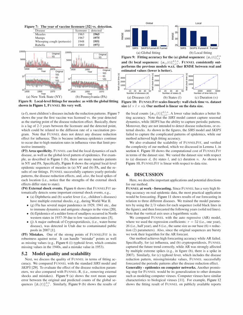
Figure 7: The year of vaccine licensure [32] vs. detection.Disease licensure detected

Measles 1963 1965Mumps 1967 1975Whooping cough (pertussis) 1948 1951Rubella 1969 1972

1930 1950 19700

5000

10000

Year

1930 1950 197010

0

105

Year

OriginalI(t)

OriginalS(t)I(t)V(t)

1930 1950 19700

5000

10000

Year

1930 1950 197010

0

105

Year

OriginalI(t)

OriginalS(t)I(t)V(t)

(a) New York State (NY) (b) Pennsylvania (PA)

Figure 8: Local-level fittings for measles: as with the global fitting

shown in Figure 1, FUNNEL fits very well.

SIRS SKIPSFunnel-R Funnel500

1000

1500

Global

RM

SE

SIRS SKIPS Funnel-R Funnel25

30

35

40Local

RM

SE

(a) Global fitting (b) Local fitting

Figure 9: Fitting accuracy for the (a) global sequences: {x̄i(t)}d,ni,t

and (b) local sequences: {xij(t)}d,l,ni,j,t . FUNNEL consistently out-

performs the previous models w.r.t. ther RMSE between real and

estimated values (lower is better).

10 20 30 40 500

1000

2000

3000

Number of diseases (d)

Wal

l clo

ck ti

me

(s)

10 20 30 40 50

2000

2500

3000

Number of states (l)

Wal

l clo

ck ti

me

(s)

2000 4000 60000

1000

2000

3000

Number of time-ticks (n)

Wal

l clo

ck ti

me

(s)

(a) Diseases (d) (b) States (l) (c) Duration (n)

Figure 10: FUNNELFIT scales linearly: wall clock time vs. dataset

size (d× l × n). Our method is linear on the data size.

(a-f), most children’s diseases include the reduction patterns. Figure 7shows the year the first vaccine was licensed vs. the year detectedas the starting point of the disease reduction effect. Basically, thereis a lag of 2-3 years between the licensure and the detected point,which could be related to the diffusion rate of a vaccination pro-gram. Note that FUNNEL does not detect any disease reductioneffect for influenza; This is because influenza epidemics continueto occur due to high mutation rates in influenza virus that limit pro-tective immunity.(P3) Area specificity. FUNNEL can find the local dynamics of eachdisease, as well as the global-level pattern of epidemics. For exam-ple, as described in Figure 1 (b), there are many measles patientsin NY and PA. Specifically, Figure 8 shows the original local-levelepidemic sequences of measles in (a) NY and (b) PA, and the re-sults of our fittings. FUNNEL successfully captures yearly-periodicpatterns, the disease reduction effects, and, also, the local spikes ofeach location (i.e., notice that the strengths of the external shockeffects differ state to state).(P4) External shock events. Figure 6 shows that FUNNELFIT au-tomatically detects some important external shock events, e.g.,

• (a) Diphtheria and (b) scarlet fever (i.e., children’s diseases)have multiple external shocks, e.g., during World War II.

• (g) Flu has several major pandemics in 1929, 1941 etc., dueto immune dynamics and antigenic changes in the virus [20].

• (h) Epidemics of a milder form of smallpox occurred in North-western states in 1937-39 due to low vaccination rates [5].

• (j) A major outbreak of Cryptosporidiosis, (i.e., water-bornedisease), was detected in Utah due to contaminated publicpools in 2007 [1].

(P5) Mistakes. One of the strong points of FUNNELFIT is itsrobustness against noise. It can handle “mistake” points as wellas missing values (e.g., Figure 6 (i) typhoid fever, which containsmissing values in the 1940s, and a mistake value in 1953).

5.2 Model quality and scalabilityNext, we discuss the quality of FUNNEL in terms of fitting ac-

curacy. We compared FUNNEL with the standard SIRS model andSKIPS [29]. To evaluate the effect of the disease reduction param-eters, we also compared with FUNNEL-R, (i.e., removing externalshocks and mistakes). Figure 9 (a) shows the root mean squareerror between the original and predicted counts of the global se-quences {x̄i(t)}

d,ni,t . Similarly, Figure 9 (b) shows the results of

the local counts {xij(t)}d,l,ni,j,t , A lower value indicates a better fit-

ting accuracy. Note that the SIRS model cannot capture seasonaldynamics, while SKIPS has the ability to capture periodic patterns.Moreover, they are not intended to detect disease reductions, or ex-ternal shocks. As shown in the figures, the SIRS model and SKIPS

failed to capture the complicated patterns of epidemics, while ourmethod achieved high fitting accuracy.

We also evaluated the scalability of FUNNELFIT, and verifiedthe complexity of our method, which we discussed in Lemma 1, insection 4. Figure 10 shows the computational cost of FUNNELFIT

in terms of the dataset size. We varied the dataset size with respectto (a) diseases d, (b) states l, and (c) duration n. As shown inFigure 10, FUNNELFIT is linear with respect to data size.

6. DISCUSSIONHere, we describe important applications and potential directions

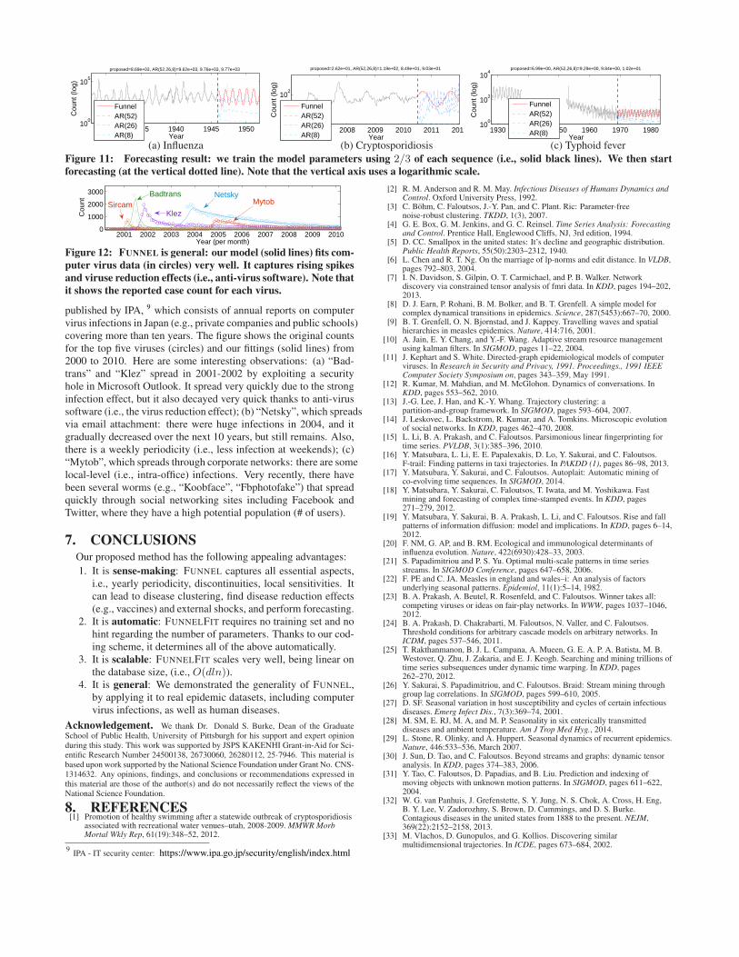
for our method.FUNNEL at work - forecasting. Since FUNNEL has a very high fit-ting accuracy on real epidemic data, the most practical applicationwould be forecasting. Figure 11 shows results of our forecasting inrelation to three different diseases. We trained the model parame-ters by using the 2/3 values for each sequence (solid black lines inthe figure), and then forecasted the following years (solid red lines).Note that the vertical axis uses a logarithmic scale.

We compared FUNNEL with the auto regressive (AR) model,where we used the regression coefficients: r = 52 (i.e., one year),26 (i.e., half year), and 8 (i.e., the same size as our base (6) + reduc-tion (2) parameters). Also, since the original sequences are burstywe took their logarithm for the AR forecast.

Our method achieves high forecasting accuracy while AR failed.Specifically, for (a) influenza, and (b) cryptosporidiosis, FUNNEL

captured the future trend correctly, while AR was strongly affectedby multiple extreme spikes (e.g., in figure (b), there is a spike in2007). Similarly, for (c) typhoid fever, which includes the diseasereduction pattern, missing/mistake values, FUNNEL successfullyforecasted the periodic patterns after the disease reduction effect.Generality - epidemics on computer networks. Another promis-ing step for FUNNEL would be its generalization to other domainssuch as modeling computer viruses. Computer viruses have similarcharacteristics to biological viruses [11]. For example, Figure 12shows the fitting result of FUNNEL on publicly available reports

1930 1935 1940 1945 195010

0

105

Year

Cou

nt (

log)

proposed=8.69e+03, AR(52,26,8)=9.62e+03, 9.76e+03, 9.77e+03

FunnelAR(52)AR(26)AR(8)

2007 2008 2009 2010 2011 201210

0

102

Year

Cou

nt (

log)

proposed=2.62e+01, AR(52,26,8)=1.19e+02, 8.49e+01, 9.03e+01

FunnelAR(52)AR(26)AR(8)

1930 1940 1950 1960 1970 198010

0

102

104

Year

Cou

nt (

log)

proposed=6.99e+00, AR(52,26,8)=9.29e+00, 9.84e+00, 1.02e+01

FunnelAR(52)AR(26)AR(8)

(a) Influenza (b) Cryptosporidiosis (c) Typhoid fever

Figure 11: Forecasting result: we train the model parameters using 2/3 of each sequence (i.e., solid black lines). We then start

forecasting (at the vertical dotted line). Note that the vertical axis uses a logarithmic scale.

2001 2002 2003 2004 2005 2006 2007 2008 2009 20100

1000

2000

3000

Year (per month)

Cou

nt

SircamKlez

Badtrans NetskyMytob

Figure 12: FUNNEL is general: our model (solid lines) fits com-

puter virus data (in circles) very well. It captures rising spikes

and viruse reduction effects (i.e., anti-virus software). Note that

it shows the reported case count for each virus.

published by IPA, 9 which consists of annual reports on computervirus infections in Japan (e.g., private companies and public schools)covering more than ten years. The figure shows the original countsfor the top five viruses (circles) and our fittings (solid lines) from2000 to 2010. Here are some interesting observations: (a) “Bad-trans” and “Klez” spread in 2001-2002 by exploiting a securityhole in Microsoft Outlook. It spread very quickly due to the stronginfection effect, but it also decayed very quick thanks to anti-virussoftware (i.e., the virus reduction effect); (b) “Netsky”, which spreadsvia email attachment: there were huge infections in 2004, and itgradually decreased over the next 10 years, but still remains. Also,there is a weekly periodicity (i.e., less infection at weekends); (c)“Mytob”, which spreads through corporate networks: there are somelocal-level (i.e., intra-office) infections. Very recently, there havebeen several worms (e.g., “Koobface”, “Fbphotofake”) that spreadquickly through social networking sites including Facebook andTwitter, where they have a high potential population (# of users).

7. CONCLUSIONSOur proposed method has the following appealing advantages:

1. It is sense-making: FUNNEL captures all essential aspects,i.e., yearly periodicity, discontinuities, local sensitivities. Itcan lead to disease clustering, find disease reduction effects(e.g., vaccines) and external shocks, and perform forecasting.

2. It is automatic: FUNNELFIT requires no training set and nohint regarding the number of parameters. Thanks to our cod-ing scheme, it determines all of the above automatically.

3. It is scalable: FUNNELFIT scales very well, being linear onthe database size, (i.e., O(dln)).

4. It is general: We demonstrated the generality of FUNNEL,by applying it to real epidemic datasets, including computervirus infections, as well as human diseases.

Acknowledgement. We thank Dr. Donald S. Burke, Dean of the GraduateSchool of Public Health, University of Pittsburgh for his support and expert opinionduring this study. This work was supported by JSPS KAKENHI Grant-in-Aid for Sci-entific Research Number 24500138, 26730060, 26280112, 25·7946. This material isbased upon work supported by the National Science Foundation under Grant No. CNS-1314632. Any opinions, findings, and conclusions or recommendations expressed inthis material are those of the author(s) and do not necessarily reflect the views of theNational Science Foundation.

8. REFERENCES[1] Promotion of healthy swimming after a statewide outbreak of cryptosporidiosis

associated with recreational water venues–utah, 2008-2009. MMWR MorbMortal Wkly Rep, 61(19):348–52, 2012.

9IPA - IT security center: https://www.ipa.go.jp/security/english/index.html

[2] R. M. Anderson and R. M. May. Infectious Diseases of Humans Dynamics andControl. Oxford University Press, 1992.

[3] C. Böhm, C. Faloutsos, J.-Y. Pan, and C. Plant. Ric: Parameter-freenoise-robust clustering. TKDD, 1(3), 2007.

[4] G. E. Box, G. M. Jenkins, and G. C. Reinsel. Time Series Analysis: Forecastingand Control. Prentice Hall, Englewood Cliffs, NJ, 3rd edition, 1994.

[5] D. CC. Smallpox in the united states: It’s decline and geographic distribution.Public Health Reports, 55(50):2303–2312, 1940.

[6] L. Chen and R. T. Ng. On the marriage of lp-norms and edit distance. In VLDB,pages 792–803, 2004.

[7] I. N. Davidson, S. Gilpin, O. T. Carmichael, and P. B. Walker. Networkdiscovery via constrained tensor analysis of fmri data. In KDD, pages 194–202,2013.

[8] D. J. Earn, P. Rohani, B. M. Bolker, and B. T. Grenfell. A simple model forcomplex dynamical transitions in epidemics. Science, 287(5453):667–70, 2000.

[9] B. T. Grenfell, O. N. Bjornstad, and J. Kappey. Travelling waves and spatialhierarchies in measles epidemics. Nature, 414:716, 2001.

[10] A. Jain, E. Y. Chang, and Y.-F. Wang. Adaptive stream resource managementusing kalman filters. In SIGMOD, pages 11–22, 2004.

[11] J. Kephart and S. White. Directed-graph epidemiological models of computerviruses. In Research in Security and Privacy, 1991. Proceedings., 1991 IEEEComputer Society Symposium on, pages 343–359, May 1991.

[12] R. Kumar, M. Mahdian, and M. McGlohon. Dynamics of conversations. InKDD, pages 553–562, 2010.

[13] J.-G. Lee, J. Han, and K.-Y. Whang. Trajectory clustering: apartition-and-group framework. In SIGMOD, pages 593–604, 2007.

[14] J. Leskovec, L. Backstrom, R. Kumar, and A. Tomkins. Microscopic evolutionof social networks. In KDD, pages 462–470, 2008.

[15] L. Li, B. A. Prakash, and C. Faloutsos. Parsimonious linear fingerprinting fortime series. PVLDB, 3(1):385–396, 2010.

[16] Y. Matsubara, L. Li, E. E. Papalexakis, D. Lo, Y. Sakurai, and C. Faloutsos.F-trail: Finding patterns in taxi trajectories. In PAKDD (1), pages 86–98, 2013.

[17] Y. Matsubara, Y. Sakurai, and C. Faloutsos. Autoplait: Automatic mining ofco-evolving time sequences. In SIGMOD, 2014.

[18] Y. Matsubara, Y. Sakurai, C. Faloutsos, T. Iwata, and M. Yoshikawa. Fastmining and forecasting of complex time-stamped events. In KDD, pages271–279, 2012.

[19] Y. Matsubara, Y. Sakurai, B. A. Prakash, L. Li, and C. Faloutsos. Rise and fallpatterns of information diffusion: model and implications. In KDD, pages 6–14,2012.

[20] F. NM, G. AP, and B. RM. Ecological and immunological determinants ofinfluenza evolution. Nature, 422(6930):428–33, 2003.

[21] S. Papadimitriou and P. S. Yu. Optimal multi-scale patterns in time seriesstreams. In SIGMOD Conference, pages 647–658, 2006.

[22] F. PE and C. JA. Measles in england and wales–i: An analysis of factorsunderlying seasonal patterns. Epidemiol, 11(1):5–14, 1982.

[23] B. A. Prakash, A. Beutel, R. Rosenfeld, and C. Faloutsos. Winner takes all:competing viruses or ideas on fair-play networks. In WWW, pages 1037–1046,2012.

[24] B. A. Prakash, D. Chakrabarti, M. Faloutsos, N. Valler, and C. Faloutsos.Threshold conditions for arbitrary cascade models on arbitrary networks. InICDM, pages 537–546, 2011.

[25] T. Rakthanmanon, B. J. L. Campana, A. Mueen, G. E. A. P. A. Batista, M. B.Westover, Q. Zhu, J. Zakaria, and E. J. Keogh. Searching and mining trillions oftime series subsequences under dynamic time warping. In KDD, pages262–270, 2012.

[26] Y. Sakurai, S. Papadimitriou, and C. Faloutsos. Braid: Stream mining throughgroup lag correlations. In SIGMOD, pages 599–610, 2005.

[27] D. SF. Seasonal variation in host susceptibility and cycles of certain infectiousdiseases. Emerg Infect Dis., 7(3):369–74, 2001.

[28] M. SM, E. RJ, M. A, and M. P. Seasonality in six enterically transmitteddiseases and ambient temperature. Am J Trop Med Hyg., 2014.

[29] L. Stone, R. Olinky, and A. Huppert. Seasonal dynamics of recurrent epidemics.Nature, 446:533–536, March 2007.

[30] J. Sun, D. Tao, and C. Faloutsos. Beyond streams and graphs: dynamic tensoranalysis. In KDD, pages 374–383, 2006.

[31] Y. Tao, C. Faloutsos, D. Papadias, and B. Liu. Prediction and indexing ofmoving objects with unknown motion patterns. In SIGMOD, pages 611–622,2004.

[32] W. G. van Panhuis, J. Grefenstette, S. Y. Jung, N. S. Chok, A. Cross, H. Eng,B. Y. Lee, V. Zadorozhny, S. Brown, D. Cummings, and D. S. Burke.Contagious diseases in the united states from 1888 to the present. NEJM,369(22):2152–2158, 2013.

[33] M. Vlachos, D. Gunopulos, and G. Kollios. Discovering similarmultidimensional trajectories. In ICDE, pages 673–684, 2002.