further investigation of integration chapter 10 further ...fjones/chap10.pdf · further...
TRANSCRIPT

Further investigation of integration 1
Chapter 10 Further investigation of integration
We have two exceedingly important things to discuss in this chapter: integration overgeneral subsets of Rn, and change of variables. We first discuss a characterization of contentedsets.
A. Topological backgroundWe have often hinted at many of the following concepts. It is now time to make certain
we understand them completely, and have useful names and notations for them.Recall the definition from Section 3A: if A is a subset of Rn and x0 ∈ A, we say that x0 is
an interior point of A if there exists r > 0 such that the ball B(x0, r) ⊂ A.
A
B(x,r)
DEFINITION. The set of all interior points of A is called the interior of A, and is denotedintA or int(A).
As we have defined a set to be open if and only if all its points are interior points, we seethat A is open ⇐⇒ A = intA.
Recall that we proved in Section 3A that the open ball B(x, r) is itself an open set.
PROBLEM 10–1. Prove that every point of intA is in the interior of intA. That is,int(intA) = intA.
PROBLEM 10–2. The preceding problem shows that intA is an open set. Prove thatit is the largest open subset of A, in the sense that if B is an open set and B ⊂ A, thenB ⊂ intA.

2 Chapter 10
PROBLEM 10–3. Prove that
int(A ∪B) ⊃ intA ∪ intB;
int(A ∩B) = intA ∩ intB.
Prove that the inclusion expressed above may be a strict one.
PROBLEM 10–4. Prove that the union and the intersection of two open sets are alsoopen sets.
The notion which is dual to interior will now be discussed.
DEFINITION. Let A ⊂ Rn and x0 ∈ Rn. Then x0 is a closure point of A if for every0 < r < ∞, B(x0, r) ∩ A is not empty.
A
B(x,r)
DEFINITION. The set of closure points of A is called the closure of A, and is denoted clAor cl(A).
DEFINITION. A set is said to be closed if it contains all its closure points.
PROBLEM 10–5. Prove that cl(clA) = clA.
PROBLEM 10–6. Prove that the closed ball B(x, r) is a closed set.
PROBLEM 10–7. Devise the analog of Problem 10–2 and prove the result.

Further investigation of integration 3
PROBLEM 10–8. Devise the analog of Problem 10–3 and prove the results.
PROBLEM 10–9. Prove that the union and the intersection of two closed sets arealso closed sets.
PROBLEM 10–10. Interior and closure are truly dual notions, for
int(Rn − A) = Rn − clA.
PROBLEM 10–11. Prove that A is open ⇐⇒ Rn − A is closed.
WARNING. Don’t misread this problem. A frequent error is to think that a set is open ⇐⇒it is not closed.
We have discussed intA and clA. A third set will be of great interest to us:
DEFINITION. For a given set A ⊂ Rn, the boundary of A is the set
bdA = bd(A)
= clA− intA.
PROBLEM 10–12. Let x0 ∈ Rn and A ⊂ Rn. Prove that x0 ∈ bdA ⇐⇒ forall 0 < r < ∞ the ball B(x0, r) contains a point belonging to A and also a point notbelonging to A.
PROBLEM 10–13. Prove that bd(A) = bd(Rn − A).

4 Chapter 10
PROBLEM 10–14. Prove that Rn is the disjoint union of the three sets
int Abd A
intA, int(Rn − A), bdA.
PROBLEM 10–15. Prove that
bdA = clA ∩ cl(Rn − A).
PROBLEM 10–16. Prove that
A− bdA = intA,
A ∪ bdA = clA.
PROBLEM 10–17. Prove that
bd(A ∪B) ⊂ bdA ∪ bdB,
bd(A ∩B) ⊂ bdA ∪ bdB,
bd(A−B) ⊂ bdA ∪ bdB.
We conclude this section with an important
Further investigation of integration 5
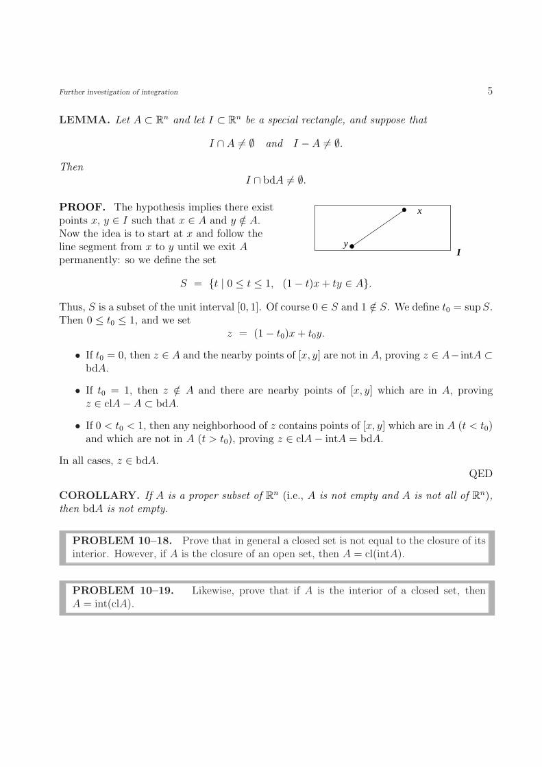
LEMMA. Let A ⊂ Rn and let I ⊂ Rn be a special rectangle, and suppose that
I ∩ A 6= ∅ and I − A 6= ∅.
ThenI ∩ bdA 6= ∅.
PROOF. The hypothesis implies there exist
y
x
I
points x, y ∈ I such that x ∈ A and y /∈ A.Now the idea is to start at x and follow theline segment from x to y until we exit Apermanently: so we define the set
S = {t | 0 ≤ t ≤ 1, (1− t)x + ty ∈ A}.
Thus, S is a subset of the unit interval [0, 1]. Of course 0 ∈ S and 1 /∈ S. We define t0 = sup S.Then 0 ≤ t0 ≤ 1, and we set
z = (1− t0)x + t0y.
• If t0 = 0, then z ∈ A and the nearby points of [x, y] are not in A, proving z ∈ A− intA ⊂bdA.
• If t0 = 1, then z /∈ A and there are nearby points of [x, y] which are in A, provingz ∈ clA− A ⊂ bdA.
• If 0 < t0 < 1, then any neighborhood of z contains points of [x, y] which are in A (t < t0)and which are not in A (t > t0), proving z ∈ clA− intA = bdA.
In all cases, z ∈ bdA.QED
COROLLARY. If A is a proper subset of Rn (i.e., A is not empty and A is not all of Rn),then bdA is not empty.
PROBLEM 10–18. Prove that in general a closed set is not equal to the closure of itsinterior. However, if A is the closure of an open set, then A = cl(intA).
PROBLEM 10–19. Likewise, prove that if A is the interior of a closed set, thenA = int(clA).

6 Chapter 10
B. Topological characterization of contentednessNow we arrive at a tremendous result, showing that the property of a set’s being content can
be expressed in terms of just the boundary of the set. The entire situation can be understoodfrom the following equation.
THEOREM. Let A ⊂ Rn be a bounded set. Then
vol(A) = vol(A) + vol(bdA).
PROOF. This equation will be achieved by proving two inequalities. First, suppose P andQ are elementary polygons such that
P ⊂ A ⊂ Q.
ThenintP ⊂ intA ⊂ clA ⊂ clQ,
and thusbdA ⊂ clQ− intP.
P
Q
Therefore
vol(bdA) ≤ vol(clQ− intP )
= vol(clQ)− vol(intP )
= vol(Q)− vol(P ),
the last equality being due to the fact that the volume of a special rectangle is the same asthe volume of its interior. It simply does not matter whether we use closed or open polygons.Now rearrange the inequality:
vol(Q) ≥ vol(P ) + vol(bdA).

Further investigation of integration 7
As P and Q are arbitrary,
vol(A) ≥ vol(A) + vol(bdA).
The reverse inequality is apparently somewhat more difficult to establish. Suppose thatR is an arbitrary special polygon which contains bdA. Choose a special rectangle such thatR ⊂ I. Using the edges of R we construct a partition of I in such a way that R itself consists
P R
Q
of the union of certain special rectangles belonging to the partition. Thus we may express Ias a nonoverlapping union of the form
I = R ∪N⋃
j=1
Ij,
where each Ij is a special rectangle. The crucial observation to make is that each open rectangleintIj is either entirely contained in A or entirely contained in I − A. For if intIj contained apoint of A and also a point of I − A, the lemma of the preceding section would imply thatintIj would contain a point of bdA, and thus of R.
We conclude that the sets in the partition of I can be grouped into a nonoverlapping unionas follows:
I = R ∪ P ∪Q,
where P and Q are special polygons such that
intP ⊂ A, intQ ⊂ I − A.
Thus
vol(I) = vol(R) + vol(P ) + vol(Q)
= vol(R) + vol(intP ) + vol(intQ)
≤ vol(R) + vol(A) + vol(I − A).

8 Chapter 10
Since the theorem on p. 9–34 implies that
vol(I) = vol(A) + vol(I − A),
we conclude that
vol(A) ≤ vol(R) + vol(A).
Finally, since R is an arbitrary special polygon containing bdA,
vol(A) ≤ vol(bdA) + vol(A).
QED
We have as an immediate corollary the definitive result about contentedness,
THEOREM. A bounded subset of Rn is contented ⇐⇒ its boundary has zero volume.
PROBLEM 10–20. The theorem on p. 9–30 gives a very elementary proof that if Aand B are contented, then so are A ∩B, A ∪B, and A−B. Give a different proof basedon the theorem we have just proved.
REMARK. We have now seen two proofs of the fact that if we deal with the collectionof contented subsets of Rn, then the operations of taking finite intersections, finite unions,and differences produce contented sets. This is described in set theory by saying that thecontented sets form an algebra of subsets of Rn. The one finite set operation we can’t actuallyinclude is that of complementation, but this is only because we require contented sets to bebounded.
C. Integration over more general sets
Up to this point we have been integrating only over special rectangles. It is extremely easyto generalize to integration over arbitrary sets.
DEFINITION. Suppose A is a bounded subset of Rn, and Af−→ R is a bounded function
defined on A. Let I be any special rectangle containing A, and define the new function Ife−→ R
by
fe(x) =
{f(x) if x ∈ A,
0 if x /∈ A.
Further investigation of integration 9
(The notation is intended to suggest that f has been extended to be zero outside of A.) Thenfe is a bounded function on I, and we define
∫
A
f =
∫
I
fe,
∫
A
f =
∫
I
fe.
(It is an easy matter to check that the definition of these new lower and upper integrals isindependent of the choice of I; this same situation appeared also in Section 9H.)
In particular, we can now simply write
∫
A
1 = vol(A),
∫
A
1 = vol(A).
DEFINITION. We say f is integrable over A if these lower and upper integrals are thesame, and we denote their common value as
∫
A
f =
∫
A
f =
∫
A
f.
It is a straightforward task to use this definition effectively, so we will not have to saymuch about it. Here is an example, a generalization of the theorem on p. 9–33:
THEOREM. Let A and B be bounded subsets of Rn, and let f be integrable over B. Then
∫
B
f =
∫
B∩A
f +
∫
B−A
f.
PROOF. Let I be any special rectangle containing B and define fe to be the extension of fobtained by giving it the value zero outside B. Then fe is an integrable function on I. ThenProblem 9–12 implies immediately that
∫
I
fe =
∫
I
fe1B∩A +
∫
I
(fe − fe1B∩A).

10 Chapter 10
But we have the easy observations
fe1B∩A =
{f on B ∩ A
0 outside B ∩ A,
fe − fe1B∩A =
{f on B − A
0 outside B − A.
Thus we conclude respectively
∫
I
fe1B∩A =
∫
B∩A
f,
∫
I
(fe − fe1B∩A) =
∫
B−A
f.
QED
PROBLEM 10–21. Suppose f is integrable over A and B is a contented subset of Rn.Prove that f is integrable over A ∩B.
D. Cavalieri’s principle
This old and famous principle enables us “to find simply and rapidly the volumes of variousgeometric figures.” It’s an immediate consequence of Fubini’s theorem:
PROBLEM 10–22 (Cavalieri). Let A ⊂ Rn be contented, and for each t ∈ R letA(t) be the “slice”
A(t) = {y ∈ Rn−1 | (y, t) ∈ A}(thus A(t) is a bounded subset of Rn−1). Prove that
voln(A) =
∫ ∞
−∞voln−1(A(t))dt =
∫ ∞
−∞voln−1(A(t))dt
(each of these integrals is of course extended only over a finite interval of R, since A(t) isempty for all sufficiently large |t|).
Further investigation of integration 11
PROBLEM 10–23. This is a favorite problem of basic calculus texts. Find the volumeof the intersection of two right circular cylinders in R3 which have the same radius rand whose axes are orthogonal. [You may assume the resulting set has the descriptionx2
1 + x23 ≤ r2, x2
2 + x23 ≤ r2.]
PROBLEM 10–24. Let B be a contented subset of Rn−1, regarded as the subsetRn−1 × {0} of Rn. Let x ∈ Rn, with nth coordinate xn = h > 0. Let C be the cone withbase B and vertex x:
B
C
x
C = {(1− t)y + tx | 0 ≤ t ≤ 1, y ∈ B}.
It is a fact that C is a contented subset of Rn, but you need not prove that. Prove that
voln(C) =1
nvoln−1(B)h.
(The volume of a cone in Rn is equal to 1/n times the altitude times the volume of thebase.)
Later in the present chapter we shall compute the volumes of balls B(x, r) ⊂ Rn for all n.We can actually already compute these, at least in principle. We introduce the following
NOTATION. αn = voln(B(0, 1))
It is an easy task to conclude that
voln(B(x, r)) = αnrn.

12 Chapter 10
PROBLEM 10–25. Use Cavalieri’s principle to complete the following table:
α1 = 2
α2 = π
α3 = ?
α4 = ?
α5 = ?
α6 = ?
PROBLEM 10–26. Calculate the volume in R3 of the intersection of three cylinders:specifically,
vol3({x ∈ R3 | x21 + x2
2 ≤ 1, x21 + x2
3 ≤ 1, x22 + x2
3 ≤ 1}).
PROBLEM 10–27. Calculate the 4-dimensional volume of the set
{x ∈ R4 | x21 + x2
2 + x24 ≤ 1, x2
1 + x23 + x2
4 ≤ 1, x22 + x2
3 + x24 ≤ 1}.
PROBLEM 10–28. Calculate the 4-dimensional volume of the set
{x ∈ R4 | x21 + x2
2 + x24 ≤ 1, x2
1 + x23 + x2
4 ≤ 1}.
PROBLEM 10–29. Calculate the 4-dimensional volume of the set
{x ∈ R4 | x21 + x2
2 ≤ 1, x23 + x2
4 ≤ 1}.

Further investigation of integration 13
PROBLEM 10–30. Calculate the 4-dimensional volume of the set
{x ∈ R4 | x21 + x2
2 + x24 ≤ 1, x2
3 + x24 ≤ 1}.
PROBLEM 10–31. For any dimension n ≥ 1 and any real number a > 0, let
Sn(a) = {x ∈ Rn | 0 ≤ xi for all i and x1 + · · ·+ xn ≤ a}.
Calculate voln(Sn(a)).
PROBLEM 10–32. A favorite calculus “stunt” is this problem: “A ball in R3 has acylindrical hole bored from it, the axis of the cylinder coinciding with a diameter of theball. The set that remains has height h. What is its volume.”
a. Use Cavalieri to calculate the volume.b. Why is this called a stunt?
h

14 Chapter 10
PROBLEM 10–33∗. Generalize Problem 10–32 by assuming that the hole bored outcomes from a right circular cone with axis coinciding with a diameter of the ball:
hl
Calculate the remaining volume as a functionof the altitude h and the slant height `.
PROBLEM 10–34∗. Generalize Problem 10–32 by assuming that the hole bored outis a paraboloid of revolution:
h
Calculate the remaining volume as a function of h.

Further investigation of integration 15
E. Elementary matricesWe are now going to begin the final item of this chapter, the important change of variable
formula for integrals on Rn. We shall first treat the case of linear variable transformations.This will be done in the following section, and in preparation for that we need to present aninteresting feature of n× n matrices which we have not mentioned heretofore.
As is our custom, when we think of a linear relation connecting x and y ∈ Rn, we representour points as column vectors and we write y = Tx, where T is of course an n× n real matrix.We certainly assume that T is invertible (det T 6= 0), as we are going to be interested in aone-to-one correspondence between x and y.
We are particularly interested in two special kinds of what we shall call elementary matrices.In all cases below k and ` stand for fixed integers between 1 and n.
Multiplying. This is any matrix of the following form. Let c 6= 0. Let M be defined by
mii = 1 if i 6= k,
mkk = c,
mij = 0 if i 6= j.
Note that det M = c and that M−1 is also a multiplying matrix with c replaced by c−1.Illustration (k = 1):
c 0 . . . 00 1 . . . 0...
......
0 0 . . . 1
.
Adding. In this case k 6= ` and let c ∈ R. Let the matrix A be defined by
aii = 1,
akl = c,
aij = 0 for all other (i, j).
Note that det A = 1 and that A−1 is another adding matrix, with c replaced by −c. Illustration(k = 1, l = 2):
1 c 0 . . . 00 1 0 . . . 0...
......
...0 0 0 . . . 1
.
Now notice the effect of multiplying a given matrix on the left by these two kinds of elementarymatrices:

16 Chapter 10
Multiplying. MT is the matrix obtained from T by multiplying row k by the number c.
Adding. AT is the matrix obtained from T by adding c times row l to row k.
PROBLEM 10–35. Describe what happens to T when T is multiplied on the right byan elementary matrix.
It is quite amazing at first glance that just these two types of elementary matrices sufficeto generate all invertible matrices, but the proof is easy:
THEOREM. Every invertible matrix can be expressed as a product of elementary matrices.
PROOF. Let T be an arbitrary n×n invertible matrix. We first want to maneuver to obtainthe entry 1 in the (1, 1) position. There are two possibilities. If t11 6= 0, then there exists aunique multiplying matrix M such that MT has the desired property. If t11 = 0, then the factthat T is invertible implies that some ti1 6= 0, and thus there exists an adding matrix A suchthat AT has the desired property. We describe both possibilities by saying that there existsan elementary matrix E such that ET has the form
ET =
1
...
.
Then there exists a sequence of adding matrices Ak such that
An−1An−2 . . . A1ET =
10...
...0
.
By Problem 10–35, another sequence of adding matrices Ak can be found such that
An−1 . . . A1ETA1 . . . An−1 =
1 0 . . . 00...
...0
.
This new matrix we have manufactured contains an invertible (n − 1) × (n − 1) submatrix,to which we can apply the same procedure. This will not disturb the 1 or the 0’s which are

Further investigation of integration 17
displayed above. Therefore, after n stages we arrive at a formula which can be expressedsymbolically as
ErEr−1 . . . E2E1T F1F2 . . . Fs−1Fs = I,
where all the E’s and F ’s are elementary matrices of the two kinds. Multiplying by theirinverses in the correct way produces the formula
T = E−11 E−1
2 . . . E−1r F−1
s . . . F−12 F−1
1 .
Since the inverses are also elementary matrices, the theorem is proved.QED
Before presenting the integration application of this theorem about matrices, we pause topresent an interesting proof of the profound multiplicative property of determinants. Thisfascinating proof is quite different from the proof we gave back in Section 3G.
THEOREM. det(AB) = det A det B.
PROOF. We are of course assuming A and B are n×n matrices. First we dispense with theeasy singular case in which det A = 0. In this case the columns of A are linearly dependent(see p. 3–36). As the columns of AB are themselves linear combinations of the columns ofA, the columns of AB are also linearly dependent. Therefore det(AB) = 0 and the desiredequation holds.
Now assume det A 6= 0. Then we know that A can be expressed as a product of elementarymatrices,
A = E1 . . . Ek.
But each of the two kinds of elementary matrices enjoys the elementary property
det(EC) = det E det C,
as EC results from C by a row operation as described above. Thus we conclude that
det(AB) = det(E1E2 . . . EkB)
= det E1 det(E2 . . . EkB)
...
= det E1 . . . det Ek det B.
Now use B = I to conclude also that
det A = det E1 . . . Ek.
Therefore,det(AB) = det A det B.
QED

18 Chapter 10
PROBLEM 10–36. Prove that the representation produced in the theorem can beachieved with no more than n2 elementary matrices. Why is n2 “obviously” the leastnumber of elementary matrices that can be employed in general?
PROBLEM 10–37. Write out explicitly the representation of 2×2 matrices as productsof elementary matrices.
PROBLEM 10–38. Let T represent a 90◦ rotation:
T =
(0 −11 0
).
Write T as a product of three adding matrices T = E1E2E3, and draw a sketch of theresult of operating step by step on the square J = [0, 1] × [0, 1]. That is, sketch theparallelograms J , E3J , E2E3J , and TJ .
F. Linear changes of variables
In this section we are going to derive and prove a tremendous formula for changing dummyvariables linearly in a Riemann integral over Rn. The key ingredient in this formula will bethe determinant of the matrix which encodes the linear change of variables.
Before we launch into the actual statement and proof, let’s examine a nice special case.Let T be an invertible n× n real matrix, and express T in the usual manner of displaying itscolumns:
T = (t1 t2 . . . tn),
where tj is of course the column vector
tj =
t1j
t2j...
tnj
.
Denote by J the special rectangle in Rn,
J = [0, 1]× · · · × [0, 1].

Further investigation of integration 19
Then we denote by TJ the set resulting from J by multiplying each member of J by T :
TJ = {Tx | x ∈ J}
=
{T
n∑j=1
xj ej | each 0 ≤ xj ≤ 1
}
=
{n∑
j=1
xjtj | each 0 ≤ xj ≤ 1
}.
This set is therefore exactly the n-dimensional parallelogram with vertex 0 and edges t1, . . . , tn;see p. 8–1. We know from our intuitive treatment of volumes in Chapter 8 that
vol(TJ) = | det T |.
That is,
vol(TJ) = | det T | vol(J).
We are now going to prove from integration theory that this formula holds in utter generality,in that J can be replaced by any contented set in Rn. In fact, we shall prove a great dealmore even than this.
Before doing this, we clarify one small point. When one integrates on R1 and makes achange of variable x = −y, one may write in the time-honored way
∫ b
a
f(x)dx = −∫ −b
−a
f(−y)dy.
This is not very convenient for us, as our usual condition a < b produces −a > −b in the“integral” on the right side. Thus we much prefer to write
∫ b
a
f(x)dx =
∫ −a
−b
f(−y)dy.
Notice the two things that occur with this viewpoint: (1) the change of variable y = −xtransforms the interval [a, b] to the interval [−b,−a], and (2) the absolute value of dy/dx isthe correct change of “differential”:
dx = dy.
The above point of view is the convenient one for n-dimensional integration. In fact, it isconvenient to regard the functions we are integrating as defined on all of Rn, but equal to zero

20 Chapter 10
outside some bounded set. Then we simply need not worry about the domain of integration,and we simply write the integral as ∫
Rn
f(x)dx.
Before starting the theorem, a lemma of a rather technical nature needs to be handled. Itwill help us in stating it if we employ a slight abuse of notation. If T is an n× n matrix, letus also denote the associated function from Rn to Rn by the same letter T ; that is, T is thefunction whose value at x ∈ Rn is Tx. (See Problem 2–77 for a discussion of the distinctionthat usually should be made.) As a result, we can write f ◦ T for the composite funciton, thefunction whose value at x is f(Tx).
You will see that virtually all the “hard” work involved in proving the desired result iscontained in the following
LEMMA. Let E be an elementary matrix, and let Rn f−→ Rn be a step function. Then f ◦ Eis integrable, and ∫
Rn
f(y)dy = | det E|∫
Rn
f(Ex)dx.
PROOF. Since step functions are linear combinations of indicator functions of special rect-angles, we may simply assume that f itself is such an indicator function:
f = 1J , where J = [a1, b1]× · · · × [an, bn].
Note that (1J ◦ E)(x) = 1 ⇐⇒ Ex ∈ J ⇐⇒ x ∈ E−1J . Thus we have the simple formula
1J ◦ E = 1E−1J .
We see then that the formula to be proved is∫
Rn
1J = | det E|∫
Rn
1E−1J ;
in other words,vol(J) = | det E|vol(E−1J).
Of course we must also prove that 1E−1J is integrable, i.e., that E−1J is contented.In case E is a multiplying matrix, this is quite simple. As a typical case suppose
E =
a1
. . .
1
, where a < 0.

Further investigation of integration 21
Then
E−1J =
[b1
a,a1
a
]× [a2, b2]× · · · × [an, bn],
so E−1J is itself also a special rectangle, thus contented, and
vol(J)
vol(E−1J)=
b1 − a1
a1
a− b1
a
= −a = | det E|.
The case in which E is an adding matrix has a bit of a twist (really, a shear). As a typicalcase suppose
E =
1. . .
c 1
,
where the nonzero entry c is in the (n, 1) position. Then E−1J is not a rectangle, but is insteaddescribed by noting that x ∈ E−1J ⇐⇒ Ex ∈ J ⇐⇒
a1 ≤ x1 ≤ b1,
...
an−1 ≤ xn−1 ≤ bn−1,
an ≤ cx1 + xn ≤ bn.
The last condition can be rewritten in the form
an − cx1 ≤ xn ≤ bn − cx1,
and E−1J can be represented by a sketch in the x1 − xn plane:
a1
b1
x1
an
bn
an
bn
−ca 1
−ca 1
−cb 1
−cb 1

22 Chapter 10
First, this set is seen as the set contained between the graphs of two functions of x1, . . . , xn−1
(namely, the affine functions an− cx1 and bn− cx1). As these functions are continuous, the setE−1J is contented. This is an application of a slight modification of the theorem of Section 9I.Finally, Cavalieri’s principle gives the required formula for volume. The slice of E−1J for agiven x1 = t, a1 ≤ t ≤ b1, is the special rectangle
[a2, b2]× · · · × [an−1, bn−1]× [an − ct, bn − ct],
and the (n− 1)-dimensional volume of this slice is
(b2 − a2) · · · (bn − an).
Thus Cavalieri gives us
vol(E−1J) =
∫ b1
a1
(b2 − a2) · · · (bn − an)dt
= (b1 − a1)(b2 − a2) · · · (bn − an)
= vol(J).
Since det E = 1, the desired formula is proved.QED
The hard work is over, and it is now a rather soft task to finish what we need to say aboutthe linear case.
THEOREM. Let T be a real n×n matrix with det T 6= 0. Let Rn f−→ R be a bounded functionwhich is zero outside some bounded set. Then
∫
Rn
f(y)dy = | det T |∫
Rn
f(Tx)dx,
and likewise for lower integrals. Moreover, f is integrable ⇐⇒ f ◦ T is integrable, and in thiscase ∫
Rn
f(y)dy = | det T |∫
Rn
f(Tx)dx.
PROOF. The proof divides naturally into two stages. First we assume T = E is anelementary matrix. Then we consider any step function τ ≥ f . Clearly, τ ◦ E ≥ f ◦ E.

Further investigation of integration 23
As we know from the lemma, τ ◦ E is integrable. Thus
| det E|∫
f ◦ E ≤ | det E|∫
τ ◦ E
= | det E|∫
τ ◦ E
=
∫τ (also from the lemma).
Since τ ≥ f is arbitrary, we obtain
| det E|∫
f ◦ E ≤∫
f. ((∗))
That’s only an inequality. But we can employ the trick of replacing f by f ◦ E−1 in (∗):
| det E|∫
f ≤∫
f ◦ E−1.
Another ruse: replace E by E−1 in this inequality, and multiply both sides by | det E|, toobtain ∫
f ≤ | det E|∫
f ◦ E.
This is the reverse of (∗), so the theorem holds for the case of elementary matrices.The second stage of the proof is just the observation that if the theorem holds for two
matrices T1 and T2, then it also holds for their product. For
∫f = | det T1|
∫f ◦ T1.
Then use the theorem for the matrix T2 and the function f ◦ T1:
∫f ◦ T1 = | det T2|
∫f ◦ T1 ◦ T2
= | det T2|∫
f ◦ (T1T2).
Since the determinant is multiplicative, these two equations combine to produce
∫f = | det T1T2|
∫f ◦ (T1T2).

24 Chapter 10
Finally, since any T is a product of elementary matrices, and the theorem is valid for elemen-tary matrices, the theorem is valid in general.
QED
PROBLEM 10–39. Prove that if A is any bounded set in Rn,
vol(TA) = | det T | vol(A),
and likewise for lower volumes. Prove that A is contented ⇐⇒ TA is contented and inthis case
vol(TA) = | det T | vol(A).
PROBLEM 10–40. Prove that if Φ ∈ O(n), then
vol(ΦA) = vol(A).
PROBLEM 10–41. Let A be the ellipsoid
x21
a21
+ · · ·+ x2n
a2n
≤ 1,
where the semiaxes a1, . . . , an are any positive numbers. Prove that
vol(A) = αn a1 . . . an.
PROBLEM 10–42. Let M be a symmetric positive definite n × n matrix, and let Abe the ellipsoid defined by
Mx • x ≤ 1.
Prove thatvol(A) =
αn√det M
.
EXAMPLE. Here’s a numerical example which nicely illustrates the power of these linear

Further investigation of integration 25
changes of variables. Let A be the parallelogram in R2 bounded by the four lines
y =x
2− 1 and y =
x
2+ 2,
y = 2x and y = 2x− 1.
Compute ∫∫
A
exdxdy.
We do not even need to draw a sketch(0, −1)
(−2/3, −4/3)
(4/3, 8/3)(2, 3)
of A, but here is one nevertheless:
Now define new dummy variables in a rather obvious way:
{u = y − 2x,
v = y − x2.
This is a linear change of variables, represented as
(uv
)=
(−2 1−1
21
)(xy
).
Notice that the determinant of the displayed matrix is −3/2. The four lines that form A areexpressed in the u− v coordinates as
v = −1 and v = 2,
u = 0 and u = −1, respectively.
Here’s the sketch in the u− v plane:

26 Chapter 10
(−1, −1)
(−1, 2) (0, 2)
(0, −1)
We know that dxdy should become | det T |dudv, but T is really the inverse of the given matrix.Thus, dxdy becomes 2
3dudv. Finally, solving for x gives x = 2
3(v − u). Thus
∫∫
A
exdxdy =
∫ 2
−1
∫ 0
−1
e2(v−u)/3 2
3dudv
=2
3
∫ 2
−1
e2v/3dv ·∫ 0
−1
e−2u/3du
=2
3· 3
2
(e4/3 − e−2/3
) · 3
2
(e2/3 − 1
)
=3
2
(e4/3 − e−2/3
) (e2/3 − 1
).
PROBLEM 10–43. Let A be the parallelogram in the x−y plane with vertices (1,−1),(4, 0), (3, 2), and (0, 1). Compute ∫∫
A
y dxdy.
(Answer: 7/2) Can you now see how to find the area of A by inspection?
PROBLEM 10–44. Let A be the triangular region in the x− y plane determined bythe three lines x− 2y = 1, x + y = 4, and y = 0. Evaluate the integral
∫∫
A
√x + y
x− 2ydxdy
by using the coordinates u = x + y, v = x− 2y.(Answer: 17/9)

Further investigation of integration 27
PROBLEM 10–45. Given n + 1 points p0, p1, . . . , pn in Rn, the simplex determinedby them is the set
S =
{n∑
j=0
tjpj | all tj ≥ 0 andn∑
j=0
tj = 1
}.
Thus a simplex in R1 is an interval, a simplex in R2 is a triangle, and a simplex in R3 isa tetrahedron. Show that S can also be expressed in the form
S =
{p0 +
n∑j=1
tj(pj − p0) | all tj ≥ 0 andn∑
j=1
tj ≤ 1
}.
Using Problem 10–24, show that
vol(S) =1
n!
∣∣ det(p1 − p0 p2 − p0 · · · pn − p0)∣∣ .
(Each pj is written as a column vector.)
PROBLEM 10–46. Show that the result of the preceding problem can also be ex-pressed as an (n + 1)× (n + 1) determinant:
vol(S) =1
n!
∣∣∣∣ det
(p0 p1 . . . pn
1 1 1
) ∣∣∣∣ .
G. The general formula for change of variables
The purpose of the present section is the understanding of the nonlinear generalization ofthe change of variables formula of the preceding section. This is one of the truly great resultsof calculus. It is the final tool which we need in order to make us adept at handling integralsin several variables.
Important as it is, we choose to omit the proof. There are several reasons for this choice.First, knowing the proof will not help us at all in applying the result. Second, the contextfor providing an efficient proof is Lebesgue, not Riemann, integration. To be sure, we couldgive a proof using Riemann integration, but the technical details which would be requiredare actually far more involved than would be the case if we possessed the tool of Lebesgue

28 Chapter 10
integration; the proof in the Lebesgue context is actually quite elegant. Third, the formulawe are going to present is a very natural guess based on our understanding of the linear case,so much so that the result is quite believable.
Thus our goal is to give a precise statement of the result, to provide several useful examples,and to provide exercises which illustrate the power of the result. We now give the exacthypothesis.
Let A1 and A2 be bounded open contented subsets of Rn, and let
A1Φ−→ A2
be a C1 bijection whose inverse is also of class C1.We shall clearly see in some of the applications how these assumptions might be relaxed
in various ways.
THEOREM. Given the above situation, suppose
A2f−→ R
is integrable. Then f ◦ Φ is also integrable, and∫
A2
f(y)dy =
∫
A1
f(Φ(x)) | det Φ′(x) | dx.
In this formula Φ′(x) is the Jacobian matrix defined in Section 2H.
REMARKS. The determinant of the Jacobian matrix of Φ is often called the Jacobiandeterminant of Φ. Notice that in the case of a linear function y = Tx, the Jacobian determi-nant is det T . If we employ a sort of loose notation, regarding Φ as representing y1, . . . , yn asfunctions of x1, . . . , xn, then the Jacobian determinant is precisely
det
∂y1
∂x1. . . ∂y1
∂xn...
...∂yn
∂x1. . . ∂yn
∂xn
.
Notice also that in the linear case our result is precisely that of the preceding section. Inthat section the factor | det T | served as a type of magnification factor for volumes, as in thetypical formula
vol(TA) = | det T | vol(A)
of Problem 10–39.

Further investigation of integration 29
PROBLEM 10–47. Apply the theorem to the following situation: B ⊂ A1 is acontented set and f is the indicator function on A2 defined by
f(y) = 1 ⇐⇒ Φ−1(y) ∈ B.
Show that the resulting formula is
vol(Φ(B)) =
∫
B
| det Φ′(x)|dx.
As a result of this problem we see that Φ transforms subsets of A1 to subsets of A2 insuch a manner that volumes of the transformed sets are calculated using integration over theinitial set with a sort of local magnification factor | det Φ′(x)|. You should be comfortablewith this generalization of the linear case and should feel that approximating B with specialpolygons and using the continuity of | det Φ′(x)| could reasonably be expected to provide anactual proof.
A 1
A2
B ( )BΦ
Φ
POLAR COORDINATES. This is probably the most important of all examples. We usethe usual formulas for polar coordinates in the x− y plane,
{x = r cos θ,
y = r sin θ.
Here 0 < r < ∞ and θ is restricted to some interval of length 2π. (Since r > 0 we aremissing the origin, and if we think of 0 < θ < 2π we are missing the positive x-axis. These areinconsequential details, as the missing sets have zero two-dimensional volume.) The Jacobian

30 Chapter 10
determinant is
det
(cos θ −r sin θsin θ r cos θ
)= r,
so that when we change variables we replace dxdy by rdrdθ. (Notice the dimensional correct-ness.) Thus ∫∫
f(x, y)dxdy =
∫ 2π
0
∫ ∞
0
f(r cos θ, r sin θ)rdrdθ.
EXAMPLE. We can now give a quick derivation of a recursion formula for αn, the volume ofthe unit ball in Rn. We do this by modifying Cavalieri’s principle to step down two dimensionsat once. Thus
voln(B(0, R)) =
∫
x21+···+x2
n<R2
dx1 · · · dxn
=
∫∫
x21+x2
2<R2
(∫
x23+···+x2
n<R2−x21−x2
2
dx3 · · · dxn
)dx1dx2
=
∫∫
x21+x2
2<R2
voln−2
(B(0,
√R2 − x2
1 − x22
)dx1dx2
=
∫∫
x21+x2
2<R2
αn−2(R2 − x2
1 − x22)
n−22 dx1dx2
polar coordinates=
∫ 2π
0
∫ R
0
αn−2(R2 − r2)
n2−1rdrdθ
= 2παn−2 · 1
−2· (R2 − r2)n/2
n/2
∣∣∣∣r=R
r=0
=2π
nαn−2R
n.
Thus
αn =2π
nαn−2.
We conclude therefore that
αn =
{2πn· 2π
n−2· · · 2π
4π if n is even,
2πn· 2π
n−2· · · 2π
32 if n is odd.

Further investigation of integration 31
In other words,
αn =
πn/2
n2· n−2
2· · · 1 if n is even,
π(n−1)/2
n2· n−2
2· · · 1
2
if n is odd.
THE GAUSSIAN INTEGRAL. We calculated this integral once before, in Section 9G, asan illustration of Fubini’s theorem. We do it again here to illustrate polar coordinates. Again,as in Section 9G, define the number
A =
∫ ∞
0
e−x2
dx.
Then
A2 = A
∫ ∞
0
e−x2
dx
=
∫ ∞
0
Ae−x2
dx
=
∫ ∞
0
(∫ ∞
0
e−y2
dy
)e−x2
dx
=
∫ ∞
0
(∫ ∞
0
e−x2−y2
dy
)dx
Fubini=
∫ ∞
0
∫ ∞
0
e−x2−y2
dvol2
polar coordinates=
∫ π/2
0
∫ ∞
0
e−r2
rdrdθ
=π
2
∫ ∞
0
e−r2
rdr
= −π
4e−r2
∣∣∣∣∞
0
=π
4.
Thus A = 12
√π. This was our second computation of the Gaussian integral. We’ll see a third
in Section H.

32 Chapter 10
SPHERICAL COORDINATES FOR R3. As we discussed in Section 6D, we use
x = r sin ϕ cos θ,
y = r sin ϕ sin θ,
z = r cos ϕ.
Here 0 < r < ∞, 0 < ϕ < π, and 0 < θ < 2π. The Jacobian determinant is (if we use theordering r, ϕ, θ)
det
sin ϕ cos θ r cos ϕ cos θ −r sin ϕ sin θsin ϕ sin θ r cos ϕ sin θ r sin ϕ cos θ
cos ϕ −r sin ϕ 0
.
This can be calculated directly to be r2 sin ϕ. An alternate point of view is that the columnsof the matrix are orthogonal vectors whose lengths are, respectively, 1, r, and r sin ϕ. Thedeterminant is ± the volume of the rectangle with these three sides, and is thus ±r2 sin ϕ. Wedon’t care about the sign in the context of integration, as we use the absolute value. Noticethe dimensional correctness of the formula
dxdydz = r2 sin ϕdrdϕdθ.
As an example we compute again the volume of the unit ball,
α3 =
∫
x2+y2+z2<1
dxdydz
=
∫ 2π
0
∫ π
0
∫ 1
0
r2 sin ϕdrdϕdθ
=
∫ 2π
0
dθ ·∫ π
0
sin ϕdϕ ·∫ 1
0
r2dr
= 2π · 2 · 1
3= 4π/3.
PROBLEM 10–48. The formula for spherical coordinates in R4 is given in Problem 6–16. Show that
dvol4 = r3 sin2 ϕ2 sin ϕ1drdϕ1dϕ2dθ.
Use this formula to recalculate α4.

Further investigation of integration 33
INTEGRATION OF SPHERICALLY SYMMETRIC FUNCTIONS. Our experiencewith R2, R3, and R4 reveals a definite pattern. We could write down spherical coordinates forRn in terms of r and n− 1 angles; these angles are ϕ1, . . . , ϕn−2, and θ. Here each 0 < ϕi < π,while 0 < θ < 2π. These must result in a formula of the form
dvoln = rn−1g(ϕ1, . . . , ϕn−2)drdϕ1 . . . dϕn−2dθ,
where we could calculate g if we wished.
Now suppose Rn f−→ R is spherically symmetric with respect to the origin. This meansthat f(x) depends only on ‖x‖. By abuse of notation we choose to write f(‖x‖). Then theintegration formula becomes
∫
Rn
f(‖x‖)dx1 · · · dxn =
∫ ∞
0
∫ π
0
· · ·∫ π
0
∫ 2π
0
f(r)rn−1gdrdϕ1 . . . dϕn−2dθ.
In this integration we can use Fubini’s theorem to split the r integration and the angle inte-grations. The result is
∫
Rn
f(‖x‖)dx1 · · · dxn = C
∫ ∞
0
f(r)rn−1dr,
where C is a certain constant.
PROBLEM 10–49. Choose a certain example for f in the above formula to concludethat C = nαn. The result is therefore
∫
Rn
f(‖x‖)dx1 · · · dxn = nαn
∫ ∞
0
f(r)rn−1dr.
PROBLEM 10–50. The unit ball B(0, 1) can be inscribed in the cube [−1, 1]× · · · ×[−1, 1]. The ratio of the volume of the ball to that of the cube is 2−nαn. Prove thatthis ratio is a strictly decreasing function of n. Also prove that the ratio tends to zero asn →∞. In fact, prove that lim
n→∞αn = 0.
H. The gamma functionThis section is not actually about changing variables in integrals, but instead is a natural
conclusion to what we have learned about the number αn, the volume of the unit ball in Rn. It

34 Chapter 10
is somewhat clumsy to have to use two different sorts of expressions for αn depending on theparity of n, as we have done in the preceding section. We shall soon derive a single formulathat works for all n.
The key lies in the introduction of a function which elegantly interpolates the factorialfunction, which is itself defined only for nonnegative integers. This function is rather artificiallycalled the gamma function. The Greek letter gamma has no real significance in this context,just as the Greek letter pi in itself has no particular relation to circles.
DEFINITION. The gamma function is the function (0,∞)Γ→ R given by the expression
Γ(a) =
∫ ∞
0
ta−1e−tdt, 0 < a < ∞.
We remark that 0 < Γ(a) < ∞. The defining integral is “improper” at infinity, but theexponential decay gives convergence; also the integral is improper at zero if 0 < a < 1, butcomparison with ta−1 gives convergence.
PROBLEM 10–51. Use an integration by parts to prove that
Γ(a + 1) = aΓ(a).
It is clear that Γ(1) = 1, so that Problem 10–51 implies that
Γ(a + 1) = a! if a = 0, 1, 2, . . . .
Thus we can assert that Γ(a), defined for 0 < a < ∞, interpolates the factorial function(a− 1)!, defined only for a = 1, 2, 3, . . . .
PROBLEM 10–52. Use a change of variable to show that
Γ(a) = 2
∫ ∞
0
x2a−1e−x2
dx.
Conclude that
Γ
(1
2
)=√
π.
The equation for Γ(
12
)is truly fascinating! Just think: a rather natural interpolation of
the factorial function produces such an interesting outcome for the “factorial” of −1/2.

Further investigation of integration 35
Now look at the formula for αn, as given on p. 10–31. If n is even, the denominator is
n
2· n− 2
2· · · 1 =
(n
2
)! = Γ
(n
2+ 1
).
If n is odd, it is instead
n
2· n− 2
2· · · 1
2= Γ
(n
2+ 1
)/Γ
(1
2
)
= Γ(n
2+ 1
)/√π.
Thus in all cases we have the single formula
αn =πn/2
Γ(
n2
+ 1) .
Incidentally, some books write a! = Γ(a + 1) for all −1 < a < ∞. With such a definition,then we have the elegant expression
αn =πn/2
(n/2)!.
Our derivation of this formula for αn was a bit clumsy in one sense: it used induction onn and produced two formulas depending on the parity of n. The following exercise producesαn directly, not relying on induction. It even produces the value for Γ(1/2) as a by-product.

36 Chapter 10
PROBLEM 10–53. Consider the n-dimensional Gaussian function
e−‖x‖2
= e−x21−···−x2
n .
In the following calculations do not worry about the improperness of any of the integrals.(This is in accord with the “conservation of mass” principle given on p. 9–25.)
a. Use Problems 10–49 and 52 to show that∫
Rn
e−‖x‖2
dx = nαnΓ(n/2)/2.
b. Use Fubini’s theorem to show that
∫
Rn
e−‖x‖2
dx =n∏
k=1
∫ ∞
−∞e−x2
kdxk.
c. Combine the preceding formulas to achieve
αn = (Γ(1/2))n/
Γ(n
2+ 1
).
d. Use the case n = 2 to show that Γ(1/2) =√
π, and thus to obtain the desiredformula for αn.
THE BETA FUNCTION. There is another important special function, which is closelyrelated to the gamma function. These functions deserve attention because they appear sooften in applications. Again, the word “beta” has no special significance in this context.Incidentally, the letter B in the definition is to be regarded as an upper case beta.
DEFINITION. The beta function is the function (0,∞) × (0,∞)B−→ R given by the
expression
B(a, b) =
∫ 1
0
ta−1(1− t)b−1dt.

Further investigation of integration 37
PROBLEM 10–54. Prove that the defining integral for B(a, b) is finite if a > 0 andb > 0. Prove that B(b, a) = B(a, b). Also prove that
B(a, b) = 2
∫ π/2
0
sin2a−1 θ cos2b−1 θdθ.
The next exercise gives a truly wonderful calculation of the beta function in terms of thegamma function.
PROBLEM 10–55. Explain the validity of each step in the following calculation (youmay ignore the problems connected with the convergence of the integrals). For any a > 0,b > 0,
Γ(a)Γ(b) =
∫ ∞
0
sa−1e−sds ·∫ ∞
0
tb−1e−tdt
=
∫ ∞
0
∫ ∞
0
sa−1tb−1e−(s+t)dsdt
why?=
∫ ∞
0
∫ ∞
t
(x− t)a−1tb−1e−xdxdt
why?=
∫ ∞
0
∫ x
0
(x− t)a−1tb−1e−xdxdt
why?=
∫ ∞
0
∫ 1
0
(x− xy)a−1(xy)b−1e−xxdydx
why?= Γ(a + b)B(a, b).
Thus we have found the formula
B(a, b) =Γ(a)Γ(b)
Γ(a + b).
Notice from Problem 10–54 the special value B(1/2, 1/2) = π. Setting a = b = 1/2 in theformula we have just derived gives therefore Γ(1/2) =
√π. This marks our third derivation of
the Gaussian integral.
The formula for B enables us to compute many difficult integrals very quickly. It doesn’t

38 Chapter 10
help in computing indefinite integrals such as∫
sin12 θdθ;
these are sometimes called incomplete beta functions. But the complete beta function is merely
∫ π/2
0
sin12 θdθ =1
2B(13/2, 1/2)
=Γ(13/2)Γ(1/2)
2Γ(7)
=112· 9
2· 7
2· 5
2· 3
2· 1
2
√π · √π
2 · 6!
=11 · 7 · 3π
211.
PROBLEM 10–56. Use the trigonometric version of B(a, a) (Problem 10–54) and theformula sin 2θ = 2 sin θ cos θ to derive the duplication formula of Legendre:
Γ(2a) =22a−1
√π
Γ(a)Γ
(a +
1
2
).
PROBLEM 10–57. Use the preceding problem to show that
Γ
(1
4
)Γ
(3
4
)= π
√2.
There is another interesting formula for the gamma function, which we can now deriverather easily. It is based on the familiar representation of the exponential function,
ex = limn→∞
(1 +
x
n
)n
.
Now consider the integral representation of Γ(a), but instead of e−t in the integrand insert thepolynomial (1− t/n)n. The resulting integral that we consider is
Γn =
∫ n
0
ta−1
(1− t
n
)n
dt.

Further investigation of integration 39
Replace t by ns to get
Γn = na
∫ 1
0
sa−1 (1− s)n ds.
This integral can be evaluated explicitly simply by integration by parts n times. We canactually circumvent that by noting
Γn = naB(a, n + 1)
= na Γ(a)Γ(n + 1)
Γ(a + n + 1)
= na Γ(a)n!
(a + n) · · · (a + 1)aΓ(a)
=nan!
(a + n) · · · (a + 1)a.
It is not difficult to show that Γn has the limit Γ(a) as n →∞. Thus we obtain
THEOREM. For 0 < a < ∞,
Γ(a) = limn→∞
nan!
(a + n) · · · (a + 1)a.
To be completely honest, we need to provide a justification of the equation
limn→∞
Γn = Γ(a).
There are several ways to prove this, and here is an ad hoc one that has the advantage ofbeing elementary. First note that
e−x ≥ 1− x for all 0 ≤ x ≤ 1.
Thus
e−t =(e−t/n
)n ≥(
1− t
n
)n
.
Therefore we immediately see that
Γ(a) ≥∫ n
0
ta−1e−tdt
≥∫ n
0
ta−1
(1− t
n
)n
dt
= Γn.

40 Chapter 10
Thus we need to establish some sort of reverse inequality.One such inequality is this:
e−t ≤(
1− t
n
)n
+t
nfor 0 ≤ t ≤ n.
To prove this define
g(t) = et
[(1− t
n
)n
+t
n
].
We need to show that g(t) ≥ 1. Since g(0) = 1, it will suffice to prove that g′(t) ≥ 0. But
g′(t) = et
[(1− t
n
)n
+t
n−
(1− t
n
)n−1
+1
n
]
= et
[t
n
{1−
(1− t
n
)n−1}
+1
n
]
> 0.
Now let ε > 0 be arbitrary, and choose t0 sufficiently large that∫ ∞
t0
ta−1e−tdt ≤ ε.
We conclude that for all n > t0
Γ(a) ≤ ε +
∫ t0
0
ta−1e−tdt
≤ ε +
∫ t0
0
ta−1
(1− t
n
)n
dt +
∫ t0
0
ta−1 t
ndt
≤ ε +
∫ n
0
ta−1
(1− t
n
)n
dt +ta+10
(a + 1)n
= ε +ta+10
(a + 1)n+ Γn.
Therefore, for all sufficiently large n,
Γ(a) < 2ε + Γn.
We conclude that Γn has the limiting value Γ(a).

Further investigation of integration 41
PROBLEM 10–58. Use the above theorem to prove
Wallis’ formula :π
2= lim
n→∞2
1· 2
3· 4
3· 4
5· · · 2n
2n− 1· 2n
2n + 1.
(This is usually writtenπ
2=
2
1· 2
3· 4
3· 4
5· 6
5· 6
7· · · .)
I. Notation for the Jacobian determinantThere is a very fine notational device which aids the memory in handling changes of
variables. Returning to the theorem of Section G, where y = Φ(x) denoted the variablechange, we have the scale factor
det Φ′(x).
The clever notation for this quantity is
∂(y1, . . . , yn)
∂(x1, . . . , xn).
That is,∂(y1, . . . , yn)
∂(x1, . . . , xn)= det(∂yi/∂xj).
With this notation the formula for changing variables looks almost like that of the one-dimensional case (except for the absolute value sign):
∫
y∈A2
f(y)dy =
∫
x∈A1
f(Φ(x))
∣∣∣∣∂(y1, . . . , yn)
∂(x1, . . . , xn)
∣∣∣∣ dx.
PROBLEM 10–59. Show that
∂(x1, . . . , xn)
∂(y1, . . . , yn)= 1
/∂(y1, . . . , yn)
∂(x1, . . . , xn).
EXAMPLE. Let A be the region in the first quadrant of the x− y plane determined by theinequalities x < y < 3x and 2 < xy < 4. For this region we would likely be interested in avariable transformation of the sort

42 Chapter 10
{u = y/x,
v = xy.
Then
y
A
x∂(u, v)
∂(x, y)= det
(−yx−2 x−1
y x
)
= −2y/x.
Notice that we can express x, y explicitly in terms of the new variables as{
x =√
vu,
y =√
uv.
Therefore the change of variables we obtain is
dxdy =x
2ydudv
=1
2ududv,
and we obtain for example∫
A
xdxdy =
∫
1<u<32<v<4
√v
u
1
2ududv
=1
2
∫ 3
1
∫ 4
2
√vu−3/2dvdu
=1
2
∫ 3
1
u−3/2du ·∫ 4
2
√vdv
=1
2· 2
(1− 1√
3
)· 2
3(8− 2
√2)
=4
3
(1− 1√
3
)(4−
√2).
PROBLEM 10–60. Calculate the area of the set A in the preceding problem.(Answer: log 3)

Further investigation of integration 43
PROBLEM 10–61. For 2 × 2 matrices A regard det A as a function from R4 to R,and then calculate
a. the average of | det A| over the cube [0, 1]4;
b. the average of | det A| over the cube [−1, 1]4.
(Answers: 13/54 and 10/27)
PROBLEM 10–62. Repeat the preceding problem, only with | det A| replaced with(det A)2.(Answers: 7/72 and 2/9)
PROBLEM 10–63. For 3 × 3 matrices A regard det A as a function from R9 to R,and then calculate
a. the average of (det A)2 over the cube [0, 1]9;
b. the average of (det A)2 over the cube [−1, 1]9.
(Answers: 5/144 and 1/9)
My student Stefan Allan recently showed me a problem from page 187 of Niven, Zuckerman,and Montgomery, An Introduction to the Theory of Numbers, 5th edition, 1991, and thefollowing problem is based on that one.
PROBLEM 10–64. The floor function defined on R is defined by the expression
btc = largest integer less than or equal to t.
(Sometimes this is designated [t].) Let a ∈ Rn have integer coordinates, and evaluate theintegral ∫
[0,1]nba • xcdx.
(HINT: change variables with xi = 1− yi.)

44 Chapter 10
PROBLEM 10–65. Under the same conditions as in the preceding problem, showthat ∫
[−1,1]nba • xcdx = −1.