fuzzy-stochasticpartialdifferentialequations · fuzzy-stochasticpartialdifferentialequations...
TRANSCRIPT

Fuzzy-Stochastic Partial Differential EquationsMohammad Motamed∗1
1Department of Mathematics and Statistics, The University of New Mexico, Albuquerque, USA
June 5, 2018
Abstract
We introduce and study a new class of partial differential equations (PDEs) with hybridfuzzy-stochastic parameters, coined fuzzy-stochastic PDEs. Compared to purely stochas-tic PDEs or purely fuzzy PDEs, which may treat either only random or only non-randomuncertainty in physical systems, fuzzy-stochastic PDEs offer powerful models for accurate de-scription and propagation of the hybrid random and non-random uncertainties inevitable inmany real applications. We will use the level-set representation of fuzzy functions and definethe solution to fuzzy-stochastic PDE problems through a corresponding parametric problem,and further present theoretical results on the well-posedness and regularity of such problems.We also propose a numerical strategy for computing output fuzzy-stochastic quantities, suchas fuzzy failure probabilities and fuzzy probability distributions. We present two numericalexamples to compute various fuzzy-stochastic quantities and to demonstrate the applicabilityof fuzzy-stochastic PDEs to complex engineering problems.
1 Introduction
Most viable uncertainty quantification (UQ) methodologies are set in a probabilistic framework;see e.g. [50, 7, 24, 55], where the underlying mathematical models are often PDEs with stochasticparameters. In such a framework, the forward propagation of uncertainty is often performed byMonte Carlo sampling techniques [21, 15, 27, 26, 37] or spectral stochastic techniques [9, 56, 38],and the inverse propagation of uncertainty is done by Bayesian inference [29, 49, 23]. All theseapproaches assume that the uncertainty in the model parameters is precisely known and can bedescribed by precise probability distribution functions (PDFs). They are therefore suitable fortreating aleatoric (or random) uncertainty, which arises from inherent randomness or variabilityin a system. There is yet another type of uncertainty, known as epistemic (or non-random)uncertainty, that arises from limited and/or inaccurate information about a system, for instancefrom insufficient data or an inaccurate model. It does not have a random nature and may not beaccurately described by precise PDFs [53, 14]. One approach to represent non-random epistemicuncertainty is through interval analysis [36]. In this approach uncertain parameters are representedby closed intervals describing the incomplete knowledge of parameters. Another approach that
1
arX
iv:1
706.
0053
8v2
[m
ath.
AP]
2 J
un 2
018

generalizes interval analysis lies within the framework of fuzzy set theory [60]. In a fuzzy setelements can partially be in the set. This notion can be exploited to represent an epistemicallyuncertain parameter by a set of nested intervals with different membership degrees. In a fuzzyframework the underlying mathematical models are often PDEs with fuzzy parameters; see e.g.[12, 16, 10]. Solving fuzzy PDEs leads to fuzzy computations that involve interval arithmetic[28, 36] and optimization [31, 40] at different membership levels.
Many real-world problems indeed exhibit a mixture of aleatoric and epistemic uncertainties. Atypical example is the dynamic response of composite materials, such as carbon fiber polymers,where uncertainty in material properties and damage parameters has contributions from both types[3]. On the one hand, variations in material properties (such as the modulus of elasticity) andthe spatial distribution of fiber constituents are of random nature. On the other hand, mate-rial constants may be either difficult or impossible to measure. Moreover, materials may comefrom different manufacturers, and there may be large variations in their quality leading to largevariations in the experimental measurements. When experiments cannot be performed, materialconstants must be obtained from the literature, such as handbooks and standards. There may belarge disagreement in the literature for the values of these quantities. For example, see [8] thatstudies large variations in the thermal conductivity of stainless steel AISI 304, based on the datagiven in various sources [1, 51]. Such experimental and literature-based variations, which may belarger than the intrinsic random experimental noise, will introduce epistemic uncertainty.
A major difficulty that arises in modeling uncertainty in real-world problems is that thereis often no clear-cut distinction between aleatoric and epistemic uncertainty. There may be arandom quantity whose parameters are partially known, or there may be an epistemically uncertainquantity for which some values are more likely to occur than others. Consequently, it may notbe possible to simply model aleatoric uncertainty by probability distributions and epistemic oneby intervals or fuzzy sets. In such situations a hybrid model obtained by the synthesis of the twomodels, rather than simply adding them, is needed to model hybrid uncertainties.
One approach to describe hybrid uncertainties is to synthetize interval analysis and probabilitytheory and build up interval-valued probability distributions [54]. This approach constructs aprobability-box (or a p-box) consisting of a family of cumulative distribution functions (CDFs).The left and right envelopes of the family will form a box and bound the “unknown” distributionof the uncertain parameter from above and below. We also refer to a recent approach, knownas optimal UQ [42], where the optimal distribution among the family is targeted and obtainedas the candidate for the “unknown” distribution. Other related approaches in the framework ofimprecise probability include coherent lower and upper previsions [52], second-order hierarchicalprobabilities [23], and the Dempster-Shafer theory of beleif functions [47]. Another approach thatgoes beyond the framework of probability is to synthesize probability theory and fuzzy set theory,thereby building fuzzy probability distributions [62, 35, 11, 17]. We refer to [53, 19] for a generaldiscussion of the subject.
In the present work we consider the hybrid fuzzy-probability approach to UQ, and introduceand study PDEs with fuzzy-stochastic parameters. Such hybrid PDEs will serve as the underlyingmathematical models for physical systems subject to hybrid random and non-random uncertainties.Compared to purely stochastic PDEs and purely fuzzy PDEs, which may treat either only randomand only non-random uncertainty in physical systems, respectively, fuzzy-stochastic PDEs offerpowerful tools and models for accurate description and propagation of hybrid uncertainties. We
2

use the level-set representation of fuzzy functions and define the solution to a fuzzy-stochastic PDEproblem through a corresponding parametric problem, and further develop theoretical results onthe existence, uniqueness, and regularity of the solution. We then present a numerical approachfor computing fuzzy-stochastic quantities, such as fuzzy failure probabilities and fuzzy probabilitydistributions. Considering the notion of full interaction between fuzzy variables and incorporatingit in the proposed numerical approach, we avoid overestimating the lower and upper bounds ofoutput intervals, a problem known as dependency phenomenon [36] that may occur in intervalarithmetic and fuzzy computations. We present two numerical examples. In the first example,we will compute and visualize various types of fuzzy-stochastic quantities of interest (QoIs) beingfunctionals of the PDE solution. In the second example, we will demonstrate the importanceand applicability of fuzzy-stochastic PDEs for an engineering problem in materials science: theresponse of fiber-reinforced polymers to external forces.
The main contributions of this paper include: 1) introducing fuzzy-stochastic PDEs and defin-ing their solution; 2) presenting rigorous well-posedness and regularity analysis of such PDEs; and3) developing a numerical algorithm for computing fuzzy-stochastic quantities, taking into accountthe full interaction between fuzzy variables. The development of more efficient numerical methodsfor solving fuzzy-stochastic PDEs and more sophisticated numerical experiments are the subjectsof our current work and will be presented elsewhere.
The rest of the paper is organized as follows. Section 2 provides the mathematical and com-putational foundations of fuzzy and fuzzy-stochastic quantities necessary for and relevant to thefocus of this work. In Section 3 we present fuzzy-stochastic PDEs and define their solution. Thewell-posedness and regularity of the fuzzy-stochastic problems are discussed in Section 4. Wepresent two numerical examples in Section 5.
2 Fuzzy and Fuzzy-Stochastic Quantities
This section provides the mathematical and computational foundations of fuzzy and fuzzy-stochasticquantities. Only the concepts relevant to the focus of this work are discussed here. We refer to[18, 30, 44, 35, 11, 17] for a more general description of fuzzy set theory and fuzzy randomnessfrom an engineering point of view.
2.1 Fuzzy variables
Fuzzy sets [60], or fuzzy variables, generalize the notion of crisp sets. In a crisp set, the membershipof an element is given by the characteristic function, taking values either 0 (not a member) or 1 (amember). In a fuzzy set, elements can partially be in the set. Each element is given a membershipdegree, ranging from 0 to 1; see Figure 1.
Definition 1. A fuzzy variable is defined by a set of pairs
z = (z, µz(z)), z ∈ Z ⊂ R, µz : Z → [0, 1],
where Z, referred to as the universe, is a non-empty subset of the real line R, and µz is a member-ship function defined on Z with range [0, 1]. The set of all fuzzy variables defined on Z is denotedby F(Z).
3

crisp set
0 1
0 1
fuzzy set
mem
bers
hip
valu
e
z µ
Figure 1: The notion of membership in crisp sets and fuzzy sets.
It is to be noted that in general the range of the membership function may be the subset ofnonnegative real numbers whose supremum is finite. However, it is always possible to normalizethe range to [0, 1]. Such fuzzy variables, considered here, are sometimes referred to as normalizedfuzzy variables. Throughout the present paper, a (normalized) fuzzy variable is denoted by thesuperimposition of a tilde over a letter.
An important notion in fuzzy set theory is the notion of α-cuts (see e.g. [18, 30]), which allowsone to decompose fuzzy computations into several interval computations.
Definition 2. Any membership function µz of a fuzzy variable z ∈ F(Z) can be represented by afamily S zα ⊂ Z, α ∈ [0, 1] of its α-level sets, known as α-cuts:
S z0 = closurez ∈ Z |µz(z) > 0, and S zα = z ∈ Z |µz(z) ≥ α, ∀α ∈ (0, 1].
In the present work we will need the following assumptions:
(A1) The universe Z ⊂ R is a bounded, convex set.
(A2) The membershipf function is upper semicontinuous, i.e.
lim supz→z0
µz(z) ≤ µz(z0), ∀z0 ∈ Z.
(A3) The membership function is quasi-concave, i.e.
µz(λ z1 + (1− λ) z2) ≥ min(µz(z1), µz(z2)), ∀ z1, z2 ∈ Z, ∀λ ∈ [0, 1].
The boundedness of Z in (A1) implies that the α-cuts are bounded sets. This assumption isnatural for the physical quantities to be represented by fuzzy variables, as such quantities areusually bounded. The convexity of Z in (A1) ensures that ∀z1, z2 ∈ Z and ∀λ ∈ [0, 1], we haveλ z1 + (1− λ) z2 ∈ Z, which is needed for (A3). Assumptions (A2)-(A3) imply that the α-cuts areclosed and convex sets, respectively. Hence, for a fuzzy variable z ∈ F(Z) satisfying assumptions(A1)-(A3), the α-cuts S zα will be bounded, closed intervals with the inclusion property S zα2 ⊂ S zα1
for 0 ≤ α1 ≤ α2 ≤ 1; see Figure 2.We also define the following relational operators for fuzzy variables (see e.g. [18]), needed for
the boundedness and positivity assumption (10) needed in Section 3.
4

z µ0 1
0 1
α2
α1
z, µz(z))
S zα1
S zα2
S z0
S z1
Figure 2: The α-cuts of z ∈ F(Z) satisfying (A1)-(A3) are closed, bounded, nested intervals.
Definition 3. A fuzzy variable z ∈ F(Z) is greater than or equal to a real number a if µz(z) = 0,∀z ∈ Z such that z < a. This is denoted by z ≥ a. Similarly, a fuzzy variable z ∈ F(Z) is smallerthan or equal to a real number a if µz(z) = 0, ∀z ∈ Z such that z > a. This is denoted by z ≤ a.
We note that the above relations can also be expressed in terms of the zero-cut. A fuzzy variableis greater (respectively smaller) than a real number if the real number is smaller (respeactivelygreater) than all points on the zero-cut of the fuzzy variable.Fuzzy vectors. A fuzzy vector can be considered as the n-dimensional generalization of a fuzzyvariable, with n ≥ 2.
Definition 4. An n-dimensional fuzzy vector is defined by a set of pairs
z = (z, µz(z)), z ∈ Z ⊂ Rn, µz : Z→ [0, 1],
where the universe Z is a non-empty subset of Rn, and µz is a joint membership function withrange [0, 1]. The set of all fuzzy vectors z on Z is denoted by F(Z).
An fuzzy vector, witten as z = (z1, . . . , zn), is in fact a collection of n fuzzy variables zi =(zi, µzi(zi)), zi ∈ Zi ⊂ R, µzi : Zi → [0, 1], with i = 1, . . . , n. The universe on which thefuzzy vector is defined is a subset of the Cartesian product of the one-dimensional universes, i.e.Z ⊂ Z1 × · · · × Zn.
Analogous to one-dimensional α-cuts we can define α-cuts for fuzzy vectors.
Definition 5. Any joint membership function µz of an n-dimensional fuzzy vector z ∈ F(Z) canbe identified with the one-parametric family S z
α ⊂ Z, α ∈ [0, 1] of n-dimensional joint α-cuts:
S z0 = closurez ∈ Z |µz(z) > 0, and S z
α = z ∈ Z |µz(z) ≥ α, ∀α ∈ (0, 1]. (1)
Similar to the case of fuzzy variables, we will need the following assumptions:
(A4) The universe Z ⊂ Rn is a bounded, convex set.
(A5) The joint membershipf function is upper semicontinuous.
(A6) The joint membership function is quasi-concave.
5

It is to be noted that for a fuzzy vector z ∈ F(Z) satisfying assumptions (A4)-(A6), the jointα-cuts (1) will be compact, convex sets satisfying the inclusion property:
S zα2 ⊂ S z
α1 , 0 ≤ α1 ≤ α2 ≤ 1. (2)
Interaction. In fuzzy arithmetic it is important to consider the interaction between fuzzy variables(analogous to the correlation between random variables). In general, one can distinguish betweenthree types of interaction and split fuzzy variables into three types: 1) non-interactive variables;2) fully interactive variables; and 3) partially interactive variables. Interaction can be defined interms of the notion of α-cuts.
Definition 6. Consider a fuzzy vector z ∈ F(Z) consisting of n ≥ 2 fuzzy variables zi ∈ F(Zi),with i = 1, . . . , n, satisfying (A4)-(A6). Let S ziα be the one-dimensional (or marginal) α-cut intervalcorresponding to each fuzzy variable zi. The fuzzy variables zini=1 are said to be non-interactiveif their joint α-cut S z
α is the n-dimensional hyperrectangle given by the Cartesian product of nmarginal α-cuts:
S zα = S z1
α × . . .× S znα =:n∏i=1
S ziα , ∀α ∈ [0, 1].
Definition 7. The fuzzy variables zini=1 in Definition 6 are said to be fully interactive if theirjoint α-cut S z
α is a (possibly non-linear) continuous curve in the hyperrectangle ∏ni=1 S
ziα ⊂ Rn,
satisfying the inclusion property (2).
It is to be noted that since the joint α-cut S zα of fully interactive fuzzy variables is a continuous
curve in Rn, there is a bijective mapping between S zα and a one-dimensional closed, bounded
interval Iα = [0, Lα] ⊂ R, with Lα being the Euclidean length of the curve S zα. By the arc
length parameterization of the curve we can therefore obtain a (possibly non-linear) bijective mapϕα : [0, Lα] → Rn so that ϕα(s) ∈ S z
α for each arc length parameter s ∈ Iα = [0, Lα]. Suchmapping facilitates practical fuzzy computations; see Section 5.
Clearly, unlike the case of non-interactive fuzzy variables for which the inclusion property (2)is automatically satisfied, in the case of fully-interactive variables the inclusion property mustbe imposed, because not every continuous curve in the hyperrectangle satisfies this property. Aparticular type of full interaction that can be easily handeled in practical computations may beconsidered by setting the joint α-cut to be the polygonal (i.e. continuous and piecewise linear)curve, given recursively by
S z1 = diag(
n∏i=1
S zi1 ),
S zαj
= S zαj+1
⋃diag(
n∏i=1
[S ziαj \ S ziαj+1]l)⋃
diag(n∏i=1
[S ziαj \ S ziαj+1]r), 0 ≤ αj < αj+1 ≤ 1.
Here, diag(∏ni=1 S
i) with Si = [S¯i, Si] denotes the main space diagonal of the hyperrectangle
S = ∏ni=1 S
i, i.e. the line segment between the vertices (S¯
1, . . . , S¯n) and (S1, . . . , Sn), and the
hyperrectangles [S ziαj \S ziαj+1]l and [S ziαj \S ziαj+1
]r are the left and right portions of the set S ziαj \S ziαj+1,
respectively; see Figure 3. We notice that this setting ensures that the inclusion property (2) holds.
6

0 1
0 1
zi
αj
αj+1
1 + 1 + 1! "# $ 1 + 1 + 1! "# $1# $! "1 + 1 + 1
µzi(zi)
S ziαj+1
d [S ziαj
\S ziαj+1
]lz z
and [S ziαj
\S ziαj+1
]r
Figure 3: The intervals used in the definition of the joint α-cuts of fully interactive fuzzy variablesby polygonal nested curves. We have S ziαj = S ziαj+1
⋃ [S ziαj \ S ziαj+1]l⋃ [S ziαj \ S ziαj+1
]r with αj < αj+1.
Definition 8. The fuzzy variables zini=1 in Definition 6 are said to be partially interactive if theyare neither non-interactive nor fully interactive.
Due to the assumptions (A4)-(A6), Definition 8 implies that the joint α-cut S zα of partially
interactive fuzzy variables is a strict subset of the Cartesian product of the marginal α-cuts, thatis, S z
α ( ∏ni=1 S
ziα , ∀α ∈ [0, 1]. Moreover, it cannot be mapped into a one-dimensional interval. In
practice the joint α-cuts of partially interactive variables are geometrically more complicated thanthose of non-interactive and fully interactive variables. Efficient fuzzy computation in the caseof partial interaction is a challenging task due to the need for solving constrained optimizationproblems over complicated joint α-cuts. We refer to [46] for the treatment of particular types ofpartial interaction using triangular norms.
Importantly, partial interaction does not often occur in hybrid fuzzy-stochastic modeling, andhence we may not need to treat this case in a hybrid fuzzy-stochastic framework. Full interactionmay however occur in hybrid fuzzy-stochastic models. An example is when the uncertain parameteris characterized by a random variable with fuzzy statistical moments using a set of measurementdata. Since the moments are directly related to each other, i.e. higher moments are obtained fromlower moments, the fuzzy moments may be fully interactive; see Section 5.2. Another example,which may occur even in a pure fuzzy framework, is when we perform mathematical operationson two functions with the same fuzzy arguments. In this case the two fuzzy functions are fullyinteractive.
Although in a hybrid framework we often face non-interactive and/or fully interactive fuzzyvariables, we note that the mathematical definitions and results in the present paper are inde-pendent of the type of interaction between fuzzy variables. In the rest of the paper whenever thetype of interaction between fuzzy variables is not specified, the fuzzy variables are understood asgeneral fuzzy variables in F(Z).
2.2 Fuzzy functions
A fuzzy function is a generalization of the concept of a classical function. A classical function isa mapping from its domain of definition into its range. There are various generalizations in theliterature on fuzzy calculus; see e.g. [18, 35] and the references therein. Here, we consider onlytwo cases: 1) a crisp map with fuzzy arguments, and 2) a crisp map with both fuzzy and nonfuzzy
7

arguments.
Definition 9. Consider a function u : Z → V mapping every element of its domain Z ⊂ Rn toan element of its range V = v ∈ R| v = u(z), z ∈ Z ⊂ R. Let further z ∈ F(Z) be a fuzzyvector with a joint membership function µz : Z → [0, 1]. A function u of z, referred to as a fuzzyfunction, is then a mapping
u : F(Z)→ F(V ), V = v ∈ R| v = u(z), z ∈ Z ⊂ R,
so that u := u(z) = (v, µu(v)), v ∈ V ∈ F(V ) is a fuzzy variable with the membership functionµu given by the generalized extension principle [13, 22]:
µu(v) =
supz=u−1(v) µz(z) u−1(v) 6= ∅0 u−1(v) = ∅ , ∀v ∈ V. (3)
Here, u−1(v) is the inverse image of v = u(z) ∈ V and ∅ is the empty set.
Crucially, the generalized extension principle (3) uses the general form of the input joint mem-bership function µz and hence is valid for both non-interactive and interactive input fuzzy variables.
Remark 1. This notion of fuzzy functions was originally introduced by Zadeh [60, 61] for non-interactive input fuzzy variables, where µz is given by the minimum of the marginal membershipsµz(z) = min(µz1(z1), . . . , µzn(zn)), ∀z = (z1, . . . , zn) ∈ Z, and the generalized extension principle(3) reduces to Zadeh’s sup-min extension principle. In [18] this type of mapping is called “fuzzyextension of a nonfuzzy function”.
In order to define fuzzy and fuzzy-stochastic fields that appear in the study of fuzzy-stochasticPDEs, we further need to consider crisp maps with both fuzzy and nonfuzzy arguments. We closelyfollow the extension of classical functions to Sobolev space-valued functions that arise in the studyof time-dependent PDEs; see e.g. [20], and extend the notion of fuzzy functions to fuzzy Sobolevspace-valued functions. In the study of time-dependent PDEs, a function u of space x ∈ D ⊂ Rd
and time t ∈ I ⊂ R may be viewed as a function of t taking values in a function space H(D).A mapping u : I → H(D) can then be defined by [u(t)](x) := u(x, t), ∀t ∈ I, ∀x ∈ D. WhenH(D) is a Sobolev space of functions defined on D, the function u is referred to as a “Sobolevspace-valued function”. This representation is not limited to functions with spatial and temporalarguments and can be generalized to include both fuzzy arguments and nonfuzzy arguments, suchas spatial, temporal, and random variables.
Definition 10. Consider a real-valued function u : X × Z → V mapping every element of itsdomain X×Z, with X ⊂ Rp and Z ⊂ Rn, to an element of its range V = v ∈ R| v = u(κ, z), κ ∈X, z ∈ Z ⊂ R. Let z ∈ F(Z) be a fuzzy vector with a joint membership function µz : Z→ [0, 1].A function u of κ ∈ X and z ∈ F(Z), written as
[u(z)](κ) := u(κ, z), ∀κ ∈ X, z ∈ F(Z), (4)
is defined by an infinite set of fuzzy variables u(κ),κ ∈ X. Each element of this set is a fuzzyvariable u(κ) := [u(z)](κ) corresponding to a fixed κ ∈ X, given by
u(κ) = (v, µu(κ)(v)
), v ∈ V (κ), V (κ) = v = u(κ, z), z ∈ Z ⊂ R, ∀κ ∈ X,
8

with the membership function µu(κ) given by the generalized extension principle (3). The restrictionof (4) to Z is a function of z ∈ Z taking values in a function space H(X), i.e. u : Z → H(X).If H(X) is a Sobolev space, the function (4) may then be viewed as a fuzzy function taking valuesin a Sobolev space. We call such a funcation a fuzzy Sobolev space-valued function, denoted by themapping u : F(Z)→ F(H(X)).
It is to be noted that the function space H may in general be of any type. The main reasonthat we consider Sobolev spaces here is that in the present work such fuzzy functions appear asthe coefficients, data, and solutions to PDE problems.
Remark 2. A fuzzy Sobolev space-valued function is closely related to a fuzzy map with nonfuzzyarguments discussed in [35]. A fuzzy mapping on the nonfuzzy variables κ, denoted by u(κ),may be formulated as a crisp mapping u(κ, z) on the nonfuzzy variables κ and a fuzzy vector zreferred to as “fuzzy bunch parameters”, i.e. u(κ) = u(κ, z). In [35] this is called the bunchparameter respresentation of fuzzy functions. Fuzzy Sobolev space-valued functions are also relatedto “fuzzifying functions” discussed in [18].
Computation of fuzzy functions. The computation of a fuzzy function u amounts to thecomputation of its output membership function µu. Computing µu(v) for all v = u(z) ∈ Vby a direct application of the generalized extension principle (3) can be quite complicated andnumerically cumbersome, as there is no efficient method to evaluate the supremum of µz(z) overall z for which u(z) = v. The computations can substantially be simplified using the α-cutrepresentation of µu, thanks to the following important result, referred to as the function-setidentity [13, 22], extending the earlier work of Nguyen [41].
Theorem 1. (Function-set identity [13, 22]) Let z ∈ F(Z) be a fuzzy vector with a joint mem-bership function µz : Z → [0, 1] and corresponding joint α-cuts S z
α, satisfying the assumptions(A4)-(A6). Let further u : Z→ V be a continuous map, where V = v ∈ R| v = u(z), z ∈ Z ⊂ R.Then the α-cuts Suα corresponding to the output membership function µu of the fuzzy functionu = u(z) ∈ F(V ) is given by:
Suα = u(S zα) = [min
z∈Szα
u(z), maxz∈Sz
α
u(z)], ∀α ∈ [0, 1]. (5)
It is to be noted that two conditions must be satisfied for (5) to hold: 1) the map u : Z →V is continuous, and 2) the fuzzy input vector z ∈ F(Z) satisfies the assumptions (A4)-(A6).Under these two conditions, the α-cuts Suα will be compact intervals given by (5). The continuityassumption holds when, for instance, the function u is the solution to a differential equation underappropriate assumptions on the data. This important observation will be later utilized for theanalysis and computation of fuzzy-stochastic PDEs in this paper.
Crucially, Theorem 1 allows us to decompose fuzzy computations into several interval computa-tions. Motivated by this, we present a numerical approach, outlined in Algorithm 1, for computingfuzzy functions.
The optimization problems in step 2 can be numerically solved for instance by iterative methods;see e.g. [31, 40, 45, 46]. The choice of the method would depend on the dimension and thecomplexity of S z
α and the regularity of u with respect to z.Similarly, the output membership function of a fuzzy Sobolve space-valued function (see Defi-
nition 10) may be computed by Algorithm 1 pointwise in κ ∈ X.
9

Algorithm 1 Computation of fuzzy functions
0. Given a fuzzy vector z ∈ F(Z) satisfying (A4)-(A6) and a continuous map u : Z→ V , whereV = v ∈ R| v = u(z), z ∈ Z ⊂ R, the output membership function of the fuzzy functionu = u(z) ∈ F(V ) is computed as follows.1. Interaction: Find the input joint α-cut S z
α for a fixed α ∈ [0, 1] based on the interactionbetween the input fuzzy variables.2. Optimization: Obtain the output α-cut Suα = [u
¯, u] by computing two global optimization
problems: u¯
:= minz∈Sz
α
u(z) and u := maxz∈Sz
α
u(z).3. Repeat steps 1-2 for various α and form the output membership function µu.
2.3 Fuzzy fields
A scalar fuzzy field is a particular type of a fuzzy Sobolev space-valued function. It is a crisp mapwith spatial variables and a fuzzy vector as arguments generating an infinite set of fuzzy variables.
Definition 11. Let D ⊂ Rd be a compact spatial domain, with d = 1, 2, 3, and consider a vectorof spatial variables x ∈ D. Let further z ∈ F(Z) be a fuzzy vector on Z ⊂ Rn. A scalar fuzzy field,written as u(x) = u(x, z), ∀x ∈ D, is a fuzzy Sobolev space-valued function u : F(Z)→ F(H(D)),where H(D) is a Sobolev space on D.
A typical example of H(D) in the context of PDEs is the Hilbert space of functions whoseweak derivatives up to order s ≥ 0 are square integrable, denoted by Hs(D).
2.4 Fuzzy-stochastic variables
A fuzzy-stochastic variable, introduced in [32, 33], is a generalization of a random variable; see also[62, 35, 11, 17]. Let (Ω,Σ, P ) be a probability space, where Ω is a sample space, Σ is a non-emptysigma-field on Ω, and P is a probability measure assigned to each measurable subset of Ω andsatisfying Kolmogorov’s axioms [25]. A random variable y : Ω → R is a real-valued measurablefunction defined on (Ω,Σ, P ). Every realization of a random variable y(ω), for some ω ∈ Ω, is areal number. If the probability measure P is absolutely continuous [25], it can be described by asingle CDF denoted by F , or a single PDF denoted by π,
F (y0) = P (y ≤ y0) =∫ y0
−∞π(τ) dτ, y0 ∈ R.
The CDF and PDF are usually presented as functions of y0 ∈ R and a set of n crisp parameterscollected in a parameter vector θ ∈ Rn:
F (y0;θ) =∫ y0
−∞π(τ ;θ) dτ, y0 ∈ R, θ ∈ Rn. (6)
For instance, for a normal random variable y ∼ N (θ1, θ22) with two parameters (θ1, θ2) being the
mean and standard deviation, a parameterized CDF is specified as
F (y0;θ) = 1√2πθ2
∫ y0
−∞e
−(τ−θ1)2
2 θ22 dτ, y0 ∈ R, θ = (θ1, θ2) ∈ R2.
This concept can be generalized to define fuzzy-stochastic variables as follows.
10

Definition 12. A fuzzy-stochastic variable y : Ω→ F(V ), with V ⊂ R, is a fuzzy-valued measur-able function on a sample space Ω. Every realization of a fuzzy-stochastic variable y(ω), for someω ∈ Ω, is a fuzzy variable, rather than a real number, given by a set of pairs
y(ω) = (y(ω), µy(y(ω))), y(ω) ∈ V ⊂ R, µy : V → [0, 1], ∀ω ∈ Ω.
The fuzzy-valued probability measure P corresponding to y is described by a fuzzy CDF, denotedby F , and defined in Definition 13 and Definition 15.
We consider and define fuzzy CDFs for two types of fuzzy-stochastic variables:
Type I: random variables with fuzzy parameters;
Type II: outputs of crisp functions with input random and fuzzy variables.
We note that the first type is a special case of the second type. We will first define the notionof fuzzy CDFs for type-I fuzzy-stochastic variables. The definition of fuzzy CDFs for type-IIfuzzy-stochastic variables will be presented in Section 2.5.
Definition 13. (Type-I fuzzy CDF) Consider a type-I fuzzy-stochastic variable y, consisting of arandom variable with n fuzzy parameters θ ∈ F(Z), where Z ⊂ Rn. Let S θα ⊂ Rn be the joint α-cutof θ. For every fixed θ ∈ S θα, let the parameterized CDF of the corresponding random variable begiven by (6). Consider the family of all parameterized CDFs (6) over S θα for a fixed y0 ∈ R:
F (y0;θ), θ ∈ S θα, y0 ∈ R.
At any fixed α-level, let FLα and FR
α be the extrema of the family of parameterized CDFs over thejoint α-cut S θα, referred to as the left (upper) and right (lower) bounds:
FLα (y0) = max
θ∈Sθα
F (y0;θ), FRα (y0) = min
θ∈Sθα
F (y0;θ), ∀α ∈ [0, 1]. (7)
The fuzzy CDF of y, evaluated at y0 ∈ R and denoted by F (y0) = F (y0; θ), is then defined by anested set of left and right bounds at different α-levels:
F (y0) = F (y0; θ) =(FLα (y0), FR
α (y0)), α ∈ [0, 1]
.
Interpretation of fuzzy CDFs. For any fixed α-level, the set of all left and right bounds (7)corresponding to all points y0 will constitute two left and right envelopes forming a p-box. It isimportant to note that the left and right envelopes are not necessarily two single CDFs. In fact, fordifferent values of y0 ∈ R, there may exist different maximizers and/or minimizers. Hence, differentdistributions on different regions may constitute the two envelopes. Fuzzy CDFs provide a far morecomprehensive representation of uncertainty, compared to a class of imprecise probabilistic modelssuch as p-boxes [54], coherent lower and upper previsions [52, 53], and optimal UQ [42] whichprovide only crisp lower and upper bounds from a set of admissible distributions. A fuzzy CDFcan indeed be thought of as a nested set of p-boxes at different levels of possibility (correspondingto different α-levels); see the numerical examples in Section 5.
11
2.5 Fuzzy-stochastic functions
A fuzzy-stochastic function is a particular type of a fuzzy Sobolev space-valued function. It isa crisp map with a random vector and a fuzzy vector as arguments generating an output fuzzy-stochastic variable.
Definition 14. Let y ∈ Γ ⊂ Rm be a random vector and z ∈ F(Z) be a fuzzy vector on Z ⊂ Rn.A fuzzy-stochastic function, written as u(y) = u(y, z), ∀y ∈ Γ, is a fuzzy Sobolev space-valuedfunction u : F(Z)→ F(H(Γ)), with H(Γ) being a Sobolev space of random functions. The fuzzy-valued probability measure P corresponding to u is described by a type-II fuzzy CDF F defined inDefinition 15.
A typical example of H(Γ) is the space of random functions with bounded second moments,denoted by L2
π(Γ).
Definition 15. (Type-II fuzzy CDF) Consider a type-II fuzzy-stochastic variable u, being the out-put of a fuzzy-stochastic function defined in Definition 14. For every fixed z ∈ S z
α, the parameterizedCDF of the corresponding random variable, evaluated at any point u0 ∈ R, will be determined bythe PDF of the input random vector π = π(y) as
F (u0; z) =∫τ :u(τ ,z)≤u0
π(τ ) dτ .
At any fixed α-level, let FLα and FR
α be the extrema of the family of parameterized CDFs over thejoint α-cut S z
α:
FLα (u0) = max
z∈Szα
F (y0; z), FRα (u0) = min
z∈Szα
F (u0; z), ∀α ∈ [0, 1].
The fuzzy CDF of u, evaluated at u0 ∈ R and denoted by F (u0) = F (u0; z), is then defined by anested set of left and right bounds at different α-levels:
F (u0) = F (u0; z) =(FLα (u0), FR
α (u0)), ∀α ∈ [0, 1]
.
Computation of fuzzy-stochastic functions. Let u(y) = u(y, z) be a fuzzy-stochastic func-tion. Assume that we want to compute a fuzzy QoI, denoted by Q, given in terms of u(y). Threeimportant examples of Q include:
• Q = E[ur(y, z)]: the r-th fuzzy moment of u(y), where r is a positive integer.
• Q = F (u0) = E[I[u(y,z)≤u0]]: the fuzzy CDF of u(y) evaluated at a fixed point u0 ∈ R, where I[·]is the indicator function taking the value 1 or 0 if the event [·] is “true” or “false”, respectively.
• Q = E[I[g(u(y,z))≤0]]: the fuzzy failure probability assuming that failure occurs when g(u(y)) ≤ 0,where g is a differential and/or integral operator on u(y).
Each of the above fuzzy QoIs is the expectation of a fuzzy-stochastic function, say Q = E[q(y, z)],where q = ur(y, z) in the first example, q = I[u(y,z)≤u0] in the second example, and q = I[g(u(y,z))≤0]in the third example above. Algorithm 2 outlines a numerical approach for computing Q.
12

Algorithm 2 Computation of fuzzy-stochastic functions
0. Given a random vector y ∈ Γ, a fuzzy vector z ∈ F(Z) satisfying (A4)-(A6), and a fuzzy-stochastic function q : F(Z) → F(H(Γ)), we compute the fuzzy QoI Q = Q(z) = E[q(y, z)] asfollows.1. Interaction: For a fixed α ∈ [0, 1], find the input joint α-cut S z
α based on the interactionbetween the input fuzzy variables.2. Optimization: Obtain the lower and upper bounds of the output α-cut SQα by computing twoglobal optimization problems:
Q¯
:= minz∈Sz
α
Q(z), Q := maxz∈Sz
α
Q(z), Q(z) = E[q(y, z)].
An iterative optimization algorithm requires Mf function evaluations Q(z(k)) at Mf fixed pointsz(k)Mf
k=1 ∈ S zα. Each function evaluation amounts to computing the expectation E[q(y, z(k))]
which may be done by a Monte Carlo sampling strategy or a spectral stochastic method, de-pending on the regularity of q with respect to y.3. Repeat steps 1-2 for various levels of α ∈ [0, 1].
2.6 Fuzzy-stochastic fields
Since the solution of fuzzy-stochastic PDEs are functions of space/time, in addition to beingfunctions of stochastic and fuzzy vectors, the notion of fuzzy-stochastic functions needs to beextended to include the dependency on space/time. A scalar fuzzy-stochastic field is indeed aparticular type of a fuzzy Sobolev space-valued function with a vector of spatial variables, arandom vector, and a fuzzy vector as arguments. Similarly, one can include a temporal variableas argument and define fuzzy-stochastic processes.
Definition 16. Let D ⊂ Rd be a compact spatial domain, with d = 1, 2, 3, and consider a vectorof spatial variables x ∈ D. Let further y ∈ Γ and z ∈ F(Z) be a random vector and a fuzzy vector,respectively. A scalar fuzzy-stochastic field, written as u(x,y) = u(x,y, z), ∀x ∈ D, ∀y ∈ Γ, is afuzzy Sobolev space-valued function u : F(Z)→ F(H(D× Γ)), where H(D× Γ) is a Sobolev spaceof functions on D × Γ.
An example of H(D × Γ) in the context of fuzzy-stochastic PDEs is the Sobolev space offunctions formed by the tensor product of two Sobolev spaces Hs(D)⊗ L2
π(Γ).
3 Fuzzy-Stochastic PDEs
In general, we refer to PDEs with fuzzy-stochastic parameters, including coefficients, force terms,and boundary/initial data, as fuzzy-stochastic PDEs. Without loss of generality, in the presentwork, we consider only the case where the PDE coefficient is a fuzzy-stochastic field and assumethat the forcing and data functions are deterministic.
13

3.1 A fuzzy-stochastic elliptic model problem
Let D ⊂ Rd be a bounded, convex, Lipschitz spatial domain, with d = 1, 2, 3. Consider thefollowing fuzzy-stochastic elliptic boundary value problem:
−∇x · (a(x,y, z) ∇xu(x,y, z)) = f(x), (x,y) ∈ D × Γ, z ∈ F(Z),u(x,y, z) = 0, (x,y) ∈ ∂D × Γ, z ∈ F(Z), (8)
where x = (x1, . . . , xd) ∈ D is the vector of spatial variables, y = (y1, . . . , ym) ∈ Γ ⊂ Rm is arandom vector with a bounded joint PDF π = π(y) : Γ → R+, and z = (z1, . . . , zn) ∈ F(Z) is afuzzy vector on Z ⊂ Rn satisfying assumptions (A4)-(A6) and with a family of joint α-cuts S z
α ⊂ Zwith α ∈ [0, 1]. The only source of uncertainty is assumed to be the parameter a characterized by afuzzy-stochastic field a(x,y) = a(x,y, z). This implies that the PDE solution u(x,y) = u(x,y, z)is a fuzzy-stochastic field; see Section 3.2 for the definition of the PDE solution.
We assume that m and n are finite numbers. We further assume
f ∈ L2(D), (9)
0 < amin ≤ a(x,y) ≤ amax <∞, ∀x ∈ D, ∀y ∈ Γ. (10)Assumption (9) states that the forcing function f is square integrable, and assumption (10) statesthat the PDE coefficient at every fixed (x,y) ∈ D × Γ is a uniformly positive and bounded fuzzyvariable in the sense of Definition 3.
3.2 Solution of the fuzzy-stochastic problem
Following Definition 10 and Definition 16, we interpret the solution u(x,y) = u(x,y, z) to (8),under assumptions (9)-(10), as a fuzzy Sobolev space-valued function:
u : F(Z)→ F(H(D × Γ)), where H(D × Γ) = H10 (D)⊗ L2
π(Γ). (11)
Here, the function space H(D×Γ) is formed by the tensor product of two Sobolev spaces: H10 (D)
is the closure of the space of smooth functions with compact support in the Sobolev space offunctions whose first weak derivatives are square integrable; and L2
π(Γ) is the Sobolev space ofrandom functions with bounded second moments.
For the convenience of both analysis and computation, and thanks to the function-set identity(5), which will be shown to hold (see Theorem 2) due to the continuity of the mapping in (11), wewill define the solution to (8) through the corresponding parametric problem:
−∇x · (a(x,y, z) ∇xu(x,y, z)) = f(x), in D × Γ× S zα,
u(x,y, z) = 0, on ∂D × Γ× S zα,
(12)
where, following the assumption (10),
0 < amin ≤ a(x,y, z) ≤ amax <∞, ∀x ∈ D, ∀y ∈ Γ, ∀ z ∈ S zα. (13)
Corresponding to the interpretation (11), we interpret the solution u(x,y, z) to the parametricproblem (12) as a Sobolev space-valued function on S z
α:
u : S zα → H(D × Γ), where H(D × Γ) = H1
0 (D)⊗ L2π(Γ). (14)
14

As we will show in Section 4, the mapping in (14) is continuous and u is uniformly bounded onS zα, i.e. u ∈ L∞(S z
α; H10 (D)⊗L2
π(Γ)). This suggests that we may obtain the α-cuts of the solution(11) to the fuzzy-stochastic problem (8) from the extrema of the solution (14) to the parametricproblem (12) on the input joint α-cuts S z
α:
Suα(x,y) = [minz∈Sz
α
u(x,y, z),maxz∈Sz
α
u(x,y, z)] =: [u¯α
(x,y), uα(x,y)], α ∈ [0, 1]. (15)
Note that the lower and upper limits of the α-cuts in (15) are stochastic fields. We also noticethat the solution u to (12) is α-dependent. However, for ease of notation, we omit the explicitdependence on α when no ambiguity arises.
The interpretation of the solution to fuzzy-stochastic PDE problems through Sobolev space-valued functions, i.e. the mappings (11) and (14), simplifies the analysis of such problems. Indeed,it transforms the original problem into a parametric one, as done in the case of pure stochasticand pure fuzzy PDEs; see e.g. [5, 38, 16]. We can therefore extend the proofs for well-posednessand regularity of deterministic (see e.g. [20]) and stochastic (see e.g. [5, 38, 39]) problems tofuzzy-stochastic problems.
4 Well-posedness and Regularity Analysis
In this section we will address the well-posedness and regularity of the fuzzy-stochastic problem(8) with a forcing function satisfying (9) and a PDE coefficient satisfying (10).
4.1 Well-posedness
We base the well-posedness analysis on the parametric representation (12) of problem (8) andconsider the following weak formulation of problem (12) pointwise in z ∈ S z
α.Weak formulation I. Find u : S z
α → H10 (D)⊗L2
π(Γ) such that ∀z ∈ S zα and for all test functions
v ∈ H10 (D)⊗ L2
π(Γ) the following holds:∫D×Γa(x,y, z)∇xu(x,y, z) · ∇xv(x,y)π(y)dydx =
∫D×Γ
f(x)v(x,y)π(y)dydx. (16)
Such a solution, provided it exists, is referred to as a weak solution to (12).
Theorem 2. Under the assumptions (9) and (13), there exists a unique weak solution u ∈C0(S z
α; H10 (D) ⊗ L2
π(Γ)) to the parametric problem (12). Moreover, the solution depends con-tinuously on the data.
Proof. Thanks to the uniform positivity assumption (13), we have ∀z ∈ S zα:
amin
∫D×Γ|∇xu(x,y, z)|2 π(y) dy dx ≤
∫D×Γ
a(x,y, z) |∇xu(x,y, z)|2 π(y) dy dx,
and hence, using the notation ‖.‖H := ‖.‖H10 (D)⊗L2
π(Γ) for the norm in H10 (D)⊗ L2
π(Γ),
‖u(z)‖2H ≤
1amin
∫D×Γ
a(x,y, z) |∇xu(x,y, z)|2 π(y) dy dx, ∀ z ∈ S zα.
15

Moreover, due to the uniform boundedness assumption (13) and by Hölder inequality,∣∣∣∣∫D×Γ
a(x,y, z) ∇xu(x,y, z) · ∇xv(x,y) π(y) dy dx∣∣∣∣ ≤ amax ‖u(z)‖H ‖v‖H .
Hence, by the Lax-Milgram theorem [20], there is a unique solution u(z) ∈ H10 (D) ⊗ L2
π(Γ) thatsatisfies (16). By setting v = u(z) in (16) and using Hölder and Poincaré inequalities on the righthand side, we obtain ∀z ∈ S z
α,
amin‖u(z)‖2H ≤
∫D×Γ
a(x,y, z) |∇xu(x,y, z)|2 π(y) dy dx
=∫D×Γ
f(x)u(x,y, z) π(y) dy dx
≤ ‖f‖L2(D) ‖u(z)‖L2(D)⊗L2π(Γ) ≤ C ‖f‖L2(D) ‖u(z)‖H ,
where C is the Poincaré constant:
‖u(x,y, z)‖L2(D) ≤ C ‖u(x,y, z)‖H10 (D), ∀y ∈ Γ, ∀ z ∈ S z
α.
This gives the energy estimate
‖u(z)‖H ≤C
amin‖f‖L2(D), ∀ z ∈ S z
α.
Hence, thanks to assumption (13), the mapping u : S zα → H1
0 (D) ⊗ L2π(Γ) is continuous and
uniformly bounded u ∈ L∞(S zα; H1
0 (D)⊗ L2π(Γ)). This completes the proof.
By Theorem 1 and the continuity of the mapping u : S zα → H1
0 (D)⊗ L2π(Γ) by Theorem 2, we
have the function-set identity
Suα(x,y) = u(x,y, S zα), ∀x ∈ D, ∀y ∈ Γ.
The lower and upper limits of the α-cuts of solution (11) to the fuzzy-stochastic problem (8)may then be obtained from the extrema of the solution (14) to the parametric problem (12).In particular, provied the solution u = u(x,y, z) is a continuous function for every fixed point(x,y) ∈ D × Γ, its α-cuts Suα(x,y) will be compact, nested intervals given by (15) and satisfyingSuα2 ⊂ Suα1 with 0 ≤ α1 ≤ α2 ≤ 1. We notice that in the basence of continuity, an α-cut may bethe union of disjoint intervals, and (15) may not hold.
As a corollary of Theorem 2, we have the following result.
Corollary 1. Consider the fuzzy-stochastic PDE problem (8) under the assumptions (9)-(10).There exists a unique solution u ∈ F(H1
0 (D)⊗ L2π(Γ)) that depends continuously on the data.
The compactness and the inclusion property of the α-cuts (15) is crucial for efficient computa-tions in fuzzy space for two reasons. First, it will allow us to restrict fuzzy computations to onlya few α ∈ [0, 1] levels, for example α = 0, 0.25, 0.5, 0.75, 1. After computing Suα for these α values,the output membership function can be constructed by interpolation. Secondly, since the zero-cutS z
0 contains all other α-cuts, i.e., S zα ⊂ S z
0 , ∀α ∈ (0, 1], we will need to construct the responsesurface of the solution u(x,y, .) only over the zero-cut. Hence we solve the parameteric problem(12) over the zero-cut. The response surface of the solution over any desired α-cut may then beobtained by restricting the zero-cut response surface to the desired α-cut.
16

4.2 Parametric regularity
The convergence rate of spectral methods, such as sparse collocation, depends on the regularity ofthe solution to the parametric problem (12) with respect to parameters both in stochastic spaceand in fuzzy space. We will therefore combine the stochastic and fuzzy spaces and let ξ = (y, z)be the parameter vector in the combined stochastic-fuzzy space
Ξ := Γ× S z0 ⊂ RN , N = m+ n,
and study the ξ-regularity of the solution u(x, ξ) to (12). We note that since the solution overany desired α-cut S z
α, with α ∈ [0, 1], can be obtained by restricting the zero-cut solution to thedesired α-cut, we need to consider only the zero-cut S z
0 in Ξ. Indeed, the regularity of the solutionover the zero-cut will determine the regularity of the solution over all other α-cuts.
We view the solution to the parametric problem (12) as a function of ξ ∈ Ξ taking values in aSobolev space H1
0 (D) and study the regularity of the mapping u : Ξ→ H10 (D). In the light of this
interpretation we consider the following weak formulation of problem (12) pointwise in ξ ∈ Ξ.Weak formulation II. Find u : Ξ→ H1
0 (D) such that ∀ξ ∈ Ξ and for all test functions v ∈ H10 (D)
the following holds:B[u, v] = f(v), (17)
B[u, v] :=∫Da(x, ξ) ∇xu(x, ξ) · ∇xv(x) dx, f(v) =
∫Df(x) v(x) dx. (18)
By assumption (13), the bilinear from B in (18) is uniformly coercive and bounded, that is, ∀ξ ∈ Ξ,
|B[u(ξ), u(ξ)]| ≥ amin ‖u(ξ)‖H10 (D), |B[u(ξ), v]| ≤ amax ‖u(ξ)‖H1
0 (D) ‖v‖H10 (D). (19)
Moreover, by assumption (9) and employing Hölder and Poincaré inequalities, the linear functionalf(v) in (18) is bounded in H1
0 (D),
‖f‖H−1(D) = supv∈H1
0 (D)
|f(v)|‖v‖H1
0 (D)≤ ‖f‖L2(D) ‖v‖L2(D)
‖v‖H10 (D)
≤ C ‖f‖L2(D) ≤ ∞. (20)
Hence, by the Lax-Milgram theorem, there exist a unique solution u ∈ L∞(Ξ;H10 (D)).
For regularity analysis we will also need some regularity assumptions on the ξ-regularity ofthe PDE coefficient. Let k = (k1, . . . , kN) ∈ NN be a multi-index with |k| = k1 + . . . + kN andN denoting the set of all non-negative integers including zero. We make the following regularityassumption on the PDE coefficient,
∂|k|ξ a(., ξ) := ∂|k|a(., ξ)
∂k1ξ1 . . . ∂kNξN
∈ L∞(D), 0 ≤ |k| ≤ s, ∀ ξ ∈ Ξ, (21)
where s ∈ N. The assumption (21) states that a has s bounded mixed ξ-derivatives.We now present the main regularity results. First, we state a component-wise result on the
ξi-regularity of the solution for every component of ξ = (ξ1, . . . , ξN).
Theorem 3. For the solution of (12) with the forcing term satisfying (9) and the coefficientsatisfying (13) and (21), we have for i = 1, . . . , N ,
∂kξiu ∈ L∞(Ξ;H10 (D)), k ∈ N, 0 ≤ k ≤ s.
17

Proof. The case k = 0 follows directly from the weak formulation (17)-(18) and the Lax-Milgramtheorem, thanks to (19) and (20). We now let 1 ≤ k ≤ s and k-times differentiate the weakformulation (17) with respect to the parameter ξi and obtain
B[∂kξiu, v] = Fk(v), (22)
where B is the bilinear from given in (18) with u replaced by ∂kξiu, and Fk(v) is a linear functionalof v which reads
Fk(v) := −k∑`=1
(k
`
) ∫D∂`ξia(x, ξ) ∇x∂
k−`ξi
u(x, ξ) · ∇xv(x) dx. (23)
The weak formulation (22)-(23) has a similar form to (17)-(18) with a slightly different right handside. Hence, the existence of the weak solution ∂kξiu, which determines the ξi-regularity of u followsfrom the boundedness of the functional (23) in H1
0 (D), which can easily be shown by induction onk.
We now state the following result on the mixed ξ-derivative of the solution.
Theorem 4. For the solution of the parametric problem (12) with the forcing term satisfying (9)and the coefficient satisfying (13) and (21), we have,
∂|k|ξ u := ∂|k|u
∂k1ξ1 . . . ∂kNξN
∈ L∞(Ξ;H10 (D)), k ∈ NN , 0 ≤ |k| ≤ s.
Proof. The proof is an easy generalization of the previous theorem, following the arguments in theproof of Theorem 6 in [38].
5 Numerical Experiments
In this section we present two numerical examples. In both examples, we consider the followingfuzzy-stochastic elliptic problem:
d
dx
(a(x,y, z) du
dx(x,y, z)
)= 0, x ∈ [0, L], y ∈ Γ, z ∈ F(Z), (24a)
u(0,y, z) = 0, a(L,y, z) dudx
(L,y, z) = 1. (24b)
Here, the source of uncertainty is the parameter a characterized by a fuzzy-stochastic field; see thetwo examples below. The solution to (24) is analytically given by
u(x,y, z) =∫ x
0a−1(ξ,y, z) dξ. (25)
We note that in more complex problems in higher dimensions, the PDE problem needs to bediscretized on the spatial domain by a numerical method. Here, we consider the one-dimensionalproblem (24) and focus on computations in fuzzy-stochastic spaces. More sophisticated numericalexamples will be presented in forthcoming papers.
18
5.1 Numerical example 1
As an illustrative example, we let L = 2 and consider (24) with the fuzzy-stochastic parameter
a(x, y, z) = a1(x) a2(y, z) = (2 + sin(2π x/L)) ez1+y z2 , y ∼ N (0, 1), z = (z1, z2).
Here, a is a fuzzy-stochastic field, given by the product of a deterministic function a1(x) and afuzzy-stochastic function a2(y, z), being a lognormal random variable with a fuzzy mean z1 and afuzzy standard deviation z2, i.e. a2(y, z) ∼ ln N [z1, z
22 ]. We assume that z1 and z2 are triangular
numbers, that is, they have triangular-shaped membership functions, uniquely described by triples〈zli, zmi , zri 〉, where zli < zmi < zri and such that µzi(zli) = µzi(zri ) = 0 and µzi(zmi ) = 1, with i = 1, 2.The marginal α-cuts of the two fuzzy variables are then given by
S z1α = [zl1 + α (zm1 − zl1), zr1 − α (zr1 − zm1 )] =: [aα, bα],
S z2α = [zl2 + α (zm2 − zl2), zr2 − α (zr2 − zm2 )] =: [cα, dα].
We consider two cases of non-interactive and fully interactive fuzzy variables. If z1 and z2 arenon-interactive, following Definition 6, their joint α-cut is
S zα = [aα, bα]× [cα, dα].
If z1 and z2 are fully interactive, following Definition 7, their joint α-cut may be considered to bea piecewise linear curve in R2 with the Euclidean length
Lα =√
(aα − zm1 )2 + (cα − zm2 )2 +√
(bα − zm1 )2 + (dα − zm2 )2 =: L1,α + L2,α,
given by the collection of points
S zα = (z1, z2) = ϕ(s), s ∈ [0, Lα],
with the piecewise linear map
ϕ(s) =
(aα + s|zm1 − aα|/L1,α, cα + s|zm2 − cα|/L1,α) s ∈ [0, L1,α](zm1 + s|bα − zm1 |/L2,α, z
m2 + s|dα − zm2 |/L2,α) s ∈ [L1,α, Lα] .
We consider the following QoIs
Q1 = Q1(z) = E[u(L, y, z)],Q2(x) = Q2(x, z) = E[u(x, y, z)],Q3(y) = Q3(y, z) = u(L, y, z).
These QoIs cover a wide range of fuzzy quantities: Q1 is a fuzzy function; Q2 is a fuzzy field;and Q3 is a fuzzy-stochastic function. We now discuss the computation and visualization of eachquantity in turn, based on Algorithm 1 and Algorithm 2.
The computation of Q1 amounts to computing its α-cuts SQ1α at various levels α ∈ [0, 1]. It
requires evaluating the PDE solution (25) at a fixed point x = L and for Ms realizations y(i)Msi=1
of y ∼ N (0, 1). The solution (25) at x = L and a fixed realization y(i) is the integral of a fuzzy
19

field a−1(ξ, y(i), z), with ξ ∈ [0, L], over a crisp interval [0, L]. We approximate the crisp integralby a quadrature, such as the midpoint rule, and write
u(L, y(i), z) =∫ L
0a−1(ξ, y(i), z) dξ ≈ h
Nh∑j=1
a−1(xj, y(i), z), xj = (j − 12)h, h = L
Nh
.
Following Algorithm 2, we employ the standard Monte Carlo sampling and write
Q1(z) = E[u(L, y(i), z)
]≈ 1Ms
Ms∑i=1
u(L, y(i), z) ≈ h
Ms
Ms∑i=1
Nh∑j=1
a−1(xj, y(i), z).
Note that we can alternatively employ other Monte Carlo sampling strategies [15, 27, 26, 37] orspectral stochastic techniques [57, 9, 56, 38] to approximate the expectation. Finally, followingAlgorithm 1, we perform the addition ofMsNh fuzzy functions a−1(xj, y(i), z), with j = 1, . . . , Nh
and i = 1, . . . ,Ms, to get:
SQ1α =
[minz∈Sz
α
( h
Ms
Ms∑i=1
Nh∑j=1
a−1(xj, y(i), z)), max
z∈Szα
( h
Ms
Ms∑i=1
Nh∑j=1
a−1(xj, y(i), z))]. (26)
We notice that since allMsNh fuzzy functions a−1(xj, y(i), z) are fully interactive, i.e. they are allfunctions of the same fuzzy vector z, the α-cuts are obtained by the extrema of the sum of the terms,rather than the sums of the extrema. The latter would give conservative intervals overestimatingthe true α-cuts. After computing various α-cuts (26) at different α levels we can construct themembership function of Q1 by interpolation. Figure 4 shows the membership functions of Q1 fortwo cases of interaction, and with
z1 = 〈zl1, zm1 , zr1〉 = 〈1.00, 1.06, 1.20〉, z2 = 〈zl2, zm2 , zr2〉 = 〈0.10, 0.13, 0.20〉. (27)
We observe that µQ1corresponding to non-interactive input fuzzy variables contains µQ1
corre-sponding to fully interactive fuzzy variables, as expected.
Q1
0.34 0.36 0.38 0.4 0.42 0.44
µQ
1(Q
1)
0
0.2
0.4
0.6
0.8
1
1.2
Figure 4: Membership functions of Q1 when the input fuzzy variables are non-interactive (bluethick curves) and fully interactive (black think curves). The former contains the latter, as expected.
The computation of the fuzzy field Q2 is similar to that of Q1 for different x values. Figure5 shows the fuzzy field Q2 versus x ∈ [1.8, 2] with gray-scale colors representing the membershipdegrees, ranging from 0 (white color) to 1 (black color), in both non-interactive (left) and fullyinteractive (right) cases. We use the same values of parameters as those in (27). While both casesresult in similar fuzzy fields, the field obtained by non-interactive fuzzy variables does contain thefield obtained by fully interactive fuzzy variables, as expected.
20

1.8 1.85 1.9 1.95 20.3
0.35
0.4
0.45
(a) Non-interactive fuzzy variables
1.8 1.85 1.9 1.95 20.3
0.35
0.4
0.45
(b) Fully interactive fuzzy variables
Figure 5: The fuzzy field Q2(x) versus x with gray-scale colors representing the membershipdegrees, ranging from 0 (white color) to 1 (black color), with non-interactive (left) and fullyinteractive (right) input fuzzy variables. The fuzzy field in (a) contains the fuzzy fild in (b).
The computation of the fuzzy-stochastic function Q3(y) amounts to computing its fuzzy CDF.We follow the approach outlined in Algorithm 2. For each fixed Q3,0 ∈ [0.2, 0.6], we compute theα-cuts SFα of F (Q3,0) = E[I[Q3(y,z)≤Q3,0]] and then construct the fuzzy CDF of Q3. This correspondsto q(y, z) = I[Q3(y,z)≤Q3,0] in Algorithm 2. We use the parameter values in (27). Figure 6 showsthe fuzzy CDF of Q3 with gray-scale colors representing the membership degrees, ranging from 0(white color) to 1 (black color), in both non-interactive (left) and fully interactive (right) cases.To each membership degree (or α-level), there corresponds one lower and one upper envelope,forming a p-box. We observe a nested set of p-boxes at different α-levels: p-boxes at upprelevels of plausibility/possibility (higher α-levels) are contained inside p-boxes at lower levels ofplausibility/possibility (lower α-levels). Again, we observe that F (Q3) corresponding to non-interactive input fuzzy variables contains F (Q3) corresponding to fully interactive fuzzy variables.
Q3
0.2 0.3 0.4 0.5 0.6
F(Q
3)
0
0.2
0.4
0.6
0.8
1
(a) Non-interactive fuzzy variablesQ3
0.2 0.25 0.3 0.35 0.4 0.45 0.5 0.55 0.6
F(Q
3)
0
0.2
0.4
0.6
0.8
1
(b) Fully interactive fuzzy variables
Figure 6: The fuzzy CDF of Q3 with gray-scale colors representing the membership degrees, rangingfrom 0 (white color) to 1 (black color), with non-interactive (left) and fully interactive (right) inputfuzzy variables. To each membership degree, there corresponds one lower and one upper envelope,forming a p-box. A fuzzy CDF may then be viewed as a nested set of p-boxes at different levelsof plausibility/possibility. The fuzzy CDF in (a) contains the fuzzy CDF in (b).
5.2 Numerical example 2
We next consider an engineering problem in materials science: the response of fiber-reinforcedpolymers to external forces. This example demonstrates the applicability of fuzzy-stochastic PDEs
21
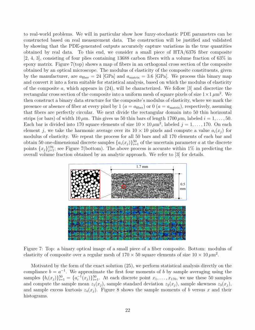
to real-world problems. We will in particular show how fuzzy-stochastic PDE parameters can beconstructed based on real measurement data. The construction will be justified and validatedby showing that the PDE-generated outputs accurately capture variations in the true quantitiesobtained by real data. To this end, we consider a small piece of HTA/6376 fiber composite[2, 4, 3], consisting of four plies containing 13688 carbon fibers with a volume fraction of 63% inepoxy matrix. Figure 7(top) shows a map of fibers in an orthogonal cross section of the compositeobtained by an optical microscope. The modulus of elasticity of the composite constituents, givenby the manufacturer, are afiber = 24 [GPa] and amatrix = 3.6 [GPa]. We process this binary mapand convert it into a form suitable for statistical analysis, based on which the modulus of elasticityof the composite a, which appears in (24), will be characterized. We follow [3] and discretize therectangular cross section of the composite into a uniform mesh of square pixels of size 1×1µm2. Wethen construct a binary data structure for the composite’s modulus of elasticity, where we mark thepresence or absence of fiber at every pixel by 1 (a = afiber) or 0 (a = amatrix), respectively, assumingthat fibers are perfectly circular. We next divide the rectangular domain into 50 thin horizontalstrips (or bars) of width 10µm. This gives us 50 thin bars of length 1700µm, labeled i = 1, . . . , 50.Each bar is divided into 170 square elements of size 10× 10µm2, labeled j = 1, . . . , 170. On eachelement j, we take the harmonic average over its 10 × 10 pixels and compute a value ai(xj) formodulus of elasticity. We repeat the process for all 50 bars and all 170 elements of each bar andobtain 50 one-dimensional discrete samples ai(xj)50
i=1 of the uncertain parameter a at the discretepoints xj170
j=1; see Figure 7(bottom). The above process is accurate within 1% in predicting theoverall volume fraction obtained by an analytic approach. We refer to [3] for details.
I. BabuSka et ul. I Comput. Methods A@. Mech. Engrg. I72 (1999) 27-77 29
Table 1 Material constants of the composite under consideration
E ,,her = 24 GPa qlhcr = 0.24 Gm = E,,,,r’X + ~,t,cr) E rnatr,x = 3.6 GPa Twr,x = 0.3 G mltrlx = Ernmx ‘Xl + Gt,,,)
Fig. 2. The group of four unidirectional plies. Note the of the matrix-rich zones between the plies.
visibility Fig. 3. Part of the complete large-size micrograph (a) Gray level image; (b) binary image.
So far, we have considered only one cross-section. Although in our analysis we will assume that the fibers are perfectly aligned, in reality they exhibit misalignment about their average direction. This microstructural characteristic is often referred as fiber undulation or fiber waviness. To get information about the waviness, 15 parallel cuts of the material were made, 50 pm apart with a precision of 2 km, and the positions of the fibers in these crossections were obtained by the technique described above.
In Fig. 4 we show the centers of the fibers in the 15 sections in a window of 2000 fibers. The figure clearly shows clearly the waviness of the fibers. We see that in the matrix regions between plies (compare Fig. 2) the fiber undulations are large, most likely due to small numbers of neighboring fibers. The maximum angle between any fiber and the z-axis is 6” with the standard deviation 1.2”.
The distribution of the fibers in the cross section was determinated by optical microscope. The size of the observation window was approximately 400 X 400 pm.
The cross-section samples were carefully polished with several series of different sized diamond particles in standard equipment for metallographic specimen preparation. The final polishing was performed with a 1 pm diamond spray on a hard cloth in order to obtain the best possible edge sharpness between the two phases in digital images.
The microstructure was digitized into an &bit digital image, i.e. a grey level image, by a CCD-camera located on a optical microscope. The images were then further processed by image processing and analysis software.
After the image acquisition, some initial pre-processing of the raw image was performed, such as contrast enhancement and filtering. In this way the images become standardized, which facilitated the extraction of the size and location of each fiber from the image. Magnification was chosen so that one pixel in the acquired image corresponded to an actual physical square with side 0.26 km.
The procedure after the image pre-processing involved separation of the fibers from the background of the matrix (image segmentation) and computing the location and.size of the fibers. In the microscope the fibers appear as objects of high brightness surrounded by a background with lower intensity corresponding to the matrix phase. The grey level distribution of the digitized image contained two peaks, corresponding to the matrix and the carbon fibers. The separation of the fibers from the background was performed by threshholding the grey level images. This operation allowed the fibers to be extracted from the matrix background. To assure reproducibility, the grey level threshold was chosen as the average of the gray levels at the two peaks. From the threshholding, a binary image was constructed in which the fiber and the matrix had different assigned values. However, in order to take into account the variation of the grey level distribution over the complete image, the threshholding was performed in a localized manner. Each image was divided into subimages, of approximate size 500 pixels by 500 pixels, where the threshhold levels were separately determined.
1.7 mm
0.5mm
2
4 5 6 7 8 9 100
500
1000
1500
2000
# fib
ers
fiber’s diameter [ ]
2 Problem Statement
Reliable mathematical and computational models for predicting the response of fiber compos-ites due to external forces must be designed based on and backed by real experimental data.In this section, we first present the real data that is used throughout this work. We thenconsider the deformation of fiber composites and describe the mathematical formulation of asimplified one-dimensional problem. Finally, we briefly address different models for treatinguncertainty in the problem.
2.1 Real data
The real data that we use are obtained from a small piece of a HTA/6376 carbon fiber-reinforced epoxy composite plate [11, 15] with a rectangular cross section of size 1.7×0.5 mm2,and consisting of four plies containing 13688 unidirectional fibers with a volume fraction of63%. Fiber diameters vary between 4µm to 10µm. Figure 2 shows a map of the size andposition of fibers in an orthogonal cross section of the composite obtained by an optical mi-croscope. In the present work, this particular map serves as a prototype of fiber distributionsin fiber composites.
Figure 2: Left: A 1.7 × 0.5 mm2 rectangular orthogonal cross section of a small piece of afiber composite laminate consisting of four uni-directional plies containing 13688 fibers witha volume fraction of 63%. Right: A binary image of a small part of the whole micrograph.
The Young’s modulus of elasticity and Poisson’s ratio of the fiber composite under con-sideration are given in Table 1.
Table 1: Material constants for the composite under consideration.
composite phases a ν
fiber 24 [GPa] 0.24matrix 3.6 [GPa] 0.3
2.2 Mathematical formulation: a one-dimensional problem
The deformation of elastic materials is given by the elastic partial differential equations(PDEs) in three dimensions. In the particular case of plane strain, where the length of
5
Figure 7: Top: a binary optical image of a small piece of a fiber composite. Bottom: modulus ofelasticity of composite over a regular mesh of 170× 50 square elements of size 10× 10µm2.
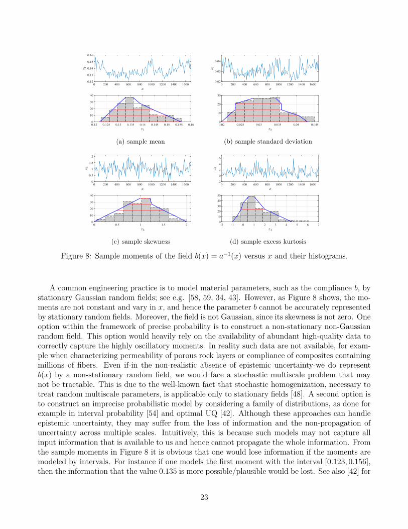
Motivated by the form of the exact solution (25), we perform statistical analysis directly on thecompliance b = a−1. We approximate the first four moments of b by sample averaging using thesamples bi(xj)50
i=1 = a−1i (xj)50
i=1. At each discrete point x1, . . . , x170, we use these 50 samplesand compute the sample mean z1(xj), sample standard deviation z2(xj), sample skewness z3(xj),and sample excess kurtosis z4(xj). Figure 8 shows the sample moments of b versus x and theirhistograms.
22
x
0 200 400 600 800 1000 1200 1400 1600z1
0.12
0.13
0.14
0.15
0.16
z1
0.12 0.125 0.13 0.135 0.14 0.145 0.15 0.155 0.160
10
20
30
40
(a) sample mean
x
0 200 400 600 800 1000 1200 1400 1600
z2
0.02
0.03
0.04
z2
0.02 0.025 0.03 0.035 0.04 0.0450
10
20
30
(b) sample standard deviation
x
0 200 400 600 800 1000 1200 1400 1600
z3
0
0.5
1
1.5
2
z3
0 0.5 1 1.5 20
10
20
30
40
(c) sample skewness
x
0 200 400 600 800 1000 1200 1400 1600
z4
-2
0
2
4
6
z4
-2 -1 0 1 2 3 4 5 6 70
10
20
30
40
50
(d) sample excess kurtosis
Figure 8: Sample moments of the field b(x) = a−1(x) versus x and their histograms.
A common engineering practice is to model material parameters, such as the compliance b, bystationary Gaussian random fields; see e.g. [58, 59, 34, 43]. However, as Figure 8 shows, the mo-ments are not constant and vary in x, and hence the parameter b cannot be accurately representedby stationary random fields. Moreover, the field is not Gaussian, since its skewness is not zero. Oneoption within the framework of precise probability is to construct a non-stationary non-Gaussianrandom field. This option would heavily rely on the availability of abundant high-quality data tocorrectly capture the highly oscillatory moments. In reality such data are not available, for exam-ple when characterizing permeability of porous rock layers or compliance of composites containingmillions of fibers. Even if-in the non-realistic absence of epistemic uncertainty-we do representb(x) by a non-stationary random field, we would face a stochastic multiscale problem that maynot be tractable. This is due to the well-known fact that stochastic homogenization, necessary totreat random multiscale parameters, is applicable only to stationary fields [48]. A second option isto construct an imprecise probabilistic model by considering a family of distributions, as done forexample in interval probability [54] and optimal UQ [42]. Although these approaches can handleepistemic uncertainty, they may suffer from the loss of information and the non-propagation ofuncertainty across multiple scales. Intuitively, this is because such models may not capture allinput information that is available to us and hence cannot propagate the whole information. Fromthe sample moments in Figure 8 it is obvious that one would lose information if the moments aremodeled by intervals. For instance if one models the first moment with the interval [0.123, 0.156],then the information that the value 0.135 is more possible/plausible would be lost. See also [42] for
23

an illustrative example of the non-propagation of ucertainty accross multiple scales. Among theimprecise probabilistic models, second-order hierarchical models [23] may be capable of treatingthis multiscale problem. In this case one may be able to model b by a random field with randommoments. Here, we propose another alternative beyond the framework of probability. In order toaccurately model and propagate uncertainty and afford multiscale strategies, we propose to modelthe parameter b by a fuzzy-stationary random field as follows.
We first fuzzify the moments of b: we use the histograms of the sample moments to constructmembership functions µz1 , µz2 , µz3 , µz4 . This can be done, for instance, by the method of leastsquares and with piecewise-linear regression functions (the thick blue lines in Figure 8). We thennormalize the regression functions so that the maximum membership function value is one. It isto be noted that this procedure generates an initial draft for membership functions. We may needto conduct a subsequent modification and make additional corrections, for instance if the initialdraft is not quasi-concave. Here, we use five α-levels (0, 0.25, 0.5, 0.75, 1) for the construction andobtain four decagonal fuzzy variables, described by their ten vertices
z1 = 〈0.1222, 0.1249, 0.1277, 0.1304, 0.1330, 0.1360, 0.1388, 0.1445, 0.1502, 0.1559〉,z2 = 〈0.0200, 0.0217, 0.0236, 0.0236, 0.0285, 0.0345, 0.0360, 0.0360, 0.0408, 0.0430〉,z3 = 〈0, 0.25, 0.50, 0.75, 1.00, 1.20, 1.25, 1.50, 1.75, 2.00〉,z4 = 〈−1.00, −0.55, −0.20, 0, 0.50, 1.00, 1.50, 2.00, 3.30, 4.50〉.
We note that the four fuzzy variables are fully interactive, because the four moments areobtained from the same set of data bi(xj)50
i=1 and hence are directly related to each other, that is,higher moments are obtained from lower moments. This will result in a reduction in fuzzy spacedimension. While we have a vector of four fuzzy variables z = (z1, z2, z3, z4), their joint α-cut S z
α
is a piecewise linear one-dimensional curve embedded in R4. Similar to the numerical example 1and using the arc length parameterization of the curve, we can represent S z
α by a piecewise linearmap.
We then construct a fuzzy-stochastic translation field to model the compliance:
b(x,y, z) = Ψ−1(z) Φ(G(x,y)). (28)
Here, Ψ(z) is the CDF of a four-parameter beta distribution determined by the four fuzzy moments,Φ is the standard normal CDF, and G(x,y) is a standard Gaussian field, approximated by thetruncated KL expansion: G(x,y) ≈ ∑m
j=1
√λj φj(x) yj, with yj ∼ N (0, 1) and the eigenpairs
(λj, φj(x))mj=1 of the deterministic covariance
C(x1, x2) = exp(−|x1 − x2|p
2 `2
), p = 2, ` = 20µm. (29)
We note that the selection of the covariance function and its parameters, such as the exponentp and correlation length `, must be based on a systematic calibration-validation strategy; see[6, 3]. As we will see in Figure 9, the choice (29) here delivers output quantities which fit the truequantities. Here, we choose m = 27 KL terms to preserve 90% of the unit variance of the Gaussianfield G.
The construction (28) has several advantages. First, it benefits from the simplicity of workingwith a stationary Gaussian field G(x,y). Moreover, by applying the inverse of Ψ on Φ(G) ∈
24

[0, 1], we obtain a field that achieves the target marginal fuzzy CDF Ψ(z). Finally, since thefuzzy moments are x-independent, the field (28) may be thought of as a fuzzy-stationary randomfield. One can hence employ global-local homogenization methods [3] and perform multiscalecomputations if needed.
We now let L = 1.7×10⁻³m and consider the problem (24) with the fuzzy-stochastic parametera = b−1 given by (28). Hence, the analytical solution (25) reads u(x,y, z) =
∫ x0 b(ξ,y, z) dξ.
We consider the following QoIs
Q4(x) = Q4(x, z) = E[u(x,y, z)],Q5(y) = Q5(y, z) = u(L/4, y, z),Q6 = Q6(z) = P (u(L/4,y, z) ≥ ucr).
Here, Q4 is a fuzzy field, Q5 is a fuzzy-stochastic function, and Q6 is a fuzzy failure probability.We now discuss the computation of the above three quantities.
The computation of Q4 and Q5 is similar to that of Q2 and Q3 in Section 5.1. Figure 9 showsthe fuzzy field Q4(x) versus x ∈ [0, 1000]µm (left) and the fuzzy CDF of Q5 for three membershipdegrees α = 0, 0.5, 1. We also compute and plot the “true” quantities directly obtained by thereal data, i.e. the 50 discrete samples, as follows. First, we choose Nb = 20 groups of samples,where each group consists of Mb = 15 different, randomly selected samples out of 50 discretesamples. For each group we then compute Mb samples of the true quantity and then obtain theirexpected value (to compare with Q4) and their CDF (to compare with Q5). This gives us a set ofNb benchmark solutions, referred to as the “truth". It is to be noted that the variations in truequantities reflect the presence of non-random uncertainty and justify the need for models beyondprecise probability. For instance for Q5 we obtain a range of distributions, hence forming a nestedset of p-boxes, instead of one single distribution that one may obtain in the absence of non-randomuncertainty. Figure 9 shows how accurately the computed quantities obtained by the proposedfuzzy-stochastic PDE model capture the variations in the true quantities.
x0 200 400 600 800 1000
Q4(x)
×10-4
0
0.5
1
1.5
2
exactα = 0α = 0.5α = 1
Q5 ×10-5
4 5 6 7 8 9
F(Q
5)
0
0.2
0.4
0.6
0.8
1
exactα = 0α = 0.25α = 0.50α = 0.75α = 1
Figure 9: The fuzzy field Q4(x) versus x (left) and the fuzzy CDF of Q5 (right). For comparison,the true quantities (thin turquoise curves) are included.
The quantity Q6 is the fuzzy probability of failure that would occur when the displacement uat x = L/4 reaches a critical value ucr. At every fixed α-level, we first uniformly discretize theone-dimensional joint α-cut S z
α into Mf discrete points z(k)Mf
k=1 ∈ S zα. We next set g(y, z) :=
ucr − u(L/4,y, z) and follow Algorithm 2 with q(y, z) = I[g(y,z)≤0]. We use Monte Carlo samplingwith Ms realizations y(i)Ms
i=1 to approximate
25

Q6(z(k)) = E[I[g(y,z(k))≤0]] ≈1Ms
Ms∑i=1
I[g(y(i),z(k))≤0], k = 1, . . . ,Mf . (30)
The output α-cut for Q6 is then obtained by
SQ6α =
[minkQ6(z(k)), max
kQ6(z(k))
]. (31)
Figure 10 shows the membership function of Q6 obtained from the α-cuts given in (30)-(31) com-puted for five α levels α = 0, 0.25, 0.5, 0.75, 1, with ucr = 6.9× 10⁻⁵ µm, Mf = 181, and Ms = 104.
Q6
0 0.05 0.1 0.15 0.2 0.25
µQ
6(Q
6)
0
0.2
0.4
0.6
0.8
1
1.2
Figure 10: The membership function of the fuzzy failure probability Q6 and its five α-cuts.
Note that the additional nuanced information given through nested intervals at different levelsof possibility of Q6 is a direct result of the propagation of additional nuanced information availablein the statistical moments in Figure 8. Such additional information may not be accounted forand hence would not be propagated though other imprecise probabilistic models, such as intervalprobabilities and optimal UQ. This is particularly important in “certification problems", where weneed to certify or decertify a system of interest. To illustrate this, let εTOL = 0.1 be the greatestacceptable failure probability Q6, that is, the system is safe if Q6 ≤ εTOL and unsafe if Q6 > εTOL.Suppose that the lower and upper bounds of the zero-cut of Q6, i.e. 0 and 0.2284, represents thecrisp lower and upper bounds obtained by an imprecise probabilistic approach. In this case since0 < εTOL = 0.1 < 0.224, then we cannot decide on the safety of the system, unless additionalinformation will be provided. However, the additional nuanced information provided by the lowerand upper bounds at different levels of possibility (i.e. different α-levels) may help decision-makers.In fact the highest level of possibility (the most possible scenario) corresponding to the 1-cut inFigure 10 suggests that the system may be safe.
5.3 Computational cost
Consider a fuzzy-stochastic function q(y, z), for example obtained by applying a combinationof algebraic, integral, and differential operators on the solution u(x,y, z) to a fuzzy-stochasticPDE problem. Assume that we are interested in computing a fuzzy quantity Q = E[q(y, z)]. Thecomputation of one α-cut SQα requiresMf function evaluationsQ(z(k)) = E[q(y, z(k))] atMf discretepoints z(k)Mf
k=1 ∈ S zα. At each discrete point the expectation of q needs to be approximated by a
sampling technique using Ms samples. In total we need to solve M = Mf Ms deterministic PDEproblems. The size of M depends mainly on the number of random variables m, the number of
26

fuzzy variables n, and the regularity of q with respect to y and z. When M is very large, e.g. inthe absence of high regularity or when m and n are large, the computations may be prohibitivelyexpensive. There are however practical situations where fuzzy-stochastic computations are feasible:
1. In many applications we have a low-dimensional fuzzy space, i.e. n m. A typical example iswhen we model an uncertain parameter, such as the compliance, by a hybrid fuzzy-stochasticfield. In this case, n is usually 1 (if the moments are fully interactive) or 2-4 (if we use 2-4non-interactive moments), while m may be rather large depending on the correlation lengthof the field. As a result, fuzzy-stochastic computations are usually not much more expensivecompared to solving purely stochastic problems.
2. When q is highly regular with respect to (y, z) we can employ spectral methods on sparsegrids instead of Monte Carlo sampling strategies in order to speed up the computations.The stochastic and fuzzy spaces are different considering we extract statistical informationin the stochastic space and perform optimization in the fuzzy space. Therefore, thanks tohigh reqularity, we may build a surrogate model of q(y, z) on the tensor product of twoseparate sparse grids (one on each space) using sparse interpolating polynomials; see e.g.[38, 39]. This type of separation affords efficient extraction of statistical information andsparse optimization [28, 31].
3. Current probabilistic models are usually not applicable to multiscale problems with highlyoscillatory uncertain parameters. It is well known that stochastic homogenization, necessaryto treat multiscale stochastic parameters, is applicable only to stationary random fields [48],while in many multiscale problems the moments are not constant. Another related problemwith imprecise probabilistic models is the non-propagation of uncertainty across multiplescales [42]. In such cases, a hybrid fuzzy-stochastic model may be considered as a feasibleand accurate approach to treat the problem; see [3] where a fuzzy-stochastic multiscaleapproach is presented for fiber composite polymers.
4. Due to the non-intrusiveness of the numerical methods, the M deterministic problems canbe distributed and solved independently on parallel computers.
We are currently working on the development of efficient numerical methods for solving fuzzy-stochastic PDE problems. We are also exploring more applications involving time-dependent PDEsto be presented elsewhere.
Acknowledgments
I am indebted to Ivo Babuška for introducing me to the field of fuzzy calculus and for our regular,long stimulating discussions on uncertainty quantification and fuzzy-stochastic modeling.
References
[1] American Society for Metals. Thermal properties of metals. In F. Cverna, editor, ASM ReadyReference, ASM Materials Data Series. ASM International, Materials Park, Ohio, 2002.
27
[2] I. Babuška, B. Andersson, P. J. Smith, and K. Levin. Damage analysis of fiber composites,Part I: statistical analysis on fiber scale. Comput. Methods Appl. Mech. Engrg., 172:27–77,1999.
[3] I. Babuška and M. Motamed. A fuzzy-stochastic multiscale model for fiber composites: A one-dimensional study. Computer Methods in Applied Mechanics and Engineering, 302:109–130,2016.
[4] I. Babuška, M. Motamed, and R. Tempone. A stochastic multiscale method for the elastody-namic wave equations arising from fiber composites. Computer Methods in Applied Mechanicsand Engineering, 276:190–211, 2014.
[5] I. Babuška, F. Nobile, and R. Tempone. A stochastic collocation method for elliptic partialdifferential equations with random input data. SIAM J. Numer. Anal., 45:1005–1034, 2007.
[6] I. Babuška, F. Nobile, and R. Tempone. A systematic approach to model validation basedon Bayesian updates and prediction related rejection criteria. Comput. Methods Appl. Mech.Engrg., 197:2517–2539, 2008.
[7] I. Babuška and J. T. Oden. Verification and validation in computational engineering andscience: Part I, basic concepts. Computer Methods in Applied Mechanics and Engineering,193:4047–4068, 2004.
[8] I. Babuška and R. S. Silva. Numerical treatment of engineering problems with uncertainties:the fuzzy set approach and its application to the heat exchange problem. Int. J. Numer.Meth. Engng., 87:115–148, 2011.
[9] I. Babuška, R. Tempone, and G. E. Zouraris. Solving elliptic boundary value problems withuncertain coefficients by the finite element method: the stochastic formulation. ComputerMethods in Applied Mechanics and Engineering, 194:1251–1294, 2005.
[10] A. M. Bertone, R. M. Jafelice, L. C. de Barros, and R. C. Bassanezi. On fuzzy solutions forpartial differential equations. Fuzzy Sets and Systems, 219:68–80, 2013.
[11] J. J. Buckley. Fuzzy Probability and Statistics. Springer, Berlin, 2006.
[12] J. J. Buckley and T. Feuring. Introduction to fuzzy partial differential equations. Fuzzy Setsand Systems, 105:241–248, 1999.
[13] C. Carlsson, R. Fullér, and P. Majlender. Additions of completely correlated fuzzy numbers.In Proceedings of IEEE International Conference on Fuzzy Systems, pages 535–539, Budapest,2004.
[14] A. Chernatynskiy, S. R. Phillpot, and R. LeSar. Uncertainty quantification in multiscalesimulation of materials: A prospective. Annual Review of Materials Research, 43:157–182,2013.
28

[15] K. A. Cliffe, M. B. Giles, R. Scheichl, and A. L. Teckentrup. Multilevel Monte Carlo methodsand applications to elliptic PDEs with random coefficients. Comput. Visual Sci., 14:3–15,2011.
[16] S. Corveleyn, E. Rosseel, and S. Vandewalle. Iterative solvers for a spectral Galerkin approachto elliptic partial differential equations with fuzzy coefficients. SIAM J. Sci. Comput., 35:S420–S444, 2013.
[17] I. Couso, D. Dubois, and L. Sanchez. Random Sets and Random Fuzzy Sets as Ill-PerceivedRandom Variables. Springer, New York, 2014.
[18] D. Dubois and H. Prade. Fuzzy Sets and Systems-Theory and Applications. Academic Press,Inc., San Diego, 1980.
[19] D. Dubois and H. Prade. Formal representations of uncertainty. In D. Bouyssou, D. Dubois,H. Prade, and M. Pirlot, editors, Decision Making Process: Concepts and Methods, pages85–157. Wiley-ISTE, 2010.
[20] L. C. Evans. Partial Differential Equations, volume 19 of Graduate Studies in Mathematics.American Mathematical Society, Providence, Rhode Island, 1998.
[21] G. S. Fishman. Monte Carlo: Concepts, Algorithms, and Applications. Springer- Verlag, NewYork, 1996.
[22] R. Fullér. On generalization of Nguyen’s theorem: A short survey of recent developments. InJ. Fodor and R. Fullér, editors, Advances in soft computing, intelligent robotics and control,volume 8 of Topics in Intelligent Engineering and Informatics, pages 183–190. Springer, 2014.
[23] A. Gelman, J. B. Carlin, H. S. Stern, and D. B. Rubin. Bayesian data analysis. Chapmanand Hall/CRC, 2004.
[24] R. G. Ghanem and P. D. Spanos. Stochastic finite elements: A spectral approach. Springer,New York, 1991.
[25] M. Grigoriu. Stochastic Calculus, Applications in Sciences and Engineering. Birkhäuser,Boston, 2002.
[26] A.-L. Haji-Ali, F. Nobile, and R. Tempone. Multi-index Monte Carlo: when sparsity meetssampling. Numerische Mathematik, 132:767–806, 2016.
[27] T. Y. Hou and X. Wu. Quasi-Monte Carlo methods for elliptic PDEs with random coefficientsand applications. J. Comput. Phys., 230:3668–3694, 2011.
[28] L. Jaulin, M. Kieffer, O. Didrit, and E. Walter. Applied Interval Analysis, with Examplesin Parameter and State Estimation, Robust Control and Robotics. Springer-Verlag, London,2001.
[29] J. Kaipo and E. Somersalo. Statistical and Computational Inverse Problems. Springer, NewYork, 2005.
29

[30] G. J. Klir. Uncertainty and Information: Foundations of Generalized Information Theory.Wiley, New Jersey, 2005.
[31] T. G. Kolda, R. M. Lewis, and V. Torczon. Optimization by direct search: new perspectiveson classical and modern methods. SIAM Review, 45:385–482, 2003.
[32] H. Kwakernaak. Fuzzy random variables - I. Definitions and theorems. Information Sciences,15:1–29, 1978.
[33] H. Kwakernaak. Fuzzy random variables - II. Algorithems and examples for the discrete case.Information Sciences, 17:253–278, 1979.
[34] W. K. Liu, D. Qian, S. Gonella, S. Li, W. Chen, and S. Chirputkar. Multiscale methods formechanical science of complex materials: Bridging from quantum to stochastic multiresolutioncontinuum. International Journal for Numerical Methods in Engineering, 83:1039–1080, 2010.
[35] B. Möller and M. Beer. Fuzzy Randomness. Springer, New York, 2004.
[36] R. E. Moore, R. B. Kearfott, and M. J. Cloud. Introduction to Interval Analysis. SIAM Press,Philadelphia, Pennsylvania, 2009.
[37] M. Motamed and D. Appelö. A multi-order discontinuous Galerkin Monte Carlo method forhyperbolic problems with stochastic parameters. Submitted to SIAM J. Numer. Anal., 2016.
[38] M. Motamed, F. Nobile, and R. Tempone. A stochastic collocation method for the secondorder wave equation with a discontinuous random speed. Numer. Math., 123:493–536, 2013.
[39] M. Motamed, F. Nobile, and R. Tempone. Analysis and computation of the elastic waveequation with random coefficients. Computers and Mathematics with Applications, 70:2454–2473, 2015.
[40] A. Neumaier. Complete search in continuous global optimization and constraint satisfaction.Acta Numerica, 13:15–83, 2004.
[41] H. T. Nguyen. A note on the extension principle for fuzzy sets. Journal of MathematicalAnalysis and Applications, 64:369–380, 1978.
[42] H. Owhadi, C. Scovel, T. J. Sullivan, M. McKerns, and M. Ortiz. Optimal uncertaintyquantification. SIAM Review, 55:271–345, 2013.
[43] M. Papadrakakis and G. Stefanou (Eds.). Multiscale Modeling and Uncertainty Quantificationof Materials and Structures. Springer, Cambridge, 2014.
[44] T. J. Ross. Fuzzy Logic with Engineering Applications. Wiley, Singapore, 2010.
[45] K. Scheerlinck, H. Vernieuwe, and B. De Baets. Zadeh’s extension principle for continuousfunctions of non-interactive variables: A parallel optimization approach. IEEE Transactionson Fuzzy Systems, 20:96–108, 2012.
30

[46] K. Scheerlinck, H. Vernieuwe, N.E.C. Verhoest, and B. De Baets. Practical computing withinteractive fuzzy variables. Applied Soft Computing, 22:518–527, 2014.
[47] G. Shafer. A Mathematical Theory of Evidence. Princeton University Press, NJ, 1976.
[48] P. E. Souganidis. Stochastic homogenization of Hamilton-Jacobi equations and some applica-tions. Asymptotic Analysis, 20:1–11, 1999.
[49] A. M. Stuart. Inverse problems: A Bayesian perspective. Acta Numerica, 19:451–559, 2010.
[50] T. J. Sullivan. Introduction to Uncertainty Quantification. Springer, 2015.
[51] Y. S. Touloukian, R. W. Powell, C. Y. Ho, and P. G. Klemens. Thermal conductivity - metallicelements and alloys. In Thermophysical Properties of Matter, volume 1 of The TPRC DataSeries. 1970.
[52] P. Walley. Statistical Reasoning with Imprecise Probabilities. Chapman and Hall, London,1991.
[53] P. Walley. Towards a unified theory of imprecise probability. International Journal of Ap-proximate Reasoning, 24:125–148, 2000.
[54] K. Weichselberger. The theory of interval probability as a unifying concept for uncertainty.International Journal of Approximate Reasoning, 24:149–170, 2000.
[55] D. Xiu. Numerical Methods For Stochastic Computations: A spectral method approach. Prince-ton University Press, 2010.
[56] D. Xiu and J. S. Hesthaven. High-order collocation methods for differential equations withrandom inputs. SIAM J. Sci. Comput., 27:1118–1139, 2005.
[57] D. Xiu and G. E. Karniadakis. Modeling uncertainty in steady state diffusion problems viageneralized polynomial chaos. Computer Methods in Applied Mechanics and Engineering,191:4927–4948, 2002.
[58] X. F. Xu and L. Graham-Brady. A stochastic computational method for evaluation of globaland local behavior of random elastic media. Computer Methods in Applied Mechanics andEngineering, 194:4362–4385, 2005.
[59] X. Yin, S. Lee, W. Chen, and W. K. Liu. Efficient random field uncertainty propagationin design using multiscale analysis. Journal of Mechanical Design, 131:021006–1–021006–10,2009.
[60] L. A. Zadeh. Fuzzy sets. Information and Control, 8:338–353, 1965.
[61] L. A. Zadeh. The concept of a linguistic variable and its application to approximate reasoning.Information Sciences, 8:199–249, 1975.
[62] L. A. Zadeh. Fuzzy probabilities. Informarion Processing and Management, 20:363–372, 1984.
31