ýg joint program in oceanography/ 4 applied ocean … reflection and tunneling of ocean waves ......

MIT/WHOI 2006-17

Massachusetts Institute of Technology

Woods Hole Oceanographic Institution

ýG joint Program 4

in Oceanography/ 4oFhC Applied Ocean Science 1930

and Engineering

DOCTORAL DISSERTATION

Infragravity Waves Over Topography:

Generation, Dissipation, and Reflection

by

James M. Thomson

September 2006

DISTRIBUTION STATEMENT AApproved for Public Release

oistribution Unlimited

MIT/WHOI

2006-17

Ilfragravity Waves Over Topography:Generation, Dissipation, and Reflection

by

James M. Thomson

Massachusetts Institute of TechnologyCambridge, Massachusetts 02139

and

Woods Hole Oceanographic InstitutionWoods Hole, Massachusetts 02543

September 2006

DOCTORAL DISSERTATION

Funding was provided by the Office of Naval Research (Coastal Geosciences Program,N00014-02-10145), the National Science Foundation (Physical Oceanography,

OCE-0115850), and the WHOI Academic Programs Office.

Reproduction in whole or in part is permitted for any purpose of the United StatesGovernment. This thesis should be cited as: James M. Thomson, 2006. Infragravity Waves

Over Topography: Generation, Dissipation, and Reflection. Ph.D. Thesis. MIT/WHOI,2006-17.

Approved for publication; distribution unlimited.

Approved for Distribution:

Robert A. Weller, Chair

Department of Physical Oceanography

Paola Malanotte-Rizzoli James A. YoderMIT Director of JointProgram WHOI Dean of Graduate Studies

Infragravity Waves over Topography:


by

James M. Thomson

Submitted to the Joint Program in Physical Oceanographyin partial fufillment of the requirements for the degree of

Doctor of Philosophy

at the

MASSACHUSETTS INSTITUTE OF TECHNOLOGY

and the

WOODS HOLE OCEANOGRAPHIC INSTITUTION

September 2006

©WHOI, 2006. All rights reserved.

Author ........ .......Joint Program in Physical Oceanography

August 16, 2006

Certified by.-, *% ......Steve Elgar

Senior Scientist, WHOIThesis Supervisor

Accepted by ...... .................""Joseph Pedlosky

Chairman, Joint Committee for Physical Oceanography

Infragravity Waves over Topography:


by

James M. Thomson

Submitted to the Joint Program in Physical Oceanographyon August 16, 2006, in partial fulfillment of the

requirements for the degree ofDoctor of Philosophy

Abstract

Ocean surface infragravity waves (periods from 20 to 200 s) observed along the south-ern California coast are shown to be sensitive to the bottom topography of the shelfregion, where propagation is linear, and of the nearshore region, where nonlinearityis important. Infragravity waves exchange energy with swell and wind waves (periodsfrom 5 to 20 s) via conservative nonlinear interactions that approach resonance withdecreasing water depth. Consistent with previous results, it is shown here that aswaves shoal into water less than a few meters deep, energy is transfered from swellto infragravity waves. In addition, it is shown here that the apparent dissipation ofinfragravity energy observed in the surfzone is the result of nonlinear energy trans-fers from infragravity waves back to swell and wind waves. The energy transfers aresensitive to the shallow water bottom topography. On nonplanar beach profiles thetransfers, and thus the amount of infragravity energy available for reflection from theshoreline, change with the tide, resulting in the tidal modulation of infragravity en-ergy observed in bottom-pressure records on the continental shelf. The observed wavepropagation over the shelf topography is dominated by refraction, and the observedpartial reflection from, and transmission across, a steep-walled submarine canyon isconsistent with long-wave theory. A generalized regional model incorporating theseresults predicts the observed infragravity wave amplitudes over variable bottom to-pography.

Thesis Supervisor: Steve ElgarTitle: Senior Scientist, WHOI

3

Acknowledgments

I thank the Office of Naval Research (Coastal Geosciences Program, N00014-02-

10145), the National Science Foundation (Physical Oceanography, OCE-0115850),

and the Academic Programs office at WHOI for their generous support.

My advisor, Dr. Steve Elgar, has contributed tirelessly to this work and to my

professional development. He has taught, challenged, and encouraged me in an ap-

prenticeship beyond my highest expectations.

Committee members and coauthors, Drs. David Chapman, Robert Guza, Thomas

Herbers, Steve Lentz, Joseph Pedlosky, Britt Raubenheimer, and Carl Wunsch, have

patiently advised, contributed, questioned, and listened. I am grateful for their col-

laborations and instruction.

The field observations were made possible by many dedicated professionals at

WHOI, the Scripps Institute of Oceanography, the Naval Postgraduate School, and

Ohio State University. Of the many contributions, Peter Schultz's efforts have been

paramount. I am proud of the work we have done together, and I am grateful for his

expertise, enthusiasm, and friendship.

I also thank Alex Apotsos, Melanie Fewings, Greg Gerbi, Carlos Moffat, Andrew

Mosedale, Dave Sutherland, and my other peers in the Joint Program who have

enhanced my experience and education greatly.

Many thanks go to my family as well, who always have encouraged me to work

hard and enjoy what I do.

And my gracious wife, Jess, I will be thanking for a long, long time. She has

fed hungry fieldcrews, braved the many uncertainties of these five years, encouraged

every small bit of progress, and provided a source of calmness and levity to each of

my days. Many new things are in our future together, and I look forward to all of

them.

5

Contents

1 Introduction 11

1.1 Thesis Outline ....................................... 12

1.2 Background ......... ................................ 12

1.3 The Nearshore Canyon Experiment ......................... 16

2 Tidal Modulation of Infragravity Waves via Nonlinear Energy Losses

in the Surfzone 23

2.1 Introduction ......... ................................ 24

2.2 Field Observations . . ... ....................... 26

2.3 Analysis .......... .................................. 28

2.3.1 Nonlinear Energy Balance ........................... 29

2.3.2 Numerical Model ........ ......................... 32

2.3.3 Bottom Profile Dependence ......................... 34

2.4 Conclusions ......... ................................ 34

3 Reflection and tunneling of ocean waves observed at a submarine

canyon 41

3.1 Introduction ......... ................................ 42

3.2 Theory ......... ................................... 42

3.3 Field Observations ........ ............................ 48

3.4 Methods .......... .................................. 49

7

3.5 Results ......... ................................... 52

3.6 Conclusions ......... ................................ 55

4 Conclusions and Regional Description 59

4.1 Shoaling and Unshoaling ................................ 59

4.2 Refraction and Canyon Reflections ...... ................... 60

4.2.1 Case Study ........ ............................ 64

4.2.2 Climatology ........ ............................ 66

4.2.3 Model Skill ........ ............................ 66

4.3 Suggested Applications .................................. 69

8

List of Figures

1-1 Infragravity schematic ........ .......................... 13

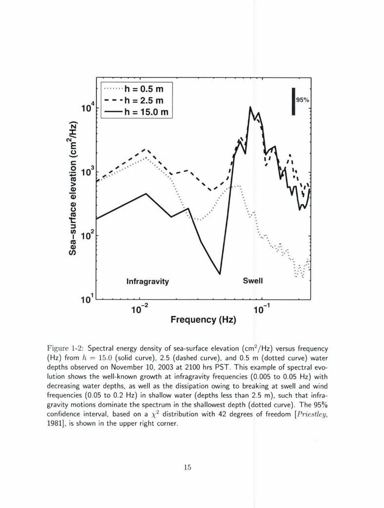
1-2 Example energy spectra ........ ......................... 15

1-3 Nearshore Canyon Experiment array and bathymetry ............. 17

1-4 Nearshore Canyon Experiment data summary ................. 19

2-1 Example of tidal modulation ............................. 25

2-2 Cross-shore energy flux profiles ....... ..................... 27

2-3 Nonlinear exchange in the surfzone ...... ................... 31

2-4 Cross-shore evolution of biphase ........................... 33

2-5 Bottom profile dependence at all transects .................... 35

3-1 Detailed bathynmetry at La Jolla canyon ...... ................ 43

3-2 Reflection coefficients versus frequency ...................... 45

3-3 Schematic of reflection and tunneling ...... .................. 47

3-4 Phase shift during reflection ....... ....................... 54

4-1 Infragravity shoaling dominated by free waves ................. 61

4-2 Example ray paths using refraction-reflection model .............. 63

4-3 Case study of infragravity variance along isobaths ............... 65

4-4 Average infragravity variance along isobaths ................... 67

4-5 Refraction model-data comparison .......................... 68

9

Chapter 1

Introduction

Infragravity waves are oscillatory motions of the ocean surface with periods of or-

der one minute. These waves are strongest near the shoreline [Guza and Thornton,

1985], where usually they are coupled to higher frequency surface motions (swell and

wind waves) [Elgar et al., 1992]. Most observations of infragravity waves have been

in regions with gently varying bottom topography [Herbers et al., 1995b]. Here, in-

fragravity waves propagating over rapidly varying topography are investigated using

field observations, analytic theories, and numerical models. The specific objectives

are to:

"* identify the sources and sinks of infragravity motions,

"* determine the cause of a tidal modulation of infragravity energy observed at

offshore locations, and

"* test a long-wave prediction for the reflection and transmission of infragravity

waves from a steep-walled submarine canyon.

The results are generalized to formulate a descriptive regional model. Although a

full scale modeling effort is beyond the scope of the thesis, the results identify the

processes that should be included to model infragravity waves accurately, and indicate

several possible improvements to existing models.

11

1.1 Thesis Outline

Background information on infragravity waves, a review of previous work, and general

information regarding the field data collection are presented in Chapter 1. Results

from detailed process studies are presented as independent articles (i.e., separate

abstracts and bibliographies) in Chapters 2 and 3.

Chapter 2, "Tidal Modulation of Infragravity Waves via Nonlinear Energy Losses

in the Surfzone," is an extension of Thomson et al. [2006], and demonstrates that

infragravity wave energy is transfered to swell and wind waves in the surfzone, in

contrast with the well-known transfer of energy to infragravity waves from swell and

wind waves via nonlinear interactions in deeper water. This energy loss is enhanced

over the low tide beach profile, resulting in the tidal modulation of infragravity energy

observed offshore.

Chapter 3, "Reflection and Tunneling of Ocean Waves Observed at a Submarine

Canyon," is an extension of Thomson et al. [2005], including a detailed methods

section published online only, and describes the observational validation of a long-

wave theory for the partial reflection and transmission of infragravity waves at a

steep-walled submarine canyon.

Chapter 4 summarizes the results and suggests a descriptive model for the regional

distribution of infragravity energy based on the results in the previous chapters.

1.2 Background

Infragravity waves (surface gravity waves with periods of 20 to 200 s) were first ob-

served as a "surf beat" modulation coincident with groups of narrow-banded swell

(periods of 10 to 20 s) and having the period and wavelength ("- 500 in) of the groups

(Figure 1-1) [Munk, 1949, Tucker, 1950]. Subsequent investigations have shown that

these waves are important to alongshore currents in the surfzone [Sasaki, 1976], sed-

iment transport near the shoreline [Bauer and Greenwood, 1990], oscillations in har-

12

- .Swell

E 80- lnfragravity

6040

40

~20• - 0•. 0 - ,, , -

=-20

m-40-60

0 500 1000 1500 2000Distance (m)

Figure 1-1: Sea-surface elevation versus distance showing a group modulation in swell(periods from 10 to 20 s) waves (solid curve) and the accompanying forced infragravity(period from 20 to 200 s) wave (dashed curve). Group modulations are caused by thebeating of neighboring frequencies, and the resulting infragravity wave is forced at thecorresponding difference, or beat, frequency. In deep water, the forced infragravity waveremains small (amplitudes of a few cm). In shallow water, the forcing is near-resonantand large (1 m) amplitude infragravity waves can occur.

bors [Okihiro et al., 1993], and fluctuations in seismic records [Dolenc et al., 2005].

In deep water, nonresonant nonlinear quadratic interactions between swell waves

produce forced infragravity motions [Hasselmann, 1962]. Using a slowly varying

(WKBJ) approach in finite depth, this forcing can be expressed as excess momentum

flux owing to the swell groups [Longuet-Higgins and Stewart, 1962], and is consistent

with observations [Elgar et al., 1992, Herbers et al., 1994]. As waves enter shallow wa-

ter, the quadratic nonlinear interactions approach resonance, and in water less than

a few meters deep significant energy can be transfered from wind waves to infragrav-

ity motions over a few hundred meters of propagation [Gallagher, 1971, Elgar and

13

Guza, 1985, Herbers et al., 1995b, Ruessink et al., 1998; and others]. Thus, energy

at infragravity periods usually is low in the deep ocean and increases as water depth

decreases, reaching amplitudes up to 1 m at the shoreline (Figure 1-2).

When the swell waves break and dissipate in the surfzone, the infragravity waves

are released and propagate towards the shoreline as free waves [Herbers et al., 1995a].

Recent analysis suggests that in the surfzone infragravity waves transfer some energy

back to higher frequencies [Thomson et al., 2006, Henderson et al., submitted, 2006],

before reflecting from the shoreline [Suhayda, 1974, Guza and Thornton, 1985, Nelson

and Gonsalves, 1990, Elgar et al., 1994, Sheremet et al., 2002]. Reflected infragravity

waves can be refractively trapped (i.e., edge waves) close to the shore in a topographic

wave guide [Eckart, 1951, Huntley et al., 1981, Oltman-Shay and Guza, 1987; and

others] or can propagate to deep water obeying the linear finite depth dispersion

relation

w2 = gk tanh kh, (1.1)

where w is the radian frequency, g is the gravitational acceleration, k is the wavenum-

ber, and h is the water depth [Mei, 1989, §1.4]. Infragravity energy levels observed

seaward of the turning point for edge waves are dominated by free waves (i.e., leaky

waves) and characterized by broad frequency-directional spectra [Elgar et al., 1992,

Herbers et al., 1995a].

Previous investigations of infragravity waves have focused on regions with along-

shore homogeneous bathymetry. Consequently, the possible affects of rapidly varying

topography on infragravity wave propagation were untested [Holman and Bowen,

1984] prior to the recent observation of infragravity reflection and transmission at a

submarine canyon [Thomson et al., 2005]. By incorporating the observed strong re-

flections into standard ray tracing techniques, and applying a conservative nonlinear

energy balance [Thomson et al., 2006], predictive models for infragravity waves can

be improved.

14

h =0.5 m104 - -- h = 2.5 rn 95

O•" - h=15.Om IN

E

o,1I

CI

10- 10-

Frq c (

CO) 2

110

Infragravity Swell

Frequency (Hz)

Figure 1-2: Spectral energy density of sea-surface elevation (cm 2/Hz) versus frequency(Hz) from h = 15.0 (solid curve), 2.5 (dashed curve), and 0.5 m (dotted curve) waterdepths observed on November 10, 2003 at 2100 hrs PST. This example of spectral evo-lution shows the well-known growth at infragravity frequencies (0.005 to 0.05 Hz) withdecreasing water depths, as well as the dissipation owing to breaking at swell and windfrequencies (0.05 to 0.2 Hz) in shallow water (depths less than 2.5 in), such that infra-gravity motions dominate the spectrum in the shallowest depth (dotted curve). The 95%confidence interval, based on a X2 distribution with 42 degrees of freedom [Priestley,1981], is shown in the upper right corner.

15

1.3 The Nearshore Canyon Experiment

Data used in this thesis were collected as part of the Nearshore Canyon Experiment

(NCEX) during the fall of 2003. Specific information regarding data and methods is

presented within Chapters 2, 3, and 4. This section presents additional information.

An array of bottom-mounted current meters and pressure gages was maintained

along the southern California coast from September to December, 2003 (Figure 1-3).

The NCEX array was designed to study waves and currents near and onshore of two

steep submarine canyons. Additional instruments were deployed to study nonlinear

wave evolution (Chapter 2) across the surfzone and nearshore region at the northern

end of the array (y = 2.7 km, Figure 1-3), and to study partial wave reflection

(Chapter 3) from La Jolla canyon (y • -1.0 km, Figure 1-3). The data include a

range of wave (Figure 1-4) and atmospheric (not shown) conditions.

Colocated pressure and velocity data were collected hourly at 2 Hz for 3072 s

(51 min), although for a three-week period some data were collected at 16 Hz and

then subsampled to 2 Hz during the analysis. Setra pressure gages without colocated

velocity measurements sampled continuously at 2 Hz throughout the experiment, in-

terrupted by one (or two for some instruments) turn-arounds. In depths greater than

3 m, the colocated current meters (SonTek and NorTek acoustic Doppler velocimne-

ters) and pressure gages (ParoScientific and Druk resonant pressure transducers) were

mounted on fixed platforms within 1 m of the seafloor. In depths less than 3 m, the

pressure gages were buried up to 1 m to prevent flow noise [Raubenheimer et al., 1998].

After initial quality control to remove bad data, power spectra of pressure and each

of the three velocity components were calculated by subdividing the 3072 s records

into 1024 s windows with 75% overlap between adjacent windows, Fourier transform-

ing the data, and merging every seven neighboring frequency bands. The resulting

spectral values have 42 degrees of freedom [Priestley, 1981], and are corrected for

attenuation by the water column using linear finite depth theory (i.e., attenuation is

assumed to be proportional to cosh(kh) [Mei, 1989, §1.4]). In a test with two inde-

16

2.5

2.0

1.5

1.0

"0.5

0.0

-0.5

-1.0

-1.5

-2.0 -1.5 -1.0 -0.5 0.0x (km)

Figure 1-3: Nearshore Canyon Experiment instrument array (symbols) and bathymetry(shaded surface) using a local coordinate system (origin at the foot of the Scripps pier:32.8660 N, -117.2560 W) along the southern California coast (tan region). Bottommounted instruments measured pressure (open symbols), and pressure colocated withvelocity (filled symbols) for two months during the fall of 2003. Water depths range fromover 100 m (dark regions) in the Scripps (northern) and La Jolla (southern) canyons to0 m at the shoreline (boundary between the light blue shading and tan region).

17

pendent instruments deployed at the same location, the cross-spectra of pressure and

velocity from the two instruments were coherent above the 99.9% confidence level in

the frequency bands of interest (0.005 to 0.25 Hz).

Offshore bathymetry (Figure 1-3) was surveyed using shipboard acoustic equip-

ment prior to the experiment. Nearshore bathymetry was surveyed both prior to,

and weekly during, the experiment using a customized personal watercraft equip)ped

with a Differential Global Positioning System (DGPS), gryoscope, and sonar trans-

ducer. In addition, the acoustic current meters in less than 3 in depth estimated

the distance to the slowly changing seafloor every hour. The offshore bathymetry has

vertical errors of ±10 cm and horizontal errors of ±50 cm. The nearshore bathynietry

has vertical errors of ±10 cm and horizontal errors of ±5 cm. Changes in nearshore

bathymetry observed during the experiment were not sufficient to alter the results

of the nearshore study (Chapter 2), and thus a single survey from October was used

throughout the analysis.

18

(a) Nearshore infragravity variance100

E

50

(b) Offshore swell vaveprianc

1000-

CM

E500

2 1 1 1 1 1 1 1 1 1 1 1 1 .I I I I I I . . . . . . . . .

(c) Offshore mean wave period

1501

10 Wt

7 8 9 10111213141516171192021222324252627282930311 2 3 4 5 6 7 8 9 101112131415161716192021

October November

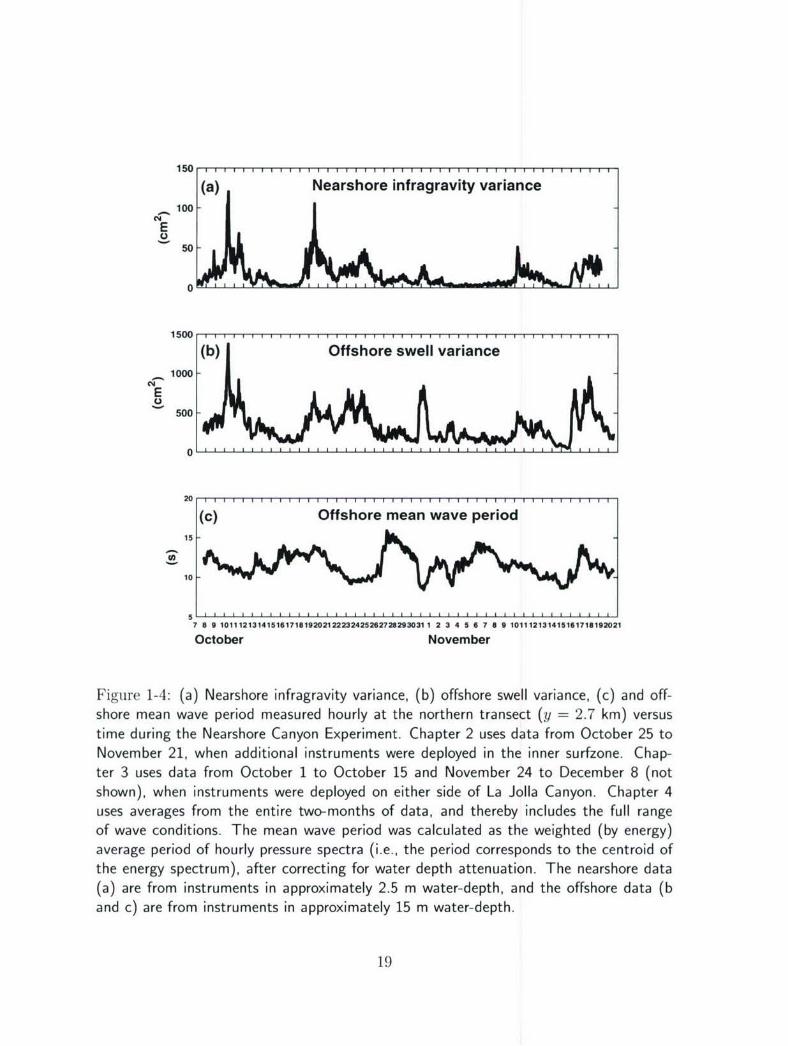
Figure 1-4: (a) Nearshore infragravity variance, (b) offshore swell variance, (c) and off-shore mean wave period measured hourly at the northern transect (y = 2.7 kin) versustime during the Nearshore Canyon Experiment. Chapter 2 uses data from October 25 toNovember 21, when additional instruments were deployed in the inner surfzone. Chap-ter 3 uses data from October 1 to October 15 and November 24 to December 8 (notshown), when instruments were deployed on either side of La Jolla Canyon. Chapter 4uses averages from the entire two-months of data, and thereby includes the full rangeof wave conditions. The mean wave period was calculated as the weighted (by energy)average period of hourly pressure spectra (i.e., the period corresponds to the centroid ofthe energy spectrum), after correcting for water depth attenuation. The nearshore data(a) are from instruments in approximately 2.5 m water-depth, and the offshore data (band c) are from instruments in approximately 15 m water-depth.

19

Bibliography

Dolenc, D., B. Romanowicz, D. Stakes, P. McGill, and D. Neuhausser (2005), Obser-

vations of infragravity waves at the Monterey ocean bottom broadband station

(MOBB), Geochem. Geophys. Geosys., 6 (9), Q09002,

doi: 10. 1029/2005GC000988.

Elgar, S., T.H.C. Herbers, and R.T. Guza (1994), Reflection of ocean surface gravity

waves from a natural beach, J. Phys. Oceanogr., 24, 1503-1511.

Elgar, S., T.H.C. Herbers, M. Okihiro, J. Oltman-Shay, and R.T. Guza (1992),

Observations of infragravity waves, J. Phys. Oceanogr., 97, CIO 15573-15577.

Gallagher, B. (1971), Generation of surf beat by non-linear wave interactions, J.

Fluid Mech., 49, 1-20.

Guza, R.T., and E.B. Thornton (1985), Observations of surf beat, J. Phys. Oceanogr.,

90, C2 3161-3172.

Hasselmann, K. (1962), On the nonlinear energy transfer in a gravity-wave spectrum,

1, General theory, J. Fluid Mech., 12, 481-500.

Henderson, S.M., R.T. Guza, S. Elgar, T.H.C. Herbers, and A.J. Bowen, Nonlinear

generation and loss of infragravity wave energy, J. Geophys. Res., submitted,

2006.

Herbers, T.H.C, S. Elgar, and R.T. Guza (1994), Infragravity-frequency (0.005-0.05

Hz) motions on the shelf, I, Forced waves, J. Phys. Oceanogr., 24, 5, 917-927.

Herbers, T.H.C, S. Elgar, and R.T. Guza (1995a), Infragravity-frequency (0.005-0.05

Hz) motions on the shelf, II, Free waves, J. Phys. Oceanogr., 25, 6, 1063-1079.

Herbers, T.H.C, S. Elgar, and R.T. Guza (1995b), Generation and propagation of

infragravity waves, J. Ceophys. Res., 100, C12 24863-24872.

20

Holman, R.A., and A.J. Bowen (1984) Longshore structure of infragravity motions,

J. Geophys. Res., 89, 6446-6452.

Huntley, D.A., R.T. Guza, and E.B. Thornton (1981), Field observations of surf

beat, Part 1. Progressive edge waves, J. Geophys. Res., 86, 6451-6466.

Longuet-Higgins, M.S. and R.W. Stewart (1962), Radiation stress and mass trans-

port in surface gravity waves with application to surf beats, J. Fluid Mech., 13,

481-504.

Mei, C.C. (1989), The Applied Dynamics of Ocean Surface Waves, Adv. Series on

Ocean Eng., Vol 1, World Scientific, New Jersey, 740 pp.

Munk, W.H. (1949), Surf beats, Transactions, Amer. Geophys. Union, 30, 6 849-

854.

Oltman-Shay, J. and R.T. Guza (1987), Infragravity edge wave observations on two

California beaches, J. Phys. Oceanogr., 17, 644-663.

Peregrine, D.H. (1967), Long waves on a beach, J. Fluid Mech., 27, 815-827.

Priestley, M.B. (1981), Spectral Analysis and Time Series, Academic Press, San

Diego, CA, 890 pp.

Raubenheimer, B., S. Elgar, and R.T. Guza (1998), Estimating wave heights from

pressure measured in sand bed, J. Wtrwy., Port, Coast., and Oc. Engrg., 124,

151-154.

Thomson, J., S. Elgar, and T.H.C. Herbers (2005), Reflection and tunneling of

ocean waves observed at a submarine canyon, Geophys. Res. Lett., 32, L10602,

doi:10.1029/2005GL022834.

Thomson, J., S. Elgar, B. Raubenheimer, T.H.C. Herbers, and R.T. Guza (2006),

Tidal modulation of infragravity waves via nonlinear energy losses in the surf-

zone, Geophys. Res. Lett., 33, L05601, doi:10.1029/2005GL025514.

21

Tucker, M. (1950), Surf beats: sea waves of 1 to 5 minute period, Proc. Roy. Soc.

Lon., A202, 565-573.

22

Chapter 2

Tidal Modulation of Infragravity

Waves via Nonlinear Energy Losses

in the Surfzone

Parts of this chapter were reprinted with permission from:

Thomson, J., S. Elgar, B. Raubenheimer, T.H.C. Herbers, and R.T.Guza (2006),

Tidal modulation of infragravity waves via nonlinear energy losses in the surfzone,

Geophys. Res. Lett., 33, L05601, doi:10.1029/2005GL025514.Copyright 2006, American Geophysical Union.

Abstract

The strong tidal modulation of infragravity (20 to 200 s period) waves observed onthe southern California shelf is shown to be the result of nonlinear transfers of energyfrom these low-frequency long waves to higher-frequency motions. The energy lossoccurs in the surfzone, and is stronger as waves propagate over the convex low-tidebeach profile than over the concave high-tide profile, resulting in a tidal modulationof seaward-radiated infragravity energy. Although previous studies have attributedinfragravity energy losses in the surfzone to bottom drag and turbulence, theoreticalestimates using both observations and numerical simulations suggest nonlinear trans-fers dominate. The observed beach profiles and energy transfers are similar alongseveral km of the southern California coast, providing a mechanism for the tidalmodulation of infragravity waves observed in bottom-pressure and seismic records onthe continental shelf and in the deep ocean.

23

2.1 Introduction

Infragravity surface waves (periods between 20 and 200 s) are observed throughout

the deep [Webb et al., 1991] and coastal [Munk et al., 1956, Tucker, 1950] oceans, and

are strongest near the shoreline [Guza and Thornton, 1985, Elgar et al., 1992, and

many others], where they force circulation [Kobayashi and Karjadi, 1996] and trals-

port sediment [Holman and Bowen, 19821. Although infragravity motions complicate

seismic monitoring [Dolenc et al., 2005], they may be useful for tsunami detection

[Rabinovich and Stephenson, 2004].

It is well known that infragravity motions are generated by nonlinear interactions

between higher-frequency (periods between 5 and 20 s) swell and wind waves [Longuet-

Higgins and Stewart, 1962, Herbers et al., 1995b], but the causes of energy loss are

not understood. Previous studies have attributed infragravity energy loss to bottom

drag [Raubenheimer et al., 1995, Henderson and Bowen, 2002] and to breaking [van

Dongeren et al., 2004].

Tidally-modulated infragravity motions have been observed on the inner-shelf

[Okihiro and Guza, 1995], and in regional seismic records [Dolenc et al., 2005], possibly

contributing to free oscillations of the Earth [Rhie and Romanowicz, 2004, Tanimoto,

2005]. The reduced infragravity energy observed at low tide has been hypothesized to

originate near the shoreline, where tidal variations of the surfzone width and beach

slope might affect infragravity generation, dissipation, or reflection [Okihiro and Guza,

1995].

Here, new observations of a tidal modulation on the southern California coast

(Figure 2-1) confirm a nearshore origin, and show that the primary cause is an en-

hancement of energy loss over the low-tide surfzone bottom profile. Infragravity en-

ergy is transferred to higher-frequency motions in the surfzone through near-resonant

nonlinear interactions between triads of wave components (i.e., a reversal of the infra-

gravity generation mechanism). These nonlinear transfers are sensitive to the surfzone

bottom profile, and thus tidal sea level variations over the non-uniform beach pro-

24

25 F I

(a) Infragravity waves

20

.2- 15

0-

5-

0..

(b) Tide

S15

M E (c)- Swell and wind waves

" 400tAGI-=

0118 19 20 21 22 23 24 25

October 2003

Figure 2-1: (a) Infragravity wave (0.005 < f < 0.05 Hz) variance (cm 2 ), (b) water depth

(m), and (c) swell and wind wave (0.05 < f < 0.25 Hz) variance (cm 2 ) versus time. The

hourly values are from a pressure gage mounted near the seafloor in 15-m water depth,

750 m from the shoreline on the southern California coast, 2.7 km north of the Scripps

pier (Figure 1-3). The infragravity variance is correlated (r 2 = 0.7 for the data shown

here, and r 2 = 0.6 for the 50-day period [Oct - Nov 2003]) and in phase with the diurnal

and semi-diurnal tides, and is only weakly correlated (r 2 = 0.3 here and for all the data)with the variance of the swell and wind waves (although the correlation [r 2 = 0.6] with

swell alone [0.05 < f < 0.10 Hz] is higher). Time series from the rest of the 50-day

deployment are similar.

25

duce tidal changes in the infragravity energy observed offshore (Figure 2-1). Recent

analysis of observations from a North Carolina beach also demonstrate nonlinear in-

fragravity losses, but without a tidal modulation of infragravity energy [Henderson

et al., submitted, 20061.

2.2 Field Observations

Measurements of surface-wave-induced pressure and velocity were collected (at 2 Hz)

along a cross-shore transect extending from 15-m water-depth to the shoreline near

Torrey Pines State Beach in southern California (Figure 2-2c). Assuming shore-

normal linear wave propagation in shallow water, shoreward (F+) and seaward (F-)

infragravity energy fluxes were estimated from the observations of pressure (P) and

cross-shore velocity (U) as [Sheremet et al., 2002]

F:: = V' J (PPf) + (h) UU(f) ± (2( h) PU(f)) df, (2.1)4' / (--, 94 ,,

where PP and UU are the auto-spectra of pressure and cross-shore velocity, respec-

tively, PU is the cross-spectrum of pressure and cross-shore velocity, and the integral

is over the infragravity frequency (f) range (0.005 < f < 0.05 Hz). In the linear,

shallow-water approximation the group velocity is given by Cg = Vgh, where g is

gravitational acceleration and h is the water depth.

The infragravity variance of the 1-hr records observed in 15-m water depth (Figure

2-2c) is correlated with the tide (Figure 2-1). Averaged over the 50-day deployment,

the infragravity variance at low tide was about 1/4 the variance at adjacent high

tides, although larger modulations and other variability are present (e.g., October 19

and 20, Figure 2-1).

Infragravity wave energy can be trapped near the shore as low-mode edge waves

[Huntley et al., 1981, Oltman-Shay and Guza, 19871, and may include contributions

from shear instabilities of the alongshore current [Oltman-Shay et al., 1989, Bowen

26

1.2 (a) Infragravity waves • I

1.0 " /

X 0.8 "

M 0.6-• ' /\

E A

w-. .4_

0.24.4 ....-.... . .-............

oI II I

IO 1

x (b) Swell and wind wavesS30 pr. .e..r .. -... .-.. . ........ ~..... 4. _.

301E

IL

(c) Still water levelo.............................WAAA

0 1 • . . . . . . . . . . . . . . . . . .. •

E 5

10 u

15 *

800 600 400 200 0x (M)

Figure 2-2: (a) Infragravity and (b) swell- and wind-wave energy flux (cm 3 s-') and (c)water depth (m) versus cross-shore distance (m) along the y = 2.7 km transect (Figure1-3). Symbols in (c) show the locations of colocated pressure gages and current me-ters deployed for a 21-day period (squares) that included 4 days (triangles) of additionalinstrumentation in the surfzone (region labeled 'sz'). Energy fluxes are means from ap-proximately 45 high (blue-dashed curves) and 45 low (red-dotted curves) tide 1-hr datarecords spanning the 21-day period. Shoreward ("upper" curves with t>) and seaward("lower" curves with i) infragravity energy fluxes are shown in (a), whereas only shore-ward swell- and wind-wave energy flux is shown in (b) because the corresponding seawardenergy flux is negligible.

27

and Holman, 1989]. These processes were neglected here, because tile tidal i(odu-

lation was observed far offshore of the trapping region, and the records (20% of the

total) for which shear instabilities contributed more than 30% of the total infragravity

velocity variance [Lippmann et al., 1999] were excluded.

The cross-shore structure of the observed infragravity energy fluxes (Figure 2-2a)

suggests that the reduction in total (shoreward plus seaward) infragravity variance off-

shore of tile surfzone (approximately x > 100 m in Figure 2-2) at low tide is caused by

a reduction in F-. In the surfzone, F- originates primarily from shoreline reflection

of FP4 [Guza and Thornton, 1985, Elgar et al., 1994, and others]. However, reflection

coefficients (R2= •) estimated from observations at tile most shoreward instru-

ment are approximately 1 regardless of the tide (not shown), suggesting the offshore

tidal modulation of F- must be caused by a surfzone modulation of ,'' .Outside the

surfzone, shoreward infragravity energy flux F±, which contains contributions from

remote sources [Elgar et al., 1992, Herbers et al., 1995a] and from local generation

by nonlinear interactions with swell and wind waves (0.05 > f > 0.25 Hz) [Herbe'rs ct

al., 1995b], is similar at low and high tides (Figure 2-2a). Thus, the tidal modulation

of infragravity variance appears to arise from a tidal modulation of the shoreward-

propagating waves inside the surfzone before waves reflect from the beach (Figure

2-2a).

2.3 Analysis

To compare low- with high-tide observations, instrument locations are normalized

by the width of the surfzone for each record, so that the nondimensional cross-shore

coordinate x,, is 0 where the mean sea-surface intersects the shoreline, and is 1 at the

seaward edge of the surfzone (defined as the location where tile incoming swell- and

wind-wave energy flux [equation 2.1 integrated over 0.05 < f < 0.25 Hz] drops below

85% of the flux in 15-in water depth). Cross-shore gradients 1 of the infragravity

28

energy fluxes F± (equation 2.1) are calculated dimensionally using the difference

between adjacent observations, and then are mapped to the normalized coordinate.

Energy flux is conserved by linear shoaling waves, and nonzero dF± values give the

net rate of infragravity energy flux gain or loss.

The gradients of shoreward energy flux averaged over low and high tides indicate

there is a net increase in F-4 in the shoaling region and the outer surfzones (curves

in Figure 2-3a, FL > 0 for x,, > 0.7) and a net loss in the inner surfzone (Figuredx

2-3a, dx < 0 for xsz < 0.7). The inner-surfzone losses (i.e., the area under the

curves for xsz < 0.7 in Figure 2-3a) during low tide are several times larger than

during high tide, reducing the amount of infragravity energy available for reflection

at the shoreline, and producing the reduction in total variance (Figure 2-1a) observed

offshore. Gradients in the seaward energy fluxes d__ are small at low and high tides

(riot shown).

2.3.1 Nonlinear Energy Balance

In shallow water, near-resonant nonlinear interactions result in rapid energy transfers

between triads of surface-gravity waves [Freilich and Guza, 1984]. The change in

energy flux at frequency f consists of contributions from interactions with pairs of

waves such that the sum or difference of their frequencies equals f. Using a slowly

varying (i.e., WKBJ), weakly-nonlinear energy balance [Herbers and Burton, 1997]

based on the inviscid Boussinesq equations [Peregrine, 1967], the net change in shore-

ward energy flux F+ at frequency f is proportional to the integral of the imaginary

part of the bispectrum B [Hasselmann et al., 1963, Elgar and Guza, 1985] over all

frequency pairs (f', f - f') with sum frequency f, such that [Norheim et al., 1998,

Eq. 2.1 in flux form],

dFx = (37rf J Im [B(f', f - f')] df' df, (2.2)

29

where the outer integral is over the infragravity frequency range to match the flux

calculation (equation 2.1). The dominant exchange with an infragravity frequency f

occurs within the triad (f', f - f', f), where both f' and f - f are in the swell- and

wind-wave frequency range and have opposite signs (i.e., a difference interaction).

Here, nonlinear transfers are assigned to FP, and the small observed changes in

F- are neglected (consistent with the large resonance-mismatch between shoreward-

propagating wind waves and seaward-propagating infragravity waves [Frcilich atd

Guza, 1984]).

Seaward of the surfzone (x, > 1, Figure 2-3a), the rates of infragravity energy

flux gain estimated using equation 2.1 are approximately equal to the nionlinear triad

energy exchange rates (equation 2.2) at both low and high tides, consistent with

previous studies of random waves on a natural beach [Norheiir et al., 1998, Hcrbcrs

et al., 2000]. In the surfzone (x,, < 1, Figure 2-3a), the rates of infragravity energy

flux loss estimated using equation 2.1 also are approximately equal (although shifted

seaward) to the nonlinear triad energy exchange rates (equation 2.2). In particular,

the increased loss rate observed (equation 2.1) during low tide is explained well by

nonlinear transfers (equation 2.2) (Figure 2-3a). On average, when integrated over

the cross-shore transect, nonlinear transfers account for more than half of the net

changes in infragravity energy flux at both low (net energy loss) and high (net energy

gain) tides, arid for more than 707 of the tidal modulation of infragravity energy

flux. The nonlinear transfers do not account for all of the changes in infragravity flux

because of a spatial shift in the surfzone (x,, - 0.5, Figure 2-3a) that may be owing

to errors in the WKBJ assumption of slow spatial variations.

Estimates of the biphase (0 arctan bg[BIi

quency waves are consistent with the known evolution from • - -180' in deep water

(not shown) [Longuet-Higgins and Stewart, 1963] towards = 0 with decreasing

depth (Figure 2-4) [Elgar and Guza, 1985, Janssen et al., 2003, Battjes et al., 2004].

In water depths less than about 1 m, ¢ > 0 and infragravity energy is lost to higher

30

. (a) Observations

U. SI+std dev "'04O

-2 low

4E 2 b ModelS0x -2 -

0 o c Bottom profile

2 1.5 1 0.5 0Xsz

Figure 2-3: Shoreward infragravity frequency energy flux gradients dF from (a) obser-dx

vations and (b) numerical model simulations, and (c) water depth at low (red) and high(blue) tide versus normalized surfzone location (x8x). The energy flux gradients dh- are

dxrestimated from differences in the flux (F+, equation 2.1) between neighboring locations(red-dotted curves are low tide, blue-dashed curves are high tide) and from nonlineartransfers (equation 2.2) at each location (red circles are low tide, blue squares are hightide). The values in (a) are means of 45 1-hr records at each tide stage, with ± 1 standarddeviation shown in the lower left. Tests of resolution sensitivity using a subset (8 caseseach of high and low tide) of the data with 3 additional instruments in the cross-shorearray confirm the validity of the gradient method. The results in (b) are from a numeri-cally simulated case study [hence the difference in vertical scale from the averages in (a)]using the nonlinear shallow water equations at low (red dotted) and high (blue dashed)tide with identical incident waves, but different bottom profiles. Also included in (b) areestimates of the nonlinear energy transfers (equation 2.2) obtained from the simulatedtime series [similar to the symbols in (a)]. The cross-shore coordinate is normalized by thesurfzone width, such that x,, = 0 where the still water intersects the beach and xZ 1where waves begin to break.

31

frequencies, however the average 0 is not significantly different from zero (Figure 2-4).

Although tidal modulations were absent, previous studies on the North Carolina

coast [Henderson and Bowen, 2002] identified similar cross-shore regions and rates of

net infragravity gain and loss, and suggested that bottom drag may account for the

observed losses, even though the drag coefficient necessary to explain the observatiolns

was an order of magnitude larger than estimates from other published studies of the

nearshore region. Equation (2.2) neglects bottom drag, and instead demonstrates

that nonlinear energy exchanges between infragravity waves and higher frequencies

(swell and wind waves) explain most of the infragravity losses, similar to a concurrent

study on the North Carolina coast [Henderson et al., submitted, 2006]. Although the

WKBJ assumption of slow variations used to derive equation (2.2) may be violated

near the shoreline on the steep North Carolina beach (where ýh > 0.04), for theddxrelatively gently sloping beach here (ah < 0.02 for 1.0 K ht K 0.3 in during all tidal

levels), deviations owing to the WKBJ approximation are estimated to be less than

10% of the net nonlinear energy transfers at each location.

2.3.2 Numerical Model

The nonlinear transfers that reduce infragravity energy in the surfzone are simu-

lated in a numerical model based on the fully nonlinear shallow water equations with

Lax-Wendroff dissipation at bore fronts and quadratic bottom drag [ Win janto and

Kobayashi, 1991, Raubenheimer et al., 1995]. The model was initialized with a 1-hr

time series of surface elevation (swell- and wind-wave variance = 500 cm 2 ) calculated

from bottom pressures observed in 2.5-m water depth, and run toward the shoreline

over both the low- and high-tide bottom profiles (Figure 2-3c). The cross-shore struc-

ture of dFi in the modeled time series (Figure 2-3b) is similar to that of the average

of the observations (Figure 2-3a), including the enhanced energy loss at low tide.

Estimates of nonlinear transfers within the model time series (using equation 2.2)

account for 80% of the net changes in infragravity energy flux (Figure 2-3b), implying

32

0 180S(a)

S90- + •+-4t--

÷ 2

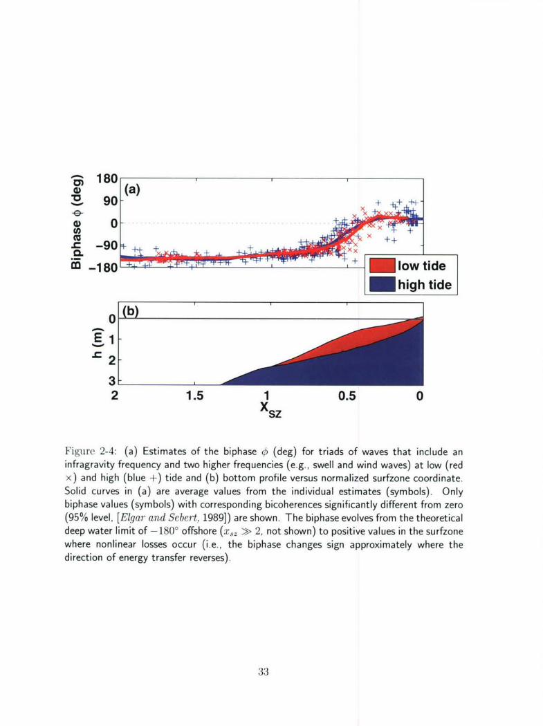
Figur 2-4:()Etmte8ftebpas0dg o trad of waves thtinlde a

x) and~~~~ ~ ~ high (bu )tidean(bbotmpoievrunomlzdsfoecodnt.

Xszý

Solid curves in (a) are average values from the individual estimates (symbols). Onlybiphase values (symbols) with corresponding bicoherences significantly different from zero(95% level, [Elgar' and Se~bert, 19891) are shown. The biphase evolves from the theoreticaldeep water limit of -18O° offshore (xsz »> 2, not shown) to positive values in the surfzonewhere nonlinear losses occur (i.e., the biphase changes sign approximately where thedirection of energy transfer reverses).

33

at most a 20% contribution from bottom friction and other loss mechanisms (assuming

a perfect flux budget). The model results are insensitive to reductions in the bottom

drag coefficient from the nominal [ Wuijanto and Kobayashi, 1991, Raubenhc'imnci et

al., 1995] value Cd = 0.015. In contrast, in model tests with much larger bottom

drag (Cd = 0.05, 0.15), bottom dissipation dominates the energy balance, and a tidal

modulation is not predicted. Thus, in the numerical model, tidal modulation is caused

by differences in nonlinear energy transfers over the low- and high-tide bottomn profiles

(Figure 2-3c) and not by differences in bottom dissipation.

2.3.3 Bottom Profile Dependence

Nonlinear transfers of infragravity energy to motions with higher frequencies were

observed only in water depths less than about 1 in. The triad interactions are closer

to resonance with decreasing depth and require space to transfer energy [Freilich and

Guza, 1984, Herbers et al., 1995b]. Thus, although the total surfzone width does not

change with the tide, the h- 1 dependence of nonlinear triad exchanges (equation 2.2)

predicts enhanced energy transfers over the convex low-tide bottom profile (compared

with the concave high-tide profile), because the horizontal extent (.I h 1 (*)dx) of the

shallow (h < 1 m) region is greater at low tide (Figure 2-3c). The tidal modulation

of infragravity energy observed in 5-m water depth at eight other transects spanning

1.5 km of the coast is consistent with enhanced nonlinear energy transfers over the

convex low-tide profiles (Figure 2-5).

2.4 Conclusions

Observations and numerical model simulations of ocean surface-gravity waves between

15-m water depth and the shoreline show that in the surfzone nonlinear wave-wave

interactions transfer energy from low-frequency (infragravity), long waves to higher-

frequency motions. The energy transfer is enhanced over the relatively flatter iimer-

34

20

18E3

16 high tide

E14

0xS12 X

(U 0 0 x> 10 X X X

X X mid tide 0

00)0 low tide

4- 0

2

0 p I I

0 100 200 300 400 500 600Surfzone f 1/h dx

Figure 2-5: Infragravity variance observed in 5-m water depth versus the integral of h-'across the surfzone at eight transects between y - 1.2 and y = 2.7 km along the coast(including the densely instrumented transect used in the cross-shore analysis). Symbolsare mean values from 50 days of observations at high (blue squares), mid (gray crosses),and low (red circles) tide. The integral over the region where nonlinear losses occur(0 < h < I m) is largest at low tide because the bottom profile is flatter than at hightide.

35

surfzone bottom profile at low tide, explaining the tidal modulation of infragravity

energy observed in bottom-pressure records on the southern California continental

shelf. Similar tidal changes in beach profiles are common worldwide [Woodroffe',

2002, § 6.2.2], and thus tidal modulation of infragravity energy in the surfzone may

affect nearshore processes and regional seismic activity in many areas.

36

Bibliography

Battjes, J.A., H.J. Bakkenes, T.T. Janssen, and A.R. van Dongeren (2004), Shoaling

of subharmonic gravity waves, J. Geophys. Res., 109, C02009,

doi: 10.1029/2003JC001863.

Bowen, A. and R.A. Holman (1989), Shear instabilities of the mean longshore cur-

rent, 1. Theory, J. Geophys. Res., 94, 18023-18030.

Dolenc, D., B. Romanowicz, D. Stakes, P. McGill, and D. Neuhausser (2005), Obser-

vations of infragravity waves at the Monterey ocean bottom broadband station

(MOBB), Geochem. Geophys. Geosys., 6 (9), Q09002,

doi: 10.1029/2005GC000988.

Elgar, S. and R.T. Guza (1985), Observations of bispectra of shoaling surface gravity

waves, J. Fluid Mech., 161, 425-448.


Observations of infragravity waves, J. Geophys. Res., 97, 15573-15577.

Elgar, S., T.H.C. Herbers, and R.T. Guza (1994), Reflection of ocean surface waves

from a natural beach, J. Phys. Oceanogr., 24, 1503-1511.

Elgar, S. and Sebert, G. (1988), Statistics of bicoherence and biphase, J. Geophys.

Res., 94, 10993-10998.

Freilich, M.H. and R.T. Guza (1984), Nonlinear effects on shoaling surface gravity

waves, Proc. Roy. Soc. Lond., A311, 1-41.

Guza, R.T. and E. Thornton (1985), Observations of surf beat, J. Geophys. Res.,

90, 3161-3172.

Hasselmann, K., W. Munk, and G. MacDonald (1963), Bispectra of ocean waves, in

Time Series Analysis, edited by M. Rosenblatt, pp: 125-139, John Wiley, NY.

37

Henderson, S.M. and A.J. Bowen (2002), Observations of surf beat forcing and dis-

sipation, J. Geophys. Res., 107 (ClI), 3193-3203, doi:10.1029/2000JC000498.

Henderson, S.M., R.T. Guza, S. Elgar, T.H.C. Herbers, and A.J. Bowen, Nonlinear

generation and loss of infragravity wave energy, J. Geophys. Res., submitted,

2006.

Herbers, T.H.C. and M.C. Burton (1997), Nonlinear shoaling of directionally spread

waves on a beach, J. Geophys. Res., 102, 21101-21114.

Herbers, T.H.C., S. Elgar, R.T. Guza, and W. O'Reilly (1995a), Infragravity-frequency

(0.005-0.05 Hz) motions on the shelf, II, Free waves, J. Phys, Oceanog., 25,

1063-1079.

Herbers, T.H.C., S. Elgar, and R.T. Guza (1995b), Generation and propagation of

infragravity waves, J. Geophys. Res., 100, 24863-24872.

Herbers, T.H.C., N.R. Russnogle, and S. Elgar (2000), Spectral energy balance of

breaking waves within the surf zone, J. Phys. Oceanogr, 30, 2723-2737.

Herbers, T.H.C., M. Orzech, S. Elgar, and R.T. Guza (2003), Shoaling transforma-

tion of wave frequency-directional spectra, J. Geophys. Res., 108.

Holman, R.A. and A.J. Bowen (1982), Bars, bumps and holes: Models, J. Geophys.

Res., 87, 12749-12765.

Huntley, D., R.T. Guza, and E.B. Thornton (1981), Field observations of surf beat,

1. Progressive edge waves, J. Geophys. Res., 86, 6451-6466.

Janssen T.T., J.A. Battjes, and A.R. van Dongeren (2003), Long waves induced by

short-wave groups over a sloping bottom, J. Geophys. Res., 108 (C8), 3252-

3266, doi:10.1029/2002JC001515.

38

Kobayashi, N. and E. Karjadi (1996), Obliquely incident irregular waves in surf and

swash zones, J. Geophys. Res., 101, 6527-6542.

Lippmann, T.C., T.H.C. Herbers, and E.B. Thornton (1999), Gravity and shear

wave contributions to nearshore infragravity motions, J. Phys. Oceanogr., 29,

231-239.

Longuet-Higgins, M. and R. Stewart (1962), Radiation stress and mass transport in

gravity waves, with application to "surf beats," J. Fluid Mech, 13, 481-504.

Munk, W., F. Snodgrass, and G. Carrier (1956), Edge waves on the continental shelf,

Science, 123, 127-132.

Norheim, C.A., T.H.C. Herbers, and S. Elgar (1998), Nonlinear evolution of surface

wave spectra on a beach, J. Phys. Oceanogr., 28, 1534-1551.

Okihiro, M. and R.T. Guza (1995), Infragravity energy modulation by tides, J.

Geophys. Res., 100, 16143-16148.

Oltinan-Shay, J. and R.T. Guza (1987), Infragravity edge wave observations on two


Oltman-Shay, J., P. Howd, and W. Birkeimeir (1989), Shear instability of the mean

longshore current, 2. Field observations, J. Geophys. Res., 94, 18031-18042.

Peregrine, D.H. (1967), Long waves on a beach, J. Fluid Mech., 27, 815-827.

Raubenheimer, B., R.T. Guza, S. Elgar, and N. Kobayashi (1995), Swash on a gently

sloping beach, J. Geophys. Res., 100, 8751-8760.

Rabinovich, A. and F. Stephenson (2004), Longwave measurements for the coast of

British Columbia and improvements to the tsunami warning capability, Natural

Hazards, 32, 313-343.

39

Rhie, J. and B. Romanowicz (2004), Excitation of Earth's continuous free oscillations

by atmosphere-ocean-seafloor coupling, Nature, 431, 552-556.

Sheremet, A., R.T. Guza, S. Elgar, and T.H.C. Herbers (2002), Observations of

nearshore infragravity waves: seaward and shoreward propagating components,

J. Geophys. Res., 107 (C8), 3095, doi:10.1029/2001JC000970.

Tanimoto, T. (2005), The oceanic excitation hypothesis for the continuous oscillation

of the Earth, Geophys. J. Int., 160, 276-288.

Thomson, J., S. Elgar, B. Raubenheimer, T.H.C. Herbers, and R.T. Guza (2006),




Lon., A202, 565-573.

Van Dongeren, A.P., J. Van Noorloos, K. Steenhauer, J. Battjes, T. Janssen, and

A. Reniers (2004), Shoaling and shoreline dissipation of subharmonic gravity

waves, Int. Conf. Coastal Eng., 1225-1237.

Webb, S., X. Zhang, and W. Crawford (1991), Infragravity waves in the deep ocean,

J. Geophys. Res., 96, 2723-2736.

Woodroffe, C.D. (2002), Coasts: form process and evolution, Cambridge Univ. Press,

New York.

Wurjanto, A. and N. Kobayashi (1991), Numerical model for random waves on

impermeable coastal structures and beaches, Res. Rep. CA CR-91-05, Cent.

for Appl. Coastal Res., Univ. of Delaware, Newark.

40

Chapter 3

Reflection and tunneling of ocean

waves observed at a submarine

canyon

Parts of this chapter were reprinted with permission from:

Thomson, J., S. Elgar, and T.H.C. Herbers (2005),

Reflection and tunneling of ocean waves observed at a submarine canyon,

Geophys. Res. Lett., 32, L10602, doi:10.1029/2005GL022834.

Copyright 2005, American Geophysical Union.

Abstract

Ocean surface gravity waves with periods between 20 and 200 s were observed toreflect from a steep-walled submarine canyon. Observations of pressure and velocityon each side of the canyon were decomposed into incident waves arriving from distantsources, waves reflected by the canyon, and waves transmitted across the canyon. Theobserved reflection is consistent with long-wave theory, and distinguishes betweencases of normal and oblique angles of incidence. As much as 60% of the energyof waves approaching the canyon normal to its axis was reflected, except for wavestwice as long as the canyon width, which were transmitted across with no reflection.Although waves approaching the canyon at oblique angles cannot propagate overthe canyon, total reflection was observed only at frequencies higher than 20 mHz,with lower frequency energy partially transmitted across, analogous to the quantumtunneling of a free particle through a classically impenetrable barrier.

41

3.1 Introduction

Surface waves with periods between 20 and 200 s (deep water wavelengths between

about 500 and 50,000 m) are important to a range of geophysical processes. These

infragravity motions are observed in seafloor pressure signals in deep [Webb et al.,

1991], coastal [Munk et al., 1956, Tucker, 1950], and nearshore [Guza and Thornton,

1985, Elgar et al., 1992] waters. Recent observations suggest that infragravity waves

force resonant oscillations in the earth's crust [Rhie and Romanowicz, 2004], deform

ice sheets [Menemenlis et al., 1995], and can be used as proxies to detect tsunamis

[Rabinovich and Stephenson, 2004]. Much of the infragravity energy in the ocean is

generated nonlinearly by swell and wind waves in shallow water [Longuet-Higgins and

Stewart, 1962, Herbers et al., 1995] and reflected seaward at the shoreline [Elgar et

al., 1994]. Close to the shoreline, infragravity waves can contain more than 50% of the

energy of the wave field [Guza and Thornton 1985], drive shallow water circulation

[Kobayashi and Karjadi, 1996], and affect shoreline sediment transport and nmorpho-

logical evolution [Guza and Inman, 1975, Werner and Fink, 1993]. Consequently,

models for nearshore processes must account for the generation, propagation, and

dissipation of infragravity waves. Here, the strong effect of abrupt shallow water

topography (Figure 3-1) on infragravity wave propagation is shown to be consistent

with theoretical predictions [Kirby and Dalrymple, 1983], and thus can be included

in models for coastal waves, currents, and morphological evolution.

3.2 Theory

The reflection and transmission of long waves (L/h >> 1, where L is the wavelength

and h is water depth) at a long, rectangular submarine canyon of width W are given

by [Kirby and Dalrymple, 1983]

R 2 _ ,T 2 _ 1 (3.1)

42+,"l + '

42

0.0 0

tN -10-0.2

-20-0.4 L ol

30

-0.6 4Wl 40

-0.8 50E

>,-1.0 60

70

-1.280

90

-1.6 ,100

-2.0 -1.8 -1.6 -1.4 -1.2 -1.0 -0.8 -0.6 -0.4 -0.2x (km)

Figure 3-1: Detailed bathymetry (shaded contours) and adjacent coast (tan region) neara steep-walled submarine canyon on the Southern California coast. The La Jolla canyon(dark region) is approximately 115 m deep and 365 m wide, and the surrounding shelfis approximately 20 m deep. The circles on either side of the canyon are locations ofpressure gages and current meters mounted 1 m above the seafloor for 4 weeks duringfall of 2003.

43

and 212 212 2

(' h -2-hCc) sin 2 (1W), (3.2)

where Rf2 and T 2 are the ratios of reflected and transmitted energy, respectively, to

the incident energy, and energy is conserved such that Rf2 + T 2 = 1. The cross-canyoll

components of the wavenumber vector in water depths within (he) and outside (h,)

the canyon are given by Ic and 1, respectively. Assuming Snell's law [Mei, 1989], the

along-canyon component (in) does not change as waves propagate across the canyon.

The dependence of the wavenumber magnitude (k = 27r/L) on wave radian frequency

(w) and water depth (h) is given by the shallow water dispersion relation, W = k V/7Th,

where g is gravitational acceleration.

When waves arrive nearly perpendicular to the axis of the canyon (i.e., normal

incidence), the cross-canyon wavenumber 1, k -m 2 is real (i.e., k,. > ni), and

free wave solutions exist both within and outside of the canyon. For normal incidence,

the amount of reflection depends primarily on the width of the canyon relative to the

wavelength (Eq. 3.2). For example, for a rectangular canyon with h = 20 In, h/,, =

115 m, and W = 365 m (similar to La Jolla Canyon, Figure 3-1), Eqs. 3.1 and 3.2

predict that reflection increases from zero to half of the incident energy as wavelengths

decrease from about 2400 (frequency of 6 mHz) to 600 in (23 mHz) (Figure 3-2a).

Normally incident waves with wavelengths that are integer multiples of twice the

canyon width (W) are transmitted completely across the canyon (e.g., Figure 3-2a,

where R2 = 0 and T2 = 1 for 40 mHz waves [L, - 730 m] normally incident to La

Jolla Canyon [W = 365 m]). The absence of reflection is the result of a standing wave

pattern between the canyon walls that is in phase with the incident waves, allowing

the amplitude at the far side of the canyon to equal the amplitude at the near side

of the canyon [Mei, 1989, Meyer, 1979].

In contrast, if waves approach the canyon axis obliquely, defined here as k, < 'i, so

that k- M2 is imaginary, then no free wave solution exists in the deep water

over the canyon, and nearly all the incident energy is reflected (Figure 3-2b). In the

44

Period (s)178 80 52 38 30 25 21

1 1 1

(a) Normal0.8 I Incidence

0.6

0.4

0.2

0

1

0.8

0.6-

0.4-t

0.2 ObliqueIncidence

6 12 19 26 33 40 47Frequency (mHz)

Figure 3-2: Reflection coefficients R 2 versus frequency (mHz) and period (s) for (a)normally and (b) obliquely incident waves. The curves are based on linear long-wavetheory [Kirby and Dalrymple, 1983] for a rectangular approximation of the canyon cross-section with depth h = 115 m and width W = 365 m. Theory curves are similar forother rectangular approximations of the canyon profile that preserve the cross-sectionalarea, and also are similar over the range of angles in each category (i.e., normal andoblique). Circles are the averages of the 50 total nonlinear inverse estimates of R2 ateach frequency and vertical lines are ± one standard deviation of the estimates. Prior toaveraging over cases of normal incidence (typically about 20 cases) or cases of obliqueincidence (typically about 30 cases), individual R2 values are weighted by the narrownessof the corresponding directional spectrum, such that R2 for narrow directional spectra areweighed more heavily than R 2 for broad spectra.

45

long-wave approximation, the critical angle for total reflection, 101 = arcsin (I),is independent of frequency. For the rectangular idealization of La Jolla Canyon

(Figure 3-1), 101 6 25'. However, for wavelengths (L,) greater than about 1600 in

(i.e., frequencies less than about 20 mHz in Figure 3-2b), a decaying (i.e., evanescent)

wave over the finite-width canyon excites a free wave at the far side of the canyon

[Mass, 1996], resulting in partial transmission of wave energy (Figure 3-3a).

The reflection and transmission of wave energy at the canyon (Figure 3-3a) is

equivalent to "frustrated total internal reflection" in optics and particle tunneling

in quantum mechanics [Krane, 1996, §5.7]. For example, the solution for the quail-

turn tunneling of a free particle with energy E through a potential energy barrier of

amplitude U and width W (Figure 3-3b) can be written by replacing Eq. 3.2 with

u2 sn2 (27fV) (3.)4E(E - U) sin2

where A is the de Broglie wavelength of the particle. The resulting reflection and

transmission coefficients (Eq. 3.1) describe the probability of observing the particle on

either side of the barrier. To the wavelike properties (e.g., A) of the quantum particle,

the barrier acts as a one-dimensional finite-width change in refractive mediium [Kranc,

1996]. When the energy of the particle is greater than tie energy of the barrier

(E > U), the particle may propagate across the barrier, similar to a wave of normal

incidence (k, > m) propagating across the canyon. In contrast, when E < U, the

barrier is classically impenetrable, similar to a wave approaching the canyon at an

oblique (k, < m) angle. Although a particle with E < U cannot be observed within

the barrier region, there is a nonzero probability of observing the particle across the

barrier when the de Broglie wavelength (A) is large compared to the width of the

barrier (analogous to the partial transmission of obliquely incident waves across a

finite-width submarine canyon).

46

(a)Sincident

E 00-C1 00J

-200 re I600

oM 0 30060

)200 -300y (M)

(b)

I-4'J

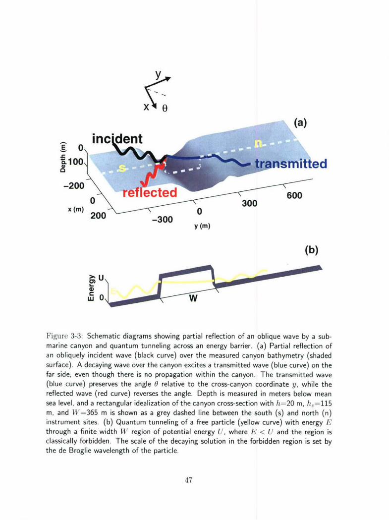
Figure 3-3: Schematic diagrams showing partial reflection of an oblique wave by a sub-marine canyon and quantum tunneling across an energy barrier. (a) Partial reflection ofan obliquely incident wave (black curve) over the measured canyon bathymetry (shadedsurface). A decaying wave over the canyon excites a transmitted wave (blue curve) on thefar side, even though there is no propagation within the canyon. The transmitted wave(blue curve) preserves the angle 0 relative to the cross-canyon coordinate y, while thereflected wave (red curve) reverses the angle. Depth is measured in meters below meansea level, and a rectangular idealization of the canyon cross-section with ih=20 m, hC=115m, and W=365 m is shown as a grey dashed line between the south (s) and north (n)instrument sites. (b) Quantum tunneling of a free particle (yellow curve) with energy Ethrough a finite width W region of potential energy U, where E < U and the region isclassically forbidden. The scale of the decaying solution in the forbidden region is set bythe de Broglie wavelength of the particle.

47

3.3 Field Observations

To test Eqs. 3.1 and 3.2 in the ocean, measurements of surface-wave-induced pressure

and velocity were made with colocated sensors deployed in 20-mn water depth (tide

range about 1 m) approximately 200 m north and 100 in south of La Jolla Submarine

Canyon, near San Diego, California (Figure 1) for 4 weeks during the fall of 2003.

Infragravity wave (5 to 50 mHz) significant heights (4 times the sea-surface elevation

standard deviation) ranged from 0.01 to 0.20 m. Reflection coefficients were esti-

mated from the 50 (of 327 total) two-hr long time series (sampled at 1000 mHz) with

infragravity significant heights greater than 0.05 m at both sides of the canyon. For

records with significant heights below 0.05 m, estimates of reflection coefficients may

by contaminated by noise in the pressure and velocity measurements.

In contrast to the unidirectional waves used in a laboratory investigation of Eqs.

3.1 and 3.2 [Kirby and Dalrymple, 1983], ocean waves can have broad directional

distributions that differ on each side of the canyon. The random wave fields on

the north (n) and south (s) sides of the canyon consist of incident, reflected, and

transmitted (from the other side of the canyon) waves (Figure 3-3a), such that the

surface elevations q, and ?In can be written as integrals over wave components at each

frequency and direction, given by

2.JJS 2 d. (ei(mx+1Y-wt) + Rei(mx-Ivwt +0)) + dn (Tnet(mx-1~Y-wt)) (3.4)2

77n 2 dn (ei(mx-IYwt) •Rned(mx+-lY-wt±Vn)) + ds (Tsei("tx vY-wt)) (3.5)=-2

where ds and dn are the complex-valued differential amplitudes of the incident wave

components at radian frequency w and direction 0 relative to the local cross-canyon

coordinate y. The variables Rs, Rn, Ts, and Tn are reflection and transmission coef-

ficients, 7P, and 7P,, are the phase shifts of the reflected waves relative to the inIcident

waves, x is the local along-canyon coordinate, and t is time. Reflection is assumed

48

to be specular, and thus the sign of the cross-canyon wavenumber (1 = k cos 0) is re-

versed upon reflection, while the sign of the along-canyon wavenumber (m = k sin 0)

is preserved (Figure 3-3a). In this two-quadrant (--' < 0 < -) system, the direction2 2

of y propagation is given explicitly by the sign of the exponent in elly because 1 is

always positive.

3.4 Methods

In contrast to methods used to estimate the amount of reflection from impermeable

structures [Dickson et al., 1995], estimation of the reflection of a canyon must also

account for transmission. Here, inverse techniques [Coleman and Li, 1996] are used

to determine the reflection (R,, Rn) and transmission (T,, Tn) coefficients, as well as

the incident directional spectra (D,, Dn) and reflected phases (0,, On) of the wave

fields on the south (s) and north (n) sides of the canyon that are most consistent with

observations of pressure and velocity.

The cross-canyon velocity v, along-canyon velocity u, and pressure p fields induced

by surface waves (Eqs. 3.4 and 3.5) can be determined from a linear, hydrostatic

momentum balance (appropriate for infragravity waves in 20-ni water depth) given

byOv ',7a OU O7

t-g y & - -gax P= Pg97, (3.6)

where g is gravitational acceleration and p is density.

Substituting 77, and 7in into the momentum balance (Eq. 3.6), using the Fourier

transformed result, and applying the identities 2i sin(ia) = e- 0 - ea and 2 cos(ia) =

ea + e-a yields the following expressions for the frequency cross-spectra of the colo-

cated pressure and velocity time series south (s) of the canyon

(ps(w) .u*(W'))=pgj sin0 [DPTn2 + Ds (I + R2 + 2Rs cos 0,)] dO, (3.7)

49

(Ps(w).v:(W))=Pgtccoso -_DT ± •D (1- +R i2RsinP)] dO, (3.8)

(Us(W) Vs(W))= K2jsin0cos0 [-- ±2 D, (1--2±i2Rsin0)] dO, (3.9)

where r, = 9 * is the complex conjugate, and () is the expected value. Similarly,

the auto-spectra are

(ps(W).p;*(w))=(pg)2o [DnT2 + Ds (1 + R2 + 2Rs cos 0,s)] dO, (3.10)

(us(W).u*(W))=K2 fosin 20 [DT,2 + Dsl (I +R2+ 2Rscos s) dO, (3.11)

(Vs(w).v*2(w))=2f COS2 0 [D 2+ D (1 + R 2- 2R, sin'•Vs)] dO, (3.12)

The incident wave directional spectra D, and D, are defined as

D,(w,O) = <d. d (.13

dwdO

D,,(w, 0)- = dnd) (3.14)

dwdO

The incident wave fields on the north and south sides of the canyon are independent

of each other, and thus (d,. d*) = (dn . d*) = 0.

Expressions for cross- and auto-spectra at the north side of the canyon are obtained

by exchanging all subscripts (s--+n) in the expressions above (Eqs. 3.7-3.12) and

changing the sign of the integrand in Eqs. 3.8 and 3.9.

The real-valued terms describe the progressive wave field, and the imaginary (i)

terms (i.e., the quadrature in the cross-spectra (p.v*) and (u.v*)) describe the partial

standing wave patterns owing to sums of incident and reflected waves. In practice,

the expressions for cross- and auto-spectra apply only to observations near the canyon

walls, because over large distances (i.e., many wavelengths) standing wave patterns

are obscured within a finite-width frequency band.

For computational efficiency, the incident directional spectra (Eqs. 3.13 and 3.14)

50

at each frequency band are modeled as [Donelan et al., 1985]

D,(0) = Mscos2S. ( E) , (3.15)

Dn(0) = M, cos 2Sn ( - ), (3.16)

where E) and E, are the centroidal directions, S, and Sn describe the spread in di-

rection about the centroid, and M, and Mn are the spectral peak values. The results

are insensitive to the specific unimodal shape used for the incident directional spec-

tra. The centroidal directions Es and E) were used to separate the data sets (at

each frequency band) into normally (161 < 200) and obliquely (I01 > 300) incident

waves. Assuming directionally narrow spectra, the reflection (R,, Rn) and transmis-

sion (Ts, T,,) coefficients are assumed to be independent of direction at each frequency.

The p)hase shifts 4', and V), of the reflected waves relative to the incident waves

were allowed to vary over each directional spectrum by a.ssuming

,0(0) = 2Aysk cos 0, (3.17)

V)n(0) = 2AynkcosO, (3.18)

where Ays and Ay, are the (unknown) distances between the reflector and the in-

strument locations (i.e., 4' is the phase change associated with propagating toward

and back from the reflector).

Assuming energy is conserved (i.e., R + T± 2 = 1, R' + T,,2 = 1), tile inverse

method finds the north (n) and south (s) values of E, S, M, R, and Ay that are most

consistent with the cross- and auto-spectra of the observed time series by minimizing

a normalized root-mean-square error [Dickson et al., 1995]

r Z(obs - derived) . (obs - derived)* (3.19)1(obs)(obs)*

51

where E is the sum over the six auto- and cross-spectral values from the south side

(Eqs. 3.7-3.12) and the six spectral values from the north side. Applying recent

improvements to Newton's method [Coleman and Li, 1996], the inverse algorithm

begins with an initial guess for each unknown, and solves a locally linearized version

of the equations for the cross- and auto-spectra to find the small change in each

unknown that produces the greatest reduction in c (i.e., the method iterates down-

slope in c until the minimum is found). Initial guesses for E, S, and M are provided

by estimates of directional moments of the wave field based on the measured pressure

and velocities [Kuik et al., 1988], and the initial guesses for R are based oil long-wave

theory [Kirby and Dalrymple, 1983]. The results (Figure 3-2) are not sensitive to the

initial values, and the same inverse solutions are obtained with random initial guesses

(although computational time is increased).

3.5 Results

For waves normally incident to the canyon axis, reflection coefficients estimated with

the inverse method are consistent with long-wave theory (Figure 3-2a), including

the nearly complete transmission of waves with wavelength twice the canyon width

(W = 365 in, L, ; 730 m, frequency = 40 mHz). When unidirectional waves are

normally incident on each side of the canyon (i.e., symmetric normal incidence),

a forward calculation can be used to estimate reflection, and the few cases that

satisfied these criteria also are consistent with long-wave theory (not shown). Inverse

estimates of reflection coefficients for waves obliquely incident to the canyon axis also

are consistent with theory, including the nearly complete reflection of waves with

frequencies above about 20 mHz, and the tunneling that results in reduced reflection

of lower frequency waves (Figure 3-2b).

The observed reflection of obliquely incident waves is somewhat less than theoret-

ical predictions (Figure 3-2b), possibly because the neglected non-uniformity of the

52

La Jolla Canyon profile (Figure 3-1) becomes increasingly important as the incidence

angle increases. The reduction in the sharpness of the canyon results in reduced re-

flection, and also may contribute to the scatter within the reflection coefficients at

each frequency band (Figure 3-2). Directionally spread wave fields that simultane-

ously contain energy at both normal and oblique angles likely increase the scatter. To

reduce this effect, the spreading parameters (Ss, Sn) were used to weight individual

estimates of R 2 by

R2vg SsR nSn12 (3.20)E S. +• Sn

to calculate an average value R2vg at each frequency from the collection of data runs

(e.g., the symbols in Figure 3-2).

Statistical fluctuations in the cross-spectra of finite-length data records may pro-

duce additional scatter in the results [Wunsch, 1996], and the residual errors (Eq.

3.19) approximately follow the expected X2 distribution of such fluctuations. The

percent of observed variance captured by the inverse method (defined as 100 x [1 -c2])

is 90% when averaged over all infragravity frequency bands for all 50 data sets.

Estimates of the phase differences 0, and oin between incident and reflected waves

are consistent with the travel time required for a wave to propagate to the reflector

and back (Figure 3-4), providing a consistency check on the inverse solutions. The

small deviations from theoretical phase shifts may be owing to errors in approximating

the sloped canyon walls as vertical. Further investigation of the reflected wave phase

lags could be used to investigate the effect of a spatially distributed reflector (e.g.,

reflection by sloping, irregularly shaped walls). Alternatively, the inverse method

could be restructured as an over-determined set of equations by specifying V), and V),

as known from measurements of Ay, and AyN (i.e., assuming Eqs. 3.17 and 3.18 are

valid), but at the expense of being able to verify the solutions.

53

Period (s)

178 80 52 38 30 25 21300 1......

(a) South

200-

0 OOOOOOM< 100

0~~ T0

300(b) North

< 100

6 12 19 26 33 40 47Frequency (mHz)

Figure 3-4: Distance (m) between the reflector and the instrument location versus fre-quency (mHz) and period (s) at the (a) south and (b) north sides of the canyon. Symbolsare estimates from the nonlinear inverse method and solid lines are the measured dis-tances from the steepest portion of each canyon slope to the instrument site at that side.Instrument locations were determined within ± 10 m (the width of the solid lines) withdifferential GPS. The theory assumes that waves propagate from the instrument site to avertical-canyon-wall reflector along a line of constant y and back, neglecting possible phaseshifts at the sloped walls. Vertical lines are ± one standard deviation of the estimates.

54

3.6 Conclusions

During the 4-week observational period, on average more than half the incident in-

fragravity wave energy was reflected by La Jolla submarine canyon. Although low

frequency (less than about 20 mHz) waves arriving at angles oblique to the canyon axis

cannot propagate within the canyon, a tunneling phenomenon predicts that reflection

is only partial (i.e., some energy is transmitted across the canyon), consistent with

the observations. These results suggest that reflection of directionally spread waves

by complex shallow water bathymetry should be included in models of nearshore

processes and considered as a potential shore protection method.

55

Bibliography

Coleman, T. and Y. Li (1996), An interior, trust region approach for nonlinear

minimization subject to bounds, SIAM J. Optimization, 6, 418-445.

Dickson, W., T.H.C. Herbers, and E. Thornton (1995), Wave reflection from break-

water, J. of Water., Port, Coast., Ocean Eng. 121, 262-268.

Donelan, M., J. Hamilton, and W. Hui (1985), Directional spectra of wind-generated

waves, Phil. Trans. Roy. Soc. Lon., A 315, 509-562.

Elgar, S., T.H.C. Herbers, M. Okihiro, J. Oltman-Shay, and R. Guza (1992), Ob-

servations of infragravity waves, J. Geophys. Res., 97, 15573-15577.

Elgar, S., T.H.C. Herbers, and R.T. Guza (1994), Reflection of ocean surface waves

from a natural beach, J. Phys. Oceanogr., 24, 1503-1511.

Guza, R.T. and D. Inman (1975), Edge waves and beach cusps, J. Geophys. Rcs.,

80, 2997-3012.

Guza, R.T. and E. Thornton (1985), Observations of surf beat, J. Geophys. Res.,

90, 3161-3172.

Herbers, T.H.C., S. Elgar, and R. Guza (1995), Generation and propagation of

infragravity waves, J. Geophys. Res., 100, 24863-24872.

Kirby, J. and R. Dalrymple (1983), Propagation of obliquely incident water waves

over a trench, J. Fluid Mech., 133, 47-63.

Kobayashi, N. and E. Karjadi (1996), Obliquely incident irregular waves in surf and

swash zones, J. Geophys. Res., 101, 6527-6542.

Krane, K. (1996), Modern Physics, 2nd ed., John Wiley & Sons, New York.

56

Kuik, A., G. Van Vledder, and L. Holthuijsen (1988), A method for the routine

analysis of pitch-and-roll buoy wave data, J. Phys. Oceanogr. 18, 1020-1034.

Longuet-Higgins, M. and R. Stewart (1962), Radiation stress and mass transport in

gravity waves, with application to "surf beats," J. Fluid Mech., 13, 481-504.

Maas, L.R.M. (1996), Topographic filtering and reflectionless transmission of long

waves, J. Phys. Oceanogr., 27, 195-202.

Mei, C.C. (1989), The Applied Dynamics of Ocean Surface Waves, World Scientific,

New Jersey.

Menemenlis, D., D. Farmer, and P. Czipott (1995), A note on infragravity waves in

the Arctic ocean, J. Geophys. Res., 100, 7089-7094.

Meyer, R.E. (1979), Surface wave reflection by underwater ridges, J. Phys. Oceanogr.,

9, 150-157.

Munk, W., F. Snodgrass, and G. Carrier (1956), Edge waves on the continental shelf,

Science, 123, 127-132.

Rabinovich, A. and F. Stephenson (2004), Longwave measurements for the coast of

British Columbia and improvements to the tsunami warning capability, Natural

Hazards, 32, 313-343.





doi: 10. 1029/2005GL022834.


Lon., A 202, 565-573.

57


J. Geophys. Res., 96, 2723-2736.

Werner, B. and T. Fink (1993), Beach cusps as self-organized patterns, Science, 260,

968-971.

Wunsch, C. (1996), The Ocean Circulation Inverse Problem, Cambridge University

Press, Cambridge.

58

Chapter 4

Conclusions and Regional

Description

The primary result of this thesis research is an improved understanding of the effects

of bottom topography on the propagation of infragravity waves. Depending on the

bottom profile, in shallow water (h < 3 m) nonlinear interactions with swell and

wind waves result in net energy transfer to or from infragravity waves [Thomson et

al., 2006]. In deeper water (h > 3 m), infragravity waves are partially reflected from,

and partially transmitted across, a steep-walled canyon, consistent with linear long-

wave theory [Thomson et al., 2005]. In addition, the extensive field observations can

be used to investigate the regional propagation of infragravity waves. In particular,

the results can be combined with refraction models to simulate the propagation of

infragravity waves over complex shallow water bathymetry.

4.1 Shoaling and Unshoaling

Studies on several beaches have found that infragravity motions are predominantly

cross-shore oriented [Guza and Thornton, 1985, Sheremet et al., 2002, Reniers et al.,

2006], and thus cross-shore approximations, as in Chapter 2, are common to many in-

59

fragravity analyses. The NCEX observations are consistent with this approximation,

because, on average, alongshore motions contributed only 20% of the total infragravity

velocity variance. In addition, at the nearby Torrey Pines State Beach (y = 3.0 kin,

Figure 1-3), alongshore propagating edge waves detected in shallow (h < 3 in) wa-

ter contained only 15% of the total infragravity pressure variance [Oltman-Shay and

Guza, 1987]. However, at offshore locations (h > 5 m, jxj > 500 m, Figure 1-3),

NCEX observations of infragravity velocities were closer to isotropic (alongshore nmo-

tions were 40%, oil average, of the total velocity variance), consistent with previous

observations of cross-shore dominated wave fields that became directionally broader

during seaward refraction [Herbers et al., 1995b].

Similar to previous results, NCEX observations of total infragravity energy across

the shelf (Figure 4-1) are consistent with freely propagating waves that shoal and

unshoal within the theoretical limits of h- 112 for cross-shore propagating waves [El-

gar et al., 1992, Figure 3] and h- 1 for isotropic edge waves [Herbers et al., 1995a,

Figure 7]. Contributions from forced, or group bound, waves that shoal proportional

to a theoretical maximum h- 5 [Longuet-Higgins and Stewart, 1962] are small every-

where except the surfzone. Seaward propagating free waves are a significant portion

of the total infragravity energy (e.g., Figure 2-2), and unshoal during refraction over

the bathymetry.

4.2 Refraction and Canyon Reflections

The propagation of swell outside the surfzone is modeled accurately by the refraction

of energy-flux conserving rays [Munk and Traylor, 1947, O'Reilly and Guza, 1993;

and many others]. Here, a refraction model is presented that describes the seaward

radiation of infragravity waves and accounts for partial reflections and transmissions

at the Scripps and La Jolla canyons. The model is initialized with observations in

2.5 in depth (nominally outside the surfzone), assuming half the variance is radiated

60

103

. data (hourly)

best fit1/2

- free waves (h-)

"- - - free waves (h-5

E" ....... bound waves(h

010X X

>

L 0"10

/

--1 0 1__ 211 0 . . . . .. . . . .. ... . ... . . .

10- 100 101 102

Infragravity energy (cm 2) at h = 15 m

Figure 4-1: Infragravity energy (cm 2 ) observed at h = 15 m versus infragravity energy(cm 2 ) observed at h = 5 m along the northern transect (y = 2.7 km, Figure 1-3). Theleast squares linear fit (solid line, slope = 2.4, correlation = 0.95) to the hourly data(symbols) is between the theoretical h-1 / 2 shoaling of cross-shore propagating free waves(lower dashed line, slope = (5/15)-1/2 = 1.7) and the theoretical h-' shoaling of isotropicfree edge waves (upper dashed line, slope = (5/15)-i = 3). The observations are far fromthe theoretical h-s shoaling of cross-shore propagating forced waves (dotted line, slope= (5/15)-5 = 243). Some spread is expected owing to tidal fluctuations (1 m), whichchange ratios of instrument depths slightly (but not the absolute difference in depth),

such that (15±1 ) •1/2 ± 1.7±0.1 and ( 5±1) = 3.0±0.2.

61

seaward (e.g., reflection coefficient R 2 = 1). Subsequent reflections of energy that

returns to the shoreline (along refractively trapped rays) are neglected.

Rays are traced [original code by M. Orzech, Naval Postgraduate School] using

Xn+1 = x, +dscos(On) and yn+l = y. +dssin(0,) (4.1)

where x and y refer to the NCEX grid (Figure 1-3), n is the integer number of ray

segments along a ray path, ds is the length (5 m) of a ray segment, and the angle 0

is determined by [Mei, 1989, §3.2]

0.+1 = 0. + I sin(On) -cos(On) 0 , (4.2)

using the local depth h = h(xn, Yn). Initial angles, 00, are obtained from the ob-

servations or are prescribed. The partial reflections and transmissions are predicted

by Eqs. 3.1 and 3.2, using rectangular approximations of the canyon cross-sections.

Energy flux is conserved along each ray by shoaling and unshoaling proportional to

h- 1/ 2 . Energy flux also is conserved at each canyon where incident rays are split into

reflected (at specular angles) and transmitted (angle conserved across the canyon)

portions that continue to refract until returning to the surfzone (re-reflections at the

shoreline are neglected) or reaching the deep water beyond the shelf. For example,

ray paths of 50 s period infragravity waves propagating seaward from 2.5 in depth at

an initial angle 00 = -20' from shore normal are partially reflected by Scripps canyon

(Figure 4-2), reducing the amount of wave energy that propagates southward along

the shelf and refracts back to the shoreline.

To study the regional distribution of infragravity waves, ray paths are calculated

for all possible frequencies (0.0068 Hz resolution) and initial angles (50 resolution)

from the 2.5 m isobath. Each ray is assigned an initial relative energy flux F and

direction 00 based on observations in 2.5 m depth, using the unimodal directional

spectrum given by Eqs. 3.15 and 3.16, and interpolated to evenly spaced (50 mn)

62

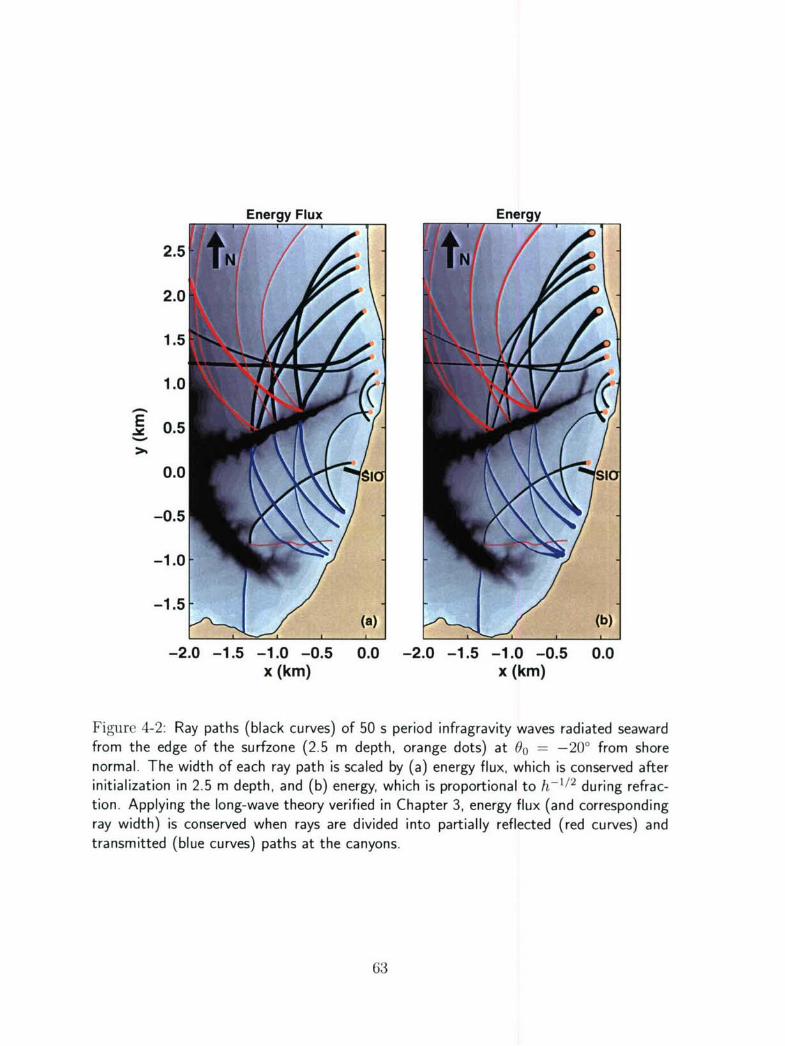
Energy Flux Energy

2.5)

2.0

1.5

1.0

.• 0.5

0.0 SGS

-0.5

-1.0

-2.0 -1.5 -1.0 -0.5 0.0 -2.0 -1.5 -1.0 -0.5 0.0

x (km) x (km)

Figure 4-2: Ray paths (black curves) of 50 s period infragravity waves radiated seawardfrom the edge of the surfzone (2.5 m depth, orange dots) at Oo = -200 from shorenormal. The width of each ray path is scaled by (a) energy flux, which is conserved afterinitialization in 2.5 m depth, and (b) energy, which is proportional to h-1/ 2 during refrac-tion. Applying the long-wave theory verified in Chapter 3, energy flux (and correspondingray width) is conserved when rays are divided into partially reflected (red curves) andtransmitted (blue curves) paths at the canyons.

63

locations along the 2.5 m isobath. Ray paths are traced seaward from 2.5 in depth,

and then summed over a 50-m resolution grid, assuming a linear superposition of the

refracted wave components. Approximating the depth h as constant within each grid

cell, the infragravity variance is calculated by summing contributions E2 Fds(gh)-1/2

of ray segments passing thru each grid cell [Bouws and Battjes, 1982].

The modeled variance distribution is compared with the total infragravity variance

observed at offshore instrument sites (grouped by depth for plotting, Figures 4-3 and

4-4). A normalized root-mean-square error e (Eq. 3.19) is used to compare the

modeled variance with the observed variance (Figure 4-5). The total variance is used

because the dominant contributions to the shelf infragravity wave field are free waves

(e.g., Figure 4-1) generated in the nearby surfzone. Additional free wave energy from

remote sources (e.g., surfzones across the Pacific Ocean [Webb et al., 1991]), as well

as local group-bound contributions, are assumed to be small. Several grid resolutions

(150, 100, 50, 25 m) and ray segment lengths (ds = 5,10,20 in) were tested, with

the final 50 m grid and 5 m ray segment values chosen as the best combination of

accuracy and computational efficiency. The results are insensitive to the type (e.g.,

linear, quadratic, cubic spline) of interpolation used for producing initial conditions.

4.2.1 Case Study

In a case study with narrow-banded directional spectra (Oo = -20 + 15') radiated

seaward from the surfzone, canyon effects (reflection and transmission) are important

to the distribution of infragravity variance (Figure 4-3). If canyon effects are neglected

(i.e., paths include refraction only), the energy flux along paths that intersect the

canyon (e.g., Figure 4-2) is propagated southward along the coast (i.e., not reflected),

and the resulting infragravity variance is overpredicted at most sites (Figure 4-3).

Although as large as a factor of two in places (e.g., y = 1100 m on the 5 in isobath,

Figure 4-3b), the overprediction typically is not severe because Scripps canyon is

narrow (- 100 m wide) relative to infragravity wavelengths (- 500 m), and thus

64

Case 1w reflections:Oct 18-19 - - - no reflections

40 (a) 2.5 m isobath (initial condition) observed

o20-

10

2 0 - .(b ) 5 M .i.. ... . ....... . ........ .

104

E 1 0 . .. . ..... . . . . . . . . .• . . . .

0 i

20 (c) 10 m isobath

.. ~7V " .0

•

20 (d) 15 m isobath

E 10 - ........... . . . . . . . ... . . . -. V V9

0I~ ~ ~~~ WA Yi" i

0-

-1000 -500 0 500 1000 1500 2000 2500 3000y (m)

Figure 4-3: Observed (symbols) and modeled (curves) infragravity variance (cm 2) versusalongshore distance y (m) at four depths h = (a) 2.5, (b) 5.0, (c) 10.0, (d) 15.0 m for12 hrs spanning October 18-19, 2003. In this directionally narrow-banded case study, aray tracing model that includes reflection and transmission at the canyons (solid blackcurves) has more skill than a refraction-only ray tracing model (dashed green curves).The models are initialized by interpolating the observations along the 2.5 m isobath (a)and radiating rays seaward according to the 12 hr averaged 0o = -20 ± 150 directionalspectrum estimate, where 0 is measured relative to shore normal.

65

modeled reflections are small (< 30%) for most angles of incidence (Eq. 3.1). Likely,

canyon effects would be more significant (e.g., reflections up to 95%,) ill the vicinity

of the wider (- 350 nm) La Jolla Canyon, but there were only limited observations for

comparison, and none for surfzone initialization, south of the Scripps Pier (y < 0.0 kin,

Figure 1-3).

4.2.2 Climatology

When averaging over almost two months of data to examine all approximate clina-

tology of infragravity variance in the region surrounding Scripps canyon, the averaged

directional spectrum radiated seaward from the surfzone (i.e., the initial condition)

is broad and symmetric (average 00 = 0 ± 60'), and the corresponding distribution

from the ray tracing model is insensitive to canyon reflection effects (Figure 4-4).

The alongshore gradients of infragravity energy, which are established in tile surf-

zone by the incident swell energy, are reduced during the seaward propagation and

unshoaling of a wave field with broad-band directional spectra (i.e., the curves in

Figure 4-4 become flatter as water depth increases). Thus, the averaged distribution

demonstrates only the indirect effect of the canyons, because refraction of inconiing

swell over the canyons affects the amount of energy available for infragravity wave

generation, but does not affect the averaged outgoing infragravity wave propagation.

Individual ray paths, however, can undergo significant reflections (e.g., Figure 4-2),

and because energy propagating along individual ray paths could be important ill

forcing resonant seiche modes of harbors and bays, reflections should be included in

models of broad-band wave propagation over steep bathymetry.

4.2.3 Model Skill

Comparisons of the observed infragravity variance with model simulations of variance

indicate that reflection and transmission at the canyons are important near Scripps

canyon (Figure 4-5a), but decrease in importance with distance from the canyons

66

Climatology -• w/ reflections- - - no reflections

40 (a) 2.5 m isobath (initial condition) observed

,30-

5 20

100 iiiii

20 (b) 5 M isobath ....

10

20 (c) 10 m isobath .......

E 10

0

20 (d) 15 m isobath ...........

E 10-

0 Vi i ii

-1000 -500 0 500 1000 1500 2000 2500 3000y (m)

Figure 4-4: Average observed (symbols) and modeled (curves) infragravity variance (cm 2)versus alongshore distance y (m) at four isobaths h = (a) 2.5, (b) 5.0, (c) 10.0, (d) 15.0 mfor the entire Nearshore Canyon Experiment (fall 2003). Canyon effects are blurred whenresults are integrated over directionally broad-banded spectra. When initialized with anaveraged frequency-directional spectrum, a ray tracing model that includes reflection andtransmission at the canyons (solid black curves) has skill similar to that of a refraction-only ray tracing model (dashed green curves). The models are initialized by interpolatingthe average variance observed along the 2.5 m isobath (a) and radiating rays seawardaccording to an average 0 = 0 ± 600 directional spectrum estimate, where 0 is measuredrelative to shore normal. Averaging the results from all the individual cases using case-by-case initial conditions results in a similar description of the climatology.

67

h -15 m, y =573 m h =15 m, y 2700 m102 102

S(a ) (b )

E010 10 0

0 0 0)0-100 1000 0

-- 0 1 . * -10 - w

10-2 0 -2

10-2 100 102 10-2 100 10

Observed energy (cm 2) Observed energy (cm 2)

W 2 W(c) ....

0 w/ reflectionsL1.5-1

Sn - - - no reflections

% "

E % S&_ 0.5-s• . s .0 La 1191a Scips " Ss•

0 Canyon, Canyon

-1000 -500 0 500 1000 1500 2000 2500 3000

y (m)

Figure 4-5: Modeled versus observed infragravity energy (cm 2 ) in 15-m water depth

(a) near a canyon and (b) far from the canyons, and (c) normalized root-mean-square

model errors versus alongshore distance. Results from the refraction model with canyon

reflections (black filled circles) are scattered around a 1:1 agreement (gray lines) with

observations at both locations (a and b). Results from the refraction model without

canyon reflections (green open circles) agree with observations at locations far from the

canyons (b), but not at locations near a canyon (a). The depth-averaged normalized root-

mean-square error (c) is small along the entire array for the refraction model with canyon

reflections (black curve), and large in the vicinity of the La Jolla and Scripps canyons for

the refraction-only model (green dashed curve).

68

(Figure 4-5b). Averaging over all 1-hr records (1100 total) and all offshore instrument

locations (40 total), including canyon effects in the refraction simulations results in

improved model skill within one km (i.e., a few wavelengths) of the canyons, where

the normalized model error remains small only if reflection and transmission are

included (Figure 4-5c). On average, the refracted-reflected-transmitted ray tracing

model explains 84% of the observed variance (defined as 100 x [1 - C2]), while the

refraction-only version explains 70% of the variance. Canyon reflection effects are

found to be most significant for cases with narrow-banded initial directional spectra.

For directionally broad-banded wave fields, the energy is spread more evenly over the

ray paths at each grid cell, and the modeled variance distributions are similar with

or without accounting for reflection and transmission at the canyons.

4.3 Suggested Applications

The results presented in this thesis can be used to improve the accuracy of nonlinear

wave models in the surfzone and to extend the validity of linear wave models to

regions of steep topography. The results could be incorporated into a comprehensive

coastal wave model in which:

"* swell waves are refracted shoreward from a single offshore measurement,

"* infragravity wave energy is gained by nonlinear interactions in the shoaling

region,

"* infragravity wave energy is gained and lost by nonlinear interactions in the

surfzone (including tidal modulations owing to variable beach slopes),

"* the resulting total wave energy forces a nearshore circulation and corresponding

sediment transport model,

"* infragravity waves are reflected from the beach and radiated seaward,

69

"* seaward rays are refracted and partially reflected over topography, and

"* the resulting regional infragravity distribution forces bottom-pressure fluctua-

tions (observed in seismic records) and possible harbor and bay resonances.

The improved predictions of infragravity waves within such a comprehensive model

might be of use in coastal engineering and management applications. At present,

the predictions of nearshore conditions that are used for recreational, commercial,

or defense related sites are semi-empirical and remain prone to errors because of

deficiencies in modeling the underlying physics. Infragravity wave dynamics must

be understood before these models can predict nearshore waves, currents, and mor-

phology accurately. For example, infragravity edge waves can support alongshore

pressure gradients [Mei, 1989, § 4.8] that can force circulation patterns, including the

episodic and hazardous seaward flows know as rip currents [MacMahan et al., 2004].

In addition, infragravity motions dominate the run-up of water onto the beach face

[Raubenheimer and Guza, 1996], and are associated with morphological features such

as beach cusps [Ciriano et al., 2005] and flooding during storIns. Farther offshore,

infragravity motions contaminate ocean bottom seismology measurements used to de-

tect tsunamis [Mofjeld et al. 2001] and to predict microseisms [Rhie and Romanowicz,

2004].

In addition to modeling studies and predictive applications, future work might

include investigations of submarine canyons as shoreline protection systems, possible

feedbacks between tidal modulations and nearshore bottom profiles, the momentum

balance associated with the reversal of nonlinear transfers in shallow water, and infra-

gravity wave participation in the overall energy cascade to higher frequencies during

surfzone wave breaking [Herbers et al., 2000].

70

Bibliography

Bouws, E. and J.A. Battjes (1982), A Monte Carlo approach to the computation of

refraction of water waves, J. Geophys. Res., 87, C8 5718-5722.

Ciriano, Y., G. Coco, K.R. Bryan, and S. Elgar (2005), Field observations of swash

zone infragravity motions and beach cusp evolution, J. Geophys. Res., 110,

C02018, doi:10.1029/2004JC002485.

Elgar, S., T.H.C. Herbers, and R.T. Guza (1994), Reflection of ocean surface gravity

waves from a natural beach, J. Phys. Oceanogr., 24, 1503-1511.


Observations of infragravity waves, J. Phys. Oceanogr., 97, C10 15573-15577.

Guza, R.T., and E.B. Thornton (1985), Observations of surf beat, J. Phys. Oceanogr.,

90, C2 3161-3172.

Herbers, T.H.C, S. Elgar, and R.T. Guza (1995a), Infragravity-frequency (0.005-0.05

Hz) motions on the shelf, II, Free waves, J. Phys. Oceanogr., 25, 6, 1063-1079.

Herbers, T.H.C, S. Elgar, and R.T. Guza (1995b), Generation and propagation of

infragravity waves, J. Phys. Oceanogr., 100, C12 24863-24872.

Herbers, T.H.C., N.R. Russnogle, and S. Elgar (2000), Spectral energy balance of

breaking waves within the surf zone, J. Phys. Oceanogr., 30, 2723-2737.

Longuet-Higgins, M.S. and R.W. Stewart (1962), Radiation stress and mass trans-

port in surface gravity waves with application to surf beats, J. Fluid Mech., 13,

481-504.

MacMahan, J.H., A.J.H.M. Reniers, E.B. Thornton, and T.P. Stanton (2004), In-

fragravity rip current pulsations, J. Geophys. Res., 109, C01033,

doi: 10. 1029/2003JC002068.

71

Mei, C.C. (1989), The Applied Dynamics of Ocean Surface Waves, Adv. Series on

Ocean Eng., Vol 1, World Scientific, New Jersey, 740 pp.

Mofjeld, H.O., P.M. Whitmore, M.C. Eble, F.I. Gonzlez, and J.C. Newman (2001),

Seismic-wave contributions to bottom pressure fluctuations in the North Paci-

ficlmplications for the DART Tsunami Array, Proc. Int. Tsunami Sym. 2001

(ITS 2001), Session 5-10, 633641.

Munk, W.H. and Traylor, M.A. (1947), Refraction of ocean waves: a process linking

underwater topography to beach erosion, J. of Geology, LV, 1-26.

Oltman-Shay, J., and R.T. Guza (1987), Infragravity edge wave observations on two


O'Reilly, W.C., and R.T. Guza (1993), A comparison of two spectral wave models

in the Southern California Bight, Coastal Eng., 19, 263-282.

Raubenheimer, B. and Guza, R.T. (1996), Observations and predictions of run-up,

J. Geophys. Res., 101, Cll 25575-25587.

Reniers, A.J.H.M., J.H. MacMahan, E.B. Thornton, and T.P. Stanton (2006), Mod-

elling infragravity motions on a rip-channel beach, Coastal Eng., 53, 209-222.



Sheremet, A., R.T. Guza, S. Elgar, and T.H.C. Herbers (2002), Observations of

nearshore infragravity waves: seaward and shoreward propagating components,

J. Geophys. Res., 107 (C8), 3095, doi:10.1029/2001JC000970.



doi: 10. 1029/2005GL022834.

72

Thomson, J., S. Elgax, B. Raubenheimer, T.H.C. Herbers, and R.T. Guza (2006),




J. Geophys. Res., 96, 2723-2736.

73

D272-101

REPORT DOCUMENTATION 1. REPORT NO. 2. 3. Recipient's Accession No.

PAGE MIT/WHOI 2006-17 14. Title and Subtitle 5. Report Date

Infragravity Waves Over Topography: Generation, Dissipation, and Reflection September 20066.

7. Author(s) 8. Performing Organization Rept. No.James M. Thomson

9. Performing Organization Name and Address 10. Project/Task/Work Unit No.

MIT/WHOI 2006-17MIT/WHOI Joint Program in Oceanography/Applied Ocean Science & Engineering 11. Contract(C) or Grant(G) No.

N00014-02-10145(C) OCE-01 15850

(G)

12. Sponsoring Organization Name and Address 13. Type of Report & Period Covered

Office of Naval Research Ph.D. ThesisNational Science Foundation

14.

15. Supplementary Notes

This thesis should be cited as: James M. Thomson, 2006. Infragravity Waves Over Topography: Generation, Dissipation,

and Reflection. Ph.D. Thesis. MIT/WHOI, 2006-17.

16. Abstract (Limit: 200 words)

Ocean surface infragravity waves (periods from 20 to 200 s) observed along the southern California coast are shown to besensitive to the bottom topography of the shelf region, where propagation is linear, and of the nearshore region, wherenonlinearity is important. Infragravity waves exchange energy with swell and wind waves (periods from 5 to 20 s) viaconservative nonlinear interactions that approach resonance with decreasing water depth. As waves shoal towards the

surfzone, energy is transfered from swell to infragravity waves. In the surfzone, energy is transfered from infragravitywaves back to swell and wind waves, resulting in an apparent dissipaton of infragravity energy. The energy transfers are

sensitive to the bottom topography. On nonplanar beach profiles the transfers, and thus the amount of infragravity energy

available for reflection from the shoreline, change with the tide, resulting in the tidal modulation of infragravity energyobserved on the continental shelf. The observed wave propagation over the shelf topography is dominated by refraction,

and the observed partial reflection from, and transmission across, a steep-walled submarine canyon is consistent withlong-wave theory. A generalized regional model incorporating these results predicts the observed infragravity wave

amplitudes over variable bottom topography.

17. Document Analysis a. Descriptors

nonlinearsurfacewaves

b. Identifiers/Open-Ended Terms

c. COSATI Field/Group

18. Availability Statement 19. Security Class (This Report) 21. No. of Pages

Approved for publication; distribution unlimited. UNCLASSIFIED 7320. Security Class (This Page) 22. Price

(See ANSI-Z39.18) See Instructions on Reverse OPTIONAL FORM 272 (4-77)(Formerly NTIS-35)Department of Commerce

ýg joint program in oceanography/ 4 applied ocean … reflection and tunneling of ocean waves ......

Documents