g x e: genotype-environment...
TRANSCRIPT
G x E: Genotype-environment
interaction
Detailed reading: Chapters 38, 39
Bruce Walsh lecture notes
Uppsala EQG 2012 course
version 8 Feb 2012

G x E• Introduction to G x E
– Basics of G x E
– Some suggested rules
– Treating as a correlated-trait problem
• Estimation of G x E terms– Finlay-Wilkinson regressions
• SVD-based methods– The singular value decomposition (SVD)
– AMMI models
• Factorial regressions
• Mixed-Model approaches– BLUP
– Structured covariance models
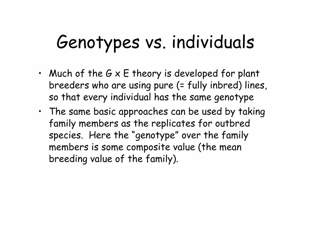
Genotypes vs. individuals
• Much of the G x E theory is developed for plantbreeders who are using pure (= fully inbred) lines,so that every individual has the same genotype
• The same basic approaches can be used by takingfamily members as the replicates for outbredspecies. Here the “genotype” over the familymembers is some composite value (the meanbreeding value of the family).
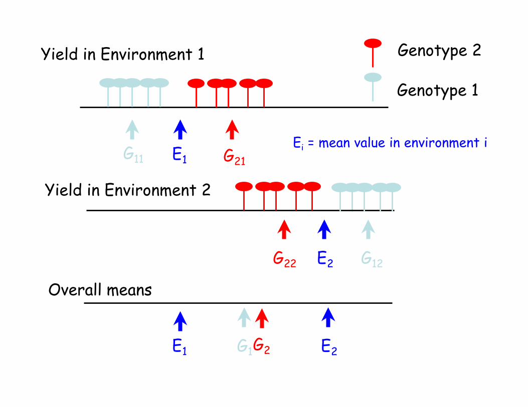
Yield in Environment 2
Yield in Environment 1
Genotype 1
Genotype 2
G11
G12
G21
G22
E1
E2
E2E1 G1 G2
Ei = mean value in environment i
Overall means
G11 G12G21 G22
E2E1 G1 G2
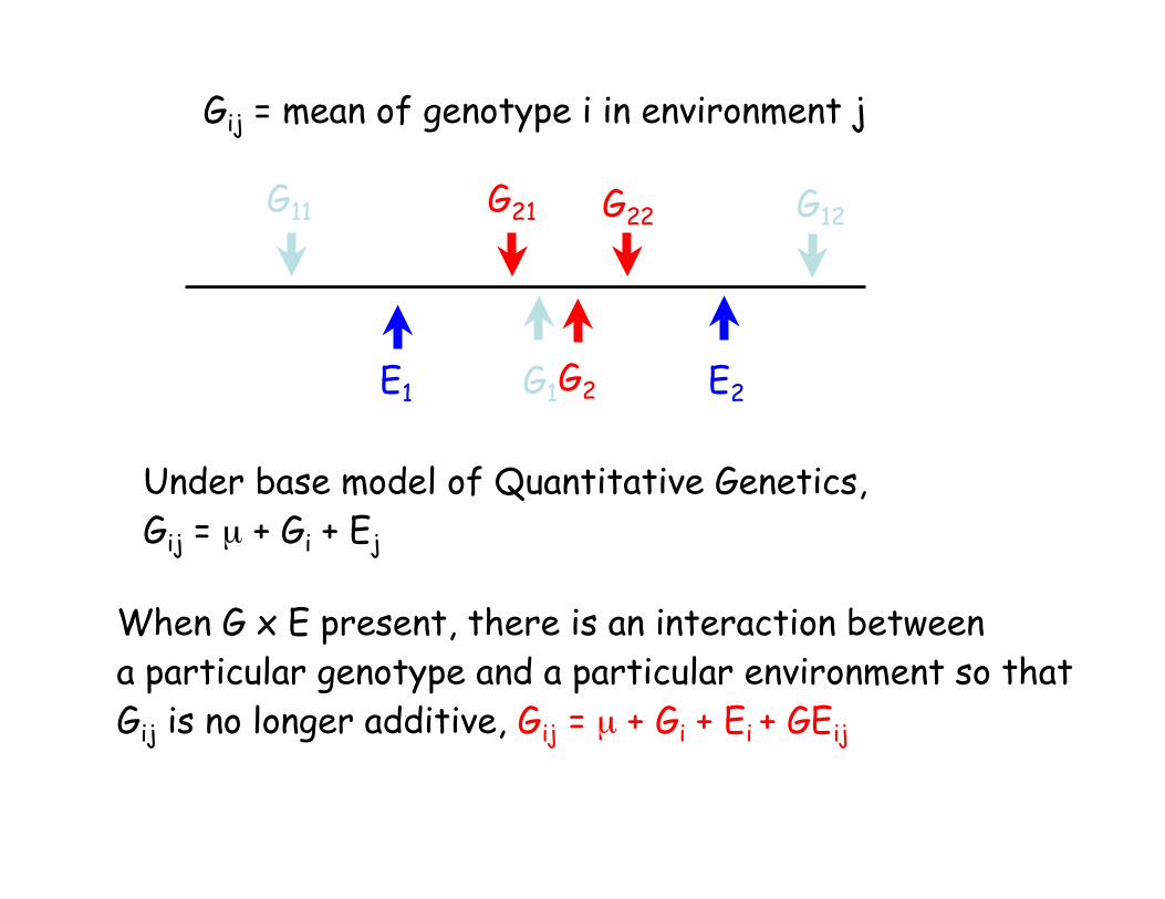
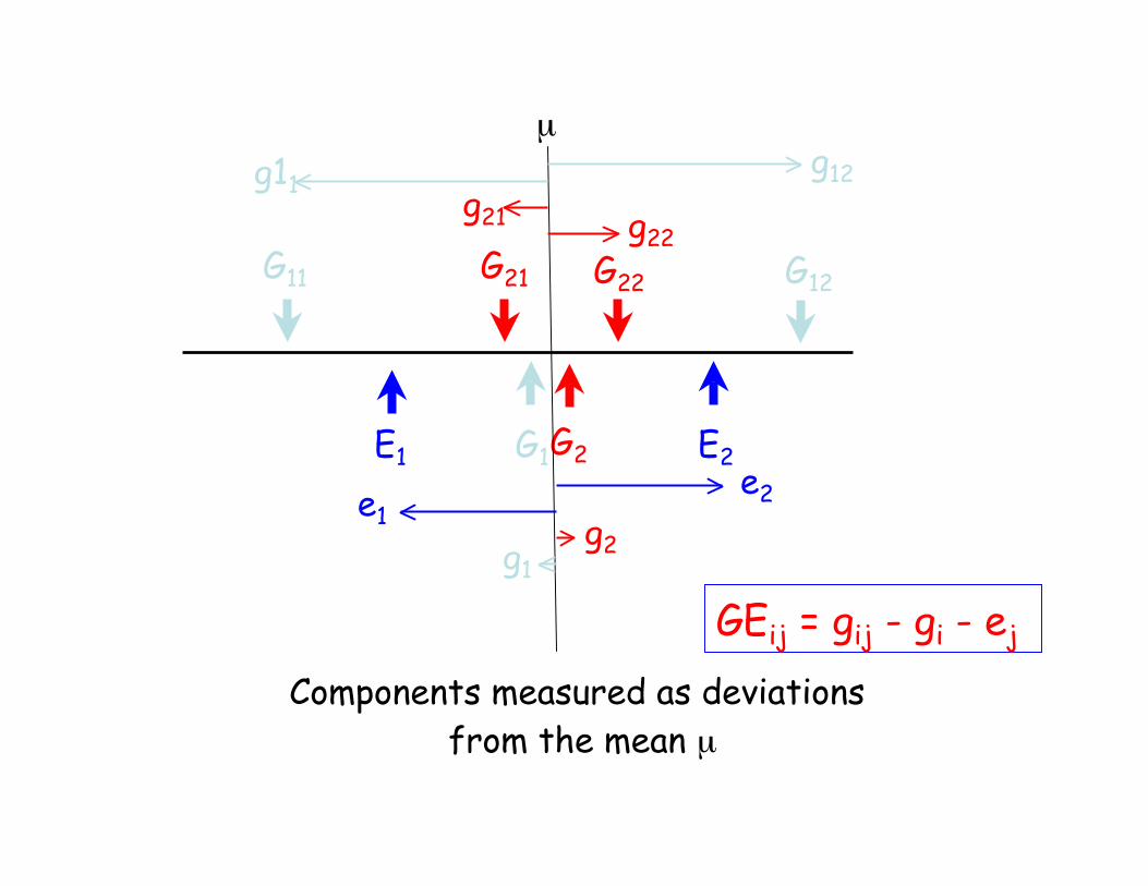
Gij = mean of genotype i in environment j
Under base model of Quantitative Genetics,
Gij = µ + Gi + Ej
When G x E present, there is an interaction between
a particular genotype and a particular environment so that
Gij is no longer additive, Gij = µ + Gi + Ei + GEij
G11 G12G21 G22
E2E1 G1 G2
µ
Components measured as deviations
from the mean µ
GEij = gij - gi - ej
e2e1
g1
g11g12
g2
g22g21
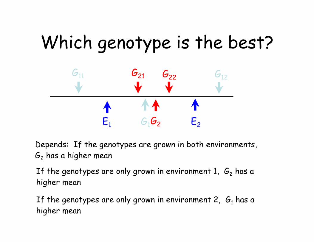
Which genotype is the best?
G11 G12G21 G22
E2E1 G1 G2
Depends: If the genotypes are grown in both environments,
G2 has a higher mean
If the genotypes are only grown in environment 1, G2 has a
higher mean
If the genotypes are only grown in environment 2, G1 has a
higher mean
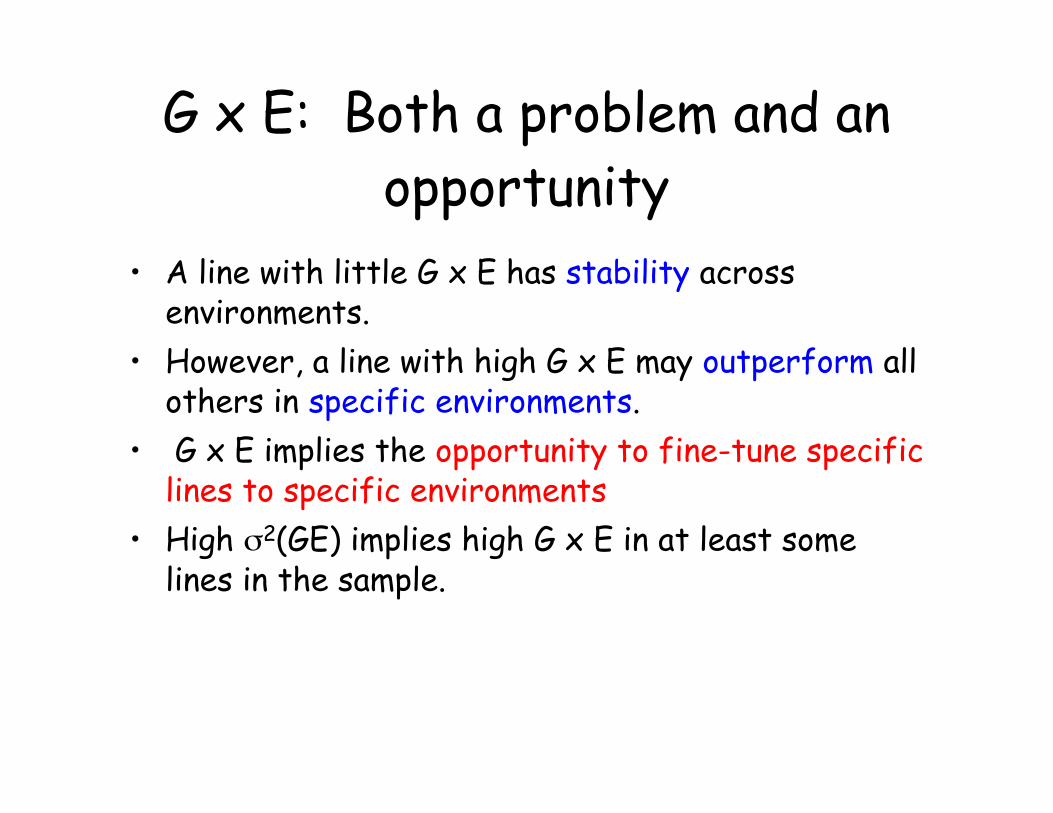
G x E: Both a problem and an
opportunity
• A line with little G x E has stability acrossenvironments.
• However, a line with high G x E may outperform allothers in specific environments.
• G x E implies the opportunity to fine-tune specificlines to specific environments
• High !2(GE) implies high G x E in at least somelines in the sample.
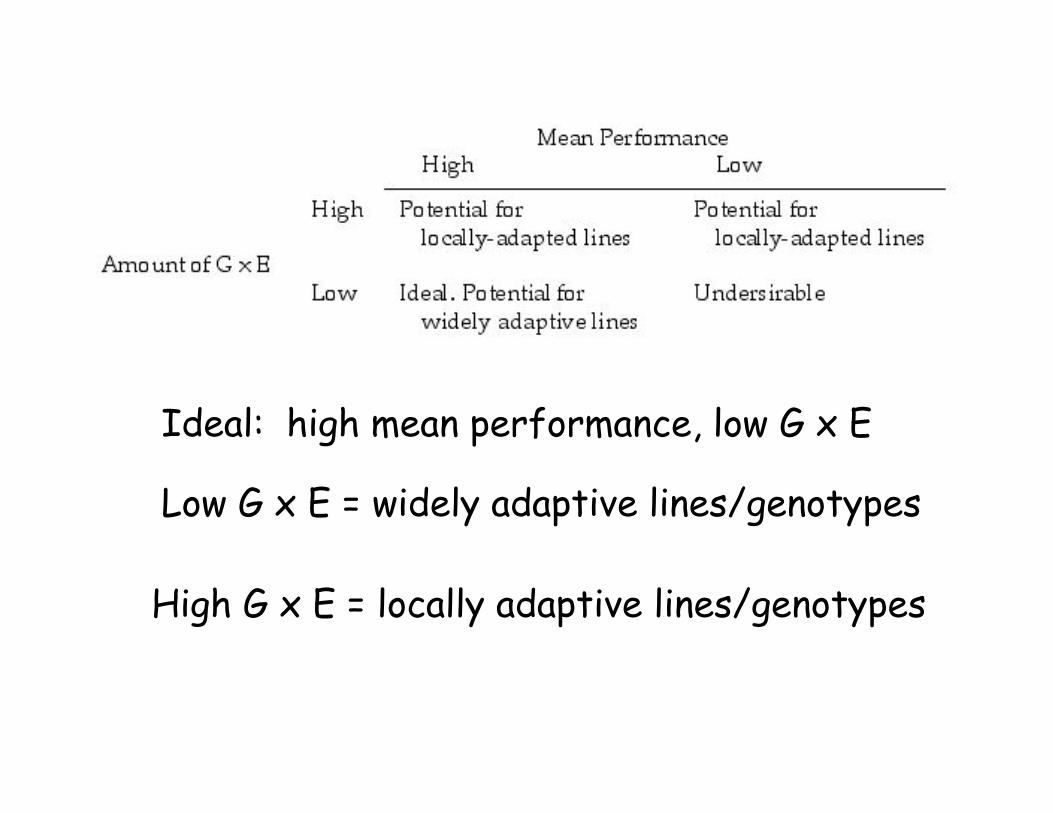
Ideal: high mean performance, low G x E
Low G x E = widely adaptive lines/genotypes
High G x E = locally adaptive lines/genotypes

Major vs. minor environments• An identical genotype will display slightly different traits
values even over apparently identical environments due tolow micro-environmental variation and developmental noise
• However, macro-environments (such as different locationsor different years <such as a wet vs. a dry year>) can showsubstantial variation, and genotypes (pure lines) maydifferentially perform over such macro-environments (G xE).
• Problem: The mean environment of a location may besomewhat predictable (e.g., corn in the tropics vs. temperateNorth American), but year-to-year variation at the samelocation is essentially unpredictable.
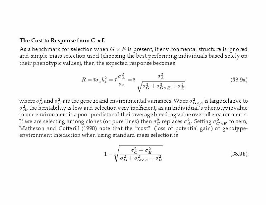
• Decompose G x E into components
– G x Elocations + G x Eyears + G x Eyears x locations
– Ideal: strong G x E over locations, high stability over years.

Key: differences in scale and lack of perfect correlation
over environments both generate G x E

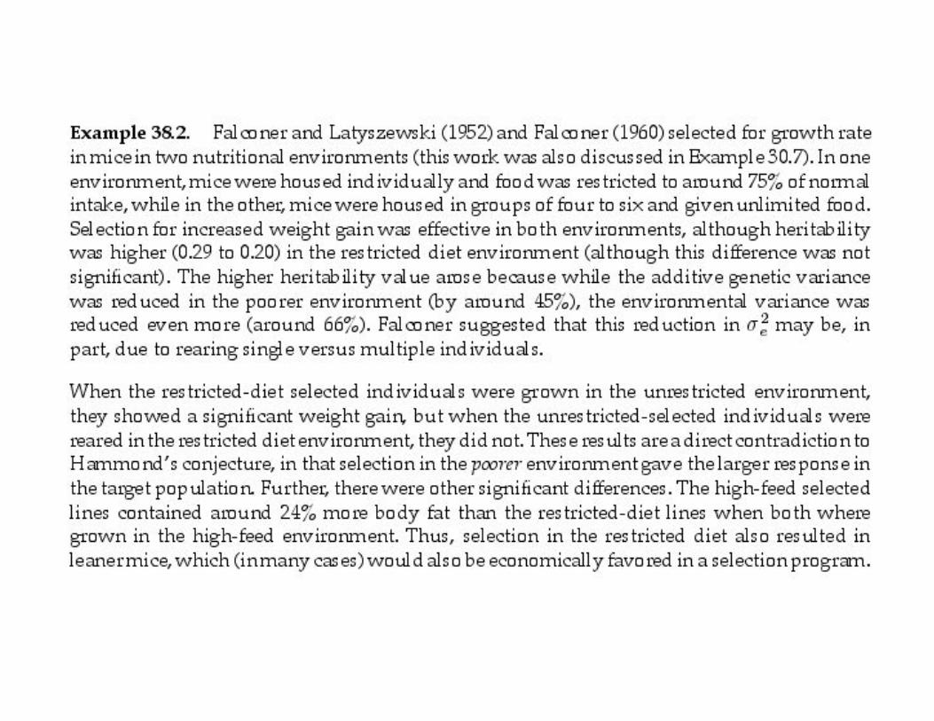
Falconer: G x E
• The modern treatment of G x E starts withFalconer (1952)– Measures of the same trait in different
environments are correlated traits
– Hence, if measured in k environments, it’s a k-dimensional trait
– Hence, results from direct and correlatedresponses apply to selection on G x E
• If selection in environment i, expectedchange in environment j is– CRj = ii hi hj rA !P (j)

Hammond’s Conjecture
• Hammond (1947) suggested that selectionbe undertaken in a more favorableenvironment to maximize progress in a lessfavorable one
• Idea: perhaps more genetic variation, andhence greater discrimination betweengenotypes
• Downside: don’t know if Var(G) greater in“better” environments, even if it is,between-environment correlation can besmall
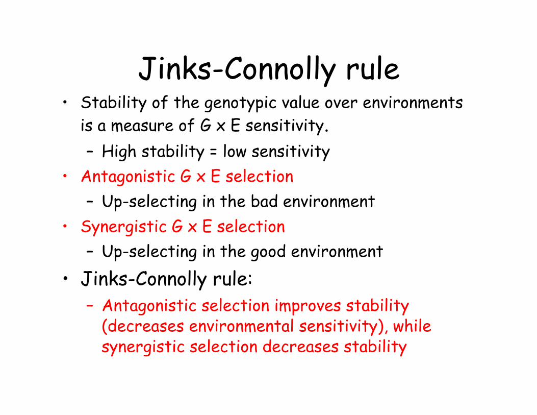
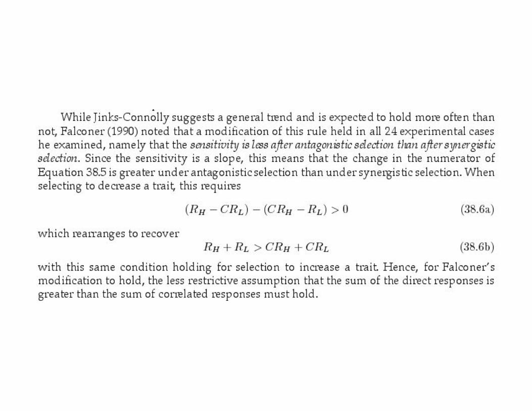
Jinks-Connolly rule• Stability of the genotypic value over environments
is a measure of G x E sensitivity.– High stability = low sensitivity
• Antagonistic G x E selection
– Up-selecting in the bad environment
• Synergistic G x E selection
– Up-selecting in the good environment
• Jinks-Connolly rule:– Antagonistic selection improves stability
(decreases environmental sensitivity), whilesynergistic selection decreases stability
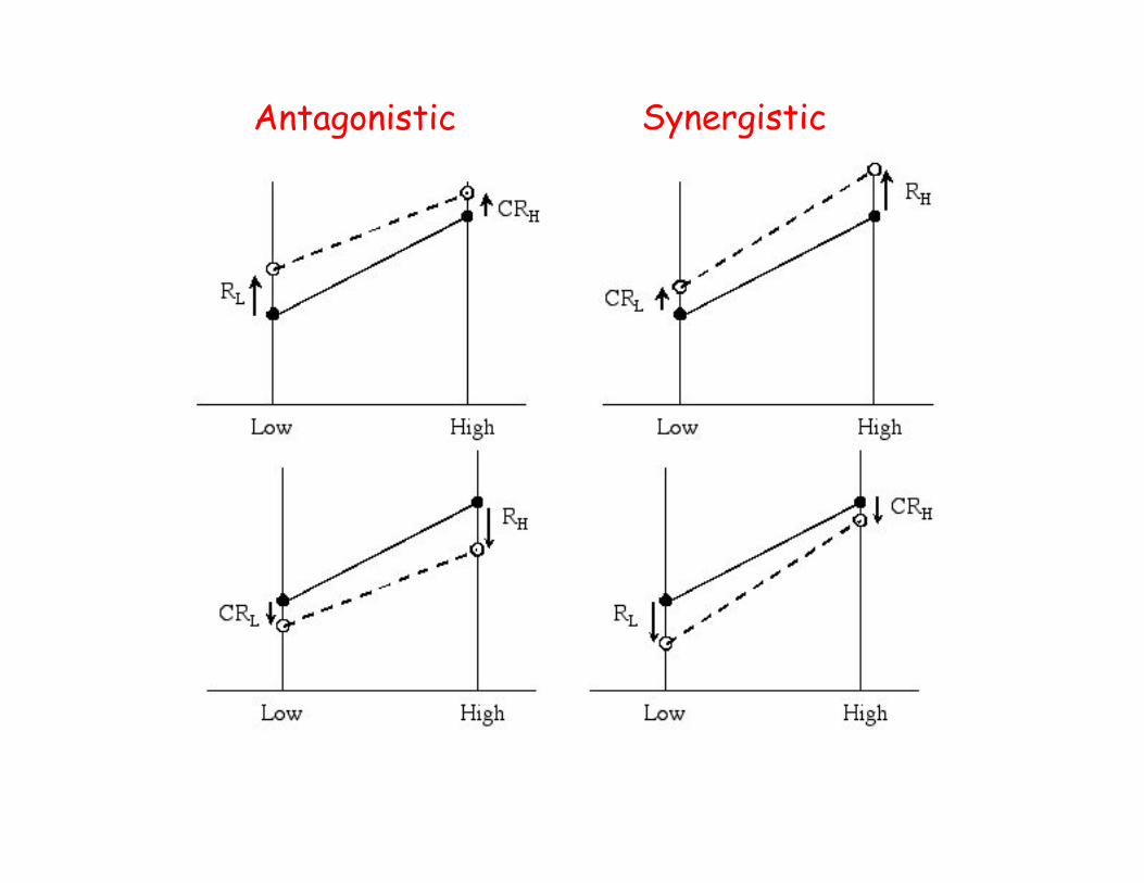
Antagonistic Synergistic
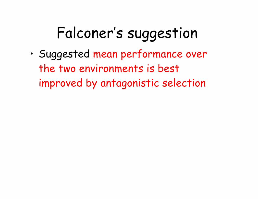
Falconer’s suggestion
• Suggested mean performance over
the two environments is best
improved by antagonistic selection


Replication over environments can reduce effect of
G x E in selection response
If members of the same genotype/line are replicated over ne
random environments, response to selection based on line
(or family) means is
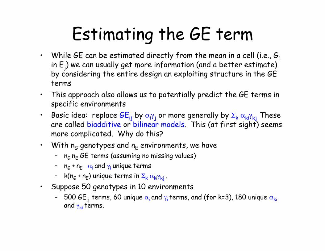
Estimating the GE term• While GE can be estimated directly from the mean in a cell (i.e., Gi
in Ej) we can usually get more information (and a better estimate)by considering the entire design an exploiting structure in the GEterms
• This approach also allows us to potentially predict the GE terms inspecific environments
• Basic idea: replace GEij by "i#j or more generally by $k "ki#kj Theseare called biadditive or bilinear models. This (at first sight) seemsmore complicated. Why do this?
• With nG genotypes and nE environments, we have
– nG nE GE terms (assuming no missing values)
– nG + nE "i and #i unique terms
– k(nG + nE) unique terms in $k "ki#kj .
• Suppose 50 genotypes in 10 environments
– 500 GEij terms, 60 unique "i and #i terms, and (for k=3), 180 unique "ki
and #ki terms.

Finlay-Wilkinson RegressionAlso called a joint regression or regression on an
environmental index.
Let µ + Gi be the mean of the ith genotype over all
the environments, and µ + Ej be the average yield of
all genotypes in environment j
The FW regression estimates GEij by the regression GEij = %iEj+ &ij.
The regression coefficient is obtained for each genotype from
the slope of the regression of the Gij over the Ej. &ij is the
residual (lack of fit). If !2(GE) >> !2(&) , then the regression
accounted for most of the variation in GE.

Application
• Yield in lines of wheat over differentenvironments was examined by Calderini andSlafer (1999). The lines they examined where linesfrom different eras of breeding (for fourdifferent countries)
• Newer lines had larger values, but also had higherslopes (large %i values), indicating less stabilityover mean environmental conditions than see inolder lines
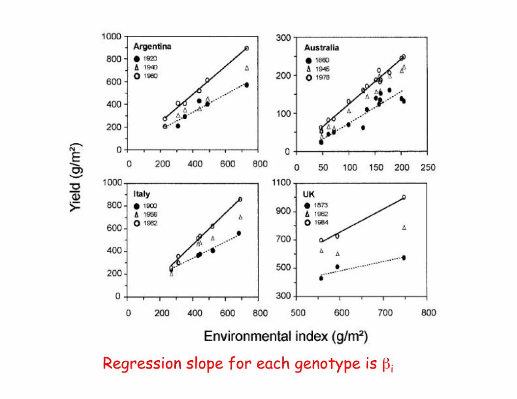
Regression slope for each genotype is %i
SVD approaches
• In Finlay-Wilkinson, the GEij term was estimatedby %iEj, where Ej was observed. We could alsohave used #jGi, where #j is the regression ofgenotype values over the j-th environment. AgainGi is observable.
• Singular-value decomposition (SVD) approachesconsider a more general approach, approximatingGEij by $k "ki#kj where the "ki and #kj aredetermined by the first k terms in the SVD of thematrix of GE terms.
• The SVD is a way to obtain the best approximationof a full matrix by some matrix of lower dimension


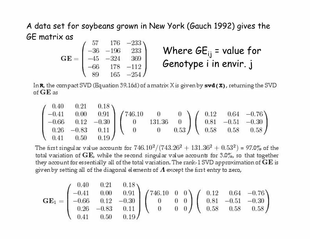
A data set for soybeans grown in New York (Gauch 1992) gives the
GE matrix as
Where GEij = value for
Genotype i in envir. j
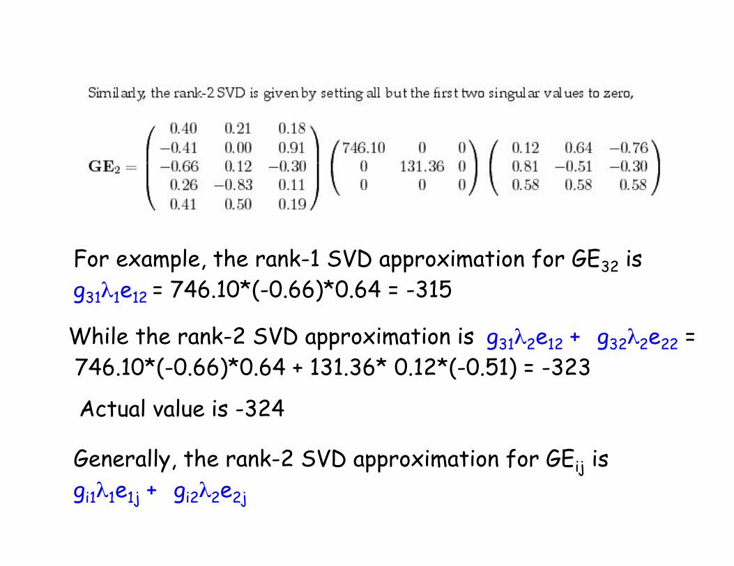
For example, the rank-1 SVD approximation for GE32 is
g31'1e12 = 746.10*(-0.66)*0.64 = -315
While the rank-2 SVD approximation is g31'2e12 + g32'2e22 =
746.10*(-0.66)*0.64 + 131.36* 0.12*(-0.51) = -323
Actual value is -324
Generally, the rank-2 SVD approximation for GEij is
gi1'1e1j + gi2'2e2j
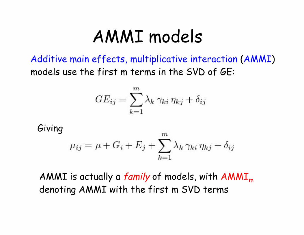
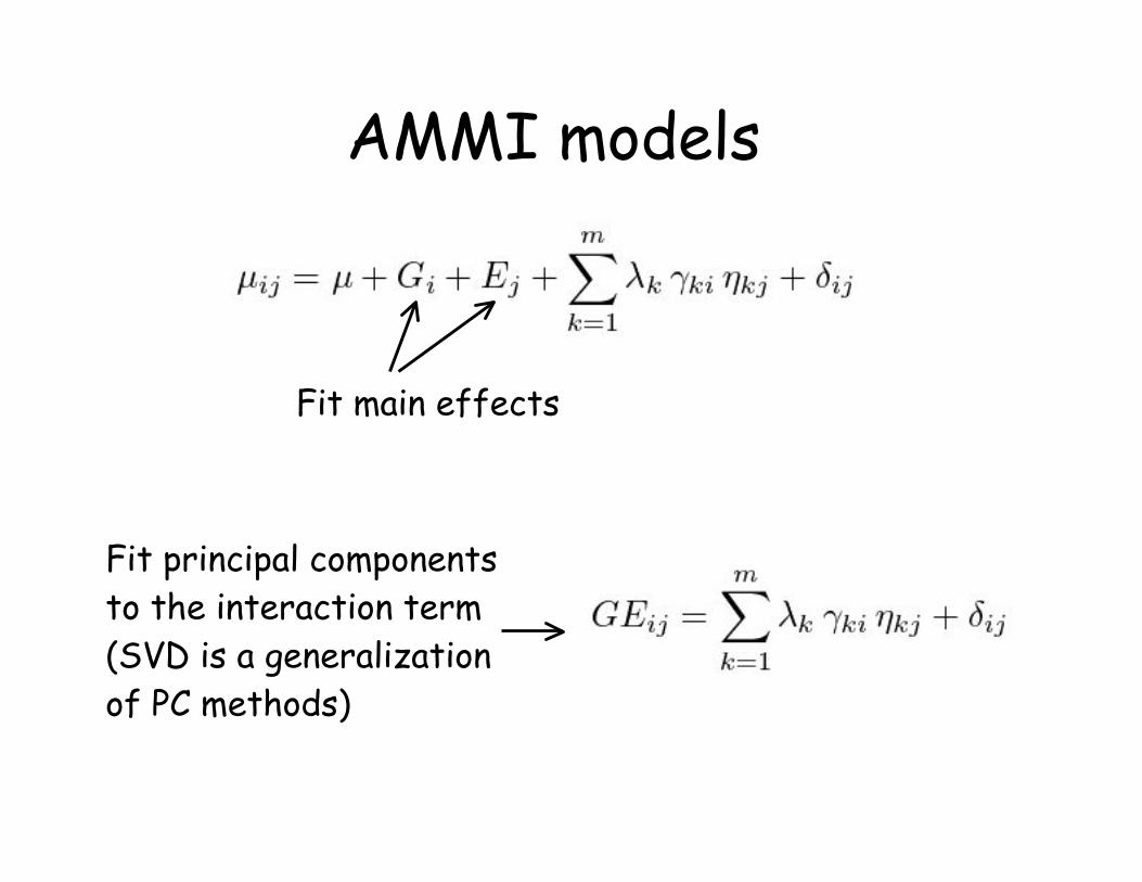
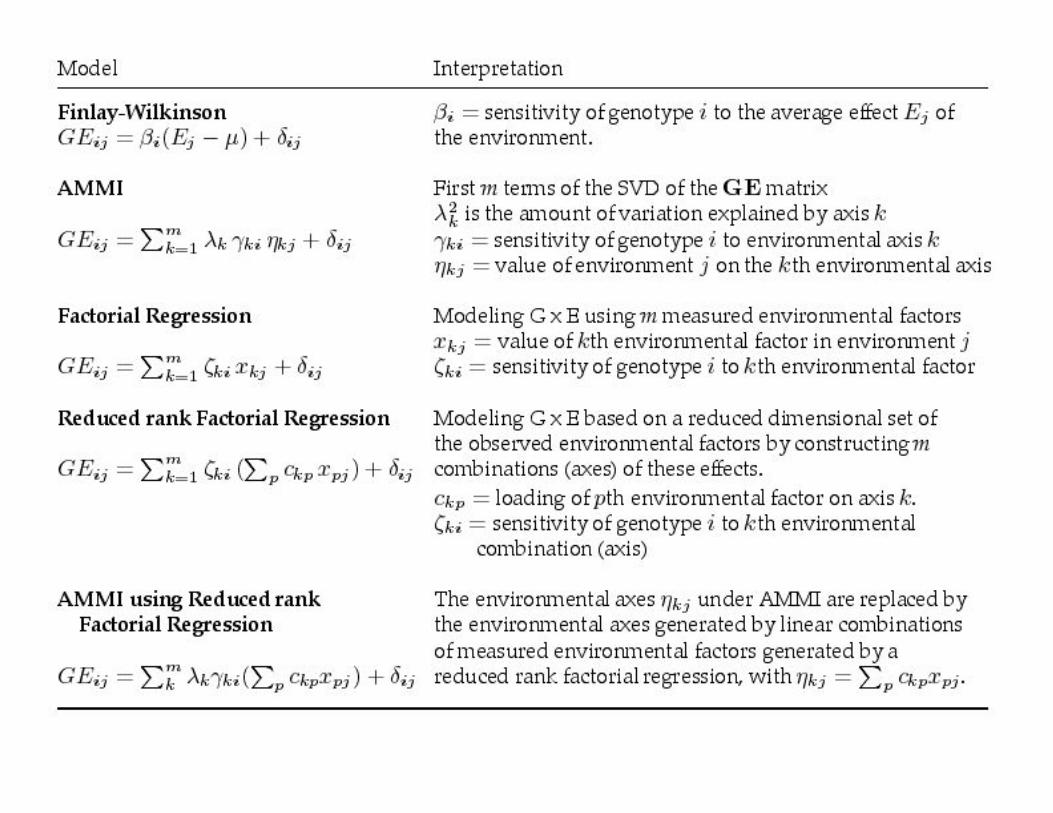
AMMI modelsAdditive main effects, multiplicative interaction (AMMI)
models use the first m terms in the SVD of GE:
Giving
AMMI is actually a family of models, with AMMIm
denoting AMMI with the first m SVD terms
AMMI models
Fit main effects
Fit principal components
to the interaction term
(SVD is a generalization
of PC methods)

Why do AMMI?
• One can plot the SVD terms (#ki, (kj) to visualizeinteractions– Called biplots (see Chapter 39 for details)
• AMMI can better predict mean values of GEij thanjust using the cell value (the observed mean ofGenotype i in Environment j)
• A huge amount more on AMMI in Chapter 33!

Factorial Regressions
• While AMMI models attempt to extract informationabout how G x E interactions are related across setsof genotypes and environments, factorial regressionsincorporate direct measures of environmentalfactors in an attempt to account for the observedpattern of G x E.
• The power of this approach is that if we candetermine which genotypes are more (or less)sensitive to which environmental features, thebreeder may be able to more finely tailor a line to aparticular environment without necessarily requiringtrials in the target environment.
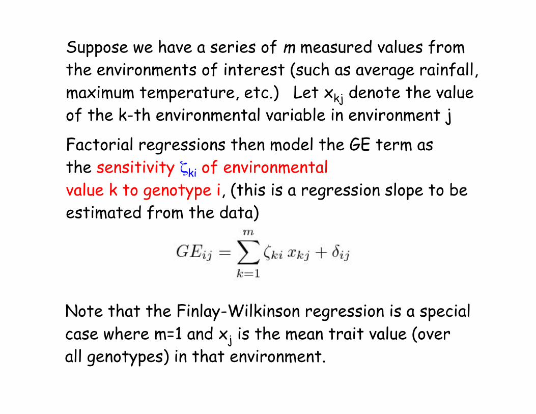
Suppose we have a series of m measured values from
the environments of interest (such as average rainfall,
maximum temperature, etc.) Let xkj denote the value
of the k-th environmental variable in environment j
Factorial regressions then model the GE term as
the sensitivity )ki of environmental
value k to genotype i, (this is a regression slope to be
estimated from the data)
Note that the Finlay-Wilkinson regression is a special
case where m=1 and xj is the mean trait value (over
all genotypes) in that environment.

Mixed model analysis of G x E• Thus far, our discussion of estimating GE has be set in terms of
fixed effects.
• Mixed models are a powerful alternative, as they easily handlemissing data (i.e., not all combinations of G and E explored).
• As with all mixed models, key is the assumed covariancestructure
– Structured covariance models
• Compound symmetry
• Finlay-Wilkinson
• Factor-analytic models (closely related to AMMI)
• Much more complete treatment and discussion in Chapter39

Basic GxE Mixed model• Typically, we assume either G or E is fixed, and
the other random (making GE random)
• Taking E as fixed, basic model becomes
• z = X% + Z1g + Z2ge + e– The vector % of fixed effects includes estimates of the Ej.
The vector g contains estimates of the Gi values, while thevector ge contains estimates of all the GEij.
– Typically we assume e ~ 0, !e2I, and independent of g and
ge.
– Models significantly differ on the variance/covariancestructure of g and ge.
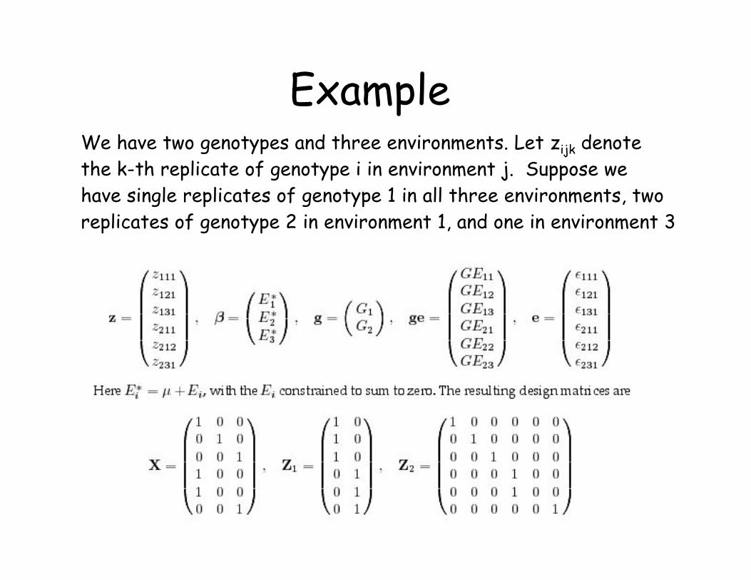
ExampleWe have two genotypes and three environments. Let zijk denote
the k-th replicate of genotype i in environment j. Suppose we
have single replicates of genotype 1 in all three environments, two
replicates of genotype 2 in environment 1, and one in environment 3
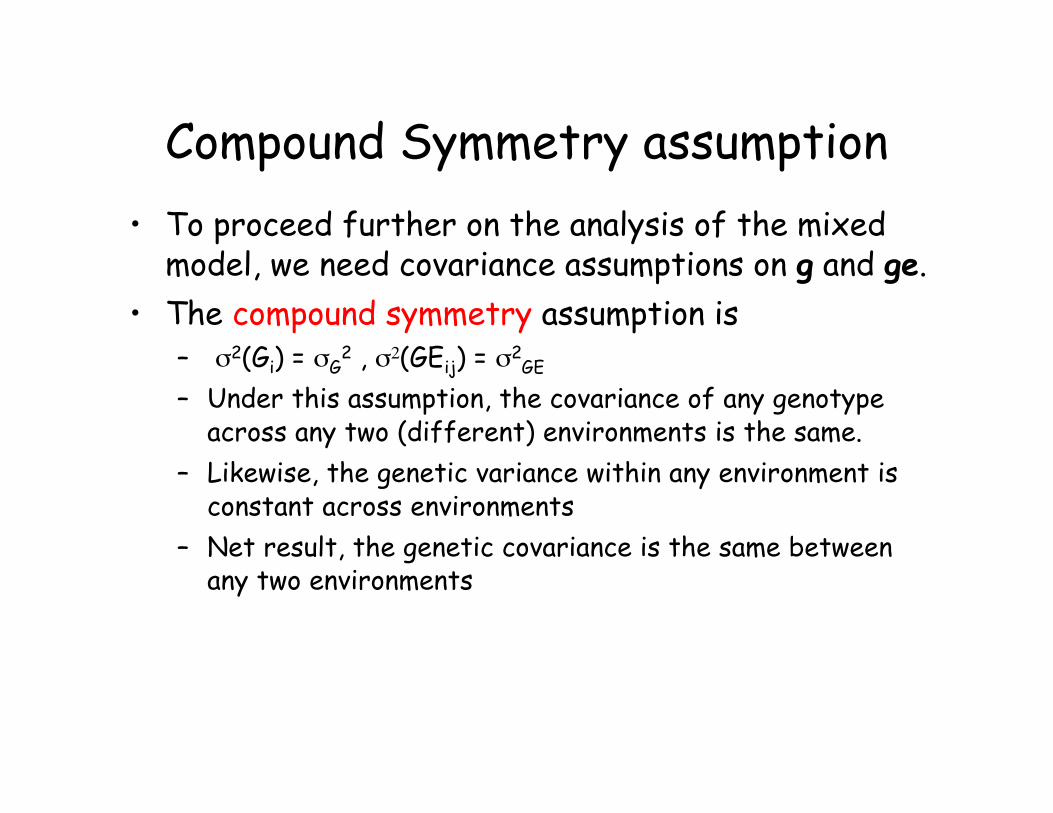
Compound Symmetry assumption
• To proceed further on the analysis of the mixedmodel, we need covariance assumptions on g and ge.
• The compound symmetry assumption is– !2(Gi) = !G
2 , !2(GEij) = !2GE
– Under this assumption, the covariance of any genotypeacross any two (different) environments is the same.
– Likewise, the genetic variance within any environment isconstant across environments
– Net result, the genetic covariance is the same betweenany two environments
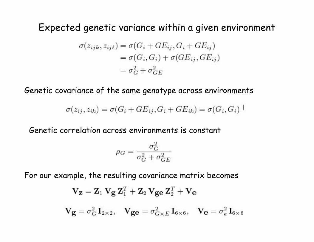
Expected genetic variance within a given environment
Genetic correlation across environments is constant
Genetic covariance of the same genotype across environments
For our example, the resulting covariance matrix becomes

Mixed-model allows for missing values.
Under fixed-model model, estimate of µij = zij.
BLUP estimates under mixed-model (E fixed, G random)
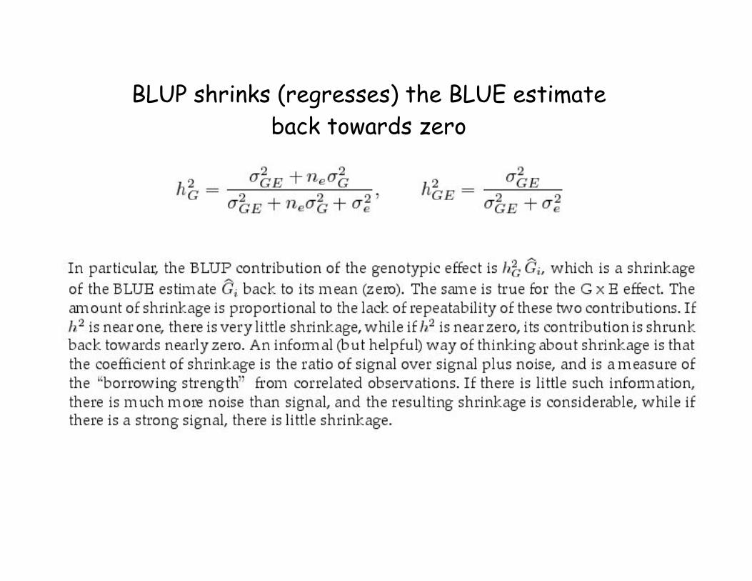
BLUP shrinks (regresses) the BLUE estimate
back towards zero

Modification of the residual
covariance
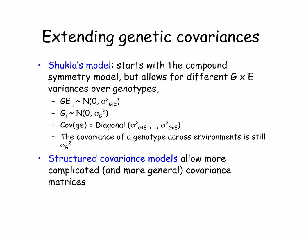
Extending genetic covariances
• Shukla’s model: starts with the compoundsymmetry model, but allows for different G x Evariances over genotypes,– GEij ~ N(0, !2
GiE)
– Gi ~ N(0, !G2)
– Cov(ge) = Diagonal (!2G1E ,
…, !2GnE)
– The covariance of a genotype across environments is still!G
2
• Structured covariance models allow morecomplicated (and more general) covariancematrices
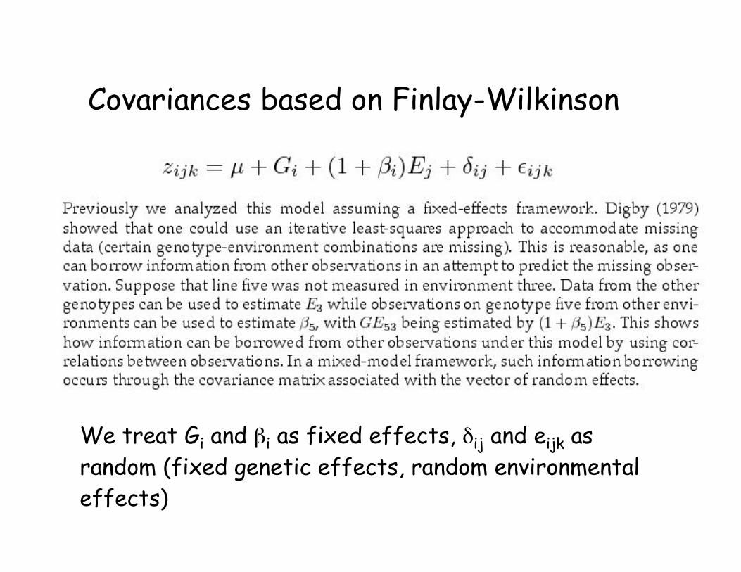
Covariances based on Finlay-Wilkinson
We treat Gi and %i as fixed effects, &ij and eijk as
random (fixed genetic effects, random environmental
effects)
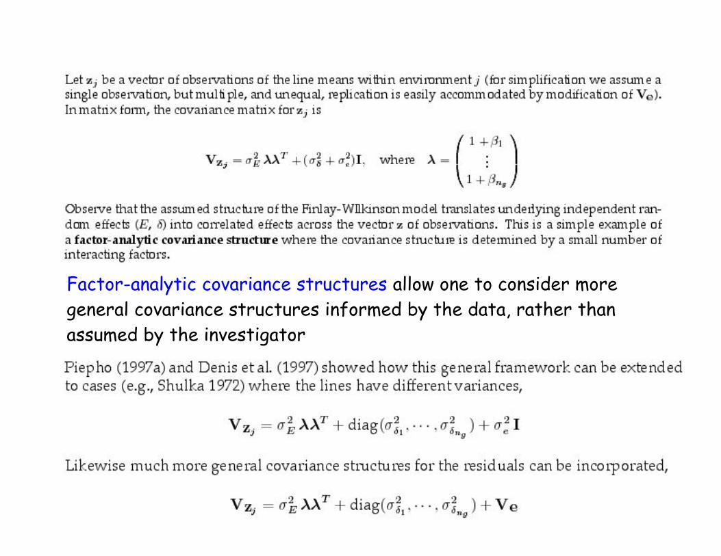
Factor-analytic covariance structures allow one to consider more
general covariance structures informed by the data, rather than
assumed by the investigator
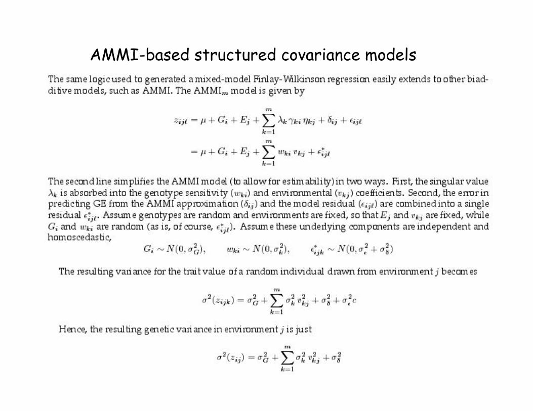
AMMI-based structured covariance models

Chapter 39 goes into detail on further analysis of this
model, and its connection to stability analysis and the
response to selection.

Summary: Structured Covariance models