GAME THEORY APPROACH TO THE VERTICAL RELATIONSHIPS FOR U.S.

CONTAINERIZED IMPORTS

A Dissertation Submitted to the Graduate Faculty

of the North Dakota State University

of Agriculture and Applied Science

By

Qing Liu

In Partial Fulfillment for the Degree of

DOCTOR OF PHILOSOPHY

Major Program: Transportation and Logistics

Option: Transportation Economics

October 2013

Fargo, North Dakota

North Dakota State University Graduate School

Title

Game Theory Approach to the Vertical Relationships for U.S. Containerized Imports

By

Qing Liu

The Supervisory Committee certifies that this disquisition complies with North Dakota State

University’s regulations and meets the accepted standards for the degree of

DOCTOR OF PHILOSOPHY

SUPERVISORY COMMITTEE: Dr. William Wilson

Chair

Dr. Denver Tolliver

Dr. Joseph Szmerekovsky

Dr. Gang Shen

Approved: November 12, 2013 Dr. William Wilson Date Department Chair

ABSTRACT

Multi-player interactions and vertical relationships in the U.S. containerized-import

shipment market are investigated using game theory approaches. Bi-level programming

problems (BLPP) are built to capture the hierarchy structure of the container shipping industry,

whereas the ocean carriers (OC) are considered as the market leader. For a case study with five

players from several levels of the shipment chain, 16 BLPPs are built to analyze the 32 coalition

possibilities. Two routes are compared: The West Coast route (WCR) includes one terminal (P1)

and one railroad (R); the East Coast route (ECR) includes a second terminal (P2) and the Panama

Canal (PC). The impact of Panama Canal expansion is investigated by comparing scenarios with

different assumptions of vessel size. Capacity constraints at port terminals are also analyzed by

assuming different capacity levels.

The grand coalition of the five players is found to be very unstable because of the

unavoidable competition within the coalition; hence, following games are further created,

supposing the grand coalition could not form. Model results indicate the OC prefers to form an

East Coast Coalition (ECC) with East Coast players if the grand coalition could not form.

Sensitivity analyses on some parameter values for the grand coalition and for the ECC

bring some interesting findings. With higher cargo values, the WCR becomes more appealing

because of its quicker delivery time and lower inventory costs compared with the ECR. The

Panama Canal expansion will improve market power and profit shares for the East Coast players

if the canal operator could increase its competitive price more than the increase of costs.

Generally, a player will gain more market power if its cost could be reduced. A player’s upper

bound rate is a reflection of its relative market power. But in a complicated market characterized

iii

with various cooperation-competition strategies and an ambiguous definition of partners and

competitors, the impact of a player’s upper bound rate on the market power structure could not

be easily explained. For future research, the challenge mainly lies on the large number of BLPPs

that need to be constructed and solved in order to study more players.

iv

ACKNOWLEDGEMENTS

The last few years have been an unforgettable experience. I would never be able to finish

my dissertation without the support from all my friends and help from all my committee

members.

I would like to thank my advisor, Dr. Wilson, for inspiring me toward the research idea,

and for his knowledgeable guidance through the whole process. I am thankful for his trust and

continuous availability when I had to move to West Virginia for my new job. I also would

express my sincere gratitude to Dr. Tolliver, Dr. Szmerekovsky, and Dr. Shen for serving on my

committee board and offering me their solid knowledge in their different expertise fields.

I sincerely appreciate everything I received from the Transportation and Logistics

program at North Dakota State University. All the staff and colleagues have been so friendly and

helpful that I could enjoy a fruitful and memorable Ph.D. education. The program director, Dr.

Tolliver, has been my supervisor for most of those years and has also been a great friend. His

encouragement, trust, and professional guidance have never stopped for me.

I am also deeply grateful to my current employer, Rahall Transportation Institute, for

encouraging me to work toward my degree during the year. I have met many excellent

professionals and great friends. Their trust and friendship are priceless.

My deepest gratitude goes to my family, especially my parents, who raised me up and

stood by me through my life. I greatly appreciate the sacrifice they made to help me take care of

my two-year-old son, Endi, during the past year. It has been a tremendous help. And thank you,

Endi, for being my sweetest boy and my great comfort.

There is no way I could fully express my gratitude and list everyone that has helped me. I

just want to say: Thank you, all my friends.

v

TABLE OF CONTENTS

ABSTRACT ................................................................................................................................... iii

ACKNOWLEDGEMENTS .............................................................................................................v

LIST OF TABLES ...........................................................................................................................x

LIST OF FIGURES ...................................................................................................................... xii

LIST OF APPENDIX TABLES .................................................................................................. xiv

1. INTRODUCTION .................................................................................................................. 1

1.1. Background ...................................................................................................................... 1

1.1.1. Uncertainties in the World Container Shipping Market ........................................... 1

1.1.2. Market Structure of the Ocean Container-Shipping Industry ................................... 3

1.1.3. Inter-Port Competition .............................................................................................. 5

1.1.4. Vertical Integration of the Shipment Chain .............................................................. 6

1.1.5. Relationships Between Shipping Companies and Other Players .............................. 7

1.1.6. Shipment Chain Structures ....................................................................................... 8

1.2. Problem Statement and Research Objectives ................................................................. 11

1.3. Organization of the Dissertation .................................................................................... 13

2. LITERATURE REVIEW OF GAME THEORY APPLICATIONS .................................... 15

2.1. Optimization Modeling for Containerized Cargo Flows................................................ 15

vi

2.2. Freight Network Equilibrium Model and Spatial Price Equilibrium Model .................. 17

2.3. Game Theory Application in Ocean Shipping Industry ................................................. 19

2.4. Game Theory Application in Transportation ................................................................. 21

2.5. Application of Cooperative Game Theory to Supply Chain Management .................... 25

2.6. Conclusions of Literature Review .................................................................................. 27

3. METHODOLOGY ............................................................................................................... 29

3.1. Preliminaries of Cooperative Game Theory................................................................... 29

3.1.1. Introduction of CGT ............................................................................................... 29

3.1.2. The Core.................................................................................................................. 31

3.1.3. The Shapley Value .................................................................................................. 32

3.1.4. Least Core and Minmax Core ................................................................................. 35

3.2. Stackelberg Game and Bi-Level Programming Problem ............................................... 36

3.2.1. Stackelberg Game and Hierarchy Decision Making by BLPP ............................... 36

3.2.2. Solution of BLPP .................................................................................................... 37

4. MODEL CONSTRUCTION ................................................................................................ 42

4.1. Bi-Level Model Formulations and Cooperation Schemes ............................................. 43

4.2. Basic Model Components .............................................................................................. 44

4.2.1. Notation Set ............................................................................................................ 45

4.2.2. List of Functions ..................................................................................................... 46

4.3. Illustration of Example Models ...................................................................................... 47

vii

4.3.1. Model Example 2 .................................................................................................... 48

4.4. KKT Transformation of the Bi-Level Model ................................................................. 49

4.4.1. Original Model Example Model 2 .......................................................................... 49

4.4.2. Transfer the Second level by KKT ......................................................................... 49

5. CASE STUDY ...................................................................................................................... 50

5.1. Coalitions and Models .................................................................................................... 50

5.1.1. Model 1 Illustration................................................................................................. 51

5.1.2. Model Solution and Shapley Value Calculation ..................................................... 53

5.2. Parameter Estimates ....................................................................................................... 55

5.2.1. Daily Vessel Operating Cost ................................................................................... 55

5.2.2. Transit Time Estimates ........................................................................................... 58

5.2.3. Inventory Cost ......................................................................................................... 60

5.2.4. Transportation Rates ............................................................................................... 62

6. RESULT ANALYSIS ........................................................................................................... 66

6.1. Model Results and CGT Solutions ................................................................................. 66

6.2. Result Interpretation ....................................................................................................... 74

6.3. Sensitivity Analysis ........................................................................................................ 78

6.3.1. Impacts of Cargo Values ......................................................................................... 79

6.3.2. Impacts of Charging Rates ...................................................................................... 80

6.3.3. Impacts of Capacity Constraint Assumption .......................................................... 84

viii

6.4. Conclusions of Case Study ............................................................................................. 85

7. FOLLOWING GAMES ........................................................................................................ 88

7.1. West Coast Coalition and East Coast Coalition ............................................................. 88

7.2. Sensitivity Analysis for the Following Games ............................................................... 93

7.3. Conclusions of Following Games .................................................................................. 96

8. SUMMARY AND CONCLUSIONS ................................................................................... 99

8.1. Summary of the Problem................................................................................................ 99

8.2. Summary of Model Results .......................................................................................... 100

8.3. Implications .................................................................................................................. 101

8.4. Contributions ................................................................................................................ 102

8.5. Limitations, Challenges and Suggestions for Future Research .................................... 103

REFERENCES ........................................................................................................................... 106

APPENDIX A. LIST OF MODELS AND CONSTRAINTS ..................................................... 116

APPENDIX B. MODEL RESULTS........................................................................................... 119

APPENDIX C. FOLLOWING GAME RESULTS .................................................................... 121

ix

LIST OF TABLES

Table Page

5.1. Fuel Consumption Rates and Economic Speeds of the Vessels .............................................56

5.2. Vessel Time Estimates ............................................................................................................59

5.3. Container Inland Time Estimates for WCR ............................................................................60

5.4. Daily Pipeline Inventory Cost Calculation .............................................................................62

5.5. Railway Shipment Rates Summary ........................................................................................64

6.1. Shapley Values and Value Ratios in S1, S2, S3, S4 ...............................................................67

6.2. Unit Profit Values in S1, S2, S3, S4 .......................................................................................67

6.3. Coalition Values for S1 ...........................................................................................................68

6.4. Coalition Values for S2 ...........................................................................................................69

6.5. Coalition Values for S3 ...........................................................................................................70

6.6. Coalition Values for S4 ...........................................................................................................71

6.7. Least Core for S1, S2, S3 and S4 ............................................................................................72

6.8. Minmax Core for S1, S2, S3 and S4 .......................................................................................72

7.1. Shapley Values and Value Ratios for West Coast Coalition {OC, P1, R} .............................88

7.2. Shapley Values and Value Ratios for East Coast Coalition {OC, P2, PC} ............................88

7.3. West Coast Coalition Values in S1 .........................................................................................89

7.4. West Coast Coalition Values in S2 .........................................................................................89

7.5. East Coast Coalition Values in S1 ..........................................................................................89

7.6. East Coast Coalition Values in S2 ..........................................................................................90

7.7. Shapley Value Changes Due to Cooperation of ECC in S1 ...................................................90

7.8. Least Core for ECC in S1 .......................................................................................................92

x

7.9. Minmax Core for ECC in S1 ..................................................................................................92

7.10. Shapley Value Changes with PC Lower Bound Rate in S1..................................................93

7.11. Shapley Value Changes with P2 Lower Bound Rate in S1 ..................................................94

7.12. Shapley Value and Ratio Changes with PC Upper Bound Rate in S1 ..................................94

7.13. Shapley Value and Ratio Changes with P2 Upper Bound Rate in S1 ..................................95

7.14. Shapley Value and Ratio Changes with CRL and CRU in S2 ..............................................96

7.15. Shapley Value and Ratio Changes with PRL and PRU in S2 ...............................................96

xi

LIST OF FIGURES

Figure Page

1.1. Decision Flow and Product Flow in a Supply Chain ..............................................................10

1.2. Decision Flow and Freight Flow in a Container Shipment Chain ..........................................10

5.1. HVO and MDO Price Changes ...............................................................................................57

5.2. Daily Hire Rates Changes .......................................................................................................57

5.3. Daily Hire Rates Estimation ...................................................................................................58

6.1. Comparisons of Shapley Value, LC, MMC for S1 .................................................................72

6.2. Comparisons of Shapley Value, LC, MMC for S2 .................................................................73

6.3. Comparisons of Shapley Value, LC, MMC for S3 .................................................................73

6.4. Comparisons of Shapley Value, LC, MMC for S4 .................................................................74

6.5. Panama Canal Expansion Impact S1 vs. S2............................................................................75

6.6. Panama Canal Expansion Impact S3 vs. S4............................................................................76

6.7. Terminal Capacity Constraint Impact S1 vs. S3 .....................................................................77

6.8. Terminal Capacity Constraint Impact S2 vs. S4 .....................................................................77

6.9. Shapley Value Changes with Cargo Values in S1 ..................................................................79

6.10. Shapley Value Ratio Changes with Cargo Values in S1 ......................................................80

6.11. Shapley Value Changes with Railroad Rate Lower Bound in S1 .........................................81

6.12. Shapley Value Ratios Changes with Railroad Rate Lower Bound in S1 .............................81

6.13. Shapley Value Changes with Railroad Rate Upper Bound in S1 .........................................81

6.14. Shapley Value Ratio Changes with Railroad Rate Upper Bound in S1 ...............................82

6.15. Shapley Value Changes with Panama Canal Rate Lower Bound in S1 ...............................82

6.16. Shapley Value Ratio Changes with Panama Canal Rate Lower Bound in S1 ......................83

xii

6.17. Shapley Value Changes with Panama Canal Rate Upper Bound in S1 ................................83

6.18. Shapley Value Ratio Changes with Panama Canal Rate Upper Bound in S1 ......................84

6.19. Shapley Value Changes with OC Rates in S1 ......................................................................84

6.20. Shapley Value Changes with Terminal Capacity Constraints ..............................................85

6.21. Shapley Value Ratio Changes with Terminal Capacity Constraints ....................................85

7.1. Comparisons of Shapley Value, LC, MMC for ECC in S1 ....................................................92

7.2. Comparisons of Shapley Value, LC, MMC for ECC in S2 ....................................................93

xiii

LIST OF APPENDIX TABLES

Table Page

A.1. Model List for Case Study ...................................................................................................116

A.2. Constraint Sets .....................................................................................................................117 B.1. S1 Results .............................................................................................................................119

B.2. S2 Results .............................................................................................................................119

B.3. S3 Results .............................................................................................................................120

B.4. S4 Results .............................................................................................................................120 C.1. Model Results for {OC, P1, R} in S1 ..................................................................................121

C.2. Model Results for {OC, P1, R} in S2 ..................................................................................121

C.3. Model Results for {OC, P2, PC} in S1 ................................................................................121

C.4. Model Results for {OC, P2, PC} in S2 ................................................................................121

C.5. Model Results for {OC, P2, PC} with No Cooperating Benefit in S1 .................................121

xiv

1. INTRODUCTION

The economic background for this dissertation is briefly discussed first, including the

container-shipping market problems, market structures, port competition, and relationships

among players along the container shipment chains. Research problems and objectives are

introduced in the second section. The organization of the whole dissertation is given in the end.

1.1. Background

1.1.1. Uncertainties in the World Container Shipping Market

There are many issues confronting the container shipping industry: uncertainty in the

world economy and international trade, over-capacity caused by orders placed before the

economic crisis, fierce competition within the industry (or from outside), etc. Overall, the global

container market has been growing fast. Since 2005, the containership fleet has nearly tripled.

The world merchant fleet reached almost 1.4 billion deadweight tons (DWT) in January 2011, an

increase of 120 million DWT over 2010. New deliveries stood at 150 million DWT, despite

approximately 30 million DWT of demolitions and other withdrawals from the market. The

surge in the capacity supply makes the competition even harder than it was previously

(UNCTAD 2011).

Developments in world seaborne trade and the shipping industry mirrored the

performance of the broad world economy. Seaborne trade is subject to the same uncertainties and

shocks that may undermine the prospects of a sustained recovery. From 1995 to 2009, the

continuing expansion on three major East-West container routes was compelling, followed by a

drastic drop in 2009 because of the 2008 world economy downturn. Container carriers decreased

their production levels and scrapped old equipment, including ships and container boxes, to cut

1

costs. With the world economic situation brightening in 2010, the seaborne trade volumes

recorded a positive turnaround, especially in the dry bulk and container trade segments. In 2010,

global container trade volumes bounced back at 12.9% over the 2009 level with a demand surge

for almost all trade lanes, which were among the strongest growth rates in the history of

containerization. With trade growing at an unexpectedly fast rate, a capacity shortage was

observed in the fourth quarter of 2009 and early 2010 (UNCTAD 2011).

Another major uncertainty for U.S. containerized import distribution is the Panama Canal

expansion. Currently, the maximum capacity of a ship that could cross the Panama Canal (a

Panamax ship) is 4,800 Twenty-foot Equivalent Units (TEU). By the end of 2014, the Panama

Canal is scheduled to have completed its greatest expansion, allowing it to handle some of the

world’s most massive ships. Much bigger ships will be allowed: 50% wider, 25% longer, and a

volume of more than 12,000 TEUs. The Panama Canal expansion will have deep, but uncertain,

impacts on U.S. ports as well as the U.S. container import and export flow distributions. Many

expect a positive impact on the East and Gulf Coast ports, with a slightly negative impact on the

West Coast ports because more Asian container ships would divert to the other side of the United

States. Many factors may affect the changes. For example, to accommodate bigger ships, state

governments and their port authorities along the Gulf and East Coasts are seeking to spend

billions of dollars dredging their harbors and increasing the minimum depth from 39.5 feet to 50

feet as quickly as possible. However, U.S. harbor-dredging projects need federal approval and

funding, which is an enormously complicated process. On the other hand, there are some

observers who do not necessarily agree that the Panama Canal expansion will have major effects

on the United States. In a 2010 report, the southern office of the Council of State Governments

noted that one school of thought contends that East Coast ports are already struggling to handle

2

loads from smaller ships and would not be able to manage bigger ships even if the ports were

technically deep enough. Others doubt that shipping routes would change that drastically because

many shippers would still place a premium on speed. Nevertheless, most people still believe the

forecast based on the Panama Canal expansion; even if it does not play out in the short term, it

definitely will over time (Holeywell 2012).

1.1.2. Market Structure of the Ocean Container-Shipping Industry

Because of the container shipping industry’s instability and fierce competition, ship

owners and carriers have been making various efforts to minimize the risk and better manage

their operations, such as varying the cruising speeds at sea and increasing vessel sizes. During a

time of compressed demand, for example, slow steaming could be implemented to cut fuel costs

and absorb capacity. A larger vessel size is a classic approach to enhance fuel efficiency, reduce

average operating cost, and gain higher market power. Market power is concerned with the

ability of firms to secure stronger positions in their market as a means of achieving competitive

advantage. Shepherd (1970) defined market power as “the ability of a market participant or

group of participants to influence price, quality, and the nature of the product in the market

place.”

However, for many shipping companies, these individual approaches are not enough for

survival; various forms of cooperation agreements, including strategic alliances, mergers, and

acquisitions, emerged as the most effective method for this industry. The first cooperative

agreement formed by ocean shipping companies was established in the 1870s in an effort to

eliminate fierce competition by limiting capacity and fixing freight rates. By 2011, almost all

global carriers had been involved in some kinds of global alliances, except for the biggest

companies which have a large fleet and a wide service network, such as the Mediterranean

3

Shipping Company and Maersk Line. Inside the strategic global alliances, various types of

collaborative agreements between carriers are also very common, such as fleet sharing and route-

services cooperation (Panayides and Wiedmer 2011). And just a few months ago (June 2013),

the world’s three largest ocean carriers—Maersk Line, Mediterranean Shipping Co., and CMA

CGM—stunned the industry when they announced they will form a long-term fleet and cargo

sharing alliance (P3 Network) on Asia-Europe, trans-Pacific and trans-Atlantic routes (Journal of

Commerce 2013a).

Based on Panayides and Wiedmer’s (2011) review, the current literature on alliances for

the container shipping industry is rich in qualitative assessment and lacks quantitative

evaluations. Franc and Horst (2010) tried to explain why and how shipping lines enlarge their

scope in intermodal transport using two approaches: Transaction Cost Economics and Resource-

Based View.

Another unique market formation of the shipping industry is called “Conferences.” The

Conferences are voluntary associations of container lines that agree to abide by fixed rates for a

particular trade route in order to stabilize route service (Brooks 1993). The Conferences normally

require some form of government approval. The abolition of the exemption from anti-trust rules

by the European Union in 2008 has led companies to seek other forms of collaboration instead of

the Conference system (Fusillo 2006). The Tioga Group (2007) predicts that Conferences will be

of little significance in 10 years and that firms will focus on consolidations instead. It believes

the industry is moving to a two-tiered market structure dominated by global container carriers

and trade-specific carriers.

Today, the container shipping industry is highly concentrated. The market share for the

top 20 liner shipping companies grew to almost 70% of the TEU capacity in January 2011

4

(UNCTAD 2011). The three biggest carriers, APM-Maersk, Mediterranean Shipping Co., and

CMA CGM Group, controlled over 40% of all vessels that are operated by the top 20 shipping

lines in 2010 (Panayides and Wiedmer 2011).

The market structure, Conference systems, mergers, acquisitions, and alliances of the

ocean shipping industry have important impacts on the container market. However, the market

structure for ocean shipping, although noted by many studies, is rarely considered in port-choice

models or spatial-economic models for container flow studies (Panayides and Wiedmer 2011).

1.1.3. Inter-Port Competition

World container port throughput increased by an estimated 13.3% to 531.4 million TEUs

in 2010 after stumbling briefly in 2009. Severe competition for cargo and ships exists between

ports. The seaports increasingly have to deal with large clients who possess strong bargaining

power compared with terminal operators and inland transport operators. They are facing the

constant risk of losing important clients due to reasons that are largely outside their control. For

example, one big client may stop calling at a port because it has rearranged its service networks

or has engaged in new partnerships, which may cause the port to lose 10% to as much as 20% of

the current container traffic (Notteboom 2007) .

Therefore, in order to attract and retain their clients, port authorities and terminal

operators are investing significant funds on port facilities to accommodate the increasing levels

of trade and larger vessels, to alleviate congestion, and to enhance their cargo-handling

efficiency (Mercator Transport Group 2005, Tioga Group 2007, Hackett 2003). At the national

level, investment decisions about port expansion, such as dredging channels and rebuilding piers,

need to be made carefully. Economic, environmental, and political factors have to be considered

when comparing the nationwide projects. U.S. seaports have to compete for federal approval and

5

funding. For example, the ports of Savannah and Charleston have to compete for a large amount

of container movement, and both plan to spend almost $4 billion upgrading harbors, docks, and

terminals (Chapman 2012).

1.1.4. Vertical Integration of the Shipment Chain

Major shippers are increasingly expecting one-stop shops to minimize the number of

third parties. Port users choose a port-oriented supply chain instead of a single port (Magala and

Sammons 2008). Port competition has moved from between ports to between shipment chains.

As a result, the worldwide maritime transport chain is perceived as an integrated system.

From the ocean carriers’ side, inland logistics are becoming more vital for cost cutting.

Actually, about 40% to 80% of the total costs with container shipping are for land-side

movements (Notteboom 2004). Although those mega-container vessels continue harvesting

economies of scale, they also shift the cost burden from the sea to the land and increase the

importance of coordination along the transport chain. More than just cost saving, control of the

inland connection is one source of competitive advantage for carriers. Including inland transport

services and inland terminals as a pool of internal resources and capabilities strengthens the

competitive advantages and market power for shipping companies. Strategic alliances among the

shipping companies and coalitions along the shipment chains help firms achieve higher market

power (Panayides and Wiedmer 2011).

For that purpose, many ocean carriers have equity interests in stevedoring companies,

port terminals, inland trucking or rail connections, as well as in forwarding and warehousing

businesses (Brooks 1993). As a result of concentration and vertical-integration activities, many

shipping lines are subsidiaries of bigger parent companies, which are able to offer integrated

services along the entire supply chain. At the end of the 1970s, Sea-land Cooperation, American

6

President Lines, and Maersk Lines were the pioneers in providing door-to-door transport services,

especially in North America (Hayuth 1987).

However, firms that lack enough volume or capital access may find it hard to enlarge

their scopes. Even for those firms that are financially capable, owning equity shares all over the

global shipping networks is still difficult to manage. As a result, alliances and contracts with

intermodal service providers, container-management service providers, and container-terminal

operators are widely applied. These coalitions, although not as tight and reliable as vertical

integration within a company, have similar benefits.

1.1.5. Relationships Between Shipping Companies and Other Players

Franc and Horst (2010) summarized three types of cooperation between ocean carriers

(OC) and other types of players. The first type is a contract with a risk-bearing commitment

signed between an OC and rail companies, barge companies, or combined transport operators.

The second type is minority shares owned by OCs in both transport services and inland terminals.

The third type is hinterland service subsidiaries of OCs. In the following sub-sections, the typical

cooperation practice between the shipping companies and other players in the shipment chain is

discussed briefly.

Shipping companies’ investments in terminal management are costly but allow the

companies to provide better service (Álvarez-SanJaime et al. 2013). Owning a dedicated terminal

could secure berth availability and reliable container flows (Franc and Horst 2010). As for

contracts between OCs and the ports, they usually involve fixed payments and/or volume

incentives. Because those contracts are usually long term (10-30 years), they limit the flexibility

of steamship lines in shifting shipment volumes among the ports (Leachman 2010) .

7

Railways in North America and trucking companies in Europe have been the target of

mergers or strategic alliances initiated by ocean carriers. Leachman (2010) reported that, in the

United States, a steamship line typically selected one railroad to contract for hauling all or nearly

all its inland point intermodal (IPI) traffic via West Coast ports to Midwestern destinations or to

gateways with eastern railroads for further shipment to eastern U.S. destinations. Before 2006,

these contracts were typically long term (8-10 years) at favorable rates. The last of legacy long-

term contracts between steamship lines and railroads expired in 2011. After the expiration, all

lines will have year-to-year contracts with the railroads at higher rates.

Another special type of player in the container-shipping chain is the stevedores. For

decades, carriers and stevedores fiercely battled each other when bargaining about contractual

arrangements in the key port areas. Negotiations and conflicts between port authorities/operators

and stevedoring companies are common in the industry. Soppé, Parola, and Frémont (2009)

empirically demonstrated some early forms of partnerships between the two. Early this year

(2013), the International Longshoremen’s Association (ILA) and the United States Maritime

Alliance (U.S.MX) tentatively made another six-year master contract that covered 14,500 East

and Gulf Coast dockworkers after the previous contract expired (Bonney 2012, 2013). In

addition to contracts and joint ventures, aggressive takeovers are also used as the quickest way to

penetrate a profitable market that has high barriers to entry.

1.1.6. Shipment Chain Structures

The vertical relationship along the shipment links (shippers, ocean carriers, ports, and

inland carriers) is much like the one in a supply chain (manufacturers, wholesalers, retailers, and

consumers). The similarities between the two include three parts:

8

1. Upstream and downstream structures. For intermodal shipment, containers are moved

from the origin to the destination via different modes in a sequential order. In a

typical supply chain, producers sell raw materials to manufacturers who then use the

raw materials to produce cargo and sell to wholesalers/retailers. The final product is

shipped to final customers by retailers or, sometimes, the wholesalers directly.

2. Inter-chain competition. A supply chain’s main function is to transform the raw

materials to the final product and to transport it to the final consumers. A shipment

chain’s main purpose is to transship the cargo from the origin to the destination. The

shipment chain may be part of the supply-chain process. No matter if it is a supply

chain for a certain product or a shipment chain for a shipper, the core services

provided by the same chain type are essentially the same and could be viewed as

substitutive goods that compete for the same customers.

3. Intra-chain cooperation and competition. Because of the chain structure and inter-

chain competition, it is instinctive for players along the same chain to cooperate as a

group in order to compete with other chains. Note that, with companies integrating

and enlarging their scope, competition from different echelons also exists. For

example, a shipping company operating a terminal will compete with other terminal

operators. A wholesaler that also sells directly to individual customers has

competition relationships with other pure retailers.

However, an intermodal shipment chain has some additional characteristics that differ

from traditional supply chains. For a supply chain, the decision flow is in the opposite direction

of product flow (Figure 1.1). The product is passed from lower-level players to a higher level

(e.g., retailers to consumers) while the decision is typically made by the higher-level players (e.g.,

9

consumers choose retailers.). As for an intermodal shipment chain, the decision direction is not

in that order (Figure 1.2). Usually, the customers (shippers or consignees) do not choose specific

routes or operators. Instead, the decision is often made by a freight forwarder or an ocean carrier.

Figure 1.1. Decision Flow and Product Flow in a Supply Chain

Figure 1.2. Decision Flow and Freight Flow in a Container Shipment Chain

Another special characteristic of intermodal shipments is the geographical restrictions on

the terminal operators and some land carriers. Because the geographical locations could be not

changed, the choices for partners and competitors are often not flexible. For example, the Los

Angeles port could hardly cooperate with the Seattle port because their geographical locations

determine that they are natural competitors. For the Asia to U.S. import, West Coast ports could

hardly work with the Panama Canal while the Panama Canal may easily establish some kind of

cooperation with East Coast ports. A railroad company that has no connection to a port currently

could not cooperate with it in the short term.

These special structures of the container-import shipment chain, plus the concentrated

shipping industry, together give ocean shipping companies great market power. The

10

containerized import market has a hierarchy structure, and shipping companies are considered as

the dominant decision makers in the game.

1.2. Problem Statement and Research Objectives

To model the U.S. containerized import spatial distribution, it is preferential to consider

the entire shipment chain instead of only focusing on one node or one link. Compared with a

traditional port choice model, which often ignores upper-stream or down-stream logistic

segments, an integrated-shipment-chain optimization model could more likely reveal the reasons

behind the port choice, of which the port may or may not have control. Such a model could also

better predict modal shifting or route changes using sensitivity analysis or stochastic analysis as

well as better explain congestions.

However, the single shipment-chain optimization model still misses a critical factor: the

interactions of multiple players. Different stakeholders along the chain have different, very often

conflicting, economic goals, and they may have cooperation or competition relationships. Their

different market powers impact the negotiation process and how the profits/cost savings are

divided. The optimal shipment routes, volume, and prices are essentially the equilibrium results

of all players’ interactions.

The three common methodologies of Freight Network Equilibrium Models, Spatial Price

Equilibrium Models, and Integrated Network Equilibrium Models have been extensively used in

the freight-modeling literature (Lee et al. 2012). The Integrated Network Equilibrium Models

predict freight movements by capturing the behavior and relationship of key stakeholders.

However, the model typically involves two agents only: the shipper and the carrier. In this study,

the different cooperation-competition relationships of the various players are investigated using

game theory solutions.

11

As the previous section has discussed, the shipment chain has many similar

characteristics as a supply chain. In a supply chain, an echelon stands for the group of players at

the same level of the chain. Normally, competition exists within one echelon, and cooperation

exists between the echelons. The different entities’ operational decisions impact each other’s

profit and, thus, the profit of the entire shipment chain. To effectively model and analyze

decision making in such a multi-entity situation where the outcome depends on choices made by

every party, game theory is a natural choice.

The purpose of this dissertation is to utilize cooperative game theory to solve the U.S.

containerized import shipment optimization problem so that the problem is not only solved as an

integrated shipment chain choice, but also as the economic equilibrium resulting from all players’

interactions. The players’ profit-seeking behaviors may also disturb the market from its

equilibrium from time to time. Understanding the behavior of each player and its rationale is

critical to modeling the container shipping system. For that purpose, tools from the cooperative

game theory are used to understand, predict, and interpret player relationships, shipping route

choices, and strategic operational decisions for the complex, multi-agent container shipping

system.

The main levels/echelons along the U.S. containerized import chain are as follows: ocean

carriers (OC), terminal operators, the Panama Canal operator, and land carriers. Several types of

competition and cooperation could be applied as discussed in the Background section. Because

the OC acts as the dominant player in the transportation chain, bi-level optimization models

could be used to represent the competitive relationship between the first-level, OC-led coalition

and the second-level coalition. Various coalitions and competition-cooperation schemes for the

main players could be assumed and solved using different bi-level models.

12

Some key questions that this dissertation strives to answer are as follows: What types of

coalitions will be formed? How should the coalition members divide the profit/cost savings? Is

the coalition stable? What is the impact of the Panama Canal’s expansion? What factors will

affect the players’ relative market power? What will happen if some key parameter values are

changed? This dissertation intends to cast new light onto the U.S. container import market and to

inspire new research approaches for future studies.

1.3. Organization of the Dissertation

The remainder of this dissertation is organized as follows: Chapter 2 presents an

extensive review of the related literature about containerized import optimal study and game-

theory applications in the transportation and supply chain fields, and discusses the advantages

and limitations of the different approaches. Chapter 3 presents the methodology of this study,

including the preliminaries of cooperative game theory and some classic solution methods. The

Bi-level Programming Problems are introduced in the end. Chapter 4 explains how the coalition

values are related to bi-level mathematical models and outlines the basic model components,

along with different structures for various cooperating schemes. As the complexity of the

problem arises exponentially with the number of players, Chapter 5 uses a five-player case study

to illustrate how 16 bi-level models are built for 32 coalitions. Chapter 6 presents the results of

the case study’s four scenarios, including the Shapley values, Least core, and Minmax core

solutions. A sensitivity analysis is conducted to analyze the impact of some chosen parameters’

values on the model results and cooperative solutions. Chapter 7 continues to present the

following games because the grand coalition for the case study is found to be unstable.

Sensitivity analysis is conducted, again, for the smaller coalition. Finally, Chapter 8 summarizes

13

the models, results, and findings of this dissertation first, and then points out some study

limitations as well as suggestions for solutions and future research directions.

Four appendixes are included at the end. Appendix A lists the 16 models and constraint

sets for the case study. Appendixes B and C give the model results for Chapters 6 and 7,

respectively.

14

2. LITERATURE REVIEW OF GAME THEORY

APPLICATIONS

This chapter presents a review of existing papers and studies on the containerized import

optimal distribution modeling and game theory applications in the transportation and supply

chain fields. The benefits of using cooperative game theory (CGT) to consider player interactions

are discussed. And the limited applications of CGT to transportation and logistics problems in

the current literature are noticed and explained.

Approaches to cargo spatial distribution problems could be grouped into two categories

based on the methods used: One type uses optimization modeling and usually ignores the impact

of stakeholder interactions. The other type is based on economic equilibrium concepts. In the

second group, the studies either implicitly model the competition equilibrium of carriers and

shippers, such as Network Equilibrium Models, or explicity evaluate some types of non-

cooperative or cooperative strategies. From those studies, it should be noticed that more

comprehensive application of non-cooperative and cooperative game theory approaches to

freight network planning problems began to merge, although it was at an early stage.

2.1. Optimization Modeling for Containerized Cargo Flows

Most optimization modeling of freight distribution problems focused on one type of

stakeholders. They search for optimal shipment routes, volume, or prices, based on the

stakeholder’s objective functions, such as minimum cost of shipping companies. Some simply

try to mimic the observed shipment flow patterns using existing databases and gravity models.

Among these papers, only Yang, Low, and Tang (2011) acknowledged there are multiple and

15

conflicting objective functions for different stakeholders; but they utilized goal programming to

handle the problem, which essentially implied a perfect cooperation assumption.

Fan, Wilson, and Tolliver (2010) developed a linear optimization model to analyze the

intermodal transportation network of containerized imports to the United States. The shipping

companies determine optimal flows, ship sizes, ports and rail corridors to minimize cost and

meet spatial demands for containers. The included costs are vessel operating cost and rail

charges. Later, the model is used to analyze congestion and stochastic impacts on the container

shipping network (Fan, Wilson, and Dahl 2012). Other studies on freight network modeling

include Southworth and Peterson (2000), who analyzed a multimodal freight transportation

network, and Yang, Low, and Tang (2011), who utilized goal programming to handle multiple

and conflicting objective functions. The latter study examined the competitiveness of 36

alternative routings for freight moving in East Asia using an intermodal network optimization

model. Levine, Nozick, and Jones (2009) developed a linear optimization model to estimate

route flows and a corresponding multi-modal origin–destination table for container traffic in the

United States. An integrated gravity model was built by synthesizing data from 2004 PIERS

dataset on international trade and the 2003 Carload Waybill sample of domestic railcar

movements. The origins include 67 foreign countries, while the U.S. destinations are represented

by 84 Transportation Analysis Zones. Other similar origin-destination matrix studies include

Silva and D'Agosto (2013), who studied the export flow of Brazilian soybeans based on a

constrained gravity model.

Jula and Leachman (2011b) also built an optimization model on optimal containerized

imports from Asia to the United States from a supply-chain-management point of view. They

included inventory cost, in addition to transportation and terminal handling costs, for the

16

importers’ total supply chain cost. Mixed supply chain strategies for each importer (direct

shipping or consolidation–de-consolidation shipping) were examined. The mixed integer

nonlinear programming models were solved by a set of heuristic algorithms. To incorporate the

impact of planning time on the decision-making strategies of different stakeholders, they later

compared the long-run model to a short-run model (Jula and Leachman 2011a). In the long-run

model, the mean and standard deviation of container flow times by channel were fixed, assuming

that existing service quality is maintained by ports and carriers in the long term. The short-run

model integrated the long-run model with a set of queuing models, which estimates the import

container flow times through port terminals, rail intermodal terminals, and rail line-haul channels

as a function of traffic volumes, facility conditions, and staffing hours. The short-run model was

calculated with iterative runs of the long-run model and the queuing model.

2.2. Freight Network Equilibrium Model and Spatial Price Equilibrium Model

Freight planning models study the freight planning process for shippers and carriers.

Each of the two early types of freight planning models focuses on one group only. The Pure

Spatial Price Equilibrium Model focuses on the shippers’ equilibrium commodity production,

consumption, and distribution patterns in spatially separated markets (Samuelson 1952). The

Freight Network Equilibrium predicts the modal split and network assignment of freight flows

on a general multimodal transportation network. The equilibrium solution should satisfy

Wardrop’s First and Second Principles (Sheffi 1985). Wardrop’s First Principle, also called the

user equilibrium (UE), states that, at equilibrium, all used paths between the same origin-

destination (O-D) pair for the same commodity have equalized lowest cost. This principle is used

for modeling shippers’ routing decisions. The modified statement implies that each shipper has

no incentive to unilaterally change routes, paths, or modes at equilibrium because it cannot

17

further reduce its cost. Wardrop’s Second Principle, also called the system optimum (SO), states

that in order to minimize the total transportation cost, all used paths between the same O-D pair

for the same commodity have the same lowest marginal cost. This principle applies to the

carriers’ optimal routing decisions. It is modified to state that, at the optimum, a carrier has no

incentive to change its routing plan on the sub-network under its control because it cannot further

reduce its cost. In the simultaneous shipper-carrier equilibrium model, the shippers select optimal

output, and carriers decide freight rate and shipment route. Both strive to maximize profits.

Hurley and Petersen (1994) used UE principle to model shipper’s behavior and SO

principle for the carrier. By using a particular form of nonlinear tariff, they showed that the UE

and SO can be simultaneously satisfied in an incomplete market. Wie (1995) formulated the

dynamic mixed behavior traffic network equilibrium model as a non-cooperative N-person

nonzero-sum game. Interactions of two types of players were considered. The first type is called

a user equilibrium type, who behaves according to the dynamic user equilibrium principle and

requires equal average costs at equilibrium. The second type is called a Cournot-Nash type, who

behaves according to the dynamic SO principle and requires equal marginal costs.

The distinction between the Spatial Price Equilibrium (SPE) model and the Freight

Network Equilibrium (FNE) model became less prominent and started to converge three decades

ago. One example is the Generalized Spatial Price Equilibrium Model (GSPEM) built by Harker

and Friesz (1986a, b), and which provided an explicit treatment of shippers’ and carriers’

behaviors using Wardrop’s two principles, and solved the shippers’ and carriers’ problems

simultaneously by assuming the marginal cost pricing principle.

Freight Network Equilibrium Models based on Wardrop’s two principles are essentially

one type of Nash Equilibrium models. More complicated relationships in the transportation

18

planning problem are investigated later by other researchers using Nash Equilibrium models or

cooperative game models. In the following sections, those studies are presented according to

their application fields.

2.3. Game Theory Application in Ocean Shipping Industry

Yang, Liu, and Shi (2011) studied the economic performance and stability of shipping

liner alliance by applying core theory where business cooperation is partly realized by delivering

joint-service with mega container ships. Compared with non-cooperative games, core theory

aims to solve problems when players decide to cooperate with tight binding agreements for

achieving their joint objectives.

Examples of game theory application in the port industry include Saeed and Larsen

(2010), who examined the effects of cooperation in the context of port competition in Pakistan,

and Ishii et al. (2013), who examined how each port selects port charges strategically in the

timing of port capacity investment by constructing a non-cooperative game theoretic model.

Saeed and Larsen (2010) discussed a two-stage game that involves three container terminals

located in Karachi Port in Pakistan. The first stage is a cooperative game whereas the terminals

have to decide whether to act as a singleton or to enter a coalition. The second stage is modeled

as a Bertrand game with the coalition competing with the terminal in Karachi Port (if any) that

has not joined the coalition by choosing their optimal prices. Thus, three partial coalitions and

one grand coalition are investigated. Although the authors tried to use the concepts of

“characteristic function” and “core” to analyze each coalition’s stability, they actually used the

first order condition of the grand coalition’s profit function to find equilibrium price and profit

for each terminal. (This approach may be right to get the Nash equilibrium for the Bertrand game,

but questionable for a cooperative game.) Ishii et al. (2013) constructed a non-cooperative model

19

with stochastic demand for two ports that compete with each other, in order to find how the other

port should respond in setting prices if a port invests in its capacity and how equilibrium port

charges are determined under demand uncertainty. The Nash equilibrium is derived and

propositions are applied to the case of inter-port competition between the ports of Busan and

Kobe.

For relationships between different types of players in the ocean shipping market, Lee et

al. (2012) modeled the interactions of the three types of players in an oligopoly shipping market:

ocean carriers, land carriers, and port terminal operators. In the three-level non-cooperative

model, they used Nash Equilibrium to find optimal decisions for each player. The ocean carrier

is regarded as the leader, while port terminal operators are the followers to the ocean carriers and

the leaders to the land carriers. At the upper-level interaction, port service charges affect ocean

carriers’ route choices while ocean carriers’ routing decisions determine port throughput. Ocean

carriers choose a port terminal based on factors including port location, service charge, and

inland connections. At the lower-level interaction, service demands of land carriers are

determined from the port throughputs. Each type of carrier has an objective function of

maximizing profit. They utilized the Variational Inequality (VI) method to get the Nash

Equilibrium solution.

Asgari, Farahani, and Goh (2013) developed a game theoretic network design model that

considers three scenarios: 1) Perfect competition exists between the hub ports, and shipping

companies only choose one hub port; 2) Perfect cooperation exists between the hub ports; 3) And

grand cooperation exists among the shipping companies and the hub ports. The shipping

companies are considered as the market leader while the two relay hub ports are followers of the

shipping companies, and are competing to capture more market share from the shipping

20

companies. At the first level, the shipping companies choose the cheapest path. At the next level,

the hub ports strive to maximize revenue. An interval branch and bound was designed to solve

the non-convex nonlinear integer programming model. The scenarios were tested using empirical

data from two leading Asian hub ports: Singapore and Hong Kong.

Talley and Ng (2013) proposed a Nash non-cooperative equilibrium model to determine

the maritime transport chain choice by water carriers, inland carriers, ports, and shippers. They

stated that a simultaneous solution to the four individual optimization problems for the four

players gives rise to a real maritime transport chain choice.

2.4. Game Theory Application in Transportation

For more general transportation studies, Adamidou and Kornhauser (1993) formulated an

N-person non-cooperative game to solve a railroad freight car management problem. Hong and

Harker (1992) used a Nash Equilibrium model to develop proper pricing of landing slots with

given demand and airport capacity. Variational Inequality formulation is used to solve the

oligopolistic air transport market model. Castelli et al. (2004) considered a strategic game

between two players on the same road transportation network, and introduced a bi-level linear

programming formulation for the problem. The first player aims at minimizing transportation

costs, whereas the second player aims at maximizing profit. A bi-level model was also used by

Moreno-Quintero, Fowkes, and Watling (2013), who analyzed the interactions between the road

freight carrier and the road planning authority. Shiao and Hwang (2013) analyzed the

competitive strategies of air cargo carriers in the Asian markets through a two-stage, Nash best-

response game.

Wang (2002) studied the shipper and carrier relationship using a bi-level program, where

at the first level, oligopolistic carriers make pricing and routing decisions; and at the second level,

21

the shippers make production and consumption decisions based on spatial price equilibrium

principle. Based on whether the oligopolistic carriers collude or compete with each other, the

first-level problem is formulated as either an optimization problem or a Variational Inequality

problem. A sensitivity analysis-based heuristic algorithm is proposed to solve the program. The

author did not consider the different cooperative schemes between the carriers and shippers, or

among the shippers themselves.

Xiao and Yang (2007) investigated the competitive equilibrium in an oligopolistic freight

market with shippers, carriers, and infrastructure companies (IC). All three kinds of players act

as profit maximizing agents, except that the carriers and ICs are assumed to behave

cooperatively in their own coalitions. A three-stage game model is built. First, the ICs decide on

a tariff to the carriers, according to their own cost function and the information they have about

the shipper and the carriers. Then the carriers determine another tariff to the shipper, according

to their own cost function, the tariff given by the ICs, and the information they have about the

shipper. Finally, the shipper decides the quantity of the production to maximize its own profit.

They modeled this hierarchy decision-making process as a strengthening of the Nash equilibrium

known as sub-game perfect Nash equilibrium. Their results showed Nash Equilibrium flows will

also be system optimum, if nonlinear tariff schedules are applied by both the carriers and

infrastructure companies. The division of the surplus associated with each shipment is obtained

by solving a linear programming problem.

Cooperative game theory approach is used much more commonly on horizontal

coordination. Cost savings and profit sharing are both common goals of those studies. Some of

them compared different allocation approaches. Some proposed new cost or profit allocation

methods.

22

Krajewska et al. (2008) use the Shapley value for sharing the cost savings when freight

carriers cooperate to balance their request portfolios, reduce the number of empty truck

movements, and achieve substantial cost reductions. The carriers faced the problem of optimally

serving a set of pickup and delivery requests with time windows (PDPTW). They also checked

the non-emptiness of the core and eventually whether the Shapley value belongs to the core.

Frisk et al. (2010) studied a collaborative forest transportation planning problem for eight

forest companies in southern Sweden and investigated a number of sharing mechanisms based on

economic models, including Shapley value, the nucleolus, methods from Tijs and Driessen (1986)

(ECM, ACAM, CGM), and methods based on shadow prices and volume weights. They also

proposed a new allocation method, Equal Profit Method (EPM), which is stable in the way that

the maximum difference in relative savings between all pairs of two players is minimized (the

participants’ relative profits are as equal as possible.)

Audy, D’Amours, and Rousseau (2011) presented a collaborative transportation case for

shippers in the furniture industry and proposed two modifications to the Frisk et al. (2010) EPM

method, as well as a modified Alternative Cost-Avoided Allocation Method (ACAM) presented

in Tijs and Driessen (1986), to better reflect the furniture industry’s business context. The

ACAM method was used to allocate the additional cost incurred by special planning

requirements of different companies.

Liu, Wu, and Xu (2010) examined carrier alliances with backhauling and lane exchanges

to reduce costs and increase profitability. They used different cooperative game solutions, such

as the Shapley value and the nucleolus, and also proposed a new cost savings allocation method

called Weighted Relative Savings Model (WRSM), which minimizes the maximum difference

between weighted relative savings among participants.

23

Sherali and Lunday (2011) found some deficiencies in the present allocation scheme for

apportioning a railcar fleet to car manufacturers. Four alternative schemes to apportion railcars to

shippers were analyzed; and two railroad allocation schemes were proposed. Of the eight

alternatives, the authors found the combination of methods based on Shapley value was

appealing because of approach uniformity.

Cruijssen et al. (2010) proposed a new procedure of supplier-initiated outsourcing (called

insinking), and used the Shapley Monotonic Path of customized tariffs to allocate synergies

among shippers in a fair and sustainable way. These customized prices were based on each

shipper’s actual contribution to the total synergy and accomplished a fair allocation of the

monetary savings resulting from the cooperation. The procedure used an operations research

algorithm to calculate the value of every possible shipper’s coalition, and used a game theoretical

solution concept to construct the customized tariffs. The authors found that the insinking is not

only a viable alternative of traditional shipper outsourcing approach, but also has certain

advantages.

Lozano et al. (2013) presented a linear model and used it to study the cost savings that

different companies may achieve when they merge their transportation requirements. Because

the core is very large in their case study, they tested another four methods: the Shapley value, the

Minmax core, the Least core (LC), and the τ-value. It showed all methods give similar (stable

and fair) solutions, but LC and Minmax core are preferred because of their relative simplicity

and their seeking fairness. Chen and Yin (2010) found that for a group buying game with a linear

quantity discount schedule, the uniform allocation resulted in the same cost allocation solution

from the Shapley value. They concluded that simple allocations, such as the uniform allocation,

will violate the Shapley axioms for some games but still coincide with the Shapley value in

24

specific games. Considering the main drawback of the Shapley value—the complexity of its

computation, especially in the voting game whose Shapley value computation is #p-complete—

Fatima, Wooldridge, and Jennings (2008) developed a new linear approximation algorithm based

on randomization to overcome the complexity of computing the Shapley value for voting games.

Their method has linear time-complexity with the number of players, but has an approximation

error that is, on average, lower than a multi-linear extension method.

2.5. Application of Cooperative Game Theory to Supply Chain Management

Many cooperative actions, such as collaborative planning, capacity sharing, and

information sharing, are popular in supply chain management. The importance of supply chain

coordination and benefits has motivated more studies on supply chain cooperation and

competition problems and applications of game theory to this field in recent years (Cachon and

Netessine 2004, Arshinder, Kanda, and Deshmukh 2008).

Most studies on supply chain cooperation focused on cooperation between players in the

same echelon. Nagarajan and Sosic (2008) did a survey on application of cooperative game

theory to supply chain management. Among the 80 papers they reviewed, most are studies on

cooperation in the same echelon. For this study, several papers on multi-echelon collaboration in

supply chain management are found and introduced as follows.

Bartholdi and Kemahlioglu-Ziya (2004) considered the inventory-pooling coalitions of

two retailers and one common supplier, whereas the supplier bears all the inventory risk. They

found the Shapley value allocations may be perceived as unfair in that the retailers’ allocations

can exceed their contribution to supply chain profit in some situations.

Huang, Huang, and Newman (2011) considered the coordination of suppliers and

components selection, pricing, and replenishment decisions in a multilevel supply chain

25

composed of multiple suppliers, one single manufacturer, and multiple retailers. This

coordination problem was modeled as a three-level dynamic non-cooperative game model.

Analytical and computational methods were developed to determine the Nash equilibrium of the

game.

Özener and Ergun (2008) proposed several cost-allocation schemes based on cooperative

game concepts, such as efficiency, stability, and cross monotonicity. They also defined several

new properties for their problem. The allocation schemes were applied to a logistics network in

which shippers collaborate and bundle their shipment requests to negotiate better rates with a

common carrier.

Rosenthal (2008) studied the cooperation within one vertically integrated supply chain

that has three divisions. The goal was to find the best way of allocating costs and profits among

the divisions for a multi-echelon organization. The authors found the Shapley value generates a

fair solution only in the perfect information case. Therefore, they used a linear program to obtain

cooperation solutions for the asymmetric information case. When the divisions in the supply

chain add value to the product and do not create technological or transactional inefficiencies, the

author showed that the game is convex, meaning that the core is always nonempty and that the

Shapley value allocation always lies in the core. But for the integrated supply chain in the

vertical organization, the characteristic function will not necessarily be a superadditive profit

function or subadditive cost function, since inefficiencies may occur due to forced cross-

divisional cooperation.

Some other studies include: Zheng et al. (2011), which modifies the Shapley value

method to solve the allocation problem of the closed-loop supply chain that includes one

manufacturer, one distributor, and one independent recycler; Wang, Guo, and Efstathiou (2004),

26

which analyzed non-cooperative behavior in a one-supplier-N-retailer supply chain; and Zhao et

al. (2010), which took the cooperative game approach to consider option contracts as a

coordination solution between manufacturers and retailers.

Other than transportation and supply chain management, game theory applications

include fields like emission reduction problems (Filar and Gaertner 1997, Bahn et al. 1998,

Petrosjan and Zaccour 2003), the automotive industry (Cachon and Lariviere 1999, 2005), retail

(Sayman, Hoch, and Raju 2002), telecommunications (Nouweland et al. 1996, Anandalingam

and Nam 1997), aviation (Adler 2001), and health care (Ford, Wells, and Bailey 2004).

2.6. Conclusions of Literature Review

Based on the literature review, it is evident that more applications of game theory have

emerged in the transportation and supply chain analysis. But most of them used Nash

Equilibrium to capture the impact of competing relationships on the economic equilibrium. Some

of those also used multilevel programming programs to examine the hierarchy relationships.

Very rarely were the cooperative approaches utilized. When cooperative games are concerned,

very few papers are found using advanced solution concepts, such as the Shapley Value and the

core, especially for vertical cooperation. Most analyses of transportation cooperation focused on

one type of stakeholders, e.g., shippers or carriers. Vertical collaboration in supply chain studies

exists but is limited to the simplest cases.

Among a limited number of studies that did encounter different echelons’ interactions,

Lee et al. (2012) utilized the Variational Inequality method to get the Nash Equilibrium solution

for a non-cooperative model with three types of players in the ocean shipping market. Lin and

Hsieh (2012) also used a cooperative game approach to study a three-echelon supply chain

coalitional game, whereas inter-chain competition and intra-chain cooperation are both examined.

27

Asgari, Farahani, and Goh (2013) analyzed three types of interactions between a shipping

company and two hub ports, but did not use any game theory solutions. Rosenthal (2008) study

used Shapley value and cooperation theory to analyze cooperation among players at different

levels of one vertically integrated supply chain.

There are at least two reasons for this lack of research applying cooperative game theory

approach to freight shipment distribution. First, Nash Equilibrium and Wardrop Principles have

been well developed and extensively used. Therefore, most research on transportation spatial

distribution problems tend to use the most traditional methods, which have been relatively

successful and widely accepted. Second, as discussed the first chapter, the structure of a

shipment chain resembles the one of a supply chain, with different levels of players. The intra-

chain cooperation and inter-chain competion characters make the problems difficult to model. So

far, as much review has been done, although many studies have noted the necessity of

considering player interactions in supply chain management problems, analytical analysis of

multi-echelon players’ cooperation is very limited, or only include a very small number of

players. For a shipment distribution analysis, typically a large number of nodes, arcs and players

are involved. It is a challenge to model such a complex system using a cooperative game theory

approach.

28

3. METHODOLOGY

3.1. Preliminaries of Cooperative Game Theory

“Game theory can be defined as the study of mathematical models of conflict and

cooperation between intelligent rational decision-makers. Game theory provides general

mathematical techniques for analyzing situations in which two or more individuals make

decisions that will influence one another’s welfare” (Myerson 1991). It deals with interactive

optimization problems (Cachon and Netessine 2004). John von Neumann and Oskar

Morgenstern established and summarized the basics of game theory, and have been credited as

the fathers of modern game theory. The subject of cooperative games also first appeared in their

seminal work (von Neumann and Morgenstern 1944). However, for a long time, cooperative

game theory (CGT) did not enjoy as much attention as non-cooperative game theory. Papers

employing CGT to study supply chain management and transportation problems had been scarce,

although becoming more popular (Cachon and Netessine 2004). This chapter’s purpose is to give

a brief introduction to CGT and a summary of those concepts that are most relevant to this

dissertation.

3.1.1. Introduction of CGT

Though different in theoretical content and the methodology used, the cooperative and

the non-cooperative approach are looking at the same problem. To quote the words of Aumann

(1959), “the game is one ideal and the cooperative and non-cooperative approaches are two

shadows.” In a non-cooperative game, each player selects a strategy that maximizes its payoff,

assuming others’ strategies could be expected and defensive strategies are applied by everyone.

CGT involves a major shift in paradigms compared with non-cooperative game theory: while the

29

latter is more concerned with the specific actions of the players, the former focuses on the

outcome of the game instead of individual actions (Cachon and Netessine 2004). The CGT

assumes that the players negotiate before the game is played and make a “binding” agreement.

Once a coalition is formed, the players of the coalition act as one player with a jointly agreed set

of strategies to maximize the sum of payoffs to the coalition (Thomas 1986). After this comes

the problem of sharing the rewards among members of the coalition. Each individual would join

the coalition that offers the greatest reward. So another assumption about cooperative games is

that the players can transfer their gains between each other via “side payment” without any

transaction losses.

Two distinctive approaches are used to examine solutions in cooperative games. The first

solution concept is based on the domination of one set of outcomes, characterized by payoff

vectors, over others. The dominant set is supposed to be in the “core.” Another way of obtaining

solutions for cooperative games is to consider values, including the Shapley value, which

provides a unique outcome for a cooperative game. The core and the Shapley value are only two

of the many solution concepts for coalition games with transferable utility, but also the most

classic ones. Almost all cooperative game solutions use the characteristic function to select a

subset of imputations that satisfy the requirements embodied in the solution concept adopted. An

imputation is a vector whose entries correspond to players’ payoffs. The definitions of

characteristic function and imputation are introduced first.

Definition 1: A characteristic function of an n-person game assigns each subset S of the

players the maximum value of v(S) that coalition S can guarantee itself by coordinating the

strategies of its members, no matter what the other players do. (Thomas 1986)

30

The coalition value v(S) could also be called the worth of coalition S. Note by definition

the value of a coalition is independent of the coalitions and actions taken by the non-coalition

members.

Definition 2: An imputation in an n-person game with characteristic function v is a

vector 𝑥 = (𝑥1, 𝑥2, … , 𝑥𝑛) satisfying

1) ∑ 𝑥𝑖 = 𝑣(𝑁)𝑛𝑖=1 ; (3.1)

2) 𝑥𝑖 ≥ 𝑣(𝑖),𝑓𝑜𝑟 𝑖 = 1,2, …𝑛 (Thomas 1986). (3.2)

The first condition (Efficiency Condition) requires that total repay to all the players in the

game should equal to the grand coalition’s value, and is a Pareto optimality condition. The

second condition (Individual Rationality Condition) means that everyone must not get less than

he could get if he played by himself.

3.1.2. The Core

Gillies (1959) defined the core based on the idea that a good imputation should not be

dominated by any other imputations; otherwise it is not stable. The definitions of domination and

the core are introduced below.

Definition 3: Let x and y be two imputations. Imputation x dominates y over coalition S

(𝑥 >𝑠 𝑦) if

1) 𝑥𝑖 > 𝑦𝑖 𝑓𝑜𝑟 𝑎𝑙𝑙 𝑖 ∈ 𝑆; (3.3)

2) ∑ 𝑥𝑖𝑖∈𝑆 ≤ 𝑣(𝑆) (Thomas 1986). (3.4)

Definition 4: The core of a game v, denoted by C(v), is the set of imputations that are not

dominated for any coalition (Thomas 1986).

Theorem 1: Imputation x is in the core if and only if

1) ∑ 𝑥𝑖 = 𝑣(𝑁),𝑛𝑖=1 (3.5)

31

2) ∑ 𝑥𝑖 ≥ 𝑣(𝑆),𝑓𝑜𝑟 𝑎𝑙𝑙 𝑆 ∈ 𝑁𝑛𝑖∈𝑆 (Thomas 1986). (3.6)

This theorem tells that “a utility vector is in the core if the total utility of every possible

coalition is at least as large as the coalition’s value, i.e., there does not exist a coalition of players

that could make all of its members at least as well off and one member strictly better off”

(Cachon and Netessine 2004). Thus, if a feasible allocation x is not in the core, there is a

coalition S such that the players in S could all do strictly better than in x by cooperating together

and dividing the worth v(S) among themselves.

There have been some applications of core theory in the shipping industry in the past

(Sjostrom 1989, 1993, Pirrong 1992, Yang, Liu, and Shi 2011). Sjostrom (1989, 1993) indicates

that the reason for collusion in the liner market is to impose equilibrium where non-empty core

exists. He proves that empty core is more likely to appear in liner shipping markets where

carriers’ minimum average costs demonstrate limited variability, demand is less elastic, and the

excess capacity exists. He also recognizes that inefficient entry is the main cause for an empty

core to occur in the liner shipping market.

Although the core restricts the amount of allocations that are stable and reasonable, it

does not give a definite solution (there are often many imputations in the core.) It is also very

often that the core is empty, which indicates that the grand coalition is not stable, i.e., some

players may break out and start their own coalition. Thus another approach of solving the

cooperative game is a unique expected payoff allocation for the players.

3.1.3. The Shapley Value

Lloyds S. Shapley put forth three axioms which he believed each player’s payoff in a

superadditive game should satisfy, and he proved there is only one function that will satisfy all of

them (Shapley 1953). The three properties are: 1) Symmetry: Only the role of a player in the

32

game should matter, not the player’s specific names or label in the set N; 2) Dummy/efficiency:

Only players that “add value” will receive positive allocations and they should divide the grand

coalition’s value among themselves, allocating nothing to the dummies; 3) Additivity: the

Shapley value added from two separate games is equal to the value from the sum of the two

games. The superadditive game is defined as below.

Definition 5: A characteristic function v is said to be superadditive if and only if, for

every pair of coalitions S and T,

𝑖𝑓 𝑆 ∩ 𝑇 = ∅ 𝑡ℎ𝑒𝑛 𝑣(𝑆 ∪ 𝑇) ≥ 𝑣(𝑆) + 𝑣(𝑇). (3.7)

The function ∅𝑖(𝑣) that satisfies all the three axioms is the Shapley value payoff to the ith

player. The formula is given as Equation 3.8.

∅𝑖(𝑣) = ∑ �𝑣(𝐾) − 𝑣(𝐾\{𝑖})� (𝑘−1)!(𝑛−𝑘)!𝑛!𝐾 (3.8)

The formula could be interpreted as follows. The players are assumed to arrive at the

game in a random order. There are totally n players. When player i arrives, he gets the extra

amount value (revenue increase or cost saving or both) he brings to the game, which is v(K) –

v(K\{i}) assuming there are K-1 players ahead of him. The probability that player i arrives after

any K-1 players and before any other n-S players could be calculated as (𝑘 − 1)! (𝑛 − 𝑘)! 𝑛!⁄ . So

the Shapley value for a player is essentially the weighted average of the contributions the player

makes to all possible coalitions, while the weight depends on the number of players n and the

number of members in each coalition (Myerson 1991). If the game v is superadditive, then the

Shapley value must be individually rational, in the sense that ϕ𝑖(𝑣) ≥ 𝑣({𝑖}),∀𝑖 ∈ 𝑁.

Although the Shapley value’s formulation depends on the function v being superadditive,

Aumann and Shapley (1974) showed a small technical modification will generalize the Shapley

value to nonsuperadditive games. For games that are not superadditive, one can replace the

33

“additivity” condition (3) with the following “linearity” condition: that a reasonable allocation

should give a player in a convex combination of games the convex combination of the

allocations from the separate games. When taken along with axioms (1) and (2), linearity

amounts to the same thing as additivity.

Definition 6. In general, let (N,v) be a superadditive game for which v(S) is nonnegative

for all 𝑆,𝑇 ⊆ 𝑁, with 𝑣(∅) = 0, (N,v) is a convex game if

𝑣(𝑆 ∪ 𝑇) + 𝑣(𝑆 ∩ 𝑇) ≥ 𝑣(𝑆) + 𝑣(𝑇),∀ 𝑆,𝑇 ⊆ 𝑁 (3.9)

Shapley (1971) showed that if (N,v) is convex, then (2) is equivalent to the condition

known as the “increment property,” namely,

𝑣(𝑆 ∪ {𝑖}) − 𝑣(𝑆) ≤ 𝑣(𝑇 ∪ {𝑖}) − 𝑣(𝑇),∀ 𝑖 ∈ 𝑁, 𝑆 ⊆ 𝑇 ⊆ 𝑁{𝑖} (3.10)

This property represents a “bandwagon” effect in which all players contribute a non-

decreasing marginal profit as the coalitions they join increase in size. Shapley (1971) showed

that the core of a convex game is always nonempty and the Shapley value of the game is the

centroid of the core.

In comparison to the core, the Shapley value has attracting properties of being unique and

fair, and it always exists. But by itself there is no guarantee that it is stable, e.g., it may not be

part of the core. So far, the Shapley value is considered a superior solution to dynamic coalitions,

and has been a powerful tool for evaluating the power structure in a coalitional game. It is

probably the most commonly used solution method in the literature. But due to its computation

complexity and that it may not be stable, many other approaches have been proposed to modify it

or approximate its results.

34

3.1.4. Least Core and Minmax Core

Two of the methods that have been proposed to handle two limitations of core solution—

it is not unique and it may be empty—are Least core (LC) (Drechsel and Kimms 2010) and

Minmax core (MMC) (Drechsel and Kimms 2011) .

The strong ε-core was introduced by Shapley and Shubik (1966) as

𝐶ℰ(𝑐) = {𝑦 ∈ 𝑅𝑛 : ∑ 𝑦𝑖𝑖∈𝑁 = 𝑣(𝑁) 𝑎𝑛𝑑 ∑ 𝑦𝑖𝑖∈𝑆 ≥ 𝑣(𝑆) − 𝜀 ∀𝑆 ≠ ∅, 𝑆 ⊂ 𝑁} (3.11)

Maschler, Peleg, and Shapley (1979) defined LC as being the strong ε-core with smallest

possible 𝜀 ∈ ℛ such that 𝐶ℰ(𝑐) is not empty. Hence, they described the LC as centrally located

within the core, if the core is not empty; and as a means to reveal the position in the “latent” core,

if the core is empty.

The formulation of the Least core (LC) method is shown as follows.

min 𝜀 (3.12)

Subject to

∑ 𝑦𝑖𝑖∈𝑁 = 𝑣(𝑁) (3.13)

∑ 𝑦𝑖𝑖∈𝑆 ≥ 𝑣(𝑆) − 𝜀 (3.14)

A value of 𝜀 ≤ 0 indicates the core is not empty.

Analogously, the η-core of a game and the corresponding Minmax core (Drechsel and

Kimms 2011) can be defined respectively as

𝐶𝜂(𝑐) = {𝑦 ∈ 𝑅𝑛 : ∑ 𝑦𝑖𝑖∈𝑁 = 𝑣(𝑁) 𝑎𝑛𝑑 ∑ 𝑦𝑖𝑖∈𝑆 ≥ 𝜂𝑣(𝑆) ∀𝑆 ≠ ∅, 𝑆 ⊂ 𝑁}; (3.15)

𝜂0 = max�𝜂: 𝐶𝜂(𝐶𝑆) ≠ ∅�. (3.16)

The formulation of the Minmax core (MMC) method is shown as follows.

𝑀𝑎𝑥 𝜂 (3.17)

Subject to

35

∑ 𝑦𝑖𝑖∈𝑁 = 𝑣(𝑁) (3.18)

∑ 𝑦𝑖𝑖∈𝑆 ≥ 𝜂𝑣(𝑆) (3.19)

A value of η ≥ 1 indicates that the core is not empty.

3.2. Stackelberg Game and Bi-Level Programming Problem

3.2.1. Stackelberg Game and Hierarchy Decision Making by BLPP

Stackelberg (1934) introduced a dynamic game called the Stackelberg game. In this game,

one player acts as the leader and chooses a strategy first. The follower observes this decision and

makes its strategy choice after the leader. The leader-follower model has been used in literature

to model the hierarchy relationship between policy makers and transportation practitioners, or

between infrastructure planners and users. It also appeared multiple times in studies to model

shipping companies as the dominant decision maker and the leader in the container shipping

industry while other players are considered as followers (Lee et al. 2012, Talley and Ng 2013,

Asgari, Farahani, and Goh 2013, Xiao and Yang 2007, Wang 2002).

The leader-follower game is a typical hierarchy decision-making problem, which is most

properly represented by a special type of mathematical programming: bi-level or multilevel

programming models. A bi-level math programming is one that the constraint region contains

another optimization problem. A three-level problem results when the second level problem is

another bi-level problem itself. Multilevel problems could be further defined by extending this

idea.

To define the problem, suppose there are n optimizers, each of which wishes to maximize

its objective function 𝑓𝑖. Each optimizer has control over a set of decision variables 𝑋𝑖 ⊆ 𝑅𝑛.

Optimizer 1 to i makes choices in a sequential order. The whole problem could be represented in

the following format:

36

max 𝑓1(𝑥1, 𝑥2, … , 𝑥𝑛 ),𝑤ℎ𝑒𝑟𝑒 𝑥1𝑠𝑜𝑙𝑣𝑒𝑠 (3.20)

𝑥1 ∈ 𝑋1 (3.21)

𝑔1(𝑥1) ≥ 0 (3.22)

max 𝑓2(𝑥1, 𝑥2, … , 𝑥𝑛 ),𝑤ℎ𝑒𝑟𝑒 𝑥2𝑠𝑜𝑙𝑣𝑒𝑠 (3.23)

𝑥2 ∈ 𝑋2 (3.24)

𝑔2(𝑥1, 𝑥2) ≥ 0 (3.25)

…

max 𝑓𝑛(𝑥1, 𝑥2, … , 𝑥𝑛 ),𝑤ℎ𝑒𝑟𝑒 𝑥𝑛𝑠𝑜𝑙𝑣𝑒𝑠 (3.26)

𝑥𝑛 ∈ 𝑋𝑛 (3.27)

𝑔𝑛(𝑥1, 𝑥2) ≥ 0 (3.28)

If n =1, the problem becomes a standard optimization problem. If n = 2, this is a bi-level

problem. Fortuny-Amat and McCarl (1981) pointed out that although most managerial decisions

are of a bi-level or multilevel nature, many problems are not studied in the multilevel framework

when they should have. Instead, either multi-objective programming or a procedure that ignores

the sub-problem objective was used. In the case of multi-objective programming, the objectives

are weighted and optimized simultaneously, which introduces irrational economic behavior and,

in fact, models the wrong problem. On the other hand, ignoring the sub-problem’s objective will

also introduce large errors in the master optimal objective.

3.2.2. Solution of BLPP

Bi-level programs were initially called mathematical programs with optimization

problems in the constraints by Bracken and McGill in a series of papers (Bracken and McGill

1973, 1974, 1978). The term bi-level and multilevel programming were first used by Candler and

Norton (1977). The first bibliographical survey on the subject was written by Kolstad (1985).

37

Surveys presenting both theoretical results and solution approaches include Vicente and Calamai

(1994) and Colson, Marcotte, and Savard (2007).

Being generically non-convex and non-differentiable, bi-level programs are intrinsically

hard. Even the “simplest” instance, the linear-linear BLPP, was shown to be strongly NP-hard

(Hansen, Jaumard, and Savard 1992, Vicente, Savard, and Júdice 1996). Thus, it is not surprising

that algorithmic research to date has focused on the simplest cases of bi-level programs, such as

those with linear, quadratic, or convex objective and constraint functions. In fact, the most

studied bi-level programming problems have been for a long time the linear BLPP (Colson,

Marcotte, and Savard 2007).

One type of algorithm for BLPP is the extreme point search method, which focuses on

linear bi-level problems. A linear bi-level problem with a finite optimal solution contains at least

one vertex of the constraint region where an optimal (global) solution is attained (Shi, Lu, and

Zhang 2005). Another type of algorithm for bi-level programming problems when the lower

level problem is convex and regular utilized Karush-Kuhn-Tucker conditions to transform the

problem into a single-level problem. For a standard maximization model below, the Lagrangian

function combines all constraints and the objective function. The necessary conditions for this

function’s minimum are the same as those for the constrained original problem. For a model

defined by Equation 3.29 to 3.31, the Lagrangian function of it is shown by Equation 3.32. And

by taking the first derivatives of the Lagrangian function, the Karush-Kuhn-Tucker (KT)

conditions of the model are obtained as Equations 3.33 to 3.38.

max 𝑓(𝑥) (3.29)

Subject to

𝑔𝑖(𝑋) ≥ 0, 𝑖 = 1, … ,𝑚 (3.30)

38

ℎ𝑖(𝑋) = 0, 𝑖 = 1, … ,𝑝 (3.31)

𝐿(𝑥,𝑢, 𝑣, 𝑠) = 𝑓(𝑥) + ∑ 𝑢𝑖[𝑔𝑖(𝑥) − 𝑠𝑖2]𝑚𝑖=1 + ∑ 𝑣𝑖ℎ𝑖(𝑥)𝑝

𝑖=1 (3.32)

𝛻𝑓(𝑥∗) + ∑ 𝑢𝑖𝛻𝑔𝑖(𝑥∗)𝑖∈𝐴𝑐𝑡𝑖𝑣𝑒 + ∑ 𝑣𝑖𝛻ℎ𝑖(𝑥∗)𝑝𝑖=1 = 0 (3.33)

𝑔𝑖(𝑥∗) − 𝑠𝑖2 = 0, 𝑖 = 1, 2, … ,𝑚 (3.34)

ℎ𝑖(𝑥∗) = 0, 𝑖 = 1, 2, … ,𝑝 (3.35)

𝑢𝑖𝑔𝑖(𝑥∗) = 0, 𝑖 = 1,2, … ,𝑚 (3.36)

𝑠𝑖2 ≥ 0, 𝑖 = 1,2, …𝑚 (3.37)

𝑢𝑖 ≥ 0, 𝑖 = 1,2, …𝑚 (3.38)

After KKT transformation, the problem becomes a single-level programming problem,

but contains a set of nonlinear complementary slackness constraints, which are intrinsically

combinatorial. When the first-level problem is convex, the new problem is best addressed by

enumeration algorithms, such as branch-and-bound (BB). Algorithms based on this idea were

proposed by Bard and Falk (1982) for solving linear bi-level programming problems. The

approach was adapted by Bard and Moore (1990) to linear-quadratic problems and byAl-Khayal,

Horst, and Pardalos (1992), Edmunds and Bard (1991), Bard (1988), and Fortuny-Amat and

McCarl (1981) to the quadratic-quadratic case. Edmunds and Bard (1992) further extended the

approach to an integer linear-quadratic BPP.

Both Bard and Falk (1982) and Fortuny-Amat and McCarl (1981) focused on

transforming the new single-level problem to a more manageable form. More specifically, Bard

and Falk (1982) provided a separable representation of the nonlinear complementary slackness

constraints. The new problem is still non-convex, but all functions are separable and a BB

technique was applied to find global solutions. Fortuny-Amat and McCarl (1981) introduced new

binary variables and large positive numbers to linearize the complementary slackness constraints.

39

The new problem is a mixed integer quadratic problem. For a fixed binary variable, the new

problem is convex and can be readily solved for a global optimum. A BB technique is used to

enumerate the possibilities for the binary variable and solve the new problem at each iteration.

Bard and Moore (1990) followed Fortuny-Amat and McCarl’s method of suppressing the

complementary slackness constraints first, and solved the resulting sub-problem. A check is

made at each iteration to check if the complementary constraints are satisfied. If so, the

corresponding point is feasible. If not, a branch and bound scheme is used to implicitly examine

all possible combinations of complementary slackness. Segall (1990) used this method to solve a

bi-level geometric programming problem. Bianco, Caramia, and Giordani (2009) used Fortuny-

Amat and McCarl’s method and solved a mixed integer linear problem after applying KKT

conditions on a hazmat transportation network design problem.

There are also authors using commercial optimization solvers or heuristic algorithm to

solve a linear bi-level problem (Bianco, Caramia, and Giordani 2009). For more complicated

multilevel models with non-convex objective functions, global solution algorithms have to be

applied in order to guarantee the global optimal solution. Sinha and Sinha (2002) applied the

KKT condition twice to transfer a three-level programming problem to single level. The resulting

problem is highly non-convex and nonlinear. They only found a local optimal solution using

standard techniques. Wang (2002) designed a sensitivity analysis-based heuristic algorithm to

solve a bi-level problem. Asgari, Farahani, and Goh (2013) used an interval branch and bound

(IBB) to solve their non-convex nonlinear integer programming model for a bi-level model with

one shipping company and two relay hub ports.

Finally, as pointed out by Bard and Falk (1982), a bi-level programming problem may

not possess a solution when a certain player is indifferent among a number of solution points. If

40

faced with multiple choices, there is no guarantee that the second-level player will select the

value that also optimizes the first-level player’s objective function. This unstable optimal

solution of bi-level programming models is also illustrated by Bianco, Caramia, and Giordani

(2009).

41

4. MODEL CONSTRUCTION

As discussed in Chapter 1, the container shipment chain has many characteristics that are

similar to a supply chain. In a supply chain, an echelon stands for the group of players at the

same level of the chain. As the containers are transported from the shippers at the origin to the

consignees at the destination, they pass three main segments: the ocean shipment part, ocean to

land transfer, and the land shipment part. Starting from the export ports overseas, the

transportation operators involved include shipping companies as the ocean carrier, terminal

operators as the transfer point from ocean to land, and railway or trucking companies as the

inland carriers to the final destinations. The three segments are the three levels/echelons along

the shipment chain, and there is usually more than one player at one echelon. When the Panama

Canal is used, the canal operator is an additional level in the shipment chain. Generally,

competition and cooperation exist both within and between echelons. Each player has its own

economic objective (maximizing profit) and a set of control variables.

Fan’s (2008) model was targeted at minimizing the ocean carrier’s total cost, which

consists of vessel operating costs, railway charges, and Panama Canal charges. Jula and

Leachman (2011a, b) minimized the shippers’ total cost, which includes the total transportation

cost and inventory cost. Both formulation types used single objective functions and incorporated

the charges by other transportation operators (rail, terminal, canal, etc.) as fixed values,

indicating that the authors did not consider interactions among the players. In reality, each player

in the shipment chain tries to maximize individual gains by choosing an optimal strategy and

responding to other players’ strategies. Players may form coalitions or compete with others.

Coalition members may stay in their coalition or decide to defect to another one that makes a

42

higher tender offer. The dynamic decision-making process continues until a stable equilibrium is

reached where no player may unilaterally defect to another coalition and earn a higher profit.

In this study, the interactions between transportation operators in the U.S. containerized-

import transportation industry are analyzed using cooperative game theory (CGT). Section 4.1

explains how the coalition values are derived from the bi-level mathematical models and

describes the structure of bi-level models for different cooperating schemes. Section 4.2 lists the

basic components of the models, illustrates two examples for model construction, and describes

the KKT transformation of the second example.

4.1. Bi-Level Model Formulations and Cooperation Schemes

In the global container-shipping market, the transportation operators may form various

coalitions. CGT is not concerned with the detailed negotiation process and cooperation

approaches, but focuses on predicting the negotiation results, including what type of coalition

will form, how its members divide coalition gains, and whether the coalition is stable.

As presented in Chapter 3 (Methodology), all the existing CGT solutions utilize the

characteristic functions that calculate the coalition values. In order to find a solution for the

multi-player container-shipping game, a special design is made to calculate all the possible

coalition values using bi-level models. The characteristic function for coalition S in an n-person

game is defined as the maximum value that coalition S could guarantee its members by

coordinating the strategies of its members, no matter what the other players outside the coalition

do. Assuming that defensive strategies are applied, the players outside coalition S will form a

coalition and cooperate to maximize their coalition’s value. In that way, the market will consist

of two complementary coalitions that compete with each other. When the container-shipping

market is characterized by a leader-follower relationship between the OC and the other players,

43

bi-level optimization models are used. The first-level objective function is maximizing the

leading coalition’s total profit while the second-level objective function is maximizing the

following coalition’s total profit. Thus, one bi-level model could be solved to obtain one pair of

coalition values.

With n players in the game, the total number of possible coalitions is 2n, and the total

number of bi-level models needed is 2n-1. When different cooperating schemes are applied, the

mathematical formulation also varies, but the mathematical models all follow the same structure

and are composed of the same basic model components. Therefore, instead of presenting every

model thoroughly (it is also impossible without noting who the players are in the market), a list

of basic notations and functions as well as two examples are presented in the next section. The

complete model structure and the model list for a specific case study are given in Chapter 5.

4.2. Basic Model Components

For an ocean carrier to ship containers from I origins through J import terminals to K

inland destinations, the OC’s problem is to find the optimal vessel arrangement and geographic

paths so that its profit is maximized, assuming the OC’s charging rate and demand are both fixed.

The OC’s total cost comprises vessel operating costs as well as charges paid to terminal

operators, inland carriers, and the Panama Canal operator if the canal is used. Depending on the

distance between the port and the destination, the land carrier could be either a truck company or

a railroad carrier. Assuming that those OC service providers could not invest in their

infrastructure or greatly improve their service quality in the short term, their only controlled

variables are the charging rates. Some of the basic notations and functions are listed in the sub-

sections.

44

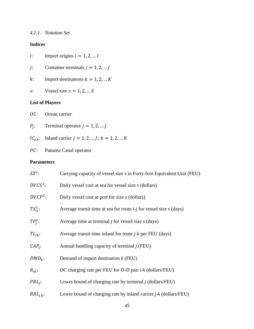
4.2.1. Notation Set

Indices

𝑖: Import origins 𝑖 = 1, 2, … 𝐼

𝑗: Container terminals 𝑗 = 1, 2, … 𝐽

𝑘: Import destinations 𝑘 = 1, 2, …𝐾

𝑠: Vessel size 𝑠 = 1, 2, … 𝑆

List of Players

𝑂𝐶: Ocean carrier

𝑃𝑗: Terminal operator 𝑗 = 1, 2, … 𝐽

𝐼𝐶𝑗,𝑘: Inland carrier 𝑗 = 1, 2, … 𝐽; 𝑘 = 1, 2, …𝐾

𝑃𝐶: Panama Canal operator

Parameters

𝑆𝑍𝑠: Carrying capacity of vessel size s in Forty-foot Equivalent Unit (FEU)

𝐷𝑉𝐶𝑆𝑆: Daily vessel cost at sea for vessel size s (dollars)

𝐷𝑉𝐶𝑃𝑆: Daily vessel cost at port for size s (dollars)

𝑇𝑆𝑖𝑗𝑠 : Average transit time at sea for route i-j for vessel size s (days)

𝑇𝑃𝑗𝑠: Average time at terminal j for vessel size s (days)

𝑇𝐿𝑗𝑘: Average transit time inland for route j-k per FEU (days)

𝐶𝐴𝑃𝑗: Annual handling capacity of terminal j (FEU)

𝐷𝑀𝐷𝑘: Demand of import destination k (FEU)

𝑅𝑖𝑘: OC charging rate per FEU for O-D pair i-k (dollars/FEU)

𝑃𝑅𝐿𝑗: Lower bound of charging rate by terminal j (dollars/FEU)

𝑅𝑅𝐿𝑗,𝑘: Lower bound of charging rate by inland carrier j-k (dollars/FEU)

45

𝐶𝑅𝐿: Lower bound of charging rate by Panama Canal (dollars/FEU)

𝑃𝑅𝑈𝑗: Upper bound of charging rate by terminal j (dollars/FEU)

𝑅𝑅𝑈𝑗,𝑘: Upper bound of charging rate by inland carrier j-k (dollars/FEU)

𝐶𝑅𝑈: Upper bound of charging rate by Panama Canal (dollars/FEU)

Decision Variables

𝑣𝑖𝑗𝑠 : Number of size s vessels on route i-j per year

𝑣𝑙𝑗,𝑘: Number of FEU shipments on route j-k per year

𝑝𝑟𝑗: Service charge per FEU by terminal j (dollars/FEU)

𝑟𝑟𝑗,𝑘: Service charge per FEU by land carrier on route j-k (dollars/FEU)

𝑐𝑟: Service charge per FEU by Panama Canal (dollars/FEU)

4.2.2. List of Functions

Revenue Function of Terminal 𝑷𝒋

𝑅𝑃𝑗�𝑝𝑟𝑗 , 𝑣𝑖𝑗𝑠 � = 𝑝𝑟𝑗 ∗ ∑ �𝑣𝑖𝑗𝑠 ∗ 𝑆𝑍𝑠�𝑠,𝑖 , 𝑗 = 1, … , 𝐽 (4.1)

Revenue function of Inland Carrier 𝑰𝑪𝒋,𝒌

𝑅𝐼𝐶𝑗,𝑘�𝑟𝑟𝑗,𝑘, 𝑣𝑙𝑗,𝑘� = 𝑟𝑟𝑗,𝑘 ∗ 𝑣𝑙𝑗,𝑘, 𝑗𝑘 = 1, … , 𝐽 ∗ 𝐾 (4.2)

Revenue function of the Panama Canal

𝑅𝑝𝑐�𝑐𝑟, 𝑣𝑖𝑗′𝑠 � = 𝑐𝑟 ∗ ∑ �𝑣𝑖𝑗′

𝑠 ∗ 𝑆𝑍𝑠�𝑠,𝑖,𝑗′ , 𝑓𝑜𝑟 𝑡𝑒𝑟𝑚𝑖𝑛𝑎𝑙 𝑗′ 𝑜𝑛 𝑡ℎ𝑒 𝐸𝑎𝑠𝑡 𝐶𝑜𝑎𝑠𝑡 (4.3)

Revenue function of Ocean Carrier

𝑅𝑜𝑐 = ∑ 𝐷𝑀𝐷𝑘 ∗ 𝑅𝑖𝑘𝑖,𝑘 (4.4)

Cost function of Terminal 𝑷𝒋

𝐶𝑃𝑗�𝑣𝑖𝑗𝑠 � = 𝑃𝑅𝐿𝑗 ∗ ∑ �𝑣𝑖𝑗𝑠 ∗ 𝑆𝑍𝑠�𝑠,𝑖 , 𝑗 = 1. . 𝐽 (4.5)

46

Cost function of Inland Carrier 𝑰𝑪𝒋,𝒌

𝐶𝐼𝐶𝑗,𝑘�𝑣𝑖𝑗𝑠 � = 𝑅𝑅𝐿𝑗,𝑘 ∗ 𝑣𝑙𝑗,𝑘, 𝑗𝑘 = 1, … , 𝐽 ∗ 𝐾 (4.6)

Cost function of the Panama Canal

𝐶𝑝𝑐�𝑣𝑖𝑗𝑠 � = 𝐶𝑅𝐿 ∗ ∑ �𝑣𝑖𝑗′𝑠 ∗ 𝑆𝑍𝑠�𝑠,𝑖,𝑗′ , 𝑓𝑜𝑟 𝑡𝑒𝑟𝑚𝑖𝑛𝑎𝑙 𝑗′ 𝑜𝑛 𝑡ℎ𝑒 𝐸𝑎𝑠𝑡 𝑐𝑜𝑎𝑠𝑡 (4.7)

Operating Cost Function of Ocean Carrier

𝐶𝑜𝑐�𝑣𝑖𝑗𝑠 � = 𝐶𝑆𝑇𝑆𝑉 + 𝐶𝑆𝑇𝑃𝑉 (4.8)

1. Total annual vessel cost at sea

𝐶𝑆𝑇𝑆𝑉 = ∑ �𝐷𝑉𝐶𝑆𝑆 ∗ 𝑇𝑆𝑖𝑗𝑠 ∗ 𝑣𝑖𝑗𝑠 �𝑠,𝑖,𝑗 (4.9)

2. Total annual vessel cost at terminal

𝐶𝑆𝑇𝑃𝑉 = ∑ �𝐷𝑉𝐶𝑃𝑆 ∗ 𝑇𝑃𝑖𝑗𝑠 ∗ 𝑣𝑖𝑗𝑠 �𝑠,𝑖,𝑗 (4.10)

Profit function of Terminal 𝑷𝒋

𝑓𝑃𝑗�𝑝𝑟𝑗, 𝑣𝑖𝑗𝑠 � = �𝑝𝑟𝑗 − 𝑃𝑅𝐿𝑗� ∗ ∑ �𝑣𝑖𝑗𝑠 ∗ 𝑆𝑍𝑠�𝑠,𝑖 , 𝑗 = 1, … , 𝐽 (4.11)

Profit function of Inland Carrier 𝑰𝑪𝒋,𝒌

𝑓𝐼𝐶𝑗,𝑘�𝑟𝑟𝑗,𝑘, 𝑣𝑙𝑗,𝑘� = �𝑟𝑟𝑗,𝑘 − 𝑅𝑅𝐿𝑗,𝑘� ∗ 𝑣𝑙𝑗,𝑘, 𝑗𝑘 = 1, … , 𝐽 ∗ 𝐾 (4.12)

Profit function of the Panama Canal

𝑓𝑝𝑐�𝑐𝑟, 𝑣𝑖𝑗′𝑠 � = (𝑐𝑟 − 𝐶𝑅𝐿) ∗ ∑ �𝑣𝑖𝑗′

𝑠 ∗ 𝑆𝑍𝑠�𝑠,𝑖,𝑗′ (4.13)

4.3. Illustration of Example Models

There are numerous possible coalitions with n players in the game, and it is impossible to

present all of them. For illustration purposes, two examples are given in this section.

The first one is that, when the grand coalition is formed, all players act as one entity and

have one common objective function of maximizing the total profit. Payments from the OC to

47

terminal operators and land carriers become “side payments” and are determined by negotiation

inside the coalition. For the grand coalition, the mathematical model will only have one level,

and its objective function is as follows:

𝑀𝑎𝑥 𝑣 = 𝑅𝑜𝑐 − 𝐶𝑜𝑐�𝑣𝑖𝑗𝑠 �. (4.14)

The second example (Model Example 2) assumes that the ocean carrier forms a coalition

with all the terminal and inland operators, while the Panama Canal is left out as a singleton

player. Thus, the first-level coalition (the leader coalition) is {𝑂𝐶,𝑃1, …𝑃𝐽, 𝐼𝐶1,1 … 𝐼𝐶𝐽𝐾}. The

second-level coalition (the follower coalition) is {𝑃𝐶}. Because members in the same coalition

essentially act as one player against the other coalition, the two coalitions’ values are determined

by competition between them while the final payment to each individual player is determined by

negotiation results inside each coalition. For simplification, the constraint set for Model Example

2 is represented by 𝑔𝑚�𝑣𝑖𝑗𝑠 , 𝑐𝑟� and ℎ𝑛�𝑣𝑖𝑗𝑠 , 𝑐𝑟�. (Detailed constraints will be explained in

Chapter 5 for the Case Study.) The coalition value of {𝑂𝐶,𝑃1, …𝑃𝐽 , 𝐼𝐶1,1 … 𝐼𝐶𝐽,𝐾} is the optimal

value of v1, and the coalition value of {𝑃𝐶} is the optimal value of v2.

4.3.1. Model Example 2

𝑀𝑎𝑥 𝑣1�𝑣𝑖𝑗𝑠 , 𝑐𝑟� = 𝑅𝑜𝑐 − 𝐶𝑜𝑐�𝑣𝑖𝑗𝑠 � − ∑ 𝐶𝑃𝑗�𝑣𝑖𝑗𝑠 �𝑗 − ∑ 𝐶𝐼𝐶𝑗,𝑘�𝑣𝑖𝑗

𝑠 �𝑗,𝑘 − 𝐶𝑝𝑐�𝑣𝑖𝑗𝑠 � − 𝑓𝑝𝑐(𝑐𝑟)

(4.15)

Subject to

𝑀𝑎𝑥 𝑣2�𝑐𝑟, 𝑣𝑖𝑗𝑠 � = 𝑓𝑝𝑐�𝑐𝑟, 𝑣𝑖𝑗𝑠 � (4.16)

Subject to

𝑔𝑚�𝑣𝑖𝑗𝑠 , 𝑐𝑟� ≤ 0,𝑚 = 1, …𝑀 (4.17)

ℎ𝑛�𝑣𝑖𝑗𝑠 , 𝑐𝑟� = 0,𝑛 = 1, …𝑁 (4.18)

48

4.4. KKT Transformation of the Bi-Level Model

The Stackelberg game is solved by first applying the Karush-Kuhn-Tucker (KKT)

conditions to the second level of the mathematical models so that the bi-level model is converted

to a single-level model. The new model is non-convex, and the global optimum may not be

found using local optimum solutions. Using the Model Example 2, the process is illustrated as

follows.

4.4.1. Original Model Example Model 2

𝑀𝑎𝑥 𝑣1(𝑣𝑖𝑗𝑠 , 𝑐𝑟) (4.19)

Subject to

𝑀𝑎𝑥 𝑣2(𝑣𝑖𝑗𝑠 , 𝑐𝑟) (4.20)

Subject to

𝑔𝑚�𝑣𝑖𝑗𝑠 , 𝑐𝑟� ≤ 0, 𝑚 = 1, … ,𝑀 (4.21)

ℎ𝑛�𝑣𝑖𝑗𝑠 , 𝑐𝑟� = 0, 𝑛 = 1, … ,𝑁 (4.22)

4.4.2. Transfer the Second level by KKT

𝑀𝑎𝑥 𝑣1�𝑣𝑖𝑗𝑠 , 𝑐𝑟� (4.23)

Subject to

𝛻𝑐𝑟𝑣2(𝑣𝑖𝑗𝑠 , 𝑐𝑟) + ∑ 𝑢𝑚 ∗ 𝛻𝑐𝑟𝑔𝑚�𝑣𝑖𝑗𝑠 , 𝑐𝑟�𝑚∈𝐴𝑐𝑡𝑖𝑣𝑒 + ∑ 𝑣𝑛 ∗ 𝛻𝑐𝑟ℎ𝑛�𝑣𝑖𝑗𝑠 , 𝑐𝑟�𝑝𝑛=1 = 0 (4.24)

𝑔𝑚�𝑣𝑖𝑗𝑠 , 𝑐𝑟� ≤ 0, 𝑚 = 1, … ,𝑀 (4.25)

ℎ𝑛�𝑣𝑖𝑗𝑠 , 𝑐𝑟� = 0, 𝑛 = 1, … ,𝑁 (4.26)

𝑢𝑚 ∗ 𝑔𝑚�𝑣𝑖𝑗𝑠 , 𝑐𝑟� = 0, 𝑚 = 1, … ,𝑀 (4.27)

𝑢𝑚 ≥ 0, 𝑚 = 1, … ,𝑀 (4.28)

49

5. CASE STUDY

As shown in the previous chapter, the complexity of the mathematical problem arises

exponentially with the number of players. This chapter creates a case study with one ocean

carrier, two terminals, one rail operator, and one Panama Canal operator. Section 5.1 explains

how the case study is established, presents Model 1 for one coalition type, and shows how Model

1 is transformed to a single-level model. The list of all 32 coalitions and their according models

are inserted as Appendix B. Section 5.2 discusses the sources and estimates for parameter values.

Model results and sensitivity analysis are presented in the next chapter.

5.1. Coalitions and Models

The five players in the case study are: one ocean carrier (OC), one terminal operator at

the Los Angles Port (P1), one terminal operator at the Norfolk Port (P2), one rail operator (R),

and one Panama Canal operator (PC). The port of Hong Kong is used as the origin, and Norfolk,

VA, is assumed as the destination. The OC has two route choices: the West Coast route (WCR),

which involves P1 and the railroad connection (R) from P1 to final destination; and the East

Coast route (ECR), which bypasses Norfolk Port and the Panama Canal. The destination is

chosen to be very near P2 so that no additional inland carrier is included for the ECR. Trucking

service is only used for the final door-delivery for both routes, and therefore, is not considered in

the game.

Because the maximum vessel size that could be handled by the Panama Canal currently is

4,400 TEUs, the vessel operating cost for the ECR is first calculated based on 4,000-TEU vessels’

normal operations, while a standard 8,000-TEU vessel is assumed for the WCR. The Panama

Canal expansion is expected to be accomplished by August 2014, and the new locks will be able

50

to handle vessels up to 13,000 TEU in capacity. By then, it is also expected both ports could

serve larger vessels like PostPanama container ships. For the case study, instead of using

variables for the number of different vessels, the variables for the shipment volume in FEU

(𝑓𝑒𝑢𝑗for port j) are used. And the number of vessels calling at terminal j can be represented by

𝑓𝑒𝑢𝑗 𝑆𝑍𝑠⁄ . Note fractional vessel numbers are accepted for this case study because, in reality,

only a portion of the containers carried by a vessel are for one destination.

The total number of coalitions is 32 (25) with five players in the game. To get the

characteristic functions and values of the 32 coalitions, 16 bi-level models are needed. The first

level of the bi-level model is for the leader coalition of OC and any of its partners, while the

second level is for the follower coalition of all the other players. Each bi-level model has a pair

of unique objective functions and a set of constraints, but all the models’ structures are similar

and could be represented by the same list of notations and functions. The 16 models and their

constraint sets are listed in Appendix A. For the 16 models, the ith model is recorded as Mi. And

𝑣𝑖1 and 𝑣𝑖2 are used to represent the 1st-level and 2nd-level objective functions of Mi, respectively.

In the following sub-sections, one type of the cooperation schemes (coalition {OC, P1}

against coalition {P2, PC, R}) is used to illustrate how a bi-level model (Model 1) should be

constructed for it and how Model 1 is transferred to one level using KKT conditions. Notations

from Chapter 3 and 4 will be continually used.

5.1.1. Model 1 Illustration

𝑀𝑎𝑥 𝑣11 = 𝑅𝑜𝑐 − 𝐶𝑜𝑐 − 𝐶𝑝1 − 𝑅𝑝2 − 𝑅𝑝𝑐 − 𝑅𝑟 = ∑ 𝑅𝑗 ∗ 𝑓𝑒𝑢𝑗𝑗 − ∑ �𝐷𝑉𝐶𝑆𝑠 ∗ 𝑇𝑆𝑗𝑠 ∗𝑗,𝑠

𝑓𝑒𝑢𝑗𝑆𝑍𝑠

� − ∑ �𝐷𝑉𝐶𝑃𝑠 ∗ 𝑇𝑃𝑗𝑠 ∗𝑓𝑒𝑢𝑗𝑆𝑍𝑠

�𝑗 − 𝑃𝑅𝐿1 ∗ 𝑓𝑒𝑢1 − 𝑝𝑟2 ∗ 𝑓𝑒𝑢2 − 𝑐𝑟 ∗ 𝑓𝑒𝑢2 − 𝑟𝑟 ∗ 𝑓𝑒𝑢1

(5.1)

Subject to

51

∑ �𝑓𝑒𝑢𝑗�𝑗 ≥ 𝐷𝑀𝐷 (5.2)

𝑓𝑒𝑢𝑗 ≤ 𝐶𝑎𝑝(𝑗),∀𝑗 (5.3)

𝑓𝑒𝑢𝑗 ≥ 0,∀𝑗 (5.4)

𝑀𝑎𝑥 𝑣12 = 𝑓𝑝2 + 𝑓𝑝𝑐 + 𝑓𝑟 = (𝑝𝑟2 − 𝑃𝑅𝐿2) ∗ 𝑓𝑒𝑢2 − (𝑐𝑟 − 𝐶𝑅𝐿) ∗ 𝑓𝑒𝑢2 − (𝑟𝑟 − 𝑅𝑅𝐿) ∗

𝑓𝑒𝑢1 (5.5)

Subject to

𝑃𝑅𝐿2 ≤ 𝑝𝑟2 ≤ 𝑃𝑅𝑈2 (5.6)

𝑅𝑅𝐿 ≤ 𝑟𝑟 ≤ 𝑅𝑅𝑈 (5.7)

𝐶𝑅𝐿 ≤ 𝑐𝑟 ≤ 𝐶𝑅𝑈 (5.8)

Equation 5.1 is total profit function of the coalition {OC, P1}, which is a function of

OC’s revenue minus total vessel operating cost, container handling cost at P1, and OC’s

payments to P2, PC, and railroad. Equations 5.2 to 5.3 are demand and capacity constraints.

Equation 5.5 is the 2nd-level objective function—the total profit function of coalition {P2, PC, R}.

It is a function of rates and shipment volume. The constraints at the second level set the upper

and lower bounds for the rate variables. The Lagrangian function of the 2nd-level problem is

given as below.

𝐿(𝑝𝑟2, 𝑐𝑟, 𝑟𝑟) = (𝑝𝑟2 − 𝑃𝑅𝐿2)𝑓𝑒𝑢2 − (𝑐𝑟 − 𝐶𝑅𝐿)𝑓𝑒𝑢2 − (𝑟𝑟 − 𝑅𝑅𝐿)𝑓𝑒𝑢1 +

𝑢1(𝑝𝑟2 − 𝑃𝑅𝐿2 − 𝑠12) + 𝑢2(𝑃𝑅𝑈2 − 𝑝𝑟2 − 𝑠22) + 𝑢3(𝑟𝑟 − 𝑅𝑅𝐿 − 𝑠32) + 𝑢4(𝑅𝑅𝑈 − 𝑟𝑟 − 𝑠42) +

𝑢5(𝑐𝑟 − 𝐶𝑅𝐿 − 𝑠52) + 𝑢6(𝐶𝑅𝑈 − 𝑐𝑟 − 𝑠62) (5.9)

Using the Karush-Kuhn-Tucker (KKT) transformation, the new single-level model is

shown by Equations 5.10 to 5.21.

52

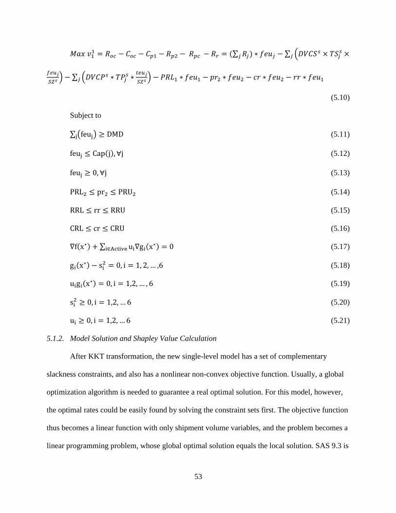
𝑀𝑎𝑥 𝑣11 = 𝑅𝑜𝑐 − 𝐶𝑜𝑐 − 𝐶𝑝1 − 𝑅𝑝2 − 𝑅𝑝𝑐 − 𝑅𝑟 = (∑ 𝑅𝑗) ∗ 𝑓𝑒𝑢𝑗𝑗 − ∑ �𝐷𝑉𝐶𝑆𝑠 × 𝑇𝑆𝑗𝑠 ×𝑗

𝑓𝑒𝑢𝑗𝑆𝑍𝑠

� − ∑ �𝐷𝑉𝐶𝑃𝑠 ∗ 𝑇𝑃𝑗𝑠 ∗𝑡𝑒𝑢𝑗𝑆𝑍𝑠

�𝑗 − 𝑃𝑅𝐿1 ∗ 𝑓𝑒𝑢1 − 𝑝𝑟2 ∗ 𝑓𝑒𝑢2 − 𝑐𝑟 ∗ 𝑓𝑒𝑢2 − 𝑟𝑟 ∗ 𝑓𝑒𝑢1

(5.10)

Subject to

∑ �feuj�j ≥ DMD (5.11)

feuj ≤ Cap(j),∀j (5.12)

feuj ≥ 0,∀j (5.13)

PRL2 ≤ pr2 ≤ PRU2 (5.14)

RRL ≤ rr ≤ RRU (5.15)

CRL ≤ cr ≤ CRU (5.16)

∇f(x∗) + ∑ ui∇gi(x∗)i∈Active = 0 (5.17)

gi(x∗) − si2 = 0, i = 1, 2, … ,6 (5.18)

uigi(x∗) = 0, i = 1,2, … , 6 (5.19)

si2 ≥ 0, i = 1,2, … 6 (5.20)

ui ≥ 0, i = 1,2, … 6 (5.21)

5.1.2. Model Solution and Shapley Value Calculation

After KKT transformation, the new single-level model has a set of complementary

slackness constraints, and also has a nonlinear non-convex objective function. Usually, a global

optimization algorithm is needed to guarantee a real optimal solution. For this model, however,

the optimal rates could be easily found by solving the constraint sets first. The objective function

thus becomes a linear function with only shipment volume variables, and the problem becomes a

linear programming problem, whose global optimal solution equals the local solution. SAS 9.3 is

53

applied to solve all 16 models. Based on Equation 3.8, each player’s Shapley value calculation is

presented in Equation 5.22 to Equation 5.26.

Terminal 1’s Shapley Value:

∅P1 = 4!0!5!

(v151 − v141 ) + 3!1!5!

(v131 − v101 ) + 3!1!5!

(v121 − v91) + 3!1!5!

(v111 − v81) +

3!1!5!

(v02 − v12) + 2!2!5!

(v71 − v41) + 2!2!5!

(v61 − v31) + 2!2!5!

(v51 − v21) + 2!2!5!

(v42 − v72) + 2!2!5!

(v32 −

v62) + 2!2!5!

(v22 − v52) + 3!1!5!

(v11 − v01) + 3!1!5!

(v82 − v112 ) + 3!1!5!

(v92 − v122 ) + 3!1!5!

(v102 − v132 ) +

4!5!

(v142 − v152 ) (5.22)

Terminal 2’s Shapley Value:

∅P2 = 4!0!5!

(v151 − v131 ) + 3!1!5!

(v141 − v101 ) + 3!1!5!

(v121 − v71) + 3!1!5!

(v111 − v61) +

3!1!5!

(v02 − v22) + 2!2!5!

(v91 − v41) + 2!2!5!

(v81 − v31) + 2!2!5!

(v51 − v11) + 2!2!5!

(v42 − v92) + 2!2!5!

(v32 −

v82) + 2!2!5!

(v12 − v52) + 3!1!5!

(v21 − v01) + 3!1!5!

(v62 − v112 ) + 3!1!5!

(v72 − v122 ) + 3!1!5!

(v102 − v142 ) +

4!5!

(v132 − v152 ) (5.23)

Panama Canal’s Shapley value:

∅PC = 4!0!5!

(v151 − v121 ) + 3!1!5!

(v141 − v91) + 3!1!5!

(v131 − v71) + 3!1!5!

(v111 − v51) +

3!1!5!

(v02 − v32) + 2!2!5!

(v101 − v41) + 2!2!5!

(v81 − v21) + 2!2!5!

(v61 − v11) + 2!2!5!

(v42 − v102 ) +

2!2!5!

(v22 − v82) + 2!2!5!

(v12 − v62) + 3!1!5!

(v31 − v01) + 3!1!5!

(v52 − v112 ) + 3!1!5!

(v72 − v132 ) +

3!1!5!

(v92 − v142 ) + 4!5!

(v122 − v152 ) (5.24)

54

Railway’s Shapley value:

∅R = 4!0!5!

(v151 − v111 ) + 3!1!5!

(v141 − v81) + 3!1!5!

(v131 − v61) + 3!1!5!

(v121 − v51) +

3!1!5!

(v02 − v42) + 2!2!5!

(v101 − v31) + 2!2!5!

(v91 − v21) + 2!2!5!

(v71 − v11) + 2!2!5!

(v32 − v102 ) +

2!2!5!

(v22 − v92) + 2!2!5!

(v12 − v72) + 3!1!5!

(v41 − v01) + 3!1!5!

(v52 − v122 ) + 3!1!5!

(v62 − v132 ) +

3!1!5!

(v82 − v142 ) + 4!5!

(v112 − v152 ) (5.25)

Ocean carrier’s Shapley value:

∅OC = 4!0!5!

(v151 − v02) + 3!1!5!

(v141 − v12) + 3!1!5!

(v131 − v22) + 3!1!5!

(v121 − v32) +

3!1!5!

(v111 − v42) + 2!2!5!

(v101 − v52) + 2!2!5!

(v91 − v62) + 2!2!5!

(v81 − v72) + 2!2!5!

(v71 − v82) +

2!2!5!

(v61 − v92) + 2!2!5!

(v51 − v102 ) + 3!1!5!

(v41 − v112 ) + 3!1!5!

(v31 − v122 ) + 3!1!5!

(v21 − v132 ) +

3!1!5!

(v11 − v142 ) + 4!5!

(v01 − v152 ) (5.26)

5.2. Parameter Estimates

5.2.1. Daily Vessel Operating Cost

Vessel operating cost is a function of shipping speed, fuel consumption rate, and other

variable costs, including fuel, crew, maintenance, and administration costs. The Army Corps of

Engineers Aggregated Vessel Operating Cost Model (AVOCM) has input values regarding ship

size, speed, fuel usage rate, and average opportunity cost of capital, as well as other endogenized

costs like insurance and operating cost (Army Corps of Engineers 2007). Fan (2010) used daily

charter rates to replace AVCOM’s fixed capital asset and operating costs and derived the

estimation functions for the daily vessel operating cost (Equations 6.27 and 6.28). This study re-

estimates the vessel operating costs using updated fuel prices and daily hire rates from the

Bloomberg Professional Service database (Bloomberg L. P. 2013a, b).

55

𝐷𝑉𝐶𝑆𝑠 = 𝐴𝑈𝑠 ∗ 𝑀𝐷𝑂 + 𝐸𝐶𝑠 ∗ 𝐻𝑉𝑂 + 𝐷𝐻𝑖𝑟𝑒𝑟𝑎𝑡𝑒𝑠 (5.27)

𝐷𝑉𝐶𝑃𝑠 = 𝐴𝑈𝑠 ∗ 𝑀𝐷𝑂 + 𝐷𝐻𝑖𝑟𝑒𝑟𝑎𝑡𝑒𝑠 (5.28)

𝐷𝑉𝐶𝑆𝑠: Daily vessel cost at sea for container vessel of size s (dollars)

𝐷𝑉𝐶𝑃𝑠: Daily vessel cost at port for container vessel of size s (dollars)

𝐴𝑈𝑠: Bunkerage consumption rate for auxiliary power generation for container

vessel of size s (metric tons/day)

𝐸𝐶𝑠: Bunkerage consumption rate for propulsion mover(s) for container vessel

of size s at economic speed (metric tons/day)

𝑀𝐷𝑂: Marine diesel oil price (dollars/metric ton)

𝐻𝑉𝑂: Heavy viscosity oil price (dollars/metric ton)

𝐷𝐻𝑖𝑟𝑒𝑟𝑎𝑡𝑒𝑠: Daily charter rate of container vessel of size s (dollars/day)

The values of economic speed and engine fuel consumption rates for different container

ship sizes are available from AVOCM. Only 4,000-TEU and 8,000-TEU vessels are used in the

case study (Table 5.1). Fuel prices fluctuate vastly through time. Figure 5.1 shows the HVO and

MDO price changes from April 2010 to March 2013. The average price from 2010 to 2012 based

on the Los Angeles price (Bloomberg L. P. 2013a) is used: $917 per metric ton for MDO and

$603 per metric ton for HVO (380 centistokes).

Table 5.1. Fuel Consumption Rates and Economic Speeds of the Vessels Vessel Category

Vessel size (TEU)

AU (MT/Day)

EC (MT/Day)

Economic Speed (NM/Hour)

Panamax 4,000 3.9 103.2 21.3 PostPanamax 8,000 5.2 202.6 25

56

Figure 5.1. HVO and MDO Price Changes

Figure 5.2. Daily Hire Rates Changes

The daily hire rate changes for vessel sizes of 11,100 TEU, 1,700 TEU, 2,500 TEU,

3,500 TEU, and 4,250 TEU from 2010 to 2012 are shown in Figure 5.2 (Bloomberg L. P. 2013a).

57

The average values from 2010 to 2012 are used to estimate a regression function of daily hire

rates on vessel size s (Equation 6.29). The estimated values of a and b are 30 and 0.7672. The

estimation R2 is 0.97 (Figure 5.3). The daily hire rates for the vessels for different vessel sizes

are predicted using the regression function. Daily hire rate is estimated as $16,820 for a 4,000-

TEU vessel and $28,627 for an 8,000-TEU vessel.

𝐷𝐻𝑖𝑟𝑒𝑟𝑎𝑡𝑒𝑠 = 𝑎 ∗ 𝑠𝑏 (5.29)

Figure 5.3. Daily Hire Rates Estimation

5.2.2. Transit Time Estimates

Container terminals usually operate approximately 28 to 35 moves per crane per hour at

top North American ports (Le-Griffin and Murphy 2006). Container productivity is critical for

container ports like LA and NF. Thus, it is assumed both terminals in the case have the capacity

58

to efficiently handle the PostPanama vessels, and there will be no difference between the two

ports’ vessel handling time. With three cranes with 35 moves per crane per hour serving a vessel

with a capacity of 8,000 TEU and a loading factor of 0.8, it takes about 2.5 days to off-load the

vessel. With two cranes with 30 moves per crane per hour serving a vessel with capacity of 4,000

TEU and loading factor of 0.8, it takes about 2.2 days. Considering other activities (paperwork,

waiting, supply, etc.) that further cost more time, the total port time is estimated as three days for

the PostPanamax vessel (8,000 TEU) and 2.5 days for the Panamax vessel (4,000 TEU).

Additional days are needed when the Panama Canal is used for the ECR. The Canal uses

two quality service-level indicators: 1) average waiting time to transit the Canal; and 2) average

transit time. Their combination is called Canal Waters Time (CWT) (Panama Canal Authority

2006). On average, the transit time takes eight to 10 hours to go through the Canal (Panama

Canal Authority 2010). The waiting time could vary depending on the congestion condition and

whether a transit is reserved beforehand. Typically, the reserved CWT is about 17 hours (0.7

days) versus 36 hours (1.5 days) for non-reserved (Wilson, Dahl, and Fan 2010). For the ECR,

1.5 days are added to port time. The time at sea is calculated using economic speeds from the

AVOCM model for each vessel size (Army Corps of Engineers 2007). Table 5.2 lists the

economic speed, port distance overseas, traveling time at sea, and time at port used in the case

study.

Table 5.2. Vessel Time Estimates

Economic Speed

(nautical miles/hour)

Sea Distance (nautical miles)

Time at Sea (days)

Time at Port (days)

LA 8,000 TEU 25 7,455 10.6 3 NF 8,000 TEU 25 12,883 18.4 4.5 NF 4,000 TEU 21.3 12,883 21.6 4

Sources: Data from Fan (2010) and Army Corps of Engineers (2007).

59

The railway shipment time from LA to Norfolk, VA, is calculated from two segments:

LA to Chicago and Chicago to Norfolk. Based on the two segments’ estimated shipment time

(Table 5.3), the total inland container transit time is estimated to be four days for LA to Norfolk,

VA. The transit time from Norfolk to VA is assumed to be 0.5 days. It is assumed that

cooperation between any transportation operator (the terminal, the Panama Canal, or the railroad)

and the OC will save the OC half a day of normal transit time.

Table 5.3. Container Inland Time Estimates for WCR

Railway Company Mileage Speed

(mph) Days

LA to Chicago BNSF 2,161 36 2.5 Chicago to Norfolk, VA CSX 964 30 1.34 Source: Data from Fan (2010).

5.2.3. Inventory Cost

Other than transportation cost paid directly to carriers, another major cost sector for

shippers is the opportunity cost of working capital tied up in the inventory throughout the supply

chain. Although it is assumed that the OC chooses the optimal routes to maximize its profit and

that inventory costs are not directly reflected in the OC’s profit function, the difference of the

transit time has implicit impact on the OC’s route choice. To reflect shippers’ perceptions of

shipping speed, different charging rates of the OC are assumed. The OC’s charging rate R1 for a

quicker route (WCR in this case) is set to be higher than R2 for the slower ECR. The reason is

that quicker delivery saves shippers inventory cost. To estimate the difference between the two

rates, Equation 6.30 is derived based on Wardrop’s First Principle. At equilibrium, both routes

should have equalized lowest cost for the shippers. Irt is the inventory cost for route rt (rt = 1 or

2).

𝑅1 + 𝐼1 = 𝑅2 + 𝐼2 (5.30)

60

There are three types of inventories in a supply chain: cycle inventory, safety stock, and

pipeline inventory. Cycle inventory is a function of the replenishment frequency and is

independent of the selection of the route, and therefore is irrelevant for route choices. Safety

stock is the extra inventory kept to satisfy the customer demand on time. It is a function of the

customer service level, the uncertainties in the shipment lead time, and the demand forecast error

(Jula and Leachman 2011a). Assuming demand is deterministic and there is no shipment

uncertainty, safety stock is not considered as well. Pipeline inventory is the amount of inventory

in transit. The annual inventory cost per unit is a function of the transportation time and daily

unit pipeline inventory cost (DPC) (Equation 6.31). DPC is calculated as an inventory carrying

rate (annual interest rate for commercial loans) times the amount of capital invested per unit of

inventory (Equation 6.32).

𝐼𝑟𝑡 = 𝐷𝑃𝐶 ∗ 𝑇𝑟𝑡 (5.31)

𝐷𝑃𝐶 = 𝑟 ∗ 𝑈𝑉/365 (5.32)

𝐼𝑟𝑡: Total annual pipeline inventory cost per FEU for route rt (dollars)

𝐷𝑃𝐶: Daily pipeline inventory cost per FEU (dollars)

𝑇𝑟𝑡: Transit time per FEU for route rt (days)

𝑟: Annual interest rate

𝑈𝑉: Average cargo value per FEU (dollars)

Jula and Leachman (2011b) suggest a 20% inventory carrying rate per year for

replenishment of goods with long-term demand, and 50% if retail prices are declining with time

or if the products experience rapid obsolescence. An average inventory carrying rate of 35% is

assumed for simplicity. Using joint data from PIERS database, World Trade Atlas (WTA)

database, and Pacific Maritime Association’s database, Leachman (2010) calculated the average

61

declared values per cubic foot for containerized imports from Asia to different coast ports in the

United States (Table 5.4). The average cargo value per FEU (UV) is estimated assuming the

average usable space is about 2,684 cubic feet for a high-cube 40-foot container (9.5-foot high

and 40-foot long). Using Equation 6.32, daily pipeline inventory cost (DPC) is estimated in

Table 5.4. Using daily pipeline inventory cost of $56.00 per day and Equation 6.30, the charging

rate difference between the two routes is calculated as 𝑅1 − 𝑅2 = 𝐼2 − 𝐼1 = 56(𝑇2 − 𝑇1).

Table 5.4. Daily Pipeline Inventory Cost Calculation Asia to U.S. Asia to West Coast Asia to East/Gulf Coast Cargo Value ($/cu ft) 21.66 22.66 18.57 UV ($/FEU) 58,135.44 60,819.44 49,841.88 DPC ($/FEU/Day) 55.75 58.32 47.79

Source: Compiled using data from Leachman (2010).

5.2.4. Transportation Rates

Shipping rates, terminal charges, canal tolls, and railway rates are all sensitive

information and very volatile through time. Spot market rates from public sources are obtained to

estimate general ranges.

5.2.4.1. Trans-Pacific shipping rates

On August 16, 2013, according to SCFI data issued by the Shanghai Shipping Exchange,

the spot rate from Shanghai to the U.S. West Coast was $1,941 per FEU, 27.7% below the level

in the same week last year and 12.6%, or $280, less than at the beginning of 2013. The spot rate

to the U.S. East Coast was $3,408 in the week ending August 16, 13.6% down from the same

week in 2012, but up 1.5%, or $50, from January 1 (Journal of Commerce 2013c). For the case

study, the shipping rate R1 charged by the OC for the all-water route (WCR) is assumed to be

$3,400 per FEU. Depending on the vessel size used for ECR, the transit time and inventory cost

differences between the two routes will be different. Using Equations 6.30, 6.31, and 6.32, the

shipping rate R2 for the transcontinental route (ECR) could be derived accordingly.

62

5.2.4.2. Railroad charging rates

The rail rate ranges are estimated based on the most current Public Use Waybill File (U.S.

Surface Transportation Board 2011), which contains sample data on rail shipments from origin

Business Economic Area (BEA) to termination BEA. Because there is no railroad company with

direct shipment from Los Angeles to Norfolk on its own network, the rail route is analyzed based

on the LA-Chicago segment (operated by BNSF) and the Chicago-Norfolk, VA, segment

(operated by CSX). The line haul rates per container are calculated using “Expanded Freight

Revenue” divided by “Expanded Trailer/Container Count” for shipments from LA (BEA = 160)

to Chicago (BEA = 64), and for shipments from Chicago to Norfolk, VA (BEA = 20). Only

containerized cargoes (STCC2 = “46”) are counted. The calculated rates are summarized in

Table 5.5.

Using the lowest record as the lower bound of railroad rates and the 90% percentile value

as the upper bound, the railroad rate for LA to Norfolk, VA, is estimated to range from $1,420 to

$3,400 per container. As the railway does not report the size of the containers, it is assumed the

majority of those are 53-foot domestic containers.

According to spot market reports, the west-to-east door-to-door spot rates in early May

2013 were about $2,300 for a 53-foot intermodal container, and the spot rate for Los Angeles-

New Jersey fell 2.4% ($80) to $3,285 in the second week of May (Journal of Commerce 2013d).

In early August, the west to east bound rate rose again to about $2,390. The largest increase in

the first week of August was the Los Angeles-Atlanta route: 2.4% ($70) to $3,000 (Journal of

Commerce 2013b). Comparing the two sources, the lower and upper bound estimates for the

railroad rates are reasonable for this study.

63

Table 5.5. Railway Shipment Rates Summary Quantile LA-Chicago Rate Chicago-NF Rate

100% Max 3670 2751

99% 2187 1835

95% 1997 1584

90% 1887 1511

75% Q3 1692 1388

50% Median 1435 1163

25% Q1 1184 1043

10% 1007 957

5% 870 901

1% 756 843

0% Min 665 756

The rates are transferred from 35-foot containers to high-cube 40-foot containers based

on the usage capacity ratios. Usable capacity for a domestic container (a 35-foot-long container)

is about 4,000 cubic feet and 2,684 cubic feet for a high-cube 40-foot container . Therefore, the

final upper and lower bounds for railroad rates for ECR are estimated as $953 per FEU and

$2,280 per FEU, respectively.

5.2.4.3. Port and Panama Canal charging rates

The average terminal handling cost for some European countries could be found through

the APL website (www.APL.com). Those rates range from $127 to $300 per container. Based on

personal communication with Chuck Raymond (former CEO of Horizon Lines, Inc.) and David

Smith (CEO of Work Cat Engineering LLC), the lowest expected container handling rate at

some terminals of the Norfolk port is about $150 per container. Assuming there is no big

difference between the two ports’ costs and charging rates, the lower and upper bounds of the

terminal charges for the case study are set as $150 and $300, respectively.

64

Compared with the other rates, the Panama Canal tolls are relatively easy to estimate. The

canal tolls were $54/TEU in 2007 and $72/TEU in 2009 and 2010. Including ancillary fees, the

total fee in 2010 is about $88/TEU if booking service is used, while about $80/TEU without

booking beforehand (Wilson, Dahl, and Fan 2010). The CEO of Maersk Line said the fees for

ships to go through the Panama Canal have tripled in the past five years to $450,000 per passage

for a vessel carrying 4,500 containers since 2009 (Park 2013). That is about $100/TEU if all the

containers are 20 feet. The lower bound of the Panama Canal rate is set as $160/FEU, and the

upper bound is set as $220/FEU.

65

6. RESULT ANALYSIS

6.1. Model Results and CGT Solutions

As stated in Chapter 5, the container vessel used for the East Coast route (ECR) is 4,000

TEU before the Panama Canal expansion is finished and 8,000 TEU after the expansion. The

West Coast route (WCR) is served by 8,000-TEU vessels both before and after the expansion.

For all ships, 80% carry capacity is assumed. The total containerized demand at the destination

(Norfolk, VA) is assumed to be 64,000 FEU annually, and is shared by the two routes. To

analyze the impact of capacity constraints, the models are both calculated with assumptions that

there are no terminal TEU capacity constraints, and with assumptions that both terminals could

only handle 80% of total container demand. Hence, in all, four scenarios are compared.

Scenario 1 (S1): “Base Case: Before Canal Expansion & No Capacity Constraints.”

Scenario 2 (S2): “After Canal Expansion & No Capacity Constraints.”

Scenario 3 (S3): “Before Canal Expansion & Capacity Constraints at Terminals.”

Scenario 4 (S4): “After Canal Expansion & Capacity Constraints at Terminals.”

The models’ results are in Appendix B Table B1, Table B2, Table B3, and Table B4. As

Model 15’s result shows, if the grand coalition is formed, the OC prefers the WCR before the

Canal expansion is finished. However, after the expansion is finished and both routes are served

by the 8,000-TEU vessel, the OC chooses ECR via the Panama Canal because of a higher profit.

The Shapley values are presented in Table 6.1. In order to compare scenarios, the ratios

of the Shapley Value are also calculated in each scenario and listed in Table 6.1. The ratios are a

reflection of players’ relative market powers under each scenario. A player’s Shapley value is the

total profit allocation for that player because the models’ objective functions are profit

maximization. The values are all divided by 64,000 for the purpose of easy presentation and

66

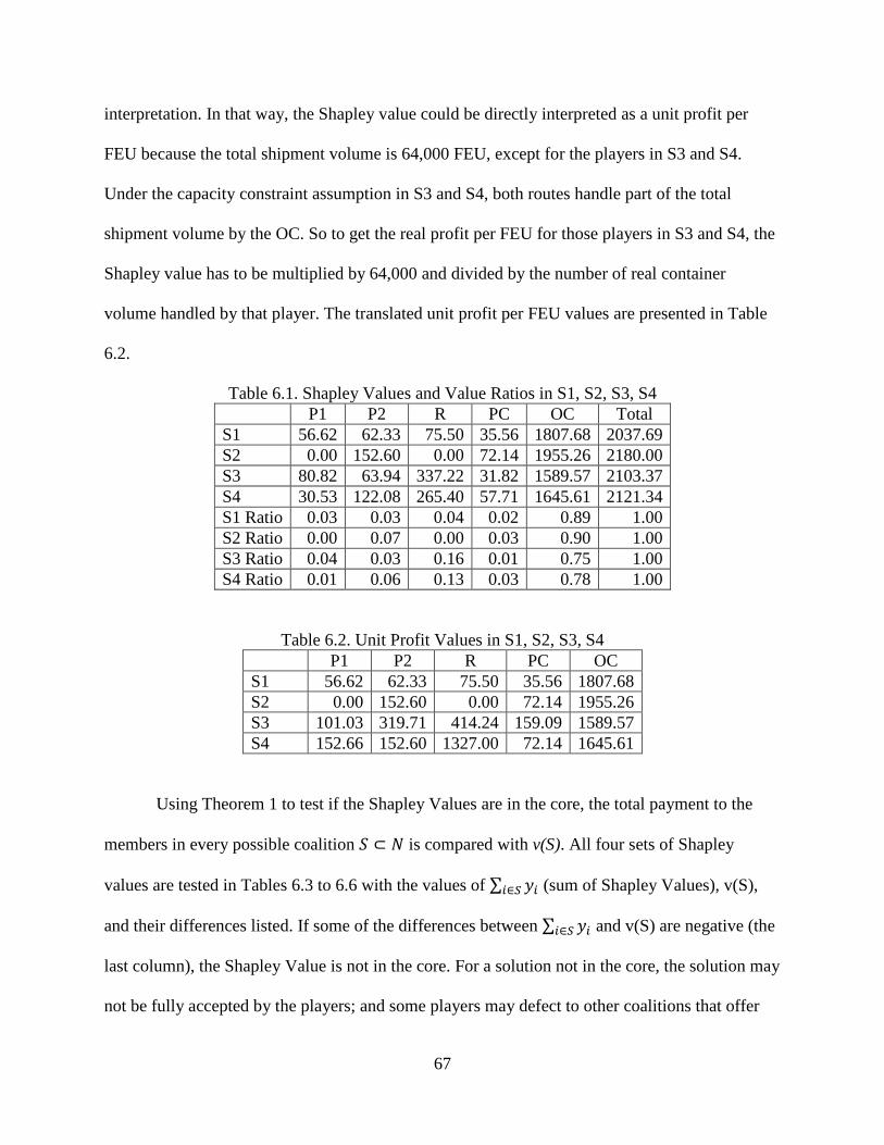
interpretation. In that way, the Shapley value could be directly interpreted as a unit profit per

FEU because the total shipment volume is 64,000 FEU, except for the players in S3 and S4.

Under the capacity constraint assumption in S3 and S4, both routes handle part of the total

shipment volume by the OC. So to get the real profit per FEU for those players in S3 and S4, the

Shapley value has to be multiplied by 64,000 and divided by the number of real container

volume handled by that player. The translated unit profit per FEU values are presented in Table

6.2.

Table 6.1. Shapley Values and Value Ratios in S1, S2, S3, S4 P1 P2 R PC OC Total S1 56.62 62.33 75.50 35.56 1807.68 2037.69 S2 0.00 152.60 0.00 72.14 1955.26 2180.00 S3 80.82 63.94 337.22 31.82 1589.57 2103.37 S4 30.53 122.08 265.40 57.71 1645.61 2121.34 S1 Ratio 0.03 0.03 0.04 0.02 0.89 1.00 S2 Ratio 0.00 0.07 0.00 0.03 0.90 1.00 S3 Ratio 0.04 0.03 0.16 0.01 0.75 1.00 S4 Ratio 0.01 0.06 0.13 0.03 0.78 1.00

Table 6.2. Unit Profit Values in S1, S2, S3, S4 P1 P2 R PC OC S1 56.62 62.33 75.50 35.56 1807.68 S2 0.00 152.60 0.00 72.14 1955.26 S3 101.03 319.71 414.24 159.09 1589.57 S4 152.66 152.60 1327.00 72.14 1645.61

Using Theorem 1 to test if the Shapley Values are in the core, the total payment to the

members in every possible coalition 𝑆 ⊂ 𝑁 is compared with v(S). All four sets of Shapley

values are tested in Tables 6.3 to 6.6 with the values of ∑ 𝑦𝑖𝑖∈𝑆 (sum of Shapley Values), v(S),

and their differences listed. If some of the differences between ∑ 𝑦𝑖𝑖∈𝑆 and v(S) are negative (the

last column), the Shapley Value is not in the core. For a solution not in the core, the solution may

not be fully accepted by the players; and some players may defect to other coalitions that offer

67

them better profits. But the Shapley value still works as a measure of relative market power of

the players, since it measures the average attribution made by each player. As Tables 6.3 to

Table 6.6 show, both S1 and S3’s Shapley values are not in the core.

Table 6.3. Coalition Values for S1

players v(S) OC P1 P2 PC R sum(yi) sum(yi) -

v(S) OC 1716.25 1807.68 1807.68 91.43 OC P1 1716.25 1807.68 56.62 1864.30 148.05 OC P2 1872.50 1807.68 62.33 1870.01 -2.49 OC PC 1801.88 1807.68 35.56 1843.24 41.37 OC R 1882.38 1807.68 75.50 1883.18 0.80 OC P1 P2 1872.50 1807.68 56.62 62.33 1926.63 54.13 OC P1 Pc 1801.88 1807.68 56.62 35.56 1899.86 97.99 OC P1 R 2037.69 1807.68 56.62 75.50 1939.80 -97.89 OC P2 PC 1958.13 1807.68 62.33 35.56 1905.57 -52.55 OC P2 R 1882.38 1807.68 62.33 75.50 1945.51 63.13 OC PC R 1882.38 1807.68 35.56 75.50 1918.74 36.36 OC P1 P2 PC 1958.13 1807.68 56.62 62.33 35.56 1962.19 4.07 OC P1 P2 R 2037.69 1807.68 56.62 62.33 75.50 2002.13 -35.56 OC P1 PC R 2037.69 1807.68 56.62 35.56 75.50 1975.36 -62.33 OC P2 PC R 1958.13 1807.68 62.33 35.56 75.50 1981.07 22.94 OC P1 P2 PC R 2037.69 1807.68 56.62 62.33 35.56 75.50 2037.69 0.00 P1 P2 PC R 210.00 56.62 62.33 35.56 75.50 230.00 20.00 P2 PC R 210.00 62.33 35.56 75.50 173.38 -36.62 P1 PC R 60.00 56.62 35.56 75.50 167.67 107.67 P1 P2 R 150.00 56.62 62.33 75.50 194.45 44.45 P1 P2 PC 150.00 56.62 62.33 35.56 154.51 4.51 PC R 60.00 35.56 75.50 111.05 51.05 P2 R 150.00 62.33 75.50 137.82 -12.18 P2 PC 0.00 62.33 35.56 97.89 97.89 P1 R 0.00 56.62 75.50 132.12 132.12 P1 PC 150.00 56.62 35.56 92.18 -57.82 P1 P2 150.00 56.62 62.33 118.95 -31.05 R 0.00 75.50 75.50 75.50 PC 0.00 35.56 35.56 35.56 P2 0.00 62.33 62.33 62.33 P1 0.00 56.62 56.62 56.62

68

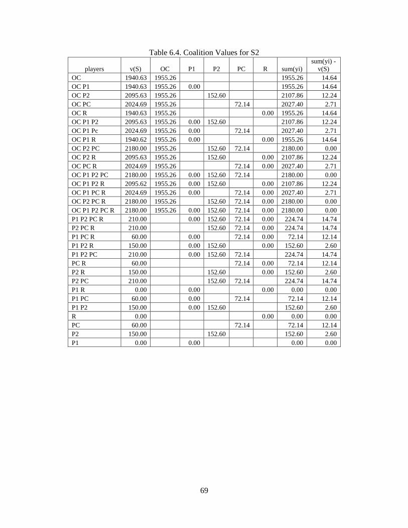
Table 6.4. Coalition Values for S2

players v(S) OC P1 P2 PC R sum(yi) sum(yi) -

v(S) OC 1940.63 1955.26 1955.26 14.64 OC P1 1940.63 1955.26 0.00 1955.26 14.64 OC P2 2095.63 1955.26 152.60 2107.86 12.24 OC PC 2024.69 1955.26 72.14 2027.40 2.71 OC R 1940.63 1955.26 0.00 1955.26 14.64 OC P1 P2 2095.63 1955.26 0.00 152.60 2107.86 12.24 OC P1 Pc 2024.69 1955.26 0.00 72.14 2027.40 2.71 OC P1 R 1940.62 1955.26 0.00 0.00 1955.26 14.64 OC P2 PC 2180.00 1955.26 152.60 72.14 2180.00 0.00 OC P2 R 2095.63 1955.26 152.60 0.00 2107.86 12.24 OC PC R 2024.69 1955.26 72.14 0.00 2027.40 2.71 OC P1 P2 PC 2180.00 1955.26 0.00 152.60 72.14 2180.00 0.00 OC P1 P2 R 2095.62 1955.26 0.00 152.60 0.00 2107.86 12.24 OC P1 PC R 2024.69 1955.26 0.00 72.14 0.00 2027.40 2.71 OC P2 PC R 2180.00 1955.26 152.60 72.14 0.00 2180.00 0.00 OC P1 P2 PC R 2180.00 1955.26 0.00 152.60 72.14 0.00 2180.00 0.00 P1 P2 PC R 210.00 0.00 152.60 72.14 0.00 224.74 14.74 P2 PC R 210.00 152.60 72.14 0.00 224.74 14.74 P1 PC R 60.00 0.00 72.14 0.00 72.14 12.14 P1 P2 R 150.00 0.00 152.60 0.00 152.60 2.60 P1 P2 PC 210.00 0.00 152.60 72.14 224.74 14.74 PC R 60.00 72.14 0.00 72.14 12.14 P2 R 150.00 152.60 0.00 152.60 2.60 P2 PC 210.00 152.60 72.14 224.74 14.74 P1 R 0.00 0.00 0.00 0.00 0.00 P1 PC 60.00 0.00 72.14 72.14 12.14 P1 P2 150.00 0.00 152.60 152.60 2.60 R 0.00 0.00 0.00 0.00 PC 60.00 72.14 72.14 12.14 P2 150.00 152.60 152.60 2.60 P1 0.00 0.00 0.00 0.00

69

Table 6.5. Coalition Values for S3

players v(S) OC P1 P2 PC R sum(yi) sum(yi) -v(S)

OC 1504.47 1589.57 1589.57 85.10 OC P1 1535.54 1589.57 80.82 1670.40 134.86 OC P2 1629.48 1589.57 63.94 1653.52 24.04 OC PC 1572.97 1589.57 31.82 1621.39 48.42 OC R 1930.75 1589.57 337.22 1926.79 -3.96 OC P1 P2 1660.54 1589.57 80.82 63.94 1734.34 73.80 OC P1 Pc 1604.04 1589.57 80.82 31.82 1702.22 98.18 OC P1 R 2055.00 1589.57 80.82 337.22 2007.62 -47.38 OC P2 PC 1697.97 1589.57 63.94 31.82 1685.33 -12.64 OC P2 R 1962.00 1589.57 63.94 337.22 1990.73 28.73 OC PC R 1947.87 1589.57 31.82 337.22 1958.61 10.73 OC P1 P2 PC 1729.04 1589.57 80.82 63.94 31.82 1766.16 37.12 OC P1 P2 R 2086.25 1589.57 80.82 63.94 337.22 2071.56 -14.69 OC P1 PC R 2072.13 1589.57 80.82 31.82 337.22 2039.43 -32.69 OC P2 PC R 1942.98 1589.57 63.94 31.82 337.22 2022.55 79.58 OC P1 P2 PC R 2103.37 1589.57 80.82 63.94 31.82 337.22 2103.37 0.00 P1 P2 PC R 463.40 80.82 63.94 31.82 337.22 513.80 50.40 P2 PC R 433.40 63.94 31.82 337.22 432.98 -0.42 P1 PC R 343.40 80.82 31.82 337.22 449.86 106.46 P1 P2 R 415.40 80.82 63.94 337.22 481.98 66.58 P1 P2 PC 162.00 80.82 63.94 31.82 176.58 14.58 PC R 313.40 31.82 337.22 369.03 55.63 P2 R 385.40 63.94 337.22 401.16 15.76 P2 PC 42.00 63.94 31.82 95.76 53.76 P1 R 295.40 80.82 337.22 418.04 122.64 P1 PC 132.00 80.82 31.82 112.64 -19.36 P1 P2 150.00 80.82 63.94 144.77 -5.23 R 265.40 337.22 337.22 71.82 PC 12.00 31.82 31.82 19.82 P2 30.00 63.94 63.94 33.94 P1 30.00 80.82 80.82 50.82

70

Table 6.6. Coalition Values for S4

players v(S) OC P1 P2 PC R sum(yi) sum(yi) -v(S)

OC 1633.37 1645.61 1645.61 12.24 OC P1 1664.44 1645.61 30.53 1676.15 11.71 OC P2 1757.38 1645.61 122.08 1767.70 10.32 OC PC 1700.62 1645.61 57.71 1703.32 2.70 OC R 1898.77 1645.61 265.40 1911.01 12.24 OC P1 P2 1788.44 1645.61 30.53 122.08 1798.23 9.79 OC P1 Pc 1731.69 1645.61 30.53 57.71 1733.85 2.17 OC P1 R 1929.84 1645.61 30.53 265.40 1941.55 11.71 OC P2 PC 1824.87 1645.61 122.08 57.71 1825.41 0.53 OC P2 R 2022.77 1645.61 122.08 265.40 2033.10 10.32 OC PC R 1966.02 1645.61 57.71 265.40 1968.72 2.70 OC P1 P2 PC 1855.94 1645.61 30.53 122.08 57.71 1855.94 0.00 OC P1 P2 R 2053.84 1645.61 30.53 122.08 265.40 2063.63 9.79 OC P1 PC R 1997.09 1645.61 30.53 57.71 265.40 1999.25 2.17 OC P2 PC R 2090.28 1645.61 122.08 57.71 265.40 2090.81 0.53 OC P1 P2 PC R 2121.34 1645.61 30.53 122.08 57.71 265.40 2121.34 0.00 P1 P2 PC R 463.40 30.53 122.08 57.71 265.40 475.72 12.32 P2 PC R 433.40 122.08 57.71 265.40 445.19 11.79 P1 PC R 343.40 30.53 57.71 265.40 353.64 10.24 P1 P2 R 415.40 30.53 122.08 265.40 418.01 2.61 P1 P2 PC 198.00 30.53 122.08 57.71 210.32 12.32 PC R 313.40 57.71 265.40 323.11 9.71 P2 R 385.40 122.08 265.40 387.48 2.08 P2 PC 168.00 122.08 57.71 179.79 11.79 P1 R 295.40 30.53 265.40 295.93 0.53 P1 PC 78.00 30.53 57.71 88.24 10.24 P1 P2 150.00 30.53 122.08 152.61 2.61 R 265.40 265.40 265.40 0.00 PC 48.00 57.71 57.71 9.71 P2 120.00 122.08 122.08 2.08 P1 30.00 30.53 30.53 0.53

Next, LC and MMC are calculated and the results are presented in Tables 6.7 and 6.8.

Both LC and MMC results prove that the core is empty for scenarios S1 and S3 (ε > 0 and η < 1),

while the core exists for S2 and S4 (ε <= 0 and η >= 1). The three methods are compared in

Figures 6.1 to 6.4. The LC and the MMC give relatively similar profit allocations with the

Shapley Value. These two solutions are also much easier to calculate compared with the Shapley

value.

71

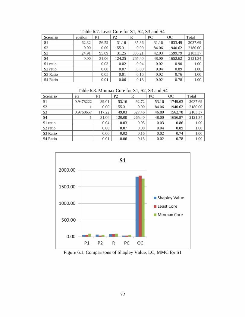
Table 6.7. Least Core for S1, S2, S3 and S4 Scenario epsilon P1 P2 R PC OC Total S1 62.32 56.52 31.16 85.36 31.16 1833.49 2037.69 S2 0.00 0.00 155.31 0.00 84.06 1940.62 2180.00 S3 24.91 95.09 31.25 335.21 42.03 1599.79 2103.37 S4 0.00 31.06 124.25 265.40 48.00 1652.62 2121.34 S1 ratio 0.03 0.02 0.04 0.02 0.90 1.00 S2 ratio 0.00 0.07 0.00 0.04 0.89 1.00 S3 Ratio 0.05 0.01 0.16 0.02 0.76 1.00 S4 Ratio 0.01 0.06 0.13 0.02 0.78 1.00

Table 6.8. Minmax Core for S1, S2, S3 and S4

Scenario eta P1 P2 R PC OC Total S1 0.9478222 89.01 53.16 92.72 53.16 1749.63 2037.69 S2 1 0.00 155.31 0.00 84.06 1940.62 2180.00 S3 0.9768657 117.22 49.03 327.46 46.89 1562.78 2103.37 S4 1 31.06 120.00 265.40 48.00 1656.87 2121.34 S1 ratio 0.04 0.03 0.05 0.03 0.86 1.00 S2 ratio 0.00 0.07 0.00 0.04 0.89 1.00 S3 Ratio 0.06 0.02 0.16 0.02 0.74 1.00 S4 Ratio 0.01 0.06 0.13 0.02 0.78 1.00

Figure 6.1. Comparisons of Shapley Value, LC, MMC for S1

72

Figure 6.2. Comparisons of Shapley Value, LC, MMC for S2

Figure 6.3. Comparisons of Shapley Value, LC, MMC for S3

73

Figure 6.4. Comparisons of Shapley Value, LC, MMC for S4

6.2. Result Interpretation

Although the Shapley value solution is not in the core for all scenarios and two scenarios

actually have an empty core, a close examination at the results and comparison of the scenario

differences could reveal the relative market power of those players, their interacting relationships,

and the reasons why the grand coalition is unstable.

In the Base Scenario (S1), the OC ships all containers via Terminal 1 and the railroad

(West Coast route). Of the total $126,784,000 (1981*64,000) coalition profit, the OC gets 89%,

the railroad gets 4%, the two terminals each get 3%, and the Canal gets 2%. Although OC ships

zero containers to P2 and the Panama Canal in S1 (See Table B1), the Shapley value suggests

that P2 and the Panama Canal still get positive profit allocations. Terminal 2 gets a total of

$3,989,120 (62.33*64,000) and the Panama Canal gets $2,275,840 (35.56*64,000). These profit

allocations are not a container handling revenue to the two players; instead, they are rewards to

74

them for their willingness to cooperate. The total profit gained by OC, P1, and the railroad has to

be shared with P2 and the Panama Canal, otherwise the OC may not ship via the WCR as in

Model 0, Model 1, etc. Apparently, this allocation is hard to accept by the other players. As the

core theory applies, the grand coalition in S1 is unstable. Some players would defect to a

different coalition solution. In the next chapter, two small coalitions will be analyzed and

compared to the grand coalition.

In the second scenario after the Panama Canal is expanded, the OC ships all containers

via Terminal 2 and the Panama Canal. The total coalition profit increases, so does the profit

share of the OC, P2, and PC. On the other hand, P1 and R get zero allocation. In S2, the grand

coalition has an un-empty core, and the Shapley value is in the core.

Comparing S1 and S2 (Figure 6.5), the relative market powers of the Canal and the port

on the East Coast (PC and P2) both increase after the Canal expansion is completed while the

powers of the WCR players (P1 and R) both decrease. The OC’s Shapley value also increases

after the expansion, but in a smaller magnitude than the PC and P1.

Figure 6.5. Panama Canal Expansion Impact S1 vs. S2

75

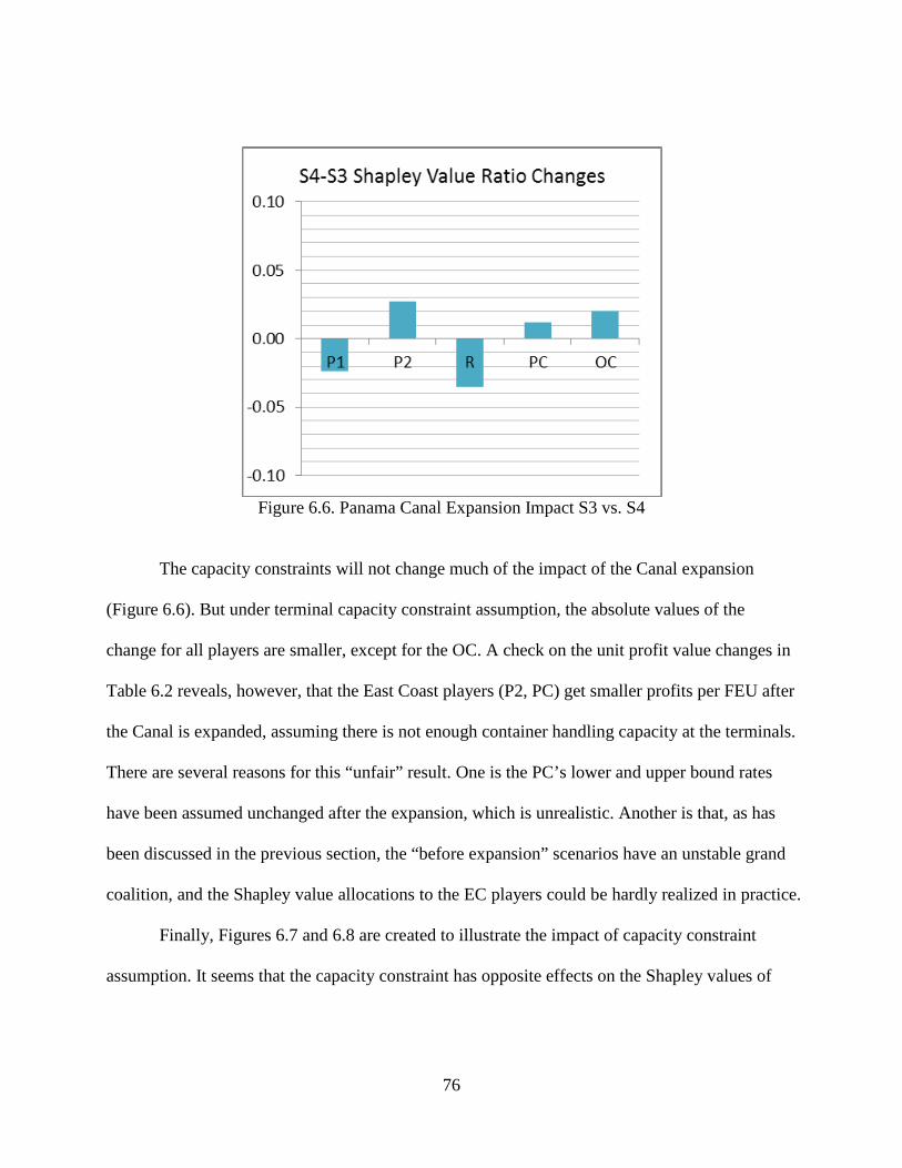
Figure 6.6. Panama Canal Expansion Impact S3 vs. S4

The capacity constraints will not change much of the impact of the Canal expansion

(Figure 6.6). But under terminal capacity constraint assumption, the absolute values of the

change for all players are smaller, except for the OC. A check on the unit profit value changes in

Table 6.2 reveals, however, that the East Coast players (P2, PC) get smaller profits per FEU after

the Canal is expanded, assuming there is not enough container handling capacity at the terminals.

There are several reasons for this “unfair” result. One is the PC’s lower and upper bound rates

have been assumed unchanged after the expansion, which is unrealistic. Another is that, as has

been discussed in the previous section, the “before expansion” scenarios have an unstable grand

coalition, and the Shapley value allocations to the EC players could be hardly realized in practice.

Finally, Figures 6.7 and 6.8 are created to illustrate the impact of capacity constraint

assumption. It seems that the capacity constraint has opposite effects on the Shapley values of

76

the OC and the railroad. When both terminals do have not enough resources to handle all

shipments, the OC loses profits while the railroad gains more.

Figure 6.7. Terminal Capacity Constraint Impact S1 vs. S3

Figure 6.8. Terminal Capacity Constraint Impact S2 vs. S4

77

Both LC and MMC results prove that the core is empty for scenarios S1 and S3 (ε > 0

and η < 1), while the core exists for S2 and S4 (ε <= 0 and η >= 1). An empty core indicates the

grand coalition is not stable, in the sense that there is no allocation solution that is not dominated

by other solutions, so that at least one player will defect to a different coalition, causing the

grand coalition to deform. In this case study, the ocean carrier is the dominant player and has two

route choices, causing the competition between the two routes unavoidable. Actually, a close

look at the S2 results reveals the reason that they could form a stable grand coalition in S2 is

because the OC always chooses the ECR no matter what kind of coalition is formed, and all

allocation methods (Shapley Value, LC, MMC) assign zero profits to the WCR players. Later it

is found that by changing some parameter values the results could change easily. Overall, the

grand coalition of the five players is very unstable.

6.3. Sensitivity Analysis

This section presents a sensitivity analysis on some model parameter values, and

discusses their impacts on the roles of the players in the container shipping market. The analysis

is based on the base scenario S1.The first parameter to be analyzed is the inventory cost

difference. In the model, the inventory cost is not directly included in the OC’s cost function,

because it is a cost to shippers. The shippers with higher valued goods are willing to pay more in

order to get quicker delivery. The shippers’ perceptions of delivery speed are reflected by the

OC’s charging rates. In order to charge more, the OC chooses a quicker route (WCR). The

difference between the two charging rates (R1 for WCR vs. R2 for ECR) is the average unit

inventory cost difference between the two routes.

78

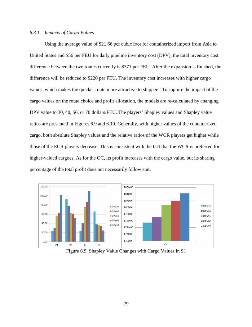
6.3.1. Impacts of Cargo Values

Using the average value of $21.66 per cubic foot for containerized import from Asia to

United States and $56 per FEU for daily pipeline inventory cost (DPV), the total inventory cost

difference between the two routes currently is $371 per FEU. After the expansion is finished, the

difference will be reduced to $220 per FEU. The inventory cost increases with higher cargo

values, which makes the quicker route more attractive to shippers. To capture the impact of the

cargo values on the route choice and profit allocation, the models are re-calculated by changing

DPV value to 30, 40, 56, or 70 dollars/FEU. The players’ Shapley values and Shapley value

ratios are presented in Figures 6.9 and 6.10. Generally, with higher values of the containerized

cargo, both absolute Shapley values and the relative ratios of the WCR players get higher while

those of the ECR players decrease. This is consistent with the fact that the WCR is preferred for

higher-valued cargoes. As for the OC, its profit increases with the cargo value, but its sharing

percentage of the total profit does not necessarily follow suit.

Figure 6.9. Shapley Value Changes with Cargo Values in S1

79

Figure 6.10. Shapley Value Ratio Changes with Cargo Values in S1

6.3.2. Impacts of Charging Rates

The lower and upper bounds of charging rates by the Panama Canal and the railroad are

studied in the same way by changing 10% from the base case. The lower bound of the rate is the

player’s cost of handling one unit of container, or the lowest rate the player is willing to accept to

handle one unit of container. The upper bound is the highest rate the player could charge under

non-cooperative assumption. The results are shown in Figure 6.11 to Figure 6.17.

When the railroad cost decreases, the absolute Shapley value and the ratio of the value for

the railroad increase while those values and ratios for P2 and PC decrease (Figure 6.11 and

Figure 6.12). The OC seems to get higher profit with reduced railroad cost, but its share of the

total profit actually gets smaller. Terminal 1’s shared profit first increases then decreases, which

is probably because of the two-sided effect of railroad cost. When the railroad cost is reduced,

the WCR benefits as a group, but the relative power of Terminal 1 compared with the railroad

also gets weaker. So when the railroad cost decreases to a certain value, the benefits gained by

P1 is less significant than the lost power to the railroad.

80

The railroad rate upper bound has almost no impact until it is lowered to 50% of the

original base case value (Figure 6.13). The railroad and the EC players get smaller profits, while

the OC and P1 get more profits. The ratios of the sharing follow the same pattern (Figure 6.14).

Figure 6.11. Shapley Value Changes with Railroad Rate Lower Bound in S1

Figure 6.12. Shapley Value Ratios Changes with Railroad Rate Lower Bound in S1

Figure 6.13. Shapley Value Changes with Railroad Rate Upper Bound in S1

81

Figure 6.14. Shapley Value Ratio Changes with Railroad Rate Upper Bound in S1

As for the Canal charging rate, the effect of changing lower and upper bound is very

different from the railroad. The ECR players’ Shapley values increase while the WCR players

and the OC’s profits decrease with the Canal’s cost decrease initially. However, when the lower

bound of the Canal rate further decreases to below 50% of the base-case assumption value

($160/FEU), the railroad’s profit starts to increase (Figure 6.15). The ratio changes follow the

same pattern (Figure 6.16).

Figure 6.15. Shapley Value Changes with Panama Canal Rate Lower Bound in S1

82

Figure 6.16. Shapley Value Ratio Changes with Panama Canal Rate Lower Bound in S1

When the Canal rate’s upper bound increases from 80% to 130% of base case assumption,

the Shapley values of railroad and the Canal both increase gradually; the OC’s Shapley value

decreases gradually; and the two terminals have no change (Figure 6.17). The ratio changes

follow exactly the same pattern (Figure 6.18). In the end, the OC’s charging rate is also analyzed.

Figure 6.19 clearly shows the OC’s rate only has impact on its own profit.

Figure 6.17. Shapley Value Changes with Panama Canal Rate Upper Bound in S1

83

Figure 6.18. Shapley Value Ratio Changes with Panama Canal Rate Upper Bound in S1

Figure 6.19. Shapley Value Changes with OC Rates in S1

6.3.3. Impacts of Capacity Constraint Assumption

In the end, the assumption of capacity constraint at the terminals is also analyzed by

varying the capacity level at the terminals. Assuming each terminal could handle 90% or 70% of

total shipment volume of the OC, the Shapley value ratios are compared with the original values

with 80% of capacity constraints. Figure 6.20 and Figure 6.21 show how the Shapley values and

Shapley value ratios change for each player when the capacity at the terminals changes. Again,

84

the capacity constraints clearly have positive impact on the railroad market power and negative

impact on the OC. For the other players, the impact is not linear.

Figure 6.20. Shapley Value Changes with Terminal Capacity Constraints

Figure 6.21. Shapley Value Ratio Changes with Terminal Capacity Constraints

6.4. Conclusions of Case Study

Four scenarios are conducted, and the model results indicate that if the grand coalition of

the five players is to form, the OC will ship all or most (depending on if there is enough capacity)

via the WCR before the Canal expansion. After the expansion is finished and both routes are

served by the 8,000-TEU vessel, the OC will prefer the all-waterway route via the Panama Canal

directly to the East Coast because of the higher profit.

85

When there is capacity constraint at the port terminals, the railroad gains more power

while the OC loses profit due to the constraints. Even assuming that both terminals could handle

the same amount of containers, the capacity constraint impact on the two terminals is not clear.

The Panama Canal’s impact on the relative power of the players is much more direct. The EC

benefits mostly, with OC’s profits increasing at a smaller degree, while the WC players lose

power due to the increasing power of their competitors.

The sensitivity analysis of some parameters in Scenario1 shows that the Shapley values

and value ratios of the five players are very sensitive to most parameter values. Although some

changes are very easy to expect, some are not very straightforward. Even with only five players

and two route choices, the interacting relationships are so complicated that the game results are

hard to predict without the help of model calculation.

Some general findings could still be drawn from the analysis of Scenario 1. If a player

could reduce its lower-bound rate (cost), that helps it gain more power in the coalition and get a

higher profit allocation. The impacts on other players are not very obvious. Although the OC’s

relative ratio decreases with reduced rail cost because it loses power to railroad, its absolute

profit improves. On the other hand, both the profit value and the portion of the OC get worse

when the Canal’s cost decreases. Regarding the different impacts of railroad cost and Canal cost

on the OC, one explanation is that in Scenario 1 the OC ships through WCR. Thus, lowering the

railway cost helps the coalition overall as well as the OC. Lowering the Canal cost, on the other

hand, does not save the grand coalition extra cost.

Another pattern of the cost impact is that the same route players’ profits change in the

same direction while different-route players’ profits change in the opposite direction. However,

this is only for the case with only two routes. When a player is involved in more than one route,

86

it is hard to define its partners or competitors. For this case study, if a transportation operator

could reduce its cost, it helps increase itself and its partner’s market power. Depending on if it

handles any containers for the OC, the cost reduction may or may not help the OC’s profit.

The highest possible rate the player could charge generally reflects its relative market

power. It works as a threat to the OC in that the OC has to pay a certain price level if no

cooperation happens. But it also increases its competitors’ profit or does not benefit itself at all,

as the railroad and the canal rate analyses show.

When the average cargo value of the container increases, the inventory cost difference

between the two routes also increases. This makes the WCR a more profitable choice for the OC,

and the competitive powers of the WCR players generally increase.

Most of the findings are consistent with real world practice and expectations. Some

results that are tricky to explain further prove that the shipping market is complicated and many

factors are making an effect at the same time. The cooperative game solutions offer a measurable

tool to understand interactive relationships in the ocean shipping industry, to compare the

relative powers of players, and to make predictions of market equilibrium.

The Least core (LC) and Minmax core (MMC) are calculated; and they produce very

similar results with the Shapley value. The advantages of LC and MMC are that they are much

easier to compute and they also seek a fairness solution. Of the four scenarios, S1 and S3, which

assume the current status of unfinished Panama-Canal-expansion, both have an empty core. By

changing some parameter values, the results could change easily. Overall, the grand coalition of

the five players is very unstable. The main reason is because, essentially, with only one ocean

carrier, the competition between the two routes is unavoidable. In the next chapter, two

following games are created supposing the grand coalition does not form.

87

7. FOLLOWING GAMES

7.1. West Coast Coalition and East Coast Coalition

As concluded in Chapter 6, the grand coalition of the five players is unstable because of

the competitive nature between the two routes. In this chapter, two separate possible coalitions

are derived and tested: the West Coast coalition (WCC) {OC, P1, R} and the East Coast

coalition (ECC) {OC, P2, PC}. Assuming the grand coalition could not form, the OC either

cooperates with P1 and R, or cooperates with P2 and PC. Only S1 and S2 are used for illustration.

The model results are given in Appendix C Table C1, C2, C3, and C4. The Shapley values are

presented below in Tables 7.1 and 7.2.

Table 7.1. Shapley Values and Value Ratios for West Coast Coalition {OC, P1, R} P1 R OC Total profit S1: West 152.656 1,327.000 558.031 2,037.687 S2: West 152.656 1,327.000 407.031 1,886.687 S1 Ratio: West 0.075 0.651 0.274 1.000 S2 Ratio: West 0.081 0.703 0.216 1.000

Table 7.2. Shapley Values and Value Ratios for East Coast Coalition {OC, P2, PC} P2 PC OC Total profit S1: East 153.125 72.813 1732.187 1958.125 S2: East 152.552 72.083 1955.208 2179.844 S1 Ratio: East 0.078 0.037 0.885 1.000 S2 Ratio: East 0.070 0.033 0.897 1.000

Similarly, as in Chapter 6, all values are divided by 64,000 for the purpose of easier

presenting and interpreting. For the small coalitions, the Shapley value could be directly

interpreted as a unit profit per FEU for every player. Tables 7.3 to 7.6 prove that all the Shapley

value solutions are in the core (One small negative value in Table 7.6 is a rounding error.) Both

coalitions are stable since the core exists. Apparently the ECC is preferred by the OC, because it

allocates higher profits for the OC. So the ECC will be studied in detail in this chapter.

88

Table 7.3. West Coast Coalition Values in S1 Players v(S) OC P1 R sum(yi) sum(yi) -v(S) OC 555.38 558.03

558.03 2.66

OC P1 710.69 558.03 152.66

710.69 0.00 OC R 1882.38 558.03

1327.00 1885.03 2.66

OC P1 R 2037.69 558.03 152.66 1327.00 2037.69 0.00 P1 R 1477.00

152.66 1327.00 1479.66 2.66

R 1327.00

1327.00 1327.00 0.00 P1 150.00

152.66

152.66 2.66

Table 7.4. West Coast Coalition Values in S2 Players v(S) OC P1 R sum(yi) sum(yi) -v(S) OC 404.38 407.03

407.03 2.66

OC P1 559.69 407.03 152.66

559.69 0.00 OC R 1731.38 407.03

1327.00 1734.03 2.66

OC P1 R 1886.69 407.03 152.66 1327.00 1886.69 0.00 P1 R 1477.00

152.66 1327.00 1479.66 2.66

R 1327.00

1327.00 1327.00 0.00 P1 150.00

152.66

152.66 2.66

Table 7.5. East Coast Coalition Values in S1 Players v(S) OC P2 PC sum(yi) sum(yi) -v(S) OC 1716.25 1732.19

1732.19 15.94

OC P2 1872.50 1732.19 153.13

1885.31 12.81 OC PC 1801.88 1732.19

72.81 1805.00 3.13

OC P2 PC 1958.13 1732.19 153.13 72.81 1958.13 0.00 P2 PC 210.00

153.13 72.81 225.94 15.94

PC 60.00

72.81 72.81 12.81 P2 150.00

153.13

153.13 3.13

89

Table 7.6. East Coast Coalition Values in S2 Players v(S) OC P2 PC sum(yi) sum(yi) -v(S) OC 1940.63 1955.21

1955.21 14.58

OC P2 2095.63 1955.21 152.55

2107.76 12.14 OC PC 2024.69 1955.21

72.08 2027.29 2.60

OC P2 PC 2180.00 1955.21 152.55 72.08 2179.84 -0.16 P2 PC 210.00

152.55 72.08 224.64 14.64

PC 60.00

72.08 72.08 12.08 P2 150.00

152.55

152.55 2.55

The ECC gets slightly lower total profit than the grand coalition. In S1, both P2 and PC

get better results in the ECC than in the grand coalition, although the OC actually gets less. In S2,

all the players in ECC get almost the same as the result in the grand coalition game.

Every player in the small coalition gains extra profit compared with playing as singletons. For

example, as shown in Table 7.5, the OC gains an extra $15.94 per FEU, the PC gains an extra

$12.81 per FEU, and P2 gains an extra $3.13 per FEU, compared with playing individually

against the rest of players. The total extra profit gained by all three players in the ECC is $31.88

per FEU. To prove that this amount is the exact total gain of this coalition due to the cooperating

benefit, the coalition value is estimated again assuming there is no benefit of cooperating, i.e., no

transit time saving. Results are pasted in Appendix C Table C5. The results are compared in

Table 7.7 below. The cooperation of the three players adds a total of $31.88 per FEU to the

coalition profit, assuming transit time is saved 0.5 days at the terminal and at the Canal. This

benefit gained by the coalition is allocated to each player based on Shapley value calculation

rules.

Table 7.7. Shapley Value Changes Due to Cooperation of ECC in S1 P2 PC OC Total profit S1:Cooperation Benefit 153.125 72.813 1732.187 1958.125 S1: No-Cooperation Benefit 150.000 60.000 1716.250 1926.250 S1 Changes 3.125 12.813 15.938 31.875

90

The Shapley Value is by far the most popular allocation method in cooperative game

theory. Of the total profit of $1,958.125 for the coalition in Scenario 1, P2 gets a profit of

$153.125, the PC gets a profit of $72.813, and the OC gets the rest. Considering the cost of $150

per FEU for P2 and $160 per FEU for PC, that means the OC would pay $303.125 per FEU to P2

and $232.813 per FEU to PC. Note the highest rates charged by the two players under non-

cooperative assumption are $300 and $220 per FEU, respectively. The collaboration between the

three players saves transit time and operating cost for the OC. The cooperative game theory

proves that when the three players negotiate prices, the terminal and the Canal actually get more

than the amount they would charge if no cooperation exists, but the OC still benefits because the

cost saved from cooperating is more than the extra amount it pays to other players. How much of

the benefit the OC has to return to the other two players depends on the relative market powers

of the three players. In order to have a stable coalition, the division of total benefits has to be un-

dominated by any other allocation method. When the Shapley value is in the core, the allocation

method is un-dominated and stable.

Comparing the before and after expansion scenario results (S1 vs. S2), the benefit of

using a larger vessel is mostly gained by the OC. The Canal, on the other hand, has almost no

change of profit. The reason for this “unfair” result is partly because in Scenario 2, the lower and

upper bound of the Canal rate is assumed as unchanged. In reality, it is expected the Canal

should increase both its cost and maximum charging rates. In the next section, sensitivity

analysis on the Canal’s cost and rate are conducted to analyze how those values will affect the

Canal’s role in the coalition.

91

Least core and Minmax core are also calculated (Table 7.8, 7.9). Similarly, like the grand

coalition, both methods produce very similar results to the Shapley value solutions for the ECC

(Figure 7.1, 7.2). Clearly, the core exists for ECC in both S1 and S2.

Table 7.8. Least Core for ECC in S1 Scenario epsilon P2 PC OC Total profit S1 -3.125 153.125 82.500 1722.500 1958.125 S2 -2.656 152.656 81.719 1945.625 2180.000

Table 7.9. Minmax Core for ECC in S1 Scenario eta P2 PC OC Total profit S1 1.003 150.480 79.629 1728.016 1958.125 S2 1.002 150.366 79.256 1950.378 2180.000

Figure 7.1. Comparisons of Shapley Value, LC, MMC for ECC in S1

92

Figure 7.2. Comparisons of Shapley Value, LC, MMC for ECC in S2

7.2. Sensitivity Analysis for the Following Games

Sensitivity analysis on some parameter values is conducted for the ECC. The cost of

Terminal 2 and the Canal are analyzed first. Decreasing the Canal cost (CRL) by $16 per FEU

will increase its Shapley value by exactly $16 per FEU (Table 7.10). Similarly, decreasing

Terminal 2’s cost (PRL2) by $15 per FEU will increase its allocated profit by $15 per FEU

(Table 7.11). The cost reduction has benefit to the whole coalition, but all the benefit is allocated

to the player itself.

Table 7.10. Shapley Value Changes with PC Lower Bound Rate in S1 P2 PC OC CRL0.5 153 153 1732 CRL0.6 153 137 1732 CRL0.7 153 121 1732 CRL0.8 153 105 1732 CRL0.9 153 89 1732 Base 153 73 1732

93

Table 7.11. Shapley Value Changes with P2 Lower Bound Rate in S1 P2 PC OC PRL0.5 228 73 1732 PRL0.6 213 73 1732 PRL0.7 198 73 1732 PRL0.8 183 73 1732 PRL0.9 168 73 1732 Base 153 73 1732

As shown in Table 7.12, increasing the Canal rate upper bound (CRU) by 1% ($22 per

FEU) will increase its Shapley value by 1% ($22 per FEU) and decrease the OC’s value by the

same amount. Terminal 2 is not impacted. The same impact of changing the terminal upper

bound rate (PRU2) happens (Table 7.13). That is because the rate is a side payment inside the

coalition, and has no impact on the coalition’s value.

Table 7.12. Shapley Value and Ratio Changes with PC Upper Bound Rate in S1 P2 PC OC CRU0.8 153.13 28.81 1776.19 CRU0.9 153.13 50.81 1754.19 Base 153.13 72.81 1732.19 CRU1.1 153.13 94.81 1710.19 CRU1.2 153.13 116.81 1688.19 CRU1.3 153.13 138.81 1666.19 CRU0.8 Ratio 0.08 0.01 0.91 CRU0.9 Ratio 0.08 0.03 0.90 Base Ratio 0.08 0.04 0.88 CRU1.1 Ratio 0.08 0.05 0.87 CRU1.2 Ratio 0.08 0.06 0.86 CRU1.3 Ratio 0.08 0.07 0.85

94

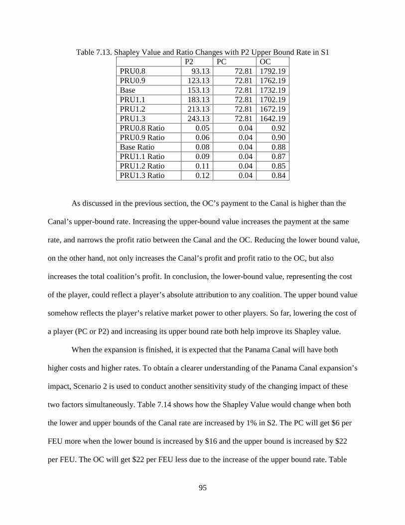
Table 7.13. Shapley Value and Ratio Changes with P2 Upper Bound Rate in S1 P2 PC OC PRU0.8 93.13 72.81 1792.19 PRU0.9 123.13 72.81 1762.19 Base 153.13 72.81 1732.19 PRU1.1 183.13 72.81 1702.19 PRU1.2 213.13 72.81 1672.19 PRU1.3 243.13 72.81 1642.19 PRU0.8 Ratio 0.05 0.04 0.92 PRU0.9 Ratio 0.06 0.04 0.90 Base Ratio 0.08 0.04 0.88 PRU1.1 Ratio 0.09 0.04 0.87 PRU1.2 Ratio 0.11 0.04 0.85 PRU1.3 Ratio 0.12 0.04 0.84

As discussed in the previous section, the OC’s payment to the Canal is higher than the

Canal’s upper-bound rate. Increasing the upper-bound value increases the payment at the same

rate, and narrows the profit ratio between the Canal and the OC. Reducing the lower bound value,

on the other hand, not only increases the Canal’s profit and profit ratio to the OC, but also

increases the total coalition’s profit. In conclusion, the lower-bound value, representing the cost

of the player, could reflect a player’s absolute attribution to any coalition. The upper bound value

somehow reflects the player’s relative market power to other players. So far, lowering the cost of

a player (PC or P2) and increasing its upper bound rate both help improve its Shapley value.

When the expansion is finished, it is expected that the Panama Canal will have both

higher costs and higher rates. To obtain a clearer understanding of the Panama Canal expansion’s

impact, Scenario 2 is used to conduct another sensitivity study of the changing impact of these

two factors simultaneously. Table 7.14 shows how the Shapley Value would change when both

the lower and upper bounds of the Canal rate are increased by 1% in S2. The PC will get $6 per

FEU more when the lower bound is increased by $16 and the upper bound is increased by $22

per FEU. The OC will get $22 per FEU less due to the increase of the upper bound rate. Table

95

7.15 shows how the Shapley Value would change when both the lower and upper bounds of

Terminal 2 rate are increased by 1% in S2. P1 will get $15 per FEU more when the lower bound

is increased by $15 and the upper bound is increased by $30 per FEU. The OC will get $30 less

due to the increase of the upper bound rate.

Table 7.14. Shapley Value and Ratio Changes with CRL and CRU in S2 P2 PC OC CRLCRU1.3 152.55 90.08 1889.21 CRLCRU1.2 152.55 84.08 1911.21 CRUCRL1.1 152.55 78.08 1933.21 Base (S2) 152.55 72.08 1955.21 CRU1.3 Ratio 0.072 0.042 0.886 CRU1.2 Ratio 0.071 0.039 0.890 CRU1.1 Ratio 0.071 0.036 0.893 Base Ratio 0.070 0.033 0.897

Table 7.15. Shapley Value and Ratio Changes with PRL and PRU in S2 P2 PC OC PRLPRU1.3 197.55 72.08 1865.21 PRLPRU1.2 182.55 72.08 1895.21 PRLPRU1.1 167.55 72.08 1925.21 Base (S2) 152.55 72.08 1955.21 CRU1.3 Ratio 0.093 0.034 0.874 CRU1.2 Ratio 0.085 0.034 0.882 CRU1.1 Ratio 0.077 0.033 0.889 Base Ratio 0.070 0.033 0.897

It seems the impacts of lower and upper bound rates are linear on the players’ Shapley

values and are uncorrelated in the ECC. If the Canal operator could increase its rate more than

the increased cost due to the expansion, the PC will have improved profit allocation in the ECC

after the expansion is finished.

7.3. Conclusions of Following Games

Two small coalitions are analyzed and both have stable Shapley value solutions.

Compared with the two small coalitions, the grand coalition has the highest total profit and offers

96

the OC the highest profit allocation. However, all the other players get better profits in their

small coalition than in the grand coalition. Comparing the two small coalitions, the OC prefers

the East Coast Coalition {OC, P2, PC} because it offers a higher profit than the West Coast

Coalition {OC, P1, R}.

Using the ECC to illustrate, the Shapley values allocate the benefits of cooperation to

each player in the coalition {OC, P2, PC}. The allocation is efficient because the sum of benefit

to each player is equal to the total benefit of the coalition. Because the Shapley value solution for

the small coalitions is in the core, the allocation is also stable. LC and MMC provide very similar

results to the Shapley Value.

Sensitivity analysis is conducted. A player’s cost reduction has benefit to the whole

coalition, but all the benefit is allocated to the player itself. The cost in some way reflects a

player’s absolute attribution to a coalition. On the other hand, the player’s upper bound rate

affects its relative market power to the OC. It has no impact on the coalition’s value, and only

changes the allocation difference between the player and the OC. Simultaneous changes of the

PC’s upper and lower bound rates are tested, as well as P2’s upper and lower bound rates. It

seems the impacts of lower and upper bound rates are linear and are not correlated in the small

coalition.

The cost and rate changes’ impact on players’ profit values and ratios is very different

from the grand coalition analysis in Chapter 6. The grand coalition has more complicated

competition-cooperation relationships within its members. In contrast, the ECC has only three

players and no competition exists among them. When more players are involved and more

shipping chains and routes are available, the market becomes more complex and prediction of

corporation/competition results could not be easily made intuitively. Using game theory to

97

analyze the situation becomes more necessary for those situations. And, as shown by this case

study, the Shapley value, LC, and MMC all have successfully analyzed the interacting

relationship.

The last conclusion regards the Panama Canal expansion effect. In the ECC, the PC will

not get a better profit if holding the Canal rate’s upper bound and lower bound constant. If, as

expected, the Panama Canal operator will increase its rate more than the increased cost after the

expansion, the PC will have improved profit allocation in the ECC after the expansion is finished.

98

8. SUMMARY AND CONCLUSIONS

8.1. Summary of the Problem

The container shipping market is confronted with many challenges and has caught wide

attention of many researchers. In addition to uncertainties and congestion problems, the

complicated interacting relationships between the various agents are continuously changing and

have important and direct impact on the shipment routes, volume, and prices. Different

stakeholders along the shipment chain have different, very often conflicting, economic goals and

may have cooperation or competition relationships. Their different market power impacts the

negotiation process and how the profits/cost savings are divided.

One type of existing approaches to cargo spatial distribution problems uses optimization

modeling and usually ignores the impact of stakeholders interactions. Another type either

implicitly models the competition equilibrium of carriers and shippers, like Network Equilibrium

Models, or explicity evaluates some types of non-cooperative strategies or cooperative solutions

in the system. It is noticed that more comprehensive applications of non-cooperative game theory

and some types of cooperative game approaches on the freight network planning problems began

to merge. Some of those also used multi-level programming programs to examine the hierarchy

relationships. But the applications are rare and apparently at an early stage.

In this dissertation, the cooperative game theory is utilized to solve the U.S. containerized

import shipment optimization problem, and to investigate the relationships between the players.

Bi-level optimization models are built to capture the hierarchy structure of the ocean shipping

industry. Different types of coalitions and competition-cooperation schemes for the main players

are assumed and solved using different bi-level models. The model results are input into

cooperative game solutions. The Shapley value, the core, Least core, and Minmax core are

99

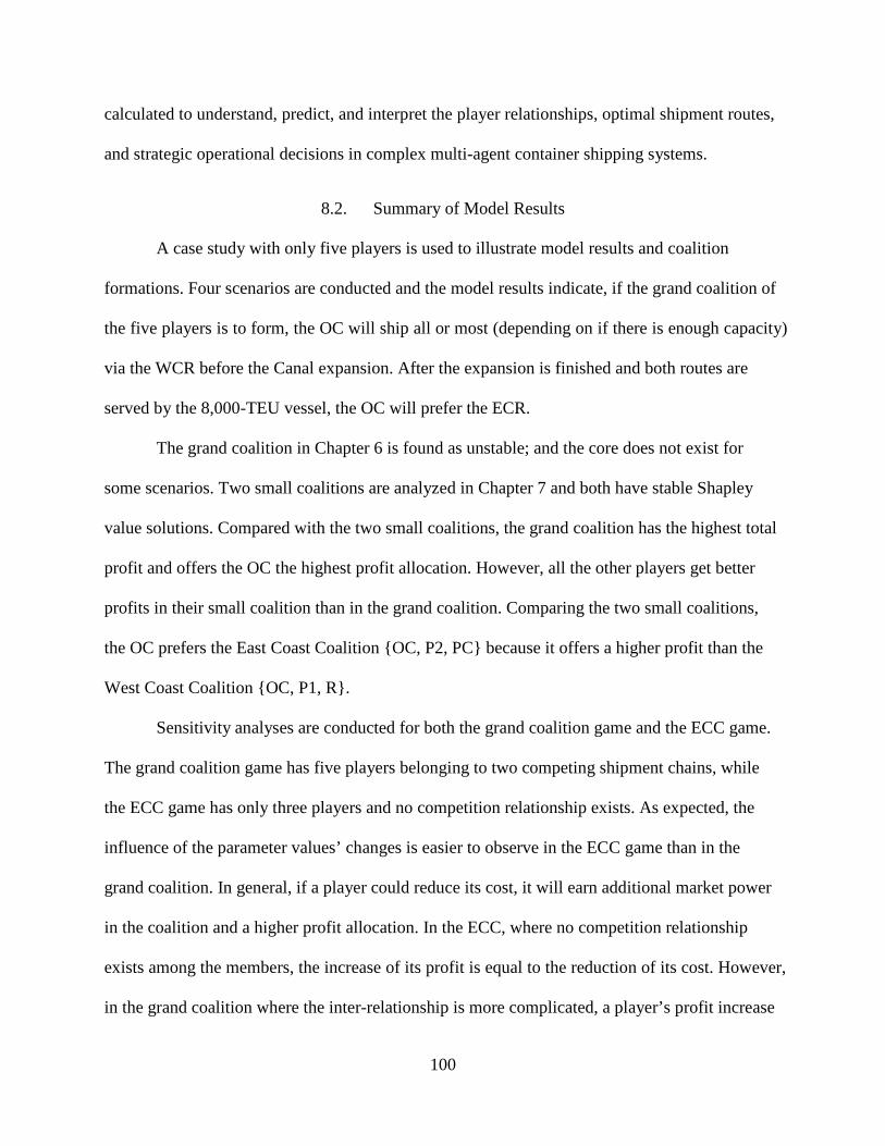
calculated to understand, predict, and interpret the player relationships, optimal shipment routes,

and strategic operational decisions in complex multi-agent container shipping systems.

8.2. Summary of Model Results

A case study with only five players is used to illustrate model results and coalition

formations. Four scenarios are conducted and the model results indicate, if the grand coalition of

the five players is to form, the OC will ship all or most (depending on if there is enough capacity)

via the WCR before the Canal expansion. After the expansion is finished and both routes are

served by the 8,000-TEU vessel, the OC will prefer the ECR.

The grand coalition in Chapter 6 is found as unstable; and the core does not exist for

some scenarios. Two small coalitions are analyzed in Chapter 7 and both have stable Shapley

value solutions. Compared with the two small coalitions, the grand coalition has the highest total

profit and offers the OC the highest profit allocation. However, all the other players get better

profits in their small coalition than in the grand coalition. Comparing the two small coalitions,

the OC prefers the East Coast Coalition {OC, P2, PC} because it offers a higher profit than the

West Coast Coalition {OC, P1, R}.

Sensitivity analyses are conducted for both the grand coalition game and the ECC game.

The grand coalition game has five players belonging to two competing shipment chains, while

the ECC game has only three players and no competition relationship exists. As expected, the

influence of the parameter values’ changes is easier to observe in the ECC game than in the

grand coalition. In general, if a player could reduce its cost, it will earn additional market power

in the coalition and a higher profit allocation. In the ECC, where no competition relationship

exists among the members, the increase of its profit is equal to the reduction of its cost. However,

in the grand coalition where the inter-relationship is more complicated, a player’s profit increase

100

is less than its cost reduction; and some benefit is allocated to the OC or other players. On the

other hand, a player’s upper bound rate is the highest rate that it could charge in a non-

cooperative market, and affects its relative market power in relation to its coalition members.

Sensitivity analysis on the average cargo value in grand coalition proves that the quicker

route is preferred for higher-valued cargoes, as more pipeline inventory cost is saved, ceteris

paribus. In the grand coalition, the ECR players (P2 and PC) both benefit from the Canal

expansion in terms of both Shapley value and unit profit even when the Canal’s rate range is

assumed unchanged. However, when there is capacity constraint at the East Coast terminal, EC

players’ Shapley values increase due to the expansion, but their unit profits actually decrease. In

the ECC, the PC will not get a better profit if holding the Canal rate’s upper bound and lower

bound constant. All the benefit to the coalition due to the Panama Canal expansion is gained by

the OC. If, as expected, the Panama Canal operator will increase its rate more than the increased

cost after the expansion, the PC will have improved profit allocation in the ECC after the

expansion is finished.

8.3. Implications

The different solution results of the 15 different bi-level models are a clear indication that,

with different cooperation schemes, the OC will have different route choices and rate payments

to other players. Ignoring the relationships of multiple entities fails to understand the real

container shipping market.

The finding that the grand coalition for the case study is very unstable is mainly because

there are two competing routes for one OC. That will not be necessarily true if more players are

added to the game. And actually, by changing some parameter values, the grand coalition for this

case study might have an un-empty core. Similarly, although the ECC is preferred by P2 and PC

101

for this case study, the result may change if the parameter values and number of players in the

game are changed. For each new case, the models have to be re-built and computed and solutions

have to be re-calculated.

Based on the case study, the Panama Canal’s expansion clearly has a positive impact on

the relative market power of the ECR and a negative impact on the WCR when there is no

capacity constraint problem. The Canal expansion has a two-sided impact on the OC in that it

may save vessel operating costs for the OC, and may also hurt the OC’s relative market power

and final profit allocation.

Most of the findings are consistent with real world practice and expectations. Some

results that are tricky to explain further prove that the shipping market is complicated and many

factors are having an effect at the same time. When many players are involved in the market,

player relationships will become more complicated, and the corporation and competition results

could hardly be predicted intuitively. The cooperative game solutions offer a measurable tool to

understand the interactive relationships in the ocean shipping industry, to compare the relative

powers of players, and to make predictions of market equilibrium.

8.4. Contributions

The research contributes to the literature in a number of aspects.

1. Compared with studies that ignore player relationships, this dissertation incorporates four

types of players in the U.S. containerized import market to analyze the optimal container

shipment problem using cooperative game theory approaches. In contrast to some studies

that focused on interactions of one or two types of players, the four types of players in

this study are from different levels of the shipment chain, and their relationships are

much more complicated than relationships among the same-level players. Different

102

solution approaches, including the core, Shapley value, Least core, and Minmax core, are

used. From the extensive literature review, there are almost no studies of this type.

2. The hierarchy structure between the OC and the other players is captured by Bi-level

Programming Problems (BLPP). In all, 16 bi-level models are built and calculated and 32

coalitions are analyzed for the case study. Following games are also added after the grand

coalition is considered unstable.

3. While the Panama Canal expansion has been discussed vastly by scholars, no studies

have quantitatively evaluated its impact on the container flow pattern or the market

power of the different stakeholders in the container shipping market. This study shows

that by comparing the before and after scenarios, the Panama Canal expansion’s impact

on the market could be directly investigated. By varying assumptions on terminal

capacity constraints and other parameter values, insights on how the players interact with

each other have also been gained.

8.5. Limitations, Challenges and Suggestions for Future Research

The five-player case study suffices for the purpose of demonstrating how the bi-level

models are built and computed, and how the cooperative game solutions are calculated and

interpreted for the U.S. container import market. But it is not sufficient to get a thorough picture

of the market status, or even predict future market equilibrium. Similarly, a complete

understanding of the Panama Canal’s expansion and capacity constraint impact could not be

obtained at this point.

In order to achieve that goal, more players need to be added to include nationwide

containerized-import shipments. However, to include just 10 major U.S. ports, two origins (Asia

and Europe), 48 contiguous states as the inland destinations, and five shipping companies, there

103

will be at least 10 port operators, four U.S. railroad operators (BNSF, CSX, NS, CN), one

trucking operator (assuming there is no competition among all trucking companies), two canal

operators (Panama Canal and Suez Canal), and five OCs. With 22 players, the total number of

possible coalitions will be 4,194,304 (222). For a simplier version with only five port operators,

one railroad operator, one trucking operator, two canal operators, and three ocean carriers, there

will still be 2,048 (211) coalition combinations. One solution to the large number of coalitions is

to eliminate some “unrealistic” coalitions in the beginning. For example, assume there is no

cooperation between the ports. When capacity constraints at some nodes or links are further

assumed, the problem will become more intricate. The number of mathematical models and the

complexity of each model will both rise dramatically. It is a challenge to model such a complex

system using cooperative game theory approach.

Fixed demand is assumed in the dissertation, and the shippers’ role is not considered. To

have a demand function instead of the fixed value, the shippers’ interaction with the OC could be

analyzed. But the model will become hard to solve and the global solution algorithm has to be

established. Trucking companies are not considred in the case study; and the demand destination

is purposely selected to be very near Terminal 2. If a more interior destination is used instead, an

inland carrier for the ECR has to be added, which will affect the power structure of the market.

Another important player that has been neglected in this study is the Suez Canal, due to

the time limitation. A shift in trade lanes is underway already as some big shipping companies

(e.g., Maersk Lines) are already transpassing via the Suez Canal instead of the Panama Canal for

the Asia to East Coast routes. As the Panama Canal expansion is not finished yet, carriers have

found that using large PostPanamax vessels on the Suez route to the East Coast is more

104

profitable than through the Panama Canal. Adding the Suez Canal as another player is expected

to change the power structure of the players, especially for the Panama Canal.

The Shapley value calculation is computatively extensive. As shown by this study, the

LC and MMC provide very similar results to the Shapley Value, and have the advantages of

much easier computation requirements and seeking fairness. For future research on a more

complicated game, these two could be used instead of the Shapley value.

105

REFERENCES

Adamidou, Evdokia A. , and Alain L. Kornhauser. 1993. "A Game Theoretic/Network

Equilibrium Solution Approach For The Railroad Freight Car Management Problem." Transportation Research Part B no. 27 (3):237-252.

Adler, Nicole. 2001. "Competition in a Deregulated Air Transportation Market." European Journal of Operational Research no. 129:337-345.

Al-Khayal, Faiz A., Reiner Horst, and Panos M. Pardalos. 1992. "Global Optimization of Concave Functions Subject to Quadratic Constraints: An Application in Nonlinear Bilevel Programming." Annals of Operations Research no. 34 (1):125-147.

Álvarez-SanJaime, Óscar, Pedro Cantos-Sánchez, Rafael Moner-Colonques, and José J. Sempere-Monerris. 2013. "Vertical Integration and Exclusivities in Maritime Freight Transport." Transportation Research Part E no. 51:50-61.

Anandalingam, G., and K. Nam. 1997. "Conflict and Cooperation in Designing International Telecommunication Networks." Journal of the Operational Research Society no. 48:600-611.

Army Corps of Engineers. 2007. USACE Aggregate Vessel Operating Cost Model. Maritime Strategies International, Ltd. and The Institute for Water Resources, US Army Corps of Engineers.

Arshinder, Arun Kanda, and S. G. Deshmukh. 2008. "Supply Chain Coordination: Perspectives, Empirical Studies And Research Directions." International Journal of Production Economics no. 115 (2):316-335.

Asgari, Nasrin, Reza Zanjirani Farahani, and Mark Goh. 2013. "Network Design Approach for Hub Ports-Shipping Companies Competition and Cooperation." Transportation Research Part A no. 48:1-18.

Audy, J. F., S. D’Amours, and L. M. Rousseau. 2011. "Cost Allocation in the Establishment of a Collaborative Transportation Agreement―An Application in the Furniture Industry." Journal of the Operational Research Society no. 62:960-970.

Aumann, R. J. 1959. "Acceptable Points in General Cooperative N-Person Games." In Contributions to the Theory of Games IV, edited by A.W. Tucker and R.D. Luce, 287-324. Princeton, NJ: Princeton University Press.

Aumann, R.J., and L.S. Shapley. 1974. Values of Non-Atomic Games. Princeton, NJ.: Princeton University Press.

106

Bahn, O., A. Haurie, S. Kypreos, and J.-P. Vial. 1998. "Advanced Mathematical Programming Modeling to Assess the Beneits of International CO2 Abatement Cooperation." Environmental Modeling and Assessment no. 3 (1/2):107-116.

Bard, Jonathan F. 1988. "Convex Two-Level Optimization." Mathematical Programming no. 40:15-27.

Bard, Jonathan F., and James Falk. 1982. "An Explicit Solution to the Multi-Level Programming Problem." Computers and Operations Research no. 9:77-100.

Bard, Jonathan F., and James T. Moore. 1990. "A Branch and Bound Algorithm for the Bilevel Programming Problem." SIAM Journal on Scientific and Statistical Computing no. 11 (2):281-292.

Bartholdi, John J. III, and Eda Kemahlioglu-Ziya. 2004. "Using Shapley Value To Allocate Saving in a Supply Chain." In Supply Chain Optimization, edited by Joseph Geunes and Panos M. Pardalos. Kluwer Optimization Series.

Bianco, Lucio, Massimiliano Caramia, and Stefano Giordani. 2009. "A Bilevel Flow Model for Hazmat Transportation Network Design." Transportation Research Part C no. 17:175-196.

Bloomberg L. P. 2013a. Data on Daily Hire Rates for Ocean Freight from Japan-South Korea to US-Can North Pacific 7/13/2005 to 8/1/2013. Retrieved September 3, 2013 from Bloomberg terminal.

Bloomberg L. P. 2013b. Data series on 380cst and MDO at Port of Los Angeles from 7/31/2000 to 7/29/2013. Retrived September 3, 2013 from Bloomberg terminal.

Bonney, Joseph. 2012. ILA, USMX Resume Contract Talks. http://www.joc.com/port-news/longshoreman-labor/ila-usmx-resume-contract-talks_20120628.html.

Bonney, Joseph. 2013. ILA, Employers Resume Local Bargaining. http://www.joc.com/port-news/longshoreman-labor/international-longshoremen%E2%80%99s-association/ila-employers-resume-local-bargaining_20130204.html.

Bracken, Jerome, and James T. McGill. 1973. "Mathematical Programs with Optimization Problems in the Constraints." Operations Research no. 21:37-44.

Bracken, Jerome, and James T. McGill. 1974. "Defense Applications of Mathematical Programs with Optimization Problems in the Constraints." Operations Research no. 22:1086-1096.

Bracken, Jerome, and James T. McGill. 1978. "Production and Marketing Decisions with Multiple Objectives in a Competitive Environment." Journal of Optimization Theory and Applications no. 24:449-458.

107

Brooks, Mary. 1993. "International Competitiveness-Assessing and Exploring Competitive Advantage by Ocean Container Carriers." Logistics and Transportation Review no. 29 (3):278-293.

Cachon, Gerard P., and Martin A. Lariviere. 1999. "Capacity Allocation Using Past Sales: When to Turn and Earn." Management Science no. 45:685-703.

Cachon, Gerard P., and Martin A. Lariviere. 2005. "Supply Chain Coordination with Revenue-Sharing Contracts: Strengths and Limitations." Management Science no. 51 (1):30-44.

Cachon, Gerard P., and Serguei Netessine. 2004. "Game Theory in Supply Chain Analysis." In Supply Chain Analysis in the eBusiness Era, edited by David Simchi-Levi, S. David Wu and Zuo-Jun Shen. Kluwer.

Candler, W., and R. Norton. 1977. Multilevel Programming, Technical Report 20. Washington D.C., USA: World Bank Development Research Center.

Castelli, Lorenzo, Giovanni Longo, Raffaele Pesenti, and Walter Ukovich. 2004. "Two-Player Noncooperative Games Over a Freight Transportation Network." Transportation Science no. 38 (2):149-159.

Chapman, Dan. 2012. Ports to Spend Big for Global Bounty. http://www.ajc.com/news/news/local/ports-to-spend-big-for-global-bounty/nQWWX/.

Chen, Rachel R., and Shuya Yin. 2010. "The Equivalence of Uniform and Shapley Value-Based Cost Allocations in a Specific Game." Operations Research Letters no. 38:539-544.

Colson, Benoît, Patrice Marcotte, and Gilles Savard. 2007. "An Overview of Bilevel Optimization." Annals Operations Research no. 153:235-256.

Cruijssen, Frans, Peter Borm, Hein Fleuren, and Herbert Hamers. 2010. "Supplier-Initiated Outsourcing: A Methodology to Exploit Synergy in Transportation." European Journal of Operational Research no. 207:763-774.

Drechsel, J., and A. Kimms. 2010. "Computing core Allocations Incooperative Games with an Application to Cooperative Procurement." International Journal of Production Economics no. 128:310-321.

Drechsel, J., and A. Kimms. 2011. "Cooperative Lot Sizing with Transshipments and Scarce Capacities: Solutions and Fair Cost Allocations." International Journal of Production Research no. 49 (9):2643-2668.

Edmunds, Thomas A., and Jonathan F. Bard. 1991. "Algorithms for Nonlinear Bilevel Mathematical Programs." IEEE Transactions on Systems, Man, and Cybernetics no. 21 (1):83-89.

108

Edmunds, Thomas A., and Jonathan F. Bard. 1992. "An Algorithm for the Mixed-Integer Nonlinear Bilevel Programming Problem." Annals of Operations Research no. 34:149-162.

Fan, Lei. 2010. Optimization Model and Risk Analysis for Global Supply Chain in Container Shipments: Imports to the United States. PhD Dissertation, Transportation and Logistics, North Dakota State University.

Fan, Lei, William Wilson, and Bruce Dahl. 2012. "Congestion, Port Expansion and Spatial Competition for Us Container Imports." Transportation Research Part E no. 48 (6):1121-1136.

Fan, Lei, William Wilson, and Denver Tolliver. 2010. "Optimal Network Flows for Containerized Imports to the United States." Transportation Research Part E no. 46 (5):735-749.

Fatima, Shaheen S., Michael Wooldridge, and Nicholas R. Jennings. 2008. "A Linear Approximation Method for the Shapley Value." Artificial Intelligence no. 172:1673-1699.

Filar, J. A., and P. S. Gaertner. 1997. "A Regional Allocation of World CO2 Emission Reductions." Mathematics and Computers in Simulation no. 43:269-275.

Ford, Eric W., Rebecca Wells, and Barbara Bailey. 2004. "Sustainable Network Advantages: A Game Theoretic Approach to Community-Based Health Care Coalitions." Health Care Management Review no. 29:159-169.

Fortuny-Amat, José, and Bruce McCarl. 1981. "A Representation and Economic Interpretation of a Two-Level Programming Problem." The Journal of the Operational Research Society no. 32 (9):783-792.

Franc, Pierre, and Martijin Van der Horst. 2010. "Understanding Hinterland Service Integration by Shipping Lines and Terminal Operators: A Theoretical And Empirical Analysis." Journal of Transport Geography no. 18 (4):557-566.

Frisk, M., M. Göthe-Lundgren, K. Jörnsten, and M. Rönnqvist. 2010. "Cost Allocation in Collaborative Forest Transportation." European Journal of Operational Research no. 205:448-458.

Fusillo, Michael. 2006. "Some Notes on Structure and Stability in Liner Shipping." Maritime Policy and Management no. 33 (5):463-475.

Gillies, D. B. 1959. Solutions to General Non-Zero-Sum Games.

Hackett, Ben. 2003. "National Dredging Needs Study of U.S. Ports and Harbors: Update 2000." DRI-WEFA.

109

Hansen, Pierre, Brigitte Jaumard, and Gilles Savard. 1992. "New Branch-and-Bound Rules for Linear Bilevel Programming." SIAM Journal of Scientific and Statistical Computing no. 13:1194-1217.

Harker, Patrick T., and Terry L. Friesz. 1986a. "Prediction of Intercity Freight Flows, I: Theory." Transportation Research Part B no. 20 (2):139-153.

Harker, Patrick T., and Terry L. Friesz. 1986b. "Prediction of Intercity Freight Flows, II: Mathematical Formulation." Transportation Research Part B no. 20 (2):155-174.

Hayuth, Yehuda. 1987. Intermodality: Concept and Practice. London: Lloyds of London Press.

Holeywell, Ryan. 2012. Panama Canal Expansion Has U.S. Ports Rushing: States are seeking to spend billions of dollars to build bigger ports to accommodate the massive ships that will soon be traveling through the canal. Can they move quickly enough? , http://www.governing.com/panama-canal-expansion-has-ports-rushing.html.

Hong, Sungwook, and Patrick T. Harker. 1992. "Air Traffic Network Equilibrium: Toward Frequency, Price and Slot Priority Analysis." Transportation Research Part B no. 26 (4):307-323.

Huang, Yun, George Q. Huang, and Stephen T. Newman. 2011. "Coordinating Pricing and Inventory Decisions in a Multi-Level Supply Chain: A Game-Theoretic Approach." Transportation Research Part E no. 47:115-129.

Hurley, W. J., and E. R. Petersen. 1994. "Nonlinear Tariffs and Freight Network Equilibrium." Transportation Science no. 28 (3):236-245.

Ishii, Masahiro, Paul Tae-Woo Lee, Koichiro Tezuka, and Young-Tae Chang. 2013. "A Game Theoretical Analysis of Port Competition." Transportation Research Part E no. 49 (1):92-106.

Journal of Commerce. 2013a. CMA CGM, Maersk Line and MSC to Partner on East-West Trades. http://www.joc.com/maritime-news/container-lines/p3-network/cma-cgm-maersk-line-and-msc-partner-east-west-trades_20130618.html.

Journal of Commerce. 2013b. East-West US Intermodal Rates Fall to Eight-Week Low. http://www.joc.com/rail-intermodal/intermodal-shipping/east-west-us-intermodal-rates-fall-eight-week-low_20130814.html.

Journal of Commerce. 2013c. SCFI Shanghai-to-US Spot Rates Show Further GRI Erosion. http://www.joc.com/maritime-news/trade-lanes/trans-pacific/scfi-shanghai-us-spot-rates-show-further-gri-erosion_20130816.html.

Journal of Commerce. 2013d. US Intermodal Rates Slip Despite Higher Diesel Prices. http://www.joc.com/rail-intermodal/intermodal-shipping/us-intermodal-rates-slip-despite-higher-diesel-prices_20130514.html.

110

Jula, Payman, and Robert C. Leachman. 2011a. "Long- and Short-Run Supply chain optimization models for the allocation and congestion management of containerized imports from Asia to the United States." Transportation Research Part E no. 47 (5):593-608.

Jula, Payman, and Robert C. Leachman. 2011b. "A Supply-Chain Optimization Model of the Allocation of Containerized Imports from Asia to the United States." Transportation Research Part E no. 47:609-622.

Kolstad, Charles D. 1985. "A Review of the Literature on Bi-Level Mathematical Programming " In Technical Report LA-10284-MS. Los Alamos, New Mexico, USA: Los Alamos National Laboratory.

Krajewska, M.A., H. Kopfer, G. Laporte, S. Ropke, and G Zaccour. 2008. "Horizontal Cooperation among Freight Carriers: Request Allocation and Profit Sharing." Journal of the Operational Research Society, no. 59 (11):1483-1491.

Le-Griffin, H. D., and M. Murphy. 2006. Container Terminal Productivity: Experiences at Ports of Los Angeles and Long Beach. University of Southern California.

Leachman, Robert. 2010. Final Report-Port and Modal Elasticity Study, Phase II. Leachman & Associates LLC.

Lee, Hyangsook, Maria Boileb, Sotirios Theofanisc, and Sangho Chooa. 2012. "Modeling the Oligopolistic and Competitive Behavior of Carriers in Maritime Freight Transportation Networks." Procedia - Social and Behavioral Sciences no. 54:1080-1094.

Levine, Brian, Linda Nozick, and Dean Jones. 2009. "Estimating an Origin–Destination Table for US Imports of Waterborne Containerized Freight." Transportation Research Part E no. 45 (4):611-626.

Lin, Cheng-Chang, and Chao-Chen Hsieh. 2012. A Cooperative Coalitional Game in Duopolistic Supply-Chain Competition. Networks and Spatial Economics 12: 129-146, http://dx.doi.org/10.1007/s11067-011-9154-y.

Liu, Peng, Yaohua Wu, and Na Xu. 2010. "Allocating Collaborative Profit in Less-than-Truckload Carrier Alliance." Journal of Service Science and Management no. 3:143-149.

Lozano, S., P. Moreno, B. Adenso-Díaz, and E. Algaba. 2013. "Cooperative Game Theory Approach to Allocating Benefits Of Horizontal Cooperation." European Journal of Operational Research. doi: http://dx.doi.org/10.1016/j.ejor.2013.02.034.

Magala, Mateus, and Adrian Sammons. 2008. "A New Approach to Port Choice Modelling." Maritime Economics and Logistics no. 10:9-34.

Maschler, M., B. Peleg, and L.S. Shapley. 1979. "Geometric Properties of the Kernel, Nucleolus, and Related Solution Concepts." Mathematics of Operations Research no. 4:303-338.

111

Mercator Transport Group. 2005. Forecast of Container Vessel Specifications and Port Calls Within San Pedro Bay. Mercator Transport Group, Bellevue, WA.

Moreno-Quintero, Eric, Tony Fowkes, and David Watling. 2013. "Modelling Planner–Carrier Interactions in Road Freight Transport: Optimisation of Road Maintenance Costs via Overloading Control." Transportation Research Part E no. 50:68-83.

Myerson, Roger B. 1991. Game Theory: Analysis of Conflict: Harvard University Press.

Nagarajan, Mahesh, and Greys Sosic. 2008. "Game-Theoretic Analysis of Cooperation among Supply Chain Agents: Review and Extensions." European Journal of Operational Research no. 187:719-745.

Notteboom, Theo E. 2004. "Container Shipping and Ports: An Overview." Review of Network Economics no. 3 (2):86-106.

Notteboom, Theo E. 2007. "Strategic Challenges to Container Ports in a Changing Market Environment." Research in Transportation Economics no. 17 (29-52).

Nouweland, A. van den, P. Borm, W. van Golstein Brouwers, R. Groot Bruinderink, and S. Tijs. 1996. "A Game Theoretic Approach to Problems in Telecommunication." Management Science no. 42:294-303.

Özener, Okan Orsan, and Ozlem Ergun. 2008. "Allocating Costs in a Collaborative Transportation Procurement Network." Transportation Science no. 42 (2):146-165.

Panama Canal Authority. 2006. Proposal for the Expansion of the Panama Canal: Third Set of Locks Project. http://www.panCanal.com/eng/plan/documentos/propuesta/acp-expansion-proposal.pdf.

Panama Canal Authority. 2010. The New Panama Canal: A better way to go. http://www.panCanal.com/eng/plan/documentos/propuesta/acp-panama-Canal-an-overview.pdf.

Panayides, Photis M., and Robert Wiedmer. 2011. "Strategic Alliances in Container Liner Shipping." Research in Transportation Economics no. 32:25-38.

Park, Kyunghee. 2013. Maersk Line to Dump Panama Canal for Suez as Ships Get Bigger. http://www.bloomberg.com/news/2013-03-11/maersk-line-to-dump-panama-canal-for-suez-as-ships-get-bigger.html.

Petrosjan, Leon, and Georges Zaccour. 2003. "Time-Consistent Shapley Value Allocation of Pollution Cost Reduction." Journal of Economic Dynamics & Control no. 27:381-398.

Pirrong, Stephen C. 1992. "An Application of the core Theory to the Analysis of Ocean Shipping Markets." Journal of Law and Economics no. 35:89-131.

112

Rosenthal, Edward C. 2008. "A Game-Theoretic Approach to Transfer Pricing in a Vertically Integrated Supply Chain." International Journal of Production Economics no. 115:542-552.

Saeed, Naima, and Odd I. Larsen. 2010. "An Application of Cooperative Game Among Container Terminals of One Port." European Journal of Operational Research no. 203:393-403.

Samuelson, Paul A. . 1952. "Spatial Price Equilibrium and Linear Programming." American Economic Review no. 42 (3):283-303.

Sayman, Serdar, Stephen J. Hoch, and Jagmohan S. Raju. 2002. "Positioning of Store Brands." Marketing Science no. 21 (4):378-397.

Segall, R. S. 1990. "Using Branch-and-Bound to Solve Bi-Level Geometric Programming Problems: A New Optimization Model." Applied Mathematical Modeling no. 14 (5):271-274.

Shapley, L. S. 1953. "A Value for N-Person Games " In Contributions to the Theory of Games II. Annals of Mathematical Studies 28, edited by H.W. Kuhn and A.W. Tucker. Princeton, NJ.: Princeton University Press.

Shapley, L. S. 1971. "cores of Convex Games." International Journal of Game Theory no. 1:11-26.

Shapley, L. S., and M. Shubik. 1966. "Quasi-cores in a Monetary Economy with Nonconvex Preferences." Econometrica no. 34 (4):805-827.

Sheffi, Yosef. 1985. Urban Transportation Networks: Equilibrium Analysis with Mathematical Programming Methods. Englewood Cliffs, NJ: Prentice-Hall.

Shepherd, William G. 1970. Market Power and Economic Welfare: New York: Random House.

Sherali, Hanif D., and Brian J. Lunday. 2011. "Equitable Apportionment of Railcars within A Pooling Agreement for Shipping Automobiles." Transportation Research Part E no. 47 (2):263-283.

Shiao, Guo-Chou, and Cherng-Chwan Hwang. 2013. "Analyzing Competition of International Air Cargo Carriers in the Asian General Air Cargo Markets." Transport Policy no. 27:164-170.

Silva, Marcelino Aurélio Vieira da, and Marcio de Almeida D'Agosto. 2013. "A Model to Estimate the Origin–Destination Matrix for Soybean Exportation in Brazil." Journal of Transport Geography no. 26:97-107.

Sinha, Surabhi, and S.B. Sinha. 2002. "KKT Transformation Approach for Multi-Objective Multi-Level Linear Programming Problems." European Journal of Operational Research no. 143:19-31.

113

Sjostrom, William. 1989. "Collusion in Ocean Shipping: A Test of Monopoly and Empty core Models." Journal of Political Economy no. 97:1160-1179.

Sjostrom, William. 1993. "Antitrust Immunity for Shipping Conferences: An Empty core Approach." Antitrust Bulletin no. 38:419-423.

Soppé, Martin, Francesco Parola, and Antoine Frémont. 2009. "Emerging Inter-Industry Partnerships Between Shipping Lines and Stevedores: From Rivalry to Cooperation?" Journal of Transport Geography no. 17:10-20.

Southworth, Frank, and Bruce Peterson. 2000. "Intermodal and International Freight Network Modeling." Transportation Research Part C no. 8:147-166.

Stackelberg, Heinrich von. 1934. Marktform und Gleichgewicht. Vienna: Julius Springer.

Talley, Wayne K., and ManWo Ng. 2013. "Maritime Transport Chain Choice by Carriers, Ports and Shippers." International Journal of Production Economics no. 142 (2):311-316.

Thomas, L.C. 1986. Games, Theory and Applications. Mineola, N.Y.: Dover Publications.

Tijs, S. H., and T.S.H. Driessen. 1986. "Game Theory and Cost Allocation Problems." Management Science no. 32 (8):1015-1028.

Tioga Group. 2007. Maritime Transportation System: Trends and Outlook. Institute for Water Resources.

U.S. Surface Transportation Board. 2011. Economic Data: Waybill.

UNCTAD. 2011. Review of Maritime Transport. United Nations Conference on Trade and Development, United Nations.

Vicente, L. N., G. Savard, and J. J. Júdice. 1996. "Discrete Linear Bilevel Programming Problem." Journal of Optimization Theory and Applications no. 89 (3):597-614.

Vicente, Luis N., and Paul H. Calamai. 1994. "Bilevel and Multilevel Programming: A Bibliography Review." Journal of Global Optimization no. 5:291-306.

von Neumann, John, and Oskar Morgenstern. 1944. Theory of Games and Economic Behavior. Second Ed., 1947 ed. Princeton: Princeton University Press.

Wang, Hongwei, Min Guo, and Janet Efstathiou. 2004. "A Game-Theoretic Cooperative Mechanism Design for a Two-Echelon Decentralized Supply Chain." European Journal of Operational Research no. 157 (2):372-388.

Wang, Ya. 2002. A Bi-Level Programming Approach for the Shipper-Carrier Network Problem. PhD Dissertation, Interdisciplinary Program in Transportation, New Jersey Institute of Technology.

114

Wie, Byung-Wook. 1995. "A Differential Game Approach to the Dynamic Mixed Behavior Traffic Network Equilibrium Problem." European Journal of Operational Research no. 83 (1):117-136.

Wilson, William W, Bruce Dahl, and Lei Fan. 2010. Towards a Global Forecast of Container Flows Container Model and Analysis: Longer Term Analysis of Infrastructure Demands and Risks. In Task Report: Panama Canal Extension.

Xiao, Feng, and Hai Yang. 2007. "Three-Player Game-Theoretic Model over a Freight Transport Network." Transportation Research Part C no. 15 (4):209-217.

Yang, Dong, Miaojia Liu, and Xiaoning Shi. 2011. "Verifying Liner Shipping Alliance’s Stability by Applying core Theory." Research in Transportation Economics no. 32:15-24.

Yang, Xuejing, Joyce M.W. Low, and Loon Ching Tang. 2011. "Analysis of Intermodal Freight from China to Indian Ocean: A Goal Programming Approach." Journal of Transport Geography no. 19 (4):515-527.

Zhao, Yingxue, Shouyang Wang, T.C.E. Cheng, Xiaoqi Yang, and Zhimin Huang. 2010. "Coordination of Supply Chains by Option Contracts: A Cooperative Game Theory Approach." European Journal of Operational Research no. 207:668-675.

Zheng, Yingfei, Shuxia Zhang, Xiaojinga Chen, and Fang Liu. 2011. "Application of Modified Shapley Value in Gains Allocation of Closed-loop Supply Chain under Third-Party Reclaim." Energy Procedia no. 5:980-984.

115

APPENDIX A. LIST OF MODELS AND CONSTRAINTS

Table A. 1. Model List for Case Study Model & Level Coalition Value Objective Function 𝑀0 Level 1 𝑣({𝑂𝐶}) = 𝑣01 max�𝑅𝑜𝑐 − 𝐶𝑜𝑐 − 𝑅𝑝1 − 𝑅𝑝2 − 𝑅𝑝𝑐 − 𝑅𝑟� = 𝑣01 𝑀0 Level 2 𝑣({𝑅,𝑃1,𝑃2,𝑃𝐶}) = 𝑣02 max�𝑓𝑝1 + 𝑓𝑝2 + 𝑓𝑝𝑐 + 𝑓𝑟� = 𝑣02 M1 Level 1 𝑣({𝑂𝐶,𝑃1}) = 𝑣11 𝑚𝑎𝑥�𝑅𝑜𝑐 − 𝐶𝑜𝑐 − 𝐶𝑝1 − 𝑅𝑝2 − 𝑅𝑝𝑐 − 𝑅𝑟� = 𝑣11 M1 Level2 𝑣({𝑃2,𝑃𝐶,𝑅}) = 𝑣12 𝑚𝑎𝑥�𝑓𝑝2 + 𝑓𝑝𝑐 + 𝑓𝑟� = 𝑣12 M2 Level 1 𝑣({𝑂𝐶,𝑃2}) = 𝑣21 𝑚𝑎𝑥�𝑅𝑜𝑐 − 𝐶𝑜𝑐 − 𝑅𝑝1 − 𝐶𝑝2 − 𝑅𝑝𝑐 − 𝑅𝑟� = 𝑣21 M2 Level 2 𝑣({𝑃1,𝑃𝐶,𝑅}) = 𝑣22 𝑚𝑎𝑥�𝑓𝑝1 + 𝑓𝑝𝑐 + 𝑓𝑟� = 𝑣22 M3 Level 1 𝑣({𝑂𝐶,𝑃𝐶}) = 𝑣31 𝑚𝑎𝑥�𝑅𝑜𝑐 − 𝐶𝑜𝑐 − 𝑅𝑝1 − 𝑅𝑝2 − 𝐶𝑝𝑐 − 𝑅𝑟� = 𝑣31 M3 Level 2 𝑣({𝑃1,𝑃2,𝑅}) = 𝑣32 𝑚𝑎𝑥�𝑓𝑝2 + 𝑓𝑝1 + 𝑓𝑟� = 𝑣32 M4 Level 1 𝑣({𝑂𝐶,𝑅}) = 𝑣41 𝑚𝑎𝑥�𝑅𝑜𝑐 − 𝐶𝑜𝑐 − 𝑅𝑝1 − 𝑅𝑝2 − 𝑅𝑝𝑐 − 𝐶𝑟� = 𝑣41 M4 Level 2 𝑣({𝑃2,𝑃𝐶,𝑃1}) = 𝑣42 𝑚𝑎𝑥�𝑓𝑝2 + 𝑓𝑝𝑐 + 𝑓𝑝1� = 𝑣42 M5 Level 1 𝑣({𝑂𝐶,𝑃1,𝑃2}) = 𝑣51 𝑚𝑎𝑥�𝑅𝑜𝑐 − 𝐶𝑜𝑐 − 𝐶𝑝1 − 𝐶𝑝2 − 𝑅𝑝𝑐 − 𝑅𝑟� = 𝑣51 M5 Level 2 𝑣({𝑅,𝑃𝐶}) = 𝑣52 𝑚𝑎𝑥�𝑓𝑟 + 𝑓𝑝𝑐� = 𝑣52 M6 Level 1 𝑣({𝑂𝐶,𝑃1,𝑃𝐶}) = 𝑣61 𝑚𝑎𝑥�𝑅𝑜𝑐 − 𝐶𝑜𝑐 − 𝐶𝑝1 − 𝑅𝑝2 − 𝐶𝑝𝑐 − 𝑅𝑟� = 𝑣61 M6 Level 2 𝑣({𝑅,𝑃2}) = 𝑣62 𝑚𝑎𝑥�𝑓𝑟 + 𝑓𝑝2� = 𝑣62 M7 Level 1 𝑣({𝑂𝐶,𝑃1,𝑅}) = 𝑣71 𝑚𝑎𝑥�𝑅𝑜𝑐 − 𝐶𝑜𝑐 − 𝐶𝑝1 − 𝑅𝑝2 − 𝑅𝑝𝑐 − 𝐶𝑟� = 𝑣71 M7 Level 2 𝑣({𝑃2,𝑃𝐶}) = 𝑣72 𝑚𝑎𝑥�𝑓𝑝𝑐 + 𝑓𝑝2� = 𝑣72 M8 Level 1 𝑣({𝑂𝐶,𝑃𝐶,𝑃2}) = 𝑣81 𝑚𝑎𝑥�𝑅𝑜𝑐 − 𝐶𝑜𝑐 − 𝑅𝑝1 − 𝐶𝑝2 − 𝐶𝑝𝑐 − 𝑅𝑟� = 𝑣81 M8 Level 2 𝑣({𝑅,𝑃1}) = 𝑣82 𝑚𝑎𝑥�𝑓𝑟 + 𝑓𝑝1� = 𝑣82 M9 Level 1 𝑣({𝑂𝐶,𝑅,𝑃2}) = 𝑣91 𝑚𝑎𝑥�𝑅𝑜𝑐 − 𝐶𝑜𝑐 − 𝑅𝑝1 − 𝐶𝑝2 − 𝑅𝑝𝑐 − 𝐶𝑟� = 𝑣91 M9 Level 2 𝑣({𝑃1,𝑃𝐶}) = 𝑣92 𝑚𝑎𝑥�𝑓𝑝𝑐 + 𝑓𝑝1� = 𝑣92 M10 Level 1 𝑣({𝑂𝐶,𝑅,𝑃𝐶}) = 𝑣101 𝑚𝑎𝑥�𝑅𝑜𝑐 − 𝐶𝑜𝑐 − 𝑅𝑝1 − 𝑅𝑝2 − 𝐶𝑝𝑐 − 𝐶𝑟� = 𝑣101 M10 Level 2 𝑣({𝑃1,𝑃2}) = 𝑣102 𝑚𝑎𝑥�𝑓𝑝2 + 𝑓𝑝1� = 𝑣102 M11 Level 1 𝑣({𝑂𝐶,𝑃1,𝑃2,𝑃𝐶}) = 𝑣111 𝑚𝑎𝑥�𝑅𝑜𝑐 − 𝐶𝑜𝑐 − 𝐶𝑝1 − 𝐶𝑝2 − 𝐶𝑝𝑐 − 𝑅𝑟� = 𝑣111 M11 Level 2 𝑣({𝑅}) = 𝑣112 𝑚𝑎𝑥(𝑓𝑟) = 𝑣112 M12 Level 1 𝑣({𝑂𝐶,𝑅,𝑃2,𝑃1}) = 𝑣121 𝑚𝑎𝑥�𝑅𝑜𝑐 − 𝐶𝑜𝑐 − 𝐶𝑝1 − 𝐶𝑝2 − 𝑅𝑝𝑐 − 𝐶𝑟� = 𝑣121 M12 Level 2 𝑣({𝑃𝐶}) = 𝑣122 𝑚𝑎𝑥�𝑓𝑝𝑐� = 𝑣122 M13 Level 1 𝑣({𝑂𝐶,𝑅,𝑃𝐶,𝑃1}) = 𝑣131 𝑚𝑎𝑥�𝑅𝑜𝑐 − 𝐶𝑜𝑐 − 𝐶𝑝1 − 𝑅𝑝2 − 𝐶𝑝𝑐 − 𝐶𝑟� = 𝑣131 M13 Level 2 𝑣({𝑃2}) = 𝑣132 𝑚𝑎𝑥�𝑓𝑝2� = 𝑣132 M14 Level 1 𝑣({𝑂𝐶,𝑅,𝑃2,𝑃𝐶}) = 𝑣141 𝑚𝑎𝑥�𝑅𝑜𝑐 − 𝐶𝑜𝑐 − 𝑅𝑝1 − 𝐶𝑝2 − 𝐶𝑝𝑐 − 𝐶𝑟� = 𝑣141 M14 Level 2 𝑣({𝑃1}) = 𝑣142 𝑚𝑎𝑥�𝑓𝑝1� = 𝑣142 M15 Level 1 𝑣({𝑂𝐶,𝑅,𝑃1,𝑃2,𝑃𝐶}) = 𝑣151 𝑚𝑎𝑥�𝑅𝑜𝑐 − 𝐶𝑜𝑐 − 𝐶𝑝1 − 𝐶𝑝2 − 𝐶𝑝𝑐 − 𝐶𝑟� = 𝑣151 M15 Level 2 𝑣({∅}) = 𝑣152 = 0 𝑚𝑎𝑥(∅) = 𝑣152

116

Table A. 2. Constraint Sets Model Original Constraints Constraints after KKT Transformation

𝑀0

∑ �𝑓𝑒𝑢𝑗�𝑗 = 𝐷𝑀𝐷 𝑓𝑒𝑢𝑗 ≤ 𝐶𝑎𝑝(𝑗)

𝑃𝑅𝐿1 ≤ 𝑝𝑟1 ≤ 𝑃𝑅𝑈1 𝑃𝑅𝐿2 ≤ 𝑝𝑟2 ≤ 𝑃𝑅𝑈2 𝑅𝑅𝐿 ≤ 𝑟𝑟 ≤ 𝑅𝑅𝑈 𝐶𝑅𝐿 ≤ 𝑐𝑟 ≤ 𝐶𝑅𝑈

𝑓𝑒𝑢𝑗 , 𝑝𝑟𝑗 , 𝑟𝑟, 𝑐𝑟,𝑢𝑖 ≥ 0

∑ �𝑓𝑒𝑢𝑗�𝑗 = 𝐷𝑀𝐷 𝑓𝑒𝑢𝑗 ≤ 𝐶𝑎𝑝(𝑗)

𝑃𝑅𝐿1 ≤ 𝑝𝑟1 ≤ 𝑃𝑅𝑈1 𝑃𝑅𝐿2 ≤ 𝑝𝑟2 ≤ 𝑃𝑅𝑈2 𝑅𝑅𝐿 ≤ 𝑟𝑟 ≤ 𝑅𝑅𝑈 𝐶𝑅𝐿 ≤ 𝑐𝑟 ≤ 𝐶𝑅𝑈

𝑓𝑒𝑢𝑗 , 𝑝𝑟𝑗 , 𝑟𝑟, 𝑐𝑟,𝑢𝑖 ≥ 0 𝑓𝑒𝑢1 − 𝑢1 + 𝑢5 = 0 𝑓𝑒𝑢2 − 𝑢2 + 𝑢6 = 0

𝑓𝑒𝑢1 − 𝑢3 + 𝑢7 = 0 𝑓𝑒𝑢2 − 𝑢4 + 𝑢8 = 0 𝑢1 ∗ (𝑃𝑅𝑈1 − 𝑝𝑟1) = 0 𝑢2 ∗ (𝑃𝑅𝑈2 − 𝑝𝑟2) = 0 𝑢3 ∗ (𝑅𝑅𝑈 − 𝑟𝑟) = 0 𝑢4 ∗ (𝐶𝑅𝑈 − 𝑐𝑟) = 0 𝑢5 ∗ (𝑃𝑅𝐿1 − 𝑝𝑟1) = 0 𝑢6 ∗ (𝑃𝑅𝐿2 − 𝑝𝑟2) = 0 𝑢7 ∗ (𝑅𝑅𝐿 − 𝑟𝑟) = 0 𝑢8 ∗ (𝐶𝑅𝐿 − 𝑐𝑟) = 0

𝑀1

∑ �𝑓𝑒𝑢𝑗�𝑗 = 𝐷𝑀𝐷 𝑓𝑒𝑢𝑗 ≤ 𝐶𝑎𝑝(𝑗)

𝑃𝑅𝐿2 ≤ 𝑝𝑟2 ≤ 𝑃𝑅𝑈2 𝑅𝑅𝐿 ≤ 𝑟𝑟 ≤ 𝑅𝑅𝑈 𝐶𝑅𝐿 ≤ 𝑐𝑟 ≤ 𝐶𝑅𝑈

𝑓𝑒𝑢𝑗 , 𝑝𝑟𝑗 , 𝑟𝑟, 𝑐𝑟,𝑢𝑖 ≥ 0

∑ �𝑓𝑒𝑢𝑗�𝑗 = 𝐷𝑀𝐷 𝑓𝑒𝑢𝑗 ≤ 𝐶𝑎𝑝(𝑗)

𝑃𝑅𝐿2 ≤ 𝑝𝑟2 ≤ 𝑃𝑅𝑈2 𝑅𝑅𝐿 ≤ 𝑟𝑟 ≤ 𝑅𝑅𝑈 𝐶𝑅𝐿 ≤ 𝑐𝑟 ≤ 𝐶𝑅𝑈

𝑓𝑒𝑢𝑗 , 𝑝𝑟𝑗 , 𝑟𝑟, 𝑐𝑟,𝑢𝑖 ≥ 0 𝑓𝑒𝑢2 − 𝑢2 + 𝑢6 = 0

𝑓𝑒𝑢1 − 𝑢3 + 𝑢7 = 0 𝑓𝑒𝑢2 − 𝑢4 + 𝑢8 = 0 𝑢2 ∗ (𝑃𝑅𝑈2 − 𝑝𝑟2) = 0 𝑢3 ∗ (𝑅𝑅𝑈 − 𝑟𝑟) = 0 𝑢4 ∗ (𝐶𝑅𝑈 − 𝑐𝑟) = 0 𝑢6 ∗ (𝑃𝑅𝐿2 − 𝑝𝑟2) = 0 𝑢7 ∗ (𝑅𝑅𝐿 − 𝑟𝑟) = 0 𝑢8 ∗ (𝐶𝑅𝐿 − 𝑐𝑟) = 0

𝑀2

∑ �𝑓𝑒𝑢𝑗�𝑗 = 𝐷𝑀𝐷 𝑓𝑒𝑢𝑗 ≤ 𝐶𝑎𝑝(𝑗)

𝑃𝑅𝐿1 ≤ 𝑝𝑟1 ≤ 𝑃𝑅𝑈1 𝑅𝑅𝐿 ≤ 𝑟𝑟 ≤ 𝑅𝑅𝑈 𝐶𝑅𝐿 ≤ 𝑐𝑟 ≤ 𝐶𝑅𝑈

𝑓𝑒𝑢𝑗 , 𝑝𝑟𝑗 , 𝑟𝑟, 𝑐𝑟,𝑢𝑖 ≥ 0

∑ �𝑓𝑒𝑢𝑗�𝑗 = 𝐷𝑀𝐷 𝑓𝑒𝑢𝑗 ≤ 𝐶𝑎𝑝(𝑗)

𝑃𝑅𝐿1 ≤ 𝑝𝑟1 ≤ 𝑃𝑅𝑈1 𝑅𝑅𝐿 ≤ 𝑟𝑟 ≤ 𝑅𝑅𝑈 𝐶𝑅𝐿 ≤ 𝑐𝑟 ≤ 𝐶𝑅𝑈

𝑓𝑒𝑢𝑗 , 𝑝𝑟𝑗 , 𝑟𝑟, 𝑐𝑟,𝑢𝑖 ≥ 0 𝑓𝑒𝑢1 − 𝑢1 + 𝑢5 = 0

𝑓𝑒𝑢1 − 𝑢3 + 𝑢7 = 0 𝑓𝑒𝑢2 − 𝑢4 + 𝑢8 = 0 𝑢1 ∗ (𝑃𝑅𝑈1 − 𝑝𝑟1) = 0 𝑢3 ∗ (𝑅𝑅𝑈 − 𝑟𝑟) = 0 𝑢4 ∗ (𝐶𝑅𝑈 − 𝑐𝑟) = 0 𝑢5 ∗ (𝑃𝑅𝐿1 − 𝑝𝑟1) = 0 𝑢7 ∗ (𝑅𝑅𝐿 − 𝑟𝑟) = 0 𝑢8 ∗ (𝐶𝑅𝐿 − 𝑐𝑟) = 0

𝑀3

∑ �𝑓𝑒𝑢𝑗�𝑗 = 𝐷𝑀𝐷 𝑓𝑒𝑢𝑗 ≤ 𝐶𝑎𝑝(𝑗)

𝑃𝑅𝐿1 ≤ 𝑝𝑟1 ≤ 𝑃𝑅𝑈1 𝑃𝑅𝐿2 ≤ 𝑝𝑟2 ≤ 𝑃𝑅𝑈2 𝑅𝑅𝐿 ≤ 𝑟𝑟 ≤ 𝑅𝑅𝑈

𝑓𝑒𝑢𝑗 , 𝑝𝑟𝑗 , 𝑟𝑟, 𝑐𝑟,𝑢𝑖 ≥ 0

∑ �𝑓𝑒𝑢𝑗�𝑗 = 𝐷𝑀𝐷 𝑓𝑒𝑢𝑗 ≤ 𝐶𝑎𝑝(𝑗)

𝑃𝑅𝐿1 ≤ 𝑝𝑟1 ≤ 𝑃𝑅𝑈1 𝑃𝑅𝐿2 ≤ 𝑝𝑟2 ≤ 𝑃𝑅𝑈2 𝑅𝑅𝐿 ≤ 𝑟𝑟 ≤ 𝑅𝑅𝑈

𝑓𝑒𝑢𝑗 , 𝑝𝑟𝑗 , 𝑟𝑟, 𝑐𝑟,𝑢𝑖 ≥ 0 𝑓𝑒𝑢1 − 𝑢1 + 𝑢5 = 0 𝑓𝑒𝑢2 − 𝑢2 + 𝑢6 = 0

𝑓𝑒𝑢1 − 𝑢3 + 𝑢7 = 0 𝑢1 ∗ (𝑃𝑅𝑈1 − 𝑝𝑟1) = 0 𝑢2 ∗ (𝑃𝑅𝑈2 − 𝑝𝑟2) = 0 𝑢3 ∗ (𝑅𝑅𝑈 − 𝑟𝑟) = 0 𝑢5 ∗ (𝑃𝑅𝐿1 − 𝑝𝑟1) = 0 𝑢6 ∗ (𝑃𝑅𝐿2 − 𝑝𝑟2) = 0 𝑢7 ∗ (𝑅𝑅𝐿 − 𝑟𝑟) = 0

𝑀4

∑ �𝑓𝑒𝑢𝑗�𝑗 = 𝐷𝑀𝐷 𝑓𝑒𝑢𝑗 = 𝐶𝑎𝑝(𝑗)

𝑃𝑅𝐿1 ≤ 𝑝𝑟1 ≤ 𝑃𝑅𝑈1 𝑃𝑅𝐿2 ≤ 𝑝𝑟2 ≤ 𝑃𝑅𝑈2 𝐶𝑅𝐿 ≤ 𝑐𝑟 ≤ 𝐶𝑅𝑈

𝑓𝑒𝑢𝑗 , 𝑝𝑟𝑗 , 𝑟𝑟, 𝑐𝑟,𝑢𝑖 ≥ 0

∑ �𝑓𝑒𝑢𝑗�𝑗 = 𝐷𝑀𝐷 𝑓𝑒𝑢𝑗 ≤ 𝐶𝑎𝑝(𝑗)

𝑃𝑅𝐿1 ≤ 𝑝𝑟1 ≤ 𝑃𝑅𝑈1 𝑃𝑅𝐿2 ≤ 𝑝𝑟2 ≤ 𝑃𝑅𝑈2 𝐶𝑅𝐿 ≤ 𝑐𝑟 ≤ 𝐶𝑅𝑈

𝑓𝑒𝑢𝑗 , 𝑝𝑟𝑗 , 𝑟𝑟, 𝑐𝑟,𝑢𝑖 ≥ 0 𝑓𝑒𝑢1 − 𝑢1 + 𝑢5 = 0 𝑓𝑒𝑢2 − 𝑢2 + 𝑢6 = 0

𝑓𝑒𝑢2 − 𝑢4 + 𝑢8 = 0 𝑢1 ∗ (𝑃𝑅𝑈1 − 𝑝𝑟1) = 0 𝑢2 ∗ (𝑃𝑅𝑈2 − 𝑝𝑟2) = 0 𝑢4 ∗ (𝐶𝑅𝑈 − 𝑐𝑟) = 0 𝑢5 ∗ (𝑃𝑅𝐿1 − 𝑝𝑟1) = 0 𝑢6 ∗ (𝑃𝑅𝐿2 − 𝑝𝑟2) = 0 𝑢8 ∗ (𝐶𝑅𝐿 − 𝑐𝑟) = 0

𝑀5

∑ �𝑓𝑒𝑢𝑗�𝑗 = 𝐷𝑀𝐷 𝑓𝑒𝑢𝑗 ≤ 𝐶𝑎𝑝(𝑗) 𝑅𝑅𝐿 ≤ 𝑟𝑟 ≤ 𝑅𝑅𝑈 𝐶𝑅𝐿 ≤ 𝑐𝑟 ≤ 𝐶𝑅𝑈

𝑓𝑒𝑢𝑗 , 𝑝𝑟𝑗 , 𝑟𝑟, 𝑐𝑟,𝑢𝑖 ≥ 0

∑ �𝑓𝑒𝑢𝑗�𝑗 = 𝐷𝑀𝐷 𝑓𝑒𝑢𝑗 ≤ 𝐶𝑎𝑝(𝑗) 𝑅𝑅𝐿 ≤ 𝑟𝑟 ≤ 𝑅𝑅𝑈 𝐶𝑅𝐿 ≤ 𝑐𝑟 ≤ 𝐶𝑅𝑈

𝑓𝑒𝑢𝑗 , 𝑝𝑟𝑗 , 𝑟𝑟, 𝑐𝑟,𝑢𝑖 ≥ 0

𝑓𝑒𝑢1 − 𝑢3 + 𝑢7 = 0 𝑓𝑒𝑢2 − 𝑢4 + 𝑢8 = 0 𝑢3 ∗ (𝑅𝑅𝑈 − 𝑟𝑟) = 0 𝑢4 ∗ (𝐶𝑅𝑈 − 𝑐𝑟) = 0 𝑢7 ∗ (𝑅𝑅𝐿 − 𝑟𝑟) = 0 𝑢8 ∗ (𝐶𝑅𝐿 − 𝑐𝑟) = 0

117

Table A.2. Constraint Sets (continued)

Model Original Constraints Constraints after KKT Transformation

𝑀6

∑ �𝑓𝑒𝑢𝑗�𝑗 = 𝐷𝑀𝐷 𝑓𝑒𝑢𝑗 ≤ 𝐶𝑎𝑝(𝑗)

𝑃𝑅𝐿2 ≤ 𝑝𝑟2 ≤ 𝑃𝑅𝑈2 𝑅𝑅𝐿 ≤ 𝑟𝑟 ≤ 𝑅𝑅𝑈

𝑓𝑒𝑢𝑗 , 𝑝𝑟𝑗 , 𝑟𝑟, 𝑐𝑟,𝑢𝑖 ≥ 0

∑ �𝑓𝑒𝑢𝑗�𝑗 = 𝐷𝑀𝐷 𝑓𝑒𝑢𝑗 ≤ 𝐶𝑎𝑝(𝑗)

𝑃𝑅𝐿2 ≤ 𝑝𝑟2 ≤ 𝑃𝑅𝑈2 𝑅𝑅𝐿 ≤ 𝑟𝑟 ≤ 𝑅𝑅𝑈

𝑓𝑒𝑢𝑗 , 𝑝𝑟𝑗 , 𝑟𝑟, 𝑐𝑟,𝑢𝑖 ≥ 0 𝑓𝑒𝑢2 − 𝑢2 + 𝑢6 = 0

𝑓𝑒𝑢1 − 𝑢3 + 𝑢7 = 0 𝑢2 ∗ (𝑃𝑅𝑈2 − 𝑝𝑟2) = 0 𝑢3 ∗ (𝑅𝑅𝑈 − 𝑟𝑟) = 0 𝑢6 ∗ (𝑃𝑅𝐿2 − 𝑝𝑟2) = 0 𝑢7 ∗ (𝑅𝑅𝐿 − 𝑟𝑟) = 0

𝑀7

∑ �𝑓𝑒𝑢𝑗�𝑗 = 𝐷𝑀𝐷 𝑓𝑒𝑢𝑗 ≤ 𝐶𝑎𝑝(𝑗)

𝑃𝑅𝐿2 ≤ 𝑝𝑟2 ≤ 𝑃𝑅𝑈2 𝐶𝑅𝐿 ≤ 𝑐𝑟 ≤ 𝐶𝑅𝑈

𝑓𝑒𝑢𝑗 , 𝑝𝑟𝑗 , 𝑟𝑟, 𝑐𝑟,𝑢𝑖 ≥ 0

∑ �𝑓𝑒𝑢𝑗�𝑗 = 𝐷𝑀𝐷 𝑓𝑒𝑢𝑗 ≤ 𝐶𝑎𝑝(𝑗)

𝑃𝑅𝐿2 ≤ 𝑝𝑟2 ≤ 𝑃𝑅𝑈2 𝐶𝑅𝐿 ≤ 𝑐𝑟 ≤ 𝐶𝑅𝑈

𝑓𝑒𝑢𝑗 , 𝑝𝑟𝑗 , 𝑟𝑟, 𝑐𝑟,𝑢𝑖 ≥ 0 𝑓𝑒𝑢2 − 𝑢2 + 𝑢6 = 0

𝑓𝑒𝑢2 − 𝑢4 + 𝑢8 = 0 𝑢2 ∗ (𝑃𝑅𝑈2 − 𝑝𝑟2) = 0 𝑢4 ∗ (𝐶𝑅𝑈 − 𝑐𝑟) = 0 𝑢6 ∗ (𝑃𝑅𝐿2 − 𝑝𝑟2) = 0 𝑢8 ∗ (𝐶𝑅𝐿 − 𝑐𝑟) = 0

𝑀8

∑ �𝑓𝑒𝑢𝑗�𝑗 = 𝐷𝑀𝐷 𝑓𝑒𝑢𝑗 ≤ 𝐶𝑎𝑝(𝑗)

𝑃𝑅𝐿1 ≤ 𝑝𝑟1 ≤ 𝑃𝑅𝑈1 𝑅𝑅𝐿 ≤ 𝑟𝑟 ≤ 𝑅𝑅𝑈

𝑓𝑒𝑢𝑗 , 𝑝𝑟𝑗 , 𝑟𝑟, 𝑐𝑟,𝑢𝑖 ≥ 0

∑ �𝑓𝑒𝑢𝑗�𝑗 = 𝐷𝑀𝐷 𝑓𝑒𝑢𝑗 ≤ 𝐶𝑎𝑝(𝑗)

𝑃𝑅𝐿1 ≤ 𝑝𝑟1 ≤ 𝑃𝑅𝑈1 𝑅𝑅𝐿 ≤ 𝑟𝑟 ≤ 𝑅𝑅𝑈

𝑓𝑒𝑢𝑗 , 𝑝𝑟𝑗 , 𝑟𝑟, 𝑐𝑟,𝑢𝑖 ≥ 0 𝑓𝑒𝑢1 − 𝑢1 + 𝑢5 = 0

𝑓𝑒𝑢1 − 𝑢3 + 𝑢7 = 0 𝑢1 ∗ (𝑃𝑅𝑈1 − 𝑝𝑟1) = 0 𝑢3 ∗ (𝑅𝑅𝑈 − 𝑟𝑟) = 0 𝑢5 ∗ (𝑃𝑅𝐿1 − 𝑝𝑟1) = 0 𝑢7 ∗ (𝑅𝑅𝐿 − 𝑟𝑟) = 0

𝑀9

∑ �𝑓𝑒𝑢𝑗�𝑗 = 𝐷𝑀𝐷 𝑓𝑒𝑢𝑗 ≤ 𝐶𝑎𝑝(𝑗)

𝑃𝑅𝐿1 ≤ 𝑝𝑟1 ≤ 𝑃𝑅𝑈1 𝐶𝑅𝐿 ≤ 𝑐𝑟 ≤ 𝐶𝑅𝑈

𝑓𝑒𝑢𝑗 , 𝑝𝑟𝑗 , 𝑟𝑟, 𝑐𝑟,𝑢𝑖 ≥ 0

∑ �𝑓𝑒𝑢𝑗�𝑗 = 𝐷𝑀𝐷 𝑓𝑒𝑢𝑗 ≤ 𝐶𝑎𝑝(𝑗)

𝑃𝑅𝐿1 ≤ 𝑝𝑟1 ≤ 𝑃𝑅𝑈1 𝐶𝑅𝐿 ≤ 𝑐𝑟 ≤ 𝐶𝑅𝑈

𝑓𝑒𝑢𝑗 , 𝑝𝑟𝑗 , 𝑟𝑟, 𝑐𝑟,𝑢𝑖 ≥ 0 𝑓𝑒𝑢1 − 𝑢1 + 𝑢5 = 0

𝑓𝑒𝑢2 − 𝑢4 + 𝑢8 = 0 𝑢1 ∗ (𝑃𝑅𝑈1 − 𝑝𝑟1) = 0 𝑢4 ∗ (𝐶𝑅𝑈 − 𝑐𝑟) = 0 𝑢5 ∗ (𝑃𝑅𝐿1 − 𝑝𝑟1) = 0 𝑢8 ∗ (𝐶𝑅𝐿 − 𝑐𝑟) = 0

𝑀10

∑ �𝑓𝑒𝑢𝑗�𝑗 = 𝐷𝑀𝐷 𝑓𝑒𝑢𝑗 ≤ 𝐶𝑎𝑝(𝑗)

𝑃𝑅𝐿1 ≤ 𝑝𝑟1 ≤ 𝑃𝑅𝑈1 𝑃𝑅𝐿2 ≤ 𝑝𝑟2 ≤ 𝑃𝑅𝑈2 𝑓𝑒𝑢𝑗 , 𝑝𝑟𝑗 , 𝑟𝑟, 𝑐𝑟,𝑢𝑖 ≥ 0

∑ �𝑓𝑒𝑢𝑗�𝑗 = 𝐷𝑀𝐷 𝑓𝑒𝑢𝑗 ≤ 𝐶𝑎𝑝(𝑗)

𝑃𝑅𝐿1 ≤ 𝑝𝑟1 ≤ 𝑃𝑅𝑈1 𝑃𝑅𝐿2 ≤ 𝑝𝑟2 ≤ 𝑃𝑅𝑈2 𝑓𝑒𝑢𝑗 , 𝑝𝑟𝑗 , 𝑟𝑟, 𝑐𝑟,𝑢𝑖 ≥ 0 𝑓𝑒𝑢1 − 𝑢1 + 𝑢5 = 0 𝑓𝑒𝑢2 − 𝑢2 + 𝑢6 = 0

𝑢1 ∗ (𝑃𝑅𝑈1 − 𝑝𝑟1) = 0 𝑢2 ∗ (𝑃𝑅𝑈2 − 𝑝𝑟2) = 0 𝑢5 ∗ (𝑃𝑅𝐿1 − 𝑝𝑟1) = 0 𝑢6 ∗ (𝑃𝑅𝐿2 − 𝑝𝑟2) = 0

𝑀12

∑ �𝑓𝑒𝑢𝑗�𝑗 = 𝐷𝑀𝐷 𝑓𝑒𝑢𝑗 ≤ 𝐶𝑎𝑝(𝑗) 𝐶𝑅𝐿 ≤ 𝑐𝑟 ≤ 𝐶𝑅𝑈

𝑓𝑒𝑢𝑗 , 𝑝𝑟𝑗 , 𝑟𝑟, 𝑐𝑟,𝑢𝑖 ≥ 0

∑ �𝑓𝑒𝑢𝑗�𝑗 = 𝐷𝑀𝐷 𝑓𝑒𝑢𝑗 ≤ 𝐶𝑎𝑝(𝑗) 𝐶𝑅𝐿 ≤ 𝑐𝑟 ≤ 𝐶𝑅𝑈

𝑓𝑒𝑢𝑗 , 𝑝𝑟𝑗 , 𝑟𝑟, 𝑐𝑟,𝑢𝑖 ≥ 0

𝑓𝑒𝑢2 − 𝑢4 + 𝑢8 = 0 𝑢4 ∗ (𝐶𝑅𝑈 − 𝑐𝑟) = 0 𝑢8 ∗ (𝐶𝑅𝐿 − 𝑐𝑟) = 0

𝑀13

∑ �𝑓𝑒𝑢𝑗�𝑗 = 𝐷𝑀𝐷 𝑓𝑒𝑢𝑗 ≤ 𝐶𝑎𝑝(𝑗)

𝑃𝑅𝐿2 ≤ 𝑝𝑟2 ≤ 𝑃𝑅𝑈2 𝑓𝑒𝑢𝑗 , 𝑝𝑟𝑗 , 𝑟𝑟, 𝑐𝑟,𝑢𝑖 ≥ 0

∑ �𝑓𝑒𝑢𝑗�𝑗 = 𝐷𝑀𝐷 𝑓𝑒𝑢𝑗 ≤ 𝐶𝑎𝑝(𝑗)

𝑃𝑅𝐿2 ≤ 𝑝𝑟2 ≤ 𝑃𝑅𝑈2 𝑓𝑒𝑢𝑗 , 𝑝𝑟𝑗 , 𝑟𝑟, 𝑐𝑟,𝑢𝑖 ≥ 0 𝑓𝑒𝑢2 − 𝑢2 + 𝑢6 = 0

𝑢2 ∗ (𝑃𝑅𝑈2 − 𝑝𝑟2) = 0 𝑢6 ∗ (𝑃𝑅𝐿2 − 𝑝𝑟2) = 0

𝑀14

∑ �𝑓𝑒𝑢𝑗�𝑗 = 𝐷𝑀𝐷 𝑓𝑒𝑢𝑗 ≤ 𝐶𝑎𝑝(𝑗)

𝑃𝑅𝐿1 ≤ 𝑝𝑟1 ≤ 𝑃𝑅𝑈1 𝑓𝑒𝑢𝑗 , 𝑝𝑟𝑗 , 𝑟𝑟, 𝑐𝑟,𝑢𝑖 ≥ 0

∑ �𝑓𝑒𝑢𝑗�𝑗 = 𝐷𝑀𝐷 𝑓𝑒𝑢𝑗 ≤ 𝐶𝑎𝑝(𝑗)

𝑃𝑅𝐿1 ≤ 𝑝𝑟1 ≤ 𝑃𝑅𝑈1 𝑓𝑒𝑢𝑗 , 𝑝𝑟𝑗 , 𝑟𝑟, 𝑐𝑟,𝑢𝑖 ≥ 0 𝑓𝑒𝑢1 − 𝑢1 + 𝑢5 = 0

𝑢1 ∗ (𝑃𝑅𝑈1 − 𝑝𝑟1) = 0 𝑢5 ∗ (𝑃𝑅𝐿1 − 𝑝𝑟1) = 0

𝑀15

∑ �𝑓𝑒𝑢𝑗�𝑗 = 𝐷𝑀𝐷 𝑓𝑒𝑢𝑗 ≤ 𝐶𝑎𝑝(𝑗) 𝑓𝑒𝑢𝑗 ,𝑢𝑖 ≥ 0

∑ �𝑓𝑒𝑢𝑗�𝑗 = 𝐷𝑀𝐷 𝑓𝑒𝑢𝑗 ≤ 𝐶𝑎𝑝(𝑗) 𝑓𝑒𝑢𝑗 ,𝑢𝑖 ≥ 0

118

APPENDIX B. MODEL RESULTS

Table B.1. S1 Results Model L1_Players L1_Profit L2_Profit FEU_LA FEU_NF PR_LA PR_NF RR PC

0 OC 109,840,000 13,440,000 0 64,000 225 300 1,617 220 1 OC P1 109,840,000 13,440,000 0 64,000 0 300 2,037 220 2 OC P2 119,840,000 3,840,000 0 64,000 225 0 1,620 220 3 OC PC 115,320,000 9,600,000 0 64,000 224 300 1,620 0 4 OC R 120,472,000 9,600,000 64,000 0 300 300 0 220 5 OC P1 P2 119,840,000 3,840,000 0 64,000 0 0 1,685 220 6 OC P1 Pc 115,320,000 9,600,000 0 64,000 0 300 1,623 0 7 OC P1 R 130,412,000 0 64,000 0 0 178 0 220 8 OC P2 PC 125,320,000 0 0 64,000 224 0 1,503 0 9 OC P2 R 120,472,000 9,600,000 64,000 0 300 0 0 203

10 OC PC R 120,472,000 9,600,000 64,000 0 300 191 0 0 11 OC P1 P2 PC 125,320,000 0 0 64,000 0 0 1,664 0 12 OC P1 P2 R 130,412,000 0 64,000 0 0 0 0 186 13 OC P1 PC R 130,412,000 0 64,000 0 0 300 0 0 14 OC P2 PC R 125,320,000 0 0 64,000 221 0 0 0 15 OC P1 P2 PC R 130,412,000 0 64,000 0 0 0 0 0

Table B.2. S2 Results model L1_Players L1_Profit L2_Profit FEU_LA FEU_Nk PR_LA PR_Nk RR PC

0 OC 124,200,000 13,440,000 0 64,000 225 300 1,618 220 1 OC P1 124,200,000 13,440,000 0 64,000 0 300 2,179 220 2 OC P2 134,120,000 3,840,000 0 64,000 225 0 1,405 220 3 OC PC 129,580,000 9,600,000 0 64,000 225 300 1,613 0 4 OC R 124,200,000 13,440,000 0 64,000 216 300 0 220 5 OC P1 P2 134,120,000 3,840,000 0 64,000 0 0 1,626 220 6 OC P1 Pc 129,580,000 9,600,000 0 64,000 0 300 1,619 0 7 OC P1 R 124,200,000 13,440,000 0 64,000 0 300 0 220 8 OC P2 PC 139,520,000 0 0 64,000 222 0 1,586 0 9 OC P2 R 134,120,000 3,840,000 0 64,000 300 0 0 220

10 OC PC R 129,580,000 9,600,000 0 64,000 234 300 0 0 11 OC P1 P2 PC 139,520,000 0 0 64,000 0 0 1,548 0 12 OC P1 P2 R 134,120,000 3,840,000 0 64,000 0 0 0 220 13 OC P1 PC R 129,580,000 9,600,000 0 64,000 0 300 0 0 14 OC P2 PC R 139,520,000 0 0 64,000 168 0 0 0 15 OC P1 P2 PC R 139,520,000 0 0 64,000 0 0 0 0

119

Table B.3. S3 Results

model L1_Players L1_Profit L2_Profit FEU_LA FEU_Nk PR_LA PR_Nk RR PC 0 OC 96,286,400 29,657,600 12,800 51,200 300 300 2,280 220 1 OC P1 98,274,400 27,737,600 12,800 51,200 0 300 2,280 220 2 OC P2 104,286,400 21,977,600 12,800 51,200 300 0 2,280 220 3 OC PC 100,670,400 26,585,600 12,800 51,200 300 300 2,280 0 4 OC R 123,568,000 10,368,000 51,200 12,800 300 300 0 220 5 OC P1 P2 106,274,400 20,057,600 12,800 51,200 0 0 2,280 220 6 OC P1 Pc 102,658,400 24,665,600 12,800 51,200 0 300 2,280 0 7 OC P1 R 131,520,000 2,688,000 51,200 12,800 0 300 0 220 8 OC P2 PC 108,670,400 18,905,600 12,800 51,200 300 0 2,280 0 9 OC P2 R 125,568,000 8,448,000 51,200 12,800 300 0 0 220

10 OC PC R 124,664,000 9,600,000 51,200 12,800 300 300 0 0 11 OC P1 P2 PC 110,658,400 16,985,600 12,800 51,200 0 0 2,280 0 12 OC P1 P2 R 133,520,000 768,000 51,200 12,800 0 0 0 220 13 OC P1 PC R 132,616,000 1,920,000 51,200 12,800 0 300 0 0 14 OC P2 PC R 124,350,400 1,920,000 12,800 51,200 300 0 0 0 15 OC P1 P2 PC R 134,616,000 0 51,200 12,800 0 0 0 0

Table B.4. S4 Results

model L1_Players L1_Profit L2_Profit FEU_LA FEU_Nk PR_LA PR_Nk RR PC 0 OC 104,536,000 29,657,600 12,800 51,200 300 300 2,280 220 1 OC P1 106,524,000 27,737,600 12,800 51,200 0 300 2,280 220 2 OC P2 112,472,000 21,977,600 12,800 51,200 300 0 2,280 220 3 OC PC 108,840,000 26,585,600 12,800 51,200 300 300 2,280 0 4 OC R 121,521,600 12,672,000 12,800 51,200 300 300 0 220 5 OC P1 P2 114,460,000 20,057,600 12,800 51,200 0 0 2,280 220 6 OC P1 Pc 110,828,000 24,665,600 12,800 51,200 0 300 2,280 0 7 OC P1 R 123,509,600 10,752,000 12,800 51,200 0 300 0 220 8 OC P2 PC 116,792,000 18,905,600 12,800 51,200 300 0 2,280 0 9 OC P2 R 129,457,600 4,992,000 12,800 51,200 300 0 0 220

10 OC PC R 125,825,600 9,600,000 12,800 51,200 300 300 0 0 11 OC P1 P2 PC 118,780,000 16,985,600 12,800 51,200 0 0 2,280 0 12 OC P1 P2 R 131,445,600 3,072,000 12,800 51,200 0 0 0 220 13 OC P1 PC R 127,813,600 7,680,000 12,800 51,200 0 300 0 0 14 OC P2 PC R 133,777,600 1,920,000 12,800 51,200 300 0 0 0 15 OC P1 P2 PC R 135,765,600 0 12,800 51,200 0 0 0 0

120

APPENDIX C. FOLLOWING GAME RESULTS

Table C.1. Model Results for {OC, P1, R} in S1 model L1_Players L1_Profit L2_Profit FEU_LA FEU_Nk PR_LA PR_Nk RR PC

0 OC 35,544,000 94,528,000 64,000 0 300 225 2,280 191 1 OC P1 45,484,000 84,928,000 64,000 0 0 225 2,280 196 4 OC R 120,472,000 9,600,000 64,000 0 300 150 0 162 7 OC P1 R 130,412,000 0 64,000 0 0 225 0 218

Table C.2. Model Results for {OC, P1, R} in S2 model L1_Players L1_Profit L2_Profit FEU_LA FEU_Nk PR_LA PR_Nk RR PC

0 OC 25,880,000 94,528,000 64,000 0 300 299 2,280 188 1 OC P1 35,820,000 84,928,000 64,000 0 0 151 2,280 190 4 OC R 110,808,000 9,600,000 64,000 0 300 225 0 189 7 OC P1 R 120,748,000 0 64,000 0 0 298 0 163

Table C.3. Model Results for {OC, P2, PC} in S1 model L1_Players L1_Profit L2_Profit FEU_LA FEU_Nk PR_LA PR_Nk RR PC

0 OC 109,840,000 13,440,000 0 64,000 220 300 1,613 220 2 OC P2 119,840,000 3,840,000 0 64,000 266 0 1,462 220 3 OC PC 115,320,000 9,600,000 0 64,000 268 300 2,143 0 8 OC P2 PC 125,320,000 0 0 64,000 225 0 1,608 0

Table C.4. Model Results for {OC, P2, PC} in S2 model L1_Players L1_Profit L2_Profit FEU_LA FEU_Nk PR_LA PR_Nk RR PC

0 OC 124,200,000 13,440,000 0 64,000 283 300 1,618 220 2 OC P2 134,120,000 3,840,000 0 64,000 225 0 1,232 220 3 OC PC 129,580,000 9,600,000 0 64,000 224 300 1,479 0 8 OC P2 PC 139,520,000 0 0 64,000 223 0 1,130 0

Table C.5. Model Results for {OC, P2, PC} with No Cooperating Benefit in S1 model L1_Players L1_Profit L2_Profit FEU_LA FEU_Nk PR_LA PR_Nk RR PC

0 OC 109,840,000 13,440,000 0 64,000 220 300 1,613 220 2 OC P2 119,440,000 3,840,000 0 64,000 150 0 1,616 220 3 OC PC 113,680,000 9,600,000 0 64,000 224 300 2,222 0 8 OC P2 PC 123,280,000 0 0 64,000 224 0 1,612 0

base OC P2 PC 125,320,000 0 0 64,000 225 0 1,608 0

121