garch toolbox - pokrovka11's blog · pdf filepreface viii using this guide...
TRANSCRIPT

For Use with MATLAB®
User’s GuideVersion 2
GARCH Toolbox

How to Contact The MathWorks:
www.mathworks.com Webcomp.soft-sys.matlab Newsgroup
[email protected] Technical [email protected] Product enhancement [email protected] Bug [email protected] Documentation error [email protected] Order status, license renewals, [email protected] Sales, pricing, and general information
508-647-7000 Phone
508-647-7001 Fax
The MathWorks, Inc. Mail3 Apple Hill DriveNatick, MA 01760-2098
For contact information about worldwide offices, see the MathWorks Web site.
GARCH Toolbox User’s Guide COPYRIGHT 1999 - 2002 by The MathWorks, Inc. The software described in this document is furnished under a license agreement. The software may be used or copied only under the terms of the license agreement. No part of this manual may be photocopied or repro-duced in any form without prior written consent from The MathWorks, Inc.
FEDERAL ACQUISITION: This provision applies to all acquisitions of the Program and Documentation by or for the federal government of the United States. By accepting delivery of the Program, the government hereby agrees that this software qualifies as "commercial" computer software within the meaning of FAR Part 12.212, DFARS Part 227.7202-1, DFARS Part 227.7202-3, DFARS Part 252.227-7013, and DFARS Part 252.227-7014. The terms and conditions of The MathWorks, Inc. Software License Agreement shall pertain to the government’s use and disclosure of the Program and Documentation, and shall supersede any conflicting contractual terms or conditions. If this license fails to meet the government’s minimum needs or is inconsistent in any respect with federal procurement law, the government agrees to return the Program and Documentation, unused, to MathWorks.
MATLAB, Simulink, Stateflow, Handle Graphics, and Real-Time Workshop are registered trademarks, and TargetBox is a trademark of The MathWorks, Inc.
Other product or brand names are trademarks or registered trademarks of their respective holders.
Printing History: July 1999 First printing New for Version 1.0 (Release 11)November 2000 Online only Revised for Version 1.0.1 (Release 12)July 2002 Online only Revised for Version 1.0.2 (Release 13)November 2002 Second printing Revised for Version 2.0

i
Contents
Preface
Using This Guide . . . . . . . . . . . . . . . . . . . . . . . . . . . . . . . . . . . . . viii
Related Products . . . . . . . . . . . . . . . . . . . . . . . . . . . . . . . . . . . . . . . x
Typographical Conventions . . . . . . . . . . . . . . . . . . . . . . . . . . . . xii
1Introduction
GARCH Overview . . . . . . . . . . . . . . . . . . . . . . . . . . . . . . . . . . . . . 1-2Introducing GARCH . . . . . . . . . . . . . . . . . . . . . . . . . . . . . . . . . . 1-2Why Use GARCH? . . . . . . . . . . . . . . . . . . . . . . . . . . . . . . . . . . . . 1-2GARCH Limitations . . . . . . . . . . . . . . . . . . . . . . . . . . . . . . . . . . 1-3
The GARCH Toolbox . . . . . . . . . . . . . . . . . . . . . . . . . . . . . . . . . . 1-4
Software Requirements and Compatibility . . . . . . . . . . . . . . 1-5
Expected Background . . . . . . . . . . . . . . . . . . . . . . . . . . . . . . . . . 1-6
Technical Conventions . . . . . . . . . . . . . . . . . . . . . . . . . . . . . . . . 1-7
Data Sets . . . . . . . . . . . . . . . . . . . . . . . . . . . . . . . . . . . . . . . . . . . . 1-11DEM2GBP . . . . . . . . . . . . . . . . . . . . . . . . . . . . . . . . . . . . . . . . . 1-11NASDAQ . . . . . . . . . . . . . . . . . . . . . . . . . . . . . . . . . . . . . . . . . . 1-12NYSE . . . . . . . . . . . . . . . . . . . . . . . . . . . . . . . . . . . . . . . . . . . . . 1-12

ii Contents
2GARCH Overview
Modeling of Financial Time Series . . . . . . . . . . . . . . . . . . . . . . 2-2Characteristics of Financial Time Series . . . . . . . . . . . . . . . . . . 2-2Correlation and Forecasting of Financial Time Series . . . . . . . 2-4Serial Dependence in Innovations . . . . . . . . . . . . . . . . . . . . . . . 2-4
Conditional Mean and Variance Models . . . . . . . . . . . . . . . . . 2-6Conditional Mean Model . . . . . . . . . . . . . . . . . . . . . . . . . . . . . . . 2-6Conditional Variance Models . . . . . . . . . . . . . . . . . . . . . . . . . . . 2-6Comments on the Models . . . . . . . . . . . . . . . . . . . . . . . . . . . . . . . 2-9
The Default Model . . . . . . . . . . . . . . . . . . . . . . . . . . . . . . . . . . . 2-12
Primary Toolbox Functions . . . . . . . . . . . . . . . . . . . . . . . . . . . 2-13
Analysis and Estimation Example Using the Default Model . . . . . . . . . . . . . . . . . . . . . . . . . . . . . . . . . . . . . . . . . . . . . . . 2-15
Preestimation Analysis . . . . . . . . . . . . . . . . . . . . . . . . . . . . . . . 2-15Parameter Estimation . . . . . . . . . . . . . . . . . . . . . . . . . . . . . . . . 2-23Postestimation Analysis . . . . . . . . . . . . . . . . . . . . . . . . . . . . . . 2-26
3GARCH Specification Structure
Introduction . . . . . . . . . . . . . . . . . . . . . . . . . . . . . . . . . . . . . . . . . . 3-2
Equation Variables and Parameter Names . . . . . . . . . . . . . . 3-4Conditional Mean Model . . . . . . . . . . . . . . . . . . . . . . . . . . . . . . . 3-4Conditional Variance Models . . . . . . . . . . . . . . . . . . . . . . . . . . . 3-4
Examples of Specification Structures . . . . . . . . . . . . . . . . . . . 3-5
Reading and Writing Specification Structures . . . . . . . . . . . 3-8Creating and Modifying a Specification Structure . . . . . . . . . . . 3-8Retrieving Specification Structure Values . . . . . . . . . . . . . . . . 3-11
iii
4Simulation
Simulating Sample Paths . . . . . . . . . . . . . . . . . . . . . . . . . . . . . . 4-2Introduction . . . . . . . . . . . . . . . . . . . . . . . . . . . . . . . . . . . . . . . . . 4-2Simulating a Single Path . . . . . . . . . . . . . . . . . . . . . . . . . . . . . . . 4-3Simulating Multiple Paths . . . . . . . . . . . . . . . . . . . . . . . . . . . . . 4-4
Presample Data . . . . . . . . . . . . . . . . . . . . . . . . . . . . . . . . . . . . . . . 4-6Automatically Generated Presample Data . . . . . . . . . . . . . . . . . 4-6User-Specified Presample Data . . . . . . . . . . . . . . . . . . . . . . . . . 4-10
5Estimation
Maximum Likelihood Estimation . . . . . . . . . . . . . . . . . . . . . . . 5-2
Initial Parameter Estimates . . . . . . . . . . . . . . . . . . . . . . . . . . . . 5-4User-Specified Initial Estimates . . . . . . . . . . . . . . . . . . . . . . . . . 5-4Automatically Generated Initial Estimates . . . . . . . . . . . . . . . . 5-5Parameter Bounds . . . . . . . . . . . . . . . . . . . . . . . . . . . . . . . . . . . . 5-9
Presample Observations . . . . . . . . . . . . . . . . . . . . . . . . . . . . . . 5-11User-Specified Presample Observations . . . . . . . . . . . . . . . . . . 5-11Automatically Generated Presample Observations . . . . . . . . . 5-11
Termination Criteria and Optimization Results . . . . . . . . . 5-13MaxIter and MaxFunEvals . . . . . . . . . . . . . . . . . . . . . . . . . . . . 5-13TolCon, TolFun, and TolX . . . . . . . . . . . . . . . . . . . . . . . . . . . . . 5-14Convergence . . . . . . . . . . . . . . . . . . . . . . . . . . . . . . . . . . . . . . . . 5-14Optimization Results . . . . . . . . . . . . . . . . . . . . . . . . . . . . . . . . . 5-15Constraint Violation Tolerance . . . . . . . . . . . . . . . . . . . . . . . . . 5-16
Examples . . . . . . . . . . . . . . . . . . . . . . . . . . . . . . . . . . . . . . . . . . . . 5-19Specifying Presample Data . . . . . . . . . . . . . . . . . . . . . . . . . . . . 5-19Presample Data and Transient Effects . . . . . . . . . . . . . . . . . . . 5-23Alternative Technique for Estimating ARMA(R,M)

iv Contents
Parameters . . . . . . . . . . . . . . . . . . . . . . . . . . . . . . . . . . . . . . . . . 5-27Active Lower Bound Constraint . . . . . . . . . . . . . . . . . . . . . . . . 5-28Determining Convergence Status . . . . . . . . . . . . . . . . . . . . . . . 5-31
6Forecasting
Minimum Mean Square Error Forecasting . . . . . . . . . . . . . . 6-2Conditional Standard Deviations of Future Innovations . . . . . 6-2Conditional Mean Forecasts of the Return Series . . . . . . . . . . . 6-3MMSE Volatility Forecasts of Returns . . . . . . . . . . . . . . . . . . . . 6-3RMSE Associated with Conditional Mean Forecasts . . . . . . . . . 6-4
Presample Observations . . . . . . . . . . . . . . . . . . . . . . . . . . . . . . . 6-5
Asymptotic Behavior for Long-Range Forecast Horizons . 6-6
Examples . . . . . . . . . . . . . . . . . . . . . . . . . . . . . . . . . . . . . . . . . . . . . 6-8Computing a Forecast . . . . . . . . . . . . . . . . . . . . . . . . . . . . . . . . . 6-8Volatility Forecasts over Multiple Periods . . . . . . . . . . . . . . . . 6-11Computing a Forecast with Multiple Realizations . . . . . . . . . 6-13
7Regression Components in Conditional Mean
Models
Introduction . . . . . . . . . . . . . . . . . . . . . . . . . . . . . . . . . . . . . . . . . . 7-2
Incorporating a Regression Model in an Estimation . . . . . . 7-3Fitting a Model to a Simulated Return Series . . . . . . . . . . . . . . 7-3Fitting a Regression Model to the Same Return Series . . . . . . . 7-5
Simulation and Inference Using a Regression Component 7-8
v
Forecasting Using a Regression Component . . . . . . . . . . . . . 7-9Forecasted Explanatory Data . . . . . . . . . . . . . . . . . . . . . . . . . . . 7-9Generating Forecasted Explanatory Data . . . . . . . . . . . . . . . . 7-10
Ordinary Least Squares Regression . . . . . . . . . . . . . . . . . . . 7-11
Regression in a Monte Carlo Framework . . . . . . . . . . . . . . . 7-13
8Model Selection and Analysis
Likelihood Ratio Tests . . . . . . . . . . . . . . . . . . . . . . . . . . . . . . . . . 8-2
Akaike and Bayesian Information Criteria . . . . . . . . . . . . . . 8-5
Equality Constraints and Parameter Significance . . . . . . . . 8-7The Specification Structure Fix Fields . . . . . . . . . . . . . . . . . . . . 8-7The GARCH(2,1) Model as an Example . . . . . . . . . . . . . . . . . . . 8-8
Equality Constraints and Initial Parameter Estimates . . . 8-11Complete Model Specification . . . . . . . . . . . . . . . . . . . . . . . . . . 8-11Empty Fix Fields . . . . . . . . . . . . . . . . . . . . . . . . . . . . . . . . . . . . 8-12Limiting Use of Equality Constraints . . . . . . . . . . . . . . . . . . . . 8-13
Simplicity and Parsimony . . . . . . . . . . . . . . . . . . . . . . . . . . . . 8-14
9Advanced Example
Estimating the Model . . . . . . . . . . . . . . . . . . . . . . . . . . . . . . . . . . 9-2
Forecasting . . . . . . . . . . . . . . . . . . . . . . . . . . . . . . . . . . . . . . . . . . . 9-4

vi Contents
Monte Carlo Simulation . . . . . . . . . . . . . . . . . . . . . . . . . . . . . . . 9-6
Comparing Forecasts with Simulation Results . . . . . . . . . . . 9-8
10Function Reference
Functions – By Category . . . . . . . . . . . . . . . . . . . . . . . . . . . . . . 10-2GARCH Modeling . . . . . . . . . . . . . . . . . . . . . . . . . . . . . . . . . . . . 10-2GARCH Innovations Inference . . . . . . . . . . . . . . . . . . . . . . . . . 10-2Statistics and Tests . . . . . . . . . . . . . . . . . . . . . . . . . . . . . . . . . . 10-2GARCH Specification Structure Interface Functions . . . . . . . 10-3Helpers and Utilities . . . . . . . . . . . . . . . . . . . . . . . . . . . . . . . . . 10-3Graphics . . . . . . . . . . . . . . . . . . . . . . . . . . . . . . . . . . . . . . . . . . . 10-3
AGlossary
BBibliography
Index
Preface
The Preface includes these sections:
Using This Guide (p. viii) Explains the organization of this guide.
Related Products (p. x) Lists products that may be relevant to the kinds of tasks you can perform with the GARCH Toolbox.
Typographical Conventions (p. xii) Describes the typographical conventions used in this guide.

Preface
viii
Using This Guide“Introduction” introduces the GARCH Toolbox, lists other required toolboxes, and describes the intended audience as well as the use of relevant common mathematical terms.
“GARCH Overview” provides a brief overview of GARCH, then demonstrates the use of the GARCH Toolbox by estimating the model parameters, and performing pre- and postestimation analysis. An example shows the use of quantitative and qualitative correlation tests to check for GARCH effects in the observed return series.
“GARCH Specification Structure” explains the creation, modification, and use of a specification structure for describing conditional mean and variance models, and for controlling the estimation process.
“Simulation” tells you how to simulate sample paths for the return series, innovations, and standard deviations processes, while minimizing transient effects.
“Estimation” describes the estimation, by maximum likelihood, of the parameters of the conditional mean and variance specifications for a specified univariate return series.
“Forecasting” describes the prediction of the conditional mean and standard deviation of a univariate return series some number of periods into the future. It also discusses the computation of volatility forecasts of asset returns over multi-period holding intervals.
“Regression Components in Conditional Mean Models” explains the use of a regression component in the conditional mean model.
“Model Selection and Analysis” discusses tests to help you determine the appropriateness of a specific GARCH model, and compare alternative models. It also explains how equality constraints can help you assess parameter significance.
“Advanced Example” shows the relationship between forecasting and dependent-path Monte Carlo simulation by comparing and contrasting the forecasts with their counterparts derived using Monte Carlo simulation.
“Function Reference” describes the individual functions that make up the GARCH Toolbox. The description of each function includes a synopsis of the function syntax, as well as a complete explanation of its arguments and

Using This Guide
ix
operation. It may also include examples and references to additional reading material.
“Glossary” defines terms associated with modeling the volatility of economic time series.
“Bibliography” lists published materials that support concepts implemented in the GARCH Toolbox.

Preface
x
Related ProductsThe MathWorks provides several products that are related to the kinds of tasks you can perform with the GARCH Toolbox. For more information about any of these products, see either
• The online documentation for that product if it is installed or if you are reading the documentation from the CD
• The MathWorks Web site, at http://www.mathworks.com; see the “products” section
Note The toolboxes listed below all include functions that extend MATLAB capabilities. The blocksets, if any, all include blocks that extend Simulink capabilities.
Product Description
Curve Fitting Toolbox Perform model fitting and analysis
Database Toolbox Exchange data with relational databases
Datafeed Toolbox Acquire real-time financial data from data service providers
Excel Link Use MATLAB with Microsoft Excel
Financial Derivative Toolbox
Model and analyze fixed-income derivatives and securities
Financial Time Series Toolbox
Analyze and manage financial time-series data
Financial Toolbox Model financial data and develop financial analysis algorithms
MATLAB Compiler Convert MATLAB M-files to C and C++ code
MATLAB Report Generator
Automatically generate documentation for MATLAB applications and data

Related Products
xi
MATLAB Runtime Server
Deploy runtime versions of MATLAB applications
MATLAB Web Server Use MATLAB with HTML Web applications
Optimization Toolbox Solve standard and large-scale optimization problems
Simulink Report Generator
Automatically generate documentation for Simulink and Stateflow models
Statistics Toolbox Apply statistical algorithms and probability models
Product Description

Preface
xii
Typographical ConventionsThis manual uses some or all of these conventions.
Item Convention Example
Example code Monospace font To assign the value 5 to A, enter
A = 5
Function names, syntax, filenames, directory/folder names, user input, items in drop-down lists
Monospace font The cos function finds the cosine of each array element.Syntax line example isMLGetVar ML_var_name
Buttons and keys Boldface with book title caps Press the Enter key.
Literal strings (in syntax descriptions in reference chapters)
Monospace bold for literals f = freqspace(n,'whole')
Mathematicalexpressions
Italics for variablesStandard text font for functions, operators, and constants
This vector represents the polynomial p = x2 + 2x + 3.
MATLAB output Monospace font MATLAB responds withA =
5
Menu and dialog box titles Boldface with book title caps Choose the File Options menu.
New terms and for emphasis
Italics An array is an ordered collection of information.
Omitted input arguments (...) ellipsis denotes all of the input/output arguments from preceding syntaxes.
[c,ia,ib] = union(...)
String variables (from a finite list)
Monospace italics sysc = d2c(sysd,'method')
1
Introduction
“Introduction” includes these sections:
GARCH Overview (p. 1-2) Introduces GARCH and the characteristics of GARCH models that are commonly associated with financial time series.
The GARCH Toolbox (p. 1-4) Introduces the GARCH Toolbox, and describes its intended use and its capabilities.
Software Requirements and Compatibility (p. 1-5)
Lists other MathWorks toolboxes and version compatibility required by the GARCH Toolbox.
Expected Background (p. 1-6) Describes the intended audience for this product.
Technical Conventions (p. 1-7) Describes the use of common mathematical terms in this guide. See the “Glossary” for definitions of GARCH-specific terms.
Data Sets (p. 1-11) Introduces the data sets that are used in examples throughout this manual.

1 Introduction
1-2
GARCH OverviewThis section discusses
• “Introducing GARCH” on page 1-2
• “Why Use GARCH?” on page 1-2
• “GARCH Limitations” on page 1-3
Introducing GARCHGARCH stands for Generalized Autoregressive Conditional Heteroscedasticity. Loosely speaking, you can think of heteroscedasticity as time-varying variance (i.e., volatility). Conditional implies a dependence on the observations of the immediate past, and autoregressive describes a feedback mechanism that incorporates past observations into the present. GARCH then is a mechanism that includes past variances in the explanation of future variances. More specifically, GARCH is a time-series technique that allows users to model the serial dependence of volatility.
In this manual, whenever a time series is said to have GARCH effects, the series is heteroscedastic, i.e., its variances vary with time. If its variances remain constant with time, the series is homoscedastic.
Why Use GARCH?GARCH modeling builds on advances in the understanding and modeling of volatility in the last decade. It takes into account excess kurtosis (i.e., fat tail behavior) and volatility clustering, two important characteristics of financial time series. It provides accurate forecasts of variances and covariances of asset returns through its ability to model time-varying conditional variances. As a consequence, you can apply GARCH models to such diverse fields as risk management, portfolio management and asset allocation, option pricing, foreign exchange, and the term structure of interest rates.
You can find highly significant GARCH effects in equity markets, not only for individual stocks, but for stock portfolios and indices, and equity futures markets as well [5]. These effects are important in such areas as value-at-risk (VaR) and other risk management applications that concern the efficient allocation of capital. You can use GARCH models to examine the relationship between long- and short-term interest rates. As the uncertainty for rates over various horizons changes through time, you can also apply GARCH models in

GARCH Overview
1-3
the analysis of time-varying risk premiums [5]. Foreign exchange markets, which couple highly persistent periods of volatility and tranquility with significant fat tail behavior [5], are particularly well suited for GARCH modeling.
Note Bollerslev [4] developed GARCH as a generalization of Engle’s [12] original ARCH volatility modeling technique. Bollerslev designed GARCH to offer a more parsimonious model (i.e., using fewer parameters) that lessens the computational burden.
GARCH LimitationsAlthough GARCH models are useful across a wide range of applications, they do have limitations:
• GARCH models are only part of a solution. Although GARCH models are usually applied to return series, financial decisions are rarely based solely on expected returns and volatilities.
• GARCH models are parametric specifications that operate best under relatively stable market conditions [15]. Although GARCH is explicitly designed to model time-varying conditional variances, GARCH models often fail to capture highly irregular phenomena, including wild market fluctuations (e.g., crashes and subsequent rebounds), and other highly unanticipated events that can lead to significant structural change.
• GARCH models often fail to fully capture the fat tails observed in asset return series. Heteroscedasticity explains some of the fat tail behavior, but typically not all of it. To compensate for this limitation, fat-tailed distributions such as Student’s t have been applied to GARCH modeling.

1 Introduction
1-4
The GARCH ToolboxThe GARCH Toolbox, combined with MATLAB and the Optimization and Statistics Toolboxes, provides an integrated computing environment for modeling the volatility of univariate economic time series. The GARCH Toolbox uses a general ARMAX conditional mean model combined with a conditional variance model of GARCH, GJR, or EGARCH form to perform simulation, forecasting, and parameter estimation of univariate time series in the presence of conditional heteroscedasticity. Supporting functions perform tasks such as pre- and postestimation diagnostic testing, hypothesis testing of residuals, model order selection, and time-series transformations. Graphics capabilities let you plot correlation functions and visually compare matched innovations, volatility, and return series.
More specifically, you can
• Perform Monte Carlo simulation of univariate returns, innovations, and conditional volatilities
• Specify general ARMAX conditional mean models combined with conditional variance models of GARCH, GJR, or EGARCH form for univariate asset returns
• Estimate parameters of general ARMAX conditional mean models combined with conditional variance models of GARCH, GJR, or EGARCH form
• Generate minimum mean square error forecasts of the conditional mean and conditional variance of univariate return series
• Perform pre- and postestimation diagnostic and hypothesis testing, such as Engle’s ARCH test, Ljung-Box Q-statistic test, likelihood ratio tests, and AIC/BIC model order selection
• Perform graphical correlation analysis, including autocorrelation, cross correlation, and partial autocorrelation
• Convert price/return series to return/price series, and transform finite-order ARMA models to infinite-order AR and MA models

Software Requirements and Compatibility
1-5
Software Requirements and CompatibilityThe GARCH Toolbox requires the Statistics and Optimization Toolboxes. However, you need not read those manuals before reading this one.
The GARCH Toolbox Version 2.0 is compatible with Release 13, including MATLAB Version 6.5, Statistics Toolbox Version 4.0, and Optimization Toolbox 2.2, and later.

1 Introduction
1-6
Expected BackgroundThis guide is a practical introduction to the GARCH Toolbox. In general, it assumes you are familiar with the basic concepts of General Autoregressive Conditional Heteroscedasticity (GARCH) modeling.
In designing the GARCH Toolbox and this manual, we assume your title is similar to one of these:
• Analyst, quantitative analyst
• Risk manager
• Portfolio manager
• Fund manager, asset manager
• Economist
• Financial engineer
• Trader
• Student, professor, or other academic
We also assume your background, education, training, and responsibilities match some aspects of this profile:
• Finance, economics, perhaps accounting
• Engineering, mathematics, physics, other quantitative sciences
• Bachelor’s degree minimum; MS or MBA likely; Ph.D. perhaps; CFA
• Comfortable with probability theory, statistics, and algebra
• Understand linear or matrix algebra, calculus, and differential equations
• Previously done traditional programming (C, Fortran, etc.)
• Responsible for instruments or analyses involving large sums of money
• Perhaps new to MATLAB

Technical Conventions
1-7
Technical Conventions This user’s guide uses the following definitions and descriptions. See the “Glossary” for general term definitions.
Array and Vector SizeThe size of an array describes the dimensions of the array. If a matrix has m rows and n columns, its size is m-by-n. If two arrays are the same size, their dimensions are the same.
If two vectors are of the same size, then they not only have the same length, but they also have the same orientation.
Vector LengthThe length of a vector indicates only the number of elements in the vector. If the length of a vector is n, it could be a 1-by-n (row) vector or an n-by-1 (column) vector. Two vectors of length n, one a row vector and the other a column vector, do not have the same size.
Time-Series ArraysThe concept of a time series, an ordered set of observations stored in a MATLAB array, is used throughout this User's Guide. The rows of a time-series array correspond to time-tagged indices, or observations, and the columns correspond to sample paths, independent realizations, or individual time series. In any given column, the first row contains the oldest observation and the last row contains the most recent observation. In this representation, a time-series array is said to be column-oriented.
Note Although some GARCH Toolbox functions can process univariate time-series arrays formatted as either row or column vectors, many functions now strictly enforce the column-oriented representation of a time series. Because of this and to avoid ambiguity, you should format single realizations of univariate time series as column vectors. Representing a time series in column-oriented format will avoid misinterpretation of the arguments, and will also make it easier for you to display data in the command window.

1 Introduction
1-8
Conditional vs. UnconditionalThe term conditional implies explicit dependence on a past sequence of observations. The term unconditional is more concerned with long-term behavior of a time series and assumes no explicit knowledge of the past.
PrecisionThe GARCH Toolbox performs all its calculations in double precision. Select File -> Preferences -> Command Window -> Text Display to set the numeric format for your displays. The default is short.
Prices, Returns, and CompoundingThe GARCH Toolbox assumes that time-series vectors and matrices are time-tagged series of observations. If you have a price series, the toolbox lets you convert it to a return series using either continuous compounding or periodic compounding.
If you denote successive price observations made at times and as and , respectively, continuous compounding transforms a price series
into a return series as
(1-1)
Periodic compounding defines the transformation as
(1-2)
Continuous compounding is the default compounding method of the GARCH Toolbox, and is the preferred method for most of continuous-time finance. Since GARCH modeling is typically based on relatively high frequency data (i.e., daily or weekly observations), the difference between the two methods is usually small. However, there are some toolbox functions whose results are approximations for periodic compounding, but exact for continuous compounding. If you adopt the continuous compounding default convention when moving between prices and returns, all toolbox functions produce exact results.
t t 1+ PtPt 1+ Pt{ }
yt{ }
ytPt 1+
Pt-------------log Pt 1+log Ptlog–= =
ytPt 1+ Pt–
Pt-------------------------
Pt 1+
Pt------------- 1–= =

Technical Conventions
1-9
Stationary and Nonstationary Time SeriesThe GARCH Toolbox assumes that return series are stationary processes. The price-to-return transformation generally guarantees a stable data set for GARCH modeling.
This figure illustrates an equity price series. In this case, it shows daily closing values of the Nasdaq™ Composite Index (see “Data Sets” on page 1-11). Notice that there appears to be no long-run average level about which the series evolves. This is evidence of a nonstationary time series.
The following figure, however, illustrates the continuously compounded returns associated with the same price series. In contrast, the returns appear to be quite stable over time, and the transformation from prices to returns has produced a stationary time series.
1 507 1014 1518 2025 2529 3028
500
1000
1500
2000
2500
3000
3500
4000
4500
5000
Pric
es
NASDAQ Daily Closing Values

1 Introduction
1-10
The GARCH Toolbox assumes that return series are stationary processes. This may seem limiting, but the price-to-return transformation is common and generally guarantees a stable data set for GARCH modeling.
1 507 1014 1518 2025 2529 3027
−0.1
−0.05
0
0.05
0.1
0.15
Ret
urns
NASDAQ Daily Returns

Data Sets
1-11
Data SetsThe GARCH Toolbox documentation uses the following financial time series. You can find them in the MAT-file garchdata.mat.
• “DEM2GBP” on page 1-11
• “NASDAQ” on page 1-12
• “NYSE” on page 1-12
DEM2GBPThe DEM2GBP series contains daily observations of the Deutschmark/British Pound foreign exchange rate, i.e., an FX price series. The sample period is from January 2, 1984, to December 31,1991, for a total of 1975 daily observations of FX exchange rates.
The DEM2GBP price series is derived from the corresponding daily percentage nominal returns for the Deutschemark/British Pound exchange rate computed as
where is the bilateral Deutschmark/British Pound FX rate constructed from the corresponding U.S. dollar rates. The original nominal returns, expressed in percent, were originally published in Bollerslev and Ghysels [7].
You can also obtain the percentage returns data from the Journal of Business and Economic Statistics (JBES) FTP site, ftp://www.amstat.org/JBES_View/96-2-APR/bollerslev_ghysels/bollerslev.sec41.dat.
The sample period discussed in the Bollerslev and Ghysels article is from January 3, 1984, to December 31, 1991, for a total of 1974 observations of daily percentage nominal returns. These returns, combined with an approximate closing exchange rate from January 2, 1984, obtained from OANDA.com, The Currency Site™ (http://www.oanda.com), allow an approximate reconstruction of the corresponding FX closing price series.
This particular FX price series is included in the GARCH Toolbox documentation because it has been promoted as an informal benchmark for GARCH time-series software validation. See McCullough & Renfro [21], and Brooks, Burke, & Persand [9] for details. Note that the estimation results
yt 100ln Pt 1+ Pt⁄( ) 100 ln Pt 1+( ) ln Pt( )–[ ]= =
Pt

1 Introduction
1-12
published in these references are based on the original percentage returns. The GARCH Toolbox presents the data as a price series merely to maintain consistency with the other two datasets highlighted throughout this manual.
NASDAQThe NASDAQ series contains daily closing values of the Nasdaq™ Composite Index. The sample period is from January 2, 1990, to December 31, 2001, for a total of 3028 daily equity index observations.
The Nasdaq Composite closing index values were downloaded directly from the Market Data section of the Nasdaq™ web page, http://www.marketdata.nasdaq.com/mr4b.html.
NYSEThe NYSE series contains daily closing values of the New York Stock Exchange™ Composite Index. The sample period is from January 2, 1990, to December 31, 2001, for a total of 3028 daily equity index observations of the NYSE Composite Index.
The NYSE Composite Index daily closing values were downloaded directly from the Market Information section of the NYSE™ web page, http://www.nyse.com/marketinfo/marketinfo.html.

2
GARCH Overview
“GARCH Overview” includes these sections:
Modeling of Financial Time Series (p. 2-2)
Discusses some general concepts related to the modeling of financial time series.
Conditional Mean and Variance Models (p. 2-6)
Introduces the models you can use to describe conditional mean and variance to the GARCH Toolbox.
The Default Model (p. 2-12) Describes the GARCH Toolbox default conditional mean and variance models.
Primary Toolbox Functions (p. 2-13) Introduces the core functions you use to perform estimation, simulation, and forecasting.
Analysis and Estimation Example Using the Default Model (p. 2-15)
Uses the default model to examine the Deutschmark/British Pound foreign exchange rate series.
2 GARCH Overview
2-2
Modeling of Financial Time SeriesThis section discusses
• “Characteristics of Financial Time Series” on page 2-2
• “Correlation and Forecasting of Financial Time Series” on page 2-4
• “Serial Dependence in Innovations” on page 2-4
Characteristics of Financial Time SeriesGARCH models are designed to capture certain characteristics that are commonly associated with financial time series:
• Fat tails
• Volatility clustering
• Leverage effects
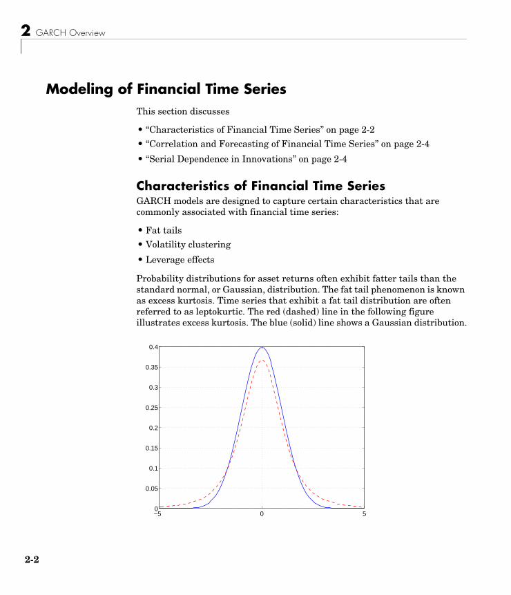
Probability distributions for asset returns often exhibit fatter tails than the standard normal, or Gaussian, distribution. The fat tail phenomenon is known as excess kurtosis. Time series that exhibit a fat tail distribution are often referred to as leptokurtic. The red (dashed) line in the following figure illustrates excess kurtosis. The blue (solid) line shows a Gaussian distribution.
−5 0 50
0.05
0.1
0.15
0.2
0.25
0.3
0.35
0.4

Modeling of Financial Time Series
2-3
In addition, financial time series usually exhibit a characteristic known as volatility clustering, in which large changes tend to follow large changes, and small changes tend to follow small changes. In either case, the changes from one period to the next are typically of unpredictable sign. Large disturbances, positive or negative, become part of the information set used to construct the variance forecast of the next period's disturbance. In this manner, large shocks of either sign are allowed to persist, and can influence the volatility forecasts for several periods.
Volatility clustering, or persistence, suggests a time-series model in which successive disturbances, although uncorrelated, are nonetheless serially dependent. The following figure illustrates this characteristic. It shows the daily returns of the New York Stock Exchange™ Composite Index (see “Data Sets” on page 1-11).
Volatility clustering (a type of heteroscedasticity) accounts for some but not all of the fat tail effect (or excess kurtosis) typically observed in financial data. A part of the fat tail effect can also result from the presence of non-Gaussian asset return distributions that just happen to have fat tails, such as Student’s t.
Finally, certain classes of asymmetric GARCH models are also capable of capturing the so-called leverage effect, in which asset returns are often
1 507 1014 1518 2025 2529 3027−0.08
−0.06
−0.04
−0.02
0
0.02
0.04
0.06
Ret
urn
NYSE Daily Returns

2 GARCH Overview
2-4
observed to be negatively correlated with changes is volatility. That is, for certain asset classes, most notably equities but excluding foreign exchange, volatility tends to rise in response to lower than expected returns and to fall in response to higher than expected returns. Such an effect suggests GARCH models that include an asymmetric response to positive and negative surprises.
Correlation and Forecasting of Financial Time SeriesIf you treat a financial time series as a sequence of random observations, this random sequence, or stochastic process, may exhibit some degree of correlation from one observation to the next. You can use this correlation structure to predict future values of the process based on the past history of observations. Exploiting the correlation structure, if any, allows you to decompose the time series into a deterministic component (i.e., the forecast), and a random component (i.e., the error, or uncertainty, associated with the forecast).
The following equation uses these components to represent a univariate model of an observed time series .
In this equation,
• represents the forecast, or deterministic component, of the current return as a function of any information known at time , including past innovations , past observations , and any other relevant explanatory time-series data, .
• is the random component. It represents the innovation in the mean of . Note that you can also interpret the random disturbance, or shock, , as the single-period-ahead forecast error.
Serial Dependence in InnovationsA common assumption when modeling financial time series is that the forecast errors (i.e., the innovations) are zero-mean random disturbances uncorrelated from one period to the next.
yt
yt f t 1– X,( ) εt+=
f t 1– X,( )t 1–
εt 1– εt 2– …, ,{ } yt 1– yt 2– …, ,{ }X
εt ytεt
E εt{ } 0=
E εtεT{ } 0= t T≠
Modeling of Financial Time Series
2-5
Although successive innovations are uncorrelated, they are not independent. In fact, an explicit generating mechanism for a GARCH innovations process,
, is
(2-1)
where is the conditional standard deviation derived from one of the conditional variance equations shown in “Conditional Variance Models” on page 2-6.
is a standardized, independent, identically distributed (i.i.d.) random draw from some specified probability distribution. The GARCH Toolbox provides two distributions for modeling GARCH processes: Gaussian and Student’s t. Eq. (2-1) illustrates that a GARCH innovations process simply rescales an i.i.d process such that the conditional standard deviation incorporates the serial dependence of the conditional variance equation. Equivalently, Eq. (2-1) also states that a standardized GARCH disturbance, , is itself an i.i.d. random variable .
Notice that GARCH models are consistent with various forms of efficient market theory, which state that asset returns observed in the past cannot improve the forecasts of asset returns in the future. Since GARCH innovations
are serially uncorrelated, GARCH modeling does not violate efficient market theory.
εt{ }
εt σtzt=
σt
zt
εt{ }zt{ }
εt σt⁄zt
εt{ }

2 GARCH Overview
2-6
Conditional Mean and Variance ModelsThis section describes the conditional mean and variance models that the GARCH Toolbox supports and offers some comments to help clarify their descriptions.
• “Conditional Mean Model” on page 2-6
• “Conditional Variance Models” on page 2-6
• “Comments on the Models” on page 2-9
Conditional Mean ModelThis general ARMAX(R,M,Nx) model for the conditional mean applies to all variance models.
(2-2)
with autoregressive coefficients , moving average coefficients , innovations , and returns . is an explanatory regression matrix in which each column is a time series and denotes the th row and th column.
The eigenvalues associated with the characteristic AR polynomial
must lie inside the unit circle to ensure stationarity. Similarly, the eigenvalues associated with the characteristic MA polynomial
must lie inside the unit circle to ensure invertibility.
Conditional Variance ModelsThe conditional variance of the innovations, , is by definition
(2-3)
yt C φiyt i–i 1=
R
∑ εt θjεt j–
j 1=
M
∑ βkX t k,( )k 1=
Nx
∑+ + + +=
φi{ } θj{ }εt{ } yt{ } X
X t k,( ) t k
λi{ }
λR φ1λR 1–
– φ2λR 2–
– …– φR–
λM θ1λM 1– θ2λ
M 2– … θM+ + + +
σt2
Vart 1– yt( ) Et 1– εt2
( ) σt2
= =
Conditional Mean and Variance Models
2-7
The key insight of GARCH lies in the distinction between conditional and unconditional variances of the innovations process . The term conditional implies explicit dependence on a past sequence of observations. The term unconditional is more concerned with long-term behavior of a time series and assumes no explicit knowledge of the past.
The various GARCH models characterize the conditional distribution of by imposing alternative parameterizations to capture serial dependence on the conditional variance of the innovations. “Comments on the Models” on page 2-9 further defines the conditional variance models.
GARCH(P,Q) Conditional VarianceThe general GARCH(P,Q) model for the conditional variance of innovations is
(2-4)
with constraints
Note that the basic GARCH(P,Q) model is a symmetric variance process, in that the sign of the disturbance is ignored.
GJR(P,Q) Conditional VarianceThe general GJR(P,Q) model for the conditional variance of the innovations with leverage terms is
(2-5)
εt{ }
εt
σt2 κ Giσt i–
2
i 1=
P
∑ Ajεt j–2
j 1=
Q
∑+ +=
Gii 1=
P
∑ Ajj 1=
Q
∑+ 1<
κ 0>
Gi 0≥ i 1 2 … P, , ,=
Aj 0≥ j 1 2 … Q, , ,=
σt2 κ Giσt 1–
2
i 1=
P
∑ Ajεt j–2
j 1=
Q
∑ LjSt j–– εt j–
2
j 1–
Q
∑+ + +=

2 GARCH Overview
2-8
where
and
EGARCH(P,Q) Conditional VarianceThe general EGARCH(P,Q) model for the conditional variance of the innovations with leverage terms and an explicit probability distribution assumption is
(2-6)
where
with degrees of freedom .
St j–– 1 εt j– 0<
0 otherwise
=
Gi
i 1=
P
∑ Aj
j 1=
Q
∑12--- Lj
j 1=
Q
∑+ + 1<
κ 0>
Gi 0≥ i 1 2 … P, , ,=
Aj 0≥ j 1 2 … Q, , ,=
Aj Lj+ 0≥ j 1 2 … Q, , ,=
log σt2 κ Gilogσt i–
2
i 1=
P
∑ Ajεt j–
σt j–
-------------- Eεt j–
σt j–
--------------
–
j 1=
Q
∑ Ljεt j–
σt j–
------------
j 1=
Q
∑+ + +=
E zt j–{ } Eεt j–
σt j–
--------------
2 π⁄ Gaussian
ν 2–π
------------
Γ ν 1–2
------------
Γ ν2---
----------------------⋅ Student’s t
= =
ν 2>

Conditional Mean and Variance Models
2-9
EGARCH(P,Q) models are treated as ARMA(P,Q) models for . Thus, the stationarity constraint for EGARCH(P,Q) models is included by ensuring that the eigenvalues of the characteristic polynomial
are inside the unit circle.
Note that EGARCH models are fundamentally different from GARCH and GJR models in that the standardized innovation, , serves as the forcing variable for both the conditional variance and the error. GARCH and GJR models allow for volatility clustering (i.e., persistence) by a combination of the and terms, whereas persistence in EGARCH models is entirely captured by the terms.
Comments on the ModelsThe econometrics literature is often vague and lacks consensus regarding the exact definition of any particular class of GARCH model. As a result, there are often discrepancies among software vendors, researchers, and references as to the exact functional form, or parameter constraints, or both, of almost all GARCH models. To help you reconcile some of these discrepancies, a few comments are useful:
• Although the functional form of a GARCH(P,Q) model (Eq. (2-4)) is quite standard, alternative positivity constraints exist. However, these alternatives involve additional nonlinear inequalities that are difficult to impose in practice, and do not affect the GARCH(1,1) model, which is by far the most common. In contrast, the standard linear positivity constraints imposed by the GARCH Toolbox are commonly used, and are straightforward to implement.
• Many references and software vendors refer to the GJR(P,Q) model (Eq. (2-5)) as a TGARCH, or Threshold GARCH, model. However, others make a very clear distinction between GJR(P,Q) and TGARCH(P,Q) models: a GJR(P,Q) model is a recursive equation for the conditional variance, whereas a TGARCH(P,Q) model is the identical recursive equation for the conditional standard deviation (see, for example, Hamilton [18] page 669, Bollerslev, et. al. [6] page 2970). Furthermore, additional discrepancies exist regarding whether or not to allow both negative and positive innovations to
logσt2
λP G1λP 1–
– G2λP 2–
– …– GP–
zt
Gi AjGi

2 GARCH Overview
2-10
affect the conditional variance process. The GJR(P,Q) model included in the GARCH Toolbox is relatively standard.
• The manner in which the GARCH Toolbox parameterizes GARCH(P,Q) and GJR(P,Q) models, Eq. (2-4) and Eq. (2-5), including constraints, allows you to interpret a GJR(P,Q) model as a straightforward extension of a GARCH(P,Q) model. Equivalently, you can interpret a GARCH(P,Q) model as a restricted GJR(P,Q) model with zero leverage terms. This latter interpretation is convenient for, among other things, estimation and hypothesis testing via likelihood ratios.
• For GARCH(P,Q) and GJR(P,Q) models, the lag lengths and , as well as the magnitudes of the coefficients and , determine the extent to which disturbances persist. These values then determine the minimum amount of presample data needed to initiate the simulation and estimation processes. Note that persistence in EGARCH models is entirely captured by the terms.
• Although the functional form of an EGARCH(P,Q) model (Eq. (2-6)) is relatively standard, it is not the same as Nelson's original (see Nelson [22]). Many forms of EGARCH(P,Q) models exist. Another popular form is
This EGARCH(P,Q) model form appears to offer an advantage in that it does not explicitly make any assumptions about the conditional probability distribution (i.e., whether the distribution of is Gaussian or Student’s t). However, this is not entirely true. Although no distribution is explicitly assumed in the above equation, generally such an assumption is required for forecasting as well as Monte Carlo simulation in the absence of user-specified presample data. In fact, the above equation can easily be rearranged to highlight the probability distribution.
The particular form of the EGARCH(P,Q) model, Eq. (2-6), implemented in the GARCH Toolbox is selected because it closely resembles Nelson's original form and is widely used.
• Although EGARCH(P,Q) models require no parameter constraints to ensure positive conditional variances, stationarity constraints are necessary. Since an EGARCH(P,Q) model is treated as an ARMA(P,Q) model for the
P QGi Aj
Gi
log σt2 κ Gilogσt i–
2
i 1=
P
∑ Ajεt j– Ljεt j–+
σt j–
--------------------------------------
j 1=
Q
∑+ +=
zt εt σt⁄( )=

Conditional Mean and Variance Models
2-11
logarithm of the conditional variance, the GARCH Toolbox imposes non-linear constraints on the coefficients to ensure that the eigenvalues of the characteristic polynomial are all inside the unit circle (see, for example, page 2969 of Bollerslev, Engle, and Nelson [6], and page 12 of Bollerslev, Chou, and Kroner [5]).
• The EGARCH(P,Q) and GJR(P,Q) models, Eq. (2-6) and Eq. (2-5), are both asymmetric models designed to capture the leverage effect, or negative correlation, between asset returns and volatility. Both the EGARCH(P,Q) and GJR(P,Q) models include leverage terms that explicitly take into account the sign as well as the magnitude of the innovation noise term. Although both models are designed to capture the leverage effect, the manner in which they do so is markedly different.
For EGARCH(P,Q) models, the leverage coefficients are applied to the actual innovations . For GJR(P,Q) models, the leverage coefficients enter the model through a Boolean indicator, or dummy, variable. For this reason, if the leverage effect does indeed hold, the leverage coefficients should be negative for EGARCH(P,Q) models and positive for GJR(P,Q) models. This is in contrast to GARCH(P,Q) models, in which the sign of the innovation is ignored.
• Although GARCH(P,Q) and GJR(P,Q) models, Eq. (2-4) and Eq. (2-5), include terms related to the model innovations, , EGARCH(P,Q) models, Eq. (2-6), include terms related to the standardized innovations,
, such that acts as the forcing variable for both the conditional variance and the error. In this respect, EGARCH(P,Q) models are fundamentally unique.
• Generally, there are no asymmetries in foreign exchange rates, and therefore asymmetric EGARCH(P,Q) and GJR(P,Q) conditional variance models are often inappropriate for modeling such return series.
Gi
Liεt i–
Li
εt ztσt=
zt εt σt⁄= zt

2 GARCH Overview
2-12
The Default ModelThe GARCH Toolbox default model is the simple (yet common) constant mean model with GARCH(1,1) Gaussian innovations, based on Eq. (2-2) and Eq. (2-4).
(2-7)
(2-8)
In the conditional mean model, Eq. (2-7), the returns, , consist of a simple constant, plus an uncorrelated, white noise disturbance, . This model is often sufficient to describe the conditional mean in a financial return series. Most financial return series do not require the comprehensiveness that an ARMAX model provides.
In the conditional variance model, Eq. (2-8), the variance forecast, , consists of a constant plus a weighted average of last period's forecast, , and last period's squared disturbance, . Although financial return series, as defined in Eq. (1-1) and Eq. (1-2), typically exhibit little correlation, the squared returns often indicate significant correlation and persistence. This implies correlation in the variance process, and is an indication that the data is a candidate for GARCH modeling.
Although simplistic, the default model shown in Eq. (2-7) and Eq. (2-8) has several benefits:
• It represents a parsimonious model that requires you to estimate only four parameters ( , , , and ). According to Box and Jenkins [8], the fewer parameters to estimate, the less that can go wrong. Elaborate models often fail to offer real benefits when forecasting (see Hamilton [18], page 109).
• The simple GARCH(1,1) model captures most of the variability in most return series. Small lags for and are common in empirical applications. Typically, GARCH(1,1), GARCH(2,1), or GARCH(1,2) models are adequate for modeling volatilities even over long sample periods (see Bollerslev, Chou, and Kroner [5], pages 10 and 22).
yt C εt+=
σt2 κ G1σt 1–
2A1εt 1–
2+ +=
ytεt
σt2
σt 1–2
εt 1–2
C κ G1 A1
P Q

Primary Toolbox Functions
2-13
Primary Toolbox FunctionsUse of the GARCH Toolbox focuses on three high-level processing functions: garchfit, garchpred, and garchsim, for model estimation, forecasting, and Monte Carlo simulation, respectively. A fourth function, garchinfer, infers the innovations and conditional standard deviations via inverse filtering, and is closely related to garchfit in that they both call the appropriate objective function.
These functions use a GARCH specification structure to share information about the specified model. The specification structure contains the model orders for the chosen conditional mean and variance models, and the parameters for those models. All these functions accept a specification structure as input, but only garchfit can update the structure and provide it as an output. (See “GARCH Specification Structure” on page 3-1 for detailed information about the structure.)
An analysis process using real-world data might involve calling these processing functions:
garchfit Estimates the model parameters. garchfit can accept a specification structure as an input. If you provide only the model orders for the chosen conditional mean and variance model, garchfit populates it with the coefficients resulting from the estimation process. If you provide, in addition, valid coefficients, garchfit uses them as initial estimates that are refined by the estimation process. If you provide no specification structure, garchfit assumes the default model (see “The Default Model” on page 2-12).
In all cases, garchfit returns an updated specification structure, which encapsulates parameter estimates. This output structure is of the same form as the input structure, and you can use it as an input for further modeling.

2 GARCH Overview
2-14
garchpred Forecasts returns and conditional standard deviations. It accepts as input the specification structure provided by the estimation engine garchfit. You can also use garchpred to forecast volatility of asset returns over multiperiod holding intervals, or to forecast the standard errors of conditional mean forecasts.
garchsim Simulates one or more sample paths for the return series, innovations, and conditional standard deviation processes, for the specified conditional mean and variance model. You can use these sample paths to perform Monte Carlo simulation of a given process.
Analysis and Estimation Example Using the Default Model
2-15
Analysis and Estimation Example Using the Default ModelThe example in this section uses the GARCH Toolbox default model to model a foreign exchange series. Specifically, the example explores
• “Preestimation Analysis” on page 2-15
• “Parameter Estimation” on page 2-23
• “Postestimation Analysis” on page 2-26
Note Due to platform differences, the estimation results you obtain when you recreate this example may differ slightly from those shown in the text. These differences will propagate through any subsequent examples that use the estimation results as input. These differences, however, do not affect the outcome of the examples.
For more information see “Model Selection and Analysis” on page 8-1.
Preestimation AnalysisWhen estimating the parameters of a composite conditional mean/variance model, you may occasionally encounter convergence problems. For example, the estimation may appear to stall, showing little or no progress. It may terminate prematurely prior to convergence. Or, it may converge to an unexpected, suboptimal solution.
You can avoid many of these difficulties by performing a prefit analysis. This section uses an example to show techniques such as plotting the return series, and examining the ACF and PACF, as well as some preliminary tests, including Engle’s ARCH test and the Q-test. The goal is to avoid convergence problems by selecting the simplest model that adequately describes your data.
The preestimation analysis loads the data in the form of a price series, then converts the price series to a return series. It checks the return series for correlation, and quantifies the correlation.
1 Load the raw data: daily exchange rate. Start by loading the MATLAB binary file garchdata.mat, and examining its contents using the Workspace Browser.

2 GARCH Overview
2-16
load garchdata
The data consists of three single-column vectors of different lengths, DEM2GBP, NASDAQ, and NYSE. Each vector is a separate price series for the named group. (See “Data Sets” on page 1-11 for more information about these data sets.) You can also use the whos command to see all the variables in the current workspace.
whos
Name Size Bytes Class
DEM2GBP 1975x1 15800 double array NASDAQ 3028x1 24224 double array NYSE 3028x1 24224 double array
Grand total is 8031 elements using 64248 bytes
This example uses DEM2GBP, which contains daily price observations of the Deutschemark/British Pound foreign exchange rate. Use the MATLAB plot function to examine the data.
plot([0:1974],DEM2GBP)set(gca,'XTick',[1 659 1318 1975])set(gca,'XTickLabel',{'Jan 1984' 'Jan 1986' 'Jan 1988' ... 'Jan 1992'})

Analysis and Estimation Example Using the Default Model
2-17
ylabel('Exchange Rate')title('Deutschmark/British Pound Foreign Exchange Rate')
Note The set command allows you to set object properties. This example uses it to set the position of and relabel the x-axis ticks of the current figure.
2 Convert the prices to a return series. Because GARCH modeling assumes a return series, you need to convert the prices to returns. Use the utility function price2ret, and then examine the result.
dem2gbp = price2ret(DEM2GBP);
The workspace information shows both the 1975-point price series and the 1974-point return series derived from it.
Now, use the MATLAB plot function to see the return series. Notice the presence of volatility clustering in the raw return series.
plot(dem2gbp)set(gca,'XTick',[1 659 1318 1975])
Jan 1984 Jan 1986 Jan 1988 Jan 19922.6
2.8
3
3.2
3.4
3.6
3.8
4
4.2
Exc
hang
e R
ate
Deutschmark/British Pound Foreign Exchange Rate

2 GARCH Overview
2-18
set(gca,'XTickLabel',{'Jan 1984' 'Jan 1986' 'Jan 1988' ... 'Jan 1992'})ylabel('Return')title('Deutschmark/British Pound Daily Returns')
3 Check for correlation in the return series. You can check qualitatively for correlation in the raw return series by calling the functions autocorr and parcorr to examine the sample autocorrelation function (ACF) and partial-autocorrelation (PACF) function, respectively.
The autocorr function computes and displays the sample ACF of the returns, along with the upper and lower standard deviation confidence bounds, based on the assumption that all autocorrelations are zero beyond lag zero.
autocorr(dem2gbp)title('ACF with Bounds for Raw Return Series')
Jan 1984 Jan 1986 Jan 1988 Jan 1992−0.03
−0.02
−0.01
0
0.01
0.02
0.03
0.04R
etur
nDeutschmark/British Pound Daily Returns

Analysis and Estimation Example Using the Default Model
2-19
Similarly, the parcorr function displays the sample PACF with upper and lower confidence bounds.
parcorr(dem2gbp)title('PACF with Bounds for Raw Return Series')
0 5 10 15 20−0.2
0
0.2
0.4
0.6
0.8
Lag
Sam
ple
Aut
ocor
rela
tion
ACF with Bounds for Raw Return Series

2 GARCH Overview
2-20
Since the individual ACF values can have large variances and can also be autocorrelated, you should view the sample ACF and PACF with care (see Box, Jenkins, Reinsel [8], pages 34 and 186). However, as preliminary identification tools, the ACF and PACF provide some indication of the broad correlation characteristics of the returns. From these figures for the ACF and PACF, there is very little indication that you need to use any correlation structure in the conditional mean. Also, notice the similarity between the graphs.
4 Check for correlation in the squared returns. Although the ACF of the observed returns exhibits little correlation, the ACF of the squared returns may still indicate significant correlation and persistence in the second-order moments. Check this by plotting the ACF of the squared returns.
autocorr(dem2gbp.^2)title('ACF of the Squared Returns')
0 5 10 15 20−0.2
0
0.2
0.4
0.6
0.8
Lag
Sam
ple
Par
tial A
utoc
orre
latio
ns
PACF with Bounds for Raw Return Series

Analysis and Estimation Example Using the Default Model
2-21
This figure shows that, although the returns themselves are largely uncorrelated, the variance process exhibits some correlation. This is consistent with the earlier discussion in the section, “The Default Model” on page 2-12. Note that the ACF shown in this figure appears to die out slowly, indicating the possibility of a variance process close to being nonstationary.
Note The syntax in the preceding command, an operator preceded by the dot operator (.), indicates that the operation is performed on an element-by-element basis. In the preceding command, dem2gbp.^2 indicates that each element of the vector dem2gbp is squared.
5 Quantify the correlation. You can quantify the preceding qualitative checks for correlation using formal hypothesis tests, such as the Ljung-Box-Pierce Q-test and Engle's ARCH test.
The function lbqtest implements the Ljung-Box-Pierce Q-test for a departure from randomness based on the ACF of the data. The Q-test is most often used as a postestimation lack-of-fit test applied to the fitted
0 5 10 15 20−0.2
0
0.2
0.4
0.6
0.8
Lag
Sam
ple
Aut
ocor
rela
tion
ACF of the Squared Returns

2 GARCH Overview
2-22
innovations (i.e., residuals). In this case, however, you can also use it as part of the prefit analysis because the default model assumes that returns are just a simple constant plus a pure innovations process. Under the null hypothesis of no serial correlation, the Q-test statistic is asymptotically Chi-Square distributed (see Box, Jenkins, Reinsel [8], page 314).
The function archtest implements Engle's test for the presence of ARCH effects. Under the null hypothesis that a time series is a random sequence of Gaussian disturbances (i.e., no ARCH effects exist), this test statistic is also asymptotically Chi-Square distributed (see Engle [12], pages 999-1000).
Both functions return identical outputs. The first output, H, is a Boolean decision flag. H = 0 implies that no significant correlation exists (i.e., do not reject the null hypothesis). H = 1 means that significant correlation exists (i.e., reject the null hypothesis). The remaining outputs are the P-value (pValue), the test statistic (Stat), and the critical value of the Chi-Square distribution (CriticalValue).
Ljung-Box-Pierce Q-Test. Using lbqtest, you can verify, at least approximately, that no significant correlation is present in the raw returns when tested for up to 10, 15, and 20 lags of the ACF at the 0.05 level of significance.
[H,pValue,Stat,CriticalValue] = ... lbqtest(dem2gbp-mean(dem2gbp),[10 15 20]',0.05);[H pValue Stat CriticalValue]
ans = 0 0.7278 6.9747 18.3070 0 0.2109 19.0628 24.9958 0 0.1131 27.8445 31.4104
However, there is significant serial correlation in the squared returns when you test them with the same inputs.
[H,pValue,Stat,CriticalValue] = ... lbqtest((dem2gbp-mean(dem2gbp)).^2,[10 15 20]',0.05);[H pValue Stat CriticalValue]

Analysis and Estimation Example Using the Default Model
2-23
ans = 1.0000 0 392.9790 18.3070 1.0000 0 452.8923 24.9958 1.0000 0 507.5858 31.4104
Engle's ARCH Test. You can also perform Engle’s ARCH test using the function archtest. This test also shows significant evidence in support of GARCH effects (i.e., heteroscedasticity).
[H,pValue,Stat,CriticalValue] = ... archtest(dem2gbp-mean(dem2gbp),[10 15 20]',0.05);[H pValue Stat CriticalValue]
ans = 1.0000 0 192.3783 18.3070 1.0000 0 201.4652 24.9958 1.0000 0 203.3018 31.4104
Each of these examples extracts the sample mean from the actual returns. This is consistent with the definition of the conditional mean equation of the default model, in which the innovations process is , and is the mean of .
Parameter EstimationThis section continues the example begun in “Preestimation Analysis” on page 2-15. It estimates model parameters, then examines the estimated GARCH model.
1 Estimate the Model Parameters. The presence of heteroscedasticity, shown in the previous analysis, indicates that GARCH modeling is appropriate. Use the estimation function garchfit to estimate the model parameters. Assume the default GARCH model described in the section “The Default Model” on page 2-12. This only requires that you specify the return series of interest as an argument to the function garchfit.
εt yt C–= Cyt
2 GARCH Overview
2-24
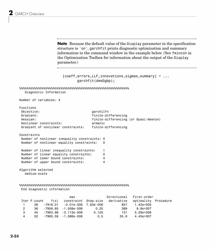
Note Because the default value of the Display parameter in the specification structure is 'on', garchfit prints diagnostic optimization and summary information to the command window in the example below. (See fmincon in the Optimization Toolbox for information about the output of the Display parameter.)
[coeff,errors,LLF,innovations,sigmas,summary] = ... garchfit(dem2gbp);
%%%%%%%%%%%%%%%%%%%%%%%%%%%%%%%%%%%%%%%%%%%%%%%%%%%%%%%%%%% Diagnostic Information
Number of variables: 4
Functions Objective: garchllfn Gradient: finite-differencing Hessian: finite-differencing (or Quasi-Newton) Nonlinear constraints: armanlc Gradient of nonlinear constraints: finite-differencing
Constraints Number of nonlinear inequality constraints: 0 Number of nonlinear equality constraints: 0 Number of linear inequality constraints: 1 Number of linear equality constraints: 0 Number of lower bound constraints: 4 Number of upper bound constraints: 4
Algorithm selected medium-scale
%%%%%%%%%%%%%%%%%%%%%%%%%%%%%%%%%%%%%%%%%%%%%%%%%%%%%%%%%%% End diagnostic information
max Directional First-order Iter F-count f(x) constraint Step-size derivative optimality Procedure 1 28 -7916.01 -2.01e-006 7.63e-006 857 1.42e+005 2 36 -7959.65 -1.508e-006 0.25 389 9.8e+007 3 45 -7963.98 -3.113e-006 0.125 131 5.29e+006 4 52 -7965.59 -1.586e-006 0.5 55.9 4.45e+007

Analysis and Estimation Example Using the Default Model
2-25
5 65 -7966.9 -1.574e-006 0.00781 101 1.46e+007 6 74 -7969.46 -2.201e-006 0.125 14.9 2.77e+007 7 83 -7973.56 -2.663e-006 0.125 36.6 1.45e+007 8 90 -7982.09 -1.332e-006 0.5 -6.39 5.59e+006 9 103 -7982.13 -1.399e-006 0.00781 6.49 1.32e+006 10 111 -7982.53 -1.049e-006 0.25 12.5 1.87e+007 11 120 -7982.56 -1.186e-006 0.125 3.72 3.8e+006 12 128 -7983.69 -1.11e-006 0.25 0.184 4.91e+006 13 134 -7983.91 -7.813e-007 1 0.732 1.22e+006 14 140 -7983.98 -9.265e-007 1 0.186 1.17e+006 15 146 -7984 -8.723e-007 1 0.0427 9.52e+005 16 154 -7984 -8.775e-007 0.25 0.0152 6.33e+005 17 160 -7984 -8.75e-007 1 0.00197 6.98e+005 18 166 -7984 -8.763e-007 1 0.000931 7.38e+005 19 173 -7984 -8.759e-007 0.5 0.000469 7.37e+005 20 179 -7984 -8.761e-007 1 0.00012 7.22e+005 21 199 -7984 -8.761e-007 -6.1e-005 0.0167 7.37e+005 Hessian modified twice 22 213 -7984 -8.761e-007 0.00391 0.00582 7.26e+005 Hessian modified twice Optimization terminated successfully: Search direction less than 2*options.TolX and maximum constraint violation is less than options.TolCon No Active Constraints
2 Examine the Estimated GARCH Model. Now that the estimation is complete, you can display the parameter estimates and their standard errors using the function garchdisp,
garchdisp(coeff,errors)
Mean: ARMAX(0,0,0); Variance: GARCH(1,1)
Conditional Probability Distribution: Gaussian Number of Parameters Estimated: 4
Standard T Parameter Value Error Statistic ----------- ----------- ------------ ----------- C -6.1919e-005 8.4331e-005 -0.7342 K 1.0761e-006 1.323e-007 8.1341 GARCH(1) 0.80598 0.016561 48.6685 ARCH(1) 0.15313 0.013974 10.9586
If you substitute these estimates in the definition of the default model, Eq. (2-7) and Eq. (2-8), the estimation process implies that the constant

2 GARCH Overview
2-26
conditional mean/GARCH(1,1) conditional variance model that best fits the observed data is
where = GARCH(1) = 0.80598 and = ARCH(1) = 0.15313. In addition, = C = -6.1919e-005 and = K = 1.0761e-006.
Postestimation AnalysisThe postestimation analysis continues the example begun in “Preestimation Analysis” on page 2-15 and continued in “Parameter Estimation” on page 2-23. This part of the example starts by comparing the residuals, conditional standard deviations, and returns. It then uses plots and quantitative techniques to compare correlation of the standardized innovations.
1 Compare the Residuals, Conditional Standard Deviations, and Returns. In addition to the parameter estimates and standard errors, garchfit also returns the optimized log-likelihood function value (LLF), the residuals (innovations), and conditional standard deviations (sigmas). Use the function garchplot to inspect the relationship between the innovations (i.e., residuals) derived from the fitted model, the corresponding conditional standard deviations, and the observed returns.
garchplot(innovations,sigmas,dem2gbp)
yt 6.1919e-005– εt+=
σt2
1.0761e-006 0.80598σt 1–2
0.15313εt 1–2
+ +=
G1 A1C κ

Analysis and Estimation Example Using the Default Model
2-27
Notice that both the innovations (top plot) and the returns (bottom plot) exhibit volatility clustering. Also, notice that the sum,
= 0.80598 + 0.15313, is 0.95911, which is close to the integrated, nonstationary boundary given by the constraints associated with Eq. (2-4).
2 Plot and Compare the Correlation of the Standardized Innovations. Although the figure in step 1 shows that the fitted innovations exhibit volatility clustering, if you plot the standardized innovations (the innovations divided by their conditional standard deviation), they appear generally stable with little clustering.
plot(innovations./sigmas)ylabel('Innovation')title('Standardized Innovations')
0 500 1000 1500 2000−0.05
0
0.05Innovations
Inno
vatio
n
0 500 1000 1500 20000
0.005
0.01
0.015Conditional Standard Deviations
Sta
ndar
d D
evia
tion
0 500 1000 1500 2000−0.05
0
0.05Returns
Ret
urn
G1 A1+

2 GARCH Overview
2-28
If you plot the ACF of the squared standardized innovations, they also show no correlation.
autocorr((innovations./sigmas).^2)title('ACF of the Squared Standardized Innovations')
0 500 1000 1500 2000−8
−6
−4
−2
0
2
4
6
Inno
vatio
n
Standardized Innovations

Analysis and Estimation Example Using the Default Model
2-29
Now compare the ACF of the squared standardized innovations in this figure to the ACF of the squared returns prior to fitting the default model (See “Preestimation Analysis” on page 2-15, step 4). The comparison shows that the default model sufficiently explains the heteroscedasticity in the raw returns.
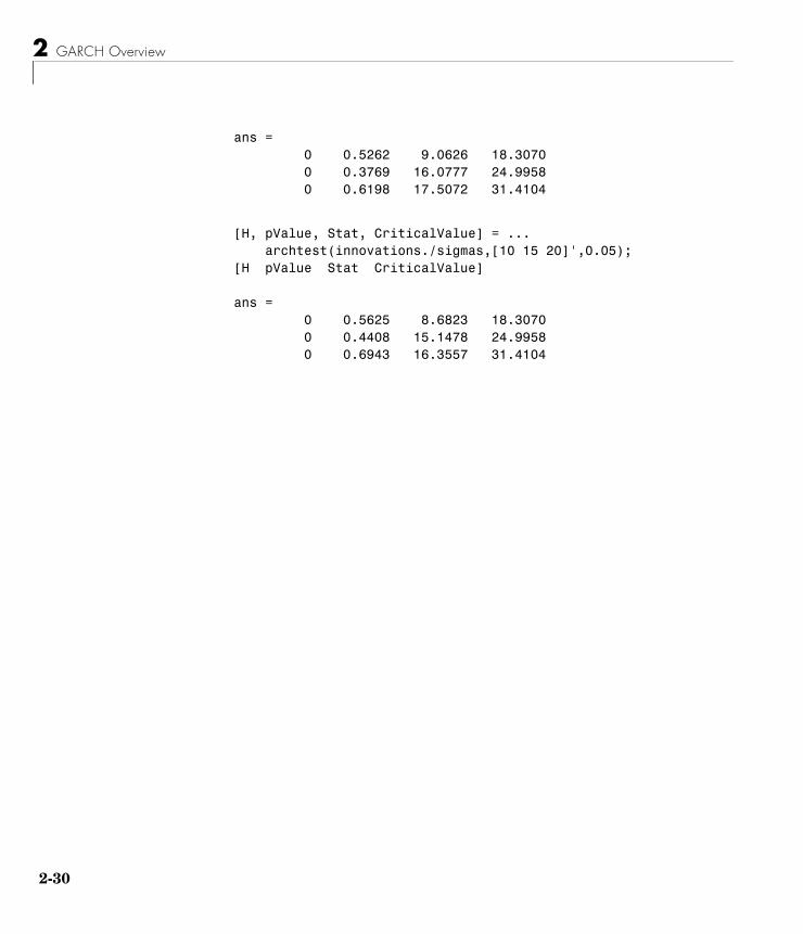
3 Quantify and Compare Correlation of the Standardized Innovations. Compare the results below of the Q-test and the ARCH test with the results of these same tests in the preestimation analysis. In the preestimation analysis, both the Q-test and the ARCH test indicate rejection (H = 1 with pValue = 0) of their respective null hypotheses, showing significant evidence in support of GARCH effects. In the postestimate analysis, using standardized innovations based on the estimated model, these same tests indicate acceptance (H = 0 with highly significant pValues) of their respective null hypotheses and confirm the explanatory power of the default model.
[H, pValue,Stat,CriticalValue] = ... lbqtest((innovations./sigmas).^2,[10 15 20]',0.05);[H pValue Stat CriticalValue]
0 5 10 15 20−0.2
0
0.2
0.4
0.6
0.8
Lag
Sam
ple
Aut
ocor
rela
tion
ACF of the Squared Standardized Innovations
2 GARCH Overview
2-30
ans = 0 0.5262 9.0626 18.3070 0 0.3769 16.0777 24.9958 0 0.6198 17.5072 31.4104
[H, pValue, Stat, CriticalValue] = ... archtest(innovations./sigmas,[10 15 20]',0.05);[H pValue Stat CriticalValue]
ans = 0 0.5625 8.6823 18.3070 0 0.4408 15.1478 24.9958 0 0.6943 16.3557 31.4104

3GARCH Specification Structure
“GARCH Specification Structure” includes these sections:
Introduction (p. 3-2) Introduces the GARCH specification structure and explains how the primary analysis and modeling functions operate on the structure.
Equation Variables and Parameter Names (p. 3-4)
Associates the variables used in the model equations (“Conditional Mean and Variance Models” on page 2-6) with their corresponding parameters in the specification structure.
Examples of Specification Structures (p. 3-5)
Uses examples of specification structures to interpret their contents.
Reading and Writing Specification Structures (p. 3-8)
Describes the creation and modification of a specification structure, as well as the retrieval of values from it.

3 GARCH Specification Structure
3-2
IntroductionThe GARCH Toolbox maintains the parameters that define a model and control the estimation process in a specification structure.
For the default model (see “The Default Model” on page 2-12), garchfit can create the specification structure and store the model orders and estimated parameters in it. For more complex models, you must use the function garchset to explicitly specify, in a specification structure, the conditional variance model you want, the mean and variance model orders, and possibly the initial coefficient estimates.
The primary analysis and modeling functions, garchfit, garchpred, and garchsim, all operate on the specification structure. This table describes how each function uses the specification structure.
Function Description Use of GARCH Specification Structure
garchfit Estimates the parameters of a conditional mean specification of ARMAX form and a conditional variance specification of GARCH, GJR, or EGARCH form.
Input. Optionally accepts a GARCH specification structure as input. If the structure contains the model orders (R, M, P, Q) but no coefficient vectors (C, AR, MA, Regress, K, ARCH, GARCH, Leverage), garchfit uses maximum likelihood to estimate the coefficients for the specified mean and variance models. If the structure contains coefficient vectors, garchfit uses them as initial estimates for further refinement. If you provide no specification structure, garchfit assumes, and returns, a specification structure for the default model (see “The Default Model” on page 2-12).
Output. Returns a specification structure that contains a fully specified ARMAX/GARCH model.

Introduction
3-3
Note See the garchset function reference page for descriptions of all the specification structure parameters.
garchpred Provides minimum-mean-square-error (MMSE) forecasts of the conditional mean and standard deviation of a return series, for a specified number of periods into the future.
Input. Requires a GARCH specification structure that contains the coefficient vectors for the model for which garchpred is to forecast the conditional mean and standard deviation.
Output. garchpred does not modify or return the specification structure.
garchsim Uses Monte Carlo methods to simulates sample paths for return series, innovations, and conditional standard deviation processes.
Input. Requires a GARCH specification structure that contains the coefficient vectors for the model for which garchsim is to simulate sample paths.
Output. garchsim does not modify or return the specification structure.
Function Description Use of GARCH Specification Structure
3 GARCH Specification Structure
3-4
Equation Variables and Parameter NamesFor the most part, the names of specification structure parameters that define the ARMAX and GARCH models reflect the variable names of their corresponding components in the conditional mean and variance model equations (see “Conditional Mean and Variance Models” on page 2-6).
Conditional Mean ModelIn the conditional mean model,
• R and M represent the order of the ARMA(R,M) conditional mean model.
• C represents the constant .
• AR represents the R-element autoregressive coefficient vector .
• MA represents the M-element moving average coefficient vector .
• Regress represents the regression coefficients .
Unlike the other components of the conditional mean equation, has no representation in the GARCH specification structure. is an optional matrix of returns that some toolbox functions use as explanatory variables in the regression component of the conditional mean. For example, could contain return series of a suitable market index collected over the same period as the return series . Toolbox functions that allow the use of a regression matrix provide a separate argument by which you can specify it.
Conditional Variance ModelsIn the conditional variance models
• P and Q represent the order of the GARCH(P,Q), GJR(P,Q), or EGARCH(P,Q) conditional variance model.
• K represents the constant .
• GARCH represents the P-element coefficient vector .
• ARCH represents the Q-element coefficient vector .
• Leverage represents the Q-element leverage coefficient vector, , for asymmetric EGARCH(P,Q) and GJR(P,Q) models.
C
φi
θj
βk
XX
X
y
κGi
Aj
Lj

Examples of Specification Structures
3-5
Examples of Specification StructuresThe following example shows the fields of the specification structure, coeff, for the estimated default model from “Analysis and Estimation Example Using the Default Model” on page 2-15. The term to the left of the colon (:) is the parameter name.
coeff
coeff = Comment: 'Mean: ARMAX(0,0,0); Variance: GARCH(1,1)' Distribution: 'Gaussian' C: -6.1919e-005 VarianceModel: 'GARCH' P: 1 Q: 1 K: 1.0761e-006 GARCH: 0.8060 ARCH: 0.1531
When you display a specification structure, only the fields that are applicable to the specified model are displayed. Notice that R = M = 0 for this model, and so are not displayed.
By default, the Comment field shown above is automatically generated by garchset and garchfit. It summarizes the ARMAX and GARCH models used for the conditional mean and variance equations. You can use garchset to set the value of the Comment field, but the value you give it will replace this summary statement.
Following is the display for the MA(1)/GJR(1,1) estimated model from the example “Specifying Presample Data” on page 5-19. Notice that length(MA) = M, length(GARCH) = P, and length(ARCH) = Q.
coeff = Comment: 'Mean: ARMAX(0,1,0); Variance: GJR(1,1)' Distribution: 'Gaussian' M: 1 C: 5.6403e-004 MA: 0.2501 VarianceModel: 'GJR' P: 1

3 GARCH Specification Structure
3-6
Q: 1 K: 1.1907e-005 GARCH: 0.6945 ARCH: 0.0249 Leverage: 0.2454 Display: 'off'
If you had created the specification structure for the same MA(1)/GJR(1,1) example, but had not yet estimated the model coefficients, this is what you would see if you displayed the specification structure.
spec = garchset('VarianceModel','GJR','M',1,'P',1,'Q',1,... 'Display','off')
spec = Comment: 'Mean: ARMAX(0,1,?); Variance: GJR(1,1)' Distribution: 'Gaussian' M: 1 C: [] MA: [] VarianceModel: 'GJR' P: 1 Q: 1 K: [] GARCH: [] ARCH: [] Leverage: [] Display: 'off'
The empty matrix symbols, [], indicate that these fields are required for the specified model, but have not yet been assigned values. For the specification to be complete, these fields must be assigned valid values. You can use garchset to assign values, e.g., as initial parameter estimates, to these fields. You can also pass such a specification structure to garchfit, which uses the parameters it estimates to complete the model specification. You cannot pass such a structure to garchsim, garchinfer, or garchpred. These functions require complete specifications.

Examples of Specification Structures
3-7
Note See the garchset function reference page for descriptions of all the specification structure fields.

3 GARCH Specification Structure
3-8
Reading and Writing Specification StructuresThis section discusses
• “Creating and Modifying a Specification Structure” on page 3-8
• “Retrieving Specification Structure Values” on page 3-11
Creating and Modifying a Specification StructureIn general, you must use the function garchset to initially create a specification structure that, at a minimum, contains the chosen variance model and the mean and variance model orders. The only exception is the default model, for which garchfit can create a specification structure. The model parameters you provide must specify a valid model.
When you create a specification structure, you can specify both the conditional mean and variance models. Alternatively, you can specify either the conditional mean or the conditional variance model. If you do not specify both models, garchset assigns default parameters to the one you did not specify. For the conditional mean, the default is a constant ARMA(0,0,?) model. For the conditional variance, the default is a constant GARCH(0,0) model. The question mark (?) indicates that garchset doesn’t know if you intend to include a regression component (see “Regression Components in Conditional Mean Models” on page 7-1).
The following examples create specification structures and display the results. Note that you only need to type the leading characters that uniquely identify the parameter. As illustrated here, garchset ignores case for parameter names.
The Default ModelThis is a sampling of statements that all create specification structures for the default model.
spec = garchset('R',0,'m',0,'P',1,'Q',1);
spec = garchset('p',1,'Q',1);
spec = garchset;

Reading and Writing Specification Structures
3-9
The output of each command is the same. The Comment field summarizes the model. Because R = M = 0, the fields R, M, AR, and MA are not displayed.
spec = Comment: 'Mean: ARMAX(0,0,?); Variance: GARCH(1,1)' Distribution: 'Gaussian' C: [] VarianceModel: 'GARCH' P: 1 Q: 1 K: [] GARCH: [] ARCH: []
ARMA(0,0)/GJR(1,1)This command accepts the constant default for the mean model.
spec = garchset('VarianceModel','GJR','P',1,'Q',1)
spec = Comment: 'Mean: ARMAX(0,0,?); Variance: GJR(1,1)' Distribution: 'Gaussian' C: [] VarianceModel: 'GJR' P: 1 Q: 1 K: [] GARCH: [] ARCH: [] Leverage: []
AR(2)/GARCH(1,2) with Initial Parameter EstimatesFor this command, garchset infers the model orders from the lengths of the coefficient vectors. garchset assumes a GARCH(P,Q) conditional variance process as the default.
spec = garchset('C',0,'AR',[0.5 -0.8],'K',0.0002,... 'GARCH',0.8,'ARCH',[0.1 0.05])
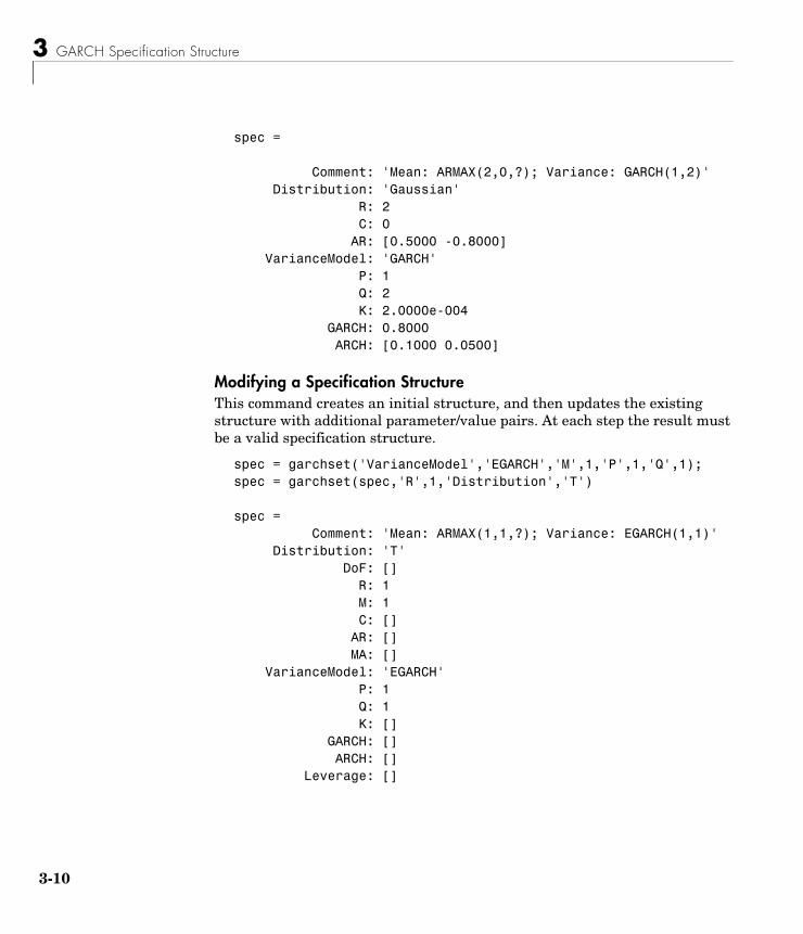
3 GARCH Specification Structure
3-10
spec =
Comment: 'Mean: ARMAX(2,0,?); Variance: GARCH(1,2)' Distribution: 'Gaussian' R: 2 C: 0 AR: [0.5000 -0.8000] VarianceModel: 'GARCH' P: 1 Q: 2 K: 2.0000e-004 GARCH: 0.8000 ARCH: [0.1000 0.0500]
Modifying a Specification StructureThis command creates an initial structure, and then updates the existing structure with additional parameter/value pairs. At each step the result must be a valid specification structure.
spec = garchset('VarianceModel','EGARCH','M',1,'P',1,'Q',1);spec = garchset(spec,'R',1,'Distribution','T')
spec = Comment: 'Mean: ARMAX(1,1,?); Variance: EGARCH(1,1)' Distribution: 'T' DoF: [] R: 1 M: 1 C: [] AR: [] MA: [] VarianceModel: 'EGARCH' P: 1 Q: 1 K: [] GARCH: [] ARCH: [] Leverage: []

Reading and Writing Specification Structures
3-11
Retrieving Specification Structure ValuesThe function garchget retrieves the values of the specification structure fields.
This example creates a specification structure, spec, by providing the model coefficients, and allowing garchset to infer the model orders from the lengths of these vectors. garchset assumes the GARCH(P,Q) default variance model. The example then uses garchget to retrieve the variance model and the model orders for the conditional mean. Note that you only need to type the leading characters that uniquely identify the parameter. As illustrated here, garchget ignores case for parameter names.
spec = garchset('C',0,'AR',[0.5 -0.8],'K',0.0002,... 'GARCH',0.8,'ARCH',[0.1 0.05])spec =
Comment: 'Mean: ARMAX(2,0,?); Variance: GARCH(1,2)' Distribution: 'Gaussian' R: 2 C: 0 AR: [0.5000 -0.8000] VarianceModel: 'GARCH' P: 1 Q: 2 K: 2.0000e-004 GARCH: 0.8000 ARCH: [0.1000 0.0500]
R = garchget(spec,'R')
R = 2
M = garchget(spec,'m')
M = 0
var = garchget(spec,'VarianceModel')
var = GARCH

3 GARCH Specification Structure
3-12
4
Simulation
“Simulation” includes these sections:
Simulating Sample Paths (p. 4-2) Shows you how to simulate single and multiple paths for return series, innovations, and conditional standard deviation processes.
Presample Data (p. 4-6) Explains the use of automatically generated and user-supplied presample data. For automatically generated presample data, this section also discusses response tolerance and the minimization of transient effects.

4 Simulation
4-2
Simulating Sample Paths• “Introduction” on page 4-2
• “Simulating a Single Path” on page 4-3
• “Simulating Multiple Paths” on page 4-4
IntroductionGiven models for the conditional mean and variance (see “Conditional Mean and Variance Models” on page 2-6), the function garchsim can simulate one or more sample paths for return series, innovations, and conditional standard deviation processes.
The section “Analysis and Estimation Example Using the Default Model” on page 2-15 uses the default GARCH(1,1) model to model the Deutschmark/British pound foreign exchange series. These examples use the resulting model
to simulate sample paths for return series, innovations, and conditional standard deviation processes.
Use the following commands to restore your workspace if necessary. The text of this example omits the display output of the estimation to save space.
load garchdatadem2gbp = price2ret(DEM2GBP);[coeff,errors,LLF,innovations,sigmas] = garchfit(dem2gbp);coeff
coeff = Comment: 'Mean: ARMAX(0,0,0); Variance: GARCH(1,1)' Distribution: 'Gaussian' C: -6.1919e-005 VarianceModel: 'GARCH' P: 1 Q: 1 K: 1.0761e-006
yt 6.1919e-005– εt+=
σt2
1.0761e-006 0.80598σt 1–2
0.15313εt 1–2
+ +=

Simulating Sample Paths
4-3
GARCH: 0.8060 ARCH: 0.1531
Simulating a Single PathThis code generates a single path of 1000 observations. Assuming there are 250 trading days per year, this is roughly fours years’ worth of daily data. (“Introduction” on page 4-2 tells you how to generate coeff for use in this example.)
[e,s,y] = garchsim(coeff,1000);
The Workspace Browser shows the result to be a single realization of 1000 observations each for the innovations , conditional standard deviations
, and returns processes. These processes are designated by the output variables e, s, and y, respectively.
Now plot the garchsim output data to see what it looks like.
garchplot(e,s,y)
εt{ }σt{ } yt{ }

4 Simulation
4-4
Note If you do not specify the number of observations, the default is 100. For example, [e,s,y] = garchsim(coeff) produces a single path of 100 observations.
Simulating Multiple PathsIn some cases, you may need multiple realizations. This example uses the same model to simulate 1000 paths of 200 observations each. (“Introduction” on page 4-2 tells you how to generate coeff for use in this example.)
[e,s,y] = garchsim(coeff,200,1000);
In this example, the , , and processes are 200-by-1000 element matrices. These are relatively large arrays, and demand large chunks of memory. In fact, because of the way the GARCH Toolbox manages transients, simulating this data requires more memory than the 4800000 bytes indicated in the Workspace Browser. (See “Automatically Generated Presample Data” on page 4-6 for more information about transients.)
0 200 400 600 800 1000−0.05
0
0.05Innovations
Inno
vatio
n
0 200 400 600 800 10000
0.01
0.02Conditional Standard Deviations
Sta
ndar
d D
evia
tion
0 200 400 600 800 1000−0.05
0
0.05Returns
Ret
urn
εt{ } σt{ } yt{ }
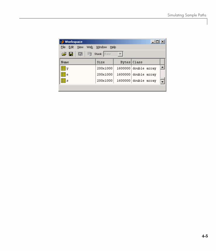
Simulating Sample Paths
4-5
4 Simulation
4-6
Presample DataBecause the mean equation and the variance equations can be recursive in nature, they require initial, or presample, data to initiate the simulation. You can use one of these methods.
• “Automatically Generated Presample Data” on page 4-6
• “User-Specified Presample Data” on page 4-10
Automatically Generated Presample DataWhen you allow garchsim to automatically generate the required initial data,
• garchsim performs independent path simulation. That is, all simulated realizations are unique in that they evolve independently and share no common presample conditioning data.
• garchsim generates the presample data in a way that minimizes transient effects in the output processes.
Automatic Minimization of Transient Effectsgarchsim generates output processes in (approximately) steady state by attempting to eliminate transients in the data it simulates. garchsim first estimates the number of observations needed for the transients to decay to some arbitrarily small value, subject to a 10000 observation maximum. It then generates a number of observations equal to the sum of this estimated value and the number of observations you request. garchsim then ignores the earlier estimated number of initial observations needed for the transients to decay sufficiently, and returns only the requested number of later observations.
To do this, garchsim interprets a GARCH(P,Q) or GJR(P,Q) conditional variance process as an ARMA(max(P,Q),P) model for the squared innovations, and interprets an EGARCH(P,Q) process as an ARMA(P,Q) model for the log of the conditional variance. (See, for example, Bollerslev [4], p.310.) garchsim then interprets the ARMA model as the correlated output of a linear filter and estimates its impulse response by finding the magnitude of the largest eigenvalue of its autoregressive polynomial. Based on this eigenvalue, garchsim estimates the number of observations, subject to a 10000 maximum, needed for the magnitude of the impulse response, which begins at 1, to decay below the default response tolerance 0.01 (i.e., 1 percent). If the conditional mean has an ARMA(R,M) component, then garchsim also estimates the

Presample Data
4-7
number of observations needed for the impulse response to decay below the response tolerance. This number is also subject to a 10000 maximum.
The effect of transients in the simulation process parallels that in the estimation, or inference, process. “Presample Data and Transient Effects” on page 5-23 provides an example of transient effects in the estimation process.
Specifying a Scalar Response ToleranceIf you want to use a response tolerance other than the default 0.01, you can specify it via the Tolerance argument. This example compares simulated observations generated using the default response tolerance, 0.01, and a larger tolerance 0.05. It uses the model from “Simulating Sample Paths” on page 4-2.
Start by simulating a single path of 200 observations using the default tolerance 0.01.
[e1,s1,y1] = garchsim(coeff,200)garchplot(e1,s1,y1)
0 20 40 60 80 100 120 140 160 180 200−0.02
−0.01
0
0.01Innovations
Inno
vatio
n
0 20 40 60 80 100 120 140 160 180 2002
4
6
8x 10
−3 Conditional Standard Deviations
Sta
ndar
d D
evia
tion
0 20 40 60 80 100 120 140 160 180 200−0.02
−0.01
0
0.01Returns
Ret
urn

4 Simulation
4-8
Now, simulate another path of 200 observations, but specify the scalar Tolerance argument as 0.05.
[e5,s5,y5] = garchsim(coeff,200,[],[],[],0.05)garchplot(e5,s5,y5)
The observations generated using the 0.05 response tolerance are the same as those generated for the default 0.01 tolerance, but shifted to the right. This is because it took fewer observations for the magnitude of the impulse response to decay below the larger 0.05 tolerance. If you make the Tolerance smaller than 0.01, note that garchsim might have to generate more observations and could conceivably reach the 10000 observation transient decay period maximum or run out of memory.
Storage ConsiderationsDepending on the values of the parameters in the simulated conditional mean and variance models, you may need long presample periods for the transients
0 20 40 60 80 100 120 140 160 180 200−0.02
−0.01
0
0.01Innovations
Inno
vatio
n
0 20 40 60 80 100 120 140 160 180 2002
4
6
8x 10
−3 Conditional Standard Deviations
Sta
ndar
d D
evia
tion
0 20 40 60 80 100 120 140 160 180 200−0.02
−0.01
0
0.01Returns
Ret
urn

Presample Data
4-9
to die out. Although the simulation outputs may be relatively small matrices, the initial computation of these transients can result in a large memory burden and seriously impact performance. Because of this, garchsim imposes a maximum of 10000 observations to the transient decay period of each realization. The example in “Simulating Multiple Paths” on page 4-4, which simulates three 200-by-1000 element arrays, requires intermediate storage for far more than 200 observations.
Other Ways to Minimize Transient EffectsIf you suspect that transients persist in the simulated data garchsim returns, you can use one of these methods to minimize their effect:
• “Oversampling” on page 4-9
• “Recycling Outputs” on page 4-10
Oversampling. Generate samples that are larger than you need, and delete observations from the beginning of each output series. For example, suppose you would like to simulate 10 independent paths of 1000 observations each for
, , and starting from a known scalar random number seed (12345).
Start by generating 1200 observations. garchsim generates sufficient presample data so that it can ignore initial samples that might be affected by transients. It then returns only the requested 1200 later observations.
[e,s,y] = garchsim(coeff,1200,10,12345);
εt{ } σt{ } yt{ }

4 Simulation
4-10
Further minimize the effect of transients by retaining only the last 1000 observations of interest.
e = e(end-999:end,:);s = s(end-999:end,:);y = y(end-999:end,:);
Note The example above also illustrates how to specify a scalar random number generator “seed.” This use corresponds to the rand and randn syntaxes, rand('state',j) and randn('state',j). If you do not specify a seed, the default is 0, the random number generator initial state.
Recycling Outputs. Start by simulating the desired number of observations without explicitly providing presample data i.e., let garchsim automatically generate the presample data. Then simulate again, using the simulated observations as the presample data. You can repeat this process until you are satisfied that transient effects have been sufficiently eliminated. See “User-Specified Presample Data” on page 4-10 for information about supplying presample data.
User-Specified Presample DataUse the time-series input arrays PreInnovations, PreSigmas, and PreSeries to explicitly specify all required presample data. These presample arrays are associated with the garchsim outputs Innovations, Sigmas, and Series,

Presample Data
4-11
respectively. When specified, garchsim uses these presample arrays to initiate the filtering process and form the conditioning set upon which the simulated realizations are based.
The PreInnovations, PreSigmas, and PreSeries arrays, as well as their associated outputs, are column-oriented arrays in which each column is associated with a distinct realization, or sample path. The first row of each array stores the oldest data and the last row the most recent.
Note that you can specify PreInnovations, PreSigmas, and PreSeries as matrices (i.e., with multiple columns), or as single-column vectors. In either case, the following table summarizes the minimum number of rows required to successfully initiate the simulation process.
If you specify PreInnovations, PreSigmas, and PreSeries as matrices, garchsim uses each column to initiate simulation of the corresponding column of the Innovations, Sigmas, and Series outputs. Each of the presample inputs must have NUMPATHS columns.
If you specify PreInnovations, PreSigmas, and PreSeries as column vectors, and NUMPATHS is greater than 1, garchsim performs dependent path simulation. That is, garchsim applies the same vector to each column of the corresponding Innovations, Sigmas, and Series outputs. All simulated sample paths share a common conditioning set. Although all realizations evolve independently, they share common presample conditioning data. Dependent path simulation enables the simulated sample paths to evolve from a common starting point, and allows Monte Carlo simulation of forecasts and forecast error distributions. See “Advanced Example” on page 9-1.
If you specify at least one set, but fewer than three sets, of presample data, garchsim does not attempt to derive presample observations for those you omit.
Minimum Number of Rows
garchsim Input Argument
GARCH(P,Q), GJR(P,Q)
EGARCH(P,Q)
PreInnovations max(M,Q) max(M,Q)
PreSigmas P max(P,Q)
PreSeries R R

4 Simulation
4-12
If you specify your own presample data, you must specify all that are necessary for the specified conditional mean and variance models. See the example “Specifying Presample Data” on page 5-19.
5
Estimation
“Estimation” includes these sections:
Maximum Likelihood Estimation (p. 5-2)
Explains how the estimation engine, garchfit, uses maximum likelihood to estimate the parameters needed to fit the specified models to a given univariate return series.
Initial Parameter Estimates (p. 5-4)
Describes the use of both user-supplied and automatically generated initial parameter estimates. It also explains how garchfit uses parameter bounds to provide stability in the optimization process.
Presample Observations (p. 5-11)
Explains how garchfit calculates automatically generated presample data for the conditional mean model and for each of the supported conditional variance models. It also explains how to specify your own presample data.
Termination Criteria and Optimization Results (p. 5-13)
Discusses the optimization parameters that enable you to influence the optimization process.
Examples (p. 5-19) Illustrates presample data, transient effects, and lower bound constraints. It also offers an alternative technique for estimating ARMA(R,M) parameters.

5 Estimation
5-2
Maximum Likelihood EstimationGiven models for the conditional mean and variance (see “Conditional Mean and Variance Models” on page 2-6), and an observed univariate return series, the estimation engine garchfit infers the innovations (i.e., residuals) from the return series, and estimates, by maximum likelihood, the parameters needed to fit the specified models to the return series.
garchfit calls the Optimization Toolbox function fmincon to perform constrained optimization of a scalar function of several variables, i.e., the log-likelihood function, given a vector of initial parameter estimates (see “Initial Parameter Estimates” on page 5-4). This is generally referred to as constrained nonlinear optimization or nonlinear programming. In turn, fmincon calls the appropriate log-likelihood objective function to estimate the model parameters via maximum likelihood estimation (MLE). The chosen log-likelihood objective function proceeds in three steps:
1 Given the vector of current parameter values and the observed data Series, the log-likelihood function infers the process innovations (i.e., residuals) by inverse filtering. This inference, or inverse filtering, operation rearranges the conditional mean equation to solve for the current innovation, :
This equation is a whitening filter, transforming a (possibly) correlated process into an uncorrelated white noise process .
2 The log-likelihood function then uses the inferred innovations to infer the corresponding conditional variances via recursive substitution into the model-dependent conditional variance equations (Eq. (2-4), Eq. (2-5), Eq. (2-6)) above.
3 Finally, the function uses the inferred innovations and conditional variances to evaluate the appropriate log-likelihood objective function. If is Gaussian, the log-likelihood function is
εt
εt C– yt φiyt i–i 1=
R
∑– θjεt j–
j 1=
M
∑– βkX t k,( )k 1=
Nx
∑–+=
yt εt
εt
σt2
εt

Maximum Likelihood Estimation
5-3
(5-1)
If is Student’s t, the log-likelihood function is
(5-2)
where is the sample size, i.e., the number of rows in the series . The degrees of freedom must be greater than 2.
Notice that the conditional mean equation (Eq. (2-2)) and the conditional variance equations (Eq. (2-4), Eq. (2-5), and Eq. (2-6)) are recursive and, in general, require presample observations to initiate the inverse filtering. For this reason, the objective functions shown above are referred to as conditional log-likelihood functions. That is, evaluation of the log-likelihood function is conditioned, or based, on a set of presample observations. The methods used to specify these presample observations are discussed in “Presample Observations” on page 5-11.
The iterative numerical optimization repeats the three steps described above until suitable termination criteria are reached. See “Termination Criteria and Optimization Results” on page 5-13 for details.
LLF T2----– log 2π( ) 1
2--- logσt
2
t 1=
T
∑–12--- εt
2 σt2
⁄
t 1=
T
∑–=
εt
LLF Tlog Γ v 1+( ) 2⁄[ ]
π1 2⁄ Γ v 2⁄( )--------------------------------- v 2–( ) 1 2⁄–
1
2--- logσt
2
t 1=
T
∑–=
v 1+2
------------ log 1εt
2
σt2
v 2–( )------------------------+
t 1=
T
∑–
T yt{ }v

5 Estimation
5-4
Initial Parameter EstimatesThe constrained nonlinear optimizer, fmincon, requires a vector of initial parameter estimates. Although garchfit computes initial parameter estimates if you provide none, at times it may be helpful to compute and specify your own initial guesses to avoid convergence problems.
This section discusses
• “User-Specified Initial Estimates” on page 5-4
• “Automatically Generated Initial Estimates” on page 5-5
• “Parameter Bounds” on page 5-9
User-Specified Initial EstimatesYou can specify complete initial estimates for either or both the conditional mean equation and the conditional variance equation.
For the conditional mean estimates to be complete, you must specify the C, AR, and MA parameters, consistent with the orders you specified for R and M; i.e., the length of AR must be R, and the length of MA must be M. You must also specify the Regress parameter if you provide a regression matrix . C, AR, MA, and Regress correspond respectively to , , , and in Eq. (2-2).
Note To remove the constant from the conditional mean model, i.e., to fix C = 0 without providing initial parameter estimates for the remaining parameters, set C = NaN (Not-a-Number). In this case, the value of FixC has no effect.
For the conditional variance estimates to be complete, you must specify the K, GARCH, and ARCH specification structure parameters for all conditional variance models, consistent with the orders you specified for P and Q; i.e., the length of GARCH must be P, and the length of ARCH must be Q. You must also specify the Leverage parameter for GJR and EGARCH conditional variance models. The parameters K, GARCH, ARCH, and Leverage correspond respectively to , ,
,and in Eq. (2-4), Eq. (2-5), and Eq. (2-6).
You can use garchset to create the necessary specification structure, Spec, or you can modify the Coeff structure returned by a previous call to garchfit.
XC φj θi βk
C
κ GiAj Lj

Initial Parameter Estimates
5-5
If you provide initial parameter estimates for a model equation, you must provide all the estimated constants and coefficients consistent with the specified model orders. For example, for an ARMA(2,2) model with no regression matrix, you must specify the parameters C, AR, and MA. If you specify only MA, the specification is incomplete, and garchfit ignores the MA you specified and automatically generates all the requisite initial estimates.
The following specification structure provides C and AR as initial parameter estimates, but does not provide MA, even though M = 1. In this case, garchfit ignores the C and AR fields, computes initial parameter estimates, and overwrites any existing parameters in the incomplete conditional mean specification.
spec = garchset('R',1,'M',1,'C',0,'AR',0.5,... 'P',1,'Q',1,'K',0.0005,'GARCH',0.8,'ARCH',0.1)spec =
Comment: 'Mean: ARMAX(1,1,?); Variance: GARCH(1,1)' Distribution: 'Gaussian' R: 1 M: 1 C: 0 AR: 0.5000 MA: [] VarianceModel: 'GARCH' P: 1 Q: 1 K: 5.0000e-004 GARCH: 0.8000 ARCH: 0.1000
However, since the structure explicitly sets all fields in the conditional variance model, garchfit uses the specified values of K, GARCH, and ARCH as initial estimates subject to further refinement.
Automatically Generated Initial EstimatesIf you do not provide initial coefficient estimates for a conditional mean or variance model, or if the estimates you provide are incomplete, garchfit automatically generates initial estimates. It first estimates the conditional mean parameters, if necessary, then estimates the conditional variance

5 Estimation
5-6
parameters, if necessary. Again, note that garchfit ignores any incomplete initial estimates. garchfit estimates initial conditional mean parameters using standard statistical time-series techniques, dependent upon the parametric form of the conditional mean equation.
• “Conditional Mean Models Without a Regression Component” on page 5-6
• “Conditional Mean Models with a Regression Component” on page 5-6
• “Conditional Variance Models” on page 5-7
Conditional Mean Models Without a Regression Component
ARMA Models. Initial parameter estimates of general ARMA(R,M) conditional mean models are estimated by the three-step method outlined in Box, Jenkins, and Reinsel [8], Appendix A6.2.
1 garchfit estimates the autoregressive coefficients, , by computing the sample autocovariance matrix and solving the Yule-Walker equations.
2 Using these estimated coefficients, garchfit filters the observed Series to obtain a pure moving average process.
3 garchfit computes the autocovariance sequence of the moving average process, and uses it to iteratively estimate the moving average coefficients, . This last step also provides an estimate of the unconditional variance of the innovations.
Conditional Mean Models with a Regression Component
ARX Models (No Moving Average Terms Allowed). Initial estimates of the autoregressive coefficients, , and the regression coefficients, , of the explanatory data matrix, , are generated by ordinary least squares regression.
See “Regression Components in Conditional Mean Models” on page 7-1 for more information.
ARMAX Models (Moving Average Terms Included). Initial parameter estimation of the general ARMAX conditional mean models requires two steps:
1 garchfit estimates an ARX model by ordinary least squares.
φj
θi
φj βkX

Initial Parameter Estimates
5-7
2 garchfit estimates an MA(M) = ARMA(0,M) model as outlined in “Conditional Mean Models Without a Regression Component” on page 5-6.
Conditional Variance ModelsAs opposed to conditional mean parameters, initial estimates of conditional variance parameters are based on empirical analysis of financial time series, and are thus ad hoc. The approach is dependent upon the conditional variance model you select.
GARCH(P,Q) Models. For GARCH models, garchfit assumes that the sum of the and the is close to 1. Specifically, for a
general GARCH(P,Q) model (Eq. (2-4)), garchfit assumes that
If (i.e., lagged conditional variances are included), then garchfit equally allocates 0.85 out of the available 0.90 to the GARCH coefficients, and allocates the remaining 0.05 equally among the ARCH coefficients. specifies an ARCH(Q) model in which garchfit allocates 0.90 equally to the ARCH terms. Some examples will clarify the approach.
The GARCH(1,1) model is by far the most common, and initial estimates are expressed as follows:
A GARCH(2,1) model would be initially expressed as
An ARCH(1) model would be initially expressed as
An ARCH(2) model would be initially expressed as
Finally, garchfit estimates the constant of the conditional variance model by first estimating the unconditional, or time-independent, variance of .
Gi i 1 … P, ,=( ), Aj j 1 … Q, ,=( ),
G1 … GP A1 … AQ+ + + + + 0.9=
P 0>P
Q P 0=Q
σt2 κ 0.85σt 1–
20.05εt 1–
2+ +=
σt2 κ 0.425σt 1–
20.425σt 2–
20.05εt 1–
2+ + +=
σt2 κ 0.9εt 1–
2+=
σt2 κ 0.45εt 1–
20.45εt 2–
2+ +=
κεt{ }

5 Estimation
5-8
In terms of the parameters this can also be expressed as
and so
GJR(P,Q) Models. garchfit treats a GJR(P,Q) model, described in Eq. (2-5), as a straightforward extension of an equivalent GARCH(P,Q) model with zero leverage terms. Thus, initial parameter estimates of GJR models are identical to those of equivalent order GARCH models (see “GARCH(P,Q) Models” on page 5-7), with the additional assumption that all leverage terms are zero,
EGARCH(P,Q) Models. For EGARCH models garchfit assumes that the sum of the is 0.9, and the sum of the is 0.2. Specifically, for a general EGARCH(P,Q) model (Eq. (2-6)), garchfit assumes that
and
If , i.e., lagged conditional variances are included, then garchfit equally allocates the available weight of 0.9 to the GARCH coefficients, and equally allocates the available weight of 0.2 to the ARCH coefficients.
σ2 1T---- εt
2
t 1=
T
∑=
σ2 κ
1 Gi
i 1=
P
∑ Aj
j 1=
Q
∑––
-------------------------------------------------κ
1 0.85 0.05+( )–-------------------------------------------= =
κ σ21 0.85 0.05+( )–( )=
0.1σ2=
Li 0= 1 i Q≤ ≤
Gi i 1 … P, ,=( ), Aj j 1 … Q, ,=( ),
G1 G2 … GP+ + + 0.9=
A1 A2 … AQ+ + + 0.2=
Li 0= 1 i Q≤ ≤
P 0>PQ

Initial Parameter Estimates
5-9
Recall that, in EGARCH models, the standardized innovation, , serves as the forcing variable for both the conditional variance and the error, so that volatility clustering (i.e., persistence) is entirely captured by the terms. In other words, EGARCH models make no allowance for the relationship between the and coefficients regarding initial parameter estimates. Because of this, EGARCH(0,Q) models ignore the persistence effect commonly associated with financial returns and are somewhat unusual. Some examples clarify the approach.
The EGARCH(1,1) model is by far the most common, and initial estimates are expressed as:
Initial estimates for an EGARCH(2,2) model are expressed as
An EGARCH(0,1) model would be initially expressed as
As you can see, initial parameter estimates for EGARCH models are most effective when .
Finally, you can estimate the constant of an EGARCH conditional variance model by noting the approximate relationship between the unconditional variance of the innovations process, , and the parameters of an EGARCH(1,1) model:
Parameter Boundsgarchfit bounds some model parameters to provide stability in the optimization process. See the example “Active Lower Bound Constraint” on
zt
Gi
Gi Aj
logσt2 κ 0.9logσt 1–
20.2 zt 1– E zt 1–( )–[ ]+ +=
logσt2 κ 0.45logσt 1–
20.45logσt 2–
2++ +=
0.1 zt 1– E zt 1–( )–[ ] 0.1 zt 2– E zt 2–( )–[ ]+
logσt2 κ 0.2 zt 1– E zt 1–( )–[ ]+=
P 0>
κ
σ2Gi
κ 1 G1–( ) logσ2=
1 0.9–( ) logσ2=
0.1 logσ2=

5 Estimation
5-10
page 5-28 for more information on overriding these bounds in the unlikely event they become active.
Conditional Mean ModelFor the conditional mean model, Eq. (2-2), garchfit bounds the conditional mean constant and the conditional mean regression coefficients , if any, in the interval [-10,10]. However, if the coefficient estimates, whether provided by the user or automatically generated by garchfit, are outside this interval, garchfit sets the appropriate lower or upper bound equal to the estimated coefficient.
GARCH(P,Q) and GJR(P,Q) Conditional Variance ModelsFor GARCH(P,Q) and GJR(P,Q) conditional variance models, Eq. (2-3) and Eq. (2-4), garchfit uses 5 as an upper bound for the conditional variance constant . However, if the initial estimate is greater than 5, garchfit uses the estimated value as the upper bound.
EGARCH(P,Q) Conditional Variance ModelFor EGARCH(P,Q) conditional variance models, Eq. (2-5), garchfit places arbitrary bounds on the conditional variance constant , such that . However, if the magnitude of the initial estimate is greater than 5, garchfit adjusts the bounds accordingly.
C βk
κ
κ 5– κ 5≤ ≤

Presample Observations
5-11
Presample ObservationsYou can explicitly specify all required presample data, or you can allow garchfit to automatically generate the necessary presample data. “Maximum Likelihood Estimation” on page 5-2 discusses presample data required to initiate the inverse filtering and evaluate the conditional log-likelihood objective function.
This section discusses
• “User-Specified Presample Observations” on page 5-11
• “Automatically Generated Presample Observations” on page 5-11
User-Specified Presample ObservationsUse the time-series column vector inputs PreInnovations, PreSigmas, and PreSeries to explicitly specify all required presample data.The following table summarizes the minimum number of rows required to successfully initiate the optimization process.
If you specify at least one set, but fewer than three sets, of presample data, garchfit does not attempt to derive presample observations for those you omit. If you specify your own presample data, you must specify all that are necessary for the specified conditional mean and variance models. See the example “Specifying Presample Data” on page 5-19.
Automatically Generated Presample ObservationsIf you do not specify any presample data, garchfit automatically generates the required presample data.
Minimum Number of Rows
garchfit Input Argument
GARCH(P,Q), GJR(P,Q)
EGARCH(P,Q)
PreInnovations max(M,Q) max(M,Q)
PreSigmas P max(P,Q)
PreSeries R R

5 Estimation
5-12
Conditional Mean ModelsFor conditional mean models with an autoregressive component, garchfit assigns the R required presample observations (i.e., PreSeries) of the sample mean of Series. For models with a moving-average component, it sets the M required presample observations (i.e., PreInnovations) of to their expected value of zero. With this presample data, garchfit can infer the entire sequence of innovations for any general ARMAX conditional mean model regardless of the conditional variance model you select.
garchfit attempts to eliminate the effect of transients in the presample data it generates. This effect parallels that in the simulation process described in “Automatically Generated Presample Data” on page 4-6. The example “Presample Data and Transient Effects” on page 5-23 provides an example of transient effects in the estimation process.
GARCH(P,Q) ModelsOnce garchfit computes the innovations, it assigns the sample mean of the squared innovations
to the P and Q required presample observations of and , respectively. See Hamilton [18] and Bollerslev [4].
GJR(P,Q) Modelsgarchfit also assigns the average squared innovation to all required presample observations of and . In addition, garchfit weights the Q presample observations of associated with the leverage terms by 0.5 (i.e., the probability of a negative past residual).
EGARCH(P,Q) Modelsgarchfit also assigns the average squared innovation to all P presample observations of . In addition, it sets all Q presample observations of the standardized innovations to zero and to the mean absolute deviation. This has the effect of setting all Q presample ARCH and leverage terms to zero.
yt
εt
σ2 1T---- εt
2
t 1=
T
∑=
σt2 εt
2
σt2 εt
2
εt2
σt2
zt εt σt⁄( )= zt εt σt⁄( )=

Termination Criteria and Optimization Results
5-13
Termination Criteria and Optimization ResultsThere are several fields in the specification structure that allow you to influence the optimization process. In order of importance, these are
This section discusses
• “MaxIter and MaxFunEvals” on page 5-13
• “TolCon, TolFun, and TolX” on page 5-14
• “Convergence” on page 5-14
• “Optimization Results” on page 5-15
• “Constraint Violation Tolerance” on page 5-16
See the Optimization Toolbox documentation and the garchset function for additional information about these parameters.
MaxIter and MaxFunEvalsMaxIter is the maximum number of iterations allowed in the estimation process. Each iteration involves an optimization phase in which garchfit suitably modifies calculations such as line search, gradient, and step size. The default value of MaxIter is 400. Although an estimation rarely exceeds MaxIter, you can increase the value if you suspect that the estimation terminated prematurely.
MaxFunEvals, a field closely related to MaxIter, specifies the maximum number of log-likelihood objective function evaluations. The default value is 100 times the number of parameters estimated in the model. For example, the default model has four parameters, so the default value of MaxFunEvals for the default model is 400. When the estimation process terminates prematurely, it is usually because MaxFunEvals, rather than MaxIter, is exceeded. You can
TolCon Termination tolerance on the constraint violation
TolFun Termination tolerance on the function value
TolX Termination tolerance on the parameter estimates
MaxFunEvals Maximum number of function evaluations allowed
MaxIter Maximum number of iterations allowed

5 Estimation
5-14
increase MaxFunEvals if you suspect that the estimation terminated prematurely.
The fields MaxFunEvals and MaxIter are purely mechanical in nature. Although you may encounter situations in which MaxFunEvals or MaxIter is reached, this is rather uncommon. Increasing MaxFunEvals or MaxIter may allow successful convergence, but reaching MaxFunEvals or MaxIter is usually an indication that your model poorly describes the data; in particular, it often indicates that the model is too complicated. Finally, although MaxFunEvals and MaxIter can cause the function to stop before a solution is found, they do not affect the solution once it is found.
TolCon, TolFun, and TolXThe fields TolCon, TolFun, and TolX are tolerance-related parameters that directly influence how and when convergence is achieved, and can also affect the solution.
TolCon is the termination tolerance placed on constraint violations, and represents the maximum value by which parameter estimates can violate a constraint and still allow successful convergence. See “Conditional Mean and Variance Models” on page 2-6 for information about these constraints.
TolFun is the termination tolerance placed on the log-likelihood objective function. Successful convergence occurs when the log-likelihood function value changes by less than TolFun. See “Optimization Results” on page 5-15 for more information.
TolX is the termination tolerance placed on the estimated parameter values. Similar to TolFun, successful convergence occurs when the parameter values change by less than TolX. See “Optimization Results” on page 5-15 for more information.
ConvergenceTolFun, and TolX have the same default value, 1e-006. The TolCon default is 1e-007. If you experience extreme difficulty in convergence (e.g., the estimation shows little or no progress, or shows progress but stops early), then increasing one or more of these parameter values, for example, from 1e-006 to 1e-004, may allow the estimation to converge. If the estimation appears to converge to a suboptimal solution, then decreasing one or more of these

Termination Criteria and Optimization Results
5-15
parameter values (e.g., from 1e-006 to 1e-007) may provide more accurate parameter estimates.
Note You can avoid many convergence difficulties by performing a prefit analysis. “Analysis and Estimation Example Using the Default Model” on page 2-15 describes graphical techniques, e.g., plotting the return series, and examining the ACF and PACF. It also discusses some preliminary tests, including Engle’s ARCH test and the Q-test.
“Model Selection and Analysis” on page 8-1 discusses other tests to help you determine the appropriateness of a specific GARCH model. It also explains how equality constraints can help you assess parameter significance. “GARCH Limitations” on page 1-3 mentions some limitations of GARCH models that could affect convergence.
Optimization ResultsIn contrast to MaxIter and MaxFunEvals, the tolerance fields TolCon, TolFun, and TolX do affect the optimization results (see “TolCon, TolFun, and TolX” on page 5-14). At successful termination, assuming iterative display is selected, you will typically see one of the following messages:
Optimization terminated successfully:Magnitude of directional derivative in search directionless than 2*options.TolFun and maximum constraint violation is less than options.TolCon
Optimization terminated successfully:Search direction less than 2*options.TolX andmaximum constraint violation is less than options.TolCon
Optimization terminated successfully:First-order optimality measure less than options.TolFun andmaximum constraint violation is less than options.TolCon
Increasing TolFun or TolX from the default of 1e-6 to, for example, 1e-5, relaxes one or both of the first two termination criteria, often resulting in a slightly less accurate solution. Similarly, decreasing TolFun or TolX to, for

5 Estimation
5-16
example, 1e-7, restricts one or both of the first two termination criteria, often resulting in a slightly more accurate solution, but may also require more iterations. However, experience has shown that the default value of 1e-6 for TolFun and TolX is almost always sufficient, and changing the value is unlikely to significantly affect the estimation results for GARCH modeling. For this reason, it is recommended that you accept the default value for TolFun and TolX.
The GARCH Toolbox default value of TolCon is 1e-7, and changing the value of TolCon can significantly affect the solution in situations in which a constraint is active. For the GARCH Toolbox, from a practical standpoint, TolCon is the most important optimization-related field, and an additional discussion of its significance and use is helpful.
Whenever garchfit actively imposes parameter constraints (other than user-specified equality constraints) during the estimation process, the statistical results based on the maximum likelihood parameter estimates are invalid. (See Hamilton [18], page 142.) This is because statistical inference relies on the log-likelihood function’s being approximately quadratic in the neighborhood of the maximum likelihood parameter estimates. This cannot be the case when the estimates fail to fall in the interior of the parameter space.
Constraint Violation ToleranceAt each step in the optimization process, garchfit evaluates the constraints described in “Conditional Mean and Variance Models” on page 2-6 against the current intermediate solution vector. For each user-specified equality constraint, it determines whether or not there is a violation whose absolute value is greater than TolCon. For each inequality constraint (including lower and upper bounds), it determines whether or not the inequality is violated by more than TolCon. If either TolFun or TolX exit condition is satisfied, and if the maximum of any violations is less than TolCon, then the optimization terminates successfully. (See “TolCon, TolFun, and TolX” on page 5-14.)
Strict Inequality ConstraintsFor the Optimization Toolbox, the numerical optimizer, fmincon, defines inequality constraints as a less than or equal to condition. However, many GARCH Toolbox inequality constraints are strict inequalities that specifically exclude exact equality. For this reason the GARCH Toolbox interprets TolCon differently from the Optimization Toolbox.

Termination Criteria and Optimization Results
5-17
While TolCon applies to both strict inequalities and those that are not strict, garchfit provides special handling for strict inequalities. Specifically, garchfit associates each strict inequality constraint with its theoretical bound, or limit. However, to avoid the possibility of violating strict inequality constraints, garchfit defines the actual bound for each such constraint as the theoretical bound offset by 2*TolCon. Since the optimization can successfully terminate if the actual bound is violated by as much as TolCon, the end result is that any given strict inequality constraint is allowed to approach its theoretical bound to within TolCon.
Single Parameter Strict Inequality ConstraintsAlthough it is possible for an estimate of a strict inequality constraint that involves a single parameter to terminate a distance TolCon from its theoretical bound, experience has shown that this is unlikely. Examples of such constraints are the conditional variance constant for the GARCH(P,Q) and GJR(P,Q) models, and the degrees of freedom for the Student’s t distribution. Typically, when the lower or upper bound of such a single-parameter inequality constraint is active, the estimate remains 2*TolCon from the bound.
Note that even though the possibility is remote that an estimate of a single parameter constraint will terminate a distance TolCon from its theoretical bound, the garchfit approach for handling strict inequalities still allows for it.
As an illustration, assume TolCon = 1e-7 (i.e., the GARCH Toolbox default value), and consider the default GARCH(1,1) model:
with constraints
When the lower bound constraint is active, the estimated value of is typically .
κ 0>v 2>
yt C εt+=
σt2
κ G1σt 1–2
A1εt 1–2
+ +=
κ 0>
G1 A1+ 1<
G1 0≥
A1 0≥
κ 0> κκ 2e 7– 2*TolCon= =

5 Estimation
5-18
Relaxing Constraint Tolerance LimitsExperience has shown that relaxing TolCon is more apt to remove an active constraint in some cases than in others. For inequality constraints with a single parameter, such as for the GARCH(P,Q) and GJR(P,Q) models and
for the Student’s t distribution, decreasing TolCon may relax the constraint such that it is no longer active. The example “Active Lower Bound Constraint” on page 5-28 explains how to identify such a condition by examining the summary output structure.
This is not generally true for linear inequality constraints with multiple parameters. An example is . When this constraint is active, the estimated values of and are typically such that
. Decreasing TolCon to, say, 1e-8 allows to approach 1.0 a bit more closely, but the linear inequality constraint
is likely to remain active.
κ 0>v 2>
G1 A1+ 1<G1 A1
G1 A1+ 0.9999999 1.0 TolCon–= =G1 A1+

Examples
5-19
Examples• “Specifying Presample Data” on page 5-19
• “Presample Data and Transient Effects” on page 5-23
• “Alternative Technique for Estimating ARMA(R,M) Parameters” on page 5-27
• “Active Lower Bound Constraint” on page 5-28
• “Determining Convergence Status” on page 5-31
Specifying Presample DataThis example shows you how to specify your own presample data to initiate the estimation process. It highlights the formal column-oriented nature of the presample time-series inputs.
1 Load the Nasdaq data set and convert prices to returns.
load garchdatanasdaq = price2ret(NASDAQ);
Suppose, for example, that you want to segment the Nasdaq data in an effort to compare estimation results obtained from a relatively stable period to those from a period of relatively high volatility. If you examine the Nasdaq returns, there is a rather distinct increase in volatility starting, approximately, in December 1997. Roughly, this is the 2000th observation.
plot(nasdaq)axis([0 length(nasdaq) -0.15 0.15])set(gca,'XTick',[1 507 1014 1518 2025 2529 3027])set(gca,'XTickLabel',{'Jan 1990' 'Jan 1992' 'Jan 1994' ... 'Jan 1996' 'Jan 1998' 'Jan 2000' 'Jan 2002'})ylabel('Return')title('Daily Returns')

5 Estimation
5-20
2 For this example, create a specification structure to model the Nasdaq returns as an MA(1) process with GJR(1,1) residuals,
spec = garchset('VarianceModel','GJR','M',1,'P',1,'Q',1,... 'Display','off');
3 Estimate the parameters, standard errors, and inferred residuals and standard deviations using the first 2000 observations, allowing garchfit to automatically generate the necessary presample observations. Then display the estimated coefficients and errors.
[coeff,errors,LLF,eFit,sFit] = garchfit(spec,nasdaq(1:2000));garchdisp(coeff,errors)
Mean: ARMAX(0,1,0); Variance: GJR(1,1) Conditional Probability Distribution: Gaussian Number of Model Parameters Estimated: 6
Jan 1990 Jan 1992 Jan 1994 Jan 1996 Jan 1998 Jan 2000 Jan 2002
−0.1
−0.05
0
0.05
0.1
0.15
Ret
urn
Daily Returns
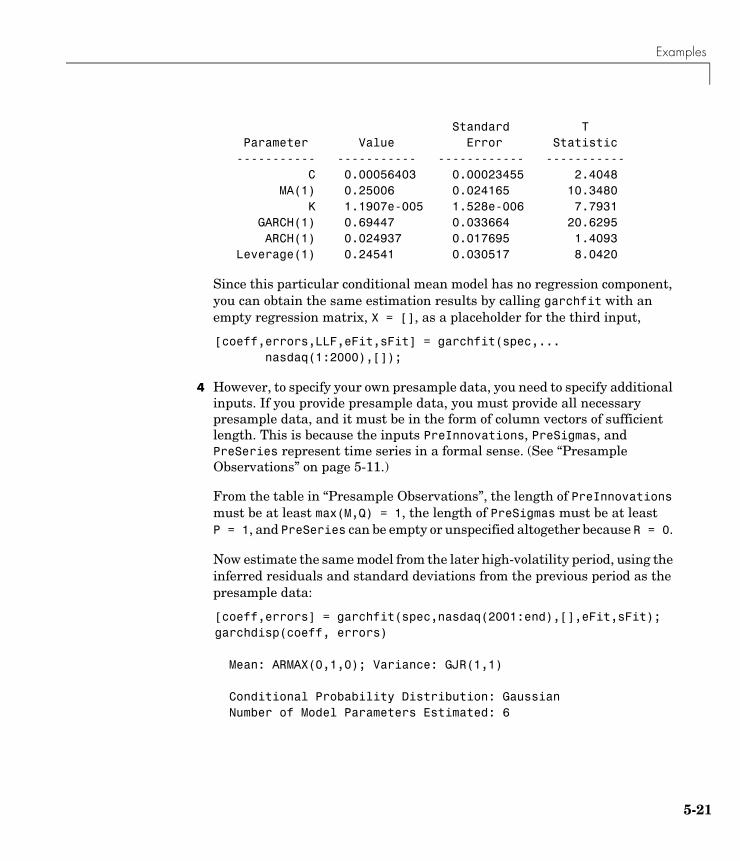
Examples
5-21
Standard T Parameter Value Error Statistic ----------- ----------- ------------ ----------- C 0.00056403 0.00023455 2.4048 MA(1) 0.25006 0.024165 10.3480 K 1.1907e-005 1.528e-006 7.7931 GARCH(1) 0.69447 0.033664 20.6295 ARCH(1) 0.024937 0.017695 1.4093 Leverage(1) 0.24541 0.030517 8.0420
Since this particular conditional mean model has no regression component, you can obtain the same estimation results by calling garchfit with an empty regression matrix, X = [], as a placeholder for the third input,
[coeff,errors,LLF,eFit,sFit] = garchfit(spec,... nasdaq(1:2000),[]);
4 However, to specify your own presample data, you need to specify additional inputs. If you provide presample data, you must provide all necessary presample data, and it must be in the form of column vectors of sufficient length. This is because the inputs PreInnovations, PreSigmas, and PreSeries represent time series in a formal sense. (See “Presample Observations” on page 5-11.)
From the table in “Presample Observations”, the length of PreInnovations must be at least max(M,Q) = 1, the length of PreSigmas must be at least P = 1, and PreSeries can be empty or unspecified altogether because R = 0.
Now estimate the same model from the later high-volatility period, using the inferred residuals and standard deviations from the previous period as the presample data:
[coeff,errors] = garchfit(spec,nasdaq(2001:end),[],eFit,sFit);garchdisp(coeff, errors)
Mean: ARMAX(0,1,0); Variance: GJR(1,1) Conditional Probability Distribution: Gaussian Number of Model Parameters Estimated: 6

5 Estimation
5-22
Standard T Parameter Value Error Statistic ----------- ----------- ------------ ----------- C 0.00065398 0.00060488 1.0812 MA(1) 0.012699 0.035131 0.3615 K 1.7845e-005 3.9153e-006 4.5578 GARCH(1) 0.85799 0.026246 32.6906 ARCH(1) 0.016147 0.022595 0.7146 Leverage(1) 0.17433 0.033234 5.2455
Comparing the estimation results from the two periods reveals a marked difference. Notice that the last input, PreSeries, is unnecessary and is left unspecified.
5 Since the example uses only the most recent observations of PreInnovations, PreSigmas, and PreSeries, any of the following calls to garchfit produce identical estimation results.
[coeff,errors] = garchfit(spec,nasdaq(2001:end),[],... eFit(end),sFit(end));
[coeff,errors] = garchfit(spec,nasdaq(2001:end),[],... eFit(end),sFit(end),nasdaq(1:2000));
[coeff,errors] = garchfit(spec,nasdaq(2001:end),... [],eFit,sFit,nasdaq(1999:2000));
The first equivalent call passes in the minimum required presample observations of past residuals and standard deviations, which in this case is the last inferred observation of each. The last two equivalent calls specify an unnecessary presample return series, which garchfit ignores.
If, for example, the original specification included an AR(2) model (i.e., = 2), then at least the last two Nasdaq returns are needed to initiate estimation. In this case, the last two calls to garchfit above would produce identical results for conditional mean models with AR components up to 2nd order.
R

Examples
5-23
Presample Data and Transient EffectsThis example simulates a return series, yTrue, then uses the inference function garchinfer to infer and from the simulated return series. First, the example uses automatically generated presample data to infer the approximate residuals and conditional standard deviation processes, and then uses explicitly specified presample data to infer the exact residuals and conditional standard deviation processes. The example finally compares the approximate conditional standard deviation processes with the exact conditional standard deviations processes to reveal the effect of transients in the approximate results. The effect of transients in the estimation, or inference, process parallels that in the simulations process described in “Automatically Generated Presample Data” on page 4-6.
Note This example uses garchinfer, rather than garchfit, to avoid introducing differences as a result of the optimization. While garchsim uses an ARMA model as a linear filter to transform an uncorrelated input innovations process into a correlated output returns process , garchinfer reverses this process (as does garchfit) by inferring innovations
and standard deviation processes from the observations in .
1 Specify a time series as an AR(2) conditional mean model and GARCH(1,2) conditional variance model. Note that this is an elaborate specification, typically unwarranted for a real-world financial time series, and is meant for illustration purposes only.
spec = garchset('C',0,'AR',[0.5 -0.8],'K',0.0002,... 'GARCH',0.8,'ARCH',[0.1 0.05])spec =
Comment: 'Mean: ARMAX(2,0,?); Variance: GARCH(1,2)' Distribution: 'Gaussian' R: 2 C: 0 AR: [0.5000 -0.8000] VarianceModel: 'GARCH' P: 1 Q: 2 K: 2.0000e-004
εt{ } σt{ }
εt{ } yt{ }
εt{ } σt{ } yt{ }

5 Estimation
5-24
GARCH: 0.8000 ARCH: [0.1000 0.0500]
2 Simulate 102 observations for each of 5 realizations and reserve the first 2 rows of observations for the presample data needed by garchinfer in step 4. From the table in “User-Specified Presample Data” on page 4-10, notice that the PreInnovations array must have at least max(M,Q) = 2 rows, PreSigmas must have at least P = 1 row, and PreSeries must have at least R = 2 rows.
[eTrue,sTrue,yTrue] = garchsim(spec,102,5);
3 Using observations 3 and beyond as the observed return series input, call garchinfer without any explicit presample data to infer the approximate residuals and conditional standard deviations based on the default, or automatic, presample data inference approach (see the garchfit and garchinfer functions for details).
[eApprox,sApprox] = garchinfer(spec,yTrue(3:end,:));
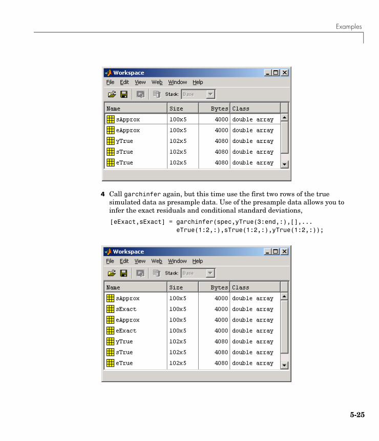
Examples
5-25
4 Call garchinfer again, but this time use the first two rows of the true simulated data as presample data. Use of the presample data allows you to infer the exact residuals and conditional standard deviations,
[eExact,sExact] = garchinfer(spec,yTrue(3:end,:),[],... eTrue(1:2,:),sTrue(1:2,:),yTrue(1:2,:));

5 Estimation
5-26
5 A graphical comparison of the first realization of the approximate and the exact inferred conditional standard deviations reveals the distinction between automatically generated and user-specified presample data.
plot(sApprox(:,1),'red')grid('on'),hold('on')plot(sExact(:,1),'blue')title('Approximate Versus Exact Inferred Standard Deviations')
Notice that the approximate and exact standard deviations are asymptotically identical. The only difference between the two curves is attributable to the transients induced by the default initial conditions.
In fact, if you were to plot the first realization of the original simulated conditional standard deviations, sTrue(3:end,1), on the current figure, it would lie completely on top of the blue curve.
Although the figure highlights the first realization of conditional standard deviations, the comparison holds for any realization, and for the inferred residuals as well.
0 20 40 60 80 1000.035
0.04
0.045
0.05
0.055
0.06
0.065
0.07
0.075
0.08Approximate Versus Exact Inferred Standard Deviations

Examples
5-27
Thus, this example reveals the link between simulation and inference: garchsim can be thought of as a correlation filter capable of processing multiple realizations simultaneously, and is the complement of garchinfer, which can be thought of as a whitening, or inverse, filter capable of processing multiple realizations simultaneously. Although the estimation engine garchfit is capable of processing only a single realization at a time, the transient effects highlighted in this example are exactly the same when applied to the estimation.
Alternative Technique for Estimating ARMA(R,M) ParametersThis example illustrates how to use the presample inputs PreInnovations and PreSeries to estimate the parameters of ARMA(R,M) models by a popular alternative technique. It assumes a simple constant variance model, and highlights the GARCH Toolbox as a general-purpose univariate time-series processor.
Default MethodAs mentioned above, estimation requires presample data to initiate the inverse filtering process. In the absence of any explicit presample data, garchfit assigns the required presample observations of , i.e., Series, the sample mean of Series. It also assigns the required presample observations of , i.e., the innovations, or residuals, their expected value of zero. This method then calculates the log-likelihood objective function value using all the available data in Series, and is the default method used by the GARCH Toolbox.
Alternative TechniqueAnother popular method also sets the required presample observations of the residuals, , to zero, but uses the first actual observations of Series as initial values. Thus, are used to initiate the inverse filter, and the log-likelihood objective function value is based on the remaining observations. See Hamilton [18], page 132, or Box, Jenkins, Reinsel [8], pages 236-237.
For example, assume you have some hypothetical time series, xyz, and you want to estimate an ARMA(R,M) model with constant conditional variances. Using the alternative presample method, you would exclude the first observations of xyz from the input Series, and reserve them for the input
R ytM εt
Mεt R
y1 y2 … yR, , ,{ }
R

5 Estimation
5-28
PreSeries. Specifically, you would set the input Series = xyz(R+1:end), PreInnovations = zeros(M,1), PreSigmas = [], and PreSeries = xyz(1:R).
Active Lower Bound ConstraintThis example illustrates an active lower bound constraint, , for the conditional variance constant . This constraint is required for GARCH and GJR variance models to ensure a positive conditional variance process. It also illustrates how to identify such active constraints, and what to do about this most commonly encountered active constraint. See “Termination Criteria and Optimization Results” on page 5-13.
1 Load the NYSE data set and convert prices to returns.
load garchdatanyse = price2ret(NYSE);
plot(nyse)axis([0 length(nyse) -0.08 0.06])set(gca,'XTick',[1 507 1014 1518 2025 2529 3027])set(gca,'XTickLabel',{'Jan 1990' 'Jan 1992' 'Jan 1994' ... 'Jan 1996' 'Jan 1998' 'Jan 2000' 'Jan 2002'})set(gca,'YTick',[-0.08:0.02:0.06])ylabel('Return')title('Daily Returns')
κ 0>κ

Examples
5-29
2 Estimate a default GARCH(1,1) model and print the estimation results. For this example, notice that TolCon = 1e-6, and iterative display is disabled for brevity.
spec = garchset('Display','off','P',1,'Q',1,'TolCon',1e-6);[coeff,errors,LLF,eFit,sFit,summary] = garchfit(spec,nyse);garchdisp(coeff,errors)
Mean: ARMAX(0,0,0); Variance: GARCH(1,1) Conditional Probability Distribution: Gaussian Number of Model Parameters Estimated: 4 Standard T Parameter Value Error Statistic ----------- ----------- ------------ ----------- C 0.00051941 0.00013701 3.7910 K 2e-006 2.8192e-007 7.0943
Jan 1990 Jan 1992 Jan 1994 Jan 1996 Jan 1998 Jan 2000 Jan 2002−0.08
−0.06
−0.04
−0.02
0
0.02
0.04
0.06
Ret
urn
Daily Returns

5 Estimation
5-30
GARCH(1) 0.87166 0.0095167 91.5925 ARCH(1) 0.10419 0.0073771 14.1238
3 Examination of these results reveals the estimated variance constant K = 2e-006 = 0 + 2*TolCon = 2*TolCon, i.e., is equal to the theoretical lower bound plus 2*TolCon. You can see this by printing the summary structure and looking at the constraints message field:
summary
summary = warning: 'No Warnings' converge: 'Function Converged to a Solution' constraints: 'Boundary Constraints Active: Standard Errors May Be Inaccurate' covMatrix: [4x4 double] iterations: 13 functionCalls: 115 lambda: [1x1 struct]
4 Print the lower and upper bound LaGrange multipliers and examine them for nonzero values:
[summary.lambda.lower summary.lambda.upper]
ans = 1.0e+006 *
0 0 7.3602 0 0 0 0 0
Notice that lower and upper bound LaGrange multipliers are ordered exactly as displayed by garchdisp. From this result, you can clearly see that the lower bound constraint is active.
5 Repeat the estimation with the default TolCon = 1e-7 and verify that the constraint is no longer active.
spec = garchset('Display','off','P',1,'Q',1);[coeff,errors,LLF,eFit,sFit,summary] = garchfit(spec,nyse);
κ
κ 0>

Examples
5-31
garchdisp(coeff,errors)
Mean: ARMAX(0,0,0); Variance: GARCH(1,1)
Conditional Probability Distribution: Gaussian Number of Model Parameters Estimated: 4
Standard T Parameter Value Error Statistic ----------- ----------- ------------ ----------- C 0.00049676 0.00013137 3.7813 K 8.9128e-007 1.5776e-007 5.6495 GARCH(1) 0.91088 0.0069142 131.7410 ARCH(1) 0.079942 0.0058319 13.7077
summary
summary = warning: 'No Warnings' converge: 'Function Converged to a Solution' constraints: 'No Boundary Constraints' covMatrix: [4x4 double] iterations: 21 functionCalls: 208 lambda: [1x1 struct]
[summary.lambda.lower summary.lambda.upper]
ans = 0 0 0 0 0 0 0 0
Determining Convergence StatusThere are two ways to determine whether an estimation achieves convergence. The first, and easiest, is to examine the optimization details of the estimation.

5 Estimation
5-32
By default, garchfit displays this information in the MATLAB command window. The second way to determine convergence status is to request the garchfit optional summary output.
To illustrate these methods, use the DEM2GBP (Deutschmark/British pound foreign exchange rate) data.
load garchdatadem2gbp = price2ret(DEM2GBP);[coeff,errors,LLF,eFit,sFit,summary] = garchfit(dem2gbp);
%%%%%%%%%%%%%%%%%%%%%%%%%%%%%%%%%%%%%%%%%%%%%%%%%%%%%%%%%%% Diagnostic Information
Number of variables: 4
Functions Objective: garchllfn Gradient: finite-differencing Hessian: finite-differencing (or Quasi-Newton) Nonlinear constraints: armanlc Gradient of nonlinear constraints: finite-differencing
Constraints Number of nonlinear inequality constraints: 0 Number of nonlinear equality constraints: 0 Number of linear inequality constraints: 1 Number of linear equality constraints: 0 Number of lower bound constraints: 4 Number of upper bound constraints: 4
Algorithm selected medium-scale
%%%%%%%%%%%%%%%%%%%%%%%%%%%%%%%%%%%%%%%%%%%%%%%%%%%%%%%%%%% End diagnostic information
max Directional First-orderIter F-count f(x) constraint Step-size derivative Optimality Procedure 1 28 -7916.01 -2.01e-006 7.63e-006 857 1.42e+005 2 36 -7959.65 -1.508e-006 0.25 389 9.8e+007 3 45 -7963.98 -3.113e-006 0.125 131 5.29e+006 4 52 -7965.59 -1.586e-006 0.5 55.9 4.45e+007

Examples
5-33
5 65 -7966.9 -1.574e-006 0.00781 101 1.46e+007 6 74 -7969.46 -2.201e-006 0.125 14.9 2.77e+007 7 83 -7973.56 -2.663e-006 0.125 36.6 1.45e+007 8 90 -7982.09 -1.332e-006 0.5 -6.39 5.59e+006 9 103 -7982.13 -1.399e-006 0.00781 6.49 1.32e+006 10 111 -7982.53 -1.049e-006 0.25 12.5 1.87e+007 11 120 -7982.56 -1.186e-006 0.125 3.72 3.8e+006 12 128 -7983.69 -1.11e-006 0.25 0.184 4.91e+006 13 134 -7983.91 -7.813e-007 1 0.732 1.22e+006 14 140 -7983.98 -9.265e-007 1 0.186 1.17e+006 15 146 -7984 -8.723e-007 1 0.0427 9.52e+005 16 154 -7984 -8.775e-007 0.25 0.0152 6.33e+005 17 160 -7984 -8.75e-007 1 0.00197 6.98e+005 18 166 -7984 -8.763e-007 1 0.000931 7.38e+005 19 173 -7984 -8.759e-007 0.5 0.000469 7.37e+005 20 179 -7984 -8.761e-007 1 0.00012 7.22e+005 21 199 -7984 -8.761e-007 -6.1e-005 0.0167 7.37e+005 Hessian modified twice22 213 -7984 -8.761e-007 0.00391 0.00582 7.26e+005 Hessian modified twiceOptimization terminated successfully: Search direction less than 2*options.TolX and maximum constraint violation is less than options.TolCon No Active Constraints
Notice that the optimization details indicate successful termination. Now, examine the summary output structure.
summary
summary = warning: 'No Warnings' converge: 'Function Converged to a Solution' constraints: 'No Boundary Constraints' covMatrix: [4x4 double] iterations: 22 functionCalls: 213 lambda: [1x1 struct]
The converge field indicates successful convergence. If the estimation failed to converge, the converge field would contain the message 'Function Did NOT Converge'. If the number of iterations or function evaluations exceeded its specified limits, the converge field would contain the message 'Maximum Function Evaluations or Iterations Reached'. The summary structure also contains fields that indicate the number of iterations (iterations) and log-likelihood function evaluations (functionCalls).

5 Estimation
5-34

6
Forecasting
“Forecasting” includes these sections:
Minimum Mean Square Error Forecasting (p. 6-2)
Discusses the outputs of the forecasting engine, garchpred: the conditional standard deviations of future innovations, the conditional mean forecasts of the return series, the MMSE volatility forecasts of returns, and the RMSE associated with conditional mean forecasts.
Presample Observations (p. 6-5) Explains how garchpred generates the necessary presample data.
Asymptotic Behavior for Long-Range Forecast Horizons (p. 6-6)
Discusses the asymptotic behavior of the garchpred outputs for long-range forecast horizons.
Examples (p. 6-8) Computes a forecast of the conditional mean, a volatility forecast, and a forecast with multiple realizations.

6 Forecasting
6-2
Minimum Mean Square Error ForecastingThe forecasting engine, garchpred, computes minimum mean square error (MMSE) forecasts of the conditional mean of returns and conditional standard deviation of the innovations in each period over a user-specified forecast horizon. To do this, it views the conditional mean and variance models from a linear filtering perspective, and applies iterated conditional expectations to the recursive equations, one forecast period at a time.
Each output of garchpred is an array with a number of rows equal to the user-specified forecast horizon and with a number of columns the same as the number of columns (i.e., realizations, or paths) in the time-series array of asset returns, Series. For a general forecasting example involving multiple realizations, see “Examples” on page 6-8.
This section discusses the four garchpred outputs:
• “Conditional Standard Deviations of Future Innovations” on page 6-2
• “Conditional Mean Forecasts of the Return Series” on page 6-3
• “MMSE Volatility Forecasts of Returns” on page 6-3
• “RMSE Associated with Conditional Mean Forecasts” on page 6-4
Conditional Standard Deviations of Future InnovationsThe first output of garchpred, SigmaForecast, is a matrix of conditional standard deviations of future innovations (i.e., residuals) on a per-period basis. This matrix represents the standard deviations derived from the MMSE forecasts associated with the recursive volatility model you defined in the GARCH specification structure.
For GARCH(P,Q) and GJR(P,Q) models, SigmaForecast is the square root of the MMSE conditional variance forecasts. For EGARCH(P,Q) models, SigmaForecast is the square root of the exponential of the MMSE forecasts of the logarithm of conditional variance.
Since the forecasts are computed iteratively, the first row contains the standard deviation in the first forecast period for each realization of Series, the second row contains the standard deviation in the second forecast period, and so on. Thus, if you specify a forecast horizon greater than one, the per-period standard deviations of all intermediate horizons are returned as
yt{ }εt{ }

Minimum Mean Square Error Forecasting
6-3
well. In this case, the last row contains the standard deviation at the specified forecast horizon for each realization of Series.
Conditional Mean Forecasts of the Return SeriesThe second output of garchpred, MeanForecast, is a matrix of MMSE forecasts of the conditional mean of Series on a per-period basis. Again, the first row contains the forecast for each realization of Series in the first forecast period, the second row contains the forecast in the second forecast period, and the last row contains the forecast of Series at the forecast horizon.
MMSE Volatility Forecasts of ReturnsThe third output of garchpred, SigmaTotal, is a matrix of volatility forecasts of returns over multiperiod holding intervals. That is, the first row contains the expected standard deviation of returns for assets held for one period for each realization of Series, the second row contains the standard deviation of returns for assets held for two periods, and so on. Thus, the last row contains the forecast of the standard deviation of the cumulative return obtained if an asset was held for the entire forecast horizon.
garchpred computes the elements of SigmaTotal by taking the square root of
(6-1)
where is the forecast horizon of interest (NumPeriods), and is the coefficient of the jth lag of the innovations process in an infinite-order MA representation of the conditional mean model (see the function garchma).
In the special case of the default model for the conditional mean, , this reduces to
The SigmaTotal forecasts are correct for continuously compounded returns, and approximate for periodically compounded returns. SigmaTotal is the same size as SigmaForecast if the conditional mean is modeled as a stationary invertible ARMA process.
vart yt i+
i 1=
s
∑ 1 ψj
j 1=
s i–
∑+ 2
Et σt i+2
( )
i 1=
s
∑=
s ψj
yt C εt+=
vart yt i+
i 1=
s
∑ Et σt i+2
( )
i 1=
s
∑=

6 Forecasting
6-4
For conditional mean models with regression components (i.e., X or XF is specified), SigmaTotal is an empty matrix, []. In other words, garchpred computes SigmaTotal only if the conditional mean is modeled as a stationary invertible ARMA process. See “Regression Components in Conditional Mean Models” on page 7-1.
RMSE Associated with Conditional Mean ForecastsThe fourth output of garchpred, MeanRMSE, is a matrix of root mean square errors (RMSE) associated with the output forecast array MeanForecast. That is, each element of MeanRMSE is the conditional standard deviation of the corresponding forecast error (i.e., the standard error of the forecast) in the MeanForecast matrix. From Baillie and Bollerslev [1], Equation 19,
Using this equation and the computed MMSE forecasts of the conditional mean (MeanForecast) and the standard errors of the corresponding forecasts (MeanRMSE), you can construct approximate confidence intervals for conditional mean forecasts, with the approximation becoming more accurate during periods of relatively stable volatility (see Baillie and Bollerslev [1] and Bollerslev, Engle, and Nelson [6]). As heteroscedasticity in returns disappears (i.e., as the returns approach the homoscedastic, or constant variance, limit), the approximation is exact and you can apply the Box & Jenkins confidence bounds (see Box, Jenkins, and Reinsel [8], pages 133-145).
For conditional mean models with regression components (i.e., X or XF is specified), MeanRMSE is an empty matrix, []. In other words, garchpred computes MeanRMSE only if the conditional mean is modeled as a stationary invertible ARMA process. See “Regression Components in Conditional Mean Models” on page 7-1.
vart yt s+( ) ψs i–2
Et σt i+2
( )
i 1=
s
∑=

Presample Observations
6-5
Presample ObservationsAs mentioned in “Minimum Mean Square Error Forecasting” on page 6-2, garchpred computes MMSE forecasts by applying iterated conditional expectations to the conditional mean and variance models one forecast period at a time. Since these models are generally recursive in nature, they often require presample data to initiate the iterative forecasting process. This initial data plays the identical role that the presample time-series inputs PreInnovations, PreSigmas, and PreSeries play in simulation (see garchsim) and estimation (see garchfit and garchinfer).
Since the time-series array of asset returns, Series, is a required input, garchpred simply takes any initial returns it needs to initiate forecasting of the conditional mean directly from the last (i.e., most recent) rows of Series. For example, consider a conditional mean model with an AR(R) autoregressive component. In this case, garchpred takes the observations required to initiate the forecast of each realization of Series directly from the last rows of Series.
However, garchpred obtains any initial innovations and conditional standard deviations needed to initiate forecasting of the conditional variance model from the input array Series via the inverse filtering inference engine garchinfer.
For additional details regarding estimation and inverse filtering, see “Maximum Likelihood Estimation” on page 5-2, “Presample Observations” on page 5-11, and the garchinfer function.
RR

6 Forecasting
6-6
Asymptotic Behavior for Long-Range Forecast HorizonsIf you are working with long-range forecast horizons, the following asymptotic behaviors hold for the outputs of garchpred:
• As mentioned earlier in this section, the conditional standard deviation forecast (i.e., the first garchpred output, sigmaForecast) approaches the unconditional standard deviation of . For GARCH(P,Q) models this is given by
For GJR(P,Q) models, it is given by
And for EGARCH(P,Q) models, it is given by
• GARCH effects do not affect the MMSE forecast of the conditional mean (i.e., the second garchpred output, meanForecast). The forecast approaches the unconditional mean of {yt} as in the constant variance case. That is, the presence of GARCH effects introduces dependence in the variance process, and only affects the uncertainty of the mean forecast, leaving the mean forecast itself unchanged.
• The mean square error of the conditional mean (i.e., the square of the fourth garchpred output, meanRMSE.^2) approaches the unconditional variance of {yt}.
• EGARCH(P,Q) models represent the logarithm of the conditional variance as the output of a linear filter, rather than the conditional variance process
εt{ }
σ κ
1 Gii 1=
P
∑– Ajj 1=
Q
∑–
-------------------------------------------------=
σ κ
1 Gii 1=
P
∑– Ajj 1=
Q
∑12--- Lj
j 1=
Q
∑––
---------------------------------------------------------------------------=
σ e
κ
1 Gi
i 1=
P
∑–------------------------
=

Asymptotic Behavior for Long-Range Forecast Horizons
6-7
itself. Because of this, the MMSE forecasts derived from EGARCH(P,Q) models are optimal for the logarithm of the conditional variance, but are generally downward-biased forecasts of the conditional variance process itself. Since the output arrays SigmaForecast, SigmaTotal, and MeanRMSE are based on the conditional variance forecasts, these outputs generally underestimate their true expected values for conditional variance forecasts derived from EGARCH(P,Q) models. The important exception is the one-period ahead forecast, which is unbiased in all cases. For unbiased multiperiod forecasts of SigmaForecast, SigmaTotal, and MeanRMSE, you can perform Monte Carlo simulation via garchsim (see “Advanced Example” on page 9-1).

6 Forecasting
6-8
Examples• “Computing a Forecast” on page 6-8
• “Volatility Forecasts over Multiple Periods” on page 6-11
• “Computing a Forecast with Multiple Realizations” on page 6-13
Computing a ForecastThe section “Analysis and Estimation Example Using the Default Model” on page 2-15 uses the default GARCH(1,1) model to model the Deutschmark/British pound foreign exchange series. This example uses the resulting model
to demonstrate the use of the forecasting function garchpred.
1 Use the following commands to restore your workspace if necessary. The following text omits the display output of the estimation to save space.
load garchdatadem2gbp = price2ret(DEM2GBP);[coeff,errors,LLF,innovations,sigmas] = garchfit(dem2gbp);garchdisp(coeff,errors) Mean: ARMAX(0,0,0); Variance: GARCH(1,1) Conditional Probability Distribution: Gaussian Number of Model Parameters Estimated: 4
Standard T Parameter Value Error Statistic ----------- ----------- ------------ ----------- C -6.1919e-005 8.4331e-005 -0.7342 K 1.0761e-006 1.323e-007 8.1341 GARCH(1) 0.80598 0.016561 48.6685 ARCH(1) 0.15313 0.013974 10.9586
yt 6.1919e-005– εt+=
σt2
1.0761e-006 0.80598σt 1–2
0.15313εt 1–2
+ +=

Examples
6-9
2 Now call garchpred to forecast the returns for the Deutschmark/British pound foreign exchange series using the default model parameter estimates. Provide the specification structure coeff (the output of garchfit) and the FX return series dem2gbp, and the number of forecast periods as input.
Note Example results below are displayed in Short E numeric format for readability. Select File -> Preferences -> Command Window -> Text display: short e before starting the example to duplicate this format.
Use the following command to forecast the conditional mean and standard deviation in each period of a 10-period forecast horizon.
[sigmaForecast,meanForecast] = garchpred(coeff,dem2gbp,10);[sigmaForecast,meanForecast]
ans =
3.8340e-003 -6.1919e-005 3.8954e-003 -6.1919e-005 3.9535e-003 -6.1919e-005 4.0084e-003 -6.1919e-005 4.0603e-003 -6.1919e-005 4.1095e-003 -6.1919e-005 4.1562e-003 -6.1919e-005 4.2004e-003 -6.1919e-005 4.2424e-003 -6.1919e-005 4.2823e-003 -6.1919e-005
The result consists of the MMSE forecasts of the conditional standard deviations and the conditional mean of the return series dem2gbp for a 10-period default horizon. They show that the default model forecast of the conditional mean is always C = -6.1919e-05. This is true for any forecast horizon because the expected value of any innovation, , is 0.
The conditional standard deviation forecast (sigmaForecast) changes from period to period and approaches the unconditional standard deviation of
, given by
εt
εt{ }

6 Forecasting
6-10
3 Calculate the unconditional standard deviation of as
s0 = sqrt(coeff.K/(1 - sum([coeff.GARCH(:);coeff.ARCH(:)])))s0 = 5.1300e-003
4 Plot the unconditional standard deviation, 5.1300e-003, and the conditional standard deviations, sigmas, derived from the fitted returns. The plot reveals that the most recent values of fall below this long-run, asymptotic value.
plot(sigmas), hold('on')plot([0 size(sigmas,1)],[s0 s0],'red')title('Fitted Conditional Standard Deviations')hold('off')
σ κ
1 Gii 1=
P
∑– Ajj 1=
Q
∑–
-------------------------------------------------=
εt{ }
σt
0 500 1000 1500 20002
4
6
8
10
12
14x 10
−3 Fitted Conditional Standard Deviations

Examples
6-11
Volatility Forecasts over Multiple PeriodsIn addition to computing conditional mean and volatility forecasts on a per-period basis, garchpred also computes volatility forecasts of returns for assets held for multiple periods. For example, you could forecast the standard deviation of the return you would obtain if you purchased shares in a mutual fund that mirrors the performance of the New York Stock Exchange Composite Index today, and sold it 10 days from now.
1 Use the default GARCH(1,1) model (“The Default Model” on page 2-12) to estimate the model parameters for the NYSE data set. The following text omits the display output of the estimation to save space.
load garchdatanyse = price2ret(NYSE);[coeff,errors,LLF,innovations,sigmas] = garchfit(nyse);garchdisp(coeff,errors) Mean: ARMAX(0,0,0); Variance: GARCH(1,1) Conditional Probability Distribution: Gaussian Number of Model Parameters Estimated: 4
Standard T Parameter Value Error Statistic ----------- ----------- ------------ ----------- C 0.00049676 0.00013137 3.7813 K 8.9128e-007 1.5776e-007 5.6495 GARCH(1) 0.91088 0.0069142 131.7410 ARCH(1) 0.079942 0.0058319 13.7077
2 Now, forecast and plot the standard deviation of the return you would obtain if you sold the shares after 10 days.
[sigmaForecast,meanForecast,sigmaTotal] = garchpred(coeff,... nyse,10);plot(sigmaTotal)ylabel('Standard Deviations')xlabel('Periods')title('10-Period Volatility Forecast')hold('off')

6 Forecasting
6-12
This plot represents the standard deviation of the returns (sigmaTotal) expected if you held the shares for the number of periods shown on the x-axis. The value for the tenth period is the volatility forecast of the expected return if you purchased the shares today and held them for 10 periods.
Note that the calculation of sigmaTotal is strictly correct for continuously compounded returns only, and is an approximation for periodically compounded returns.
3 If you convert the standard deviations sigmaForecast and sigmaTotal to variances by squaring each element, you can see an interesting relationship between the cumulative sum of sigmaForecast.^2 and sigmaTotal.^2.
format short e[cumsum(sigmaForecast.^2) sigmaTotal.^2]
ans =
5.4587e-005 5.4587e-005 1.0956e-004 1.0956e-004 1.6493e-004 1.6493e-004
1 2 3 4 5 6 7 8 9 100.006
0.008
0.01
0.012
0.014
0.016
0.018
0.02
0.022
0.024
Sta
ndar
d D
evia
tions
Periods
10−Period Volatility Forecast

Examples
6-13
2.2068e-004 2.2068e-004 2.7680e-004 2.7680e-004 3.3331e-004 3.3331e-004 3.9018e-004 3.9018e-004 4.4743e-004 4.4743e-004 5.0504e-004 5.0504e-004 5.6302e-004 5.6302e-004
Although not exactly equivalent, this relationship in the presence of heteroscedasticity is similar to the familiar square-root-of-time rule for converting constant variances of uncorrelated returns expressed on a per-period basis to a variance over multiple periods. This relationship between sigmaForecast and sigmaTotal holds for the default conditional mean model only (i.e., the relationship is valid for uncorrelated returns).
Computing a Forecast with Multiple RealizationsThis example illustrates how to forecast multiple realizations of an MA(1) conditional mean model with an EGARCH(1,1) conditional variance model.
1 Load the NYSE data set and convert prices to returns.
load garchdatanyse = price2ret(NYSE);
2 Create a specification structure template, and estimate and display the estimation results,
spec = garchset('VarianceModel','EGARCH','M',1,'P',1,'Q',1,... 'Display','off');[coeff,errors] = garchfit(spec,nyse);garchdisp(coeff,errors)
Mean: ARMAX(0,1,0); Variance: EGARCH(1,1)
Conditional Probability Distribution: Gaussian Number of Model Parameters Estimated: 6

6 Forecasting
6-14
Standard T Parameter Value Error Statistic ----------- ----------- ------------ ----------- C 0.00022434 0.00014038 1.5981 MA(1) 0.10677 0.018795 5.6806 K -0.25399 0.031452 -8.0755 GARCH(1) 0.97329 0.003231 301.2365 ARCH(1) 0.14514 0.011845 12.2533 Leverage(1) -0.10359 0.0081483 -12.7128
3 Based on the estimation results, simulate 1000 observations for each of three independent realizations and forecast the conditional standard deviations and returns for a 10-period forecast horizon,
[innovations,sigmas,series] = garchsim(coeff,1000,3);[sigmaForecast,meanForecast] = garchpred(coeff,series,10);
Examination of the MATLAB workspace reveals that both sigmaForecast and meanForecast outputs are 10-by-3 arrays. Both arrays have the same number of rows as the specified number of periods. The first row contains the standard deviations and mean forecasts for the first period, and the last row contains these values for the most recent period. Both arrays have the same number of columns as there are realizations, i.e., columns, in the simulated return series, series.

7Regression Components in Conditional Mean Models
“Regression Components in Conditional Mean Models” includes these sections:
Introduction (p. 7-2) Introduces the concept of a regression component in the conditional mean model.
Incorporating a Regression Model in an Estimation (p. 7-3)
Shows you how to perform an estimation when the conditional mean model includes a regression component.
Simulation and Inference Using a Regression Component (p. 7-8)
Explains the syntax for including a matrix of explanatory data, i.e, a regression matrix, in calls to garchsim and garchinfer.
Forecasting Using a Regression Component (p. 7-9)
Discusses the need for both explanatory and forecast explanatory data when you incorporate a regression component in a forecast.
Regression in a Monte Carlo Framework (p. 7-13)
Considers Monte Carlo simulation that includes a regression component.

7 Regression Components in Conditional Mean Models
7-2
IntroductionThe GARCH Toolbox allows conditional mean models with regression components, i.e., of general ARMAX(R,M,Nx) form.
with regression coefficients , and explanatory regression matrix in which each column is a time series and denotes the th row and th column.
Conditional mean models with a regression component introduce additional complexity in the sense that the toolbox functions have no way of knowing what the explanatory data represents or how it was generated. This is in contrast to ARMA models, which have an explicit forecasting mechanism and well-defined stationarity/invertibility requirements.
All the primary functions (i.e., garchfit, garchinfer, garchpred, and garchsim) accept an optional regression matrix, X, that represents X in the equation above. You must ensure that the regression matrix you provide is valid and you must
• Collect and format the past history of explanatory data you include in X.
• For forecasting, forecast X into the future to form XF.
yt C φiyt i–i 1=
R
∑ εt θjεt j–
j 1=
M
∑ βkX t k,( )k 1=
Nx
∑+ + + +=
βk XX t k,( ) t k

Incorporating a Regression Model in an Estimation
7-3
Incorporating a Regression Model in an EstimationThis section uses the asymptotic equivalence of autoregressive models and linear regression models to illustrate the use of a regression component. The example has two parts:
• “Fitting a Model to a Simulated Return Series” on page 7-3
• “Fitting a Regression Model to the Same Return Series” on page 7-5
Fitting a Model to a Simulated Return SeriesThis section uses an AR(R)/GARCH(P,Q) model to fit a simulated return series to the defined model.
1 Define an AR(2)/GARCH(1,1) Model. Start by creating a specification structure for an AR(2)/GARCH(1,1) composite model. Set the 'Display' parameter 'off' to suppress the optimization details that garchfit normally displays.
spec = garchset('AR',[0.5 -0.8],'C',0,'Regress',[0.5 -0.8],... 'GARCH',0.7,'ARCH',0.1,'K',0.005,... 'Display','off')
spec = Comment: 'Mean: ARMAX(2,0,?); Variance: GARCH(1,1)' Distribution: 'Gaussian' R: 2 C: 0 AR: [0.5000 -0.8000] Regress: [0.5000 -0.8000] VarianceModel: 'GARCH' P: 1 Q: 1 K: 0.0050 GARCH: 0.7000 ARCH: 0.1000 Display: 'off'

7 Regression Components in Conditional Mean Models
7-4
Notice that in this specification structure, spec
- The model order fields R, M, P, and Q are consistent with the number of coefficients in the AR, MA, GARCH, and ARCH vectors, respectively.
- Although the Regress field indicates two regression coefficients, the Comment field still contains a question mark as a placeholder for the number of explanatory variables.
- There is no model order field for the Regress vector, analogous to the R, M, P, and Q orders of an ARMA(R,M)/GARCH(P,Q) model.
2 Fit the Model to a Simulated Return Series. Simulate 2000 observations of the innovations, conditional standard deviations, and returns for the AR(2)/GARCH(1,1) process defined in spec. Use the model defined in spec to estimate the parameters of the simulated return series and then compare the parameter estimates to the original coefficients in spec.
[e,s,y] = garchsim(spec,2000);[coeff,errors] = garchfit(spec,y);garchdisp(coeff,errors)
Mean: ARMAX(2,0,0); Variance: GARCH(1,1) Conditional Probability Distribution: Gaussian Number of Model Parameters Estimated: 6
Standard T Parameter Value Error Statistic ----------- ----------- ------------ ----------- C -0.00044755 0.0034623 -0.1293 AR(1) 0.50257 0.01392 36.1049 AR(2) -0.8002 0.013981 -57.2344 K 0.0050532 0.001971 2.5637 GARCH(1) 0.70954 0.095319 7.4439 ARCH(1) 0.083296 0.022665 3.6752
The estimated parameters, shown in the Value column, are quite close to the true coefficients in spec.
Because you specified no explanatory regression matrix as input to garchsim and garchfit, these functions ignore the regression coefficients

Incorporating a Regression Model in an Estimation
7-5
(Regress). The garchdisp output shows a 0 for the order of the regression component.
Fitting a Regression Model to the Same Return SeriesTo illustrate the use of a regression matrix, fit the return series y, an AR(2) process in the mean, to a regression model with two explanatory variables. The regression matrix consists of the first- and second-order lags of the simulated return series y.
1 Remove the AR Component. First, remove the AR component from the specification structure.
spec = garchset(spec,'R',0,'AR',[])spec = Comment: 'Mean: ARMAX(0,0,?); Variance: GARCH(1,1)' Distribution: 'Gaussian' C: 0 Regress: [0.5000 -0.8000] VarianceModel: 'GARCH' P: 1 Q: 1 K: 0.0050 GARCH: 0.7000 ARCH: 0.1000 Display: 'off'
2 Create the Regression Matrix. Create a regression matrix of first- and second-order lags using the simulated returns vector y from “Fitting a Model to a Simulated Return Series” on page 7-3 as input. Examine the first 10 rows of y and the corresponding rows of the lags.
X = lagmatrix(y,[1 2]);[y(1:10) X(1:10,:)]ans = 0.0562 NaN NaN 0.0183 0.0562 NaN -0.0024 0.0183 0.0562 -0.1506 -0.0024 0.0183 -0.3937 -0.1506 -0.0024

7 Regression Components in Conditional Mean Models
7-6
-0.0867 -0.3937 -0.1506 0.1075 -0.0867 -0.3937 0.2225 0.1075 -0.0867 0.1044 0.2225 0.1075 0.1288 0.1044 0.2225
3 Examine the Regression Matrix. A NaN (an IEEE arithmetic standard for Not-a-Number) in the resulting matrix X indicates the presence of a missing observation. If you use X to fit a regression model to y, garchfit produces an error.
[coeff,errors] = garchfit(spec,y,X);??? Error using ==> garchfit Regression matrix 'X' has insufficient number of observations.
The error occurs because there are fewer valid rows (i.e., those rows without a NaN) in the regression matrix X than there are observations in y. The returns vector y has 2000 observations but the most recent number of valid observations in X is only 1998.
4 Repair the Regression Matrix. You can do one of two things in order to proceed. For a return series of this size it makes little difference which option you choose:
- Strip off the first two observations in y.
- Replace all NaNs in X with some reasonable value.
This example continues by replacing all NaNs with the sample mean of y. Use the MATLAB function isnan to identify NaNs and the function mean to compute the mean of y.
X(isnan(X)) = mean(y);[y(1:10), X(1:10,:)]
ans = 0.0562 0.0004 0.0004 0.0183 0.0562 0.0004 -0.0024 0.0183 0.0562 -0.1506 -0.0024 0.0183 -0.3937 -0.1506 -0.0024 -0.0867 -0.3937 -0.1506 0.1075 -0.0867 -0.3937

Incorporating a Regression Model in an Estimation
7-7
0.2225 0.1075 -0.0867 0.1044 0.2225 0.1075 0.1288 0.1044 0.2225
Note If the number of valid rows in X exceeds the number of observations in y, then garchfit includes in the estimation only the most recent rows of X, equal to the number of observations in y.
5 Fit the Regression Model. Now that the explanatory regression matrix X is compatible with the return series vector y, use garchfit to estimate the model coefficients for the return series using the regression matrix, and display the results.
[coeffX,errorsX] = garchfit(spec,y,X);garchdisp(coeffX,errorsX)
Mean: ARMAX(0,0,2); Variance: GARCH(1,1)
Conditional Probability Distribution: Gaussian Number of Model Parameters Estimated: 6
Standard T Parameter Value Error Statistic ----------- ----------- ------------ ----------- C -0.00044754 0.0034628 -0.1292 Regress(1) 0.50257 0.01392 36.1048 Regress(2) -0.8002 0.013981 -57.2346 K 0.0050526 0.0019708 2.5637 GARCH(1) 0.70957 0.095311 7.4447 ARCH(1) 0.083292 0.022663 3.6752
These estimation results are similar to those shown for the AR model in the section “Fitting a Model to a Simulated Return Series” on page 7-3. This similarity illustrates the asymptotic equivalence of autoregressive models and linear regression models.
By illustrating the extra steps involved in formatting the explanatory matrix, this part of the example also highlights the additional complexity involved in modeling conditional means with regression components.

7 Regression Components in Conditional Mean Models
7-8
Simulation and Inference Using a Regression Component Including a regression component with garchsim and garchinfer is similar to including one with garchfit. (See “Incorporating a Regression Model in an Estimation” on page 7-3.)
For example, the following command simulates a single realization of 2000 observations of the innovations, conditional standard deviations, and returns. It uses the initial MATLAB default state as a random number generator seed, and incorporates the regression matrix X.
[e,s,y] = garchsim(spec,2000,1,[],X);
You can also use the same regression matrix X to infer the innovations and conditional standard deviations from the returns.
[eInfer,sInfer] = garchinfer(spec,y,X);

Forecasting Using a Regression Component
7-9
Forecasting Using a Regression ComponentInclusion of a regression component in forecasting is also similar to including one in an estimation. However, in addition to the explanatory data, you must consider the use of forecasted explanatory data.
This section discusses
• “Forecasted Explanatory Data” on page 7-9
• “Generating Forecasted Explanatory Data” on page 7-10
• “Ordinary Least Squares Regression” on page 7-11
Forecasted Explanatory DataIf you want to forecast the conditional mean of a return series y in each period of a 10-period forecast horizon, the correct calling syntax for garchpred is
NumPeriods = 10;[sigmaForecast,meanForecast] = ... garchpred(spec,y,NumPeriods,X,XF);
where X is the same regression matrix shown in “Fitting a Regression Model to the Same Return Series” on page 7-5, and XF is a regression matrix of forecasted explanatory data. In fact, XF represents a projection into the future of the explanatory data in X. Note that the command above produces an error if you execute it in your current workspace because XF is missing.
XF must have the same number of columns as X. In each column of XF, the first row contains the one-period-ahead forecast, the second row the two-period-ahead forecast, and so on. If you specify XF, the number of rows (forecasts) in each column must equal or exceed the forecast horizon, NumPeriods. When the number of forecasts in XF exceeds the forecast horizon, garchpred uses only the first NumPeriods forecasts. If XF is empty ([]) or missing, the conditional mean forecast, meanForecast, has no regression component.
If you used a regression matrix, X, for simulation and/or estimation, then you should also use a regression matrix when calling garchpred. This is because garchpred requires a complete conditional mean specification to correctly infer the innovations from the observed return series . Typically, the same regression matrix is used for simulation, estimation, and forecasting.
εt{ } yt{ }

7 Regression Components in Conditional Mean Models
7-10
Forecasting Only the Conditional Standard DeviationTo forecast the conditional standard deviation (i.e., sigmaForecast), XF is unnecessary, and garchpred ignores it if it is present. This is true even if you included the matrix X in the simulation and/or estimation process.
For example, you could use the following syntax to forecast only the conditional standard deviation of the innovations over a 10-period forecast horizon.
sigmaForecast = garchpred(spec,y,10,X);
Forecasting the Conditional MeanTo forecast the conditional mean (i.e., meanForecast), if you specify X, you must also specify XF.
For example, to forecast the conditional mean of the return series y over a 10-period forecast horizon,
[sigmaForecast,meanForecast] = garchpred(spec,y,10,X,XF);
Generating Forecasted Explanatory DataTypically, the regression matrix X contains the observed returns of a suitable market index, collected over the same time interval as the observed data of interest. In this case, X is most likely a vector, corresponding to a single explanatory variable, and you must devise some way of generating the forecast of X (i.e., XF).
One approach, using the GARCH Toolbox, is to first use garchfit to fit a suitable ARMA(R,M) model to the returns in X, then use garchpred to forecast the market index returns into the future. Specifically, since you’re not interested in fitting the volatility of X, you can simplify the estimation process by assuming a constant conditional variance model, e.g., ARMA(R,M)/GARCH(0,0).
εt{ }

Ordinary Least Squares Regression
7-11
Ordinary Least Squares RegressionThe following example illustrates an ordinary least squares regression by simulating a return series that scales the daily return values of the New York Stock Exchange Composite Index. It also provides an example of a constant conditional variance model.
1 Load the NYSE data set and convert the price series to a return series.
load garchdatanyse = price2ret(NYSE);
2 Create a specification structure. Set the Display flag to 'off' to suppress the optimization details that garchfit normally displays.
spec = garchset('P',0,'Q',0,'C',0,'Regress',1.2,'K',0.00015,... 'Display', 'off')
spec = Comment: 'Mean: ARMAX(0,0,?); Variance: GARCH(0,0)' Distribution: 'Gaussian' C: 0 Regress: 1.2000 VarianceModel: 'GARCH' K: 1.5000e-004 Display: 'off'
3 Simulate a single realization of 2000 observations, fit the model, and examine the results.
[e,s,y] = garchsim(spec,2000,1,[],nyse);[coeff,errors] = garchfit(spec,y,nyse);garchdisp(coeff,errors) Mean: ARMAX(0,0,1); Variance: GARCH(0,0) Conditional Probability Distribution: Gaussian Number of Model Parameters Estimated: 3

7 Regression Components in Conditional Mean Models
7-12
Standard T Parameter Value Error Statistic ----------- ----------- ------------ ----------- C 4.9091e-006 0.00027114 0.0181 Regress(1) 1.2251 0.028909 42.3786 K 0.00014662 4.6945e-006 31.2334
These estimation results are just the ordinary least squares (OLS) regression results. In fact, in the absence of GARCH effects and assuming Gaussian innovations, maximum likelihood estimation and least squares regression are the same thing.
Note This example is shown purely for illustration purposes. Although you can use the GARCH Toolbox to perform OLS, it is computationally inefficient and is not recommended.

Regression in a Monte Carlo Framework
7-13
Regression in a Monte Carlo FrameworkIn the general case, the functions garchsim, garchinfer, and garchpred process multiple realizations (i.e., sample paths) of univariate time series. That is, the outputs of garchsim, as well as the observed return series input to garchpred and garchinfer, can be time-series matrices in which each column represents an independent realization. garchfit is different, in that the input observed return series of interest must be a vector (i.e., a single realization).
When simulating, inferring, and forecasting multiple realizations, the appropriate toolbox function applies a given regression matrix X to each realization of a univariate time series. For example, in the following command, garchsim applies a given X matrix to all 10 columns of the output series ,
, and .
NumSamples = 100;NumPaths = 10;[e,s,y] = garchsim(spec,NumSamples,NumPaths,[],X);
In a true Monte Carlo simulation of this process, including a regression component, you would call garchsim inside a loop 10 times, once for each path. Each iteration would pass in a unique realization of X and produce a single-column output.
εt{ }σt{ } yt{ }

7 Regression Components in Conditional Mean Models
7-14

8Model Selection and Analysis
“Model Selection and Analysis” includes these sections:
See “Analysis and Estimation Example Using the Default Model” on page 2-15 for information about using the autocorrelation and partial autocorrelation functions as qualitative guides in the process of model selection and assessment. This example also introduces the Ljung-Box-Pierce Q-test and Engle's ARCH test functions.
Likelihood Ratio Tests (p. 8-2) Uses likelihood ratio tests to determine if evidence exists to support the use of a specific GARCH model.
Akaike and Bayesian Information Criteria (p. 8-5)
Uses Akaike (AIC) and Bayesian (BIC) information criteria to compare alternative models.
Equality Constraints and Parameter Significance (p. 8-7)
Sets and constrains model parameters as a way of assessing the parameters’ significance.
Equality Constraints and Initial Parameter Estimates (p. 8-11)
Demonstrates the need for a complete model specification when you specify equality constraints. It also provides tips for using equality constraints.
Simplicity and Parsimony (p. 8-14) Explains why you should use the smallest, simplest model that adequately describes your data.

8 Model Selection and Analysis
8-2
Likelihood Ratio TestsThe section “Analysis and Estimation Example Using the Default Model” on page 2-15 demonstrates that the default GARCH(1,1) model explains most of the variability of the daily returns observations of the Deutschemark/British Pound foreign exchange rate. This example uses the function lratiotest to determine whether evidence exists to support the use of a GARCH(2,1) model.
The example first fits the Deutschmark/British Pound foreign exchange rate return series to the default GARCH(1,1) model. It then fits the same series using the following, more elaborate, GARCH(2,1) model.
If the Deutschmark/British Pound foreign exchange rate data is not in your workspace, you can restore it with these commands.
load garchdatadem2gbp = price2ret(DEM2GBP);
1 Estimate the GARCH(1,1) Model. Create a GARCH(1,1) default model with Display set to 'off'. Then estimate the model, including the maximized log-likelihood function value, and display the results.
spec11 = garchset('P',1,'Q',1,'Display','off');[coeff11,errors11,LLF11] = garchfit(spec11,dem2gbp);garchdisp(coeff11,errors11)
Mean: ARMAX(0,0,0); Variance: GARCH(1,1)
Conditional Probability Distribution: Gaussian Number of Model Parameters Estimated: 4
Standard T Parameter Value Error Statistic ----------- ----------- ------------ ----------- C -6.1919e-005 8.4331e-005 -0.7342 K 1.0761e-006 1.323e-007 8.1341
yt C εt+=
σt2 κ G1σt 1–
2G2σt 2–
2A1εt 1–
2+ + +=

Likelihood Ratio Tests
8-3
GARCH(1) 0.80598 0.016561 48.6685 ARCH(1) 0.15313 0.013974 10.9586
2 Estimate the GARCH(2,1) Model. Create a GARCH(2,1) specification structure, and again set Display to 'off'. Then estimate the GARCH(2,1) model and display the results. Again, calculate the maximized log-likelihood function value.
spec21 = garchset('P',2,'Q',1,'Display','off');[coeff21,errors21,LLF21] = garchfit(spec21,dem2gbp);garchdisp(coeff21,errors21)
Mean: ARMAX(0,0,0); Variance: GARCH(2,1)
Conditional Probability Distribution: Gaussian Number of Model Parameters Estimated: 5
Standard T Parameter Value Error Statistic ----------- ----------- ------------ ----------- C -5.0071e-005 8.4756e-005 -0.5908 K 1.1196e-006 1.5358e-007 7.2904 GARCH(1) 0.49404 0.11249 4.3918 GARCH(2) 0.2938 0.10295 2.8537 ARCH(1) 0.16805 0.016589 10.1305
3 Perform the Likelihood Ratio Test. Of the two models associated with the same return series,
- The default GARCH(1,1) model is a restricted model. That is, you can interpret a GARCH(1,1) model as a GARCH(2,1) model with the restriction that .
- The more elaborate GARCH(2,1) model is an unrestricted model.
Since garchfit enforces no boundary constraints during either of the two estimations, you can apply a likelihood ratio test (LRT) (see Hamilton [18], pages 142-144).
In this context, the unrestricted GARCH(2,1) model serves as the alternative hypothesis (i.e., the hypothesis the example gathers evidence to support), while the restricted GARCH(1,1) model serves as the null
G2 0=

8 Model Selection and Analysis
8-4
hypothesis (i.e., the hypothesis the example assumes is true, lacking any evidence to support the alternative).
The LRT statistic is asymptotically chi-square distributed with degrees of freedom equal to the number of restrictions imposed. Since the GARCH(1,1) model imposes one restriction, specify one degrees of freedom in your call to lratiotest. Test the models at the 0.05 significance level.
[H,pValue,Stat,CriticalValue] = lratiotest(LLF21,LLF11,1,0.05);[H,pValue,Stat,CriticalValue]
ans = 1.0000 0.0218 5.2624 3.8415
H = 1 indicates that there is sufficient statistical evidence in support of the GARCH(2,1) model.
Alternatively, at the 0.02 significance level,
[H,pValue,Stat,CriticalValue] = lratiotest(LLF21,LLF11,1,0.02);[H,pValue,Stat,CriticalValue]
ans = 0 0.0218 5.2624 5.4119
H = 0 indicates that there is insufficient statistical evidence in support of the GARCH(2,1) model.

Akaike and Bayesian Information Criteria
8-5
Akaike and Bayesian Information CriteriaYou can also use Akaike (AIC) and Bayesian (BIC) information criteria to compare alternative models. Since information criteria penalize models with additional parameters, the AIC and BIC model order selection criteria are based on parsimony (see Box, Jenkins, and Reinsel [8], pages 200-201).
The following example uses the default GARCH(1,1) and GARCH(2,1) models developed in the previous section, “Likelihood Ratio Tests” on page 8-2.
1 Count the Estimated Parameters. For both AIC and BIC, you need to provide the number of parameters estimated in the model. For the relatively simple models in the previous example, you can just count the number of parameters. The GARCH(2,1) model estimated five parameters,
, and the GARCH(1,1) model estimated four parameters, .
Use the function garchcount for more elaborate models. garchcount accepts the output specification structure created by garchfit and returns the number of parameters in the model defined in that structure.
n21 = garchcount(coeff21)
n21 = 5
n11 = garchcount(coeff11)
n11 = 4
2 Compute the AIC and BIC Criteria. Use the function aicbic to compute the AIC and BIC statistics for the GARCH(2,1) model and the GARCH(1,1) model. Note that for the BIC statistic, you must also specify the number of observations in the return series. Set the numeric format to long, to see the results more precisely.
format long[AIC,BIC] = aicbic(LLF21,n21,1974);[AIC BIC]
C κ G1 G2 and A1, , , ,C κ G1 and A1, , ,

8 Model Selection and Analysis
8-6
ans = 1.0e+004 *
-1.59632585502853 -1.59353194641854
[AIC,BIC] = aicbic(LLF11,n11,1974);[AIC BIC]
ans = 1.0e+004 *
-1.59599961321328 -1.59376448632528
You can use the relative values of the AIC and BIC statistics as guides in the model selection process. In this example, the AIC criterion favors the GARCH(2,1) model, while the BIC criterion favors the GARCH(1,1) default model with fewer parameters. Notice that since BIC imposes a greater penalty for additional parameters than does AIC, BIC always provides a model with a number of parameters no greater than that chosen by AIC.
Note You can also set the numeric format by selecting File -> Preferences -> Command Window -> Text display from the MATLAB desktop.

Equality Constraints and Parameter Significance
8-7
Equality Constraints and Parameter SignificanceThe GARCH Toolbox lets you set and constrain model parameters as a way of assessing the parameters’ significance.
This section discusses
• “The Specification Structure Fix Fields” on page 8-7
• “The GARCH(2,1) Model as an Example” on page 8-8
The Specification Structure Fix FieldsEach of the coefficient fields C, AR, MA, Regress, K, GARCH, ARCH, Leverage, and DoF in the specification structure has a corresponding Boolean field that lets you hold any individual parameter fixed. These fix fields are FixC, FixAR, FixMA, FixRegress, FixK, FixGARCH, FixARCH, FixLeverage, and FixDoF.
For example, fit the Nasdaq returns series to the default GARCH(1,1) model. If the Nasdaq data is not already in your workspace, you can restore it with these commands.
load garchdatanasdaq = price2ret(NASDAQ);
spec11 = garchset('P',1,'Q',1,'Display','off');[coeff11,errors11,LLF11] = garchfit(spec11,nasdaq);garchdisp(coeff11,errors11)
Mean: ARMAX(0,0,0); Variance: GARCH(1,1)
Conditional Probability Distribution: GaussianNumber of Model Parameters Estimated: 4
Standard T Parameter Value Error Statistic ----------- ----------- ------------ ----------- C 0.00085852 0.00018353 4.6778 K 2.2595e-006 3.3806e-007 6.6836 GARCH(1) 0.87513 0.0089892 97.3531 ARCH(1) 0.11635 0.0085331 13.6348

8 Model Selection and Analysis
8-8
Since the estimated model has no equality constraints, all the fixed fields are implicitly empty. For example,
garchget(coeff11,'FixGARCH')ans = []
Each fix field, when not empty ([]), is the same size as the corresponding coefficient field. A 0 in a particular element of a fix field indicates that the corresponding element of its companion value field is an initial parameter guess that garchfit refines during the estimation process. A 1 indicates that garchfit holds the corresponding element of its value field fixed during the estimation process (i.e., an equality constraint).
Note To remove the constant from the conditional mean model, i.e., to fix C = 0 without providing initial parameter estimates for the remaining parameters, set C = NaN (Not-a-Number). In this case, the value of FixC has no effect.
The GARCH(2,1) Model as an ExampleThis example compares the estimation results for the default GARCH(1,1) model with those obtained from fitting a GARCH(2,1) model to the Nasdaq returns. (See “Data Sets” on page 1-11.)
Use these commands to restore your workspace if necessary.
load garchdatanasdaq = price2ret(NASDAQ);
1 Estimate the Model Parameters and Display the Results.
spec21 = garchset('P',2,'Q',1,'Display','off');[coeff21,errors21,LLF21] = garchfit(spec21,nasdaq);garchdisp(coeff21,errors21)
Mean: ARMAX(0,0,0); Variance: GARCH(2,1)
Conditional Probability Distribution: GaussianNumber of Model Parameters Estimated: 5
C

Equality Constraints and Parameter Significance
8-9
Standard T Parameter Value Error Statistic ----------- ----------- ------------ ----------- C 0.00086237 0.00018378 4.6925 K 2.3016e-006 4.7519e-007 4.8436 GARCH(1) 0.83571 0.18533 4.5092 GARCH(2) 0.036149 0.16562 0.2183 ARCH(1) 0.1195 0.020346 5.8734
The T Statistic column is the parameter value divided by the standard error, and is normally distributed for large samples. The T-statistic measures the number of standard deviations the parameter estimate is away from zero, and, as a general rule, a T-statistic greater than 2 in magnitude corresponds to approximately a 95 percent confidence interval. The T-statistics in the table above imply that the GARCH(2) parameter adds little if any explanatory power to the model.
2 Assess Significance of the GARCH(2) Parameter. Begin by constraining the GARCH(2) parameter at 0.
specG2 = garchset(coeff21,'GARCH',[0.8 0],'FixGARCH',[0 1]);
Using the specG2 structure, garchfit holds GARCH(2) fixed at 0, and refines GARCH(1) from an initial value of 0.8 during the estimation process. In other words, the specG2 specification structure tests the composite model
which is mathematically equivalent to the default GARCH(1,1) model.
Now estimate the model subject to the equality constraint and display the results.
[coeffG2,errorsG2,LLFG2] = garchfit(specG2,nasdaq);garchdisp(coeffG2,errorsG2) Mean: ARMAX(0,0,0); Variance: GARCH(2,1)
yt C εt+=
σt2 κ G1σt 1–
20σt 2–
2A1εt 1–
2+ + +=

8 Model Selection and Analysis
8-10
Conditional Probability Distribution: Gaussian Number of Model Parameters Estimated: 4
Standard T Parameter Value Error Statistic ----------- ----------- ------------ ----------- C 0.00085827 0.00018353 4.6766 K 2.2574e-006 3.3785e-007 6.6818 GARCH(1) 0.87518 0.0089856 97.3979 GARCH(2) 0 Fixed Fixed ARCH(1) 0.11631 0.0085298 13.6357
Notice that the standard error and T-statistic columns for the second GARCH parameter indicate that garchfit held the GARCH(2) parameter fixed. The number of estimated parameters also decreased from 5 in the original, unrestricted GARCH(2,1) model to 4 in this restricted GARCH(2,1) model. Also notice that the results are virtually identical to those obtained from the GARCH(1,1) model in step 1.
Apply the likelihood ratio test as before.
[H,pValue,Stat,CriticalValue] = lratiotest(LLF21,LLFG2,1, 0.05);[H pValue Stat CriticalValue]
ans = 0 0.7835 0.0755 3.8415
As expected, since the two models are virtually identical, the results support acceptance of the simpler restricted model, which is essentially just the default GARCH(1,1) model.

Equality Constraints and Initial Parameter Estimates
8-11
Equality Constraints and Initial Parameter EstimatesThis section highlights some important points regarding equality constraints and initial parameter estimates in the GARCH Toolbox. It discusses
• “Complete Model Specification” on page 8-11
• “Empty Fix Fields” on page 8-12
• “Limiting Use of Equality Constraints” on page 8-13
Note See “The Specification Structure Fix Fields” on page 8-7 for information about using the specification structure fix fields to set equality constraints.
Complete Model SpecificationTo set equality constraints during estimation, you must provide a complete model specification; i.e., the specification must include initial parameter estimates consistent with the model orders. The only flexibility in this regard is that you can specify the model for either the conditional mean or the conditional variance, without specifying the other.
The following example demonstrates an attempt to set equality constraints for an incomplete conditional mean model and a complete variance model. Create an ARMA(1,1)/GARCH(1,1) specification structure for conditional mean and variance models, respectively.
spec = garchset('R',1,'M',1,'C',0,'AR',0.5,'FixAR',1,... 'P',1,'Q',1,'K',0.0005,'GARCH',0.8,... 'ARCH',0.1,'FixGARCH',1)spec =
Comment: 'Mean: ARMAX(1,1,?); Variance: GARCH(1,1)' Distribution: 'Gaussian' R: 1 M: 1 C: 0 AR: 0.5000 MA: []

8 Model Selection and Analysis
8-12
VarianceModel: 'GARCH' P: 1 Q: 1 K: 5.0000e-004 GARCH: 0.8000 ARCH: 0.1000 FixAR: 1 FixGARCH: 1
The conditional mean model is incomplete because the MA field is still empty. Since the requested ARMA(1,1) model is an incomplete conditional mean specification, garchfit ignores the C, AR, and FixAR fields, computes initial parameter estimates, and overwrites any existing parameters in the incomplete conditional mean specification. It also estimates all conditional mean parameters (i.e., C, AR, and MA) and ignores the request to constrain the AR parameter.
However, since the structure explicitly sets all fields in the conditional variance model, garchfit uses the specified values of K and ARCH as initial estimates subject to further refinement, and holds the GARCH parameter at 0.8 throughout the optimization process.
Empty Fix FieldsAny fix field that you leave empty, ([]), is equivalent to a vector of zeros of compatible length. That is, when garchfit encounters an empty fix field, it automatically estimates the corresponding parameter. For example, the following specification structures produce the same GARCH(1,1) estimation results.
spec1 = garchset('K',0.005,'GARCH',0.8,'ARCH',0.1,... 'FixGARCH',0,'FixARCH',0)
spec2 = garchset('K',0.005,'GARCH',0.8,'ARCH',0.1)
Note To remove the constant from the conditional mean model, i.e., to fix C = 0 without providing initial parameter estimates for the remaining parameters, use garchset to set C = NaN (Not-a-Number). In this case, the value of FixC is ignored.
C

Equality Constraints and Initial Parameter Estimates
8-13
Limiting Use of Equality ConstraintsAlthough the ability to set equality constraints is both convenient and useful, equality constraints complicate the estimation process. For this reason, you should avoid setting several equality constraints simultaneously. For example, if you really want to estimate a GARCH(1,1) model, then specify a GARCH(1,1) model instead of a more elaborate model with numerous constraints.

8 Model Selection and Analysis
8-14
Simplicity and ParsimonyAs a general rule, you should specify the smallest, simplest models that adequately describe your data. This is especially relevant for estimation. Simple models are easier to estimate, easier to forecast, and easier to analyze. In fact, certain model selection criteria, such as AIC and BIC discussed in the section “Model Selection and Analysis” on page 8-1, penalize models for their complexity.
It makes sense to use diagnostic tools such as autocorrelation function (ACF) and partial autocorrelation function (PACF) to guide model selection. For example, the section “Analysis and Estimation Example Using the Default Model” on page 2-15 examines the ACF and PACF of the Deutschmark/British Pound foreign exchange rate (see “Data Sets” on page 1-11). The results support the use of a simple constant for the conditional mean model as adequate to describe the data.
The following example illustrates an unnecessarily complicated model specification. It simulates a returns series as a pure GARCH(1,1) innovations process (i.e., the default model), then attempts to overfit an ARMA(1,1)/GARCH(1,1) composite model to the data.
1 First, create a specification structure for the innovations process and simulate the returns.
spec = garchset('C',0,'K',0.00005,'GARCH',0.85,'ARCH',0.1,... 'Display','off');[e,s,y] = garchsim(spec,5000);
2 Fit the default model to the known GARCH(1,1) innovations process and display the estimation results.
[coeff,errors] = garchfit(spec,y);garchdisp(coeff,errors)
Mean: ARMAX(0,0,0); Variance: GARCH(1,1)
Conditional Probability Distribution: Gaussian Number of Model Parameters Estimated: 4

Simplicity and Parsimony
8-15
Standard T Parameter Value Error Statistic ----------- ----------- ------------ ----------- C -5.8129e-005 0.0004096 -0.1419 K 4.6408e-005 8.3396e-006 5.5648 GARCH(1) 0.85994 0.014612 58.8515 ARCH(1) 0.095354 0.0097535 9.7765
These estimation results indicate that the model that best fits the observed data is approximately
3 Continue by fitting the known GARCH(1,1) innovations process to an ARMA(1,1) mean model and display the estimation results.
spec11 = garchset(spec,'R',1,'M',1);[coeff11,errors11] = garchfit(spec11,y);garchdisp(coeff11,errors11)
Mean: ARMAX(1,1,0); Variance: GARCH(1,1)
Conditional Probability Distribution: Gaussian Number of Model Parameters Estimated: 6
Standard T Parameter Value Error Statistic ----------- ----------- ------------ ----------- C -7.1366e-005 0.00052468 -0.1360 AR(1) -0.24509 0.32706 -0.7494 MA(1) 0.28515 0.32362 0.8811 K 4.6868e-005 8.4098e-006 5.5731 GARCH(1) 0.85917 0.014733 58.3160 ARCH(1) 0.095584 0.0097975 9.7560
4 Examine the results. Close examination of the conditional mean equation reveals that the AR(1) and MA(1) parameters are quite similar. In fact,
yt 5.8129e-005– εt+=
σt2
4.6408e 005– 0.85994σt 1–2
0.95354εt 1–2
+ +=

8 Model Selection and Analysis
8-16
rewriting the mean equation in backshift (i.e., lag) operator notation, where ,
the autoregressive and moving-average polynomials come close to canceling each other (see Box, Jenkins, Reinsel [8], pages 263-267). This is an example of parameter redundancy, or pole-zero cancellation, and supports the use of the simple default model. In fact, the more elaborate ARMA(1,1) model only complicates the analysis by requiring the estimation of two additional parameters.
Byt yt 1–=
1 0.24509B+( )yt 7.1366e-005– 1 0.28515B+( )εt+=

9
Advanced Example
“Advanced Example” shows how the estimation, forecasting, and simulation engines work together. It has four parts:
Estimating the Model (p. 9-2) Fits ARMA(1,1) and GJR(1,1) models to the conditional mean and variance processes, respectively, of the Nasdaq return series, assuming conditionally t-distributed residuals.
Forecasting (p. 9-4) Uses the estimated model from the first part of the example to forecast the conditional standard deviations of residuals, the returns, the standard deviations of multi-period cumulative returns, and the standard errors of the forecast of returns over multiple periods.
Monte Carlo Simulation (p. 9-6) Uses the estimated model from the first part of the example and vector-format presample data to perform dependent-path Monte Carlo simulation of multiple realizations.
Comparing Forecasts with Simulation Results (p. 9-8)
Illustrates the relationship between forecasting and dependent-path Monte Carlo simulation by comparing and contrasting the forecasts with their counterparts derived from the Monte Carlo simulation.

9 Advanced Example
9-2
Estimating the ModelThe first part of the example fits the Nasdaq daily returns to an ARMA(1,1)/GJR(1,1) model with conditionally t-distributed residuals. (See “Data Sets” on page 1-11 for more information about the Nasdaq Composite Index data set.)
1 Load the Nasdaq data set and convert daily closing prices to daily returns.
load garchdatanasdaq = price2ret(NASDAQ);
2 Create a specification structure for an ARMA(1,1)/GJR(1,1) model with conditionally t-distributed residuals.
spec = garchset('VarianceModel','GJR','R',1,'M',1,'P',1,'Q',1);spec = garchset(spec,'Display','off','Distribution','T');
Note This example is for illustration purposes only. Such an elaborate ARMA(1,1) model is typically unwarranted, and should only be used after you have performed a sound preestimation analysis.
3 Estimate the parameters of the mean and conditional variance models via garchfit. Make sure that the example returns the estimated residuals and conditional standard deviations inferred from the optimization process so that they can used as presample data.
[coeff,errors,LLF,eFit,sFit] = garchfit(spec,nasdaq);
Alternatively, you could replace the above call to garchfit with the following successive calls to garchfit and garchinfer. This is because the estimated residuals and conditional standard deviations are also available from the inference function garchinfer,
[coeff,errors] = garchfit(spec,nasdaq);[eFit,sFit] = garchinfer(coeff,nasdaq);
Either approach produces the same estimation results.
garchdisp(coeff,errors)

Estimating the Model
9-3
Mean: ARMAX(1,1,0); Variance: GJR(1,1)
Conditional Probability Distribution: T Number of Model Parameters Estimated: 8
Standard T Parameter Value Error Statistic ----------- ----------- ------------ ----------- C 0.00099709 0.00023381 4.2646 AR(1) -0.10719 0.11571 -0.9264 MA(1) 0.26272 0.11208 2.3441 K 1.4684e-006 3.8716e-007 3.7927 GARCH(1) 0.89993 0.011223 80.1855 ARCH(1) 0.048844 0.013619 3.5863 Leverage(1) 0.086624 0.016922 5.1189 DoF 7.8274 0.9301 8.4157

9 Advanced Example
9-4
ForecastingThe second part of the example uses the estimated model (“Estimating the Model” on page 9-2) to compute forecasts for the Nasdaq return series 30 days into the future.
Set the forecast horizon to 30 days (i.e., one month), then call the forecasting engine, garchpred, with the estimated model parameters, coeff, the Nasdaq returns, and the forecast horizon.
horizon = 30; % Define the forecast horizon[sigmaForecast,meanForecast,sigmaTotal,meanRMSE] = ... garchpred(coeff,nasdaq,horizon);
This call to garchpred returns
• Forecasts of conditional standard deviations of the residuals (sigmaForecast)
• Forecasts of the Nasdaq returns (meanForecast)
• Forecasts of the standard deviations of the cumulative holding period Nasdaq returns (sigmaTotal)
• Standard errors associated with forecasts of Nasdaq returns (meanRMSE)
Because the return series nasdaq is a vector, all garchpred outputs are vectors. Because garchpred uses iterated conditional expectations to successively update forecasts, all garchpred outputs have 30 rows. The first row stores the 1-period-ahead forecasts, the second row stores the 2-period-ahead forecasts, and so on. Thus, the last row stores the forecasts at the 30-day horizon.

Forecasting
9-5

9 Advanced Example
9-6
Monte Carlo SimulationThe third part of the example uses the same estimated model (coeff) it used in the second part of the example, “Forecasting” on page 9-4, to simulate 20000 realizations for the same 30-day period.
The example explicitly specifies the needed presample data. It uses the inferred residuals (eFit) and standard deviations (sFit) from the first part of the example, “Estimating the Model” on page 9-2, as the presample inputs PreInnovations and PreSigmas, respectively. It uses the nasdaq return series as the presample input PreSeries. Because all three inputs are vectors, garchsim applies the same vector to each column of the corresponding outputs, Innovations, Sigmas, and Series. In this context, referred to as dependent-path simulation, all simulated sample paths share a common conditioning set and evolve from the same set of initial conditions, thus enabling Monte Carlo simulation of forecasts and forecast error distributions.
Note that you can specify PreInnovations, PreSigmas, and PreSeries as matrices, where each column is a realization, or as single-column vectors. In either case, they must have a sufficient number of rows to initiate the simulation (see “User-Specified Presample Data” on page 4-10).
For this application of Monte Carlo simulation, the example generates a relatively large number of realizations, or sample paths, so that it can aggregate across realizations. Because each realization corresponds to a column in the garchsim time-series output arrays, the output arrays are large, with many columns.
The following code simulates 20000 paths (i.e., columns). As a result, each time-series output that garchsim returns is an array of size horizon-by-nPaths, or 30-by-20000. Although more realizations (e.g., 100000) provide more accurate simulation results, you may want to decrease the number of paths (e.g., to 10000) to avoid memory limitations.
nPaths = 20000; % Define the number of realizations.[eSim,sSim,ySim] = garchsim(coeff,horizon,nPaths,[],[],[],... eFit,sFit,nasdaq);

Monte Carlo Simulation
9-7
Because garchsim needs only the last, or most recent, observation of each, the following command produces identical results.
[eSim,sSim,ySim] = garchsim(coeff,horizon,nPaths,[],[],[],... eFit(end),sFit(end),nasdaq(end));

9 Advanced Example
9-8
Comparing Forecasts with Simulation ResultsThe fourth, and last, part of this example graphically compares the forecasts from “Forecasting” on page 9-4 with their counterparts derived from the Monte Carlo experiment described in “Monte Carlo Simulation” on page 9-6. The first four figures directly compare each of the garchpred outputs, in turn, with the corresponding statistical result obtained from simulation. The last two figures illustrate histograms from which approximate probability density functions and empirical confidence bounds can be computed.
Note For an EGARCH model, multi-period MMSE forecasts are generally downward biased and underestimate their true expected values for conditional variance forecasts. This is not true for one-period-ahead forecasts, which are unbiased in all cases. For unbiased multi-period forecasts of sigmaForecast, sigmaTotal, and meanRMSE, you can perform Monte Carlo simulation via garchsim. For more information, see “Asymptotic Behavior for Long-Range Forecast Horizons” on page 6-6.
1 Compare the first garchpred output, sigmaForecast, i.e., the conditional standard deviations of future innovations, with its counterpart derived from the Monte Carlo simulation.
figureplot(sigmaForecast,'.-b')hold('on')grid('on')plot(sqrt(mean(sSim.^2,2)),'.r')title('Forecast of STD of Residuals')legend('forecast results','simulation results')xlabel('Forecast Period')ylabel('Standard Deviation')

Comparing Forecasts with Simulation Results
9-9
2 Compare the second garchpred output, meanForecast, i.e., the MMSE forecasts of the conditional mean of the nasdaq return series, with its counterpart derived from the Monte Carlo simulation.
figure(2)plot(meanForecast,'.-b')hold('on')grid('on')plot(mean(ySim,2),'.r')title('Forecast of Returns')legend('forecast results','simulation results',4)xlabel('Forecast Period')ylabel('Return')
0 5 10 15 20 25 300.0163
0.0164
0.0165
0.0166
0.0167
0.0168
0.0169
0.017
0.0171Forecast of STD of Residuals
Forecast Period
Sta
ndar
d D
evia
tion
forecast resultssimulation results

9 Advanced Example
9-10
3 Compare the third garchpred output, sigmaTotal, i.e., cumulative holding period returns, with its counterpart derived from the Monte Carlo simulation.
holdingPeriodReturns = log(ret2price(ySim,1)); figure(3)plot(sigmaTotal,'.-b')hold('on') grid('on')plot(std(holdingPeriodReturns(2:end,:)'),'.r')title('Forecast of STD of Cumulative Holding Period Returns')legend('forecast results','simulation results',4)xlabel('Forecast Period')ylabel('Standard Deviation')
Figure 2 goes here.
0 5 10 15 20 25 30−2.5
−2
−1.5
−1
−0.5
0
0.5
1
1.5x 10
−3 Forecast of Returns
Forecast Period
Ret
urn
forecast resultssimulation results

Comparing Forecasts with Simulation Results
9-11
4 Compare the fourth garchpred output, meanRMSE, i.e. the root mean square errors (RMSE) of the forecasted returns, with its counterpart derived from the Monte Carlo simulation.
figure(4)plot(meanRMSE,'.-b')hold('on')grid('on')plot(std(ySim'),'.r')title('Standard Error of Forecast of Returns')legend('forecast results','simulation results')xlabel('Forecast Period')ylabel('Standard Deviation')
0 5 10 15 20 25 300.01
0.02
0.03
0.04
0.05
0.06
0.07
0.08
0.09
0.1
0.11Forecast of STD of Cumulative Holding Period Returns
Forecast Period
Sta
ndar
d D
evia
tion
forecast resultssimulation results

9 Advanced Example
9-12
5 This histogram illustrates the distribution of the cumulative holding period return obtained if an asset was held for the full 30-day forecast horizon, i.e., the return obtained if you purchased a mutual fund that mirrors the performance of the Nasdaq Composite Index today, and sold after 30 days. Notice that this histogram is directly related to the final red dot in step 3.
figure(5)hist(holdingPeriodReturns(end,:),30)grid('on')title('Cumulative Holding Period Returns at Forecast Horizon')xlabel('Return')ylabel('Count')
0 5 10 15 20 25 300.0164
0.0166
0.0168
0.017
0.0172
0.0174
0.0176Standard Error of Forecast of Returns
Forecast Period
Sta
ndar
d D
evia
tion
forecast resultssimulation results
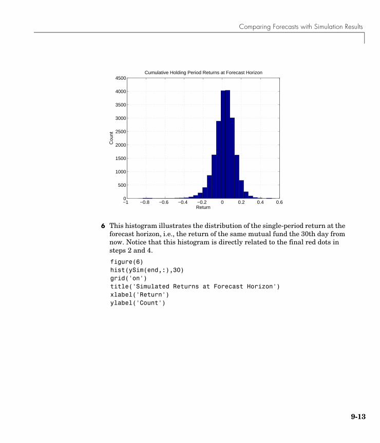
Comparing Forecasts with Simulation Results
9-13
6 This histogram illustrates the distribution of the single-period return at the forecast horizon, i.e., the return of the same mutual fund the 30th day from now. Notice that this histogram is directly related to the final red dots in steps 2 and 4.
figure(6)hist(ySim(end,:),30)grid('on')title('Simulated Returns at Forecast Horizon')xlabel('Return')ylabel('Count')
−1 −0.8 −0.6 −0.4 −0.2 0 0.2 0.4 0.60
500
1000
1500
2000
2500
3000
3500
4000
4500Cumulative Holding Period Returns at Forecast Horizon
Return
Cou
nt

9 Advanced Example
9-14
Note This example is not meant to imply that such elaborate conditional mean and variance models are required to describe typical financial time series, nor is it meant to imply that most users will need to perform such detailed analyses at all. Furthermore, it is not meant to imply that such a graphical analysis even makes sense for a given model, or that this is the only graphs that could make sense.
This example merely highlights the range of possibilities, and provides a deeper understanding of the interaction between the simulation, forecasting, and estimation engines, garchsim, garchpred, and garchfit, respectively.
−0.15 −0.1 −0.05 0 0.05 0.1 0.15 0.20
1000
2000
3000
4000
5000
6000
7000Simulated Returns at Forecast Horizon
Return
Cou
nt

10
Function Reference

10 Function Reference
10-2
Functions – By CategoryThis section lists the GARCH Toolbox functions according to their purpose.
• “GARCH Modeling” on page 10-2
• “GARCH Innovations Inference” on page 10-2
• “Statistics and Tests” on page 10-2
• “GARCH Specification Structure Interface Functions” on page 10-3
• “Helpers and Utilities” on page 10-3
• “Graphics” on page 10-3
GARCH Modeling
GARCH Innovations Inference
Statistics and Tests
garchfit Univariate GARCH process parameter estimation.
garchpred Univariate GARCH process forecasting.
garchsim Univariate GARCH process simulation.
garchinfer Inverse filter to infer GARCH innovations and conditional standard deviations from an observed return series.
aicbic Akaike and Bayesian information criteria for model order selection.
archtest Engle’s hypothesis test for the presence of ARCH/GARCH effects.
autocorr Plot or return computed sample autocorrelation function.
crosscorr Plot or return computed sample crosscorrelation function.
lbqtest Ljung-Box Q-statistic lack-of-fit hypothesis test.

Functions – By Category
10-3
GARCH Specification Structure Interface Functions
Helpers and Utilities
Graphics
lratiotest Likelihood ratio hypothesis test.
parcorr Plot or return computed sample partial autocorrelation function.
garchget Retrieve a GARCH specification structure parameter.
garchset Create or modify a GARCH specification structure.
garchar Convert finite-order ARMA models to infinite-order AR models.
garchcount Count GARCH estimation coefficients.
garchdisp Display GARCH process estimation results.
garchma Convert finite-order ARMA models to infinite-order MA models.
lagmatrix Create a lagged time-series matrix.
price2ret Convert price series to a return series.
ret2price Convert return series to a price series.
garchplot Plot matched univariate innovations, volatility, and return series.

10 Function Reference
10-4

aicbic
10-7
10aicbicPurpose Akaike (AIC) and Bayesian (BIC) information criteria for model order selection
Syntax AIC = aicbic(LLF,NumParams)[AIC,BIC] = aicbic(LLF,NumParams,NumObs)
Description aicbic computes the Akaike and Bayesian information criteria, using optimized log-likelihood objective function (LLF) values as input. You can obtain the LLF values by fitting models of the conditional mean and variance to a univariate return series.
AIC = aicbic(LLF,NumParams) computes only the Akaike (AIC) information criteria.
[AIC,BIC] = aicbic(LLF,NumParams,NumObs) computes both the Akaike (AIC) and Bayesian (BIC) information criteria.
Since information criteria penalize models with additional parameters, parsimony is the basis of the AIC and BIC model order selection criteria.
Input Arguments
LLF Vector of optimized log-likelihood objective function (LLF) values associated with parameter estimates of the models to be tested. aicbic assumes you obtained the LLF values from the estimation function garchfit or the inference function garchinfer.
NumParams Number of estimated parameters associated with each LLF value in LLF. NumParams can be a scalar applied to all values in LLF, or a vector the same length as LLF. All elements of NumParams must be positive integers. Use garchcount to compute NumParams values.
NumObs Sample size of the observed return series you associate with each value of LLF. NumObs can be a scalar applied to all values in LLF, or a vector the same length as LLF. It is required to compute BIC. All elements of NumObs must be positive integers.

aicbic
10-8
Output Arguments
Examples See “Akaike and Bayesian Information Criteria” on page 8-5.
See Also garchdisp, garchfit, garchinfer
References [1] Box, G.E.P., G.M. Jenkins, and G.C. Reinsel, Time Series Analysis: Forecasting and Control, Third edition, Prentice Hall, 1994.
AIC Vector of AIC statistics associated with each LLF objective function value. The AIC statistic is defined as
BIC Vector of BIC statistics associated with each LLF objective function value. The BIC statistic is defined as
AIC 2– LLF×( ) 2 NumParams×( )+=
BIC 2– LLF×( )NumParams log NumObs( )×( )+
=

archtest
10-9
10archtestPurpose Engle’s hypothesis test for the presence of ARCH/GARCH effects
Syntax [H,pValue,ARCHstat,CriticalValue] = archtest(Residuals,Lags,Alpha)
Description [H,pValue,ARCHstat,CriticalValue] = archtest(Residuals,Lags,Alpha)tests the null hypothesis that a time series of sample residuals consists of independent identically distributed (i.i.d.) Gaussian disturbances, i.e., that no ARCH effects exist.
Given sample residuals obtained from a curve fit (e.g., a regression model), archtest tests for the presence of th order ARCH effects by regressing the squared residuals on a constant and the lagged values of the previous squared residuals. Under the null hypothesis, the asymptotic test statistic,
, where is the number of squared residuals included in the regression and is the sample multiple correlation coefficient, is asymptotically chi-square distributed with degrees of freedom. When testing for ARCH effects, a GARCH(P,Q) process is locally equivalent to an ARCH(P+Q) process.
Input Arguments
Output Arguments
MM
T R2( ) T
R2
M
Residuals Time-series column vector of sample residuals obtained from a curve fit, which archtest examines for the presence of ARCH effects. The last row contains the most recent observation.
Lags Vector of positive integers indicating the lags of the squared sample residuals included in the ARCH test statistic. If specified, each lag should be significantly less than the length of Residuals. If Lags = [] or is not specified, the default is 1 lag (i.e., first-order ARCH).
Alpha Significance levels of the hypothesis test. Alpha can be a scalar applied to all lags in Lags, or a vector of significance levels the same length as Lags. If Alpha = [] or is not specified, the default is 0.05. For all elements, , of Alpha,
.α
0 α 1< <
H Boolean decision vector. 0 indicates acceptance of the null hypothesis that no ARCH effects exist; i.e., there is homoscedasticity at the corresponding element of Lags. 1 indicates rejection of the null hypothesis. The length of H is the same as the length of Lags.

archtest
10-10
Examples Example 1. Create a time-series column vector of 100 (synthetic) residuals, then test for the first, second, and fourth order ARCH effects at the 10 percent significance level.
randn('state',0) % Start from a known state.residuals = randn(100,1); % 100 Gaussian deviates ~ N(0,1)[H,P,Stat,CV] = archtest(residuals,[1 2 4]',0.10);[H,P,Stat,CV]
ans =
0 0.3925 0.7312 2.7055 0 0.5061 1.3621 4.6052 0 0.7895 1.7065 7.7794
Example 2. See “Analysis and Estimation Example Using the Default Model” on page 2-15 for another example.
See Also lbqtest
References [1] Box, G.E.P., G.M. Jenkins, and G.C. Reinsel, Time Series Analysis: Forecasting and Control, Third edition, Prentice Hall, 1994.
[2] Engle, Robert, “Autoregressive Conditional Heteroskedasticity with Estimates of the Variance of United Kingdom Inflation,” Econometrica, Vol. 50, 1982, pp 987-1007.
[3] Gourieroux, C., ARCH Models and Financial Applications, Springer-Verlag, 1997.
[4] Hamilton, J.D., Time Series Analysis, Princeton University Press, 1994.
pValue Vector of P-values (significance levels) at which archtest rejects the null hypothesis of no ARCH effects at each lag in Lags.
ARCHstat Vector of ARCH test statistics for each lag in Lags.
CriticalValue Vector of critical values of the chi-square distribution for comparison with the corresponding element of ARCHstat.

autocorr
10-11
10autocorrPurpose Plot or return computed sample autocorrelation function
Syntax autocorr(Series,nLags,M,nSTDs)[ACF,Lags,Bounds] = autocorr(Series,nLags,M,nSTDs)
Description autocorr(Series,nLags,M,nSTDs) computes and plots the sample ACF of a univariate, stochastic time series with confidence bounds. To plot the ACF sequence without the confidence bounds, set nSTDs = 0.
[ACF,Lags,Bounds] = autocorr(Series,nLags,M,nSTDs) computes and returns the ACF sequence.
Input Arguments
Series Column vector of observations of a univariate time series for which autocorr computes or plots the sample autocorrelation function (ACF). The last row of Series contains the most recent observation of the time series.
nLags Positive scalar integer indicating the number of lags of the ACF to compute. If nLags = [] or is not specified, the default is to compute the ACF at lags 0, 1, 2, ..., , where
= min([20,length(Series)-1]).
M Nonnegative integer scalar indicating the number of lags beyond which the theoretical ACF is effectively 0. autocorr assumes the underlying Series is an MA(M) process, and uses Bartlett’s approximation to compute the large-lag standard error for lags greater than M. If M = [] or is not specified, the default is 0, and autocorr assumes that Series is Gaussian white noise. If Series is a Gaussian white noise process of length , the standard error is approximately . M must be less than nLags.
nSTDs Positive scalar indicating the number of standard deviations of the sample ACF estimation error to compute. autocorr assumes the theoretical ACF of Series is 0 beyond lag M. When M = 0 and Series is a Gaussian white noise process of length , specifying nSTDs results in confidence bounds at . If nSTDs = [] or is not specified, the default is 2 (i.e., approximate 95 percent confidence interval).
TT
N1 N⁄
NnSTDs N⁄( )±

autocorr
10-12
Output Arguments
Examples Example 1. Create an MA(2) time series from a column vector of 1000 Gaussian deviates, and assess whether the ACF is effectively zero for lags greater than 2.
randn('state',0) % Start from a known state.x = randn(1000,1); % 1000 Gaussian deviates ~ N(0,1).y = filter([1 -1 1],1,x); % Create an MA(2) process.[ACF,Lags,Bounds] = autocorr(y,[],2); % Compute the ACF with % 95 percent confidence.[Lags, ACF]
ans = 0 1.0000 1.0000 -0.6487 2.0000 0.3001 3.0000 0.0229 4.0000 0.0196 5.0000 -0.0489 6.0000 0.0452 7.0000 0.0012 8.0000 -0.0214 9.0000 0.0235 10.0000 0.0340 11.0000 -0.0392 12.0000 0.0188 13.0000 0.0504 14.0000 -0.0600
ACF Sample autocorrelation function of Series. ACF is a vector of length nLags+1 corresponding to lags 0, 1, 2, ..., nLags. The first element of ACF is unity, that is, ACF(1) = 1 = lag 0 correlation.
Lags Vector of lags corresponding to ACF(0,1,2,...,nLags). Since an ACF is symmetric about 0 lag, autocorr ignores negative lags.
Bounds Two-element vector indicating the approximate upper and lower confidence bounds, assuming that Series is an MA(M) process. Values of ACF beyond lag M that are effectively 0 lie within these bounds. Note that autocorr computes Bounds only for lags greater than M.

autocorr
10-13
15.0000 0.0251 16.0000 0.0441 17.0000 -0.0732 18.0000 0.0755 19.0000 -0.0571 20.0000 0.0485
Bounds
Bounds = 0.0899 -0.0899
autocorr(y,[],2) % Use the same example, but plot the ACF % sequence with confidence bounds.
Example 2. See “Analysis and Estimation Example Using the Default Model” on page 2-15 for another example.
0 5 10 15 20−0.8
−0.6
−0.4
−0.2
0
0.2
0.4
0.6
0.8
1
Lag
Sam
ple
Aut
ocor
rela
tion
Sample Autocorrelation Function (ACF)

autocorr
10-14
See Also crosscorr, parcorrfilter (MATLAB)
References [1] Box, G.E.P., G.M. Jenkins, and G.C. Reinsel, Time Series Analysis: Forecasting and Control, Third edition, Prentice Hall, 1994.
[2] Hamilton, J.D., Time Series Analysis, Princeton University Press, 1994.

crosscorr
10-15
10crosscorrPurpose Plot or return computed sample crosscorrelation function
Syntax crosscorr(Series1,Series2,nLags,nSTDs)[XCF,Lags,Bounds] = crosscorr(Series1,Series2,nLags,nSTDs)
Description crosscorr(Series1,Series2,nLags,nSTDs) computes and plots the sample crosscorrelation function (XCF) between two univariate, stochastic time series. To plot the XCF sequence without the confidence bounds, set nSTDs = 0.
[XCF,Lags,Bounds] = crosscorr(Series1,Series2,nLags,nSTDs)computes and returns the XCF sequence.
Input Arguments
Output Arguments
Series1 Column vector of observations of the first univariate time series for which crosscorr computes or plots the sample crosscorrelation function (XCF). The last row of Series1 contains the most recent observation.
Series2 Column vector of observations of the second univariate time series for which crosscorr computes or plots the sample XCF. The last row of Series2 contains the most recent observation.
nLags Positive scalar integer indicating the number of lags of the XCF to compute. If nLags = [] or is not specified, crosscorr computes the XCF at lags , where
= min([20,min([length(Series1),length(Series2)])-1]).
nSTDs Positive scalar indicating the number of standard deviations of the sample XCF estimation error to compute, if Series1 and Series2 are uncorrelated. If nSTDs = [] or is not specified, the default is 2 (i.e., approximate 95 percent confidence interval).
0 1± 2± … T±, , , ,T
XCF Sample crosscorrelation function between Series1 and Series2. XCF is a vector of length 2(nLags)+1, which corresponds to lags
. The center element of XCF contains the 0th lag cross correlation.
Lags Vector of lags corresponding to XCF(-nLags, ..., +nLags).
0 1± 2± … nLAGs±, , , ,

crosscorr
10-16
Examples Example 1. Create a time-series column vector of 100 Gaussian deviates, and a delayed version lagged by four samples. Compute the XCF, and then plot it to see the XCF peak at the fourth lag.
randn('state',100) % Start from a known state.x = randn(100,1); % 100 Gaussian deviates, N(0,1).y = lagmatrix(x,4); % Delay it by 4 samples.y(isnan(y)) = 0; % Replace NaNs with zeros.[XCF,Lags,Bounds] = crosscorr(x,y); % Compute the XCF with % 95 percent confidence.[Lags, XCF]
ans =
-20.0000 -0.0210 -19.0000 -0.0041 -18.0000 0.0661 -17.0000 0.0668 -16.0000 0.0380 -15.0000 -0.1060 -14.0000 0.0235 -13.0000 0.0240 -12.0000 0.0366 -11.0000 0.0505 -10.0000 0.0661 -9.0000 0.1072 -8.0000 -0.0893 -7.0000 -0.0018 -6.0000 0.0730 -5.0000 0.0204 -4.0000 0.0352 -3.0000 0.0792 -2.0000 0.0550 -1.0000 0.0004 0 -0.1556
Bounds Two-element vector indicating the approximate upper and lower confidence bounds, assuming that Series1 and Series2 are completely uncorrelated.
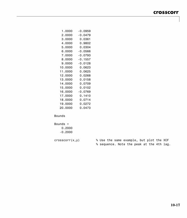
crosscorr
10-17
1.0000 -0.0959 2.0000 -0.0479 3.0000 0.0361 4.0000 0.9802 5.0000 0.0304 6.0000 -0.0566 7.0000 -0.0793 8.0000 -0.1557 9.0000 -0.0128 10.0000 0.0623 11.0000 0.0625 12.0000 0.0268 13.0000 0.0158 14.0000 0.0709 15.0000 0.0102 16.0000 -0.0769 17.0000 0.1410 18.0000 0.0714 19.0000 0.0272 20.0000 0.0473
Bounds
Bounds = 0.2000 -0.2000
crosscorr(x,y) % Use the same example, but plot the XCF % sequence. Note the peak at the 4th lag.

crosscorr
10-18
Example 2. See “Analysis and Estimation Example Using the Default Model” on page 2-15 for another example.
See Also autocorr, parcorrfilter (MATLAB)
−20 −15 −10 −5 0 5 10 15 20−0.2
0
0.2
0.4
0.6
0.8
1
1.2
Lag
Sam
ple
Cro
ss C
orre
latio
n
Sample Cross Correlation Function (XCF)

garchar
10-19
10garcharPurpose Convert finite-order ARMA models to infinite-order autoregressive (AR) models
Syntax InfiniteAR = garchar(AR,MA,NumLags)
Description InfiniteAR = garchar(AR,MA,NumLags) computes the coefficients of an infinite-order AR model, using the coefficients of the equivalent univariate, stationary, invertible, finite-order ARMA(R,M) model as input. garchar truncates the infinite-order AR coefficients to accommodate a user-specified number of lagged AR coefficients.
Input Arguments
Output Arguments
In the following ARMA(R,M) model, is the return series of interest and the innovations noise process.
AR R-element vector of autoregressive coefficients associated with the lagged observations of a univariate return series modeled as a finite-order, stationary, invertible ARMA(R,M) model.
MA M-element vector of moving-average coefficients associated with the lagged innovations of a finite-order, stationary, invertible univariate ARMA(R,M) model.
NumLags (optional) Number of lagged AR coefficients that garchar includes in the approximation of the infinite-order AR representation. NumLags is an integer scalar and determines the length of the infinite-order AR output vector. If NumLags = [] or is not specified, the default is 10.
InfiniteAR Vector of coefficients of the infinite-order AR representation associated with the finite-order ARMA model specified by the AR and MA input vectors. InfiniteAR is a vector of length NumLags. The jth element of InfiniteAR is the coefficient of the jth lag of the input series in an infinite-order AR representation. Note that Box, Jenkins, and Reinsel refer to the infinite-order AR coefficients as “ weights.”π
yt{ }εt{ }

garchar
10-20
If you write this model equation as
you can specify the garchar input coefficient vectors, AR and MA, exactly as you read them from the model. In general, the jth elements of AR and MA are the coefficients of the jth lag of the return series and innovations processes and , respectively. garchar assumes that the current-time-index coefficients of and are 1 and are not part of AR and MA.
In theory, you can use the weights returned in InfiniteAR to approximate as a pure AR process.
Consistently, the jth element of the truncated infinite-order autoregressive output vector, or InfiniteAR(j), is the coefficient of the jth lag of the observed return series, , in this equation. See Box, Jenkins, and Reinsel [8], Section 4.2.3, pages 106-109.
Examples For the following ARMA(2,2) model, use garchar to obtain the first 20 weights of the infinite-order AR approximation.
From this model,
AR = [0.5 -0.8] MA = [-0.6 0.08]
Since the current-time-index coefficients of and are defined to be 1, the example omits them from AR and MA. This saves time and effort when you specify parameters using the garchset and garchget interfaces.
PI = garchar([0.5 -0.8], [-0.6 0.08], 20);PI'
yt φiyt i–i 1=
R
∑ εt θjεt j–
j 1=
M
∑+ +=
yt φ1yt 1– … φRyt R– εt θ1εt 1– … θMεt M–+ + + + + +=
yt j–εt j–
yt εt
πyt
yt πiyt i–i 1=
∞
∑ εt+=
πjyt j–
yt 0.5yt 1– 0.8yt 2–– εt 0.6εt 1– 0.08εt 2–+–+=
yt εt
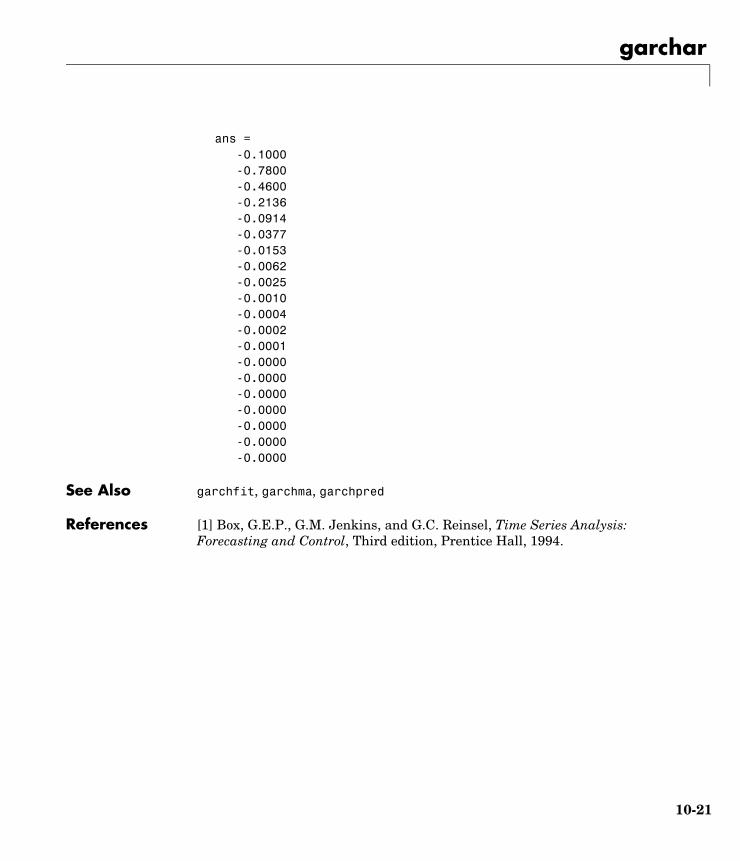
garchar
10-21
ans = -0.1000 -0.7800 -0.4600 -0.2136 -0.0914 -0.0377 -0.0153 -0.0062 -0.0025 -0.0010 -0.0004 -0.0002 -0.0001 -0.0000 -0.0000 -0.0000 -0.0000 -0.0000 -0.0000 -0.0000
See Also garchfit, garchma, garchpred
References [1] Box, G.E.P., G.M. Jenkins, and G.C. Reinsel, Time Series Analysis: Forecasting and Control, Third edition, Prentice Hall, 1994.

garchcount
10-22
10garchcountPurpose Count number of GARCH estimation coefficients
Syntax NumParams = garchcount(Coeff)
Description NumParams = garchcount(Coeff) counts and returns the number of estimated coefficients from a specification structure, as returned by garchfit, containing coefficient estimates and equality constraint information. garchcount is a helper utility designed to support the model selection function aicbic.
Input Arguments
Output Arguments
Example See “Akaike and Bayesian Information Criteria” on page 8-5.
See Also aicbic, garchdisp, garchfit
Coeff Specification structure containing coefficient estimates and equality constraints. Coeff is an output of the estimation function garchfit.
NumParams Number of estimated parameters, i.e., coefficients, included in the conditional mean and variance specifications, less any parameters held constant, as equality constraints, during the estimation. The aicbic function needs NumParams to calculate the Akaike (AIC) and Bayesian (BIC) statistics.

garchdisp
10-23
10garchdispPurpose Display estimation results
Syntax garchdisp(Coeff,Errors)
Description garchdisp(Coeff,Errors) displays coefficient estimates, standard errors, and T-statistics from a GARCH specification structure that was output by the estimation function garchfit.
This function displays estimation results, and returns no output arguments. The tabular display includes parameter estimates, standard errors, and T-statistics for each parameter in the conditional mean and variance models. Parameters held fixed during the estimation process have the word 'Fixed' displayed in the standard error and T-statistic columns, indicating that the parameter was set as an equality constraint.
Input Arguments
Examples The following code uses garchfit to generate the GARCH specification structure Coeff and the standard errors structure Errors for a return series of 1000 simulated observations based on a GARCH(1,1) model. It then calls garchdisp to display the estimation results. Setting 'Display' to 'off' suppresses display of the iterative optimization information produced by garchfit.
spec = garchset('C',0,'K',0.0001,'GARCH',0.9,'ARCH',0.05,... 'Display','off');[e,s,y] = garchsim(spec,1000);[Coeff,Errors] = garchfit(spec,y);garchdisp(Coeff,Errors)
Mean: ARMAX(0,0,0); Variance: GARCH(1,1) Conditional Probability Distribution: Gaussian Number of Model Parameters Estimated: 4
Coeff GARCH specification structure containing estimated coefficients and equality constraint information. Coeff is an output of the estimation function garchfit.
Errors Structure containing the estimation errors (i.e., the standard errors) of the coefficients in Coeff. Errors is also an output of the estimation function garchfit.

garchdisp
10-24
Standard T Parameter Value Error Statistic ----------- ----------- ------------ ----------- C -0.0024759 0.0012919 -1.9165 K 4.6877e-005 5.3555e-005 0.8753 GARCH(1) 0.93904 0.041604 22.5707 ARCH(1) 0.035503 0.015123 2.3477
See Also garchcount, garchfit

garchfit
10-25
10garchfitPurpose Univariate GARCH process parameter estimation
Syntax [Coeff,Errors,LLF,Innovations,Sigmas,Summary] = garchfit(Series)[...] = garchfit(Spec,Series)[...] = garchfit(Spec,Series,X)[...] = garchfit(Spec,Series,X,PreInnovations,PreSigmas,PreSeries)garchfit(...)
Description Given an observed univariate return series, garchfit estimates the parameters of a conditional mean specification of ARMAX form, and conditional variance specification of GARCH, EGARCH, or GJR form. The estimation process infers the innovations (i.e., residuals) from the return series, and fits the model specification to the return series by maximum likelihood.
[Coeff,Errors,LLF,Innovations,Sigmas,Summary] = garchfit(Series)models an observed univariate return series as a constant, C, plus GARCH(1,1) conditionally Gaussian innovations. For models beyond this simple (yet common) model, you must provide model parameters in the GARCH specification structure Spec.
[...] = garchfit(Spec,Series) infers the innovations from the return series and fits the model specification, contained in Spec, to the return series by maximum likelihood.
[...] = garchfit(Spec,Series,X) provides a regression component X for the conditional mean.
[...] = garchfit(Spec,Series,X,PreInnovations,PreSigmas,PreSeries)uses presample observations, contained in the time-series column vectors PreInnovations, PreSigmas, and PreSeries, to infer the outputs Innovations and Sigmas. These vectors form the conditioning set used to initiate the inverse filtering, or inference, process. If you provide no explicit presample data, the necessary presample observations are derived by conventional time-series techniques (see “Automatic Minimization of Transient Effects” on page 4-6).
If you specify at least one set, but fewer than three sets, of presample data, garchsim does not attempt to derive presample observations for those you omit. If you specify your own presample data, you must specify all that are necessary
garchfit
10-26
for the specified conditional mean and variance models. See “User-Specified Presample Observations” on page 5-11.
garchfit(...) (with input arguments as shown above but with no output arguments) displays the final parameter estimates and standard errors. It also produces a tiered plot of the original return series, the inferred innovations, and the corresponding conditional standard deviations.
Input Arguments
Spec GARCH specification structure containing the conditional mean and variance specifications. It also contains the optimization parameters needed for the estimation.Create this structure by calling garchset, or use the Coeff output structure returned by garchfit.
Series Time-series column vector of observations of the underlying univariate return series of interest. Series is the response variable representing the time series to be fitted to conditional mean and variance specifications. The last element of Series holds the most recent observation.
X Time-series regression matrix of observed explanatory data. Typically, X is a matrix of asset returns (e.g., the return series of an equity index), and represents the past history of the explanatory data. Each column of X is an individual time series used as an explanatory variable in the regression component of the conditional mean. In each column, the first row contains the oldest observation and the last row the most recent.
The number of valid (non-NaN) most recent observations in each column of X must equal or exceed the number of valid most recent observations in Series. If the number of valid observations in a column of X exceeds that of Series, garchfit uses only the most recent observations of X. If X = [] or is not specified, the conditional mean has no regression component.

garchfit
10-27
PreInnovations Time-series column vector of presample innovations that garchfit uses to condition the recursive mean and variance models. This column vector can have any number of rows, provided it contains sufficient observations to initialize the mean and variance equations. I.e., if M and Q are the number of lagged innovations required by the conditional mean and variance equations, respectively, then PreInnovations must have at least max(M,Q) rows. If the number of rows exceeds max(M,Q), then garchfit uses only the last (i.e., most recent) max(M,Q) rows.
PreSigmas Time-series column vector of positive presample conditional standard deviations that garchfit uses to condition the recursive variance model. This vector can have any number of rows, provided it contains sufficient observations to initialize the conditional variance equation. I.e., if P and Q are the number of lagged conditional standard deviations and lagged innovations required by the conditional variance equation, respectively, then PreSigmas must have at least P rows for GARCH and GJR models, and at least max(P,Q) rows for EGARCH models. If the number of rows exceeds the requirement, then garchfit uses only the last (i.e., most recent) rows.
PreSeries Time-series column vector of presample observations of the return series of interest that garchfit uses to condition the recursive mean model. This vector can have any number of rows, provided it contains sufficient observations to initialize the conditional mean equation. Thus, if R is the number of lagged observations of the return series required by the conditional mean equation, then PreSeries must have at least R rows. If the number of rows exceeds R, then garchfit uses only the last (i.e., most recent) R rows.

garchfit
10-28
Output Arguments
Coeff GARCH specification structure containing the estimated coefficients. Coeff is of the same form as the Spec input structure. Toolbox functions such as garchset, garchget, garchsim, garchinfer, and garchpred can accept either Spec or Coeff as input arguments.
Errors Structure containing the estimation errors (i.e., the standard errors) of the coefficients. Errors is of the same form as the Spec and Coeff structures.
LLF Optimized log-likelihood objective function value associated with the parameter estimates found in Coeff. garchfit performs the optimization using the fmincon function of the Optimization Toolbox.
Innovations Innovations (i.e., residuals) time-series column vector inferred from Series. The size of Innovations is the same as the size of Series.
Sigmas Conditional standard deviation vector corresponding to Innovations. The size of Sigmas is the same as the size of Series.
Summary Structure of summary information about the optimization process. The fields and their possible values are
warning One of the following strings:
'No Warnings''ARMA Model Is Not Stationary/Invertible'
converge One of the following strings:
'Function Converged to a Solution''Function Did NOT Converge''Maximum Function Evaluations or Iterations Reached'
constraints One of the following strings:
'No Boundary Constraints''Boundary Constraints Active; Errors May Be Inaccurate'

garchfit
10-29
Note garchfit calculates the error covariance matrix of the parameter estimates Summary.covMatrix, and the corresponding standard errors found in the Errors output structure using finite difference approximation. In particular, it calculates the standard errors using the outer-product method (see Hamilton [8], Section 5.8, bottom of page 143).
Example 1 The following code uses garchfit to estimate the parameters for a return series of 1000 simulated observations based on a GARCH(1,1) model. Because the 'Display' parameter defaults to 'on', garchfit displays diagnostic and iterative information.
spec = garchset('C',0,'K',0.0001,'GARCH',0.9,'ARCH',0.05);[e,s,y] = garchsim(spec,1000);[Coeff,Errors] = garchfit(spec,y);
%%%%%%%%%%%%%%%%%%%%%%%%%%%%%%%%%%%%%%%%%%%%%%%%%%%%%%%%%%% Diagnostic Information
Number of variables: 4
Functions Objective: garchllfn Gradient: finite-differencing Hessian: finite-differencing (or Quasi-Newton) Nonlinear constraints: armanlc Gradient of nonlinear constraints: finite-differencing
Constraints Number of nonlinear inequality constraints: 0 Number of nonlinear equality constraints: 0
covMatrix Covariance matrix of the parameter estimates
iterations Number of iterations
functionCalls Number of function evaluations
lambda Structure, output by fmincon, containing the Lagrange multipliers at the solution x

garchfit
10-30
Number of linear inequality constraints: 1 Number of linear equality constraints: 0 Number of lower bound constraints: 4 Number of upper bound constraints: 4
Algorithm selected medium-scale
%%%%%%%%%%%%%%%%%%%%%%%%%%%%%%%%%%%%%%%%%%%%%%%%%%%%%%%%%%% End diagnostic information
max Directional First-order Iter F-count f(x) constraint Step-size derivative optimality Procedure 1 22 -1762.62 -9.975e-005 0.000488 1.32e+004 1.47e+004 2 35 -1763.04 -9.897e-005 0.00781 126 2.13e+005 3 43 -1764.69 -7.423e-005 0.25 4.19 1.28e+005 4 57 -1764.72 -7.477e-005 0.00391 6.92 1.12e+005 5 64 -1765.27 -4.128e-005 0.5 0.228 3.59e+003 6 78 -1765.28 -4.751e-005 0.00391 3.34 2.98e+004 7 89 -1765.28 -4.617e-005 0.0313 0.0725 2.91e+004 8 101 -1765.29 -4.927e-005 0.0156 0.39 84 9 107 -1765.29 -4.73e-005 1 -0.000969 6.06 10 114 -1765.29 -4.668e-005 0.5 -0.000135 213 11 134 -1765.29 -4.668e-005 -6.1e-005 -2.4e-005 213 Hessian modified 12 140 -1765.29 -4.668e-005 1 1.39e-007 19.5 Hessian modified twice Optimization terminated successfully: Magnitude of directional derivative in search direction less than 2*options.TolFun and maximum constraint violation is less than options.TolCon No Active Constraints
Example 2 Using the same data as above, the example sets 'Display' to 'off' and calls garchfit with no output arguments. In this case, garchfit displays the final parameter estimates and standard errors, then produces a tiered plot.
spec = garchset(spec,'Display','off');garchfit(spec,y)
Mean: ARMAX(0,0,0); Variance: GARCH(1,1)
Conditional Probability Distribution: Gaussian Number of Model Parameters Estimated: 4

garchfit
10-31
Standard T Parameter Value Error Statistic ----------- ----------- ------------ ----------- C -0.0024759 0.0012919 -1.9165 K 4.6877e-005 5.3555e-005 0.8753 GARCH(1) 0.93904 0.041604 22.5707 ARCH(1) 0.035503 0.015123 2.3477
Log Likelihood Value: 1765.29
See Also garchpred, garchset, garchsim
fmincon (in the Optimization Toolbox)
References [1] Bollerslev, T., “A Conditionally Heteroskedastic Time Series Model for Speculative Prices and Rates of Return,” Review of Economics and Statistics, Vol. 69, 1987, pp 542-547.
0 200 400 600 800 1000−0.2
0
0.2Innovations
Inno
vatio
n
0 200 400 600 800 10000.02
0.04
0.06
0.08Conditional Standard Deviations
Sta
ndar
d D
evia
tion
0 200 400 600 800 1000−0.2
0
0.2Returns
Ret
urn

garchfit
10-32
[2] Bollerslev, T., “Generalized Autoregressive Conditional Heteroskedasticity,” Journal of Econometrics, Vol. 31, 1986, pp 307-327.
[3] Box, G.E.P., G.M. Jenkins, and G.C. Reinsel, Time Series Analysis: Forecasting and Control, Third edition, Prentice Hall, 1994.
[4] Enders, W., Applied Econometric Time Series, John Wiley & Sons, 1995.
[5] Engle, Robert, “Autoregressive Conditional Heteroskedasticity with Estimates of the Variance of United Kingdom Inflation,” Econometrica, Vol. 50, 1982, pp 987-1007.
[6] Engle, R.F., D.M. Lilien, and R.P. Robins, “Estimating Time Varying Risk Premia in the Term Structure: The ARCH-M Model,” Econometrica, Vol. 59, 1987, pp 391-407.
[7] Glosten, L.R., R. Jagannathan, and D.E. Runkle, “On the Relation Between Expected Value and the Volatility of the Nominal Excess Return on Stocks,” The Journal of Finance, Vol.48, 1993, pp 1779-1801.
[8] Hamilton, J.D., Time Series Analysis, Princeton University Press, 1994.
[9] Nelson, D.B., “Conditional Heteroskedasticity in Asset Returns: A New Approach,” Econometrica, Vol. 59, 1991, pp 347-370.

garchget
10-33
10garchgetPurpose Retrieve a GARCH specification structure parameter
Syntax ParameterValue = garchget(Spec,'ParameterName')
Description ParameterValue = garchget(Spec,'ParameterName') returns the value of the specified parameter from the GARCH specification structure Spec.
Input Arguments
Output Arguments
Examples Spec = garchset('P',1,'Q',1) % Create a GARCH(P=1,Q=1) model.Spec = Comment: 'Mean: ARMAX(0,0,?); Variance: GARCH(1,1)' Distribution: 'Gaussian' C: [] VarianceModel: 'GARCH' P: 1 Q: 1 K: [] GARCH: [] ARCH: []
P = garchget(Spec,'P') % Retrieve the order P.P = 1
See Also garchfit, garchpred, garchset, garchsim
Spec GARCH specification structure returned by garchset, or the output (Coeff) of the estimation function garchfit.
ParameterName String indicating the name of the parameter whose value garchget extracts from Spec. It is sufficient to type only the leading characters that uniquely identify a parameter name. See garchset for a list of valid parameter names. ParameterName is case insensitive.
ParameterValue Value of the named parameter extracted from the structure Spec. garchget returns the appropriate model default value if the specified parameter is not defined in the specification structure.

garchinfer
10-34
10garchinferPurpose Infer GARCH innovation processes from return series
Syntax [Innovations,Sigmas,LLF] = garchinfer(Spec,Series)[...] = garchinfer(Spec,Series,X)[...] = garchinfer(Spec,Series,X,... PreInnovations,PreSigmas,PreSeries)
Description [Innovations,Sigmas,LLF] = garchinfer(Spec,Series) given a conditional mean specification of ARMAX form and conditional variance specification of GARCH, EGARCH, or GJR form, infers the innovations and conditional standard deviations from an observed univariate return series. Since garchinfer is an interface to the appropriate log-likelihood objective function, the log-likelihood value is also computed for convenience.
[...] = garchinfer(Spec,Series,X) also accepts a time-series regression matrix X of observed explanatory data. garchinfer treats each column of X as an individual time series, and uses it as an explanatory variable in the regression component of the conditional mean.
[...] = garchinfer(Spec,Series,X,PreInnovations,PreSigmas, PreSeries) uses presample observations, contained in the time-series matrices or column vectors PreInnovations, PreSigmas, and PreSeries, to infer the outputs Innovations and Sigmas. These vectors form the conditioning set used to initiate the inverse filtering, or inference, process.
If you specify the presample data as matrices, the number of columns (realizations) of each must be the same as the number of columns (realizations) of the Series input. In this case, the presample information of a given column is used to infer the residuals and standard deviations of the corresponding column of Series. If you specify the presample data as column vectors, the vectors are applied to each column of Series.
If you provide no explicit presample data, the necessary presample observations are derived by conventional time-series techniques (see “Automatic Minimization of Transient Effects” on page 4-6.
If you specify at least one set, but fewer than three sets, of presample data, garchsim does not attempt to derive presample observations for those you omit. If you specify your own presample data, you must specify all that are necessary

garchinfer
10-35
for the specified conditional mean and variance models. See “User-Specified Presample Observations” on page 5-11.
Input Arguments
Spec GARCH specification structure containing the conditional mean and variance specifications. It also contains the optimization parameters needed for the estimation.Create this structure by calling garchset, or use the Coeff output structure returned by garchfit.
Series Time-series matrix or column vector of observations of the underlying univariate return series of interest. Series is the response variable representing the time series fitted to conditional mean and variance specifications. Each column of Series in an independent realization (i.e., path). The last row of Series holds the most recent observation of each realization.
X Time-series regression matrix of explanatory variables. Typically, X is a regression matrix of asset returns (e.g., the return series of an equity index). Each column of X is an individual time series used as an explanatory variable in the regression component of the conditional mean. In each column, the first row contains the oldest observation and the last row the most recent.
The number of valid (non-NaN) observations below the last NaN in each column of X must equal or exceed the number of valid observations below the last NaN in Series. If the number of valid observations in a column of X exceeds that of Series, garchinfer uses only the most recent. If X = [] or is not specified, the conditional mean has no regression component.

garchinfer
10-36
PreInnovations Time-series matrix or column vector of presample innovations on which the recursive mean and variance models are conditioned. This array can have any number of rows, provided it contains sufficient observations to initialize the mean and variance equations. I.e., if M and Q are the number of lagged innovations required by the conditional mean and variance equations, respectively, then PreInnovations must have at least max(M,Q) rows.
If the number of rows exceeds max(M,Q), then only the last (i.e., most recent) max(M,Q) rows are used. If PreInnovations is a matrix, then the number of columns must be the same as the number of columns in Series. If PreInnovations is a column vector, then the vector is applied to each column (i.e., realization) of Series.
PreSigmas Time-series matrix or column vector of positive presample conditional standard deviations on which the recursive variance model is conditioned. This array can have any number of rows, provided it contains sufficient observations to initialize the conditional variance equation. I.e., if P and Q are the number of lagged conditional standard deviations and lagged innovations required by the conditional variance equation, respectively, then PreSigmas must have at least P rows for GARCH and GJR models, and at least max(P,Q) rows for EGARCH models.
If the number of rows exceeds the requirement, then only the last (i.e., most recent) rows are used. If PreSigmas is a matrix, then the number of columns must be the same as the number of columns in Series. If PreSigmas is a column vector, then the vector is applied to each column (i.e., realization) of Series.
garchinfer
10-37
Output Arguments
Remarks garchinfer performs essentially the same operation as garchfit, but without the optimization. While garchfit calls the appropriate log-likelihood objective function indirectly via the iterative numerical optimizer, garchinfer allows you direct access to the same suite of log-likelihood objective functions.
Note that, for garchinfer, inputs Series, PreInnovations, PreSigmas, and PreSeries, and outputs Innovations and Sigmas, are column-oriented time-series arrays in which each column is associated with a unique realization, or random path. For garchfit, these same inputs and outputs cannot have multiple columns; i.e., they must all represent single realizations of a univariate time series.
PreSeries Time-series matrix or column vector of presample observations of the return series of interest on which the recursive mean model is conditioned. This array can have any number of rows, provided it contains sufficient observations to initialize the conditional mean equation. Thus, if R is the number of lagged observations of the return series required by the conditional mean equation, then PreSeries must have at least R rows. If the number of rows exceeds R, then only the last (i.e., most recent) R rows are used. If PreSeries is a matrix, then the number of columns must be the same as the number of columns in Series. If PreSeries is a column vector, then the vector is applied to each column (i.e., realization) of Series.
Innovations Innovations time-series matrix inferred from Series. The size of Innovations is the same as the size of Series.
Sigmas Conditional standard deviation time-series matrix corresponding to Innovations. The size of Sigmas is the same as the size of Series.
LLF Row vector of log-likelihood objective function values for each realization of Series. The length of LLF is the same as the number of columns in Series.

garchinfer
10-38
For additional details about estimation and inverse filtering, see “Maximum Likelihood Estimation” on page 5-2 and “Presample Observations” on page 5-11.
Examples See “Presample Data and Transient Effects” on page 5-23, “Presample Observations” on page 6-5, and “Estimating the Model” on page 9-2.
See Also garchfit, garchpred, garchset, garchsim
References [1] Box, G.E.P., G.M. Jenkins, and G.C. Reinsel, Time Series Analysis: Forecasting and Control, Third edition, Prentice Hall, 1994.
[2] Hamilton, J.D., Time Series Analysis, Princeton University Press, 1994.

garchma
10-39
10garchmaPurpose Convert finite-order ARMA models to infinite-order moving average (MA) models
Syntax InfiniteMA = garchma(AR,MA,NumLags)
Description InfiniteMA = garchma(AR,MA,NumLags) computes the coefficients of an infinite-order MA model, using the coefficients of the equivalent univariate, stationary, invertible, finite-order ARMA(R,M) model as input. garchma truncates the infinite-order MA coefficients to accommodate the number of lagged MA coefficients you specify in NumLags.
This function is particularly useful for calculating the standard errors of minimum mean square error forecasts of univariate ARMA models.
Arguments
Output Arguments
In the following ARMA(R,M) model, is the return series of interest and the innovations noise process.
AR R-element vector of autoregressive coefficients associated with the lagged observations of a univariate return series modeled as a finite-order, stationary, invertible ARMA(R,M) model.
MA M-element vector of moving-average coefficients associated with the lagged innovations of a finite-order, stationary, invertible, univariate ARMA(R,M) model.
NumLags (optional) Number of lagged MA coefficients that garchma includes in the approximation of the infinite-order MA representation. NumLags is an integer scalar and determines the length of the infinite-order MA output vector. If NumLags = [] or is not specified, the default is 10.
InfiniteMA Vector of coefficients of the infinite-order MA representation associated with the finite-order ARMA model specified by AR and MA. InfiniteMA is a vector of length NumLags. The jth element of InfiniteMA is the coefficient of the jth lag of the innovations noise sequence in an infinite-order MA representation. Note that Box, Jenkins, and Reinsel refer to the infinite-order MA coefficients as the “ weights.”ψ
yt{ }εt{ }

garchma
10-40
If you write this model equation as
you can specify the garchma input coefficient vectors, AR and MA, exactly as you read them from the model. In general, the jth elements of AR and MA are the coefficients of the jth lag of the return series and innovations processes and , respectively. garchma assumes that the current-time-index coefficients of and are 1 and are not part of AR and MA.
In theory, you can use the weights returned in InfiniteMA to approximate as a pure MA process.
Consistently, the jth element of the truncated infinite-order moving-average output vector, or InfiniteMA(j), is the coefficient of the jth lag of the innovations process, , in this equation. See Box, Jenkins, and Reinsel [8], Section 5.2.2, pages 139-141.
Examples Suppose you want a forecast horizon of 10 periods for the following ARMA(2,2) model.
To obtain probability limits for these forecasts, use garchma to compute the first 9 (i.e., 10 - 1) weights of the infinite order MA approximation.
From the model, AR = [0.5 -0.8] and MA = [-0.6 0.08].
Since the current-time-index coefficients of and are 1, the example omits them from AR and MA. This saves time and effort when you specify parameters via the garchset and garchget user interfaces.
yt φiyt i–i 1=
R
∑ εt θjεt j–
j 1=
M
∑+ +=
yt φ1yt 1– … φRyt R– εt θ1εt 1– … θMεt M–+ + + + + +=
yt j–εt j–
yt εt
ψyt
yt εt ψiεt i–
i 1=
∞
∑+=
ψjεt j–
yt 0.5yt 1– 0.8yt 2–– εt 0.6εt 1– 0.08εt 2–+–+=
yt εt

garchma
10-41
PSI = garchma([0.5 -0.8], [-0.6 0.08], 9);PSI'
ans =
-0.1000 -0.7700 -0.3050 0.4635 0.4758 -0.1329 -0.4471 -0.1172 0.2991
See Also garchar, garchpred
References [1] Box, G.E.P., G.M. Jenkins, and G.C. Reinsel, Time Series Analysis: Forecasting and Control, Third edition, Prentice Hall, 1994.

garchplot
10-42
10garchplotPurpose Plot matched univariate innovations, volatility, and return series
Syntax garchplot(Innovations,Sigmas,Series)
Description garchplot lets you visually compare matched innovations, conditional standard deviations, and returns. It provides a convenient way to compare innovations series, simulated using garchsim or estimated using garchfit, with companion conditional standard deviations, or returns series. You can also use garchplot to plot forecasts, computed using garchpred, of conditional standard deviations and returns.
In general, garchplot produces a tiered plot of matched time series. garchplot does not display an empty or missing input array; i.e., garchplot allocates no space in the tiered figure window to the array. garchplot displays valid (nonempty) Innovations, Sigmas, and Series arrays in the top, center, and bottom plots, respectively. Since garchplot assigns a title and label to each plot according to its position in the argument list, you can ensure correct plot annotation by using empty matrices ([]) as placeholders.
You can plot several realizations of each array simultaneously because garchplot color codes corresponding realizations of each input array. However, the plots can become cluttered if you try to display more than a few realizations of each input at one time.
Input Arguments
Innovations Time-series column vector or matrix of innovations. As a column vector, Innovations represents a single realization of a univariate time series in which the first element contains the oldest observation and the last element the most recent. As a matrix, each column of Innovations represents a single realization of a univariate time series in which the first row contains the oldest observation of each realization and the last row the most recent. If Innovations = [], then Innovations is not displayed.
Sigmas Time-series column vector or matrix of conditional standard deviations. In general, Innovations and Sigmas are the same size, and form a matching pair of arrays. If Sigmas = [], then Sigmas is not displayed.

garchplot
10-43
Examples Example 1. Assume that Innovations, Sigmas, and Series are not empty.
garchplot(Innovations) % Plot Innovations only.
garchplot(Innovations,[],Series) % Plot Innovations and % Series only.
garchplot([],Sigmas,Series) % Plot Sigmas and Series % only.
garchplot(Innovations,Sigmas,Series) % Plot all three vectors.
garchplot(Innovations,Sigmas,[]) % Plot Innovations and % Sigmas only.
garchplot(Innovations,Sigmas) % Plot Innovations and % Sigmas only.
Example 2. The following code uses the default GARCH(1,1) model to model the Deutschmark/British pound foreign exchange series (see “Data Sets” on page 1-11). It then uses the estimated model to generate a single path of 1000 observations for return series, innovations, and conditional standard deviation processes.
load garchdatadem2gbp = price2ret(DEM2GBP);[coeff,errors,LLF,innovations,sigmas] = garchfit(dem2gbp);[e,s,y] = garchsim(coeff,1000);garchplot(e,s,y)
Series Time-series column vector or matrix of asset returns. In general, Series is the same size as Innovations and Sigmas, and is organized in exactly the same manner. If Series = [] or is not specified, then Series is not displayed.

garchplot
10-44
See Also garchfit, garchpred, garchsim
0 200 400 600 800 1000−0.05
0
0.05Innovations
Inno
vatio
n
0 200 400 600 800 10000
0.01
0.02Conditional Standard Deviations
Sta
ndar
d D
evia
tion
0 200 400 600 800 1000−0.05
0
0.05Returns
Ret
urn

garchpred
10-45
10garchpredPurpose Univariate GARCH process forecasting
Syntax [SigmaForecast,MeanForecast] = garchpred(Spec,Series,NumPeriods)[SigmaForecast,MeanForecast] = ... garchpred(Spec,Series,NumPeriods,X,XF)[SigmaForecast,MeanForecast,SigmaTotal,MeanRMSE] = ... garchpred(Spec,Series,NumPeriods)
Description garchpred forecasts the conditional mean of the univariate return series and the standard deviation of the innovations NumPeriods into the future, using specifications for the conditional mean and variance of an observed univariate return series as input. garchpred also computes volatility forecasts of asset returns over multiperiod holding intervals, and the standard errors of conditional mean forecasts. The conditional mean is of general ARMAX form and the conditional variance can be of GARCH, EGARCH, or GJR form. (See “Conditional Mean and Variance Models” on page 2-6.)
[SigmaForecast,MeanForecast] = garchpred(Spec,Series,NumPeriods)uses the conditional mean and variance specifications defined in Spec to forecast the conditional mean, MeanForecast, of the univariate return series and the standard deviation, SigmaForecast, of the innovations NumPeriods into the future. The NumPeriods default is 1.
[SigmaForecast,MeanForecast] = garchpred(Spec,Series,NumPeriods,X,XF) includes the time-series regression matrix of observed explanatory data X and the time-series regression matrix of forecasted explanatory data XF in the calculation of MeanForecast. For MeanForecast, if you specify X, you must also specify XF. Typically, X is the same regression matrix of observed returns, if any, that you used for simulation (garchsim) or estimation (garchfit).
[SigmaForecast,MeanForecast,SigmaTotal,MeanRMSE] = garchpred(Spec,Series,Numperiods) also computes the volatility forecasts, SigmaTotal, of the cumulative returns for assets held for multiple periods, and the standard errors MeanRMSE associated with MeanForecast.

garchpred
10-46
Input Arguments
Spec Specification structure for the conditional mean and variance models. You can create Spec using the function garchset or the estimation function garchfit.
Series Matrix of observations of the underlying univariate return series of interest for which garchpred generates forecasts. Each column of Series is an independent realization (i.e., path). The last row of Series holds the most recent observation of each realization. garchpred treats those observations as valid that are below the most recent NaN in any column.
garchpred assumes that Series is a stationary stochastic process. It also assumes that the ARMA component of the conditional mean model (if any) is stationary and invertible.
NumPeriods Positive scalar integer representing the forecast horizon of interest. It is expressed in periods, and should be compatible with the sampling frequency of Series. If NumPeriods = [] or is not specified, the default is 1.
X Time-series regression matrix of observed explanatory data that represents the past history of the explanatory data. Typically, X is a regression matrix of asset returns, e.g., the return series of an equity index. Each column of X is an individual time series used as an explanatory variable in the regression component of the conditional mean. In each column, the first row contains the oldest observation and the last row the most recent.
The most recent number of valid (non-NaN) observations in each column of X must equal or exceed the most recent number of valid observations in Series. If the number of valid observations in a column of X exceeds that of Series, garchpred uses only the most recent observations of X.
If X = [] or is not specified, the conditional mean has no regression component.

garchpred
10-47
Output Arguments
XF Time-series matrix of forecasted explanatory data. XF represents the evolution into the future of the same explanatory data found in X. Because of this, XF and X must have the same number of columns. In each column of XF, the first row contains the one-period-ahead forecast, the second row contains the two-period-ahead forecast, and so on.
The number of rows (forecasts) in each column (time series) of XF must equal or exceed the forecast horizon NumPeriods. When the number of forecasts in XF exceeds NumPeriods, garchpred uses only the first NumPeriods forecasts.
If XF = [] or is not specified, the conditional mean forecast (MeanForecast) has no regression component.
SigmaForecast Matrix of conditional standard deviations of future innovations (i.e., model residuals) on a per period basis. This matrix represents the standard deviations derived from the minimum mean square error (MMSE) forecasts associated with the recursive volatility model, e.g., 'GARCH', 'GJR', or 'EGARCH', specified for the 'VarianceModel' parameter in Spec. For GARCH(P,Q) and GJR(P,Q) models, SigmaForecast is the square root of the MMSE conditional variance forecasts. For EGARCH(P,Q) models, SigmaForecast is the square root of the exponential of the MMSE forecasts of the logarithm of conditional variance.
SigmaForecast has NumPeriods rows and the same number of columns as Series. The first row contains the standard deviation in the first period for each realization of Series, the second row contains the standard deviation in the second period, and so on. If you specify a forecast horizon greater than 1, i.e., NumPeriods > 1, garchpred returns the per-period standard deviations of all intermediate horizons as well; in this case, the last row contains the standard deviation at the specified forecast horizon.

garchpred
10-48
Note garchpred calls the function garchinfer to access the past history of innovations and conditional standard deviations inferred from Series. If you
MeanForecast Matrix of MMSE forecasts of the conditional mean of Series on a per-period basis. MeanForecast is the same size as SigmaForecast. The first row contains the forecast in the first period for each realization of Series, the second row contains the forecast in the second period, and so on.
Both X and XF must be nonempty for MeanForecast to have a regression component. If X and XF are empty ([]) or not specified, MeanForecast is based on an ARMA model. If you specify X and XF, MeanForecast is based on the full ARMAX model.
SigmaTotal Matrix of MMSE volatility forecasts of Series over multiperiod holding intervals. SigmaTotal is the same size as SigmaForecast. The first row contains the standard deviation of returns expected for assets held for one period for each realization of Series, the second row contains the standard deviation of returns expected for assets held for two periods, and so on. The last row contains the standard deviations of the cumulative returns obtained if an asset was held for the entire NumPeriods forecast horizon.
If you specify X or XF, SigmaTotal = [].
MeanRMSE Matrix of root mean square errors (RMSE) associated with MeanForecast. That is, MeanRMSE is the conditional standard deviation of the forecast errors (i.e., the standard error of the forecast) of the corresponding MeanForecast matrix. MeanRMSE is the same size as MeanForecast and garchpred organizes it in exactly the same manner, provided the conditional mean is modeled as a stationary/invertible ARMA process.
If you specify X or XF, MeanRMSE = [].

garchpred
10-49
need the innovations and conditional standard deviations, call garchinfer directly.
Notes EGARCH(P,Q) models represent the logarithm of the conditional variance as the output of a linear filter. As such, the minimum mean square error forecasts derived from EGARCH(P,Q) models are optimal for the logarithm of the conditional variance, but are generally downward-biased forecasts of the conditional variance process itself. Since the output arrays SigmaForecast, SigmaTotal, and MeanRMSE are based upon the conditional variance forecasts, these outputs generally underestimate their true expected values for conditional variances derived from EGARCH(P,Q) models. The important exception is the one-period-ahead forecast, which is unbiased in all cases.
Examples See “Examples” on page 6-8 and “Forecasting” on page 9-4.
See Also garchfit, garchinfer, garchma, garchset, garchsim
References [1] Baillie, R.T., and T. Bollerslev, “Prediction in Dynamic Models with Time-Dependent Conditional Variances,” Journal of Econometrics, Vol. 52, 1992, pp 91-113.
[2] Bollerslev, T., “Generalized Autoregressive Conditional Heteroskedasticity,” Journal of Econometrics, Vol. 31, 1986, pp 307-327.
[3] Bollerslev, T., “A Conditionally Heteroskedastic Time Series Model for Speculative Prices and Rates of Return,” The Review Economics and Statistics, Vol. 69, 1987, pp 542-547.
[4] Box, G.E.P., G.M. Jenkins, and G.C. Reinsel, Time Series Analysis: Forecasting and Control, Third edition, Prentice Hall, 1994.
[5] Enders, W., Applied Econometric Time Series, John Wiley & Sons, 1995.
[6] Engle, Robert, “Autoregressive Conditional Heteroskedasticity with Estimates of the Variance of United Kingdom Inflation,” Econometrica, Vol. 50, 1982, pp 987-1007.
[7] Engle, R.F., D.M. Lilien, and R.P. Robins, “Estimating Time Varying Risk Premia in the Term Structure: The ARCH-M Model,” Econometrica, Vol. 59, 1987, pp 391-407.

garchpred
10-50
[8] Glosten, L.R., R. Jagannathan, and D.E. Runkle, “On the Relation Between Expected Value and the Volatility of the Nominal Excess Return on Stocks,” Journal of Finance, Vol.48, 1993, pp 1779-1801.
[9] Hamilton, J.D., Time Series Analysis, Princeton University Press, 1994.
[10] Nelson, D.B., “Conditional Heteroskedasticity in Asset Returns: A New Approach,” Econometrica, Vol. 59, 1991, pp 347-370.

garchset
10-51
10garchsetPurpose Create or modify GARCH specification structure
Syntax Spec = garchset('Parameter1',Value1,'Parameter2',Value2,...)Spec = garchset(OldSpec,'Parameter1',Value1,...)Spec = garchsetgarchset
Description Spec = garchset('Parameter1',Value1,'Parameter2',Value2,...)creates a GARCH model specification structure Spec using the parameter-value pairs specified in the input argument list. Use garchget to retrieve the values of specification structure parameters.
Spec = garchset(OldSpec,'Parameter1',Value1,...) modifies an existing GARCH specification structure OldSpec by changing the named parameters to the specified values. garchset returns an error if the new parameter values would create an invalid model.
Spec = garchset creates a GARCH specification structure Spec for the GARCH Toolbox default model. For this model, the conditional mean equation is a simple constant plus additive noise, while the conditional variance equation of the additive noise is a GARCH(1,1) model. You can use this Spec as input to garchfit, but it is invalid as input to garchinfer, garchpred, and garchsim.
garchset (with no input arguments and no output arguments) displays all parameter names and the default values where appropriate.
Input Arguments
Parameter1,Parameter2,...
String representing a valid parameter field of the output structure Spec. “Parameters” on page 10-52 lists the valid parameters and describes their allowed values. A parameter name needs to include only sufficient leading characters to uniquely identify the parameter. Parameter names are case insensitive.
Value1,Value2,...
Value assigned to the corresponding Parameter.
OldSpec Existing GARCH specification structure as generated by garchset or garchfit.
garchset
10-52
Output Arguments
Parameters A GARCH specification structure includes these parameters. Except as noted, garchset sets all parameters you do not specify to their respective defaults.
• “General Parameters” on page 10-52
• “Conditional Mean Parameters” on page 10-52
• “Conditional Variance Parameters” on page 10-53
• “Equality Constraint Parameters” on page 10-54
• “Optimization Parameters” on page 10-55
General Parameters
Conditional Mean ParametersIf you specify coefficient vectors AR and MA, but not their corresponding model orders R and M, garchset infers the values of the model orders from the lengths of the coefficient vectors.
Spec GARCH specification structure containing the style, orders, and coefficients (if specified) of the conditional mean and variance specifications of a GARCH model. It also contains the parameters associated with the function fmincon in the Optimization Toolbox.
Parameter Value Description
Comment String.Default is a model summary.
User-defined summary comment. An example of the default is 'Mean: ARMAX(0,0,?); Variance: GARCH(1,1)'.
Distribution 'T' or 'Gaussian'. Default is 'Gaussian'.
Conditional distribution of innovations.
DoF Scalar. Default = []. Degrees of freedom parameter for t distributions (must be > 2).
Parameter Value Description
R Nonnegative integer scalar. Default is 0.
Autoregressive model order of an ARMA(R,M) model.
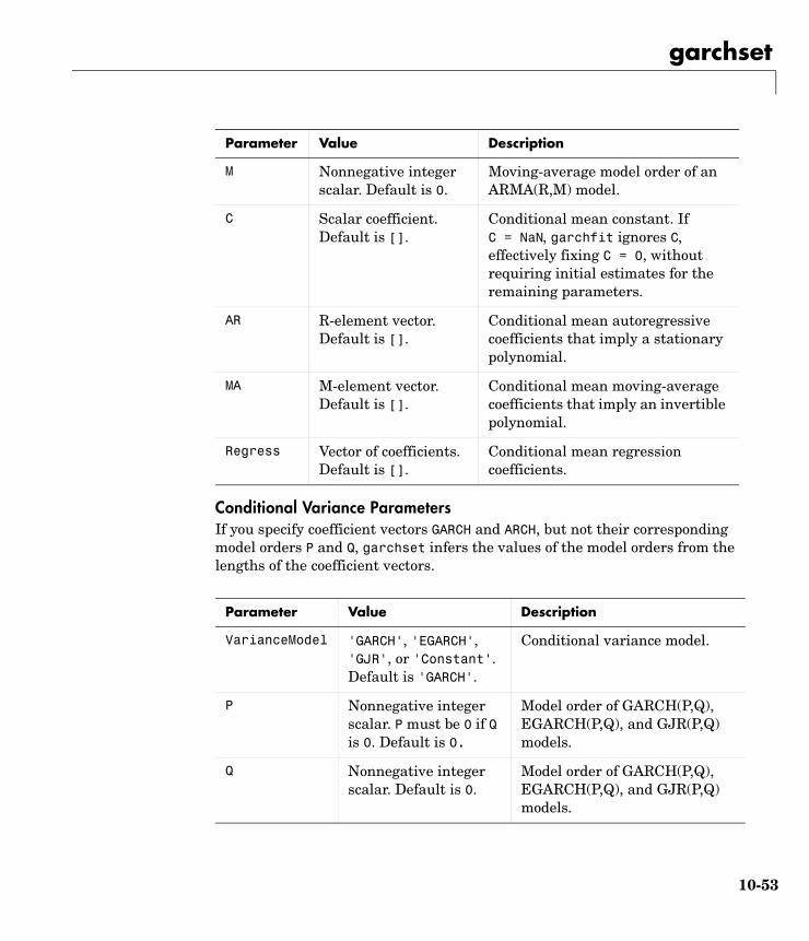
garchset
10-53
Conditional Variance ParametersIf you specify coefficient vectors GARCH and ARCH, but not their corresponding model orders P and Q, garchset infers the values of the model orders from the lengths of the coefficient vectors.
M Nonnegative integer scalar. Default is 0.
Moving-average model order of an ARMA(R,M) model.
C Scalar coefficient. Default is [].
Conditional mean constant. If C = NaN, garchfit ignores C, effectively fixing C = 0, without requiring initial estimates for the remaining parameters.
AR R-element vector. Default is [].
Conditional mean autoregressive coefficients that imply a stationary polynomial.
MA M-element vector. Default is [].
Conditional mean moving-average coefficients that imply an invertible polynomial.
Regress Vector of coefficients. Default is [].
Conditional mean regression coefficients.
Parameter Value Description
VarianceModel 'GARCH', 'EGARCH', 'GJR', or 'Constant'. Default is 'GARCH'.
Conditional variance model.
P Nonnegative integer scalar. P must be 0 if Q is 0. Default is 0.
Model order of GARCH(P,Q), EGARCH(P,Q), and GJR(P,Q) models.
Q Nonnegative integer scalar. Default is 0.
Model order of GARCH(P,Q), EGARCH(P,Q), and GJR(P,Q) models.
Parameter Value Description

garchset
10-54
Equality Constraint ParametersThese parameters are used only by garchfit during estimation. Use these parameters cautiously. The problem can experience difficulty converging if the fixed value is not well suited to the data at hand.
K Scalar coefficient. Default is [].
Conditional variance constant.
GARCH P-element vector. Default is [].
Coefficients related to lagged conditional variances.
ARCH Q-element vector. Default is [].
Coefficients related to lagged innovations (i.e., residuals).
Leverage Q-element vector. Default is [].
Leverage coefficients for asymmetric EGARCH(P,Q) and GJR(P,Q) models.
Parameter Value Description
FixDoF Logical scalar. Default is [].
Equality constraint indicator for DoF parameter.
FixC Logical scalar. Default is [].
Equality constraint indicator for C constant.
FixAR R-element logical vector. Default is [].
Equality constraint indicator for AR coefficients.
FixMA M-element logical vector. Default is [].
Equality constraint indicator for MA coefficients.
FixRegress Logical vector. Default is [].
Equality constraint indicator for the REGRESS coefficients.
FixK Logical scalar. Default is [].
Equality constraint indicator for the K constant.
Parameter Value Description

garchset
10-55
Optimization Parametersgarchfit uses these parameters in calling the Optimization Toolbox function fmincon during estimation.
Examples This example creates a GARCH(1,1) model, then changes it to a GARCH(1,2) model. In each case, it displays the relevant fields in the specification structure. Use garchget to retrieve the values of individual fields.
FixGARCH P-element logical vector. Default is [].
Equality constraint indicator for the GARCH coefficients.
FixARCH Q-element logical vector. Default is [].
Equality constraint indicator for the ARCH coefficients.
FixLeverage Q-element logical vector. Default is [].
Equality constraint indicator for Leverage coefficients.
Parameter Value Description
Display 'on' or 'off'. Default is 'on'.
Display iterative optimization information.
MaxFunEvals Positive integer. Default = (100*number of estimated parameters).
Maximum number of objective function evaluations allowed.
MaxIter Positive integer. Default is 400.
Maximum number of iterations allowed.
TolCon Positive scalar. Default is 1e-007.
Termination tolerance on the constraint violation.
TolFun Positive scalar. Default is 1e-006.
Termination tolerance on the objective function value.
TolX Positive scalar. Default is 1e-006.
Termination tolerance on parameter estimates.
Parameter Value Description

garchset
10-56
spec = garchset('P',1,'Q',1) % Create a GARCH(P=1,Q=1) model.
spec =
Comment: 'Mean: ARMAX(0,0,?); Variance: GARCH(1,1)' Distribution: 'Gaussian' C: [] VarianceModel: 'GARCH' P: 1 Q: 1 K: [] GARCH: [] ARCH: []
spec = garchset(spec,'Q',2) % Change it to a GARCH(P=1,Q=2) % model.spec =
Comment: 'Mean: ARMAX(0,0,?); Variance: GARCH(1,2)' Distribution: 'Gaussian' C: [] VarianceModel: 'GARCH' P: 1 Q: 2 K: [] GARCH: [] ARCH: []
See Also garchfit, garchget, garchpred, garchsim
fmincon (in the Optimization Toolbox)

garchsim
10-57
10garchsimPurpose Univariate GARCH process simulation
Syntax [Innovations,Sigmas,Series] = garchsim(Spec)[...] = garchsim(Spec,NumSamples,NumPaths)[...] = garchsim(Spec,NumSamples,NumPaths,Seed)[...] = garchsim(Spec,NumSamples,NumPaths,Seed,X)[...] = garchsim(Spec,NumSamples,NumPaths,Seed,X,Tolerance)[...] = garchsim(Spec,NumSamples,NumPaths,Seed,X,Tolerance,... PreInnovations,PreSigmas,PreSeries)
Description [Innovations,Sigmas,Series] = garchsim(Spec), given specifications for the conditional mean and variance of a univariate time series, simulates a sample path with 100 observations for the return series, innovations, and conditional standard deviation processes. The conditional mean can be of general ARMAX form and the conditional variance of general GARCH, EGARCH, or GJR form.
[...] = garchsim(Spec,NumSamples,NumPaths) simulates NumPaths sample paths. Each path is sampled at NumSamples observations.
[...] = garchsim(Spec,NumSamples,NumPaths,Seed) specifies a scalar random number generator seed.
[...] = garchsim(Spec,NumSamples,NumPaths,Seed,X) also accepts a time-series regression matrix X of observed explanatory data. garchsim treats each column of X as an individual time series, and uses it as an explanatory variable in the regression component of the conditional mean.
[...] = garchsim(Spec,NumSamples,NumPaths,Seed,X,Tolerance) also accepts a scalar transient response tolerance, such that Tolerance > 0 and ≤ 1. garchsim estimates the number of observations needed for the magnitude of the impulse response, which begins at 1, to decay below the Tolerance value. The number of observations associated with the transient decay period is subject to a maximum of 10,000 to prevent out-of-memory conditions. Tolerance is ignored when you specify presample observations (PreInnovations, PreSigmas, and PreSeries).
Use Tolerance to manage the conflict between transient minimization and memory usage. Smaller Tolerance values generate output processes that more

garchsim
10-58
closely approximate true steady-state behavior, but require more memory for the additional filtering required. Conversely, larger Tolerance values require less memory, but produce outputs in which transients tend to persist.
If you do not explicitly specify presample data (see below), the impulse response estimates are based on the magnitude of the largest eigenvalue of the autoregressive polynomial.
[...] = garchsim(Spec,NumSamples,NumPaths,Seed,X,Tolerance,...PreInnovations,PreSigmas,PreSeries) uses presample observations, contained in the time-series matrices or column vectors PreInnovations, PreSigmas, and PreSeries, to simulate the outputs Innovations, Sigmas, and Series, respectively. When specified, these presample arrays are used to initiate the filtering process, and thus form the conditioning set upon which the simulated realizations are based.
If you specify the presample data as matrices, they must have NumPaths columns. garchsim uses the presample information from a given column to initiate the simulation of the corresponding column of the Innovations, Sigmas, and Series outputs. If you specify the presample data as column vectors, the vectors are applied to each column of the corresponding Innovations, Sigmas, and Series outputs.
If you provide no explicit presample data, the necessary presample observations are derived automatically (see “Automatic Minimization of Transient Effects” on page 4-6.
PreInnovations and PreSigmas are usually companion inputs. Although both are optional, when specified, they are typically entered together. A notable exception would be a GARCH(0,Q) (i.e., an ARCH(Q)) model in which the conditional variance equation does not require lagged conditional variance forecasts. Similarly, PreSeries is only necessary when you want to simulate the output return Series, and when the conditional mean equation has an autoregressive component.
If the conditional mean or the conditional variance equation (“Conditional Mean and Variance Models” on page 2-6) is not recursive in any way, then certain presample information is unnecessary to jump-start the models. However, specifying redundant presample information is not an error, and garchsim ignores any presample observations you specify for models that require no such information.

garchsim
10-59
Input Arguments
Spec GARCH specification structure for the conditional mean and variance models. You create Spec by calling the function garchset or the estimation function garchfit. The conditional mean can be of general ARMAX form and the conditional variance of general GARCH form.
NumSamples (optional) Positive integer indicating the number of observations garchsim generates for each path of the Innovations, Sigmas, and Series outputs. If NumSamples = [] or is not specified, the default is 100.
NumPaths (optional) Positive integer indicating the number of sample paths (realizations) garchsim generates for the Innovations, Sigmas, and Series outputs. If NumPaths = [] or is not specified, the default is 1; i.e. Innovations, Sigmas and Series are column vectors.
PreInnovations Time-series matrix or column vector of presample innovations on which the recursive mean and variance models are conditioned. This array can have any number of rows, provided it contains sufficient observations to initialize the mean and variance equations. I.e., if M and Q are the number of lagged innovations required by the conditional mean and variance equations, respectively, then PreInnovations must have at least max(M,Q) rows.
If the number of rows exceeds max(M,Q), then only the last (i.e., most recent) max(M,Q) rows are used. If PreInnovations is a matrix, then it must have NumPaths columns.

garchsim
10-60
PreSigmas Time-series matrix or column vector of positive presample conditional standard deviations on which the recursive variance model is conditioned. This array can have any number of rows, provided it contains sufficient observations to initialize the conditional variance equation. I.e., if P and Q are the number of lagged conditional standard deviations and lagged innovations required by the conditional variance equation, respectively, then PreSigmas must have at least P rows for GARCH and GJR models, and at least max(P,Q) rows for EGARCH models.
If the number of rows exceeds the requirement, then only the last (i.e., most recent) rows are used. If PreSigmas is a matrix, then it must have NumPaths columns.
PreSeries Time-series matrix or column vector of presample observations of the return series of interest on which the recursive mean model is conditioned. This array can have any number of rows, provided it contains sufficient observations to initialize the conditional mean equation. Thus, if R is the number of lagged observations of the return series required by the conditional mean equation, then PreSeries must have at least R rows. If the number of rows exceeds R, then only the last (i.e., most recent) R rows are used. If PreSeries is a matrix, then it must have NumPaths columns.
Seed Scalar random number generator seed. It corresponds to the rand and randn syntaxes, rand('state',j) and randn('state',j). If Seed = [] or is not specified, the default is 0 (the MATLAB initial state).
Tolerance Scalar transient response tolerance, such that 0 < Tolerance <= 1. This tolerance parameter is ignored if presample conditioning information has been specified (see PreInnovations, PreSigmas, and PreSeries). If empty or missing, the default is 0.01 (i.e., 1%).

garchsim
10-61
Output Arguments
Examples See “Simulating Sample Paths” on page 4-2, “Fitting a Model to a Simulated Return Series” on page 7-3, and “Monte Carlo Simulation” on page 9-6.
See Also garchfit, garchget, garchpred, garchset
X Time-series regression matrix of observed explanatory data. Typically, X is a matrix of asset returns (e.g., the return series of an equity index), and represents the past history of the explanatory data. Each column of X is an individual time series used as an explanatory variable in the regression component of the conditional mean. In each column, the first row contains the oldest observation and the last row the most recent.
If X = [] or is not specified, the conditional mean has no regression component. If specified, then at least the most recent NumSamples observations of each return series must be valid (i.e., non-NaN). When the number of valid observations in each series exceeds NumSamples, garchsim uses only the most recent NumSamples observations of X.
Innovations NumSamples by NumPaths matrix of innovations, representing a mean zero, discrete-time stochastic process. The Innovations time series follows the conditional variance specification defined in Spec. Rows are sequential observations, columns are realizations.
Sigmas NumSamples by NumPaths matrix of conditional standard deviations of the corresponding Innovations matrix. Innovations and Sigmas are the same size. Rows are sequential observations. Columns are realizations.
Series NumSamples by NumPaths matrix of the return series of interest. Series is the dependent stochastic process and follows the conditional mean specification of general ARMAX form defined in Spec. Rows are sequential observations. Columns are realizations.

garchsim
10-62
References [1] Bollerslev, T., “A Conditionally Heteroskedastic Time Series Model for Speculative Prices and Rates of Return,” Review of Economics and Statistics, Vol. 69, 1987, pp 542-547.
[2] Bollerslev, T., “Generalized Autoregressive Conditional Heteroskedasticity,” Journal of Econometrics, Vol. 31, 1986, pp 307-327.
[3] Box, G.E.P., G.M. Jenkins, and G.C. Reinsel, Time Series Analysis: Forecasting and Control, Third edition, Prentice Hall, 1994.
[4] Enders, W., Applied Econometric Time Series, John Wiley & Sons, 1995.
[5] Engle, Robert, “Autoregressive Conditional Heteroskedasticity with Estimates of the Variance of United Kingdom Inflation,” Econometrica, Vol. 50, 1982, pp 987-1007.
[6] Engle, R.F., D.M. Lilien, and R.P. Robins, “Estimating Time Varying Risk Premia in the Term Structure: The ARCH-M Model,” Econometrica, Vol. 59,1987, pp 391-407.
[7] Glosten, L.R., R. Jagannathan, and D.E. Runkle, “On the Relation Between Expected Value and the Volatility of the Nominal Excess Return on Stocks,” The Journal of Finance, Vol.48, 1993, pp 1779-1801.
[8] Hamilton, J.D., Time Series Analysis, Princeton University Press, 1994.
[9] Nelson, D.B., “Conditional Heteroskedasticity in Asset Returns: A New Approach,” Econometrica, Vol. 59, 1991, pp 347-370.

lagmatrix
10-63
10lagmatrixPurpose Create a lagged time-series matrix
Syntax XLAG = lagmatrix(X,Lags)
Description XLAG = lagmatrix(X,Lags) creates a lagged (i.e., shifted) version of a time-series matrix. The lagmatrix function is useful for creating a regression matrix of explanatory variables for fitting the conditional mean of a return series.
Input Arguments
Output Arguments
Examples Example 1. The following example creates a bivariate time-series matrix X with five observations each, then creates a lagged matrix XLAG composed of X and the first two lags of X. The result, XLAG, is a 5-by-6 matrix.
X Time-series of explanatory data. X can be a column vector or a matrix. As a column vector, X represents a univariate time series whose first element contains the oldest observation and whose last element contains the most recent observation. As a matrix, X represents a multivariate time series whose rows correspond to time indices in which the first row contains the oldest observations and the last row contains the most recent observations. lagmatrix assumes that observations across any given row occur at the same time. Each column is an individual time series.
Lags Vector of integer lags. lagmatrix applies the first lag to every series in X, then applies the second lag to every series in X, and so forth. To include a time series as is, include a 0 lag. Positive lags correspond to delays, and shift a series back in time. Negative lags correspond to leads, and shift a series forward in time.
XLAG Lagged transform of the time series X. To create XLAG, lagmatrix shifts each time series in X by the first lag, then shifts each time series in X by the second lag, and so forth. Since XLAG represents an explanatory regression matrix, each column is an individual time series. XLAG has the same number of rows as there are observations in X, but its column dimension is equal to the product of the number of columns in X and the length of Lags. lagmatrix uses a NaN (Not-a-Number) to indicate an undefined observation.

lagmatrix
10-64
X = [1 -1; 2 -2 ;3 -3 ;4 -4 ;5 -5] % Create a simple bivariate % series.X = 1 -1 2 -2 3 -3 4 -4 5 -5
XLAG = lagmatrix(X,[0 1 2]) % Create the lagged matrix.
XLAG = 1 -1 NaN NaN NaN NaN 2 -2 1 -1 NaN NaN 3 -3 2 -2 1 -1 4 -4 3 -3 2 -2 5 -5 4 -4 3 -3
Example 2. See “Fitting a Regression Model to the Same Return Series” on page 7-5 for another example.
See Also filter, isnan, and nan (all in MATLAB)

lbqtest
10-65
10lbqtestPurpose Ljung-Box Q-statistic lack-of-fit hypothesis test
Syntax [H,pValue,Qstat,CriticalValue] = lbqtest(Series,Lags,Alpha,DoF)
Description [H,pValue,Qstat,CriticalValue] = lbqtest(Series,Lags,Alpha,DoF)performs the Ljung-Box lack-of-fit hypothesis test for model misspecification, which is based on the Q-statistic
where = sample size, = number of autocorrelation lags included in the statistic, and is the squared sample autocorrelation at lag . Once you fit a univariate model to an observed time series, you can use the Q-statistic as a lack-of-fit test for a departure from randomness. Under the null hypothesis that the model fit is adequate, the test statistic is asymptotically chi-square distributed.
Input Arguments
Q N N 2+( )rk
2
N k–( )-------------------
k 1=
L
∑=
N Lrk
2 k
Series Vector of observations of a univariate time series for which lbqtest computes the sample Q-statistic. The last row of Series contains the most recent observation of the stochastic sequence. Typically, Series is either the sample residuals derived from fitting a model to an observed time series, or the standardized residuals obtained by dividing the sample residuals by the conditional standard deviations.
Lags Vector of positive integers indicating the lags of the sample autocorrelation function included in the Q-statistic. If specified, each lag must be less than the length of Series. If Lags = [] or is not specified, the default is Lags = min([20, length(Series)-1]).
Alpha Significance levels. Alpha can be a scalar applied to all lags, or a vector the same length as Lags. If Alpha = [] or is not specified, the default is 0.05. For all elements, , of Alpha, .α 0 α 1< <

lbqtest
10-66
Output Arguments
Examples Example 1. Create a vector of 100 Gaussian random numbers, then compute the Q-statistic for autocorrelation lags 20 and 25 at the 10 percent significance level.
randn('state',100) % Start from a known state.Series = randn(100,1); % 100 Gaussian deviates ~ N(0,1)[H,P,Qstat,CV] = lbqtest(Series, [20 25]', 0.10);[H,P,Qstat,CV]
ans = 0 0.9615 10.3416 28.4120 0 0.9857 12.1015 34.3816
Example 2. See “Preestimation Analysis” on page 2-15 for another example.
See Also archtest, autocorr
DoF Degrees of freedom. DoF can be a scalar applied to all lags, or a vector the same length as Lags. If specified, all elements of DoF must be positive integers less than the corresponding element of Lags. If DoF = [] or is not specified, the elements of Lags serve as the default degrees of freedom for the chi-square distribution.
H Boolean decision vector. 0 indicates acceptance of the null hypothesis that the model fit is adequate (no serial correlation at the corresponding element of Lags). 1 indicates rejection of the null hypothesis. H is the same size as Lags.
pValue Vector of P-values (significance levels) at which lbqtest rejects the null hypothesis of no serial correlation at each lag in Lags.
Qstat Vector of Q-statistics for each lag in Lags.
CriticalValue Vector of critical values of the chi-square distribution for comparison with the corresponding element of Qstat.

lbqtest
10-67
References [1] Box, G.E.P., G.M. Jenkins, and G.C. Reinsel, Time Series Analysis: Forecasting and Control, Third edition, Prentice Hall, 1994.
[2] Gourieroux, C., ARCH Models and Financial Applications, Springer-Verlag, 1997.

lratiotest
10-68
10lratiotestPurpose Likelihood ratio hypothesis test
Syntax [H,pValue,Ratio,CriticalValue] = lratiotest(BaseLLF,NullLLF,... DoF,Alpha)
Description [H,pValue,Ratio,CriticalValue] = lratiotest(BaseLLF,NullLLF,DoF,Alpha) performs the likelihood ratio hypothesis test. lratiotest uses as input the optimized log-likelihood objective function (LLF) value associated with an unrestricted maximum likelihood parameter estimate, and the LLF values associated with restricted parameter estimates.
The unrestricted LLF is the baseline case used to fit conditional mean and variance specifications to an observed univariate return series. The restricted models determine the null hypotheses of each test, and the number of restrictions they impose determines the degrees of freedom of the resulting chi-square distribution.
BaseLLF is usually the LLF of a larger estimated model and serves as the alternative hypothesis. Elements of NullLLF are then the LLFs associated with smaller, restricted specifications. BaseLLF should exceed the values in NullLLF, and the asymptotic distribution of the test statistic is chi-square distributed with degrees of freedom equal to the number of restrictions.
Input Arguments
BaseLLF Scalar value of the optimized log-likelihood objective function of the baseline, unrestricted estimate. lratiotest assumes BaseLLF is the output of the estimation function garchfit or the inference function garchinfer.
NullLLF Vector of optimized log-likelihood objective function values of the restricted estimates. lratiotest assumes you obtained the NullLLF values using garchfit or garchinfer.
DoF Degrees of freedom (i.e., the number of parameter restrictions) associated with each value in NullLLF. DoF can be a scalar applied to all values in NullLLF, or a vector the same length as NullLLF. All elements of DoF must be positive integers.

lratiotest
10-69
Output Arguments
Examples See “Likelihood Ratio Tests” on page 8-2 and “Equality Constraints and Parameter Significance” on page 8-7.
See Also garchfit, garchinfer
References [1] Hamilton, J.D., Time Series Analysis, Princeton University Press, 1994.
Alpha Significance levels of the hypothesis test. Alpha can be a scalar applied to all values in NullLLF, or a vector the same length as NullLLF. If Alpha = [] or is not specified, the default is 0.05. For all elements, , of Alpha, .α 0 α 1< <
H Vector of Boolean decisions the same size as NullLLF. A 0 indicates acceptance of the restricted model under the null hypothesis. 1 indicates rejection of the restricted, null hypothesis model relative to the unrestricted alternative associated with BaseLLF.
pValue Vector of P-values (significance levels) at which lratiotest rejects the null hypothesis of each restricted model. pValue is the same size as NullLLF.
Ratio Vector of likelihood ratio test statistics the same size as NullLLF. The test statistic is
CriticalValue Vector of critical values of the chi-square distribution. CriticalValue is the same size as NullLLF.
Ratio 2 BaseLLF NullLLF–( )=
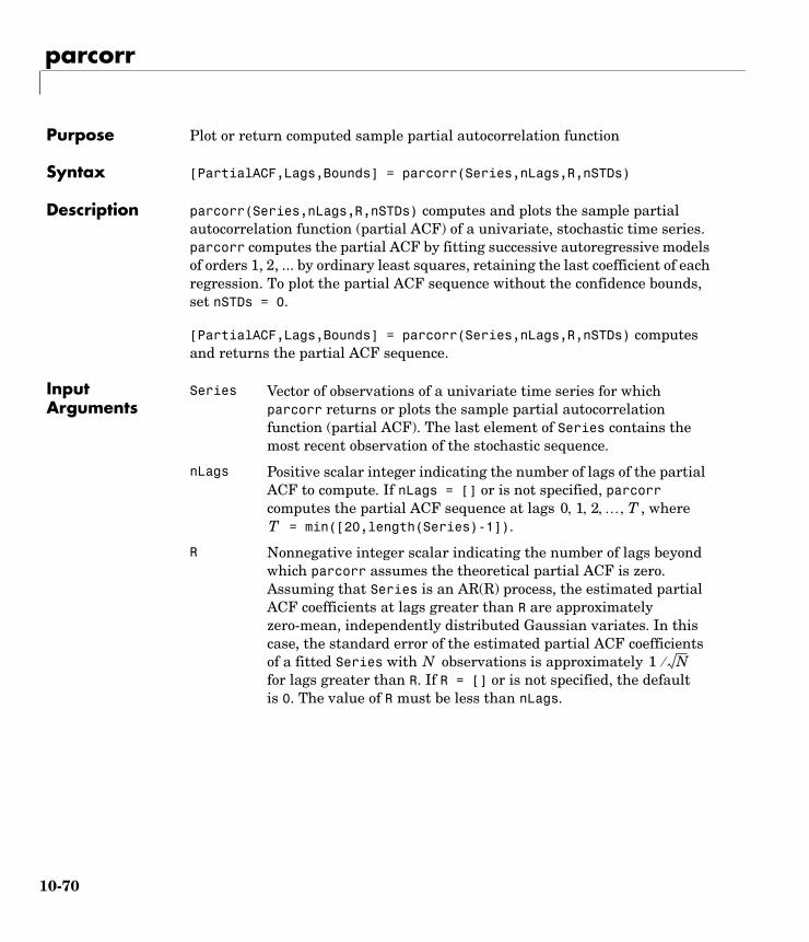
parcorr
10-70
10parcorrPurpose Plot or return computed sample partial autocorrelation function
Syntax [PartialACF,Lags,Bounds] = parcorr(Series,nLags,R,nSTDs)
Description parcorr(Series,nLags,R,nSTDs) computes and plots the sample partial autocorrelation function (partial ACF) of a univariate, stochastic time series. parcorr computes the partial ACF by fitting successive autoregressive models of orders 1, 2, ... by ordinary least squares, retaining the last coefficient of each regression. To plot the partial ACF sequence without the confidence bounds, set nSTDs = 0.
[PartialACF,Lags,Bounds] = parcorr(Series,nLags,R,nSTDs) computes and returns the partial ACF sequence.
Input Arguments
Series Vector of observations of a univariate time series for which parcorr returns or plots the sample partial autocorrelation function (partial ACF). The last element of Series contains the most recent observation of the stochastic sequence.
nLags Positive scalar integer indicating the number of lags of the partial ACF to compute. If nLags = [] or is not specified, parcorr computes the partial ACF sequence at lags , where
= min([20,length(Series)-1]).
R Nonnegative integer scalar indicating the number of lags beyond which parcorr assumes the theoretical partial ACF is zero. Assuming that Series is an AR(R) process, the estimated partial ACF coefficients at lags greater than R are approximately zero-mean, independently distributed Gaussian variates. In this case, the standard error of the estimated partial ACF coefficients of a fitted Series with observations is approximately for lags greater than R. If R = [] or is not specified, the default is 0. The value of R must be less than nLags.
0 1 2 … T, , , ,T
N 1 N⁄

parcorr
10-71
Output Arguments
Examples Example 1. Create a stationary AR(2) process from a sequence of 1000 Gaussian deviates, and then visually assess whether the partial ACF is zero for lags greater than 2.
randn('state',0) % Start from a known state.x = randn(1000,1); % 1000 Gaussian deviates ~ N(0,1).y = filter(1,[1 -0.6 0.08],x); % Create a stationary AR(2) % process.[PartialACF,Lags,Bounds] = parcorr(y,[],2); % Compute the % partial ACF with 95 percent % confidence.[Lags,PartialACF]
nSTDs Positive scalar indicating the number of standard deviations of the sample partial ACF estimation error to display, assuming that Series is an AR(R) process. If the Rth regression coefficient (i.e., the last ordinary least squares (OLS) regression coefficient of Series regressed on a constant and R of its lags) includes observations, specifying nSTDs results in confidence bounds at
. If nSTDs = [] or is not specified, the default is 2 (i.e., approximate 95 percent confidence interval).
N
nSTDs N⁄( )±
PartialACF Sample partial ACF of Series. PartialACF is a vector of length nLags + 1 corresponding to lags 0, 1, 2, ..., nLags. The first element of PartialACF is unity, i.e., PartialACF(1) = 1 = OLS regression coefficient of Series regressed upon itself. parcorr includes this element as a reference.
Lags Vector of lags, of length nLags + 1. The elements correspond to the elements of PartialACF.
Bounds Two-element vector indicating the approximate upper and lower confidence bounds, assuming that Series is an AR(R) process. Note that Bounds is approximate for lags greater than R only.

parcorr
10-72
ans = 0 1.0000 1.0000 0.5570 2.0000 -0.0931 3.0000 0.0249 4.0000 -0.0180 5.0000 -0.0099 6.0000 0.0483 7.0000 0.0058 8.0000 0.0354 9.0000 0.0623 10.0000 0.0052 11.0000 -0.0109 12.0000 0.0421 13.0000 -0.0086 14.0000 -0.0324 15.0000 0.0482 16.0000 0.0008 17.0000 -0.0192 18.0000 0.0348 19.0000 -0.0320 20.0000 0.0062
Bounds
Bounds = 0.0633 -0.0633
parcorr(y,[],2) % Use the same example, but plot % the partial ACF sequence with % confidence bounds.

parcorr
10-73
Example 2. See “Preestimation Analysis” on page 2-15 for another example.
See Also autocorr, crosscorrfilter (MATLAB)
References [1] Box, G.E.P., G.M. Jenkins, and G.C. Reinsel, Time Series Analysis: Forecasting and Control, Third edition, Prentice Hall, 1994.
[2] Hamilton, J.D., Time Series Analysis, Princeton University Press, 1994.
0 5 10 15 20−0.2
0
0.2
0.4
0.6
0.8
Lag
Sam
ple
Par
tial A
utoc
orre
latio
ns
Sample Partial Autocorrelation Function

price2ret
10-74
10price2retPurpose Convert a price series to a return series
Syntax [RetSeries,RetIntervals] = price2ret(TickSeries,TickTimes,Method)
Description [RetSeries,RetIntervals] = price2ret(TickSeries,TickTimes,Method)computes asset returns for NUMOBS price observations of NUMASSETS assets.
Input Arguments
TickSeries Time series of price data. TickSeries can be a column vector or a matrix:
• As a vector, TickSeries represents a univariate price series. The length of the vector is the number of observations (NUMOBS). The first element contains the oldest observation, and the last element the most recent.
• As a matrix, TickSeries represents a NUMOBS-by-number of assets (NUMASSETS) matrix of asset prices. Rows correspond to time indices. The first row contains the oldest observations and the last row the most recent. price2ret assumes that the observations across a given row occur at the same time for all columns, and each column is a price series of an individual asset.
TickTimes A NUMOBS element vector of monotonically increasing observation times. Times are numeric and taken either as serial date numbers (day units), or as decimal numbers in arbitrary units (e.g., yearly). If TickTimes = [] or is not specified, then price2ret assumes sequential observation times from 1, 2, ..., NUMOBS.
Method Character string indicating the compounding method to compute asset returns. If Method = 'Continuous', = [], or is not specified, then price2ret computes continuously compounded returns. If Method = 'Periodic', then price2ret assumes simple periodic returns. Method is case insensitive.

price2ret
10-75
Output Arguments
Examples Create a stock price process continuously compounded at 10 percent, then convert the price series to a 10 percent return series.
S = 100*exp(0.10 * [0:19]'); % Create the stock price seriesR = price2ret(S); % Convert the price series to a 10 percent % return series
RetSeries Array of asset returns:
• When TickSeries is a NUMOBS element column vector, RetSeries is a NUMOBS-1 column vector.
• When TickSeries is a NUMOBS-by-NUMASSETS matrix, RetSeries is a (NUMOBS-1)-by-NUMASSETS matrix. price2ret quotes the th return of an asset for the period TickTimes(i) to TickTimes(i+1) and normalizes it by the time interval between successive price observations.
Assuming that
then if Method = 'Continuous', = [], or is not specified, price2ret computes the continuously compounded th return of an asset as
If Method = 'Periodic', then price2ret computes the th simple return as
RetIntervals NUMOBS-1 element vector of interval times between observations. If TickTimes = [] or is not specified, price2ret assumes that all intervals are 1.
i
RetIntervals i( ) TickTimes i 1+( ) TickTimes i( )–=
i
RetSeries i( )
TickSeries i 1+( )TickSeries i( )
----------------------------------------------------log
RetIntervals i( )-------------------------------------------------------------------=
i
RetSeries i( )
TickSeries i 1+( )TickSeries i( )
---------------------------------------------------- 1–
RetIntervals i( )-------------------------------------------------------------------=

price2ret
10-76
[S [R;NaN]] % Pad the return series so vectors are of same % length. price2ret computes the ith return from % the ith and i+1th prices.
ans =
100.0000 0.1000 110.5171 0.1000 122.1403 0.1000 134.9859 0.1000 149.1825 0.1000 164.8721 0.1000 182.2119 0.1000 201.3753 0.1000 222.5541 0.1000 245.9603 0.1000 271.8282 0.1000 300.4166 0.1000 332.0117 0.1000 366.9297 0.1000 405.5200 0.1000 448.1689 0.1000 495.3032 0.1000 547.3947 0.1000 604.9647 0.1000 668.5894 NaN
See Also ret2price

ret2price
10-77
10ret2pricePurpose Convert a return series to a price series
Syntax [TickSeries,TickTimes] = ret2price(RetSeries,StartPrice,... RetIntervals,StartTime,Method)
Description [TickSeries,TickTimes] = ret2price(RetSeries,StartPrice,RetIntervals,StartTime,Method)generates price series for the specified assets, given the asset starting prices and the return observations for each asset.
Input Arguments
RetSeries Time-series array of returns. RetSeries can be a column vector or a matrix:
• As a vector, RetSeries represents a univariate series of returns of a single asset. The length of the vector is the number of observations (NUMOBS). The first element contains the oldest observation, and the last element the most recent.
• As a matrix, RetSeries represents a NUMOBS-by-number of assets (NUMASSETS) matrix of asset returns. Rows correspond to time indices. The first row contains the oldest observations and the last row the most recent. ret2price assumes that the observations across a given row occur at the same time for all columns, and each column is a return series of an individual asset.
StartPrice A NUMASSETS element vector of initial prices for each asset, or a single scalar initial price applied to all assets. If StartPrice = [] or is not specified, all asset prices start at 1.
RetIntervals A NUMOBS element vector of time intervals between return observations, or a single scalar interval applied to all observations. If RetIntervals = [] or is not specified, ret2price assumes all intervals have length 1.
StartTime (optional) Scalar starting time for the first observation, applied to the price series of all assets. The default is 0.

ret2price
10-78
Output Arguments
Examples Example 1. Create a stock price process continuously compounded at 10 percent. Compute 10 percent returns for reference, then convert the resulting return series to the original price series and compare results.
S = 100*exp(0.10 * [0:19]'); % Create the stock price seriesR = price2ret(S); % Convert the price series to a % 10 percent return seriesP = ret2price(R,100); % Convert to the original price % series[S P] % Compare the original and % computed price series
ans =
100.0000 100.0000 110.5171 110.5171 122.1403 122.1403 134.9859 134.9859
Method Character string indicating the compounding method used to compute asset returns. If Method = 'Continuous', = [], or is not specified, then ret2price computes continuously compounded returns. If Method = 'Periodic' then ret2price computes simple periodic returns. Method is case insensitive.
TickSeries Array of asset prices:
• When RetSeries is a NUMOBS element column vector, TickSeries is a NUMOBS+1 column vector. The first element contains the starting price of the asset, and the last element the most recent price.
• When RetSeries is a NUMOBS-by-NUMASSETS matrix, then RetSeries is a (NUMOBS+1)-by-NUMASSETS matrix. The first row contains the starting price of the assets, and the last row contains the most recent prices.
TickTimes A NUMOBS+1 element vector of price observation times. The initial time is zero unless specified in StartTime.

ret2price
10-79
149.1825 149.1825 164.8721 164.8721 182.2119 182.2119 201.3753 201.3753 222.5541 222.5541 245.9603 245.9603 271.8282 271.8282 300.4166 300.4166 332.0117 332.0117 366.9297 366.9297 405.5200 405.5200 448.1689 448.1689 495.3032 495.3032 547.3947 547.3947 604.9647 604.9647 668.5894 668.5894
Example 2. This example compares the relative price performance of the Nasdaq and the NYSE indexes (see “Data Sets” on page 1-11). Before plotting the series, the example converts the prices to returns, then converts them back to prices specifying the same starting price, 100, for each series. In the plot, the blue (upper) plot shows the NASDAQ price series, the green (lower) plot shows the NYSE price series.
load garchdatanasdaq = price2ret(NASDAQ);nyse = price2ret(NYSE);plot(ret2price(price2ret([NASDAQ NYSE]),100))ylabel('Prices')legend('Nasdaq','NYSE',2)

ret2price
10-80
See Also price2ret
0 500 1000 1500 2000 2500 3000 35000
2
4
6
8
10
12
Pric
es
NasdaqNYSE

A
Glossary

A Glossary
A-2
Akaike information criteria (AIC) – A model-order selection criterion based on parsimony. More complicated models are penalized for the inclusion of additional parameters. See also Bayesian information criteria.
AR – Autoregressive. AR models include past observations of the dependent variable in the forecast of future observations.
ARCH – Autoregressive Conditional Heteroscedasticity. A time-series technique in which past observations of the variance are used to forecast future variances. See also GARCH.
ARMA – Autoregressive Moving Average. A time-series model that includes both AR and MA components. See also AR and MA.
autocorrelation function (ACF) – Correlation sequence of a random time series with itself. See also crosscorrelation function.
autoregressive – See AR.
Bayesian information criteria (BIC) – A model-order selection criterion based on parsimony. More complicated models are penalized for the inclusion of additional parameters. Since BIC imposes a greater penalty for additional parameters than AIC, BIC always provides a model with a number of parameters no greater than that chosen by AIC. See also Akaike information criteria.
conditional – Time-series technique with explicit dependence on the past sequence of observations.
conditional mean – Time-series model for forecasting the expected value of the return series itself.
conditional variance – Time-series model for forecasting the expected value of the variance of the return series.
crosscorrelation function (XCF) – Correlation sequence between two random time series. See also autocorrelation function.
equality constraint – A constraint, imposed during parameter estimation, by which a parameter is held fixed at a user-specified value.
excess kurtosis – A characteristic, relative to a standard normal probability distribution, whereby an area under the probability density function is reallocated from the center of the distribution to the tails (fat tails). Samples obtained from distributions with excess kurtosis have a higher probability of

A-3
containing outliers than samples drawn from a normal (Gaussian) density. Time series that exhibit a fat tail distribution are often referred to as leptokurtic.
explanatory variables – Time series used to explain the behavior of another observed series of interest. Explanatory variables are typically incorporated into a regression framework.
fat tails – See excess kurtosis.
GARCH – Generalized Autoregressive Conditional Heteroscedasticity. A time-series technique in which past observations of the variance and variance forecast are used to forecast future variances. See also ARCH.
heteroscedasticity – Time-varying, or time-dependent, variance.
homoscedasticity – Time-independent variance. The GARCH Toolbox also refers to homoscedasticity as constant conditional variance.
i.i.d. – Independent, identically distributed.
innovations – A sequence of unanticipated shocks, or disturbances. The GARCH Toolbox uses innovations and residuals interchangeably.
leptokurtic – See excess kurtosis.
MA – Moving average. MA models include past observations of the innovations noise process in the forecast of future observations of the dependent variable of interest.
MMSE – Minimum mean square error. A technique designed to minimize the variance of the estimation or forecast error. See also RMSE.
moving average – See MA.
objective function – The function to be numerically optimized. In the GARCH Toolbox, the objective function is the log-likelihood function of a random process.
partial autocorrelation function (PACF) – Correlation sequence estimated by fitting successive order autoregressive models to a random time series by least squares. The PACF is useful for identifying the order of an autoregressive model.
path – A random trial of a time-series process.
P-value – The lowest level of significance at which a test statistic is significant.

A Glossary
A-4
realization – See path.
residuals – See innovations.
RMSE – Root mean square error. The square root of the mean square error. See also MMSE.
standardized innovations – The innovations divided by the corresponding conditional standard deviation.
time series – Discrete-time sequence of observations of a random process. The type of time series of interest in the GARCH Toolbox is typically a series of returns, or relative changes of some underlying price series.
transient – A response, or behavior, of a time series that is heavily dependent on the initial conditions chosen to begin a recursive calculation. The transient response is typically undesirable, and initially masks the true steady-state behavior of the process of interest.
unconditional – Time-series technique in which explicit dependence on the past sequence of observations is ignored. Equivalently, the time stamp associated with any observation is ignored.
volatility – The risk, or uncertainty, measure associated with a financial time series. The GARCH Toolbox associates volatility with standard deviation.

B
Bibliography

B Bibliography
B-2
[1] Baillie, R.T., and T. Bollerslev, “Prediction in Dynamic Models with Time-Dependent Conditional Variances,” Journal of Econometrics, Vol. 52, 1992, pp 91-113.
[2] Bera, A.K., and H.L. Higgins, “A Survey of ARCH Models: Properties, Estimation and Testing,” Journal of Economic Surveys, Vol. 7, No. 4, 1993.
[3] Bollerslev, T., “A Conditionally Heteroskedastic Time Series Model for Speculative Prices and Rates of Return,” Review of Economics and Statistics, Vol. 69, 1987, pp 542-547.
[4] Bollerslev, T., “Generalized Autoregressive Conditional Heteroskedasticity,” Journal of Econometrics, Vol. 31, 1986, pp 307-327.
[5] Bollerslev, T., R.Y. Chou, and K.F. Kroner, “ARCH Modeling in Finance: A Review of the Theory and Empirical Evidence,” Journal of Econometrics, Vol. 52, 1992, pp 5-59.
[6] Bollerslev, T., R.F. Engle, and D.B. Nelson, “ARCH Models,” Handbook of Econometrics, Volume IV, Chapter 49, pp 2959-3038, Elsevier Science B.V., 1994.
[7] Bollerslev, T., and E. Ghysels, "Periodic Autoregressive Conditional Heteroscedasticity," Journal of Business and Economic Statistics, Vol. 14, 1996, pp 139-151.
[8] Box, G.E.P., G.M. Jenkins, and G.C. Reinsel, Time Series Analysis: Forecasting and Control, Third edition, Prentice Hall, 1994.
[9] Brooks, C., S.P. Burke, and G. Persand, "Benchmarks and the Accuracy of GARCH Model Estimation," International Journal of Forecasting, Vol. 17, 2001, pp 45-56.
[10] Campbell, J.Y., A.W. Lo, and A.C. MacKinlay, "The Econometrics of Financial Markets," Nonlinearities in Financial Data, Chapter 12, Princeton University Press, 1997.
[11] Enders, W., Applied Econometric Time Series, John Wiley & Sons, 1995.
[12] Engle, Robert F., “Autoregressive Conditional Heteroskedasticity with Estimates of the Variance of United Kingdom Inflation,” Econometrica, Vol. 50, 1982, pp 987-1007.

B-3
[13] Engle, Robert F., D.M. Lilien, and R.P. Robins, “Estimating Time Varying Risk Premia in the Term Structure: The ARCH-M Model,” Econometrica, Vol. 59, 1987, pp 391-407.
[14] Glosten, L.R., R. Jagannathan, and D.E. Runkle, “On the Relation between Expected Value and the Volatility of the Nominal Excess Return on Stocks,” The Journal of Finance, Vol. 48, 1993, pp 1779-1801.
[15] Gourieroux, C., ARCH Models and Financial Applications, Springer-Verlag, 1997.
[16] Hagerud, G.E., “Modeling Nordic Stock Returns with Asymmetric GARCH,” Working Paper Series in Economics and Finance, No. 164, Department of Finance, Stockholm School of Economics, 1997. http://netec.mcc.ac.uk/WoPEc/data/Papers/hhshastef0164.html
[17] Hagerud, G.E., “Specification Tests for Asymmetric GARCH,” Working Paper Series in Economics and Finance, No. 163, Department of Finance, Stockholm School of Economics, 1997. http://netec.mcc.ac.uk/WoPEc/data/Papers/hhshastef0163.html
[18] Hamilton, J.D., Time Series Analysis, Princeton University Press, 1994.
[19] Hentschel, L., “All in the Family: Nesting Symmetric and Asymmetric GARCH Models,” Journal of Financial Economics, Vol. 39, 1995, pp 71-104.
[20] Johnson, N.L., S. Kotz, and N. Balakrishnan, Continuous Univariate Distributions, Vol. 2, Second edition, John Wiley & Sons, 1995.
[21] McCullough, B.D., and C.G. Renfro, “Benchmarks and Software Standards: A Case Study of GARCH Procedures,” Journal of Economic and Social Measurement, Vol. 25, 1998, pp 59-71. http://qed.econ.queensu.ca/faculty/mackinnon/econ872/papers/mccullough.pdf
[22] Nelson, D.B., “Conditional Heteroskedasticity in Asset Returns: A New Approach,” Econometrica, Vol. 59, 1991, pp 347-370.
[23] Peters, J.P., “Estimating and Forecasting Volatility of Stock Indices Using Asymmetric GARCH Models and Skewed Student-t Densities,” Working Paper, École d'Administration des Affaires, University of Liège, Belgium, March 20, 2001. http://www.panagora.com/2001crowell/2001cp_50.pdf

B Bibliography
B-4

I-1
Index
AACF 10-9AIC
computing 10-5model selection 8-5
aicbic function 10-5Akaike information criteria
computing 10-5model selection 8-5
analysis exampleusing default model 2-15
AR modelconverting from ARMA model 10-17
ARCH/GARCH effectshypothesis test 10-7
archtest function 10-7ARMA model
converting to AR model 10-17converting to MA model 10-37
array size 1-7arrays
time series 1-7asymptotic behavior
for long-range forecast horizons 6-6long-range forecasts 6-6
autocorr function 10-9autocorrelation function 10-9autoregressive model
converting from ARMA model 10-17
BBayesian information criteria
computing 10-5model selection 8-5
BICcomputing 10-5
model selection 8-5
Ccompounding
continuous and periodic 1-8conditional mean models 2-6
regression components 7-2conditional standard deviations
inferred from return series 10-32of forecast errors 10-43simulating 10-55
conditional variance models 2-6conditional variances
constant 7-11constraints
active lower bound example 5-28equality 8-7fixing model parameters 8-7tolerance limits 5-16
conventionstechnical 1-7
convergencedetermining status 5-31tolerance options 5-14
crosscorr function 10-13crosscorrelation function 10-13
Ddata sets 1-11
Deutschmark/British Pound FX price series 1-11
Nasdaq Composite Index 1-12New York Stock Exchange Composite Index
1-12

Index
I-2
defaultGARCH model 2-12
default modelestimation and analysis example 2-15estimation example 2-15
Deutschmark/British Pound FX price series 1-11
distributionssupported 2-4
EEGARCH(P,Q) conditional variance model 2-8Engle’s hypothesis test 10-7equality constraints
initial parameter estimates 8-11parameter significance 8-7
estimation 5-1advanced example 9-2control of optimization process 5-13convergence 5-14count of coefficients 8-5, 10-20incorporating a regression model 7-3initial parameter estimates 5-4maximum likelihood 5-2number of function evaluations 5-13number of iterations 5-13of GARCH process 10-23optimization results 5-15parameter bounds 5-9plotting results 10-40presample observations 5-11summary information 10-26termination criteria 5-13tolerance options 5-14
estimation exampleestimating model parameters 2-23
postestimation analysis 2-26preestimation analysis 2-15using default model 2-15
Ffat tails 2-2financial time series
characteristics 2-2modeling 2-2
fixing model constraints 8-7forecast errors
conditional standard deviations 10-43forecast results
compare with simulation results 9-8forecasted explanatory data 7-9forecasting 6-1
advanced example 9-4asymptotic behavior for long-range 6-6basic example 6-8conditional mean of returns 6-3conditional standard deviations of innovations
6-2minimum mean square error 6-2multiperiod volatility example 6-11multiple realizations example 6-13plotting results 10-40presample data 6-5RMSE of mean forecast 6-4using a regression model 7-9volatility of returns 6-3
function evaluation countmaximum 5-13
functionsexample showing relationships 9-1primary engines 2-13
Index
I-3
GGARCH
brief description 1-2limitations 1-3uses for 1-2
GARCH processforecasting 10-43inferring innovations 10-32parameter estimation 10-23
count of coefficients 10-20displaying results 10-21
simulation 10-55GARCH specification structure
contents 3-5creating and modifying parameters 3-8definition of fields 10-50retrieving parameters 10-31
GARCH Toolboxconventions and clarifications
compounding 1-8primary functions 2-13
GARCH(P,Q) conditional variance model 2-7garchar function 10-17garchcount function 10-20garchdisp function 10-21garchfit function 10-23garchget function 10-31garchinfer function 10-32garchma function 10-37garchplot function 10-40garchpred function 10-43garchset function 10-49garchsim function 10-55GJR(P,Q) conditional variance model 2-7
Hhypothesis tests
likelihood ratio 10-66Ljung-Box lack-of-fit 10-63
Iinference
conditional standard deviations 10-32GARCH innovations 10-32transient effects example 5-23using a regression model 7-8
initial parameter estimates 5-4conditional mean models with regression 5-6conditional mean models without regression
5-6conditional variance models 5-7equality constraints 8-11
innovationsdistribution 2-4forecasting conditional standard deviations
6-2inferred from return series 10-32serial dependence 2-4simulating 10-55
iteration countmaximum 5-13
Llack-of-fit hypothesis test 10-63lagged time-series matrix 10-61lagmatrix function 10-61lbqtest function 10-63length
vector 1-7leverage effects 2-2

Index
I-4
likelihood ratio hypothesis test 10-66likelihood ratio tests
model selection 8-2Ljung-Box lack-of-fit hypothesis test 10-63log-likelihood functions 5-2
optimized value parameters 10-23long-range forecasting
asymptotic behavior 6-6lratiotest function 10-66
MMA model
converting from ARMA model 10-37maximum likelihood
estimation 5-2minimum mean square error
forecasting 6-2MMSE
forecasting 6-2model parameters
complete specification 8-11empty fix fields 8-12equality constraints 8-7estimating 2-23fixing 8-7parsimony 8-14
model selection and analysis 8-1AIC and BIC 8-5correlation in return series 2-18correlation in squared returns 2-20Engle’s ARCH test 2-23likelihood ratio tests 8-2Ljung-Box-Pierce Q-test 2-22
modelingfinancial time series 2-2
models
complete specification 8-11conditional mean and variance 2-6GARCH default 2-12
Monte Carlo simulation 7-13advanced example 9-6compare with forecast results 9-8
moving average modelconverting from ARMA model 10-37
NNasdaq Composite Index 1-12New York Stock Exchange Composite Index 1-12nonstationary time series 1-9NYSE Composite Index 1-12
Oordinary least squares regression 7-11
PPACF 10-68parameter estimates
bounds 5-9displaying results 10-21equality constraints 8-11initial 5-4
automatically generated 5-5user-specified 5-4
parameter estimationplotting results 10-40univariate GARCH process 10-23
parcorr function 10-68parsimonious parameterization 8-14partial autocorrelation function 10-68

Index
I-5
plottingautocorrelation function 10-9crosscorrelation function 10-13forecasted results 10-40parameter estimation results 10-40partial autocorrelation function 10-68simulation results 10-40
precision 1-8prerequisites 1-5presample data
estimationautomatically generated 5-11deriving from actual data 5-27example 5-19user-specified 5-11
forecasting 6-5simulation
automatically generated 4-6user-specified 4-10
price seriesconverting from return series 10-75converting to return series 10-72
price2ret function 10-72
Rregression
in Monte Carlo framework 7-13regression components
conditional mean models 7-2estimation 7-3forecasting 7-9inference 7-8simulation 7-8
response tolerancefor simulated data 4-7
ret2price function 10-75
return seriesconverting from price series 10-72converting to price series 10-75forecasting conditional mean 6-3forecasting RMSE of mean forecast 6-4forecasting volatility 6-3simulating 10-55
Sshifted time-series matrix 10-61simulation 4-1
compare with forecast results 9-8plotting results 10-40presample data 4-6response tolerance 4-7sample paths 4-2storage considerations 4-8univariate GARCH processes 10-55using a regression model 7-8using ordinary least squares regression 7-11
sizearray and vector 1-7
specification structurecontents 3-5creating and modifying parameters 3-8definition of fields 10-50fixing model parameters 8-7retrieving parameters 10-31
stationary time series 1-9
Ttermination criteria
estimation 5-13time series
characteristics of financial 2-2
Index
I-6
time series (continued)correlation of observations 2-4modeling financial 2-2stationary and nonstationary 1-9stationary, nonstationary 1-9
time-series matrix 1-7lagged or shifted 10-61
tolerance options 5-14constraint violation 5-16effect on convergence 5-14effect on optimization results 5-15
transientsautomatic minimization 4-6in presample simulation data 4-6inference example 5-23minimization techniques 4-9simulation process 4-6
Vvector length 1-7vector size 1-7volatility
forecasting 6-3forecasting example 6-11
volatility clustering 2-2
XXCF 10-13