gaseous and liquid jet direct injection simulations using ... · regarding the particle momentum...

Journal of Multidisciplinary Engineering Science and Technology (JMEST)

ISSN: 2458-9403

Vol. 6 Issue 1, January - 2019

www.jmest.org

JMESTN42352813 9424

Gaseous and Liquid Jet Direct Injection Simulations

Using KIVA-3V

Helge von Helldorff, Gerald J Micklow

Dept. Mechanical and Aerospace Engineering

Florida Institute of Technology

Melbourne, FL 32901, USA

[email protected]

Abstract - A simple methodology for gaseous injection

simulations with KIVA-3V by repurposing the liquid injection

subroutines is introduced and its capabilities and limitations

are demonstrated through an in-depth mesh sensitivity study

and compared to experimental literature results. It was shown

that this methodology allows for the accurate simulation of

round gaseous jets, as long as the mesh size near the injector

and jet core is on the order of the injector radius. Even at

greatly reduced mesh densities, the macroscopic

characteristics are reasonably well preserved. It was found

that the RNG k-epsilon model adequately describes the round

jet characteristics and that no additional modification to the

turbulence model was necessary.

During the investigation, a significant inconsistency

regarding the particle momentum coupling of the particle

phase with the gas phase was discovered. This affected both

the gaseous injection and evaporating liquid injection

processes within KIVA. The modifications necessary to

address this issue are outlined in detail. It is highly

recommended that researchers utilizing KIVA or any KIVA

derived codes, verify that this issue does not pertain to their

softwares and/or resolve it accordingly.

Keywords—Gaseous injection; liquid injection; direct

injection; KIVA; CFD modelling

I. INTRODUCTION

The ongoing push for increasingly efficient internal combustion engines with low emissions has led to significant research on advanced combustion strategies, including multi-fuel engines with both liquid and gaseous fuels, and designs utilizing exclusively compressed gaseous fuels such as CNG. Though not commonly found commercially, many such engine concepts have been studied and built. While liquid injection algorithms have been thoroughly studied and verified for both internal combustion and gas turbine engine simulations, and have been an integral part of many computational fluid dynamics (CFD) codes for decades, similar gaseous injection models capable of describing injector type compressible gaseous jets are often lacking.

CFD codes can be grouped into two classes: scientific research type codes and engineering application type codes. Scientific-level codes generally utilize advanced methods such as Direct Numerical Simulation (DNS) to resolve all phases at all length scales and are inherently much more accurate than engineering level codes [1]. DNS requires an extremely fine mesh, resulting in high computational memory and processing power requirements and impractically long computational times. Engineering level

codes, on the other hand, rely on sub-models to describe phenomena not resolvable on a relatively coarse length scale, as well as commonly utilizing Lagrangian phase calculations to describe the particle phase [2].

The motivation for this work was the need for a gaseous jet injection model for engineering level CFD calculations, that could adequately describe the macroscopic characteristics of a gaseous jet plume, where the injector nozzle is much smaller (about two orders of magnitude) than the computational domain. For scientific level codes, this disparity in scale is generally resolved by explicitly modelling the internal flows of the injector without much additional penalty, as fine mesh sizes are already required by such techniques. Engineering level codes may also explicitly model the internal flows and utilize advanced dynamic meshing techniques to reduce the cell count in the main computational domain (e.g. engine cylinder). However, the injector size is often on the order of less than 1 mm diameter and thus would require a mesh size on the order of 0.01 mm to accurately resolve the flow, while the cells in the engine cylinder is commonly on the order of 2 mm. The injector modelling thus presents a significant penalty on the computational speed due to the large number of cells required to explicitly model the internal flows inside the injector. Also, the interface between drastically different mesh sizes presents challenges and often leads to the introduction of additional error especially at the interface between differently sized cells [3].

Alternatively, gaseous injection has historically often been achieved by manually specifying individual cell faces as inlet boundaries. This approach was used by Ouellette to study the direct injection of natural gas in Diesel engines. In addition to being cumbersome, this method requires perfect match between the inlet boundary mesh size and injector inlet area to be modelled to ensure correct mass flow rates [4], [5] and thus does not allow for changes in the mesh setup as would be required for mesh sensitivity studies.

The methodology of utilizing the liquid injection subroutine for gaseous injections was first published by Hessel et. al. under the term “Gaseous Sphere Injection” [6] and compared to the experimental data by Witze [7], [8]. The gas was injected as parcels in the Lagrangian particle domain and prevented from converting to the mixed Lagrangian-Eulerian fluid or “gas phase” while near the injector. After a prescribed distance from the injector, the parcels were converted to the gas phase utilizing the KIVA evaporation algorithm such that the entire parcel was instantly added to the gas phase. Since the Lagrangian particles are chemically non-reactive in KIVA, this has

http://www.jmest.org/


ISSN: 2458-9403


www.jmest.org

JMESTN42352813 9425

significant impacts especially on the near injector fuel ignition in engine simulations. Further, turbulent kinetic energy was artificially reduced within the jet plume according to the empirical relationships presented by Witze. These two modifications introduced several input variables, which required model tuning to achieve agreement with the experimental data. This same model was used by Choi et. al. for a CNG direct injection study [9].

The gaseous injection model presented in this paper utilizes the same gaseous spherical injection methodology without the need for the artificial phase conversion delay and the modifications to turbulent kinetic energy, which were needed by Hessel to achieve agreement between the experimental and computational results. This paper does not claim to introduce an entirely model, but rather suggests a correction to the previous injection model, as well as describing the capabilities and limitations of this model in a novel context, i.e. its applicability to gas injections. The model is easy to implement, negates the need for explicit modelling of the internal injector geometry, is relatively robust against mesh changes, and correlates well with experimental results, while not requiring the introduction of any model tuning constants to achieve agreement with the experimental results.

II. SIMULATION

All simulations were performed using KIVA 3V release 2 on a Linux personal computer. The mesh consisted of a 3x3x6 cm volume of ambient air at 1 atm pressure and 300K. The domain dimensions were chosen to avoid any wall boundary effects, as was verified by the results. Further, the bottom boundary was modelled as an outflow boundary to maintain constant pressure within the test volume.

The gas was injected directly downwards from the top center of the volume. In this case air was injected into ambient air. However, within the simulation the injected air was treated as a separate species to differentiate it from the ambient air for post processing. Each simulation was carried out for 8 ms with gas being injected using a square wave injection profile for a duration of 4 ms beginning at the start of the simulation. The injection velocity of 103.5 m/s and injection mass of 0.5529 mg were defined as input parameters to represent the experimental and computational setups by Witze and Hessel respectively, negating the need to specify injection pressure. The injector was a single-hole, straight bore injector of 0.6 mm radius. The wall temperatures and injection temperature were both set to 300K.

The gaseous injection was achieved by utilizing the KIVA fuel injection subroutines. The injection gas is quantified in the fuel library based on the thermodynamic properties calculated by assuming volume fractions of 79% Nitrogen and 21% Oxygen and utilizing the thermodynamic data presented by Vargaftik [10]. For gaseous species, a “liquid density” is defined within the fuel library, which is largely immaterial for the injection process since the injection mass and velocity are specified and thus only influences the number of parcels injected at each time step. The low critical temperature of the gaseous species triggers an immediate and complete conversion of the gaseous parcels from the Lagrangian particle phase to the gas phase through the KIVA evaporation subroutines as soon as the parcel enters the computational domain. The simplicity of

implementation of this approach compared to manually identifying injection cells and setting them to inflow boundaries is a major benefit of the method, especially when multiple injectors are modelled. Table I outlines the details of the various cases presented here.

TABLE I. DESCRIPTION OF CASE DETAILS

Case Mesh size dx=dy=dz [mm]

Nr. of Mesh

cells

nx/ny/nz

1 1.5 20/20/40

2 1. 30/30/60

3 0.75 40/40/80

4 0.625 48/48/96

5 0.625 48/48/96

Computational Time [min] Turbulence

Model

1 5.32 RNG

2 29.77 RNG

3 131.12 RNG

4 321.61 RNG

5 321.30 Stnd. K-Epsilon

III. ERRONEOUS RESULTS USING UNMODIFIED

KIVA

The attempt to recreate the experimental results by Witze and the corresponding computational results by Hessel using an unmodified version of KIVA 3V release 2, revealed several inconsistencies in the result. While the results for axial velocity utilizing the mesh size described by Hessel appeared promising at first, a high inverse mesh dependency was observed. In general, one would expect the quality of computational results to improve with increasing mesh density. However, in this case it was found that computational results appeared to converge only with increasingly coarse meshes and diverged from the experimental results as the mesh was refined. This is shown in Fig. 1, which depicts the interpolated centerline velocity at the first probe point 2.9 mm from the injector for various mesh sizes.

Fig. 1: Mesh sensitivity of steady state velocity at probe point 1 at 2.9 mm from the injector

80

90

100

110

120

130

140

1 2 3 4 5

Cen

terl

ine

SS V

elo

city

[m

/s]

Mesh size dx=dy=dz [mm]

Mesh Dependence using unmodified KIVA algorithm



ISSN: 2458-9403


www.jmest.org

JMESTN42352813 9426

Specifically, the refined mesh caused the axial centerline velocity to be severely overpredicted in individual cells as cell size was reduced below 2 mm, to the point where velocities near the injector significantly exceeded the prescribed injection velocity of 103.5 m/s. This trend appeared to continue in an exponential fashion as cell size was further reduced, producing clearly non-physical results. It should be noted that the values depicted in Fig. 1 are interpolated values for the probe point and individual vertex values were even higher for all cases. The apparent convergence at coarser mesh sizes is due to the reduced impact of the injected gas on the larger cell mass.

It should further be noted that the use of centerline velocity in this context has severe limitations for comparison. Due to the nature of finite volume computations and similarly experimental measurements using hotwire anemometers, the exact peak centerline velocity cannot be measured due to the finite length scales of the mesh size and hotwire anemometer. Instead, in both cases an average value capturing the centerpiece of the Gaussian radial velocity distribution, as depicted in Fig. 2, is obtained. This will cause an under-prediction of the centerline velocity, especially when the mesh size is large compared to the jet radius, and in particular close to the nozzle where the radial velocity gradient is largest. It is thus expected that the calculated and measured centerline increases as mesh size is refined and the size of the hotwire anemometer reduced. However, in no case can this effect account for a predicted velocity larger than the jet injection velocity, as was produced by the unmodified KIVA code. These results are thus clearly erroneous and the underlying source of this error must be investigated.

Fig. 2: Characteristic structure of an ideal axisymmetric turbulent jet [8]

The results further showed asymmetrical jet behavior. Further investigation and overlaying of the mass fraction and velocity profiles clearly depicted an offset between the mass and momentum contour outlines, which was identified as the cause for the asymmetrical jet behavior. Fig. 3 demonstrates this for the coarse mesh used in Case 1 with arbitrary contour levels to aid in the visualization. The left (red) mass fraction plume and the right (blue) velocity profile plume are clearly offset and originating from different locations, as well as differing in shape. Specifically, analysis of the raw data showed the mass plume to originate from the cell center and the velocity plume originated from one of the corresponding vertexes.

Fig. 3: Mass (red) and Momentum (blue) Plume Offset (zoomed in mesh section)

IV. CORRECTIONS TO KIVA

To understand and correct the origin of the issue described above, the KIVA algorithm needs to be understood. KIVA utilizes Lagrangian particle tracking in the Cartesian coordinate system (denoted as the “particle phase”). Information such as location, mass, velocity, temperature etc. are stored in reference to each particle, and are not bound to any mesh cells or vertex.

The fluid or “gas phase” is defined by a mixed Lagrangian-Eulerian description, where the governing equations are solved through a modified Arbitrary Lagrangian-Eulerian method (ALE). Being a finite volume method, the ALE method utilizes primarily cell center based quantities, such that mass, momentum, internal energy etc. are stored at each cell center. However, KIVA utilizes cell-faced velocities, which is done to minimize parasitic velocity modes. Thus, unlike the cell center based quantities, the velocities are stored at each cell vertex.

The gas phase is thus described by a single explicit mesh defined by its vertices, where each cell vertex is labeled 1 through 8. The front left bottom vertex (i4) of each cell is used as the reference vertex to identify the current cell.

Additionally, an implicit mesh of “momentum cells” is defined based on the regular vertices, in which 1/8th of each momentum cells overlaps each of the neighboring regular cells. The momentum cells are utilized in the differencing of the momentum equation, and are referenced by identifier “imom”, which lies at the center of the momentum cell and at the vertex of the regular cell. A visualization is provided in Fig. 4. For more detailed information, the reader is referred to the KIVA 2 manual [11].



ISSN: 2458-9403


www.jmest.org

JMESTN42352813 9427

Fig. 4: KIVA naming conventions for cell identifiers

The issue arises in properly distributing the mass, momentum, and energy of the Lagrangian parcels to the gas phase mesh. In the unmodified KIVA process, the regular cell containing an evaporating parcel is identified and the parcel mass and internal and turbulent energy are added to the center of the cell.

Similarly, the momentum cells in which the parcel is located is identified, and the momentum of the evaporated parcel is added to this momentum cell. However, the momentum cell and regular cell are offset from each other. Thus, the momentum is added to a slightly different location in the mesh than the corresponding mass. When the mesh size becomes sufficiently coarse or the mass and momentum become sufficiently large compared to the undisturbed gas phase cell, this creates notable inconsistencies in the location of the mass and momentum jet plumes, as well as creating false asymmetric behavior in the solution.

The issue is further exacerbated by the fact that the velocity at each vertex is a derived quantity. KIVA tracks momentum by solving the momentum equation. Velocity at each vertex is calculated by dividing momentum by mass. In the unmodified KIVA code, this is achieved by defining an auxiliary vertex mass, mvertex, which is simply 1/8th of the corresponding cell mass.

However, since the momentum was deposited at the momentum cell, the location of which corresponds to a singular of the eight vertices, a mismatch between the momentum and mass considered for this calculation is experienced. In effect, a singular vertex receives the entire parcel momentum, which is then divided by 1/8th of the parcel mass, such that velocity, u, at that vertex i4 at time t is given by the momentum at the vertex, P, and the vertex mass, mvertex.

𝑢𝑖4𝑡 =

𝑃𝑖4𝑡−1 + 𝑃𝑝𝑎𝑟𝑐𝑒𝑙

𝑚𝑣𝑒𝑟𝑡𝑒𝑥 𝑖4 +18

𝑚𝑝𝑎𝑟𝑐𝑒𝑙

(1)

Thus, the velocity is highly overpredicted at this vertex. The other vertices of the regular cell receive no additional momentum contribution from the evaporated parcel, yet the previously existing momentum of these vertices is still divided by an auxiliary vertex mass that was increased by 1/8th of parcel mass. This results in a diminishment of the momentum and thus velocity at these vertices. In this case, the velocity is incorrectly described as

𝑃𝑖4𝑡 =

𝑃𝑖4𝑡−1



(2)

To summarize, a discrepancy between the location of mass and momentum contribution from evaporating parcel was found, as well as a discrepancy between the momentum and respective auxiliary vertex mass used to derive the vertex velocities. It is suggested that the KIVA code should be modified to ensure that any momentum contribution from evaporating parcels is attributed to the same location in the mesh as its corresponding mass addition to the gas phase, such that the velocity at each vertex of the cell containing the evaporating parcel is described as

𝑢𝑖4𝑡 =

𝑃𝑖4𝑡−1 +

18

𝑃𝑝𝑎𝑟𝑐𝑒𝑙



(3)

Fortunately, the issue is easily rectified through the following corrections:

1. In subroutine pcouple the following lines (generally located in loop 30) must be extended for all vertices, i1 through i8, and modified such that each vertex receives 1/8th of the parcel momentum contribution (ru/rv/rw) in accordance with the mass distribution. This requires redefining these vertices (i1-i8) relative to i4 within the loop.

u(i4)=(u(i4)-ru (i4))*srcmv

v(i4)=(v(i4)-rv (i4))*srcmv

w(i4)=(w(i4)-rw (i4))*srcmv

2. The conversion from momentum to velocity (*srcmv in the lines above) must be separated from the loop and performed separately by introducing an additional loop to avoid multiple applications of the conversion factor, since every vertex is now addressed up to eight times.

3. In subroutine pmom (generally loop 30), the identifier imom must be changed to i4 in the lines calculating ru (shown below), rv, rw and suvw.

ru(imom)=ru(imom) + partrm* (rdenr3*

(upt+dragdt*uprime)- radp3*upt)

This will ensure that the same cell is chosen for both the mass and the momentum contribution.



ISSN: 2458-9403


www.jmest.org

JMESTN42352813 9428

It should be noted that these lines of code from the unmodified KIVA code are provided to aid in the identification of the lines of code that require changes and do not reflect the necessary changes mentioned above.

It should further be noted here again, that in this study the injection subroutines in KIVA were utilized for purposes other than their intended purpose of only liquid injection. In gaseous injection, all parcels are immediately converted to the gas phase through the evaporation subroutine. Since all mass and all momentum are added to a single cell and parcel mass may no longer be much smaller than the undisturbed cell mass, the described effects are much more pronounced than ordinarily experienced in liquid injection evaporation processes. During liquid injection, mass and momentum contributions are generally small compared to cell mass and dense uniform sprays will likely result in each vertex receiving momentum contributions from parcels in the neighboring cells, further masking the issue. The effect of the described issue is thus much less pronounced in evaporating liquid sprays, while addressing the issue for gaseous injection simulations is much more crucial. Nonetheless, it is highly recommended to apply these changes for liquid injection simulations as well.

Previous researchers, such as Nordin [12] have investigated more sophisticated momentum coupling approaches, such as weighting the momentum to the inverse of the distance between the parcel location and the vertices. Such inverse distance weighting was investigated as part of this research but deemed fundamentally unworkable in the context of the KIVA code, as any weighting of the momentum would also imply a non-uniform mass distribution within the cell, which is impossible without additional subgrid models.

Abani and Reitz also investigated the momentum coupling spray parcels with the gas phase, but focused mainly on particle-particle interactions by developing a model based on an effective injection velocity derived from Helmholtz’s vortex motion analysis [13], [14]. They did, however, not address the momentum coupling deposit location issue described in this paper.

V. RESULTS

The velocity profiles presented in Fig. 5, Fig. 10, Fig. 11 and Fig. 13 were obtained by interpolating the adjacent vertex values to obtain the quantities at the probe points. Each line represents the distance of the probe point from the injector along the centerline of the jet.

The steady-state plateau velocities at the jet centerline in Fig. 5 show overall good agreement with the experimental results by Witze depicted in Fig. 6 and the computational results by Hessel et. al depicted in Fig. 7.

The computational results show a slight over-prediction of axial velocity near the injector nozzle compared to the experimental results. This may be explained by the limitations of the experimental setup due to the finite size of the hotwire anemometer of 1 mm. In the near nozzle area, the probe size exceeds the jet core size, thus capturing the effects of diminishing velocities at the edge of the parabolic jet velocity profile and leading to overall reduced velocity readings. Further from the injector, the computational results axial velocities are within the experimental scatter.

The computational results show a markedly faster response to the initiation and termination of the jet in the near-injector region than in the experimental results in Fig. 6. The difference is easily explained by the response time of the opening and closing of the injector valve, which is not modelled here and instead represented by the immediate response of the modelled square wave injection profile.

Fig. 5: Computational centerline Velocity Case 4, fine mesh with RNG model

Fig. 6: Ensemble-averaged measurements of the starting-jet centerline mean velocities by Witze [7] [8]

Fig. 7: Computational centerline velocity results by Hessel et. al. [6]

0

10

20

30

40

50

60

70

80

90

100

0 1 2 3 4 5 6 7 8

Axi

al V

elo

city

[m

/s]

Time [ms]

Axial Velocity: Case 4

2.9 mm7.9 mm13.0 mm18.1 mm23.2 mm28.3 mm33.3 mm



ISSN: 2458-9403


www.jmest.org

JMESTN42352813 9429

The jet penetration, as observed by the flow acceleration at each probe point and represented by the timing of increasing slopes of the velocity profile, further show good agreement with the experimental results, as well as a marked improvement over the significantly delayed values observed in the computations by Hessel. Further, the non-dimensionalized jet penetration in Fig. 8, as defined by the time to reach 70% of the steady state velocity, shows near perfect agreement for Case 4, compared to the experimental data in Fig. 9. Here u_jdenotes the jet exit velocity in m/s, r_j denotes the effective nozzle radius in mm and t_j denotes the jet time constant.

The coarser meshes of cases 1, 2 and 3 result in a reduction of jet penetration with cases 2 and 3 still being fairly accurate. The difference is mainly attributed to the reduced centerline velocity near the injector nozzle resulting from the averaging of the jet with the surrounding quiescent volume. Additionally, the coarser mesh may contribute to this effect, as the jet plume has to traverse an increased distance between vertices and it may take several time steps before the jet is reported at the next cell.

Fig. 8: Tip penetration distance as a function of the square root of time elapsed from initiation of the jet

Fig. 9: Jet penetration experimental results by Witze [7], [8]

Fig. 10 depicts the same case as discussed above, except with a significantly coarser mesh. While the plot is qualitatively similar to the fine mesh case, quantitatively the centerline velocities are significantly under-predicted near the injector. However, the far field centerline velocities are remarkably well captured. The same trend is observed for cases 1 and 3. Even the extremely coarse mesh of case 1 in Fig. 11 manages to fairly accurately depict the far field velocities, especially when keeping in mind the drastically reduced computational time for this case, despite the large deterioration of the near-injector velocities. This is explained by the fact that the total jet momentum is identical for all cases despite differences in average cell velocities.

Fig. 10: Axial Velocity Case 2, coarse mesh with RNG model

Fig. 11: Axial Velocity Case 1, extremely coarse mesh with RNG model

Fig. 14 and Fig. 15 depict the velocity and mass fraction profile cross section at the jet centerline respectively. All of these plots are taken at 3.5 ms after the start of injection, which marks a point where all probe points are at their respective steady-state velocity. In both the mass fraction and velocity plots, a severe blurring of the gradients can be observed with the very coarse mesh in case 1, as well as a slightly reduced jet penetration and correspondingly increased jet spreading. As expected, the correct prediction of these gradients are improved with the refinement of the mesh, to the point that case 3 and 4 are practically

0

10

20

30

40

50

60

0 10 20 30

Pen

etra

tio

n D

ista

nce

xt/

rj

Square-root of Time -SQRT(t/tj)

Jet Penetration at 103.5 m/s (70% SS Velocity)

Case 1

Case 2

Case 3

Case 4

Case 5

0

20

40

60

80

100

0 1 2 3 4 5 6 7 8

Axi

al V

elo

city

[m

/s]

Time [ms]


2.9 mm

7.9 mm

13 mm

18.1 mm

23.2 mm

28.3 mm

33.3 mm

0

20

40

60

80

100

0 1 2 3 4 5 6 7 8

Axi

al V

elo

city

[m

/s]

Time [ms]


2.9 mm

7.9 mm

13 mm

18.1mm



ISSN: 2458-9403


www.jmest.org

JMESTN42352813 9430

indistinguishable. However, the macroscopic qualities of penetration and spreading of the jet plume show little variation between all cases. This smearing of the solution is unavoidable with coarse meshes and would also be present if the gas was introduced through a boundary surface.

Finally, Fig. 12 depicts a visualization of the velocity profile of a fully developed jet produced in MatLab based on the empirical model proposed by Witze [8], which shows good agreement of the momentum spreading rate of the jet compared to case 4 in Fig. 14. It should be noted that the empirical model proposed by Witze assumes constant jet velocity within a distance of 12.5 times the injector radius, or 7.5 mm in this case. This explains the more pronounced high velocity core near the injector. Unlike the starting jets depicted in Fig. 14, the empirical model depicts a fully developed steady state jet, explaining the higher velocities in the far field and reaching the lower edge of the domain. Thus, conclusions can only be made on the spreading angle, while the penetration distance is not comparable with the other results. However, both the empirical velocity profile in Fig. 12 and the predicted velocity profile for case 4 in Fig. 14 display an initial spreading angle of about 16 degrees and thus show excellent agreement.

Fig. 12: Fully developed velocity profile according to empirical model by Witze [8]

VI. EFFECT OF TURBULENCE MODEL

The turbulent round-jet/plane-jet anomaly is a well-known and well-documented issue describing a roughly 40% over-prediction in spreading rate, along with the associated reduction in penetration length, when modelling round jets using the standard k-epsilon turbulence model [15]. Many improved turbulence models, such as the RNG-k-epsilon model [16]& [17], which was implemented in the KIVA-3V code on release 2 [18], and the Realizable k-epsilon model [19], which addresses the round jet anomaly particularly well, have been developed.

While the standard k-epsilon model only accounts for turbulence production of a single length scale, the RNG k-epsilon model utilizes renormalized group theory to take into account different length scales and only systematically removes the smallest length scales to achieve resolvability of the model, leading to improved model performance. A further benefit is that the model constants can be explicitly calculated using the RNG approach [20], thus negating the need for model tuning.

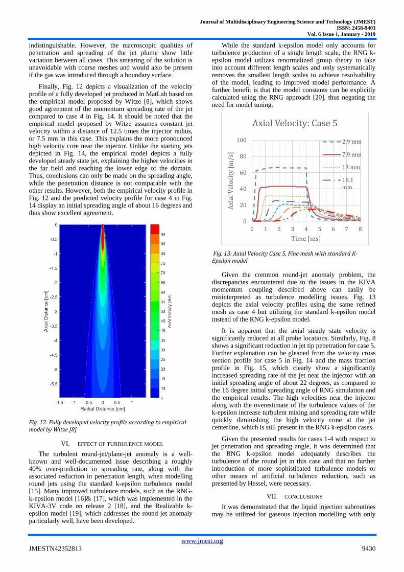
Fig. 13: Axial Velocity Case 5, Fine mesh with standard K-Epsilon model

Given the common round-jet anomaly problem, the discrepancies encountered due to the issues in the KIVA momentum coupling described above can easily be misinterpreted as turbulence modelling issues. Fig. 13 depicts the axial velocity profiles using the same refined mesh as case 4 but utilizing the standard k-epsilon model instead of the RNG k-epsilon model.

It is apparent that the axial steady state velocity is significantly reduced at all probe locations. Similarly, Fig. 8 shows a significant reduction in jet tip penetration for case 5. Further explanation can be gleaned from the velocity cross section profile for case 5 in Fig. 14 and the mass fraction profile in Fig. 15, which clearly show a significantly increased spreading rate of the jet near the injector with an initial spreading angle of about 22 degrees, as compared to the 16 degree initial spreading angle of RNG simulation and the empirical results. The high velocities near the injector along with the overestimate of the turbulence values of the k-epsilon increase turbulent mixing and spreading rate while quickly diminishing the high velocity cone at the jet centerline, which is still present in the RNG k-epsilon cases.

Given the presented results for cases 1-4 with respect to jet penetration and spreading angle, it was determined that the RNG k-epsilon model adequately describes the turbulence of the round jet in this case and that no further introduction of more sophisticated turbulence models or other means of artificial turbulence reduction, such as presented by Hessel, were necessary.

VII. CONCLUSIONS

It was demonstrated that the liquid injection subroutines may be utilized for gaseous injection modelling with only

0

20

40

60

80

100

0 1 2 3 4 5 6 7 8A

xial

Vel

oci

ty [

m/s

]

Time [ms]


2.9 mm

7.9 mm

13 mm

18.1mm



ISSN: 2458-9403


www.jmest.org

JMESTN42352813 9431

minor modifications, which leads to a fast implementation time.

It was shown that this methodology allows for the accurate simulation of round gaseous jets, as long as the mesh size near the injector and jet core is on the order of the injector radius, in order to capture the smallest feature of interest which in this case is the jet core velocity and mass distribution.

The macroscopic characteristics of the jet plume, including jet penetration and spreading angle, were reasonably well preserved far from the injector even as a coarser mesh size was used. A coarser mesh may be utilized if the near injector characteristics are not of great importance and no chemical reactions are modelled, such that mass fractions are of lower significance. Thus, in many cases a significant reduction in computational times may be achieved while maintaining adequate solution quality of the macroscopic jet plume characteristics.

As the mesh size becomes coarser, the high velocity and mass fraction gradient are lost due to smearing of the solution gradients. Especially for chemically reacting flows, the mass fraction gradient will have significant effects on the chemical reaction rates and thus a refined mesh near the injector on the order of the injector radius is necessary.

The injection methodology described in this paper does have some drawbacks. The algorithm will always center the injector location on the injection cell. This may lead to difficulties accurately positioning the injector within the mesh, especially with very coarse meshes. This may be remedied by refining the mesh at the injector location. Additionally, if multiple injectors/injector holes are modelled, each injector requires all 8 vertices of the injection cell without overlap to other injection cells in order to avoid cancellation of the momentum of opposing jets.

Modifications to distribute the parcel momentum to each vertex on the basis of the inverse distance-from-the-injector weighting instead of even distribution to all 8 vertices was deemed fundamentally unworkable in the context of the current KIVA code, as this introduces the invalid assumption of non-uniform subgrid mass distributions, which would require extensive modifications to KIVA.

It was found that upon the correction of the momentum coupling process, the RNG k-epsilon model described the jet characteristics well and adequately addressed the round jet anomaly. Thus, no additional modifications to the turbulence model were deemed necessary. This negates the necessity to introduce additional tuning constants to the model. Further, by immediate conversion of the parcels from the particle phase to the gas phase, and due to the relatively large size of the parcel volume compared to the cell volume, the mass fractions in the near injector area are well captured.

A significant flaw regarding the momentum coupling of the particle phase with the gas phase affecting both gaseous injection and evaporating liquid injection processes was discovered within KIVA. The simple modifications necessary to address this issue were outlined in detail. It is highly recommended that researchers utilizing KIVA or any KIVA derived codes verify that this issue does not pertain to their softwares and/or resolve it accordingly.

Ongoing efforts for further research are underway to extend this gaseous injection approach to function on a

pressure difference basis by modelling a constant pressure injector in order to improve its usability and applicability for internal combustion engine simulations, while taking into account compressibility effects.

REFERENCES

[1] G. Tryggvason, R. Scardovelli and S. Zaleski, "Direct Numerical

Simulations of Gas-Liquid Multiphase Flows," Cambridge University Press, 2011.

[2] J. Dukowicz, "A particle-fluid numerical model for liquid sprays," Journal of Computational Physics, vol. 35, no. 2, pp. 229-253, 1980.

[3] G. Micklow and W. Gong, "Investigation of the grid and Intake Generated Tumble on the In-Cylinder Flow of a Direct Injection Compression Ignition Engine," Journal of Automotive Engineering , vol. 222, no. 5, pp. 775-788, 2008.

[4] P. Ouellette, "Direct Injection of Natural Gas for Diesel Engine Fueling," Ph.D. Thesis, University of British Columbia, 1996.

[5] P. Ouellette and P. Hill, "Turbulent Transient Gas Injections," Journal of Fluids Engineering, vol. 122, p. 743, 2000.

[6] R. P. Hessel, N. Abani , S. M. Aceves and . D. L. Flowers, "Gaseous Fuel Injection Modeling Using a Gaseous Sphere Injection Methodology," in Powertrain & Fluid Systems Conference & Exhibition, Toronto, Canada, 2006.

[7] P. O. Witze, "Hot-Film Anemometer Measurements in a Starting Turbulent Jet," AIAA Journal, pp. 308-309, 1983.

[8] P. O. Witze, "The impulsively Started Incompressible Turbulent Jet," Sandia Laboratories Energy Report, pp. SAND80-8617, 1980.

[9] M. Choi, S. Lee and S. Park, "Numerical and experimental study of gaseous fuel injection for CNG direct injection," Fuel, vol. 140, pp. 693-700, 2015.

[10] N. Vargaftik, Tables on the Thermophysical Properties of Liquids and Gases, New York: Halsted Press, 1975.

[11] A. Amsden, P. O'Rourke and T. Butler, "KIVA-II: A Computer Program for Chemically Reactive Flows with Sprays," Los Alamos Report LA-11560-MS, 1989.

[12] N. Nordin, "Complex Chemistry Modeling of Diesel Spray Combustion," PhD Dissertation, Chalmers University of Technology, Gothenburg, Sweden, 2001.

[13] N. Abani and R. Reitz, "A Model to Predict Spray-tip Penetration for Time-varying Injection Profiles," in ILASS Americas, 20th Annual Conference on Liquid Atomization and Spray Systems, Chicago, IL, May 2007.

[14] N. Abani and R. Reitz, "Unsteady turbulent round jets and vortex motion," Physics of Fluids, vol. 19, no. 12, 2007.

[15] S. Pope, "An explanation of the turbulent round-jet/plane-jet anomaly," AIAA Journal, vol. 16, no. 3, pp. 279-282, 3 1978. Z. Han and D. Reitz, "Turbulence Modeling of Internal Combustion Engines Using RNG k-epsilon Models," Combustion Science and Technology, vol. 106, pp. 267-295, 1995.

[16] Z. Han and D. Reitz, "Turbulence Modeling of Internal Combustion Engines Using RNG k-epsilon Models," Combustion Science and Technology, vol. 106, pp. 267-295, 1995.



ISSN: 2458-9403


www.jmest.org

JMESTN42352813 9432

[17] S. Lam, "On the RNG theory of turbulence," Physics of Fluids A, vol. 4, no. 5, pp. 1007-1017, 1992.

[18] A. Amsden, "KIVA-3V: A Block-Structured KIVA Program for Engines with Vertical or Canted Valves," Los Alamos Report LA-13313-MS, 1997.

[19] T. Shih, A. Shabbir, Z. Yang and J. Zhu, "A New k-epsilon Eddy Viscosity Model for High Reynolds Number Turbulent Flows - Model Development and Validation," NASA Technical Memorandum, vol. 1994, 106721.

[20] V. Yakhot, S. Orszag, S. Thangam, T. Gatski and C. Speziale, "Development of turbulence models for shear flows by a double expansion technique," Physics of Fluids A, vol. 4, no. 7, pp. 1510-1520, 1992.

VIII. APPENDIX

Fig. 14: Velocity Profiles

Fig. 15: Mass Fraction Profiles


gaseous and liquid jet direct injection simulations using ... · regarding the particle momentum...

Documents