The views expressed here are the author’s and not necessarily those of the Federal Reserve Bank of Atlanta or the Federal Reserve System. Any remaining errors are the author’s responsibility. Please address questions regarding content to Patrick Higgins, Research Department, Federal Reserve Bank of Atlanta, 1000 Peachtree Street NE, Atlanta, GA 30309-4470, 404-498-7906, patrick.higgins@atl.frb.org. Federal Reserve Bank of Atlanta working papers, including revised versions, are available on the Atlanta Fed’s website at frbatlanta.org/pubs/WP/. Use the WebScriber Service at frbatlanta.org to receive e-mail notifications about new papers.

FEDERAL RESERVE BANK of ATLANTA WORKING PAPER SERIES

GDPNow: A Model for GDP “Nowcasting” Patrick Higgins Working Paper 2014-7 July 2014 Abstract: This paper documents GDPNow, a “nowcasting” model for gross domestic product (GDP) growth that synthesizes the “bridge equation” approach relating GDP subcomponents to monthly source data with the factor model approach used by Giannone, Reichlin, and Small (2008). The GDPNow model forecasts GDP growth by aggregating 13 subcomponents that make up GDP with the chain-weighting methodology used by the U.S. Bureau of Economic Analysis. Using current vintage data, out-of-sample GDPNow model forecasts are found to be more accurate than a number of statistical benchmarks since 2000. Using real-time data since the second-half of 2011, GDPNow model forecasts are found to be only slightly inferior to consensus near-term GDP forecasts from Blue Chip Economic Indicators. The forecast error variance of GDP growth for each of the GDPNow model, Blue Chip, and the Federal Reserve staff’s Green Book is decomposed as the sum of the forecast error covariances for the contributions to growth of the subcomponents of GDP. The decompositions show that “net exports” and “change in private inventories” are particularly difficult subcomponents to nowcast. JEL classification: E37, C53 Key words: nowcasting, forecasting, macroeconometric forecasting

“It is no longer true that academics are the people best informed about the evolution of next quarter’s GDP as was the case even in the 1960s.”

[Lawrence Summers, “Economic specialization is a feature, not a bug”1, July 26, 2011]

Section 1: Introduction

The view expressed by Lawrence Summers in the above quote is probably right. Perusing the June 2014 Wall Street Journal Economic Forecasting Survey2, one sees that most of the panelists submitting forecasts of GDP growth and other economic indicators are mostly business economists3. As documented by Landefeld, Seskin and Fraumeni (2008), survey-based data available to the public account for about 70 percent of the expenditure share of the “advance” (or first) estimate of gross domestic product (GDP) released 25 to 30 days after the end of a quarter. Both business economists and Federal Reserve staff economists utilize much of this available data when making very short-run GDP forecasts. As former Fed staff economists Jon Faust and Jonathan Wright put it in their 2009 paper evaluating the historical accuracy of Fed staff forecasts, “by mirroring key elements of the data construction machinery of the Bureau of Economic Analysis, the Fed staff forms a relatively precise estimate of what BEA will announce for the previous quarter’s GDP even before it is announced.” And yet, this “bottom-up” approach of mimicking of the BEA’s methods of translating publically available data into an estimate of GDP is less straightforward than it might seem. Much of recent literature on GDP “nowcasting” utilize fairly sophisticated econometric techniques in a “top-down” approach to directly forecast GDP without forecasting its subcomponents.

This paper describes a GDP “nowcasting” model called GDPNow that attempts to marry the econometrics used in the “top-down” approaches with the careful attention to the details of GDP data construction used in “bottom-up” approaches. After a brief summary of the GDP nowcasting literature in Section 2, we describe the GDPNow model in detail in Section 3. Section 4 evaluates the forecasting performance of the GDPNow model and Section 5 concludes. An appendix includes some technical details as well as tables documenting the data and sources used in the GDPNow model.

1 The article is available at http://blogs.reuters.com/lawrencesummers/2011/07/26/economic-specialization-is-a-feature-not-a-bug/ 2 Available at http://online.wsj.com/public/resources/documents/wsjecon0614.xls 3 There are a few exceptions, for example, Edward Leamer of UCLA Anderson School of Management.

Section 2: Literature Review

There is a large literature on “nowcasting” U.S. GDP growth; we briefly review and classify the studies according to their approach. For a good technical treatment of the methods of this literature, see Foroni and Marcellino (2013).

1.) Simple regression approaches: Braun (1990) uses two simple regression models, one relating quarterly production workers hours growth to quarterly GNP4 growth and a second using an Okun’s law equation with the unemployment rate and model-based estimates of the natural rate of unemployment and potential GNP. Ingenito and Trehan (1996) use a simple regression model of real GDP growth on a constant, three lags, and both nonfarm payroll employment growth and real consumption growth for the current quarter. Both Braun (1990) and Ingenito and Trehan (1996) address how they forecast the missing values of the monthly series needed for their models. Similar one-equation regression based forecast models of GDP growth are used by Fitzgerald and Miller (1989) and Koenig and Dolomas (1997).

2.) “Medium Data” or “Data-rich” Methods Without Component Forecasting: Kitchen and Kitchen (2013) run 24 simple univariate regressions of quarterly GDP growth on contemporaneous and lagged values of one other regressor. They combine the forecasts of these models using normalized R-squares from the regressions as weights. Carriero, Clark, and Marcellino (2012) consider a number of statistical models including various mixed frequency models which relate GDP growth to up to 9 monthly indicators and lags of GDP growth. The lags of the monthly indicators imply up to 50 explanatory variables in their model. To avoid overfitting, the authors use Bayesian methods. Giannone, Reichlin and Small (2008) use a dynamic factor model to nowcast GDP. Their model, which includes roughly 200 monthly macroeconomic indicators, can handle the “jagged edge” nature of staggered data releases so that the forecaster need not throw away data when predicting GDP growth. Finally, Schorfheide and Song (2013) develop an 11-variable mixed-frequency Bayesian vector autoregression (BVAR) that combines monthly and quarterly data by using state-space and Monte Carlo methods to estimate the posterior distribution of unobserved monthly values for real GDP [and other quarterly series]. Beauchemin (2014) adapted the Schorfheide and Song (2013) approach for the Minneapolis Mixed Frequency Vector Autoregression (MF-VAR) model. Forecasts from the MF-VAR model are regularly posted on the Minneapolis Fed’s website.

3.) Bridge Equation Methods/Tracking Models: This approach, pioneered by Nobel Laureate Lawrence R. Klein; is discussed in Klein and Sojo (1989). In short, one forecasts the major expenditure components of GDP using bridge equations that regress the growth rate of a component on one or more related monthly series5. Missing values of the monthly series in the quarter of interest are forecasted, generally by a univariate time series models like an ARIMA. The forecasts of the GDP components are then aggregated up to a GDP forecast using a national

4 Prior to 1992, GNP was most often used to measure aggregate output. 5 The monthly series are generally aggregated to a quarterly growth rate in the bridge equations.

income accounting identity. In today’s jargon, bridge equation type models are often called “tracking models”. There are a number of proprietary tracking forecasts currently in use such as the Current Quarter Model from Moody’s Analytics [see Zeller and Sweet (2012)] and GDP tracking forecasts from Macroeconomic Advisers6. Other bridge equation based approaches for nowcasting U.S. GDP growth include Payne (2000) and Miller and Chin (1996). We will borrow heavily from Miller and Chin (1996) and say more about their paper as we describe our approach.

Section 3: The GDPNow model

GDPNow borrows heavily from Miller and Chin (1996) and Giannone, Reichlin and Small (2008). Since the model builds up its GDP forecast from a forecast of subcomponents, it is a “tracking model” according to the above classification.

In short, the model uses the following six steps:

(1) Forecast the high-level subcomponents of GDP – 13 of them – with a quarterly BVAR only using data through the last quarter. This step is used by Chin and Miller (1996).

(2) Use a variant of the nowcasting model of Giannone, Reichlin and Small (2008) with a large number of data series to extract an underlying factor of economic activity akin to the Chicago Fed National Activity Index.

(3) Following Stock and Watson (2002), include this factor in factor augmented autoregressions to forecast a large number of monthly data series. For each series, aggregate the actual available data and the monthly forecasts into a quarterly percent (log) change.

(4) For each of the investment and government spending GDP components in step (1), run two sets of “bridge equation” regressions. The first set regresses a “granular” subcomponent of an expenditure component on one or more of the monthly series aggregated to the quarterly frequency in Step 3 [e.g. manufactured homes investment growth is regressed on a measure of real mobile home shipments growth]. The forecasts of the “granular” subcomponents are aggregated up to a forecast for the quarterly series. This forecast and the BVAR forecast from step (1) are included in a second bridge equation.

(5) Construct forecasts of consumption, imports/exports, and inventory investment using slightly different approaches.

6 Occasionally, these tracking forecasts have been available on the Macroeconomic Advisers blog http://macroadvisers.net/blog/. For a brief description of GDP tracking by Ben Herzon of Macroeconomic Advisers, see Herzon (2013).

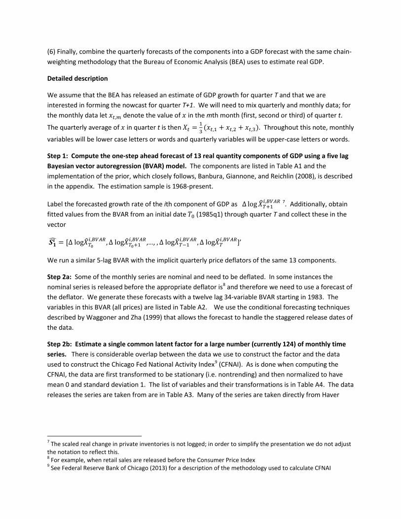
(6) Finally, combine the quarterly forecasts of the components into a GDP forecast with the same chain-weighting methodology that the Bureau of Economic Analysis (BEA) uses to estimate real GDP.

Detailed description

We assume that the BEA has released an estimate of GDP growth for quarter T and that we are interested in forming the nowcast for quarter T+1. We will need to mix quarterly and monthly data; for the monthly data let 𝑥𝑡,𝑚 denote the value of 𝑥 in the mth month (first, second or third) of quarter t.

The quarterly average of 𝑥 in quarter t is then 𝑋𝑡 = 13

(𝑥𝑡,1 + 𝑥𝑡,2 + 𝑥𝑡,3). Throughout this note, monthly

variables will be lower case letters or words and quarterly variables will be upper-case letters or words.

Step 1: Compute the one-step ahead forecast of 13 real quantity components of GDP using a five lag Bayesian vector autoregression (BVAR) model. The components are listed in Table A1 and the implementation of the prior, which closely follows, Banbura, Giannone, and Reichlin (2008), is described in the appendix. The estimation sample is 1968-present.

Label the forecasted growth rate of the ith component of GDP as ∆ log𝑋�𝑇+1𝑖,𝐵𝑉𝐴𝑅 7. Additionally, obtain

fitted values from the BVAR from an initial date 𝑇0 (1985q1) through quarter T and collect these in the vector

𝑺𝟏𝒊� = [∆ log𝑋�𝑇0𝑖,𝐵𝑉𝐴𝑅 ,∆ log𝑋�𝑇0+1

𝑖,𝐵𝑉𝐴𝑅,…, ,∆ log𝑋�𝑇−1𝑖,𝐵𝑉𝐴𝑅 ,∆ log𝑋�𝑇

𝑖,𝐵𝑉𝐴𝑅]’

We run a similar 5-lag BVAR with the implicit quarterly price deflators of the same 13 components.

Step 2a: Some of the monthly series are nominal and need to be deflated. In some instances the nominal series is released before the appropriate deflator is8 and therefore we need to use a forecast of the deflator. We generate these forecasts with a twelve lag 34-variable BVAR starting in 1983. The variables in this BVAR (all prices) are listed in Table A2. We use the conditional forecasting techniques described by Waggoner and Zha (1999) that allows the forecast to handle the staggered release dates of the data.

Step 2b: Estimate a single common latent factor for a large number (currently 124) of monthly time series. There is considerable overlap between the data we use to construct the factor and the data used to construct the Chicago Fed National Activity Index9 (CFNAI). As is done when computing the CFNAI, the data are first transformed to be stationary (i.e. nontrending) and then normalized to have mean 0 and standard deviation 1. The list of variables and their transformations is in Table A4. The data releases the series are taken from are in Table A3. Many of the series are taken directly from Haver

7 The scaled real change in private inventories is not logged; in order to simplify the presentation we do not adjust the notation to reflect this. 8 For example, when retail sales are released before the Consumer Price Index 9 See Federal Reserve Bank of Chicago (2013) for a description of the methodology used to calculate CFNAI

Analytics; these series generally have an “@” appearing in the series name. Other series need to be modified somehow; like being deflated by a price and/or spliced with another series10.

Denoting the ith pre-transformed series as 𝑦𝑡,ℎ𝑖 , and it’s post-transformed standardized value as 𝑧𝑡,ℎ

𝑖 , the estimated factor model is

(1) 𝑓𝑡,ℎ = 𝜌1𝑓𝑡,ℎ−1 + 𝜌2𝑓𝑡,ℎ−2 + 𝜌3𝑓𝑡,ℎ−3 + 𝑢𝑡,ℎ

(2) 𝑧𝑡,ℎ𝑖 = 𝛾1𝑖𝑓𝑡,ℎ + 𝜀𝑡,ℎ

𝑖

The latent factor is 𝑓𝑡,ℎ. To keep the notation of mixing monthly and quarterly data consistent throughout the note we adopt the notational convention that if 1 ≤ ℎ ≤ 3 , then

… = 𝑥𝑡−1,ℎ+3 = 𝑥𝑡,ℎ = 𝑥𝑡+1,ℎ−3 = ⋯

I.e., in our notation, the fourth month of quarter t-1 is also the first month of quarter t.

Doz, Giannone, and Reichlin (2006) show that the parameters and the variances of the error terms (𝑢𝑡,ℎ and 𝜀𝑡,ℎ

𝑖 ) in equations (1) and (2) can be consistently estimated by first estimating the latent factor(s) with simple principal components11 and then estimating both (1) and (2) with OLS. The latent factor(s) can then be extracted with the Kalman filter and Kalman smoother. In an extension of the Doz, Giannone, and Reichlin (2006) model; Giannone, Reichlin, and Small (2008) show how a dynamic factor model of this type can be extended to handle non synchronous data releases where some series are released in a more timely fashion than others. We follow the Giannone, Reichlin, and Small (2008) approach to generate an estimate of the time series of the smoothed factors. We also forecast future values of the factor using equation (1) and the last [smoothed] estimates of the factors. I.e. if month h-1 in quarter t is the last month where we have data on at least some of the series, then we have estimates of 𝑓𝑡,ℎ−1,𝑓𝑡,ℎ−2, and 𝑓𝑡,ℎ−3 but not 𝑓𝑡,ℎ. We then use (1) to forecast 𝑓𝑡,ℎ ,𝑓𝑡,ℎ+1, … . This follows the Giannone, Reichlin, and Small (2008)12 approach.

Step 3: Forecast the monthly series of interest using a variant of the Stock and Watson (2002) approach. Suppose we are interested in forecasting values for the values 𝑦𝑡,ℎ

𝑖 , 𝑦𝑡,ℎ+1𝑖 , … when we have

the non-missing observations … ,𝑦𝑡,ℎ−2𝑖 , 𝑦𝑡,ℎ−1

𝑖 . Similar to Stock and Watson (2002), we run factor augmented auotregressions of the form

10 E.g. the NAICS based manufacturing and trade sales series need to be spliced with SIC based counterparts, 11 Stock and Watson (2002) describe a method for estimating principal components when some series are missing at the beginning of the sample. In our application, an example of such a series is the ISM Nonmanufacturing Index which is only available starting July 1997. We implement Stock and Watson’s method in our application. 12 We do differ from Giannone, Reichlin, and Small (2008) in that we do not use month h data until we have the ISM Manufacturing Index for month h. This implies that series from the Reuters/University of Michigan and Conference Board consumer surveys as well as series from the Philly Fed Business Outlook Survey are not used until the ISM Manufacturing Index is released.

(3) ∆ log(𝑦𝑡,ℎ𝑖 ) = 𝛼𝑖 + �𝛾𝑘𝑖 ∆ log(𝑦𝑡,ℎ−𝑘

𝑖 )𝑞

𝑘=1

+ �𝛽𝑗𝑖𝑓𝑡,ℎ−𝑗

𝑟

𝑗=0

where the estimated factors 𝑓𝑡,ℎ from Step 2 are used. The number of lags of the dependent variable, q, and the number of lags of the factors, r, are selected with the Akaike Information Criterion (AIC) where we restrict 1 ≤ 𝑞 ≤ 12 and 0 ≤ 𝑟 ≤ 3. In the case of the consumption variables, we restrict 6 ≤ 𝑞 ≤12. Since we are able to forecast the factors as far out into the future as we’d like, we can recursively forecast ∆ log (𝑦𝑡,ℎ

𝑖 ), ∆ log (𝑦𝑡,ℎ+1𝑖 ), … as well. This approach is different from Stock and Watson (2002)

in the sense that they do not forecast future values of the factor and iteratively roll-over the one step ahead forecasts. Rather, they make h-step ahead projections directly with the available factors.

Step 4a: Run “bridge equation” regressions [investment and government spending components]. We explain this step for residential investment; the same method is also used for nonresidential structures investment, equipment investment, intellectual property products investment (IPP), federal government spending and state+local government spending.

The 13 GDP components used in our quarterly BVAR model are too coarse to be bridged directly with the monthly indicators in a manner that mimics the way BEA actually constructs GDP. For example, in the advance GDP estimate, monthly Census Bureau data on manufactured home shipments13 are the primary source for the manufactured homes subcomponent of real residential investment. This monthly series is not used for the other components of residential investment. Not surprisingly, the quarterly growth rate of manufactured home shipments has a much higher correlation with real manufactured home investment growth [r = 0.82, 1990Q1-2012Q4] than with total real residential investment growth [r = 0.41]. Rather than including very small components like manufactured home investment in the quarterly BVAR, and run the risk of over-fitting, we proceed as follows:

Partition nominal and real residential investment into 7 subcomponents

BEA Residential Investment Subcomponent

2012Q4 Share of Residential Investment

Monthly Indicator

Permanent-site 41.3% SplicedNewHousingConstruction Manufactured homes 0.9% MobileHomeVal Dormitories 0.8% NONE [Use AR(4)] Improvements 39.2% SplicedBuildingMaterials Brokers’ commissions on sale of structures

16.4% valExHomeSales+ valNewHomeSales

13 Available at http://www.census.gov/construction/mhs/mhsindex.html

Residential equipment

2.3% RetSalesResEquip

Net purchases of used structures

-0.9% NOT USED

The monthly indicators, which are price-deflated, are listed in Table A4. “Net purchases of used structures” is not used because it is negative and only available since 1995Q1

a.) For each of the monthly series, we use equation (3) to forecast the quarterly growth rate for the quarter of interest (T+1). For example, on the day before the quarter T+1 advance GDP release 𝑦𝑇+1,3MobileHomeVal will not be available, but 𝑦𝑇+1,2

MobileHomeVal will be. Therefore, we use (3) to obtain the forecast 𝑦�𝑇+1,3

MobileHomeVal and construct

(4) ∆ log (𝑌�𝑇+1MobileHomeVal) = log (𝑦𝑇+1,1MobileHomeVal + 𝑦𝑇+1,2

MobileHomeVal + 𝑦�𝑇+1,3MobileHomeVal

𝑦𝑇,1MobileHomeVal + 𝑦𝑇,2

MobileHomeVal + 𝑦𝑇,3MobileHomeVal )

The forecasted value ∆ log (𝑌�𝑇+1MobileHomeVal) will have less predictive power for manufactured home investment than the actual unavailable value ∆ log (𝑌𝑇+1MobileHomeVal) due to the missing value for the last month. Therefore, we also use (3) to construct the fitted values

(5) ∆ log (𝑌�𝑡MobileHomeVal) = log (𝑦𝑡,1MobileHomeVal + 𝑦𝑡,2

MobileHomeVal + 𝑦�𝑡,3MobileHomeVal

𝑦𝑡−1,1MobileHomeVal + 𝑦𝑡−1,2

MobileHomeVal + 𝑦𝑡−1,3MobileHomeVal )

for t <T+1. If we are making our nowcast well before the advance GDP release, (4) and (5) will also incorporate forecasts for 𝑦𝑡,2

MobileHomeVal and perhaps 𝑦𝑡,1MobileHomeVal. This is the same

method Chin and Miller (1996) use.

b.) For each subcomponent of real residential investment, 𝑅𝑒𝑎𝑙𝑅𝑒𝑠𝐼𝑛𝑣𝑡i, and its 𝑛𝑖 associated monthly indicator(s), we estimate the bridge equation regression

(6) ∆ log (𝑅𝐸𝐴𝐿𝑅𝐸𝑆𝐼𝑁𝑉𝑡i) = 𝜑𝑖 + �𝜃𝑘𝑖∆ log (𝑌�𝑡i)𝑛𝑖

𝑘=1

and make the forecast ∆ log (𝑅𝐸𝐴𝐿𝑅𝐸𝑆𝐼𝑁𝑉� 𝑇+1i ). The bridge equation is estimated with data

since 1985:Q1. For dormitories investment growth – and any other subcomponents for which we do not have a related monthly series – we use an AR(4) forecast.

c.) For the first six components of the above residential investment list, we compute the time T

spending shares 𝑆𝐻𝑇j = 𝑁𝑂𝑀𝑅𝐸𝑆𝐼𝑁𝑉𝑇

j

∑ 𝑁𝑂𝑀𝑅𝐸𝑆𝐼𝑁𝑉𝑇k6

𝑘=1 . The bridge model forecast of real residential

investment is

(7) ∆ log (𝑅𝐸𝐴𝐿𝑅𝐸𝑆𝐼𝑁𝑉�𝑇+1Bridge) = �𝑆𝐻𝑇i ∆ log (𝑅𝐸𝐴𝐿𝑅𝐸𝑆𝐼𝑁𝑉� 𝑇+1

i )6

𝑖=1

This weighting uses the fact that the growth rate of a Tornqvist index is a very good approximation of the growth rate of a Fisher index, even when time T expenditure weights are used instead of the average of the time T and time T+1 spending weights. Using the time t-1 spending shares 𝑆𝐻𝑡−1i , we go backwards in time to construct the fitted values

∆ log (𝑅𝐸𝐴𝐿𝑅𝐸𝑆𝐼𝑁𝑉�𝑡Bridge).

For the three major categories of nonresidential fixed investment [equipment, IPP and structures] and for both major categories of government spending [federal and state+local] we also use the same weighted average of bridge equations approach. The subcomponents and related monthly series used in the bridge equations are provided in Tables A5a, A5b, A5c, A5d, A5e and A5f.

Step 4b: Combine “bridge equation” forecasts with BVAR forecasts [investment and government spending components].

As Chin and Miller (1996) note, bridge models only use a subset of the data that go into the BEA’s estimate of GDP growth. Following the lead of these authors, we combine the bridge equation based forecast and the Step 1 BVAR forecast for six of the low-level GDP components. The regression combination equation for residential investment growth is

(8) ∆ log(𝑅𝐸𝐴𝐿𝑅𝐸𝑆𝐼𝑁𝑉𝑡)

= 𝛿𝑅𝑒𝑠𝐼𝑛𝑣∆ log�𝑅𝐸𝐴𝐿𝑅𝐸𝑆𝐼𝑁𝑉� 𝑡BVAR�+ (1 − 𝛿𝑅𝑒𝑠𝐼𝑛𝑣)∆ log �𝑅𝐸𝐴𝐿𝑅𝐸𝑆𝐼𝑁𝑉�

𝑡Bridge� + Ε𝑡

We estimate (8) with restricted least squares (RLS)14 and omit a constant from the regression since both of the right hand side terms in (8) are already forecasts of the left hand side term. As we get more

monthly housing data, ∆ log �𝑅𝐸𝐴𝐿𝑅𝐸𝑆𝐼𝑁𝑉�𝑡Bridge� will become more accurate on average and 𝛿𝑅𝑒𝑠𝐼𝑛𝑣

will get smaller. We use a similar approach for equipment, IPP, and nonresidential structures investment and for both federal and state+local government expenditures.

Step 5: Forecasting Real Net Exports. Forecasting net exports is tricky; Chin and Miller (1996), for example, forecast net exports as a residual by forecasting GDP directly15, forecasting all of the other components of GDP, and backing out net exports. As they note, the net exports forecasts from this method are not very accurate. Our approach for forecasting net exports of goods16 is the following:

14 We constrain 𝛿𝑅𝑒𝑠𝐼𝑛𝑣 to be between 0 and 1. 15 Chin and Miller (1996) using a simple regression of GDP growth on 1.) a constant, 2.) their quarterly BVAR prediction of GDP, 3.) quarterly real consumption growth using monthly data extrapolated with predictions from their monthly BVAR model, 4.) quarterly production hours growth using monthly data extrapolated with predictions from their monthly BVAR model. 16 An isomorphic approach is used for services.

a.) We construct monthly series on real goods imports and real goods exports using Census Bureau/BEA data on nominal goods imports/exports17 and monthly BLS data on imports and exports prices. The (NSA) exports price index for all commodities is taken directly from the U.S. Import and Export Price Indexes release18. Goods import price inflation is constructed as a weighted average of 8 import price inflation rates from the same release19. The petroleum import price index is manually seasonally adjusted [using the default Haver settings] while the other series are not. The weights are the categories’ nominal import shares from the prior quarter in NIPA table 4.2.5. The two-year lag in revision of the weights in the BLS import price index20 causes some discrepancy between the BLS import price series for all commodities and the BEA import price series for goods from NIPA table 4.2.4.

b.) We then construct an estimate of the contribution of goods net exports to real monthly GDP growth using the formula

(9) 𝑐𝑜𝑛𝑡𝑔𝑜𝑜𝑑𝑠𝑛𝑒𝑡𝑒𝑥𝑝𝑜𝑟𝑡𝑠𝑇+1,ℎ = 𝑛𝑜𝑚𝑔𝑜𝑜𝑑𝑠𝑒𝑥𝑝𝑜𝑟𝑡𝑠𝑇+1,ℎ−1𝑛𝑜𝑚𝑔𝑑𝑝𝑇+1,ℎ−1

∆ log (𝑟𝑒𝑎𝑙𝑔𝑜𝑜𝑑𝑠𝑒𝑥𝑝𝑇+1,ℎ)

−𝑛𝑜𝑚𝑔𝑜𝑜𝑑𝑠𝑖𝑚𝑝𝑜𝑟𝑡𝑠𝑇+1,ℎ−1𝑛𝑜𝑚𝑔𝑑𝑝𝑇+1,ℎ−1

∆ log (𝑟𝑒𝑎𝑙𝑔𝑜𝑜𝑑𝑠𝑖𝑚𝑝𝑇+1,ℎ)

Formula 9 is approximately the contribution to growth from a Tornqvist index; it is a very accurate approximation to the contribution to percent change used by the BEA. Monthly nominal GDP is a splice of the series constructed by Macroeconomic Advisers21 and Stock and Watson22.

c.) Next, we estimate a factor-augmented autoregression with 𝑐𝑜𝑛𝑡𝑔𝑜𝑜𝑑𝑠𝑛𝑒𝑡𝑒𝑥𝑝𝑜𝑟𝑡𝑠𝑇+1,ℎ exactly as we did in equation (3).

(10) 𝑐𝑜𝑛𝑡𝑔𝑜𝑜𝑑𝑠𝑛𝑒𝑡𝑒𝑥𝑝𝑜𝑟𝑡𝑠𝑡,ℎ = �𝛾𝑘𝑁𝑋𝑐𝑜𝑛𝑡𝑔𝑜𝑜𝑑𝑠𝑛𝑒𝑡𝑒𝑥𝑝𝑜𝑟𝑡𝑠𝑡,ℎ−𝑘

𝑞

𝑘=1

+�𝛽𝑗𝑁𝑋𝑓𝑡,ℎ−𝑗

𝑟

𝑗=0

Lag lengths are again selected using the AIC. We do not include a constant in the regression so that longer horizon forecasts of the net exports contribution converge to 0.

d.) We separately estimate factor augmented autoregressions for real goods exports growth and real goods imports growth [this time with a constant term included], and generate forecasts

17 The series are on a balance of payments basis and are available from Exhibit 1 of the FT-900 Census Bureau/BEA U.S. International Trade in Goods and Services release at http://www.census.gov/foreign-trade/Press-Release/current_press_release/ft900.pdf. 18 See http://www.bls.gov/news.release/ximpim.t02.htm. 19 See http://www.bls.gov/news.release/ximpim.t01.htm. 20 See http://www.bls.gov/news.release/ximpim.tn.htm. 21 See http://www.macroadvisers.com/content/MA_Monthly_GDP_Index.xlsx. Since the series is released with a longer lag than the international trade data; we forecast using a constant 4.5% (SAAR) monthly growth rate where necessary. 22 See http://www.princeton.edu/~mwatson/mgdp_gdi.html.

∆ log (𝑟𝑒𝑎𝑙𝑔𝑜𝑜𝑑𝑠𝑒𝑥𝑝𝑜𝑟𝑡𝑠� 𝑇+1,ℎ+1) and ∆ log (𝑟𝑒𝑎𝑙𝑔𝑜𝑜𝑑𝑠𝚤𝑚𝑝𝑜𝑟𝑡𝑠� 𝑇+1,ℎ+1) where h is the last month we have trade data for.

The forecasts ∆ log (𝑟𝑒𝑎𝑙𝑔𝑜𝑜𝑑𝑠𝑒𝑥𝑝𝑜𝑟𝑡𝑠� 𝑇+1,ℎ+1) and ∆ log (𝑟𝑒𝑎𝑙𝑔𝑜𝑜𝑑𝑠𝚤𝑚𝑝𝑜𝑟𝑡𝑠� 𝑇+1,ℎ+1) will not, in general, be consistent with 𝑐𝑜𝑛𝑡𝑔𝑜𝑜𝑑𝑠𝑛𝑒𝑡𝑒𝑥𝑝𝑜𝑟𝑡𝑠� 𝑇+1,ℎ+1; as (9) will not hold. Therefore we solve for

the unique adjustment factor 𝛼𝑇+1,ℎ+1𝑁𝑋𝑎𝑑𝑗 that imply the adjusted forecasts

∆log ( 𝑟𝑒𝑎𝑙𝑔𝑜𝑜𝑑𝑠𝑒𝑥𝑝�𝑇+1,ℎ+1𝑁𝑋𝑎𝑑𝑗 ) = ∆ log�𝑟𝑒𝑎𝑙𝑔𝑜𝑜𝑑𝑠𝑒𝑥𝑝� 𝑇+1,ℎ+1�+ 𝛼𝑇+1,ℎ+1

𝑁𝑋𝑎𝑑𝑗

and

∆log (𝑟𝑒𝑎𝑙𝑔𝑜𝑜𝑑𝑠𝚤𝑚𝑝�𝑇+1,ℎ+1𝑁𝑋𝑎𝑑𝑗 ) = ∆ log�𝑟𝑒𝑎𝑙𝑔𝑜𝑜𝑑𝑠𝚤𝑚𝑝� 𝑇+1,ℎ+1� − 𝛼𝑇+1,ℎ+1

𝑁𝑋𝑎𝑑𝑗

are mutually consistent with equations (9) and (10). We repeat the forecast/adjustment process through the 3rd month of quarter T+1. Then, if h = 1 for example, the monthly model forecast for the (approximate) contribution of goods net exports to GDP growth in quarter T+1 is:

(12) 𝐶𝑂𝑁𝑇𝐺𝑂𝑂𝐷𝑆𝑁𝐸𝑇𝐸𝑋𝑃𝑂𝑅𝑇𝑆�𝑇+1𝑀𝑜𝑛𝑡ℎ𝑙𝑦𝑀𝑜𝑑𝑒𝑙

=𝐵𝐸𝐴𝑁𝑂𝑀𝐺𝑂𝑂𝐷𝑆𝐸𝑋𝑃𝑂𝑅𝑇𝑆𝑇

𝑁𝑂𝑀𝐺𝐷𝑃𝑇log�

𝑟𝑒𝑎𝑙𝑔𝑜𝑜𝑑𝑠𝑒𝑥𝑝𝑇+1,1 + 𝑟𝑒𝑎𝑙𝑔𝑜𝑜𝑑𝑠𝑒𝑥𝑝�𝑇+1,2𝑁𝑋𝑎𝑑𝑗 + 𝑟𝑒𝑎𝑙𝑔𝑜𝑜𝑑𝑠𝑒𝑥𝑝�

𝑇+1,3𝑁𝑋𝑎𝑑𝑗

𝑟𝑒𝑎𝑙𝑔𝑜𝑜𝑑𝑠𝑒𝑥𝑝𝑇,1 + 𝑟𝑒𝑎𝑙𝑔𝑜𝑜𝑑𝑠𝑒𝑥𝑝𝑇,2 + 𝑟𝑒𝑎𝑙𝑔𝑜𝑜𝑑𝑠𝑒𝑥𝑝𝑇,3�

−𝐵𝐸𝐴𝑁𝑂𝑀𝐺𝑂𝑂𝐷𝑆𝐼𝑀𝑃𝑂𝑅𝑇𝑆𝑇

𝑁𝑂𝑀𝐺𝐷𝑃𝑇log�

𝑟𝑒𝑎𝑙𝑔𝑜𝑜𝑑𝑠𝑖𝑚𝑝𝑇+1,1 + 𝑟𝑒𝑎𝑙𝑔𝑜𝑜𝑑𝑠𝚤𝑚𝑝�𝑇+1,2𝑁𝑋𝑎𝑑𝑗 + 𝑟𝑒𝑎𝑙𝑔𝑜𝑜𝑑𝑠𝚤𝑚𝑝�

𝑇+1,3𝑁𝑋𝑎𝑑𝑗

𝑟𝑒𝑎𝑙𝑔𝑜𝑜𝑑𝑠𝑖𝑚𝑝𝑇,1 + 𝑟𝑒𝑎𝑙𝑔𝑜𝑜𝑑𝑠𝑖𝑚𝑝𝑇,2 + 𝑟𝑒𝑎𝑙𝑔𝑜𝑜𝑑𝑠𝑖𝑚𝑝𝑇,3�

Going backwards through time [and using in-sample forecasts for the same months where we don’t

have data], we generate the fitted values 𝐶𝑂𝑁𝑇𝐺𝑂𝑂𝐷𝑆𝑁𝐸𝑇𝐸𝑋𝑃𝑂𝑅𝑇𝑆� 𝑡𝑀𝑜𝑛𝑡ℎ𝑙𝑦𝑀𝑜𝑑𝑒𝑙 for t < T+123. We

generate alternative fitted values 𝐶𝑂𝑁𝑇𝐺𝑂𝑂𝐷𝑆𝑁𝐸𝑇𝐸𝑋𝑃𝑂𝑅𝑇𝑆� 𝑡𝐵𝑉𝐴𝑅 by using the BVAR growth

forecasts for real goods exports and real goods imports in place of the [log] growth rates in (12). We estimate the regression

(13) 𝐶𝑂𝑁𝑇𝐺𝑂𝑂𝐷𝑆𝑁𝐸𝑇𝐸𝑋𝑃𝑂𝑅𝑇𝑆𝑡= 𝛿𝑁𝑋𝐺𝑜𝑜𝑑𝑠𝐶𝑂𝑁𝑇𝐺𝑂𝑂𝐷𝑆𝑁𝐸𝑇𝐸𝑋𝑃𝑂𝑅𝑇𝑆� 𝑡

𝐵𝑉𝐴𝑅

+ (1 − 𝛿𝑁𝑋𝐺𝑜𝑜𝑑𝑠)𝐶𝑂𝑁𝑇𝐺𝑂𝑂𝐷𝑆𝑁𝐸𝑇𝐸𝑋𝑃𝑂𝑅𝑇𝑆� 𝑡𝑀𝑜𝑛𝑡ℎ𝑙𝑦𝑀𝑜𝑑𝑒𝑙 + Ε𝑡

by RLS where 𝐶𝑂𝑁𝑇𝐺𝑂𝑂𝐷𝑆𝑁𝐸𝑇𝐸𝑋𝑃𝑂𝑅𝑇𝑆𝑡 is the share-weighted growth rate of real goods exports less the share-weighted growth rate of real goods imports [using time t-1 expenditure shares]. The final forecast of real goods exports (imports) growth is a weighted average of the BVAR [weight 𝛿𝑁𝑋𝐺𝑜𝑜𝑑𝑠] and “monthly data model” [weight 1 − 𝛿𝑁𝑋𝐺𝑜𝑜𝑑𝑠] forecasts.

23 We are assuming we have one month of international trade in quarter T+1 and have to use forecasts for the last two months. Obviously, if the amount of available monthly data was different, then a different number of “hats”.

The forecasts for imports and exports in services are generated using exactly the same approach24.

Step 6: Forecast consumption directly. Since PCE consumption spending is already monthly, there is no need to use bridge equations. For the monthly consumption components that we use to partition total consumption, we still forecast the months that are not available with equation (3). The subcomponents of PCE consumption that we use are listed in Table A6. As described by Chapter 5 of the NIPA Handbook: Concepts and Methods of the U.S. National Income and Product Accounts, the BEA uses the “retail control” method to estimate consumption for many durable and nondurable goods25. For these goods, whenever retail sales from the U.S. Census Bureau is released (around the middle of the month), we use the latest growth rate in nominal sales for the “retail control” group – Retail Sales & Food Services Excluding Auto, Gas Stations & Building Materials –as a forecast of the growth rate in nominal consumption for the analogous PCE bundle26. We also assume that revisions in retail control sales will result in a proportional revision to the retail control basket in the PCE. The Consumer Price Index is also released around the middle of the month. Price measures for the PCE retail control subcomponents can (almost exactly) be mapped into CPI subcomponents. Whenever the Consumer Price Index is released we use the appropriate components to “nowcast” the inflation rate for the PCE retail control basket. Table A7 contains the mapping we use from CPI to PCE components.

The BEA does not use retail sales to estimate PCE new motor vehicle sales, but they do publish unit light-weight auto and truck sales about a week before retail sales are released27. The BEA also publishes data on the consumer share of auto and light truck sales28. We use all of this data to nowcast the real PCE new motor vehicle sales for the latest month whenever the BEA’s unit vehicle sales data is released. For the other PCE components we do not exploit other monthly releases to predict the latest month’s numbers, although one could certainly do so. As shown in Table A6, we partition goods into 4 subcomponents and services into 2 subcomponents. Assuming, for example, we have h=2 months of PCE data in quarter T+1, our forecast for real PCE goods consumption growth in quarter T+1 is

(14) ∆ log (𝑅𝐸𝐴𝐿𝑃𝐶𝐸� 𝑇+1Goods)

= �{�𝑁𝑂𝑀𝐺𝑂𝑂𝐷𝑆𝑇𝑘

∑ 𝑁𝑂𝑀𝐺𝑂𝑂𝐷𝑆𝑇𝑗4

𝑗=1� 𝑙𝑜𝑔 �

𝑟𝑒𝑎𝑙𝑔𝑜𝑜𝑑𝑠𝑇+1,1𝑘 + 𝑟𝑒𝑎𝑙𝑔𝑜𝑜𝑑𝑠𝑇+1,2

𝑘 + 𝑟𝑒𝑎𝑙𝑔𝑜𝑜𝑑𝑠� 𝑇+1,3𝑘

𝑟𝑒𝑎𝑙𝑔𝑜𝑜𝑑𝑠𝑇,1𝑘 + 𝑟𝑒𝑎𝑙𝑔𝑜𝑜𝑑𝑠𝑇,2

𝑘 + 𝑟𝑒𝑎𝑙𝑔𝑜𝑜𝑑𝑠𝑇,3𝑘 �

4

𝑘=1

}

Notice that quarter T expenditure shares are used as weights in the forecast. Similarly, our forecast for real PCE services growth is

24 The monthly series for real service exports and imports are “SplicedServiceExports” and “SplicedServiceImports” shown in Table 4A. 25 See http://www.bea.gov/national/pdf/chapter5.pdf 26 Actually, we partition the retail control group into food services and non-food services and separately forecast their PCE analogs using the same technique. This allows us to construct separate “goods” and “services” forecasts of consumption growth. 27 See table 6 of http://www.bea.gov/national/xls/gap_hist.xls

28 See ASCPU@USNA and BusShareTrucks in Table A4. Since these series are released with a longer lag than unit auto sales, the latest months data on light auto/truck sales must be combined with the factor model forecasts of these variables.

(15) ∆ log (𝑅𝐸𝐴𝐿𝑃𝐶𝐸� 𝑇+1Svcs)

= �{�𝑁𝑂𝑀𝑆𝑉𝐶𝑆𝑇𝑘

∑ 𝑁𝑂𝑀𝑆𝑉𝐶𝑆𝑇𝑗2

𝑗=1� 𝑙𝑜𝑔 �

𝑟𝑒𝑎𝑙𝑠𝑣𝑐𝑠𝑇+1,1𝑘 + 𝑟𝑒𝑎𝑙𝑠𝑣𝑐𝑠𝑇+1,2

𝑘 + 𝑟𝑒𝑎𝑙𝑠𝑣𝑐𝑠� 𝑇+1,3𝑘

𝑟𝑒𝑎𝑙𝑠𝑣𝑐𝑠𝑇,1𝑘 + 𝑟𝑒𝑎𝑙𝑠𝑣𝑐𝑠𝑇,2

𝑘 + 𝑟𝑒𝑎𝑙𝑠𝑣𝑐𝑠𝑇,3𝑘 �

2

𝑘=1

}

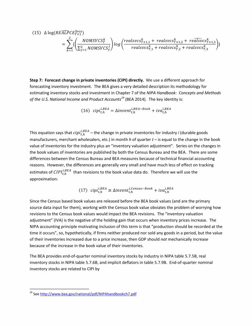
Step 7: Forecast change in private inventories (CIPI) directly. We use a different approach for forecasting inventory investment. The BEA gives a very detailed description its methodology for estimating inventory stocks and investment in Chapter 7 of the NIPA Handbook: Concepts and Methods of the U.S. National Income and Product Accounts29 (BEA 2014). The key identity is:

(16) 𝑐𝑖𝑝𝑖𝑡,ℎ𝑖,𝐵𝐸𝐴 = ∆𝑖𝑛𝑣𝑒𝑛𝑡𝑡,ℎ

𝑖,𝐵𝐸𝐴−𝐵𝑜𝑜𝑘 + 𝑖𝑣𝑎𝑡,ℎ𝑖,𝐵𝐸𝐴

This equation says that 𝑐𝑖𝑝𝑖𝑡,ℎ𝑖,𝐵𝐸𝐴 – the change in private inventories for industry i (durable goods

manufacturers, merchant wholesalers, etc.) in month h of quarter t – is equal to the change in the book value of inventories for the industry plus an “inventory valuation adjustment”. Series on the changes in the book values of inventories are published by both the Census Bureau and the BEA. There are some differences between the Census Bureau and BEA measures because of technical financial accounting reasons. However, the differences are generally very small and have much less of effect on tracking estimates of 𝐶𝐼𝑃𝐼𝑡,ℎ

𝑖,𝐵𝐸𝐴 than revisions to the book value data do. Therefore we will use the approximation:

(17) 𝑐𝑖𝑝𝑖𝑡,ℎ𝑖,𝐵𝐸𝐴 ≅ ∆𝑖𝑛𝑣𝑒𝑛𝑡𝑡,ℎ

𝑖,𝐶𝑒𝑛𝑠𝑢𝑠−𝐵𝑜𝑜𝑘 + 𝑖𝑣𝑎𝑡,ℎ𝑖,𝐵𝐸𝐴

Since the Census based book values are released before the BEA book values (and are the primary source data input for them), working with the Census book value obviates the problem of worrying how revisions to the Census book values would impact the BEA revisions. The “inventory valuation adjustment” (IVA) is the negative of the holding gain that occurs when inventory prices increase. The NIPA accounting principle motivating inclusion of this term is that “production should be recorded at the time it occurs”, so, hypothetically, if firms neither produced nor sold any goods in a period, but the value of their inventories increased due to a price increase, then GDP should not mechanically increase because of the increase in the book value of their inventories.

The BEA provides end-of-quarter nominal inventory stocks by industry in NIPA table 5.7.5B, real inventory stocks in NIPA table 5.7.6B, and implicit deflators in table 5.7.9B. End-of-quarter nominal inventory stocks are related to CIPI by

29 See http://www.bea.gov/national/pdf/NIPAhandbookch7.pdf

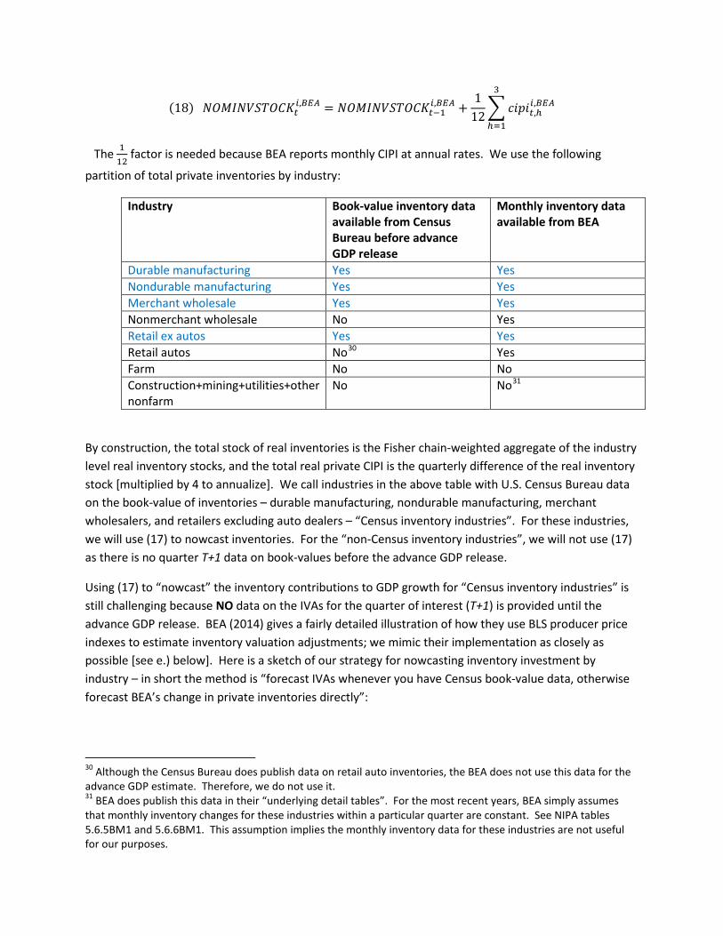
(18) 𝑁𝑂𝑀𝐼𝑁𝑉𝑆𝑇𝑂𝐶𝐾𝑡𝑖,𝐵𝐸𝐴 = 𝑁𝑂𝑀𝐼𝑁𝑉𝑆𝑇𝑂𝐶𝐾𝑡−1

𝑖,𝐵𝐸𝐴 +1

12�𝑐𝑖𝑝𝑖𝑡,ℎ

𝑖,𝐵𝐸𝐴3

ℎ=1

The 112

factor is needed because BEA reports monthly CIPI at annual rates. We use the following

partition of total private inventories by industry:

Industry Book-value inventory data available from Census Bureau before advance GDP release

Monthly inventory data available from BEA

Durable manufacturing Yes Yes Nondurable manufacturing Yes Yes Merchant wholesale Yes Yes Nonmerchant wholesale No Yes Retail ex autos Yes Yes Retail autos No30 Yes Farm No No Construction+mining+utilities+other nonfarm

No No31

By construction, the total stock of real inventories is the Fisher chain-weighted aggregate of the industry level real inventory stocks, and the total real private CIPI is the quarterly difference of the real inventory stock [multiplied by 4 to annualize]. We call industries in the above table with U.S. Census Bureau data on the book-value of inventories – durable manufacturing, nondurable manufacturing, merchant wholesalers, and retailers excluding auto dealers – “Census inventory industries”. For these industries, we will use (17) to nowcast inventories. For the “non-Census inventory industries”, we will not use (17) as there is no quarter T+1 data on book-values before the advance GDP release.

Using (17) to “nowcast” the inventory contributions to GDP growth for “Census inventory industries” is still challenging because NO data on the IVAs for the quarter of interest (T+1) is provided until the advance GDP release. BEA (2014) gives a fairly detailed illustration of how they use BLS producer price indexes to estimate inventory valuation adjustments; we mimic their implementation as closely as possible [see e.) below]. Here is a sketch of our strategy for nowcasting inventory investment by industry – in short the method is “forecast IVAs whenever you have Census book-value data, otherwise forecast BEA’s change in private inventories directly”:

30 Although the Census Bureau does publish data on retail auto inventories, the BEA does not use this data for the advance GDP estimate. Therefore, we do not use it. 31 BEA does publish this data in their “underlying detail tables”. For the most recent years, BEA simply assumes that monthly inventory changes for these industries within a particular quarter are constant. See NIPA tables 5.6.5BM1 and 5.6.6BM1. This assumption implies the monthly inventory data for these industries are not useful for our purposes.

a.) First estimate a monthly price BVAR and forecast, using Waggoner and Zha (1999) for months where some, but not all, of the data is available. Some of the forecasted prices will be used to deflate nominal values of sales or shipments in the BVAR estimated in step b.). Also, some of the forecasted prices are used in step e.) of the IVA derivation. We use the actual and forecasted values of monthly sales prices for the “Census inventory industries” to construct end-of-quarter T+1 forecasts for the inventory implicit price deflators for these industries32.

b.) Estimate a “core quantity” BVAR using 16 monthly series. The series, listed in Table A8a, include industry level data on employment, real sales and industrial production. The BVAR also includes the ISM composite manufacturing index and the inventories subcomponent of the index. The BVAR does not include any other inventory variables. The sales variables are deflated by one of the price variables used in a.); combining the real and price forecasts provides a forecast for nominal sales.

c.) Estimate 6 different “block” BVARs using a subset of variables from step b.) in the first block and one other industry inventory variable in the second block. The variables in the first block of each BVAR are also given in Table A8b. For the “Census inventory industries”, the inventory variable is the sum of the two terms on right hand side of (17) [Census change in book-value plus BEA IVA] divided [or scaled] by nominal industry level sales lagged by 6-months. For nonmerchant wholesaler and retail automotive inventories, the scaled inventory variable is in Table A8b. By construction, contemporaneous and lagged values in the first block can impact values in the second block while values in the second block cannot effect values in the first [either lagged or contemporaneously]. The dynamics of the variables in the first block are determined using the variables and parameter estimates in the step b.) BVAR. For example, the ISM Manufacturing Index appears in only the durable and nondurable manufacturing inventory blocks. The block structuring ensures that 1.) The ISM Manufacturing Index forecasts [coming from b.)] are the same in both manufacturing block BVARs 2.) The ISM Manufacturing Index values and forecasts directly affect the durable/nondurable manufacturing inventory forecasts but not the other inventory forecasts. The choice of variables for the block BVARs is motivated by the fact that inventory investment has a fairly high correlation with the difference between IP growth and real goods final sales growth. As in step a.), we use the conditional forecasting technique described by Waggoner and Zha (1999) to constrain the forecasts to equal the actual data wherever it is available. We are able to combine the “core quantity” BVAR and all of the block BVARs into one large BVAR by putting 0s in the appropriate places for both the lag coefficient parameters and the error covariance matrix.

d.) For the “Census inventory industries”, we use the nominal sales growth forecasts from a.) and b.), and the inventory forecasts [scaled by nominal sales] in c.) to back out a forecast for CIPI on the left hand side of (17). Wherever we have actual Census data on the book value of inventories, we can also use (17) to back out the implied IVA forecast that is consistent with both the CIPI forecast and the book value data. The log likelihood of a particular forecast for

32 The quarterly inventory implicit price deflators are taken from NIPA table 5.7.9B. The forecasts are derived from the monthly sales price series using a Denton interpolation procedure which interpolates a lower frequency variable with a related higher frequency one.

quarters T and T+1 data, conditional on monthly data through the end of quarter T-1 [for which there will be no missing data] and the BVAR parameter estimates, is straightforward to calculate33.

e.) Whenever we get Census book-value data on inventories in “Census inventory industry” i, we also use an alternative forecasting model of the IVA using the aforementioned BEA (2014) method of constructing IVAs with BLS PPI prices. The method requires combining “finished+work-in-progress” PPI goods prices with intermediate materials PPI prices. The raw sources we use for both types of prices are in Table A8c. The combined PPI prices need to be converted to “end-of-month prices” and then to “average monthly prices”; again see BEA (2014). All inventories are assumed to be “First in First Out” (FIFO) and the “turnover pattern” – the proportion of inventory stocks that sit on the shelves for exactly x-months34 – that best fits the data35 is used. The model implied IVAs do not exactly match the actual IVAs, and the autocorrelation of the “discrepancy errors” is positive. Therefore, we fit an AR(1) to these “discrepancy errors”. For any given pattern of industry i IVAs beyond the last available month36, and up until a terminal date for the PPI data [the 3rd month of quarter T+1 padding with forecasts of the PPIs where necessary from a.)], we can calculate the likelihood of a forecasted path of IVAs using the AR(1) model and a standard likelihood formula for an AR(1)37.

f.) We then use the log-likelihoods in the IVA/PPI models in e.) and the log-likelihood in the big BVAR in step d.) to estimate the values of the IVAs [for the months where we have Census book-values on inventories ] that maximize the sum of the likelihoods. This maximization step assumes that the error terms from d.) are independent from the error terms from e.). 38

g.) Once we have the most likely IVAs – for the months where we have Census book-values on inventories – we use (17) to back out the implied monthly CIPIs. We then use the large BVAR and the conditional forecasting algorithm from Waggoner and Zha (1999), to get forecasts of the CIPIs for industry-month pairs where we do not have Census book value data on inventories. This means we do not have to worry about forecasting IVAs for the months that we do not have Census book value data. The nominal CIPI forecasts and the forecasts of the associated price deflators are used to back out forecasts of the real inventory stocks. We use the same BVAR to get forecasts of CIPIs for retail auto dealer inventories and non-merchant wholesaler inventories, where no Census book value data is available.

33 See, for example Chapter 11 of Hamilton (1994), page 293 11.1.10. If Ω is the covariance matrix of the errors, and 𝒆𝑡 are the forecasted residuals in the BVAR, then the conditional log-likelihood we are referring to is logL�𝒚𝑇,1, … ,𝒚𝑇,6�Ω� ∝ − 1

2∑ 𝒆′𝑇,ℎΩ−16ℎ=1 𝒆𝑇,ℎ.

34 We assume x ≤ 5. 35 In terms of minimizing the scaled sum of squared differences between the BEA’s reported IVA and the model implied IVA. The scaling factor, which is “average monthly prices”, is used so that recent IVAs do not get much larger weights than older IVAs [due to inflation]. The “turnover pattern” weights are restricted to be nonnegative and sum to 1.0. 36 This will always be the 3rd month of quarter T. 37 See Hamilton 1994 (pages 118-119) for this likelihood. 38 It also assumes that the error terms from one IVA/PPI model, e.g. durable manufacturing, are independent from the error terms of a different IVA/PPI model, e.g. merchant wholesalers.

h.) For “farm” inventories and “construction+mining+utilities+other nonfarm” inventories, where no monthly data is available, we use an AR(4) with the quarterly series to generate forecasts for end of quarter T+139.

i.) We aggregate the forecasts of the [real] inventory stocks and their associated price deflators into the total real private inventory stock at the end of quarter T+1 using the same Fisher chain-weighting of inventory stocks that BEA (2014) uses.

Finally, we generate in-sample forecasts of the real change in private inventories for quarters T, T-1, T-2, … 1983q2, 1983q1 by repeating steps a.) – i.) and maintaining the same BVAR and IVA model parameter estimates. Before the “final” [3rd] estimate of GDP growth in quarter T, we replace the BEA’s “change in private inventories” with the estimate from the model. We do this because the model can account for revisions to Census data on the book-value of inventories that the BEA has not yet incorporated into their latest GDP estimate for quarter T.

We call the change in private inventories from the monthly model 𝐶𝐼𝑃𝐼�𝑡𝑀𝑜𝑛𝑡ℎ𝑙𝑦𝐷𝑎𝑡𝑎𝑀𝑜𝑑𝑒𝑙. The

quarterly BVAR in Step 1 gives us the alternative forecast 𝐶𝐼𝑃𝐼�𝑡𝑄𝑡𝑟𝑙𝑦𝐵𝑉𝐴𝑅. We combine these forecasts

by solving for the value of 𝛿𝑄𝑡𝑟𝑙𝑦𝐵𝑉𝐴𝑅 in (19) that minimizes the in-sample sum of squared differences between the predicted contribution of inventories to real GDP growth and the actual contribution of inventories to real GDP.

(19) 𝐶𝐼𝑃𝐼�𝑡𝐶𝑜𝑚𝑏𝑖𝑛𝑒𝑑𝑀𝑜𝑑𝑒𝑙 = (1 − 𝛿𝑄𝑡𝑟𝑙𝑦𝐵𝑉𝐴𝑅)𝐶𝐼𝑃𝐼�𝑡

𝑀𝑜𝑛𝑡ℎ𝑙𝑦𝐷𝑎𝑡𝑎𝑀𝑜𝑑𝑒𝑙 + 𝛿𝑄𝑡𝑟𝑙𝑦𝐵𝑉𝐴𝑅𝐶𝐼𝑃𝐼�𝑡𝑄𝑡𝑟𝑙𝑦𝐵𝑉𝐴𝑅

The formula for the contribution to percent change is provided in the appendix; for the non-inventory components we use the actual price and quantity components rather than the forecasted values.

Step 8: Calculate real GDP growth with a Fisher chain weighting formula the price and quantity indexes forecasted in the previous steps.

See the appendix. In this step, one has to be careful to enter both goods and services imports into the formula with a minus sign. Also, the implicit price deflator for inventories is end-of-quarter. To convert this price index to a quarterly average, the average of the current end-of-quarter and previous end-of-quarter prices is used.

Section 4: Horse Races:

Before we assess the forecasting performance of our model, we make a digression on the quality of the consensus (average) forecast from Blue Chip Economic Indicators. We are interested in answering the question “Which components of GDP are most responsible for forecast errors of GDP growth?”. Blue Chip Economic Indicators includes forecasts of the following GDP components: 1.) Real PCE

39 We use a 12-quarter moving average as the forecasts of the implicit price deflators.

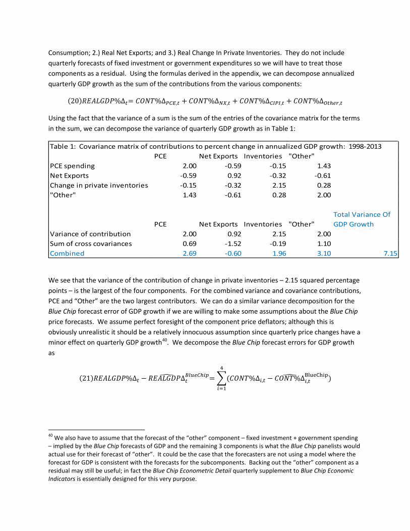
Consumption; 2.) Real Net Exports; and 3.) Real Change In Private Inventories. They do not include quarterly forecasts of fixed investment or government expenditures so we will have to treat those components as a residual. Using the formulas derived in the appendix, we can decompose annualized quarterly GDP growth as the sum of the contributions from the various components:

(20)𝑅𝐸𝐴𝐿𝐺𝐷𝑃%∆𝑡= 𝐶𝑂𝑁𝑇%∆𝑃𝐶𝐸,𝑡 + 𝐶𝑂𝑁𝑇%∆𝑁𝑋,𝑡 + 𝐶𝑂𝑁𝑇%∆𝐶𝐼𝑃𝐼,𝑡 + 𝐶𝑂𝑁𝑇%∆𝑂𝑡ℎ𝑒𝑟,𝑡

Using the fact that the variance of a sum is the sum of the entries of the covariance matrix for the terms in the sum, we can decompose the variance of quarterly GDP growth as in Table 1:

Table 1: Covariance matrix of contributions to percent change in annualized GDP growth: 1998-2013PCE Net Exports Inventories "Other"

PCE spending 2.00 -0.59 -0.15 1.43Net Exports -0.59 0.92 -0.32 -0.61Change in private inventories -0.15 -0.32 2.15 0.28"Other" 1.43 -0.61 0.28 2.00

PCE Net Exports Inventories "Other"Total Variance Of GDP Growth

Variance of contribution 2.00 0.92 2.15 2.00Sum of cross covariances 0.69 -1.52 -0.19 1.10Combined 2.69 -0.60 1.96 3.10 7.15

We see that the variance of the contribution of change in private inventories – 2.15 squared percentage points – is the largest of the four components. For the combined variance and covariance contributions, PCE and “Other” are the two largest contributors. We can do a similar variance decomposition for the Blue Chip forecast error of GDP growth if we are willing to make some assumptions about the Blue Chip price forecasts. We assume perfect foresight of the component price deflators; although this is obviously unrealistic it should be a relatively innocuous assumption since quarterly price changes have a minor effect on quarterly GDP growth40. We decompose the Blue Chip forecast errors for GDP growth as

(21)𝑅𝐸𝐴𝐿𝐺𝐷𝑃%∆𝑡 − 𝑅𝐸𝐴𝐿𝐺𝐷𝑃∆� 𝑡𝐵𝑙𝑢𝑒𝐶ℎ𝑖𝑝= �(𝐶𝑂𝑁𝑇%∆𝑖,𝑡 − 𝐶𝑂𝑁𝑇%Δ�

𝑖,𝑡BlueChip)

4

𝑖=1

40 We also have to assume that the forecast of the “other” component – fixed investment + government spending – implied by the Blue Chip forecasts of GDP and the remaining 3 components is what the Blue Chip panelists would actual use for their forecast of “other”. It could be the case that the forecasters are not using a model where the forecast for GDP is consistent with the forecasts for the subcomponents. Backing out the “other” component as a residual may still be useful; in fact the Blue Chip Econometric Detail quarterly supplement to Blue Chip Economic Indicators is essentially designed for this very purpose.

We use the final Blue Chip forecast made about three weeks before the advance GDP release41. These forecasts are made after the “first final” GDP estimates for the previous quarter, so we don’t have to worry about revisions to the previous quarter’s net exports or CIPI estimates. The actual GDP growth rate and contributions in (21) use real-time data from the “advance” GDP release. We do not include advance GDP releases that are part of a benchmark or comprehensive revision to the NIPA since we don’t know how much of the revisions to net exports and CIPI the Blue Chip forecasters are anticipating. If we square both sides of (21) and average the N forecasts across time we can decompose the average squared Blue Chip forecast error of GDP growth as42:

(22)1𝑁

� (𝑅𝐸𝐴𝐿𝐺𝐷𝑃%∆𝑡 − 𝑅𝐸𝐴𝐿𝐺𝐷𝑃∆� 𝑡𝐵𝑙𝑢𝑒𝐶ℎ𝑖𝑝)2

2014𝑄1

𝑡=1998𝑄1

= �{1𝑁

� (𝐶𝑂𝑁𝑇%∆𝑖,𝑡 − 𝐶𝑂𝑁𝑇%Δ�𝑖,𝑡BlueChip)2

2014𝑄1

𝑡=1998𝑄1

}4

𝑖=1

+ �{1𝑁

� �[(𝐶𝑂𝑁𝑇%∆𝑖,𝑡 − 𝐶𝑂𝑁𝑇%Δ�𝑖,𝑡BlueChip)(𝐶𝑂𝑁𝑇%∆𝑗,𝑡

𝑗≠𝑖

2014𝑄1

𝑡=1998𝑄1

4

𝑖=1

− 𝐶𝑂𝑁𝑇%Δ�𝑗,𝑡BlueChip)]}

We call each of the first four summands in curly braces on the right hand side of (22) “the average squared forecast error of component i’s contribution to GDP growth” and the last four summands in curly braces “the average sum of cross products for contribution i”. Table 2 has both of these terms for each of the four subcomponents of GDP; it also has the full 4x4 cross product matrix of the average product of the forecast errors43.

41 Also, we construct the contributions to percentage change – both for the Blue Chip forecasts and for the actuals – using the chain-weighting formulas described in the appendix. This insures that if the component forecasts were all exactly right then the forecasted contributions would match the actual contributions. This wouldn’t be the case if we used the BEA’s published contributions to percent changes for several technical reasons [e.g. the BEA contributions are calculated using 1000+ components]. 42 Since there are 15 benchmark/comprehensive revision quarters for GDP over the 1998Q1-2014Q1 period, N=46. To simplify notation, we do not adjust the 𝑡 = 1998𝑄1to 2014𝑄1 notation in (22). 43 The (i,j) entry in this matrix is 1

𝑁∑ (𝐶𝑂𝑁𝑇%∆𝑖,𝑡 − 𝑅𝐸𝐴𝐿𝐺𝐷𝑃∆�

𝑖,𝑡𝐵𝑙𝑢𝑒𝐶ℎ𝑖𝑝2012𝑄4

𝑡=1998𝑄1 ) (𝐶𝑂𝑁𝑇%∆𝑗,𝑡 − 𝐶𝑂𝑁𝑇∆�𝑗,𝑡𝐵𝑙𝑢𝑒𝐶ℎ𝑖𝑝)

PCE Net Exports CIPI "Other"PCE spending 0.40 -0.04 -0.14 -0.02Net Exports -0.04 0.72 -0.27 -0.16Change in private inventories -0.14 -0.27 0.78 -0.24"Other" -0.02 -0.16 -0.24 1.05

PCE Net Exports CIPI "Other"

MSE Of GDP growth forecast

Average squared forecast error of the contribution to GDP growth 0.40 0.72 0.78 1.05 2.94Sum of cross products -0.21 -0.48 -0.66 -0.43 -1.77Combined 0.19 0.24 0.12 0.62 1.17

RMSE 1.08

Table 2: Product matrix of average Blue Chip forecast errors for contributions to growth: 1998q1-2014q1

In Table 2, we see that the PCE contribution forecasts are more accurate than the other three components. This is perhaps not surprising since most of the consumption data for the quarter is directly available to the forecasters. However, for both net exports and CIPI, the cross-interactions of the forecast error with the other forecast errors cancel out much of their contribution to the total mean squared forecast error. Laurence Meyer, of Macroeconomic Advisers, noted this cancellation of forecast errors for GDP components in a speech he made while he was a Federal Reserve Governor:

My colleague at Washington University, Murray Weidenbaum, has suggested that forecast errors are often offsetting, reflecting the work of a saint who watches over forecasters. Her name is St. Offset. Her work is often observed when a forecaster gets a forecast for GDP in a particular quarter almost perfect, but misses by a wide amount on nearly every component of GDP!44

It appears that “St. Offset” is indeed assisting the Blue Chip panelists. It also appears that the “other” component is responsible for much of their GDP forecast error. One should perhaps not read too much into this as “other” could also be picking up the unobserved discrepancy between the panelists GDP forecasts and their forecasts of the components.

As an alternative, we repeat the same exercise with the last Greenbook45 “nowcast” of the contributions to real GDP growth. One advantage of the Greenbook “nowcasts” is that they contain a much more

44 Speech available at http://www.federalreserve.gov/boarddocs/speeches/1998/19980108.htm. This reference was originally cited by Payne (2000). 45 The Federal Reserve’s Bluebook and Greenbook were combined into one document now called the Tealbook.

detailed component breakdown of GDP. They also contain the contributions themselves. The sum of the forecasted contributions equals GDP forecast apart from a negligible rounding error46. A disadvantage with using the Greenbook forecasts is that they are released with a lag of 5 to 6 years.

We use “advance release” BEA published contributions to change – available since the advance 1999Q3 release – since there is no need to construct the Greenbook contributions. The production date of the last Greenbook was anywhere from 1 day to 44 days before the advance GDP release over the 1999Q3-2008Q3 period. On average it was published 24 days before the release47. Table 3 contains the same component breakdown as the Blue Chip survey48:

PCENet Exports CIPI "Other"

PCE spending 0.24 0.00 -0.06 0.08Net Exports 0.00 0.24 -0.11 -0.08Change in private inventories -0.06 -0.11 0.32 -0.04"Other" 0.08 -0.08 -0.04 0.26

PCENet Exports CIPI "Other"

MSE Of GDP growth forecasts

Average squared forecast error of the contribution to GDP growth 0.24 0.24 0.32 0.26 1.06Average sum of cross products 0.02 -0.19 -0.21 -0.05 -0.43Combined 0.26 0.05 0.11 0.22 0.64

RMSE 0.80

Table 3: Product matrix of average Greenbook forecast errors for contributions to real GDP growth: 1999Q3-2008Q3

Again, “St. Offset” is reducing the impact of the forecast errors of net exports and CIPI. This is also apparent for a more conventional breakdown of the GDP components shown in Table 4:

46 The Greenbook forecasts are rounded to the nearest tenth of a percentage point. 47 The last Blue Chip survey is generally taken a little over 3 weeks before the advance GDP release. 48 “Other” is calculated as the residual between the GDP nowcast and the sum of the other 3 contributions.

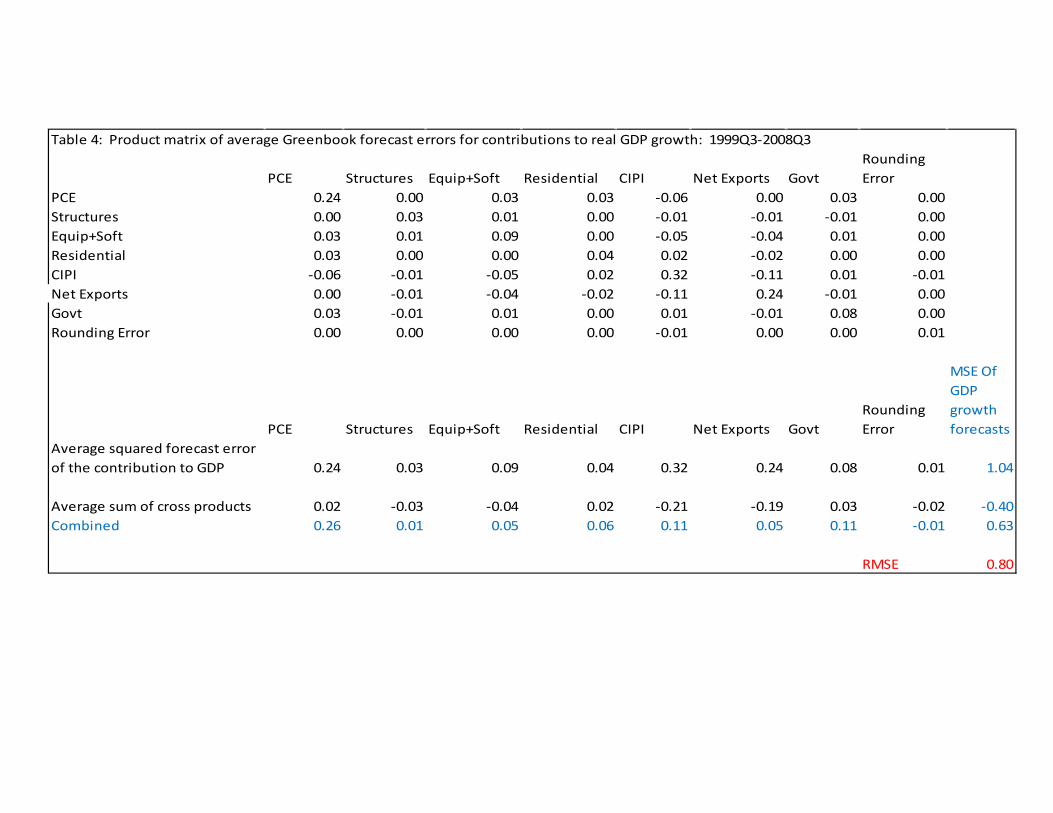
PCE Structures Equip+Soft Residential CIPI Net Exports GovtRounding Error

PCE 0.24 0.00 0.03 0.03 -0.06 0.00 0.03 0.00Structures 0.00 0.03 0.01 0.00 -0.01 -0.01 -0.01 0.00Equip+Soft 0.03 0.01 0.09 0.00 -0.05 -0.04 0.01 0.00Residential 0.03 0.00 0.00 0.04 0.02 -0.02 0.00 0.00CIPI -0.06 -0.01 -0.05 0.02 0.32 -0.11 0.01 -0.01Net Exports 0.00 -0.01 -0.04 -0.02 -0.11 0.24 -0.01 0.00Govt 0.03 -0.01 0.01 0.00 0.01 -0.01 0.08 0.00Rounding Error 0.00 0.00 0.00 0.00 -0.01 0.00 0.00 0.01

PCE Structures Equip+Soft Residential CIPI Net Exports GovtRounding Error

MSE Of GDP growth forecasts

Average squared forecast error of the contribution to GDP 0.24 0.03 0.09 0.04 0.32 0.24 0.08 0.01 1.04

Average sum of cross products 0.02 -0.03 -0.04 0.02 -0.21 -0.19 0.03 -0.02 -0.40Combined 0.26 0.01 0.05 0.06 0.11 0.05 0.11 -0.01 0.63

RMSE 0.80

Table 4: Product matrix of average Greenbook forecast errors for contributions to real GDP growth: 1999Q3-2008Q3

We now turn to the horse races. Unfortunately, due to the data intensive nature of the GDPNow model49, it is not feasible to use real-time data for a long sample. Therefore we conduct what Stock and Watson (2007) call a “pseudo-out-of-sample” forecasting exercising. We implement this as follows:

Algorithm for evaluating root mean square forecast error (RMSFE)

1.) Take a snapshot of all of the data on the day before the advance 2014:Q1 GDP release (April 30, 2014).

2.) For each of the monthly data series, toss out the last h observations of the series that were available through April 29, 2014 [where h is divisible by 3]. For each of the quarterly series, toss out the last h/3 available observations available through April 29, 2014. Use the truncated dataset to estimate the model and forecast GDP growth [for the April 29, 2014 vintage of data] for the quarter that was h/3 quarters before 2014:Q1. This is essentially the forecasting exercise that Giannone, Reichlin, and Small (2008) use50.

Repeating step 2.) for h = 3, 6, … , 165, 168 generates out of sample forecasts for 2000:Q1 – 2013:Q4. Some of the alternative benchmark models “cheat” to give them an advantage over the GDPNow model. The models are:

1.) Rolling-window AR(2): The model is

(22)Δlog (𝑅𝑒𝑎𝑙𝐺𝐷𝑃𝑡) = 𝛼0 + 𝛼1Δlog (𝑅𝑒𝑎𝑙𝐺𝐷𝑃𝑡−1) + 𝛼2Δlog (𝑅𝑒𝑎𝑙𝐺𝐷𝑃𝑡−2) + 𝑢𝑡 At each time t0, (22) is estimated with OLS by using the last h* observations of Δlog (𝑅𝑒𝑎𝑙𝐺𝐷𝑃𝑡) through t0 [Δlog (𝑅𝑒𝑎𝑙𝐺𝐷𝑃𝑡0−h∗+1),Δlog (𝑅𝑒𝑎𝑙𝐺𝐷𝑃𝑡0−h∗+2), … ,Δlog (𝑅𝑒𝑎𝑙𝐺𝐷𝑃𝑡0)] and the forecast for Δlog (𝑅𝑒𝑎𝑙𝐺𝐷𝑃𝑡0+1) is made. h* = 108 quarters is chosen to minimize the out-of-sample root mean square forecast error (RMSFE) for 2000:Q1 – 2013:Q4. Obviously, a forecaster would not know h* a priori. The rolling AR(2) performed slightly better than the AR(1) or AR(4).

2.) Rolling-window factor augmented AR(2): Let 𝑓𝑡,𝑚𝐶𝐹𝑁𝐴𝐼 denote the Chicago Fed National Activity

Index (CFNAI) in month m of quarter t. Since 𝑓𝑡,𝑚𝐶𝐹𝑁𝐴𝐼 is analogous to a 1-month (log) growth

rate, we relate it to quarterly GDP growth using the following moving average:

(23)𝐹𝑡𝐶𝐹𝑁𝐴𝐼 =19

[𝑓𝑡,3𝐶𝐹𝑁𝐴𝐼 + 2𝑓𝑡,2

𝐶𝐹𝑁𝐴𝐼 + 3𝑓𝑡,1𝐶𝐹𝑁𝐴𝐼 + 2𝑓𝑡−1,3

𝐶𝐹𝑁𝐴𝐼 + 𝑓𝑡−1,2𝐶𝐹𝑁𝐴𝐼]

49 We use well over 200 different time series. 50 Like these authors, we are using what they call a “stylized calendar” where one pretends that the timing of the data releases is always the same. Of course, the staggering of the data releases does in fact change slightly from quarter to quarter. Like these authors, we are ignoring this in our exercise.

Equation (23) approximately transforms the CFNAI into a quarterly growth rate; Koenig (2002) uses this same weighted average of the ISM manufacturing index to nowcast GDP growth. The forecasting equation is: (24)Δlog (𝑅𝑒𝑎𝑙𝐺𝐷𝑃𝑡)

= 𝛼0 + 𝛼1Δlog (𝑅𝑒𝑎𝑙𝐺𝐷𝑃𝑡−1)+𝛼2Δlog (𝑅𝑒𝑎𝑙𝐺𝐷𝑃𝑡−2) + 𝛼3𝐹𝑡𝐶𝐹𝑁𝐴𝐼 + 𝛼4𝐹𝑡−1𝐶𝐹𝑁𝐴𝐼

+ 𝑢𝑡 As before, rolling-window regressions of length h*quarters are used to forecast GDP growth, where h*=68 quarters is chosen to minimize the RMSFE. The model “cheats” by not choosing h* a priori. It also “cheats” because the forecaster would not see 𝑓𝑡,3

𝐶𝐹𝑁𝐴𝐼 in real-time51 and because the CFNAI is estimated using the entire data set. Alternative lag-lengths of the CFNAI and GDP growth had slightly higher RMSFEs.

3.) Mixed Frequency BVAR: This model, adapted from Schorfheide and Song (2013), is described in the appendix. We use a 7-lag monthly BVAR with the following 7 variables: real consumption, nonfarm payroll employment, industrial production, the ISM Manufacturing Index, housing starts growth multiplied by residential investment’s share of GDP, real capital goods shipments, and real GDP. As in Schorfheide and Song (2013), real GDP is a latent monthly variable estimated by the Kalman smoother. Rather than use the Monte Carlo Markov Chain (MCMC) algorithm developed by Schorfheide and Song (2013), we use the Expectation-maximization (EM) algorithm. In quarter t, we assume that we have all 3 months of data for the non-latent variables except real PCE. For real PCE, we need to forecast data for the third month of quarter t as that data point would not be available until after the “advance” GDP release.

4.) Quarterly BVAR: We use the same 5-lag quarterly BVAR with the quantity components of GDP that we used in step 1 as well as the same 5-lag quarterly BVAR with the implicit deflators. The growth forecasted is then computed using the chain-weighting formula A3 in the appendix.

5.) Tracking model – monthly series only: In the GDPNow model, each of the non-consumption component forecasts is a weighted average of the monthly indicator based forecast and the quarterly BVAR forecast. Here we set the weight on the BVAR forecasts to 0.

6.) Full tracking model (GDPNow): This is the Atlanta Fed GDPNow model.

51 This is not entirely accurate because 𝑓𝑡,3𝐶𝐹𝑁𝐴𝐼 is released before the advance estimate of 𝑅𝑒𝑎𝑙𝐺𝐷𝑃𝑡. However,

about a third of the monthly series used to compute 𝑓𝑡,3𝐶𝐹𝑁𝐴𝐼 are missing at the time of the release, so projected

values are used in their place. See Federal Reserve Bank of Chicago (2013).

In Table 5 below, RMSFEs are calculated using annualized percent changes, not log-differences52, since users are typically interested in the former. The Diebold-Mariano (1995) test statistics use the log-difference based forecast errors.

Table 5: Out of sample forecast performance on day before advance GDP release: 2000Q1 - 2013Q4

RMSFE

Diebold Mariano Test Statistic For Forecasts Compared To Model 5.) p-value

1.) Rolling AR(2)* 2.43 2.59 0.0095 2.) Rolling Factor Augmented AR(2)* 1.95 3.45 0.0006 3.) Mixed Frequency BVAR* 1.73 3.40 0.0007 4.) Quarterly BVAR* 2.28 2.65 0.0079 5.) Tracking model: Monthly version 1.22 0.68 0.4952 6.) GDPNow model 1.15

*Accuracy of forecast is different from Model 6.) at 1% signficance level

We see that the full tracking model – GDPNow – has the lowest RMSFE and is significantly better than the first four models at the 1% significance level. Since the last 3 model forecasts are built up from component level forecasts, we can trace the source of the forecast errors in Tables 6a – 6c as we did with the Blue Chip and Greenbook forecasts:

52 I.e we compute the mean-squared error of 100(exp (Δlog (𝑅𝑒𝑎𝑙𝐺𝐷𝑃𝑡))4 − exp (Δlog (𝑅𝑒𝑎𝑙𝐺𝐷𝑃𝑡))4� ).

PCE Equipment IPP Structures Residential Govt CIPI Net ExportsMSE Of GDP forecasts

Average squared forecast error of the contribution to GDP growth 1.26 0.36 0.03 0.13 0.24 0.39 1.05 0.86 4.31Average sum of cross products 0.38 0.52 0.12 0.04 0.17 -0.22 -0.10 -0.01 0.89Combined 1.63 0.88 0.15 0.16 0.41 0.17 0.95 0.85 5.20RMSFE of contribution 1.12 0.60 0.16 0.36 0.49 0.62 1.02 0.93

RMSFE 2.28

Table 6a: Decomposition of MSFE of GDP forecast of Quarterly BVAR from forecast errors of component contributions to GDP growth: 2000-2013

PCE Equipment IPP Structures Residential Govt CIPI Net ExportsMSE Of GDP forecasts

Average squared forecast error of the contribution to GDP growth 0.06 0.09 0.03 0.03 0.01 0.22 0.59 0.28 1.32Average sum of cross products 0.00 0.00 -0.02 0.01 0.04 0.11 0.05 -0.04 0.16Combined 0.06 0.09 0.01 0.04 0.05 0.33 0.65 0.25 1.48RMSFE of contribution 0.25 0.29 0.17 0.16 0.12 0.47 0.77 0.53

RMSFE 1.22

Table 6b: Decomposition of MSFE of GDP forecast of Monthly Model from forecast errors of component contributions to GDP growth: 2000-2013

PCE Equipment IPP Structures Residential Govt CIPI Net ExportsMSE Of GDP forecasts

Average squared forecast error of the contribution to GDP growth 0.06 0.12 0.03 0.03 0.01 0.23 0.51 0.30 1.28Average sum of cross products -0.01 0.00 0.00 0.01 0.04 0.07 0.02 -0.08 0.03Combined 0.05 0.11 0.02 0.03 0.06 0.30 0.53 0.21 1.32RMSFE of contribution 0.25 0.34 0.16 0.16 0.12 0.48 0.71 0.55

RMSFE 1.15

Table 6c: Decomposition of MSFE of GDP forecast of GDPNow Model from forecast errors of component contributions to GDP growth: 2000-2013

We see that the RMSFEs from Tables 6a – 6c do in fact match the RMSFEs from Table 5. The other conclusions we make from Tables 6a – 6c are:

1.) The tracking model forecasts of the components are superior to the quarterly BVAR forecasts for all of the components except “Intellectual Property Products” investment (IPP).

2.) Most of the improvement from the monthly data only tracking model to the full GDPNow model comes from the change in private inventories component.

3.) Comparing Table 6c.) and Table 4.), we see that the tracking model forecasts of CIPI and government spending are inferior to the Greenbook forecasts of these components [in spite of the tracking model’s informational advantage].

4.) Unfortunately, “St. Offset” does not help the tracking model forecasts as much as it does with the Greenbook and Blue Chip forecasts.

Conclusion 3.) is perhaps not surprising given the framework of our model in which one component of GDP is forecasted somewhat independently from another. As we saw in Table 1, when net exports has a below average contribution to GDP growth, this tends to be more than offset by positive contributions in the other components. A more unified modeling approach would perhaps be able to better capture the relationships between the components. For example, past Greenbooks have cited the Federal Reserve Board staff’s “flow-of-goods” system used to keep track of inventory movements53. We leave these improvements to the model to further research.

Finally, we test if our tracking model’s forecast accuracy improves as we get closer to the advance GDP release date. We do this by replacing April 29, 2014 in the “Algorithm for testing RMSFE” with the date that was k days before the 2014:Q1 release (on April 30, 2014). We take a snapshot of the data on this date and repeat the steps of the algorithm. Since 2014:Q1 growth was revised several times in the second quarter of 2014, we restrict the out-of-sample period to 2000:Q1 – 2013:Q4. The evolution of the RMSFE for 40 different snapshot dates is shown in the picture below.

53 See, e.g., http://www.federalreserve.gov/monetarypolicy/files/FOMC20071031gbpt220071024.pdf

Interestingly, the nowcasts stop improving about four weeks before the advance GDP release. This forecast exercise does not use real time data, and it may be the case that the short-run nowcasts improve as they incorporate data revisions. Even 85 days before the advance GDP release, the forecasts are slightly more accurate than the BVAR and AR(2) forecasts shown in Table 5.

We have been regularly updating our GDPNow model since the second half of 2011 thereby establishing a short track record which we reproduce in Table 7 below.

Table 7: Real-time forecasting performance of GDPNow Model

Quarter being forecasted

BEA's Advance Estimate (SAAR)

GDPNow Forecast Right Before BEA's Advance Estimate

Blue Chip Consensus Forecast 3 weeks before BEA's advance estimate

2011q3 2.5 3.2 1.92011q4 2.8 5.2 3.12012q1 2.2 3.0 2.22012q2 1.5 0.2 1.82012q3 2.0 1.8 1.72012q4 -0.1 0.1 1.42013q1 2.5 2.9 2.92013q2 1.7 1.3 1.72013q3 2.8 2.2 2.02013q4 3.2 3.1 2.42014q1 0.1 0.3 1.7

Average absolute error 0.68 0.62

Root-mean squared error 0.94 0.81

We see that over its short history, the GDPNow model has been slightly less accurate than the consensus forecast from Blue Chip Economic Indicators in spite of its informational advantage. Improvements have been made in the GDPNow model over time54 and, since 2011, the GDPNow forecasts have been slightly more accurate than the Blue Chip consensus. We certainly don’t want to read too much into this (yet!).

Section 5: Conclusions and extensions

It will be difficult to compare the GDPNow model ‘s performance to “professional” or “expert” forecasts until we establish a longer track record with real-time data. Nevertheless, it is probably safe to say that the GDPNow model forecasts are not as accurate as the best judgmental forecasts. The GDPNow model can still be useful since as it can be updated after virtually every major macroeconomic data release. Apart from improving the forecast performance of the GDPNow model, there are a number of possible extensions of this work. One would be cataloging with real-time data which releases are responsible for the largest increases in forecast accuracy. Giannone, Reichlin and Small (2008) found that the Business Outlook Survey release from the Federal Reserve Bank of Philadelphia led to a larger predictive improvement than many of the other releases. Since data from this survey are not used to

54 The GDPNow forecasts in Table 7 were made in real-time. Subsequent improvements to the model have not been used to rerun past forecasts using updated versions of the model with real-time vintages of the data.

construct GDP, the Philly Fed Survey may be less important for our model. A second extension would be to exploit higher frequency – weekly or daily – data. For instance, Andreou, Ghysles and Kourtellos (2013) used mixed data sampling (MIDAS) regressions to nowcast GDP growth with daily financial data. This approach might be particularly useful around business cycle turning points. A third extension would be to adapt the model to backcast revisions to GDP growth. Following certain key data releases of GDP source data, business economists often make projections of how they expect the BEA to revise the most recent GDP estimate in lieu of the new information. However, the academic literature has not addressed this topic using a “bottom-up” approach. The topic could be particularly relevant for Federal Reserve policymakers who make projections of fourth quarter over fourth quarter real GDP growth rates that, for the current year, are impacted by BEA revisions. A fourth extension would be incorporating the model’s forecasts into a DSGE model. Del Negro and Schorfheide (2012) provide evidence that conditioning Smets-Wouters (2007) DSGE forecasts on external Blue Chip Economic Indicators forecasts improves the short-run DSGE forecasts. Since Blue Chip Economic Indicators does not include a quarterly forecast for investment55, it would be interesting to see if incorporating it further improved the DSGE forecasts. Finally, the model could be extended to “nowcast” the GDP Deflator or other price deflators like the PCE price index. The Federal Reserve Bank of Cleveland has done recent work on this topic that they’ve made available to the public on their “Inflation Nowcasting” webpage56.

55 Many DSGE models exclude consumer durables from consumption, such as the Federal Reserve Bank of Philadelphia’s PRISM model: http://www.phil.frb.org/research-and-data/real-time-center/PRISM/ It would be fairly straightforward to decompose goods as “durables” and “nondurables” inside our model. 56 Knotek II and Zaman (2014) have developed their own model for nowcasting inflation that performs as well or better than expert forecasters. Daily updates of the model are available at http://www.clevelandfed.org/research/data/us-inflation/nowcasting/.

References:

Andreou, Elena , Eric Ghysels and Andros Kourtellos (2013) “Should Macroeconomic Forecasters Use Daily Financial Data and How?” Journal of Business & Economic Statistics, Vol. 31, No. 2, pp. 240-251.

Banbura, Marta, Giannone, Domenico and Lucrezia Reichlin (2008) “Large Bayesian VARs” European Central Bank Working Paper, No. 966 (November 2008).

Barhoumi, Karim, Véronique Brunhes-Lesage, Olivier Darné, Laurent Ferrara, Bertrand Pluyaud and Béatrice Rouvreau (2008) “Monthly Forecasting of French GDP: A Revised Version of the Optim Model” Banque of France Working Paper , No. 222 (September 2008).

Beauchemin, Kenneth (2014) “A 14-Variable Mixed-Frequency VAR Model” Federal Reserve Bank of Minneapolis Research Department Staff Report 493 December 2013

Braun, Steven (1990) “Estimation of Current-Quarter Gross National Product by Pooling Preliminary Labor-Market Data” Journal of Business and Economic Statistics, (July 1990). Vol. 8, No. 2, pp. 293-304.

Bureau of Economic Analysis (2014) “Concepts and Methods of the U.S. National Income and Product Accounts (Chapters 1-10 and 13)” (February 2014) Available at http://www.bea.gov/national/pdf/allchapters.pdf

Carriero, Andrea, Clark, Todd E., and Massimiliano Marcellino (2012) “Real-Time Nowcasting with a Bayesian Mixed Frequency Model with Stochastic Volatility” Federal Reserve Bank of Cleveland Working Paper No. 12-27.

Census Bureau (2013) “Construction Methodology” Available at http://www.census.gov/construction/c30/methodology.html

Chin, Daniel M. and Preston J. Miller (1996) “Using Monthly Data to Improve Quarterly Model Forecasts” Federal Reserve Bank of Minneapolis Quarterly Review, Vol. 20, No. 2, Spring 1996, pp. 16-33.

Del Negro, Marco and Frank Schorfheide (2013) “DSGE Model-Based Forecasting” in Graham Elliott and Allan Timmermann (eds.): "Handbook of Economic Forecasting," Vol 2A, 2013, Handbooks in Economics, Elsevier / North-Holland, pp. 57-140.

Diebold, Francis X. and Roberto S. Mariano (1995) “Comparing Predictive Accuracy” Journal of Business and Economic Statistics, July 1995, Vol. 13, No. 3.

Doz, Catherine, Giannone, Domenico and Lucrezia Reichlin (2006) "A Quasi Maximum Likelihood Approach For Large Approximate Dynamic Factor Models" European Central Bank Working Paper, No. 674 (September 2006).

Faust, Jon and Jonathan H. Wright (2009) “Comparing Greenbook and Reduced Form Forecasts Using a Large Realtime Dataset”, Journal of Business & Economic Statistics, Vol. 27, No. 4, pp. 468-479.

Federal Reserve Bank of Chicago (2013) “Background on the Chicago Fed National Activity Index” Available at http://www.chicagofed.org/digital_assets/publications/cfnai/background/cfnai_background.pdf

Fitzgerald, Terry J. and Preston J. Miller (1989) "A Simple Way to Estimate Current-Quarter GNP" Federal Reserve Bank of Minneapolis Quarterly Review, Fall, pp. 27-31.

Foroni, Claudia and Massimiliano Marcellino (2013) “A Survey of Econometric Methods for Mixed Frequency Data” Norges Bank Working Paper No. 2013-06.

Giannone, Domenico, Reichlin, Lucrezia and David Small (2008) “Nowcasting: The Real-Time Informational Content of Macroeconomic Data” Journal of Monetary Economics, No. 55 (2008) pp. 665-676.

Hamilton, James D. (1994) Time Series Analysis Princeton University Press.

Herzon, Ben (2013) “Using High-Frequency Data to Estimate GDP Growth in the Current Quarter” July 29-30 presentation at the 2013 NABE Economic Measurement Seminar, available at https://nabe.m3ams.com/Document/Download/16270026

Kitchen, Jackson and John Kitchen (2013) “Real-Time Forecasting Revisited: Letting the Data Decide” Business Economics, Vol. 48, pp. 8-28.

Klein, L.R. and E. Sojo (1989) “Combinations of High and Low Frequency Data in Macroeconometric Models” In Klein and Marquez (eds), Economics in Theory and Practice: An Eclectic Approach. Dordrecht: Kluwer, pp. 3-16.

Knotek II, Edward S. and Saeed Zaman (2014) “Nowcasting U.S. Headline and Core Inflation” Federal Reserve Bank of Cleveland Working Paper, No. 14-03.

Koenig, Evan F. and Shelia Dolomas (1997) “Real-Time GDP Growth Forecasts” Federal Reserve Bank of Dallas Working Paper, No. 97-10.

Koenig, Evan F. (2002) “Using the Purchasing Managers’ Index to Assess the Economy’s Strength and the Likely Direction of Monetary Policy” Federal Reserve Bank of Dallas Economic and Financial Policy Review, Vol. 1, No. 6

Landefeld. J. Steven, Seskin, Eugene P. and Barbara M. Fraumeni (2008) “Taking the Pulse of the Economy: Measuring GDP” Journal of Economic Perspective, Vol. 22, No. 2, Spring 2008, pp. 193–216.

Liu, Yanjun, Hamalainen, Nell and Bing-Sun Wong (2003) “Economic Analysis and Modelling Using Fisher Chain Data” Canada Department of Finance Working Paper, No. 2003-13.

Macroeconomic Advisers (2008) “Macroeconomic Advisers’ Measure of Monthly GDP” Macroeconomic Advisers’ Macro Focus, Vol. 3, No. 3, February 29, 2008.

Payne David R. (1999) “Predicting the Producers’ Durable Equipment Component of GDP – Gross Domestic Product” Business Economics, January 1999.

Payne David R. (2000) “Predicting GDP Growth Before the BEA’s Advance GDP Release: A How-To Manual” Business Economics, January 1999.

Schorfheide, Frank and Dongho Song (2013) “Real-Time Forecasting with a Mixed-Frequency VAR” NBER Working Paper No. 19712.

Smets, Frank, and Rafael Wouters (2007) "Shocks and Frictions in US Business Cycles: A Bayesian DSGE Approach" American Economic Review, Vol. 97, No. 3, pp. 586-606.

Stock, James H. and Mark W. Watson (2002) “Macroeconomic Forecasting Using Diffusion Indexes” Journal of Business and Economic Statistics, Vol. 20, No. 2, pp. 147-162.

Stock, James H. and Mark W. Watson (2007) “Why Has U.S. Inflation Become Harder to Forecast?” Journal of Money, Credit and Banking, Vol. 39, No. 1, pp. 3-33.

Stock, James H. and Mark W. Watson (2010) “Distribution of quarterly values of GDP/GDI across months within the quarter” Research Memorandum to the NBER, September 19, 2010 available at http://www.princeton.edu/~mwatson/mgdp_gdi/Monthly_GDP_GDI_Sept20.pdf

Waggoner, Daniel F. and Tao Zha (1998) “Conditional Forecasts in Dynamic Multivariate Models” The Review of Economics and Statistics, Vol. 81, No. 4 (Nov., 1999), pp. 639-651.

Whelan, Karl (2000) “A Guide to the Use of Chain Aggregated NIPA Data” Federal Reserve Board Finance and Economics Discussion Series Working Paper, No. 2000-35.

Zeller, Stepen and Ryan Sweet (2012) “Tracking the U.S. Economy in Real Time: The Moody’s Analytics Current Quarter Model” Moody’s Analytics Analysis, February 29, 2012

Appendix: Implementing the BVARs:

We use the BVAR formulas described in Banbura, Giannone, and Reichlin (2008). This involves augmenting the data of an ordinary BVAR with so-called “dummy observations”. The hyperparameters used to construct the dummy observations are described in Banbura, Giannone, and Reichlin (2008) as well. Briefly, each variable in the BVAR is associated with a parameter 𝛿𝑖 that reflects the prior belief that the variable is either a random walk or displays mean reversion. For variables entered in the BVARs in log-levels, the random walk prior is used and 𝛿𝑖 = 1 . For variables entered in the BVARs in levels, first differences, or log differences, the mean reversion prior is used and 𝛿𝑖 = 0 is used. The hyperparameter 𝜆 controls the overall tightness of the prior; setting 𝜆 = 0 means the data are ignored and the estimation only uses prior information. Setting 𝜆 = ∞ means prior information is not used at all and the BVAR is simply a VAR estimated by OLS. For 0 < 𝜆 < ∞, small values of 𝜆 put a heavy weight on the prior information and large values of 𝜆 put little weight on the prior information. We follow Banbura, Giannone, and Reichlin (2008) in choosing 𝜆 so that the one step ahead forecast RMSE for three key variables in the BVAR is roughly the same as it would be with a 3-variable VAR with three key variables only. This keeps the BVAR from “overfitting” the data resulting in poor forecasts. The values of 𝜆 for the different BVARs are: GDP quantity component BVAR, 𝜆 = 0.15; GDP price component BVAR, 𝜆 = 0.12; monthly price inflation BVAR, 𝜆 = 0.05; core-quantity inventory BVAR, 𝜆 = 0.07. Finally for the all but the monthly price inflation BVAR, where the data are not entered in (log) levels, we include the prior on the sum of coefficients setting 𝜏 = 10𝜆 as in Banbura, Giannone, and Reichlin (2008).

For the 7-lag mixed frequency BVAR (MF-BVAR) used in the horse races, logarithms of all of the variables are used except the ISM Manufacturing Index and housing starts growth multiplied by (the lag of) residential investment’s share of GDP. Logged variables use the random walk prior 𝛿𝑖 = 1; the other two variables use the mean reversion prior 𝛿𝑖 = 0. The overall tightness prior 𝜆 = 0.10 was used since it was found to have the best forecasting performance among the values 0.05, 0.10, 0.15, 0.20, and 0.25. The implementation of the EM algorithm for estimating the MF-BVAR is fairly straightforward.

Step 1.) Splice together Macroadvisers’ estimate of monthly real GDP starting in April 1992 with Stock and Watson’s estimate of month real GDP starting in January 1959. Interpolate log quarterly real GDP with the log of the spliced monthly series57 and use this series to initialize the estimate of monthly real GDP.

Step 2.) Estimate the BVAR with the six available monthly series and the estimate of (log) monthly real GDP.

Step 3.) Using the coefficient and error covariance matrix estimates from Step 2.), cast the BVAR into state space form. The observer equation includes the actual monthly series and (log) quarterly real GDP which is missing except for the third month of each quarter. The latent (log) monthly real GDP series is related to the observed quarterly series by:

57 The interpolation is done so that the average value of (log) monthly real GDP is equal to the published value of (log) real GDP.

(A0) log (𝐺𝐷𝑃𝑡𝑄) = log (𝐺𝐷𝑃𝑡,1

𝑀 ) + log (𝐺𝐷𝑃𝑡,2𝑀 ) + log (𝐺𝐷𝑃𝑡,3

𝑀 )

Equation (A0) uses the same log-linear approximation to an arithmetic average used by Schorfheide and Song (2013). The latent monthly series log (𝐺𝐷𝑃𝑡,ℎ

𝑀 ) is estimated with the

Kalman filter and smoother. In the final quarter T, log (𝐺𝐷𝑃𝑇𝑄) is missing. All of the other

monthly series are available in quarter T except log (𝑅𝑒𝑎𝑙𝑃𝐶𝐸𝑇,3).

Step 4.) Repeat step 2 after replacing the previously estimated values of log (𝐺𝐷𝑃𝑡,ℎ𝑀 ) with

their current estimate from the Kalman smoother. Repeat steps 2.) and 3.) until the time series log (𝐺𝐷𝑃𝑡,ℎ

𝑀 ) converges. Annualized quarter T real GDP (logarithmic) growth is taken as 400∑ (log (𝐺𝐷𝑃𝑇,ℎ

𝑀 ) − log (𝐺𝐷𝑃𝑇−1,ℎ𝑀 ))3

ℎ=1 .

Constructing price deflator for monthly private nonresidential construction spending

The Census Bureau’s Value of Construction Put in Place Survey release includes nominal private nonresidential spending on structures [CPVD@USECON in Haver]. The series currently accounts for about 70% of nonresidential structures investment58.

Table 6.A in BEA (2014) provides the detailed monthly price series – primarily PPIs – used to construct price deflators for the subcomponents of nonresidential structures investment. Table A9 has our mapping of the monthly source data to the structures deflators. There are a number of issues with the data.

1.) PPIs are often only available starting in mid-2000s. We “backcast” the PPIs before their start date using the associated investment price deflator interpolated to a monthly frequency59. For example, PPI for warehouses [R236221@PPIR] starts in December 2004. This series is used to construct the “multimerchandise shopping” structures deflator [JFNSSM@USNA]. For the “multimerchandise shopping” subcomponent, we backcast R236221@PPIR with the interpolated JFNSSM@USNA.

2.) Source data is unavailable and/or quarterly. E.g. Communication structures, which are constructed using the proprietary McGraw-Hill Engineering News Record construction cost index. For these series which do not have a monthly analog, we create one by using a modified Atkeson-Ohanian (2001) forecast60. The Atkeson-Ohanian [AO] forecast is simply the most recent 4-quarter inflation rate. For each month h in quarter t, we use the quarter t-1 over quarter t-5 inflation rate for the price deflator as the forecast for the annualized monthly rate of inflation in month h. We do not interpolate the quarterly series with Denton or Chow-Lin interpolation since we only want to use data that a forecaster would have available to her. We

58 Petroleum and natural gas wells and mining investment have other source data. 59 First difference proportional Denton interpolation of the quarterly series with a monthly series of constant ones is used. 60 A number of papers have shown this can be a tough benchmark to beat.

call the interpolation method “Atkeson-Ohanian interpolation” and use it for a number of series in the model.

3.) Some components use more than one series as source data. For example “health care” uses an average of the Census Bureau price index for new-one family homes and the Turner Construction Cost Index61. In cases like this we split the subcomponent in half assigning the two price indexes to the halves.

The log change in the price index for monthly nonresidential construction spending [value-put-in-place] in month h of quarter t is constructed as:

(𝐴1) ∆ log (𝑝𝑟𝑖𝑐𝑒𝑣𝑝𝑖𝑝𝑡,ℎ) = �𝑆𝐻𝑡−1j ∆ log (𝑚𝑜𝑛𝑡ℎ𝑙𝑦𝑝𝑟𝑖𝑐𝑒𝑡,ℎ

j )25

𝑗=1

where 𝑆𝐻𝑡−1j is the expenditure share of the nonresidential structures component j in quarter t-162,

and 𝑚𝑜𝑛𝑡ℎ𝑙𝑦𝑝𝑟𝑖𝑐𝑒𝑡,ℎj is the associated monthly price deflator [often a PPI].

Algorithm for updating new housing value-put-place spending with housing starts data

Although value put-in-place (VPIP) C30 construction spending data are the source data for BEA’s advance estimate of permanent site residential investment, the C30 data on residential construction VPIP is based largely on housing starts data and average sales price data from the new home sales data release. Since these series are released one to two weeks prior to C30, we can largely anticipate the VPIP data once the housing starts and new home sales data are released63. Census Bureau (2013) describes how housing starts and sales price data are mapped into VPIP; we largely follow their procedure. In short, if we have data on single-family starts and average sales prices through month h of quarter T+1 while we only have VPIP through month h-1, we forecast single-family VPIP for month h as

(𝐴2) 𝑣𝑝𝚤𝑝�𝑇+1,ℎ = �𝛼𝑘(𝑠𝑡𝑎𝑟𝑡𝑠𝑇+1,ℎ−𝑘single−fam)(𝑎𝑣𝑔𝑠𝑎𝑙𝑒𝑠𝑝𝑟𝑖𝑐𝑒𝑇+1,ℎ−𝑘

single−fam)11

𝑘=0

where 𝛼0,𝛼1, … ,𝛼11 are constants from Table 1 of Census Bureau (2013)64. If 𝑠𝑡𝑎𝑟𝑡𝑠𝑇+1,ℎsingle−fam is

available but 𝑎𝑣𝑔𝑠𝑎𝑙𝑒𝑠𝑝𝑟𝑖𝑐𝑒𝑇+1,ℎsingle−fam is not, we use a forecast 𝑎𝑣𝑔𝑠𝑎𝑙𝑒𝑠𝑝𝑟𝚤𝑐𝑒�

𝑇+1,ℎsingle−fam in (A2) that

61 Avaliable here: http://www.turnerconstruction.com/cost-index. Since this price index is quarterly and not available in Haver Analytics we do not utilize it. 62 Available in NIPA table 5.4.5U. 63 We also use revisions to housing starts to anticipate revisions to value-put-in-place. 64 The 𝛼𝑘 terms actually depend on what calendar month h is in; in the program we incorporate this feature.

comes from the monthly price BVAR. Multi-family VPIP are built up from multi-family starts by Census using a more complicated scheme; therefore we use a simple two variable BVAR with multi-family starts and multi-family VPIP to forecast the latter in month h when starts are available for this month but VPIP is not.

Chain weighting formulas

Fisher Chain-Weighting: This is directly from BEA (2014) and Whelan (2000).

(𝐴3) 𝑅𝐸𝐴𝐿𝐺𝐷𝑃%∆𝑡= �∑ 𝑄𝑡i13𝑖=1 𝑃𝑡−1i

∑ 𝑄𝑡−1i13𝑖=1 𝑃𝑡−1i

∑ 𝑄𝑡i13𝑖=1 𝑃𝑡i

∑ 𝑄𝑡−1i13𝑖=1 𝑃𝑡i

− 1

𝑃𝑡i is the price of component i in period t; and 𝑄𝑡i is the quantity of component i65 in period t. This growth rate isn’t annualized but can easily made so. The negatives of real services imports and real goods imports must be entered into (A3). Also, we use implicit prices for the price components. The formula for GDP deflator inflation rate is exactly the same as (A3) except the P’s and Q’s get switched.

Contributions to percentage change: We use the formula for constructing the contributions to percent change of the components in BEA (2014) and Whelan (2000)66. That formula is for the contributions to the percent change at a quarterly rate, not an annual rate. In NIPA table 1.1.2, BEA reports the contribution to the annualized percent change in Real GDP. We modify the BEA (2012) and Whelan (2000) formula to an annualized contribution by using a multinomial expansion.

(𝐴4) 1 + 𝑅𝐸𝐴𝐿𝐺𝐷𝑃%∆𝑡= 1 + �𝐶𝑂𝑁𝑇%∆𝑖,𝑡

13

𝑖=1

(𝐴4) is real GDP growth as the sum of its contributions [not annualized], so it follows that

65 We are using 13 subcomponents, obviously the number terms in the summands in A3 will change for a different number of subcomponents. 66 The formula from BEA (2014) for the contribution to percent change is

𝐶𝑂𝑁𝑇%∆𝑖,𝑡=(𝑃𝑡

i

𝑃𝑡𝐹+ 𝑃𝑡−1i )(𝑄𝑡i − 𝑄𝑡−1i )

∑ (𝑃𝑡j

𝑃𝑡𝐹+ 𝑃𝑡−1

j )𝑄𝑡−1j𝑁

𝑗=1

where 𝑃𝑡𝐹 is the Fisher price index for the aggregate in period t relative to period t-1[the gross inflation rate].

(𝐴5) (1 + 𝑅𝐸𝐴𝐿𝐺𝐷𝑃%∆𝑡)4 = (1 +�𝐶𝑂𝑁𝑇%Δ𝑡i13

𝑖=1

)4

= 1 + 4�𝐶𝑂𝑁𝑇%Δ𝑡i13

𝑖=1

+ 6��𝐶𝑂𝑁𝑇%Δ𝑡i13

𝑗=1

𝐶𝑂𝑁𝑇%Δ𝑡𝑗

13

𝑖=1

+ 4���𝐶𝑂𝑁𝑇%Δ𝑡i 𝐶𝑂𝑁𝑇%Δ𝑡𝑗

13

𝑘=1

13

𝑗=1

𝐶𝑂𝑁𝑇%∆𝑡𝑘13

𝑖=1

+����𝐶𝑂𝑁𝑇%Δ𝑡i 𝐶𝑂𝑁𝑇%∆𝑡𝑗𝐶𝑂𝑁𝑇%∆𝑡𝑘𝐶𝑂𝑁𝑇%∆𝑡𝑙

13

𝑙=1

13

𝑘=1

13

𝑗=1

13

𝑖=1

We divide the two-way interactions between components i and j evenly and, similarly, divide the 3-way interactions by 3 and the 4-way interactions by 4.

Fisher subtraction: This is needed when we have chain-weighted data for an aggregate and one or more subcomponents, but not for the aggregate excluding the subcomponents. For example, there is no series for “real nonresidential structures investment excluding mining exploration, shafts, and wells”67. For series like these we need to use “Fisher subtraction”. We implement this using formula 5.16 from Liu, Hamalainen, and Wong (2003).

67 Both the aggregate and the subcomponent are in NIPA Table 5.4.6.

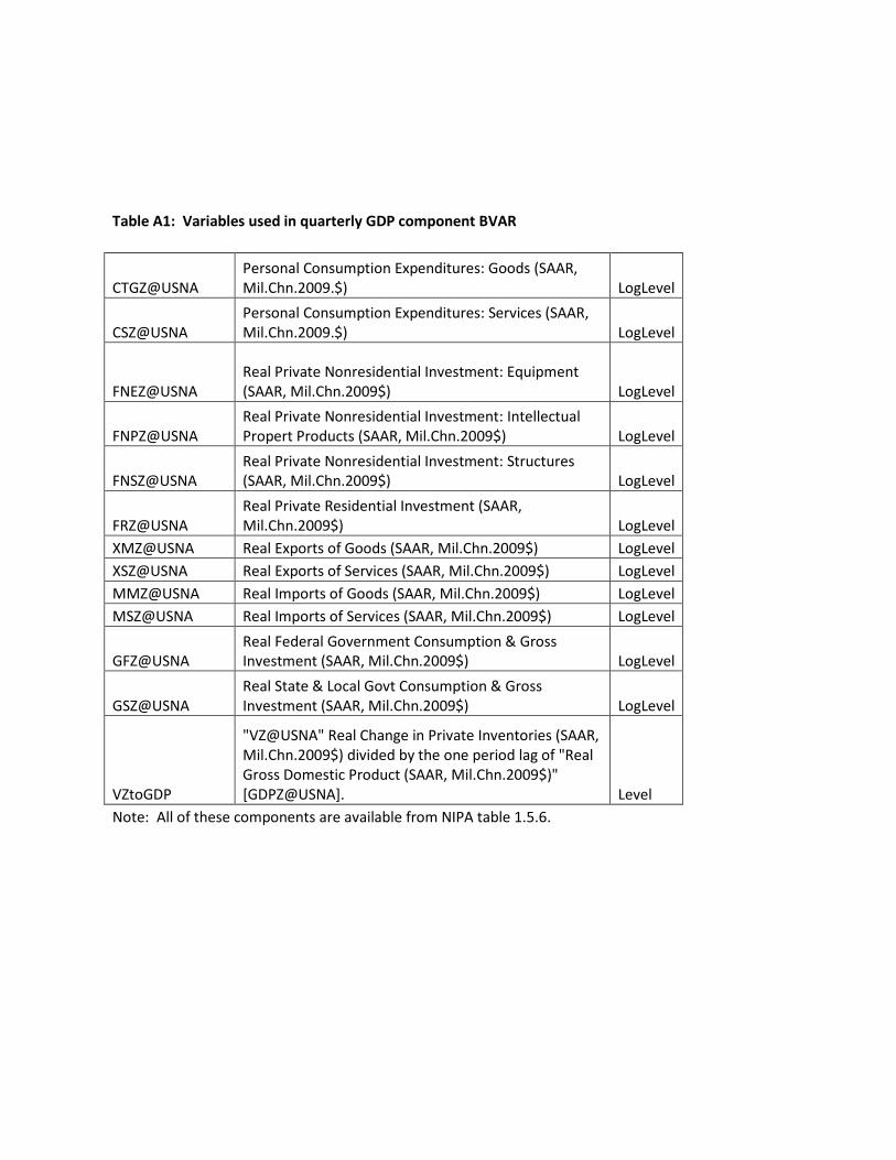
Table A1: Variables used in quarterly GDP component BVAR

CTGZ@USNA

Personal Consumption Expenditures: Goods (SAAR, Mil.Chn.2009.$) LogLevel

CSZ@USNA Personal Consumption Expenditures: Services (SAAR, Mil.Chn.2009.$) LogLevel

FNEZ@USNA Real Private Nonresidential Investment: Equipment (SAAR, Mil.Chn.2009$) LogLevel

FNPZ@USNA Real Private Nonresidential Investment: Intellectual Propert Products (SAAR, Mil.Chn.2009$) LogLevel

FNSZ@USNA Real Private Nonresidential Investment: Structures (SAAR, Mil.Chn.2009$) LogLevel

FRZ@USNA Real Private Residential Investment (SAAR, Mil.Chn.2009$) LogLevel

XMZ@USNA Real Exports of Goods (SAAR, Mil.Chn.2009$) LogLevel XSZ@USNA Real Exports of Services (SAAR, Mil.Chn.2009$) LogLevel MMZ@USNA Real Imports of Goods (SAAR, Mil.Chn.2009$) LogLevel MSZ@USNA Real Imports of Services (SAAR, Mil.Chn.2009$) LogLevel

GFZ@USNA Real Federal Government Consumption & Gross Investment (SAAR, Mil.Chn.2009$) LogLevel

GSZ@USNA Real State & Local Govt Consumption & Gross Investment (SAAR, Mil.Chn.2009$) LogLevel

VZtoGDP

"VZ@USNA" Real Change in Private Inventories (SAAR, Mil.Chn.2009$) divided by the one period lag of "Real Gross Domestic Product (SAAR, Mil.Chn.2009$)" [GDPZ@USNA]. Level

Note: All of these components are available from NIPA table 1.5.6.

Table A2: Variables used in monthly price BVAR

Variable Name Variable Descrption Transformation PCU@USECON CPI-U: All Items (SA, 1982-84=100) LogDiff PCUSLFE@USECON CPI-U: All Items Less Food and Energy (SA, 1982-84=100) LogDiff PCUSND@USECON CPI-U: Nondurables (SA, 1982-84=100) LogDiff PCUSSLE@USECON CPI-U: Services Less Energy Services (SA, 1982-84=100) LogDiff UH@CPIDATA CPI-U: Housing (SA, 1982-84=100) LogDiff SP2620@PPI PPI: Nonmanufacturing Industries (SA, 1982=100) LogDiff SP3000@USECON PPI: Finished Goods (SA, 1982=100) LogDiff

SP2900@PPI PPI: Intermediate Materials Less Food and Energy (SA, 1982=100) LogDiff

sa(RMFG@PPIR) PPI: Manufacturing (Dec-84=100) - Seasonal Adjustment, All LogDiff

PZALL@USECON KR-CRB Spot Commodity Price Index: All Commodities (1967=100) LogDiff

PZTEXP@USECON Spot Oil Price: West Texas Intermediate [Prior'82=Posted Price] ($/Barrel) LogDiff

NAPMPI@USECON ISM: Mfg: Prices Index (NSA, 50+ = Econ Expand) Lev

SpliceRetailTradeDeflator

Sales Price Deflator: Retail Trade (SA, 2005=100) "DTSR@USNA", spliced together with SIC based equivalent DTSR1@USNA before 1997. LogDiff

SpliceWholesaleTradeDeflator

Sales Price Deflator: Merchant Wholesale Trade Industries (SA, 2005=100) "DTSWM@USNA", spliced together with SIC based equivalent DTSW1@USNA before 1997. LogDiff

SpliceManTradeDeflator

Sales Price Deflator: Manufacturing Industries (SA, 2005=100), "DTSM@USNA" spliced together with SIC based equivalent "DTSM1@USNA" before 1997. LogDiff

SplicedMedian

FRB Cleveland Median CPI (SAAR, %chg) "CLEVFED@USECON" spliced together with discontinued median before 1983 CLEVM@USECON. LogDiff

SplicedTrim

FRB Cleveland 16% Trimmed-Mean CPI (SAAR, %chg) "CLEVCPI@USECON" spliced together with discontinued trim before 1983 CLEVT@USECON. LogDiff

GOODSIMPORTPRICEsplice

Log difference is weighted average of log differences of detailed import price indexes from BLS. The weights are the previous quarter's import shares of these detailed components from NIPA Table 4.2.5. See text for a more detailed description. LogDiff

PXEA_USECONsplice

Where available use PXEA@USECON "Export Price Index: All Imports (NSA, 2000=100) ". However from 1982-1988 the index is not available each month and therefore it is interpolated with a combination of the quarterly Export price index in the NIPA accounts and the PPI for finished goods [SP3000@PPI]. Uses proportional Denton method for interpolation. LogDiff

ImpSvcDefmthA1

Constructed deflator for services imports. Constructed by regressing quarterly log change in NIPA services imports implicit price deflator on 3 terms. 1.) GOODSIMPORTPRICEsplice. 2.) The previous quarter's 4-quarter log change in this same implicit price deflator. 3.) A constant. LogDiff

ExpSvcDefmthA1

Constructed deflator for services exports. Constructed by regressing quarterly log change in NIPA services exports implicit price deflator on 3 terms. 1.) PXEA_USECONsplice 2.) The previous quarter's 4-quarter log change in this same implicit price deflator. 3.) A constant. LogDiff

CoreRealRetailPCEDefExFoodSvc

This is a constructed Fisher price index of the PCE components that have counterparts in the "retail sales control" ex food services group. The Haver tickers for nominal expenditure categories are [CDMTM@USNA CDFDM@USNA CDOM@USNA CDRGM@USNA CSFPM@USNA CNLM@USNA CNOOM@USNA] and the tickers for the real expenditure categories are [CDMTHM@USNA CDFDHM@USNA CDOHM@USNA CDRGHM@USNA CSFPHM@USNA CNLHM@USNA CNOOHM@USNA]. Prices are defined implicitly. When the Consumer Price Index release comes out, the index is updated by linking the detailed "retail control" PCE price components to their counterparts in the CPI. See Table A7. LogDiff

HerzonServicesExFoodDef Constructed Fisher price index for nonfood services LogDiff CSFPMDef Implicit PCE price deflator for food services LogDiff

CDMVUMDef Implicit PCE price deflator for net purchases of used motor vehicles LogDiff

CDMVNMDef Implicit price deflator for Personal Consumption Expenditures: New Motor Vehicles LogDiff

CNEMDef Implicit price deflator for Personal Consumption Expenditures: Gasoline and Other Energy Goods LogDiff

TornPriceNonResStrMth Constructed deflator for private nonresidential construction put-in-place. See appendix for description. LogDiff

CCIHD@USECON Houses under Construction: Price Deflator (NSA, 2005=100) LogDiff

ESComputerDefqtrInterpSplice

Quarterly investment price deflator for computers interpolated/extrapolated to a monthly frequency using combination of "PPI: Electronic Computers and Computer Equipment (NSA, Dec-98=100) - Seasonal Adjustment, All" [sa(P115@PPI)] and "PCE: Personal Computers & Peripheral Equip Price Index (SA, 2005=100)" [JCDFCPM@USNA]. Uses proportional Denton method for interpolation. LogDiff

SP3200@PPI PPI: Capital Equipment (SA, 1982=100) LogDiff

R5312101_PPIRInterp

PPI: Real Estate Agts, Nonresid Prop Sales/Brokerage Fees/Commiss. Starts in 1995, so backcasted before then with the implicit price deflator for brokers' commissions on residential structures [interpolated to monthly frequency] LogDiff

RBMRS_PPIRback

PPI: Net Material Inputs: Resid Maintnce/Repair Construction. Starts in 1986, so backcasted before then with the implicit price deflator for residential improvements [interpolated to monthly frequency]. LogDiff

CPIMajappSplice

CPI-U: Major Appliances (SA, Dec-97=100). Starts in 1997, so backcasted before then with PCE: Major Household Appliances Price Index. LogDiff

Table A3: Data releases used for GDP nowcast

Primary data release Source

GDP components forecasted directly from release

Reuters/University of Michigan Index of Consumer Sentiment Reuters/University of Michigan None**, ***

Philly Fed Business Outlook Survey Federal Reserve Bank of Philadelphia None**, ***

Conference Board Consumer Confidence The Conference Board None**, *** Chicago Fed Midwest Manufacturing Index

Federal Reserve Bank of Chicago None**

ISM Manufacturing Index Institute for Supply Management Change in private inventories

ISM Nonmanufacturing Index Institute for Supply Management None**, ***

BEA Unit Auto sales Bureau of Economic Analysis Real PCE New Motor Vehicles, Change in private inventories

Initital Unemployment Insurance Claims Bureau of Labor Statistics None**

Employment situation Bureau of Labor Statistics

Nonresidential software investment, Government spending, Change in private inventories

Wholesale Trade U.S. Census Bureau Change in private inventories

International Trade (FT900) U.S. Census Bureau Net exports, Equipment investment, Change in private inventories

U.S. Import and Export Price Indexes Bureau of Labor Statistics Net exports Monthly Treasury Statement U.S. Treasury Government spending

Retail trade and inventories U.S. Census Bureau Real PCE (retail control) spending, Change in private inventories

Producer Price Index Bureau of Labor Statistics Equipment investment, Change in private inventories

Industrial Production Federal Reserve Change in private inventories, Government spending

Consumer Price Index Bureau of Labor Statistics Real PCE (retail control) spending, Change in private inventories

New residential construction C20 (Housing Starts) U.S. Census Bureau Residential investment Existing Home Sales U.S. Census Bureau Residential investment

Advance Durable Goods Report U.S. Census Bureau Equipment investment, Change in private inventories

New Home Sales U.S. Census Bureau Residential investment Manufacturers' Shipments, Inventories, and Orders U.S. Census Bureau

Equipment investment, Change in private inventories

Construction spending (C30) U.S. Census Bureau

Residential investment and nonresidential structures investment

Manufactured Homes Survey U.S. Census Bureau Residential investment Personal income and outlays Bureau of Economic Analysis Real PCE S&P 500 Index Standard and Poors None**

** Although not used to directly forecast any of the GDP components, it is used to estimate a latent factor (similar to the Chicago Fed National Activity Index) that is used to indirectly forecast many of the GDP components.

*** The most recent value of the series is not used to update the latent factor until the ISM Manufacturing Index is released

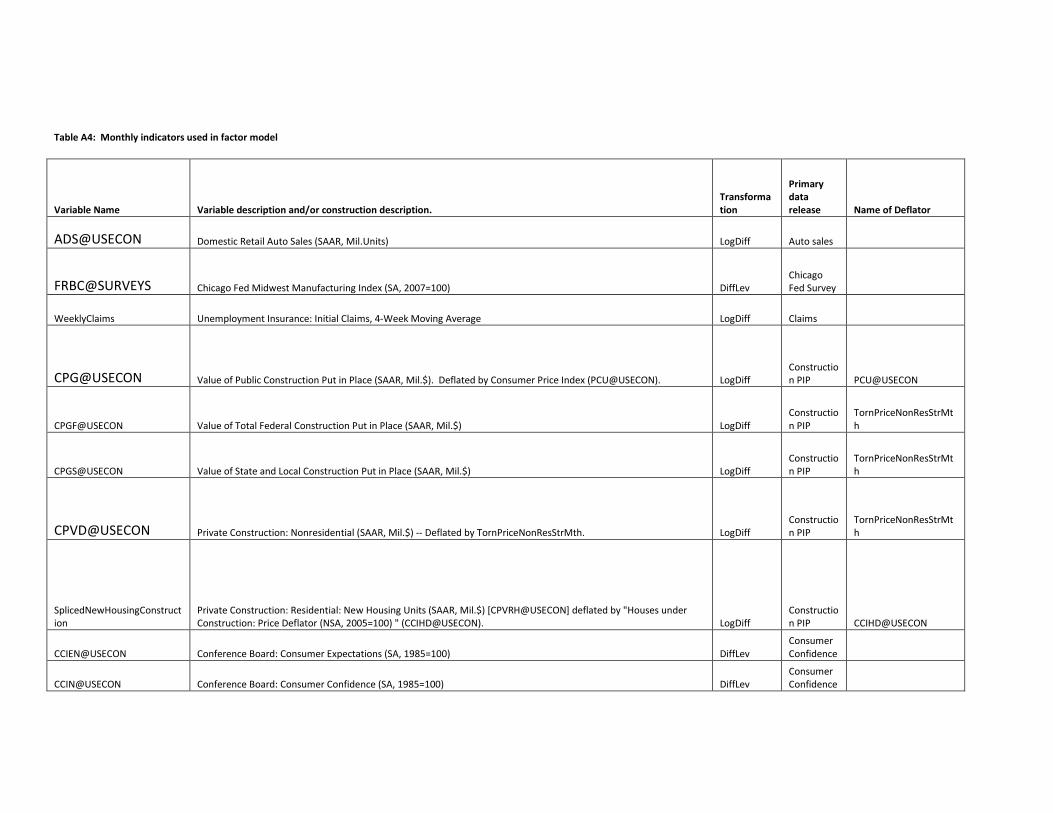
Table A4: Monthly indicators used in factor model

Variable Name Variable description and/or construction description. Transformation

Primary data release Name of Deflator

ADS@USECON Domestic Retail Auto Sales (SAAR, Mil.Units) LogDiff Auto sales

FRBC@SURVEYS Chicago Fed Midwest Manufacturing Index (SA, 2007=100) DiffLev Chicago Fed Survey

WeeklyClaims Unemployment Insurance: Initial Claims, 4-Week Moving Average LogDiff Claims

CPG@USECON Value of Public Construction Put in Place (SAAR, Mil.$). Deflated by Consumer Price Index (PCU@USECON). LogDiff Construction PIP PCU@USECON

CPGF@USECON Value of Total Federal Construction Put in Place (SAAR, Mil.$) LogDiff Construction PIP

TornPriceNonResStrMth

CPGS@USECON Value of State and Local Construction Put in Place (SAAR, Mil.$) LogDiff Construction PIP

TornPriceNonResStrMth

CPVD@USECON Private Construction: Nonresidential (SAAR, Mil.$) -- Deflated by TornPriceNonResStrMth. LogDiff Construction PIP

TornPriceNonResStrMth

SplicedNewHousingConstruction

Private Construction: Residential: New Housing Units (SAAR, Mil.$) [CPVRH@USECON] deflated by "Houses under Construction: Price Deflator (NSA, 2005=100) " (CCIHD@USECON). LogDiff

Construction PIP CCIHD@USECON

CCIEN@USECON Conference Board: Consumer Expectations (SA, 1985=100) DiffLev Consumer Confidence

CCIN@USECON Conference Board: Consumer Confidence (SA, 1985=100) DiffLev Consumer Confidence

CCIPSN@USECON Conference Board: Consumer Confidence Present Situation (SA, 1985=100) DiffLev Consumer Confidence

SplicedMichCur University of Michigan: Current Economic Conditions (NSA, Q1-66=100) -- CCOND@USECON. Pre 1978 survey was updated lower than monthly frequency; these observations are linearly interpolated. DiffLev

Consumer Sentiment

SplicedMichExp University of Michigan: Consumer Expectations (NSA, Q1-66=100) -- CEXP@USECON. Pre 1978 survey was updated lower than monthly frequency; these observations are linearly interpolated. DiffLev

Consumer Sentiment

SplicedMichSent University of Michigan: Consumer Sentiment (NSA, Q1-66=100) -- CSENT@USECON. Pre 1978 survey was updated lower than monthly frequency; these observations are linearly interpolated. DiffLev

Consumer Sentiment

LACONSA@USECON All Employees: Construction (SA, Thous) LogDiff Employment

LAD61A@USECON All Employees: Construction of Residential Buildings (SA, Thous) LogDiff Employment

LADURGA@USECON All Employees: Durable Goods Manufacturing (SA, Thous) LogDiff Employment

LAEDUHA@USECON All Employees: Education & Health Services (SA, Thous) LogDiff Employment

LAFGDA@LABOR All Employees: Department of Defense (SA, Thous) LogDiff Employment

LAFGOVA@USECON All Employees: Federal Government (SA, Thous) LogDiff Employment

LAFIREA@USECON All Employees: Financial Activities (SA, Thous) LogDiff Employment

LAGOODA@USECON All Employees: Goods-producing Industries (SA, Thous) LogDiff Employment

LALEIHA@USECON All Employees: Leisure & Hospitality (SA, Thous) LogDiff Employment

LAMANUA@USECON All Employees: Manufacturing (SA, Thous) LogDiff Employment

LAMINGA@USECON All Employees: Mining (SA, Thous) LogDiff Employment

LANAGRA@USECON All Employees: Total Nonfarm (SA, Thous) LogDiff Employment

LANDURA@USECON All Employees: Nondurable Goods Manufacturing (SA, Thous) LogDiff Employment

LAP15A@USECON All Employees: Computer Systems Design & Related Services (SA, Thous) LogDiff Employment

LAPBSVA@USECON All Employees: Professional & Business Services (SA, Thous) LogDiff Employment

LAPTSVA@USECON All Employees: Professional & Technical Services (SA, Thous) LogDiff Employment

LAPRIVA@USECON All Employees: Total Private Industries (SA, Thous) LogDiff Employment

LAPSRVA@USECON All Employees: Private Service-providing Industries (SA, Thous) LogDiff Employment

LARTRDA@USECON All Employees: Retail Trade (SA, Thous) LogDiff Employment

LASRVOA@USECON All Employees: Other Services (SA, Thous) LogDiff Employment

LAWTRDA@USECON All Employees: Wholesale Trade (SA, Thous) LogDiff Employment

LE@USECON Civilian Employment: Sixteen Years & Over (SA, Thous) LogDiff Employment

LENA@USECON Civilian Employment: Nonagricultural Industries: 16 yr + (SA, Thous) LogDiff Employment

LFPRUnround Civilian Labor Force: 16 yr + (SA, Thous) -- LF@USECON, series is divided by size of population. LogDiff Employment

LOMANUA@USECON Average Weekly Hours: Prod & Nonsupervisory: Overtime: Manufacturing (SA, Hrs) DiffLev Employment

LoserOnLayoff Civilians Unemployed: Job Losers On Layoff (SA, Thous.) -- LUJLL@USECON, series is divided by size of labor force. DiffLev Employment

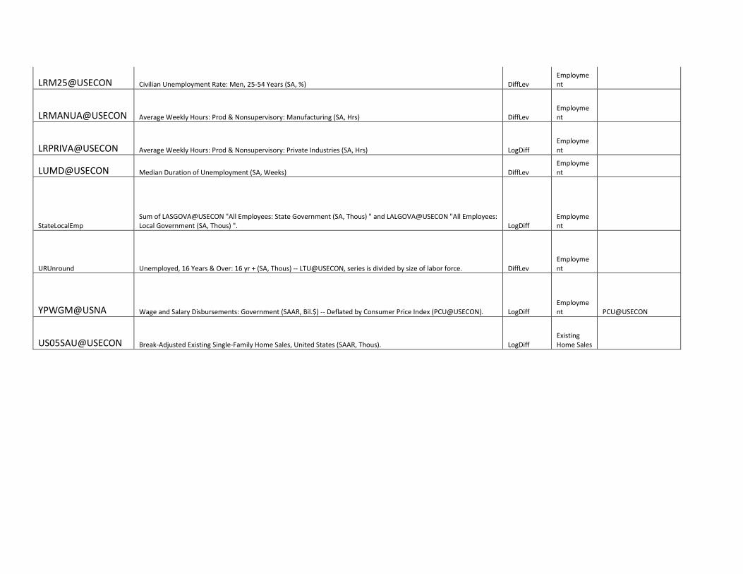
LRM25@USECON Civilian Unemployment Rate: Men, 25-54 Years (SA, %) DiffLev Employment

LRMANUA@USECON Average Weekly Hours: Prod & Nonsupervisory: Manufacturing (SA, Hrs) DiffLev Employment

LRPRIVA@USECON Average Weekly Hours: Prod & Nonsupervisory: Private Industries (SA, Hrs) LogDiff Employment

LUMD@USECON Median Duration of Unemployment (SA, Weeks) DiffLev Employment

StateLocalEmp Sum of LASGOVA@USECON "All Employees: State Government (SA, Thous) " and LALGOVA@USECON "All Employees: Local Government (SA, Thous) ". LogDiff

Employment

URUnround Unemployed, 16 Years & Over: 16 yr + (SA, Thous) -- LTU@USECON, series is divided by size of labor force. DiffLev Employment

YPWGM@USNA Wage and Salary Disbursements: Government (SAAR, Bil.$) -- Deflated by Consumer Price Index (PCU@USECON). LogDiff Employment PCU@USECON

US05SAU@USECON Break-Adjusted Existing Single-Family Home Sales, United States (SAAR, Thous). LogDiff Existing Home Sales

valExHomeSales

Nominal value is "existing single-family home sales" from National Association of Realtors (NAR) times the median sales price of existing single-family homes also from the NAR. The sales prices are NSA, so we seasonally adjust them with Haver's default settings. This constructed nominal sales value is deflated by the industry PPI for "PPI: Real Estate Agents: Residential Property Sales, Brokerage Fees, and Commissions" [NAICS code 5312101] from the Table 5 of the PPI release. LogDiff

Existing Home Sales R5312101@PPIRInterp

HPT@USECON New Pvt Housing Units Authorized by Building Permit (SAAR, Thous.Units) DiffLev Housing Starts

HST@USECON Housing Starts (SAAR, Thous.Units) DiffLev Housing Starts

HST1@USECON Housing Starts: 1 Unit (SAAR, Thous.Units) DiffLev Housing Starts

HSTM@USECON Housing Starts: Total Multifamily (SAAR, Thous.Units) DiffLev Housing Starts

HSTMW@USECON Housing Starts: Midwest (SAAR, Thous.Units) DiffLev Housing Starts

HSTNE@USECON Housing Starts: Northeast (SAAR, Thous.Units) DiffLev Housing Starts

HSTS@USECON Housing Starts: South (SAAR, Thous.Units) DiffLev Housing Starts

HSTW@USECON Housing Starts: West (SAAR, Thous.Units) DiffLev Housing Starts

NomSingleStarts

Housing Starts: 1 Unit (HST1@USECON) multiplied by "New 1-Family Houses: Average Sales Price (Dollars) - Seasonal Adjustment, All" (sa(HN1PA@USECON)). Series is then deflated by "Houses under Construction: Price Deflator (NSA, 2005=100)" (CCIHD@USECON). LogDiff

Housing Starts CCIHD@USECON

CoreCapGoodsExports

Exports: Capital Goods, except Automotive (SA, Mil.$) TXG2@USINT. Then exports for other noncore categories are subtracted. (TX21300@USINT,TX21301@USINT,TX22000@USINT,TX22010@USINT,TX22020@USINT,TX22220@USINT,TX21320@USINT,TX21100@USINT, and TX20005@USINT) Series is then deflated by PPI: Capital Equipment (SA, 1982=100) [SP3200@PPI]. LogDiff

International Trade SP3200@PPI

CoreCapGoodsImports

Imports: Capital Goods, except Automotive (SA, Mil.$) TMG2@USINT. Then exports for other noncore categories are subtracted. (TM21300@USINT,TM21301@USINT,TM22000@USINT,TM22010@USINT,TM22020@USINT,TM22220@USINT,TM21320@USINT,TM21100@USINT, and TM20005@USINT) Series is then deflated by PPI: Capital Equipment (SA, 1982=100) [SP3200@PPI]. LogDiff

International Trade SP3200@PPI

SplicedExportsComputersAndRelated

Nominal series is sum of exports of "computers" and "computer accessories" from from Exhibit 7 of Census international trade release (FT900). Nominal series is deflated by "Atkeson-Ohanian" extrapolator of quarterly price deflator for comupters and peripherals investment. See text for description of the extrapolation method. LogDiff

International Trade

ESComputerDefmthAO [ "Atkeson-Ohanian" extrapolator of quarterly price deflator for comupters and peripherals investment. See text for description of the extrapolation.]

SplicedGoodsExports Exports of goods on BOP basis from Census FT900 International Trade Release. FRED ticker BOPGEXP. Series not available before 1992, so backcast with "Exports, f.a.s.: Total Goods, Census Basis -- TMXA@USINT" LogDiff

International Trade PXEA@USECONsplice

SplicedGoodsImports Imports of goods on BOP basis from Census FT900 International Trade Release. FRED ticker BOPGIMP. Series not available before 1992, so backcast with "Imports, f.a.s.: Total Goods, Census Basis -- TMMA@USINT" LogDiff

International Trade PMEA@USECONsplice

SplicedImportsComputersAndRelated

Nominal series is sum of exports of "computers" and "computer accessories" from from Exhibit 7 of Census international trade release (FT900). Nominal series is deflated by ESComputerDefmthAO LogDiff

International Trade

ESComputerDefmthAO [ "Atkeson-Ohanian" extrapolator of quarterly price deflator for comupters and peripherals investment. See appendix for description of the extrapolation.]

SplicedServiceExports Exports of services on BOP basis from Census FT900 International Trade Release. FRED ticker BOPSEXP. Haver ticker BPXSVM@USECON LogDiff

International Trade ExpSvcDefmthA1

SplicedServiceImports Exports of services on BOP basis from Census FT900 International Trade Release. FRED ticker BOPSIMP. Haver ticker BPXSVX@USECON LogDiff

International Trade ImpSvcDefmthA1

CUMFG@IP Capacity Utilization: Manufacturing [SIC] (SA, % of Capacity) LogDiff IP

CUT@IP Capacity Utilization: Total Index (SA, % of Capacity) LogDiff IP

IP@IP IP: Total Index (SA, 2007=100) LogDiff IP

IP51@IP IP: Consumer Goods (SA, 2007=100) LogDiff IP

IP511@IP IP: Durable Consumer Goods (SA, 2007=100) LogDiff IP

IP512@IP IP: Nondurable Consumer Goods (SA, 2007=100) LogDiff IP

IP521@IP IP: Business Equipment (SA, 2007=100) LogDiff IP

IP53@IP IP: Materials (SA, 2007=100) LogDiff IP

IP54@IP IP: Nonindustrial Supplies (SA, 2007=100) LogDiff IP

IPB31@IP IP: Drilling Oil and Gas Wells (SA, 2007=100) LogDiff IP

IPFP@IP IP: Final Products {Mkt Group} (SA, 2007=100) LogDiff IP

IPMFG@IP IP: Manufacturing (SIC) (SA, 2007=100) LogDiff IP

IPTP@IP IP: Final Products and Nonindustrial Supplies (SA, 2007=100) LogDiff IP

NAPMC@USECON ISM Mfg: PMI Composite Index (SA, 50+ = Econ Expand) Lev ISM Manuf

NAPMEI@USECON ISM Mfg: Employment Index (SA, 50+ = Econ Expand) Lev ISM Manuf

NAPMII@USECON ISM Mfg: Inventories Index (SA, 50+ = Econ Expand) Lev ISM Manuf

NAPMNI@USECON ISM Mfg: New Orders Index (SA, 50+ = Econ Expand) Lev ISM Manuf

NAPMOI@USECON ISM Mfg: Production Index (SA, 50+ = Econ Expand) Lev ISM Manuf

NAPMVDI@USECON ISM Mfg: Supplier Deliveries Index (SA, 50+ = Slower) Lev ISM Manuf

NMFC@SURVEYS ISM Nonmanufacturing: NMI Composite Index (SA, 50+=Increasing) Lev ISM NonManuf

ASTOT@USECON Domestic plus Imported Retail Auto Sales (SAAR, Mil.Units) LogDiff

Light Weight Vehicle Sales

TLTSAR@USECON Total Truck Sales: Light, 0-14,000 Lbs GVW (SAAR, Mil.Units) LogDiff

Light Weight Vehicle Sales

BusShareTrucks

Business share of unit truck sales; constructed variable. Total unit light weight truck sales [business plus consumers] is from BEA [http://www.bea.gov/national/xls/gap_hist.xls] with FRED ticker LTRUCKSA. Consumer unit light weight truck sales is from NIPA table 7.2.5S. Share is 1 minus ratio of unit sales to consumer to total unit sales DiffLev

Light Weight Vehicle Sales + NIPA Underlying Detail 7.2.5S

CoreCapGoodsShipments

Mfrs' Shipments: Nondefense Capital Goods ex Aircraft (SA, Mil.$) minus computer shipments (NMSG41A@USECON, NMSG41B@USECON and NMSG41C@USECON). Series is then deflated by Series is then deflated by PPI: Capital Equipment (SA, 1982=100) [SP3200@PPI]. LogDiff

M3/Shipments SP3200@PPI

DefenseShipments "Manufacturers' Shipments: Defense Capital Goods (SA, Mil.$) " [MSCD@USECON] deflated by Consumer Price Index [PCU@USECON]. LogDiff

M3/Shipments PCU@USECON

HSM@USECON Manufacturers' Shipments of Mobile Homes (SAAR, Thous.Units) DiffLev M3/Shipments

ManInvShipRatio Manuf I/S ratio. NMI@USECON/NMS@USECON. Mfrs' Inventories: All Manufacturing Industries (EOP, SA, Mil.$) divided by Mfrs' Shipments: All Manufacturing Industries (SA, Mil.$) LogDiff

M3/Shipments

NMS@USECON Mfrs' Shipments: All Manufacturing Industries (SA, Mil.$). Converted to real by dividing by SpliceManTradeDeflator LogDiff M3/Shipments

SpliceManTradeDeflator

RealCapitalShipments Mfrs' Shipments: Nondefense Capital Goods ex Aircraft (SA, Mil.$) deflated by PPI: Capital Equipment (SA, 1982=100) (NMSCNX@USECON/SP3200@PPI) LogDiff

M3/Shipments

SplicedComputersShipments

Nominal series is sum of "Electronic Computers", "Computer Storage Devices", and "Other Computer Peripheral Eqpt" from Table 1 of full Census M3-2 report. These series are not included in the advance durable goods report (M3-1); in between M3-1 and M3-2 the latest month's values are extrapolated by "Computers & Electronic Products" shipments from the M3-1. Nominal series is deflated by "Atkeson-Ohanian" extrapolator of quarterly price deflator for comupters and peripherals investment. See appendix for description of the extrapolation. LogDiff

M3/Shipments

ESComputerDefmthAO [ "Atkeson-Ohanian" extrapolator of quarterly price deflator for comupters and peripherals investment. See text for description of the extrapolation.]

SplicedDurableGoodsOrders Constructed (Real) Manufacturers' New Orders: Durable Goods (SA, Mil.$). NAICS based nominal series is NMODG@USECON deflated by SP3200@PPI. LogDiff

M3/Shipments SP3200@PPI

NondefenseAircraftNetShipments

Constructed variable. Nominal shipments are "Mfrs' Shipments: Nondefense Aircraft & Parts" [From Census M3 Report -- FRED ticker ANAPVS] excluding shipments of "Electronic Computers", "Computer Storage Devices", and "Other Computer Peripheral Eqpt" from same M3 report. Net shipments subtract exports of Civilian Aircraft, Civilian Aircraft: Parts, Civilian Aircraft: Engines from Exhibit 7 of FT900 and add imports of these same categories. LogDiff

M3/Shipments + International Trade S142102@PPIextrap

MobileHomeVal

Nominal value is unit shipments of manufactured homes from the Census Bureau Manufactured Homes Survey (see http://www.census.gov/construction/mhs/mhsindex.html) times average sales price of manufactured homes from same survey. The sales price data are NSA, so we seasonally adjust them with Haver's default settings. Nominal mobile home shipments are deflated by the PPI for mobile homes [in Table 6 of PPI release]. LogDiff

Manufactured Homes Survey P155@PPI

HN1MT@USECON New 1-Family Houses For Sale: Months Supply (SA, Ratio) LogDiff New Home Sales

HN1SUS@USECON New 1-Family Houses For Sale: United States (SA, Thous) DiffLev New Home Sales

HN1US@USECON New 1-Family Houses Sold: United States (SAAR, Thous) DiffLev New Home Sales

valNewHomeSales

Nominal value is "New 1-Family Houses Sold" from the Census New Home Sales release [FRED ticker HSN1F] times the average sales price from table 1 of the same release. The sales price series is NSA, so we seasonally adjust it with Haver's default settings. This constructed nominal sales value is deflated by the industry PPI for "PPI: Real Estate Agents: Residential Property Sales, Brokerage Fees, and Commissions" [NAICS code 5312101] from the Table 5 of the release LogDiff

New Home Sales R5312101@PPIRInterp

ASCPU@USNA Autos: Consumer Dollars as a Percent of Final Sales (SA, %) DiffLev

NIPA Underlying Detail 7.2.5S

TSHSU@USNA Total Heavy Truck Sales [Over 14,000 lbs GVW] (SAAR, Mil.Units) LogDiff

NIPA Underlying Detail 7.2.5S

CBHM@USECON Real Personal Consumption Expenditures (SAAR, Bil.Chn.2005$) LogDiff PCE/Personal Income

CDBHM@USECON Real Personal Consumption Expenditures: Durable Goods (SAAR, Bil.Chn.2005$) LogDiff PCE/Personal Income

CNBHM@USECON Real Personal Consumption Expenditures: Nondurable Goods (SAAR, Bil.Chn.2005$) LogDiff PCE/Personal Income

CSBHM@USECON Real Personal Consumption Expenditures: Services (SAAR, Bil.Chn.2005$) LogDiff PCE/Personal Income

YPDHM@USECON Real Disposable Personal Income (SAAR, Bil.Chn.2005$) LogDiff PCE/Personal Income

YPLTPMH@USECON Real Personal Income Less Transfer Payments (SAAR, Bil.Chn.2005$) LogDiff PCE/Personal Income

BOFGX@SURVEYS Philadelphia Fed Business Outlook Survey: Future Activity Index (SA, %Bal) Lev Philly Fed Survey

BOISM@SURVEYS Philly Fed Bus Outlook: Current Activity Diffusion Index, ISM-Adj (SA, >50=Inc) Lev Philly Fed Survey

CoreRetailSales Constructed (Real) Retail Sales & Food Serv Excl Auto, Gas Stations & Building Materials(SA, Mil.$). Nominal NAICS based series is NRSXMI47@USECON. Deflated by constructed Core Retail PCE Deflator. LogDiff Retail trade CoreRealRetailPCEDef

NRST@USECON Retail Sales & Food Services (SA, Mil.$) deflated by constructed retail trade deflator LogDiff Retail trade SpliceRetailTradeDeflator

RetailInvSalesRatio Inventory to sales ratio for retail: Total Excl Motor Vehicle & Parts Dealers NRIXM@USECON/NRSXM@USECON LogDiff Retail trade

RetSalesResEquip

Nominal values from monthly retail trade relase [NAICS code 442 and NAICS codes 44311+44313]. Appliance T.V. and camera store sales are released with a 1-month lag, so they are extraplated with electronics and appliance store sales [NAICS code 443]. Nominal series deflated by CPI for major appliances. LogDiff Retail trade CPIMajappSplice

SplicedBuildingMaterials Retail Sales: Building Materials, Garden Equipment & Supply Dealers (SA, Mil.$) -- (NRSI4@USECON). LogDiff Retail trade ImprovementsDef**

SDY5COMM@USECON S&P: Composite 500, Dividend Yield (%) DiffLev S&P 500

SP500@USECON Stock Price Index: Standard & Poor's 500 Composite (1941-43=10) LogDiff S&P 500 PCU@USECON

saFTO@USECON Federal Outlays (Mil.$) - Seasonal Adjustment, All LogDiff Treasury PCU@USECON

saFTOD@USECON Federal Outlays: National Defense (Mil.$) - Seasonal Adjustment, All LogDiff Treasury PCU@USECON

NWSH@USECON Merchant Wholesalers: Sales: Total (SA, Mil.$). Deflated by Wholesale Trade Deflator. LogDiff Wholesale SpliceWholesaleTradeDeflator

WholeSaleInvSalesRatio Merchant Wholesalers: Inventory to sales ratio. LogDiff Wholesale

**ImprovementsDef is geometric mean of 3 series: 1.) Census price index for "New Single-Family Houses Under Construction" CCIHD@USECON. 2.) Industry PPI [Table 9] for Net Material Inputs: Residential Maintenance&Repair Construction RBMRS@PPIR 3.) Price index constructed with "Atkeson-Ohanian" extrapolation of 4-quarter percen change in Employment Cost Index for Construction. LSPIGC@USECON

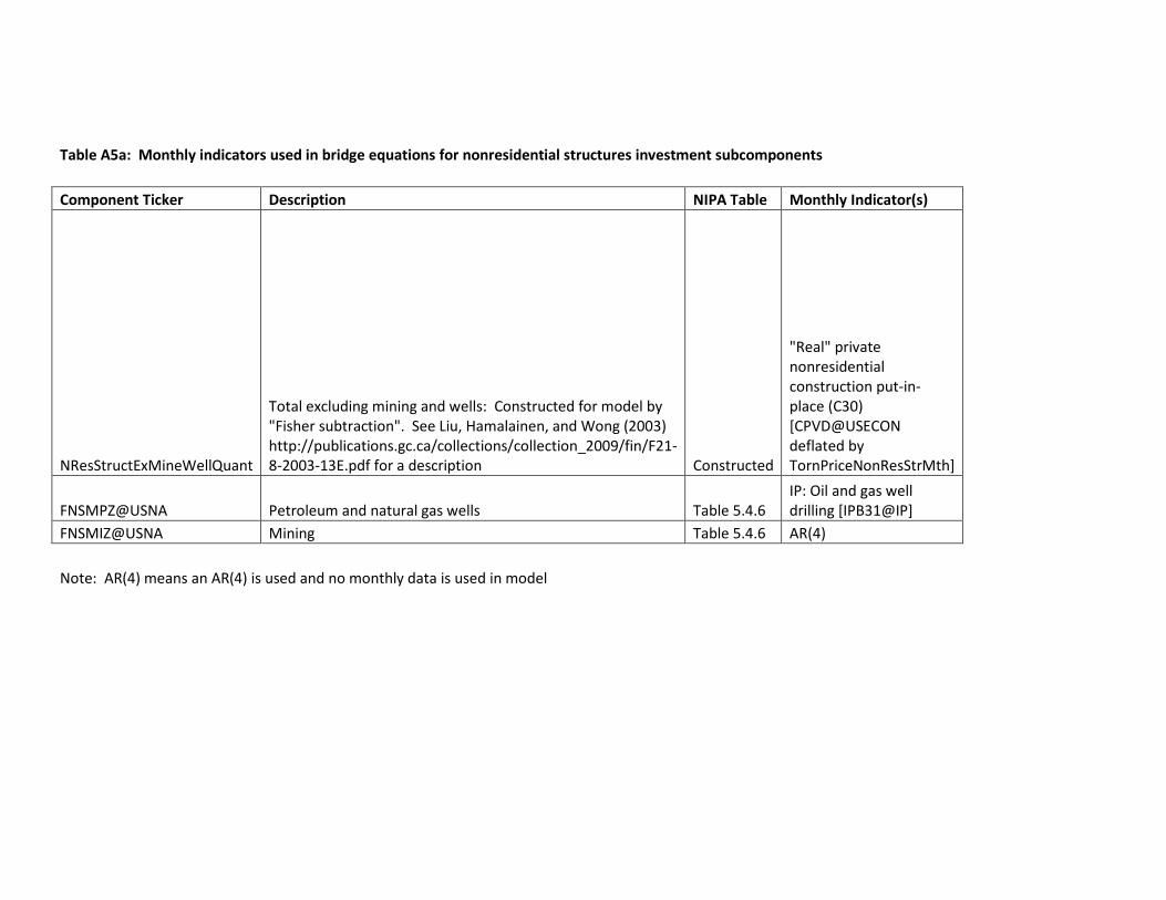
Table A5a: Monthly indicators used in bridge equations for nonresidential structures investment subcomponents

Component Ticker Description NIPA Table Monthly Indicator(s)

NResStructExMineWellQuant

Total excluding mining and wells: Constructed for model by "Fisher subtraction". See Liu, Hamalainen, and Wong (2003) http://publications.gc.ca/collections/collection_2009/fin/F21-8-2003-13E.pdf for a description Constructed

"Real" private nonresidential construction put-in-place (C30) [CPVD@USECON deflated by TornPriceNonResStrMth]

FNSMPZ@USNA Petroleum and natural gas wells Table 5.4.6 IP: Oil and gas well drilling [IPB31@IP]

FNSMIZ@USNA Mining Table 5.4.6 AR(4)

Note: AR(4) means an AR(4) is used and no monthly data is used in model

Table A5b: Monthly indicators used in bridge equations for residential investment subcomponents

Component Ticker Description NIPA Table Monthly Indicator(s)

FRSPZ@USNA Permanent-site Table 5.3.6

"Real" private new housing construction (VPIP) [SplicedNewHousingConstruction/CCHID@USECON]: Nominal series is sum of spending on new single family and new multifamily housing construction from Table 2 Census C30 release. In the interim period between the "New Residential Construction" housing starts release and the C30 value put in place release, we update this series in the model using the method described in the appendix.

FRSHMZ@USNA Manufactured homes Table 5.4.6U "Real" value of mobile home shipments [MobileHomeVal/P155@PPI] FRSHDZ@USNA Dormitories Table 5.4.6U AR(4)

FRSBKZ@USNA Brokerage commissions Table 5.4.6U "Real" value of new and existing home sales [valExHomeSales + valNewHomeSales]/R5312101_PPIRInterp

FRSINZ@USNA Improvements Table 5.4.6U

"Real" Retail Sales: Building Materials, Garden Equipment & Supply Dealers [SplicedBuildingMaterials deflated by geometric mean of 3 series deflated by geometric mean of 3 series: 1.) Census price index for "New Single-Family Houses Under Construction" CCIHD@USECON. 2.) Industry PPI [Table 9] for Net Material Inputs: Residential Maintenance&Repair Construction RBMRS@PPIR 3.) Price index constructed with "Atkeson-Ohanian" extrapolation of 4-quarter percen change in Employment Cost Index for Construction. LSPIGC@USECON]

FREZ@USNA Residential equipment Table 5.3.6

"Real" Retail Sales: Appliance, Television, and Camera Stores + Furniture & Home Furniture Stores [RetSalesResEquip/CPIMajappSplice]

Note: AR(4) means an AR(4) is used and no monthly data is used in model

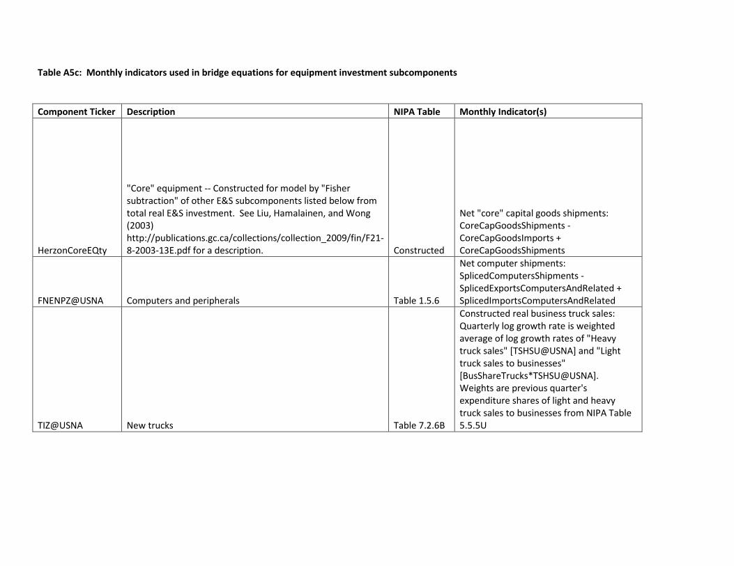
Table A5c: Monthly indicators used in bridge equations for equipment investment subcomponents

Component Ticker Description NIPA Table Monthly Indicator(s)

HerzonCoreEQty

"Core" equipment -- Constructed for model by "Fisher subtraction" of other E&S subcomponents listed below from total real E&S investment. See Liu, Hamalainen, and Wong (2003) http://publications.gc.ca/collections/collection_2009/fin/F21-8-2003-13E.pdf for a description. Constructed

Net "core" capital goods shipments: CoreCapGoodsShipments - CoreCapGoodsImports + CoreCapGoodsShipments

FNENPZ@USNA Computers and peripherals Table 1.5.6

Net computer shipments: SplicedComputersShipments - SplicedExportsComputersAndRelated + SplicedImportsComputersAndRelated

TIZ@USNA New trucks Table 7.2.6B

Constructed real business truck sales: Quarterly log growth rate is weighted average of log growth rates of "Heavy truck sales" [TSHSU@USNA] and "Light truck sales to businesses" [BusShareTrucks*TSHSU@USNA]. Weights are previous quarter's expenditure shares of light and heavy truck sales to businesses from NIPA Table 5.5.5U

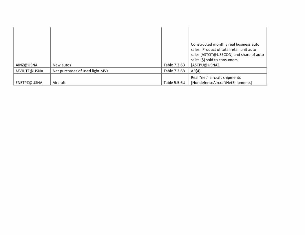
AINZ@USNA New autos Table 7.2.6B

Constructed monthly real business auto sales. Product of total retail unit auto sales [ASTOT@USECON] and share of auto sales ($) sold to consumers [ASCPU@USNA].

MVIUTZ@USNA Net purchases of used light MVs Table 7.2.6B AR(4)

FNETPZ@USNA Aircraft Table 5.5.6U Real "net" aircraft shipments [NondefenseAircraftNetShipments]

Table A5d: Monthly indicators used in bridge equations for federal government expenditures subcomponents

Component Ticker Description NIPA Table(s) Monthly Indicator(s) GFZ@USNA Federal government spending National Defense

GFDESLZ@USNA Real Compensation of Employees: Military Table 3.11.6 AR(4)

GFDESVZ@USNA Real Compensation of Employees: Civilian Table 3.11.6 Payroll Employment: Department of Defense (Civilian) [LAFGDA@LABOR]

GFDSFZ@USNA Real Consumption of Govt Fixed Capital Table 3.11.6 AR(4)

NatDefenseTreasCatsQty

(Intermediate Durables+Svcs) + (Total Investment): Constructed chain-weighted aggregate.

Table 3.11.6+3.9.6

Treasury statement: National Defense Outlays (SA, Deflate by CPI) [saFTOD@USECON/PCU@USECON]

GFDENZ@USNA Intermediate Nondurables Table 3.11.6 AR(4) GDOAIZ@USNA (-)Own account investment Table 3.11.6 AR(4) GDOSSZ@USNA (-)Sales to other sectors Table 3.11.6 AR(4) Nondefense

GGNESZ@USNA Real Compensation of Employees Table 3.10.6 Nondefense payroll federal govt employment [LAFGOVA@USECON - LAFGDA@USECON]

GFNSFZ@USNA Real Consumption of Govt Fixed Capital Table 3.10.6 AR(4)

GFNEDZ@USNA Intermediate Durables Table 3.10.6 Treasury statement: Total Outlays (SA, Deflate by CPI) [saFTO@USECON/PCU@USECON]

GFNENZ@USNA Intermediate Nondurables Table 3.10.6 Treasury statement: Total Outlays (SA, Deflate by CPI) [saFTO@USECON/PCU@USECON]

GFNESZ@USNA Intermediate Services Table 3.10.6 AR(4) GNOAIZ@USNA (-)Own account investment Table 3.10.6 AR(4) GNOSSZ@USNA (-)Sales to other sectors Table 3.10.6 AR(4)

GFNISZ@USNA Structures investment Table 3.9.6 "Real" Value of Federal Construction Put in Place [CPGF@USECON/TornPriceNonResStrMth]

GFNIEZ@USNA Equipment+Software investment Table 3.9.6 AR(4)

Note: AR(4) means an AR(4) is used and no monthly data is used in model

Table A5e: Monthly indicators used in bridge equations for state+local govt expenditures subcomponents

Component Ticker Description

NIPA Table(s) Monthly Indicator(s)

GGSESZ@USNA Real compensation of general govt. employees Table 3.10.6

Payroll employment: state+local [StateLocalEmp = LASGOVA@USECON + LALGOVA@USECON]

GSESFZ@USNA Consumption of fixed capital Table 3.10.6 AR(4)

GSEPIZ@USNA Intermediate goods and svcs purchased Table 3.10.6 AR(4)

GSOAIZ@USNA (-)Own account investment Table 3.10.6 AR(4) GSOSSZ@USNA (-)Sales to other sectors Table 3.10.6 AR(4)

GSISZ@USNA Investment: Structures Table 3.9.6

"Real" State and Local Construction Put in Place [CPGS@USECON deflated by TornPriceNonResStrMth]

GSIEZ@USNA Investment: Equipment+Software Table 3.9.6 Industrial Production (Total) [IP@IP]

Note: AR(4) means an AR(4) is used and no monthly data is used in model

Table A5f: Monthly indicators used in bridge equations for intellectual proprty products investment subcomponents

Component Ticker Description NIPA Table Monthly Indicator(s)

FNPSZ@USNA Software Table 1.5.6 Prof. + bus. svcs employment [LAPBSVA@USECON]

FNPRZ@USNA Research and development Table 1.5.6 Prof. + technical svcs employment [LAPTSVA@USECON]

FNPEZ@USNA

Entertainment, literary, and artistic originals Table 1.5.6 AR(4)

Note: AR(4) means an AR(4) is used and no monthly data is used in model

Table A6: Component breakdown used to forecast consumption

Consumption Variable Name Consumption Variable Description Method for "nowcasting" latest month

GOODS

CDMVNHM@USNA

Personal Consumption Expenditures: New Motor Vehicles (SAAR, Mil.Chn.2005.$)

Latest number predicted with growth in share weighted average growth rates of unit auto sales to consumers [derived from ASTOT@USECON and ASCPU@USNA] and unit truck sales to consumers [derived from TLTSAR@USECON and BusShareTrucks].

CDMVUHM@USNA Real PCE: Net Purchases of Used Motor Vehicles No other monthly indicator used.

CoreRealRetailPCEQtyExFoodSvc

Personal Consumption Expenditures: Components that map into retail control basket less food services [retail trade series is NRSXMI47@USECON - NRSV2@USECON in Haver]

Latest number predicted with "Retail Sales & Food Serv Excl Auto, Gas Stations & Building Materials(SA, Mil.$) " less food services -- NRSXMI47@USECON - NRSV2@USECON --when available. NRSXMI47@USECON - NRSV2@USECON series is deflated by appropriate average of appropriate CPI components when available. Otherwise the deflator is forecast.

CNEHM@USNA

PCE: Gasoline & Other Energy Gds (SAAR, Mil.Chn.2005.$) No other monthly indicator used.

SERVICES

CSFPHM@USNA Real PCE: Purchased Meals & Beverages

Latest number predicted with "Retail sales food services & drinking places" -- NRSV2@USECON --when available. NRSV2@USECON series is deflated by appropriate average of appropriate CPI components when available. Otherwise the deflator is forecast.

HerzonServicesLessFoodQty

Constructed for model by "Fisher subtraction" of food services from total PCE services. Source data from NIPA tables 2.4.5U and 2.4.6U. See Liu, Hamalainen, and Wong (2003) http://publications.gc.ca/collections/collection_2009/fin/F21-8-2003-13E.pdf for a description of Fisher subtraction. No other monthly indicator used.

Table A7: CPI to PCE retail correspondence

CPI Price Component CPI Price Description PCE Price Component PCE Price Description

UTCT@CPIDATA CPI-U: Tires (SA, 1982-84=100) JCDMTTM@USNA Personal Consumption Expenditures: Tires Price Index (SA, 2009=100)

UTCOON@CPIDATA CPI-U: Vehicle Parts & Eqpt ex Tires (NSA, 1982-84=100) JCDMTVM@USNA

Personal Consumption Expenditures: Accessories & Parts Price Index(SA, 2009=100)

UHHF@CPIDATA CPI-U: Household Furniture & Bedding (SA, 1982-84=100) JCDFUM@USNA

Personal Consumption Expenditures: Furniture Price Index (SA, 2009=100)

UHHQCN@CPIDATA CPI-U: Clocks, Lamps and Decorator Items (NSA, 1982-84=100) JCDFOLM@USNA

PCE: Clock/Lamp/Lighting Fixture/Othr HH Decorative Item Price Idx(SA, 2009=100)

UHHWFN@CPIDATA CPI-U: Floor Coverings (NSA, Dec-97=100) JCDFOFM@USNA

PCE: Carpets & Other Floor Coverings Price Index (SA, 2009=100)

UHHWW@CPIDATA CPI-U: Window Coverings (SA, Dec1997=100) JCDFOTM@USNA

Personal Consumption Expenditures: Window Coverings Price Index (SA, 2009=100)

UHHPM@CPIDATA CPI-U: Major appliances(SA, Dec-97=100) JCDFKKM@USNA

PCE: Major Household Appliances Price Index (SA, 2009=100)

UHHPO@CPIDATA CPI-U: Other Household Appliances (SA, Dec-97=100) JCDFKSM@USNA

PCE: Small Elec Household Appliances Price Index (SA, 2009=100)

UHHQDN@CPIDATA CPI-U: Dishes and Flatware (NSA, Dec-97=100) JCDFGDM@USNA

Personal Consumption Expenditures: Dishes and Flatware Price Index(SA, 2009=100)

UHHQK@CPIDATA CPI-U: Nonelectric Cookware and Tableware (SA, Dec1997=100) JCDFGKM@USNA

PCE: Nonelectric Cookware & Tableware Price Index (SA, 2009=100)

UHHTTN@CPIDATA CPI-U: Tools, Hardware and Supplies (NSA, Dec-97=100) JCDFSTM@USNA

PCE: Tools, Hardware & Supplies Price Index (SA, 2009=100)

UHHTQ@CPIDATA CPI-U: Outdoor Equipment and Supplies (SA, Dec-97=100) JCDFSLM@USNA

PCE: Outdoor Equip & Supplies Price Index (SA, 2009=100)

UEVT@CPIDATA CPI-U: Televisions (SA, 1982-84=100) JCDFTVM@USNA Personal Consumption Expenditures: Televisions Price Index (SA, 2009=100)

UEVQ@CPIDATA CPI-U: Other Video Equipment (SA, Dec-97=100) JCDFTOM@USNA

Personal Consumption Expenditures: Other Video Equip Price Index (SA, 2009=100)

UEVAN@CPIDATA CPI-U: Audio Equipment (NSA, 1982-84=100) JCDFTUM@USNA

Personal Consumption Expenditures: Audio Equipment Price Index (SA, 2009=100)

UEVADN@CPIDATA CPI-U: Audio Discs, Tapes & Other Media (NSA, Dec-97=100) JCDFTPM@USNA

PCE: Prerec/Blank Audio Disc/Tape/Digital Files/Download Price Idx(SA, 2009=100)

UEVDBN@CPIDATA CPI-U: Video Cassettes & Discs, Blank & Prerecorded (NSA, Dec-97=100, JCDFTCM@USNA

PCE: Video Cassettes & Discs, Blank & Prerecorded Price Index (SA, 2009=100)

UETPQ@CPIDATA CPI-U: Photographic Equipment (SA, Dec-97=100) JCDOWPM@USNA

Personal Consumption Expenditures: Photographic Equip Price Index (SA, 2009=100)

UDIIP@CPIDATA

CPI-U: Personal Computers and Peripheral Equipment (SA, Dec-07=100) JCDFCPM@USNA

PCE: Personal Computers & Peripheral Equip Price Index (SA, 2009=100)

UDIISN@CPIDATA CPI-U: Computer Software and Accessories (NSA, Dec 1997=100) JCDFCSM@USNA

PCE: Computer Software & Acc Price Index (SA, 2009=100)

UDIION@CPIDATA

CPI-U: Telephone Hardware/Calculators/Other Cons Info Items (NSA, Dec 1997=100) JCDFCOM@USNA

PCE: Calculators/Typewriters/Othr Info Processing Eqpt Price Idx(SA, 2009=100)

UEEON@CPIDATA CPI-U: Sports Equipment (NSA, 1982-84=100) JCDRSM@USNA

PCE: Sporting Equip, Supplies, Guns & Ammunition Price Index (SA, 2009=100)

UEES@CPIDATA CPI-U: Sport Vehicles including Bicycles (SA, 1982-84=100) JCDOWLM@USNA

Personal Consumption Expenditures: Motorcycles Price Index (SA, 2009=100)

UEES@CPIDATA CPI-U: Sport Vehicles including Bicycles (SA, 1982-84=100) JCDOWBM@USNA

Personal Consumption Expenditures: Bicycles & Acc Price Index (SA, 2009=100)

UEES@CPIDATA CPI-U: Sport Vehicles including Bicycles (SA, 1982-84=100) JCDBBBM@USNA

Personal Consumption Expenditures: Pleasure Boats Price Index (SA, 2009=100)

UEES@CPIDATA CPI-U: Sport Vehicles including Bicycles (SA, 1982-84=100) JCDBBPM@USNA

Personal Consumption Expenditures: Pleasure Aircraft Price Index (SA, 2009=100)

UEES@CPIDATA CPI-U: Sport Vehicles including Bicycles (SA, 1982-84=100) JCDBBOM@USNA

PCE: Other Recreational Vehicles Price Index (SA, 2009=100)

UERMN@CPIDATA CPI-U: Recreational Books (NSA, Dec-97=100) JCDRBM@USNA

Personal Consumption Expenditures: Recreational Books Price Index (SA, 2009=100)

UEGM@CPIDATA CPI-U: Music Instruments and Accessories (SA, Dec-97=100) JCDFTIM@USNA

Personal Consumption Expenditures: Musical Instruments Price Index(SA, 2009=100)

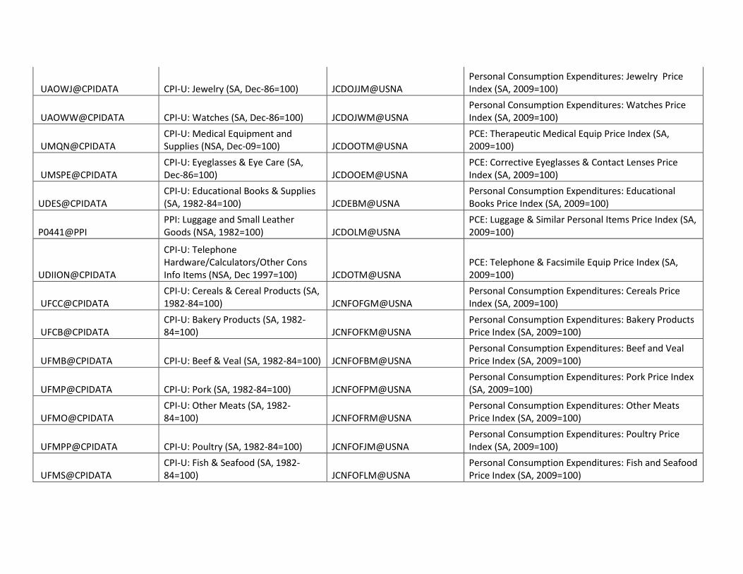
UAOWJ@CPIDATA CPI-U: Jewelry (SA, Dec-86=100) JCDOJJM@USNA Personal Consumption Expenditures: Jewelry Price Index (SA, 2009=100)

UAOWW@CPIDATA CPI-U: Watches (SA, Dec-86=100) JCDOJWM@USNA Personal Consumption Expenditures: Watches Price Index (SA, 2009=100)

UMQN@CPIDATA CPI-U: Medical Equipment and Supplies (NSA, Dec-09=100) JCDOOTM@USNA

PCE: Therapeutic Medical Equip Price Index (SA, 2009=100)

UMSPE@CPIDATA CPI-U: Eyeglasses & Eye Care (SA, Dec-86=100) JCDOOEM@USNA

PCE: Corrective Eyeglasses & Contact Lenses Price Index (SA, 2009=100)

UDES@CPIDATA CPI-U: Educational Books & Supplies (SA, 1982-84=100) JCDEBM@USNA

Personal Consumption Expenditures: Educational Books Price Index (SA, 2009=100)

P0441@PPI PPI: Luggage and Small Leather Goods (NSA, 1982=100) JCDOLM@USNA

PCE: Luggage & Similar Personal Items Price Index (SA, 2009=100)

UDIION@CPIDATA

CPI-U: Telephone Hardware/Calculators/Other Cons Info Items (NSA, Dec 1997=100) JCDOTM@USNA

PCE: Telephone & Facsimile Equip Price Index (SA, 2009=100)

UFCC@CPIDATA CPI-U: Cereals & Cereal Products (SA, 1982-84=100) JCNFOFGM@USNA

Personal Consumption Expenditures: Cereals Price Index (SA, 2009=100)

UFCB@CPIDATA CPI-U: Bakery Products (SA, 1982-84=100) JCNFOFKM@USNA

Personal Consumption Expenditures: Bakery Products Price Index (SA, 2009=100)

UFMB@CPIDATA CPI-U: Beef & Veal (SA, 1982-84=100) JCNFOFBM@USNA Personal Consumption Expenditures: Beef and Veal Price Index (SA, 2009=100)

UFMP@CPIDATA CPI-U: Pork (SA, 1982-84=100) JCNFOFPM@USNA Personal Consumption Expenditures: Pork Price Index (SA, 2009=100)

UFMO@CPIDATA CPI-U: Other Meats (SA, 1982-84=100) JCNFOFRM@USNA

Personal Consumption Expenditures: Other Meats Price Index (SA, 2009=100)

UFMPP@CPIDATA CPI-U: Poultry (SA, 1982-84=100) JCNFOFJM@USNA Personal Consumption Expenditures: Poultry Price Index (SA, 2009=100)

UFMS@CPIDATA CPI-U: Fish & Seafood (SA, 1982-84=100) JCNFOFLM@USNA

Personal Consumption Expenditures: Fish and Seafood Price Index (SA, 2009=100)

UFYF@CPIDATA CPI-U: Milk (SA, Dec-97=100) JCNFOFIM@USNA Personal Consumption Expenditures: Fresh Milk Price Index (SA, 2009=100)

UFYPC@CPIDATA CPI-U: Cheese and Related Products (SA, 1982-84=100) JCNFOFDM@USNA

PCE: Processed Dairy Products Price Index (SA, 2009=100)

UFME@CPIDATA CPI-U: Eggs (SA, 1982-84=100) JCNFOFEM@USNA Personal Consumption Expenditures: Eggs Price Index (SA, 2009=100)

UFOT@CPIDATA CPI-U: Fats and Oils (SA, 1982-84=100) JCNFOFWM@USNA

Personal Consumption Expenditures: Fats and Oils Price Index (SA, 2009=100)

UFFFF@CPIDATA CPI-U: Fresh Fruits (SA, 1982-84=100) JCNFOFFM@USNA Personal Consumption Expenditures: Fresh Fruit Price Index (SA, 2009=100)

UFFVF@CPIDATA CPI-U: Fresh Vegetables (SA, 1982-84=100) JCNFOFVM@USNA

Personal Consumption Expenditures: Fresh Vegetables Price Index (SA, 2009=100)

UFFP@CPIDATA CPI-U: Processed Fruits & Vegetables (SA, Dec-97=100) JCNFOFTM@USNA

PCE: Processed Fruits & Vegetables Price Index (SA, 2009=100)

UFOS@CPIDATA CPI-U: Sugar and Sweets (SA, 1982-84=100) JCNFOFSM@USNA

Personal Consumption Expenditures: Sugar and Sweets Price Index (SA, 2009=100)

UFH@CPIDATA CPI-U: Food At Home (SA, 1982-84=100) JCNFOFOM@USNA

PCE: Food Products, Not Elsewhere Classified Price Index (SA, 2009=100)

UFBVM@CPIDATA CPI-U: Beverage Materials Incl Coffee & Tea (SA, Dec-97=100) JCNFOFCM@USNA

PCE: Coffee, Tea & Other Beverage Mtls Price Index (SA, 2009=100)

UFBVJ@CPIDATA CPI-U: Juices & Nonalcoholic Drinks (SA, Dec-97=100) JCNFOFNM@USNA

PCE: Mineral Waters, Soft Drinks & Vegetable Juices Price Index (SA, 2009=100)

UABHD@CPIDATA CPI-U: Distilled Spirits At Home (SA, 1982-84=100) JCNFOLDM@USNA

Personal Consumption Expenditures: Spirits Price Index (SA, 2009=100)

UABHW@CPIDATA CPI-U: Wine At Home (SA, 1982-84=100) JCNFOLEM@USNA

Personal Consumption Expenditures: Wine Price Index (SA, 2009=100)

UABHB@CPIDATA CPI-U: Beer, Ale and Malt Beverages At Home (SA, 1982-84=100) JCNFOLBM@USNA

Personal Consumption Expenditures: Beer Price Index (SA, 2009=100)

UFH@CPIDATA CPI-U: Food At Home (SA, 1982-84=100) JCNFEFM@USNA

PCE: Food Produced & Consumed on Farms Price Index (SA, 2009=100)

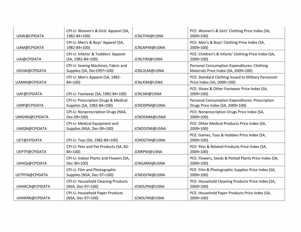
UAW@CPIDATA CPI-U: Women's & Girls' Apparel (SA, 1982-84=100) JCNLFFM@USNA

PCE: Women's & Girls' Clothing Price Index (SA, 2009=100)

UAM@CPIDATA CPI-U: Men's & Boys' Apparel (SA, 1982-84=100) JCNLMFM@USNA

PCE: Men's & Boys' Clothing Price Index (SA, 2009=100)

UAI@CPIDATA CPI-U: Infants' & Toddlers' Apparel (SA, 1982-84=100) JCNLFIM@USNA

PCE: Children's & Infants' Clothing Price Index (SA, 2009=100)

UEGW@CPIDATA CPI-U: Sewing Machines, Fabric and Supplies (SA, Dec1997=100) JCNLOLM@USNA

Personal Consumption Expenditures: Clothing Materials Price Index (SA, 2009=100)

UAMM@CPIDATA CPI-U: Men's Apparel (SA, 1982-84=100) JCNLXIM@USNA

PCE: Standard Clothing Issued to Military Personnel Price Index (SA, 2009=100)

UAF@CPIDATA CPI-U: Footwear (SA, 1982-84=100) JCNLSM@USNA PCE: Shoes & Other Footwear Price Index (SA, 2009=100)

UMP@CPIDATA CPI-U: Prescription Drugs & Medical Supplies (SA, 1982-84=100) JCNODPM@USNA

Personal Consumption Expenditures: Prescription Drugs Price Index (SA, 2009=100)

UMGNN@CPIDATA CPI-U: Nonprescription Drugs (NSA, Dec-09=100) JCNODNM@USNA

PCE: Nonprescription Drugs Price Index (SA, 2009=100)

UMQN@CPIDATA CPI-U: Medical Equipment and Supplies (NSA, Dec-09=100) JCNODOM@USNA

PCE: Other Medical Products Price Index (SA, 2009=100)

UET@CPIDATA CPI-U: Toys (SA, 1982-84=100) JCNOGTM@USNA PCE: Games, Toys & Hobbies Price Index (SA, 2009=100)

UEPTP@CPIDATA CPI-U: Pets and Pet Products (SA, 82-84=100) JCNRPM@USNA

PCE: Pets & Related Products Price Index (SA, 2009=100)

UHHQI@CPIDATA CPI-U: Indoor Plants and Flowers (SA, Dec-90=100) JCNGARM@USNA

PCE: Flowers, Seeds & Potted Plants Price Index (SA, 2009=100)

UETPFN@CPIDATA CPI-U: Film and Photographic Supplies (NSA, Dec-97=100) JCNOGFM@USNA

PCE: Film & Photographic Supplies Price Index (SA, 2009=100)

UHHKCN@CPIDATA CPI-U: Household Cleaning Products (NSA, Dec-97=100) JCNOLPM@USNA

PCE: Household Cleaning Products Price Index (SA, 2009=100)

UHHKRN@CPIDATA CPI-U: Household Paper Products (NSA, Dec-97=100) JCNOLFM@USNA

PCE: Household Paper Products Price Index (SA, 2009=100)

UHHWLN@CPIDATA CPI-U: Other Household Linens (NSA, Dec-97=100) JCNOLNM@USNA

Personal Consumption Expenditures: Household Linens Price Index (SA, 2009=100)

UEGW@CPIDATA CPI-U: Sewing Machines, Fabric and Supplies (SA, Dec1997=100) JCNOLSM@USNA

Personal Consumption Expenditures: Sewing Items Price Index (SA, 2009=100)

UHHKM@CPIDATA CPI-U: Miscellaneous Household Products (SA, Dec-97=100) JCNOLOM@USNA

PCE: Misc Household Products Price Index (SA, 2009=100)

UOPPMN@CPIDATA

CPI-U:Hair/Dental/Shaving/Misc Personal Care Prdcts (NSA, Dec-97=100) JCNOPPM@USNA

PCE: Hair/Dental/Shave/Misc Pers Care Prods ex Elec Prod Price Idx(SA, 2009=100)

UOPPCN@CPIDATA

CPI-U: Cosmetics/Perfumes/Bath/Nail Preps & Impls(NSA, 1982-84=100) JCNOPCM@USNA

PCE: Cosmetic/Perfumes/Bath/Nail Preparatns & Implements Price Idx(SA, 2009=100)

UOPPMN@CPIDATA

CPI-U:Hair/Dental/Shaving/Misc Personal Care Prdcts (NSA, Dec-97=100) JCNOPEM@USNA

PCE: Elec Appliances for Personal Care Price Index (SA, 2009=100)

UOT@CPIDATA CPI-U: Tobacco & Smoking Products (SA, 1982-84=100) JCNOTM@USNA

Personal Consumption Expenditures: Tobacco Price Index (SA, 2009=100)

UERPN@CPIDATA CPI-U: Newspapers and Magazines (NSA, Dec-97=100) JCNMGM@USNA

PCE: Newspapers & Periodicals Price Index (SA, 2009=100)

UOEES@CPIDATA

CPI-U: Stationery/Stationery Supplies/Gift Wrap (SA, 1982-84=100) JCNONM@USNA

PCE: Stationery & Misc Printed Mtls Price Index (SA, 2009=100)

PCUSLFE@USECON CPI-U: All Items Less Food and Energy (SA, 1982-84=100) JCNOVGM@USNA**

PCE: Govt Employees' Expenditures Abroad Price Index (SA, 2009=100)

PCUSLFE@USECON CPI-U: All Items Less Food and Energy (SA, 1982-84=100) JCNOVNM@USNA**

PCE: Pvt Employees' Expenditures Abroad Price Index (SA, 2009=100)

PCUSLFE@USECON CPI-U: All Items Less Food and Energy (SA, 1982-84=100) JCNOVRM@USNA**

PCE: Less: Personal Remittances in Kind to Nonresidents Price Idx (SA, 2009=100)

UFAHE@CPIDATA CPI-U: Food at Employee Sites & Schools (SA, Dec-97=100) JCSFPGM@USNA

PCE: Elementary & Secondary School Lunches Price Index (SA, 2009=100)

UFAHE@CPIDATA CPI-U: Food at Employee Sites & Schools (SA, Dec-97=100) JCSFPUM@USNA

PCE: Higher Education School Lunches Price Index (SA, 2009=100)

UFAHLN@CPIDATA CPI-U: Limited Service Meals and Snacks (NSA, Dec-97=100) JCSFPLM@USNA

PCE: Meals at Limited Service Eating Places Price Index (SA, 2009=100)

UFAHF@CPIDATA CPI-U: Full Service Meals & Snacks (SA, Dec-97=100) JCSFPEM@USNA

PCE: Meals at Other Eating Places Price Index (SA, 2009=100)

UFAHF@CPIDATA CPI-U: Full Service Meals & Snacks (SA, Dec-97=100) JCSFPDM@USNA

PCE: Meals at Drinking Places Price Index (SA, 2009=100)

UABE@CPIDATA CPI-U: Alcoholic Beverages Away From Home (SA, 1982-84=100) JCSFPBM@USNA

PCE: Alcohol in Purchased Meals Price Index (SA, 2009=100)

**No match can be determined, so use Core CPI as forecast for component

Table A8a: Core quantity variables in inventory BVAR

Variable Name Variable Descrption Transformation IPMDG@IP IP: Durable Manufacturing [NAICS] (SA, 2007=100) LogDifference LADURGA@USECON All Employees: Durable Goods Manufacturing LogDifference

RealNMSDG@USECON

Manufacturers' Shipments: Durable Goods (SA, Mil.$) -- deflated by Implicit price deflator for durable manufacturing sales [DTSMD@USNA, from NIPA table 2BUI] LogDifference

NAPMII@USECON ISM Mfg: Inventories Index (SA, 50+ = Econ Expand) Level NAPMC@USECON ISM Mfg: PMI Composite Index (SA, 50+ = Econ Expand) Level IPMND@IP IP: Nondurable Manufacturing [NAICS] (SA, 2007=100) LogDifference LANDURA@USECON All Employees: Nondurable Goods Manufacturing (SA, Thous) LogDifference

RealNMSNG@USECON

Mfrs' Shipments: Nondurable Goods Industries (SA, Mil.$) -- deflated by Implicit price deflator for nondurable manufacturing sales [DTSMN@USNA, from NIPA table 2BUI] LogDifference

IPMFG@IP IP: Manufacturing (SIC) (SA, 2007=100) LogDifference LAWTRDA@USECON All Employees: Wholesale Trade (SA, Thous) LogDifference RealNWSH@USECON Merchant Wholesalers: Sales: Total (SA, Mil.$) LogDifference IP51@IP IP: Consumer Goods (SA, 2007=100) LogDifference LARTRDA@USECON All Employees: Retail Trade (SA, Thous) LogDifference

RealNRSXM@USECON Retail Sales: Total Excl Motor Vehicle & Parts Dealers (SA, Mil.$) -- deflated by constructed price deflator for retail sales ex-autos LogDifference

IAU@IP IP: Motor Vehicle Assemblies (SAAR, Mil.Units) LogDifference

TotalDomForAutoSales Sum of light auto and light truck sales from foreign and domestic producers [ADS@USECON+AFS@USECON+TLSAR@USECON+TMSAR@USECON] LogDifference

Note: BVAR includes 6 lags and data since January 1983.

Table A8b: Variables in second blocks of inventory BVARs

Variable Name

Variable Descrption [without sales scaling factor] Sales scaling factor

Variables from core quantity BVAR in first Block

dBeaNMIDG_USECONscale

Change in Manufacturers' Inventories: Durable Goods [NMIDG@USECON] + Inventory Valuation Adj: Mfg: Durable Goods [VNMDIM@USNA].

Six month lag of Manufacturers' Shipments: Durable Goods [NMSDG@USECON].

dlIPMDG_IP, dlLADURGA_USECON, dlRealNMSDG_USECON, NAPMII_USECON, NAPMC_USECON

dBeaNMING_USECONscale

Change in Mfrs' Inventories: Nondurable Goods Industries [NMING@USECON] + Inventory Valuation Adj: Mfg: Nondurable Goods [VNMNIM@USNA]

Six month lag of Mfrs' Shipments: Nondurable Goods Industries [NMSNG@USECON].

dlIPMND_IP, dlLANDURA_USECON, dlRealNMSNG_USECON, NAPMII_USECON, NAPMC_USECON

dBeaNWIH_USECONscale

Change in Merchant Wholesalers: Inventories: Total [NWIH@USECON] + Inventory Valuation Adj: Merchant

Six month lag of Merchant Wholesalers: Sales: Total [NWSH@USECON]

dlIPMFG_IP, dlLAWTRDA_USECON, dlRealNWSH_USECON

Wholesalers [VNWLMIM@USNA]

dBeaNRIXM_USECONscale

Change in Retail Inventories: Total Excl Motor Vehicle & Parts Dealers [NRIXM@USECON] + Inventory Valuation Adj: Retail Trade excl Motor Vehicle & Parts Dealers [VNRIM@USNA - VNRDVIM@USNA].

Six month lag of Retail Sales: Total Excl Motor Vehicle & Parts Dealers [NRIXM@USECON]

dlIP51_IP, dlLARTRDA_USECON, dlRealNRSXM_USECON

VNRDVHM_USNAtoSalesB

Real Inventory Change: Retail: Motor Vehicle Dealers [NAICS](SAAR, Mil.Ch.2005$) [VNRDVHM@USNA]

Sum of light auto and light truck sales from foreign and domestic producers [ADS@USECON+AFS@USECON+TLSAR@USECON+TMSAR@USECON]

dlIAU_IP, dlTotalDomForAutoSales

dRealNonMerchWSInvToLagRealInv

Real Inventory Change: Nonmerchant Wholesalers [NAICS] (SAAR,Mil.Chn.2005$)

Lagged 1-quarter value of Nonmerchant Wholesalers Inventories (EOP, SAQT, Mil.Chn.2005$) [SNWWZ@USNA], interpolated to monthly frequency

dlIPMFG_IP, dlLAWTRDA_USECON, dlRealNMSDG_USECON, dlRealNMSNG_USECON, dlRealNWSH_USECON, dlRealNRSXM_USECON

Note: BVAR includes 6 lags and data since January 1983.

Table A8c: Prices used for inventory valuation adjustments (IVAs)

Finished goods + work in progress prices variable Finished goods + work in progress prices description

Material goods prices variable

Material goods prices description

DurManufPricesWtSplicePPI

Weighted average of PPI inflation rates for the net output of major durable manufacturing industries [R321@PPIR, R327@PPIR, R331@PPIR, R332@PPIR, R333@PPIR, R334@PPIR, R335@PPIR, R336@PPIR, R337@PPIR, R339@PPIR]. NSA Data at http://www.bls.gov/news.release/ppi.t04.htm . SA Series taken from Haver Analytics using their seasonal adjustment settings. Weights using work in progress and finished goods inventories levels from Census Bureau M3 report [see http://www.census.gov/manufacturing/m3/prel/pdf/table6p.pdf] SP2130@PPI

PPI: Materials for Durable Manufacturing

NonDurManufPricesWtPPISplice

Weighted average of PPI inflation rates for the net output of major nondurable manufacturing industries [R311@PPIR, R312@PPIR, R313@PPIR, R314@PPIR, R315@PPIR, R316@PPIR, R322@PPIR, R323@PPIR, R324@PPIR, R325@PPIR, R326@PPIR]. NSA Data at http://www.bls.gov/news.release/ppi.t04.htm . SA Series taken from Haver Analytics using their seasonal adjustment settings. Weights using work in progress and finished goods inventories levels from Census Bureau M3 report [see http://www.census.gov/manufacturing/m3/prel/pdf/table6p.pdf] SP2120@PPI

PPI: Materials for Nondurable Manufacturing

WholeInvPPI

Weighted average of PPI inflation rates [durable -- R3361@PPIR, R337@PPIR, R321@PPIR, UDIIN@CPIDATA, R331@PPIR, R3351@PPIR, R3325@PPIR, R333@PPIR, SP2130@PPI] and [nondurable R322@PPIR, S063@PPI, R315@PPIR, SP3110@PPI, SP1100@PPI, R325@PPIR, R324@PPIR, S0261@PPI, SP3120@PPI] primarily net-output of manufacturing PPIs from Table 4 [http://www.bls.gov/news.release/ppi.t04.htm ] and Table 5 [http://www.bls.gov/news.release/ppi.t05.htm] of PPI release. NSA data are seasonally adjusted using Haver seasonal adjustment. Weights derived from real chained-dollar and price series for merchant wholesale industry level sales from BEA NIPA tables 2BU [http://www.bea.gov/iTable/iTable.cfm?ReqID=12&step=1#reqid=12&step=3&isuri=1&1203=59] and 2BUI [http://www.bea.gov/iTable/iTable.cfm?ReqID=12&step=1#reqid=12&step=3&isuri=1&1203=60]. SP2000@PPI

PPI: All Intermediate Materials,Supplies and Components

WtMthRetExAutoInvPrices

Weighted average of retail sales inflation rates for BEA retail and food service sales from NIPA Table 7U [http://www.bea.gov/iTable/iTable.cfm?ReqID=12&step=1#reqid=12&step=3&isuri=1&1203=11]. Weights using interpolated and extrapolated inventory stocks from annual retail trade survey -- available at http://www2.census.gov/retail/releases/current/arts/invent.xls. SP2000@PPI

PPI: All Intermediate Materials,Supplies and Components

Table A9: Producer price index mapping to nonresidential structures

Investment Component Price index Monthly Indicator 1

Start of PPI series

Monthly Indicator 2 Description of Monthly Series

Office building JFNSCO@USNA R236223@PPIR Jun-06 PPI for Office Building

Health Care JFNSCH@USNA CCIHD@USECON AO Forecast

Average of Census Bureau price index for new-one family homes [CCIHD@USECON] and unavailable Turner Construction Co building cost index

Warehouse JFNSW@USNA R236221@PPIR Dec-04 PPI for Warehouses Food and Beverage Establishments JFNSSF@USNA R236221@PPIR Dec-04 PPI for Warehouses Multimerchandise shopping JFNSSM@USNA R236221@PPIR Dec-04 PPI for Warehouses

Other commercial JFNSOC@USNA R236221@PPIR Dec-04 PPI for Warehouses and PPI for Mobile Structures [not used].

Manufacturing JFNSMG@USNA R236211@PPIR Jun-07 PPI for industrial buildings

Electric power JFNSPE@USNA AO Forecast Unavailable Bureau of Reclamation Quarterly construction cost index (BRCT@USECON)

Other power JFNSPO@USNA S101706@PPI Jan-04 AO Forecast

Steel pipes and tube PPI is half of the index S101706@PPI, Unavailable Quarterly Bureau of Reclamation Cost index is the other [BRCT@USECON]

Communictation JFNSTT@USNA AO Forecast not available Religious JFNSR@USNA CCIHD@USECON See Note 1 Educational and vocational JFNSE@USNA R236221@PPIR Dec-04 Educational and vocational Lodging JFNSL@USNA CCIHD@USECON AO Forecast See Note 1 Amusement and recreation JFNSAM@USNA CCIHD@USECON AO Forecast See Note 1 Air transportation JFNSTA@USNA CCIHD@USECON AO Forecast See Note 1 Farm JFNSF@USNA CCIHD@USECON AO Forecast See Note 1

Brokers' commissions on sales of structures JFNSBK@USNA R5312101@PPIR Dec-95 R5312103@PPIR

For 2006 present: PPI for Real Estate Agts, Res prop sales, Brokerage fees, Commiss [R5312101@PPIR]. For 1996 to 2005, PPI for nonresidential property sales, brokerage fees, and commissions [R5312103@PPIR]

Note 1: Average of Census Bureau price index for new-one family homes [CCIHD@USECON] and unavailable Turner Construction Co building cost index