nowcasting gdp in real-time: a density combination approach · nowcasting gdp in real-time: a...
TRANSCRIPT

CeNTRe foR APPLied MACRo - ANd PeTRoLeuM eCoNoMiCS (CAMP)
CAMP Working Paper Series No 1/2011
Nowcasting GDP in Real-Time: A Density Combination Approach
Knut Are Aastveit, Karsten R. Gerdrup, Anne Sofie Joreand Leif Anders Thorsrud
© Authors 2011. This paper can be downloaded without charge from the CAMP website http://www.bi.no/camp
Nowcasting GDP in Real-Time:
A Density Combination Approach ∗
Knut Are Aastveit† Karsten R. Gerdrup‡ Anne Sofie Jore§ Leif Anders Thorsrud¶
September 27, 2011
Abstract
In this paper we use U.S. real-time vintage data and produce combined density nowcasts
for quarterly GDP growth from a system of three commonly used model classes. The
density nowcasts are combined in two steps. First, a wide selection of individual mod-
els within each model class are combined separately. Then, the nowcasts from the three
model classes are combined into a single predictive density. We update the density now-
cast for every new data release throughout the quarter, and highlight the importance of
new information for the evaluation period 1990Q2-2010Q3. Our results show that the
logarithmic score of the predictive densities for U.S. GDP increase almost monotonically
as new information arrives during the quarter. While the best performing model class
is changing during the quarter, the density nowcasts from our combination framework
is always performing well both in terms of logarithmic scores and calibration tests. The
density combination approach is superior to a simple model selection strategy and also
performs better in terms of point forecast evaluation than standard point forecast combi-
nations.
JEL-codes: C32, C52, C53, E37, E52.
Keywords: Density combination; Forecast densities; Forecast evaluation; Monetary policy;
Nowcasting; Real-time data
∗We thank John Geweke, Francesco Ravazzolo, Shaun Vahey, Simon van Norden and Kenneth F. Wallis
as well as participants at the Workshop on Central Bank Forecasing at the Federal Reserve Bank of Kansas
City, the 19th Symposium of the Society of Nonlinear Dynamics and Econometrics in Washington D.C., the
31st International Symposium on Forecasting in Prague and the 65th European Meeting of the Econometric
Society in Oslo, for helpful comments. The views expressed in this paper are those of the authors and should
not be attributed to Norges Bank.†Corresponding author : Norges Bank, Email: [email protected]‡Norges Bank, Email: [email protected]§Norges Bank, Email: [email protected]¶BI Norwegian Business School and Norges Bank, Email: [email protected]
1
1 Introduction
Policy decisions in real-time are based on assessments of the recent past and current economic
condition under a high degree of uncertainty. Many key statistics are released with a long
delay, are subsequently revised and are available at different frequencies. In addition, the data
generating process is unknown and is likely to change over time. As a consequence, there has
been a substantial interest in developing a framework for forecasting the present and recent
past, i.e. nowcasting.1
Until now, the academic literature on nowcasting has been focusing on developing single
models that increase forecast accuracy in terms of point nowcast, see among others Evans
(2005) and Giannone et al. (2008). This differs in two important ways from policy making
in practice. First, policy makers are often provided with several different models which may
provide rather different forecasts. This leads naturally to the question of model choice or
combination.2 Second, if the policy maker’s loss function is not quadratic or if the world
is nonlinear then it no longer suffices to focus solely on first moments of possible outcomes
(point forecasts). To ensure appropriate monetary policy decisions, central banks therefore
must provide suitable characterizations of forecast uncertainty. Density forecasts provide an
estimate of the probability distribution of the forecasts.3
In this paper we use a density combination framework to produce density nowcasts for
U.S. GDP from a system of three different model classes. To ensure relevance for policy
makers, we include vector autoregressive models (VARs), leading indicator models and factor
models. These three model classes are the most widely used for short-term forecasting at
central banks. Our recursive nowcasting exercise is applied to U.S. real-time vintage data.
We update the density nowcasts for every new data release during a quarter and highlight
the importance of new data releases for the evaluation period 1990Q2-2010Q3.
1See Banbura et al. (2011) for a survey on nowcasting.2The idea of combining forecasts from different models was first introduced by Bates and Granger (1969).
Their main conclusion is that a combination of two forecasts can yield lower mean square forecasts error
than either of the original forecasts when optimal weights are used. Timmermann (2006) surveys combination
methods and provides theoretical rationales in favor of combination - including unknown instabilities, portfolio
diversification of models and idiosyncratic biases.3Mitchell and Hall (2005) and Hall and Mitchell (2007) provide some justification for density combination,
while Gneiting (2011) discusses the difference between point forecasting and density forecasting.
2

The density nowcasts are combined in a two-step procedure. In the first step, we group
models into different model classes. The nowcasts from all individual models within a model
class are combined using the logarithmic score (log score) to compute the weights, see among
others Jore et al. (2010). This yields a combined predictive density nowcast for each of the
three model classes. In a second step, these three predictive densities are combined into a
single density nowcast, again using log score weights. The advantage of this approach is
that it explicitly accounts for uncertainty about model specification and instabilities within
each model class, as well as a priori giving equal weight to each model class. We evaluate
our density nowcasts both in terms of scoring rules and the probability integral transform to
check whether the predictive densities are accurate and well-calibrated.
Our results extends the findings in the earlier nowcasting and model combination literature
along several dimensions:
First, we show that the log score of the predictive densities for the model combination
and all three model classes increases almost monotonically as new information arrives during
the quarter, while the densities seem well-calibrated at each point in time. Evans (2005),
Giannone et al. (2008) and Aruoba et al. (2009) evaluate point forecasts from individual
models and highlight the importance of using non-synchronous data releases (jagged edge
problem) for nowcasting. Our analysis confirms these results by evaluating density forecasts
in a model combination framework. Our results also supplement the findings in e.g. Bache
et al. (2011), Amisano and Geweke (2009) and Gerdrup et al. (2009), who all study density
combination methods, but not nowcasting.
Second, while the ranking of the model classes is changing during the quarter and in
accordance with new data releases, the model combination is always performing well. In
particular, our density combination framework performs much better than a simple selection
strategy. This result extends on the results reported in e.g. Runstler et al. (2009) who study
point forecasts and model selection strategies.
Third, the density combination framework also performs better in terms of point forecast
evaluation than standard point forecast combination methods.4 As new information arrives
throughout the quarter, the log score weights adapt faster than standard point forecast weights
4See e.g. Faust and Wright (2009) for a recent real-time application of a point forecast combination
framework.
3

(e.g. MSE weights and equal weights). In this way, our combination procedure attaches a
higher weight to models with new and relevant information. This finding motivates the
potential leverage of density evaluation over simple point forecast evaluation when the goal
is to maximize forecast accuracy in a nowcasting framework. The paper most closely related
to ours is Mitchell et al. (2010). They combine a small set of leading indicator models to
forecast the 2008-2009 Euro area recession.
Our results are robust to a number of robustness checks. Computing the model weights
and evaluating the final densities using different real-time data vintages do not alter the
qualitative results. The performance of our density combination framework is actually more
robust to real-time data issues than any of the individual models. Further, changing the
weighting scheme using a one step procedure and/or equal weights have no effect on our
conclusions: The performance almost monotonically increase throughout the quarter as new
information becomes available, and the combination approach is still superior to the selection
strategy.
The rest of the paper is organized as follows. In the next section we describe the real-time
data set. In the third section we describe the modeling framework and discuss the rationale for
combining densities for different model classes, while the fourth section describes the recursive
forecasting exercise. The fifth section contains the results of the out-of-sample nowcasting
experiment. Finally, we conclude in the sixth section.
2 Data
Our aim is to evaluate the current quarter density nowcast of the quarterly growth rate of
GDP, on the basis of the flow of information that becomes available during the quarter.
Within each quarter, the contemporaneous value of GDP growth can be forecasted using
higher frequency variables that are published in a more timely manner than GDP itself. The
large monthly and quarterly data set relevant for a given nowcast changes throughout the
quarter.
The monthly raw data are mainly collected from the ALFRED (ArchivaL Federal Re-
serve Economic Data) database maintained by the Federal Reserve Bank of St. Louis. This
database consists of collections of vintages of data for each variable. These vintages vary
across time as either new data are released or existing data are revised by the relevant sta-
4
tistical agency. Using data from this database ensures that we are using only data that were
available on the date of the forecast origin. In addition some few real-time data series are
collected from the Federal Reserve Bank of Philadelphia’s Real-Time Data Set for Macroe-
conomists. Only quarterly vintagers are available for these series, where each vintage reflects
the information available around the middle of the respective quarter. Croushore and Stark
(2001) provide a description of the database.
Some of the series we use are not revised, such as for instance financial market data.
Other variables, such as consumer prices and most survey data, only undergo revisions due to
changes in seasonal factors. When real-time vintage data are not available for these variables,
we use the last available data vintage as their real-time observations. All these data series are
collected from Reuters EcoWin. Series such as equity prices, dividend yields, currency rates,
interest rates and commodity prices are constructed as monthly averages of daily observations.
Finally, for some series such as disaggregated measures of industrial production, there only
exist real-time vintage data for parts of the evaluation period. For such variables, we use
the first available real-time vintage and truncate these series recursively backwards. A more
detailed description of all the data series and the availability of real-time vintages are given
in the appendix, section 7.4.
The full forecast evaluation period runs from 1990Q2 to 2010Q3. We use monthly real-
time data with quarterly vintages from 1990Q3 to 2010Q4.5 At each forecast origin t, we
use vintage t data to estimate models and then construct nowcasts for period t. The starting
point of the estimation period is set to 1982M1. We follow Romer and Romer (2000) and
use the second available estimate of GDP as actual when evaluating forecast accuracy.6 The
nowcasting exercise is described in more detail in section 4.
3 Forecast framework
In practice, policymakers are often provided with forecasts from different models. For short-
term forecasting, there are in particular three classes of models that are widely used; Vector
5We abstract from data revisions in the monthly variables within a quarter. The quarterly vintages reflects
the vintage available just before the first release of GDP.6Our results are robust to alternative definitions of actuals (benchmark GDP vintage). See section 5.3.3
for more details.
5

Autoregressive (VAR) models, leading indicator models (LIM) and factor models (FM).7 The
forecast of interest in this paper are combinations of density nowcasts for quarterly U.S. GDP
growth, on the basis of the flow of information that becomes available during the quarter. To
ensure relevance to policymakers, we include the three model classes mentioned above in our
combination framework.
However, there is considerable uncertainty regarding specifications, such as choosing lag
lengths, data-sample, variables to include etc. for each model class. For example, recent
work by Clark and McCracken (2009) and Clark and McCracken (2010) show that VARs
may be prone to instabilities, and they suggest combining forecasts from a wide set of VARs
to circumvent these problems. The same arguments may also apply to factor models and
leading indicator models.8 In this application, we thus include a wide selection of different
specifications for each of the three model classes.
As seen in table 1 we include a total of 516 individual models, distributed unevenly into
the three model classes. The table also gives a short overview of the different specifications
within each model class. In the appendix 7.2 we give a more detailed description of each of
the model classes and their specifications.
To utilize the gains from forecast combination without being influenced by the number of
models within each class we combine the forecasts in two steps.9 In the first step, we group
models into different model classes. Density nowcasts for each individual model within a
model class are then combined. This yields one, combined predictive density for each model
class. In the second step, we combine the density nowcasts from each model class and obtain
a single combined density nowcast.10 An advantage of this approach, is that it explicitly
accounts for uncertainty about model specification and instabilities within each model class.
7Bjørnland et al. (2009) give a short overview of the forecasting/combination schemes commonly used in
central banks.8In particular the number of factors and the choice of a stable leading indicator over a long time horizon
are issues of concern.9The forecasting methodology used in this paper resembles the system used at Norges Bank, and commonly
referred to as SAM (System for Averaging Models), see Gerdrup et al. (2009) for details. Garratt et al. (2009)
also propose to combine the nowcast from a large number of models in a two-step procedure.10Our approach is close to Aiolfi and Timmermann (2006) in the sense that we combine models in more than
one stage. They find that forecasting performance can be improved by first sorting models into clusters based
on their past performance, second by pooling forecasts within each cluster, and third by estimating optimal
weights on these clusters (followed by shrinkage towards equal weights).
6
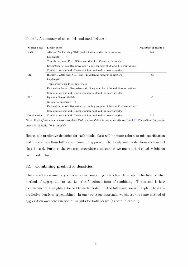
Table 1. A summary of all models and model classes
Model class Description Number of models
VAR ARs and VARs using GDP (and inflation and/or interest rate) 144
Lag length: 1− 4
Transformations: First differences, double differences, detrended
Estimation period: Recursive and rolling samples of 20 and 30 observations
Combination method: Linear opinion pool and log score weights
LIM Bivariate VARs with GDP and 120 different monthly indicators 360
Lag-length: 1
Transformations: First differences
Estimation Period: Recursive and rolling samples of 20 and 30 observations
Combination method: Linear opinion pool and log score weights
FM Dynamic Factor Models 12
Number of factors: 1− 4
Estimation period: Recursive and rolling samples of 20 and 30 observations
Combination method: Linear opinion pool and log score weights
Combination Combination method: Linear opinion pool and log score weights 516
Note: Each of the model classes are described in more detail in the appendix section 7.2. The estimation period
starts in 1982M1 for all models.
Hence, our predictive densities for each model class will be more robust to mis-specification
and instabilities than following a common approach where only one model from each model
class is used. Further, the two-step procedure ensures that we put a priori equal weight on
each model class.
3.1 Combining predictive densities
There are two elementary choices when combining predictive densities. The first is what
method of aggregation to use, i.e. the functional form of combining. The second is how
to construct the weights attached to each model. In the following, we will explain how the
predictive densities are combined. In our two-stage approach, we choose the same method of
aggregation and construction of weights for both stages (as seen in table 1).
7

3.1.1 Method of aggregation
One popular approach to solve the aggregation problem is to take a linear combination of the
individual density forecasts, the so called linear opinion pool:
p(yτ,h) =N∑i=1
wi,τ,h g(yτ,h|Ii,τ ), τ = τ , ..., τ (1)
where N denotes the number of models to combine, Ii,τ is the information set used by model
i to produce the density forecast g(yτ,h|Ii,τ ) for variable y at forecasting horizon h. τ and τ
are the period over which the individual forecasters’ densities are evaluated, and finally wi,τ,h
are a set of non-negative weights that sum to unity (see section 3.1.2).
Combining the N density forecasts according to equation 1 can potentially produce a
combined density forecast with characteristics quite different from those of the individual
forecasters. As Hall and Mitchell (2007) notes; if all the individual forecasters’ densities are
normal, but with different mean and variance, the combined density forecast using the linear
opinion pool will be mixture normal. This distribution can accommodate both skewness and
kurtosis and be multimodal, see Kascha and Ravazzolo (2010).11 If the true unknown density
is non-normal, this is a appealing feature.
3.1.2 Deriving the weights
Many different weighting schemes have been proposed in the literature. Equally-weighted
combinations have been found to be surprisingly effective for point forecasting, see Clemen
(1989) and Stock and Watson (2004). Bates and Granger (1969) propose another alternative,
combining models using weights derived from their sum of squared errors (SSE). These weights
will minimise a quadratic loss function based on forecast errors, provided that the estimation
errors of different models are uncorrelated. Using inverse-SSE weights produces the same
weights as those derived from the inverse of mean squared errors (MSEs) computed over
some recent observed sample:
wi,τ,h =
1MSEi,τ,h∑Ni=1
1MSEi,τ,h
, τ = τ , ..., τ (2)
11Further, since the combined density is a linear combination of all the individual forecasters’ densities, the
variance of the combined density forecast will in general, and more realistic, be higher than that of individual
models. The reason is that the variance of the combination is equal to the weighted sum of a measure of model
uncertainty and dispersion (or disagreement) of the point forecast, see Wallis (2005).
8
where τ, h,N and i are defined above.
In a density combination setting, the range of possible weighting schemes is richer. It is
possible to calculate MSEs based on the means of the distributions, but it is more natural to
take advantage of the full distributions, see e.g. Jore et al. (2010) and Amisano and Geweke
(2009). Then the question of evaluating densities arises.
A popular statistical measure is the Kullback-Leibler divergence or Kullback-Leibler in-
formation criterion (KLIC), see Mitchell and Hall (2005), Amisano and Giacomini (2007) and
Kascha and Ravazzolo (2010). The KLIC is a sensible measure of accuracy since it chooses
the model which on average gives higher probability to events that have actually occurred.
As argued by Mitchell and Hall (2005) the KLIC provides a unified framework for evaluating,
comparing and combining density forecasts, and Mitchell and Wallis (2010) show that the
KLIC can be interpreted as a mean error, similar to the use of the mean error or bias in point
forecast evaluation.12 Specifically, the KLIC distance between the true density f of a random
variable yt and some candidate density fi(yt) obtained from the individual model i is defined
as
KLICi =
∫ft(yt) ln
f(yt)
fi(yt)dyt = E[ln f(yt)− ln fi(yt)], (3)
where E denotes the expectation. The KLIC difference between two densities is then
defined as
KLICi −KLICj = E[ln f(yt)− ln fi(yt)]− E[ln f(yt)− ln fj(yt)]
= E[ln fj(yt)]− E[ln fi(yt)]
= E lnSj − E lnSi, (4)
i.e. the difference between two expected log scores. Thus, when E lnSj > E lnSi, then
KLICj < KLICi. Under some regularity conditions, ElnSi can be estimated by the average
log score
lnSi =1
T
T∑t=1
ln fi(yt). (5)
It follows from equation 4 that we do not need to know the true density in order to
compare two candidate densities. When comparing density forecasts, a measure of out-of-
12As discussed in Hoeting et al. (1999), the log score is a combined measure of bias and calibration.
9
sample performance is the (out-of-sample) log score given by
lnSi,h =1
T − h− TS + 1
T−h∑t=TS
ln ft+h,t,i(yt+h), (6)
where ft+h,t,i denotes a prediction of the density for Yt+h conditional on some information set
available at time t, and TS and T denotes respectively the starting period for the forecasts
and number of observations.
Hence, the log score is the logarithm of the probability density function evaluated at the
outturn of the forecast. Following Jore et al. (2010) we define the recursive log score weights
as:
wi,τ,h =exp[
∑τ−hτ ln f(yτ,h|Ii,τ )]∑N
i=1 exp[∑τ−h
τ ln f(yτ,h|Ii,τ )]=
lnSi,τ,h∑Ni=1 lnSi,τ,h
, τ = τ , ..., τ (7)
where τ, h, y,N, i and g(yτ,h|Ii,τ ) are defined above. Two points are worth emphasizing about
this expression. The weights are derived based on out-of-sample performance, and the weights
are horizon specific.
3.2 Evaluating density forecasts
Corradi and Swanson (2006) provide an extensive survey of the theoretical literature on
density evaluation. In general, the literature is divided in two branches. One branch is
concerned with scoring rules and distance measures, where scoring rules evaluate the quality of
probability forecasts by assigning a numerical score based on the forecast and the subsequent
realization of the variable, see section 3.1.2.
Another common approach for evaluating density forecasts provides statistics suitable for
test of forecast accuracy relative to the “true” unobserved density. Following Rosenblatt
(1952), Dawid (1984) and Diebold et al. (1998), we evaluate the density relative to the “true”
but unobserved density using the probability integral transform (pits). The pits summarize
the properties of the densities, and may help us to judge whether the densities are biased in a
particular direction, and whether the width of the densities have been roughly correct on av-
erage. More precisely, the pits represent the ex-ante inverse predictive cumulative distribution
evaluated at the ex-post actual observations.
10

A density is correctly specified if the pits are uniform, identically and, for one-step ahead
forecasts, independently distributed. Accordingly, we may test for uniformity and indepen-
dence at the end of the evaluation period. Several candidate tests exists, but few offer a
composite test of uniformity and independence together, as would be appropriate for one-
step ahead forecasts. In general, tests for uniformity are not independent of possible depen-
dence and vice versa. Since the appropriateness of the tests are uncertain, we conduct several
different tests. See Hall and Mitchell (2007) for elaboration and description of different tests.
We use a test of uniformity of the pits proposed by Berkowitz (2001). The Berkowitz
test works with the inverse normal cumulative density function transformation of the pits.
Then we can test for normality instead of uniformity. For 1-step ahead forecasts, the null
hypothesis is that the transformed pits are identically and independently normally distributed,
iid N(0,1). The test statistics is χ2 with three degrees of freedom. For longer horizons, we
do not test for independence. In these cases, the null hypothesis is that the transformed
pits are identically, normally distributed, N(0,1). The test statistics is χ2 with two degrees
of freedom. Other tests of uniformity are the Anderson-Darling (AD) test (see Noceti et al.
(2003)) and a Pearson chi-squared test suggested by Wallis (2003). Note that the two latter
tests are more suitable for small-samples. Independence of the pits is tested by a Ljung-Box
test, based on autocorrelation coefficients up to four for one-step ahead forecasts. For forecast
horizons h>1, we test for autocorrelation at lags equal to or greater than h.
4 Empirical exercise and ordering of data blocks
Our recursive forecasting exercise is intended to mimic the behavior of a policymaker now-
casting in real-time. We use real-time data vintages for the U.S. economy for all forecasts
and realizations (see section 2 for details). A key issue in this exercise is the choice of bench-
mark representing the “actual” measure of GDP. Stark and Croushore (2002) suggest three
alternative benchmark data vintages: the most recent data vintage, the last vintage before a
structural revision (called benchmark vintages) and finally the vintage that is released a fixed
period of time after the first release. We follow Clark and McCracken (2010) and Jore et al.
(2010) and use the second available estimate of GDP as actual.13
13Our results are highly robust to using the fifth and the last vintage of GDP as actuals, see section 5.3.3
for more details.
11
We perform a real-time out-of-sample density nowcasting exercise for quarterly U.S. GDP
growth. The recursive forecast exercise is constructed as follows: We estimate each model
on a real-time sample and compute model nowcast/backcast for GDP. For each vintage of
GDP we re-estimate all models and compute predictive densities (for all individual models,
model classes and the combination) for every new data release within the quarter of interest
(nowcast) until the first estimate of GDP is released. This will be approximately 3 weeks
after the end of the quarter. By then the nowcast has turned into a backcast for that quarter.
The data we consider are either of monthly or quarterly frequency. Data series that have
similar release dates and are similar in content are grouped together in blocks. Hence, some
blocks of data will be updated every month, while others are only updated once every quarter.
In total we have defined 15 different blocks, where the number of variables in each block varies
from 30 in “Labor Market” to only 2 in “Money & Credit”.14
In Table 2, we illustrate the data release calender and depict how the 15 different blocks
are released throughout any month and quarter until the first release of GDP is available. The
table shows for each model class the number of individual models that update their nowcast
after every new data release. It also illustrates if the GDP nowcast is a two-step ahead or a
one-step ahead forecast. Note that since all the individual models in the VAR class are of
quarterly frequency, their nowcasts only change three times per quarter. That is whenever a
full quarter of CPI inflation, interest rates or GDP is available. Nowcasts from the leading
indicator model (LIM) class and the factor model (FM) class are, on the other hand, updated
for every single new data release. However, while nowcasts from all the 12 factor models are
updated for every new data release, only nowcasts from a fraction of the leading indicator
models are updated. That is, only models that include the newly released data will update
their nowcasts. This illustrates a key difference between how the density nowcasts from the
FM class and the LIM class are revised. Where the nowcast from the FM class changes
for every data release (since the factors are affected), the nowcast from the LIM class only
changes if the newly released data contains information that historically has improved the log
score. That is, if the models that revise their nowcast have a non-zero weight.
Finally, note that release lags vary for the different data series, ranging from 2 months for
14On some dates more than one block is released, however our results are robust to alternative ordering of
the blocks.
12

Table 2. Structure of data releases and models updated from the start of the quarter until the
first estimate of GDP is released.Number of models updated
Release Block Time Horizon VAR Indicator Factor Combination
Now
cast
1 Interest rate January 2 72 9 12 932 Financials 2 36 12 483 Surveys 2 2 18 12 304 Labor market 2 90 12 1025 Money & Credit 2 6 12 186 Mixed 1 2 15 12 277 Ind. Production 2 48 12 608 Mixed 2 2 33 12 459 PPI 2 21 12 3310 CPI 2 72 39 12 12311 GDP 1 144 360 12 51612 GDP & Income 1 21 12 3313 Housing 1 9 12 2114 Survey 1 1 12 12 2415 Initial Claims 1 3 12 15
16 Interest rate February 1 9 12 2117 Financials 1 36 12 4818 Surveys 2 1 18 12 3019 Labor market 1 90 12 10220 Money & Credit 1 6 12 1821 Mixed 1 1 15 12 2722 Ind. Production 1 48 12 6023 Mixed 2 1 33 12 4524 PPI 1 21 12 3325 CPI 1 39 12 5126 GDP 127 GDP & Income 1 21 12 3328 Housing 1 9 12 2129 Survey 1 1 12 12 2430 Initial Claims 1 3 12 15
31 Interest rate March 1 9 12 2132 Financials 1 36 12 4833 Surveys 2 1 18 12 3034 Labor market 1 90 12 10235 Money & Credit 1 6 12 1836 Mixed 1 1 15 12 2737 Ind. Production 1 48 12 6038 Mixed 2 1 33 12 4539 PPI 1 21 12 3340 CPI 1 39 12 5141 GDP 142 GDP & Income 1 21 12 3343 Housing 1 9 12 2144 Survey 1 1 12 12 2445 Initial Claims 1 3 12 15
Backcast
46 Interest rate April 1 72 9 12 9347 Financials 1 36 12 4848 Surveys 2 1 18 12 3049 Labor market 1 90 12 10250 Money & Credit 1 6 12 1851 Mixed 1 1 15 12 2752 Ind. Production 1 48 12 6053 Mixed 2 1 33 12 4554 PPI 1 21 12 3355 CPI 1 72 39 12 12356 GDP 1 144 360 12 516
Note: The table illustrates a generic quarter of our real-time out of sample forecasting experiment. Our forecast
evaluation period runs from 1990Q2 to 2010Q3, which gives us more than 80 observations to evaluate for each
data release. All models that are updated are re-estimated at each point in time throughout the quarter. In
total we re-estimate and simulate the individual models well over 3000 times during a given quarter.
imports and exports data to current month for Business outlook surveys. Thus, the structure
of the unbalancedness changes when a new block is released.
13
5 Results
In this section, we analyze the performance of our two-stage density nowcast combination
approach. The main goal of our exercise is to study how the predictive densities improve as
more data are available throughout the quarter. In doing so, we want to evaluate both the
accuracy of the density nowcasts, section 5.1, and if they are well-calibrated, section 5.2.
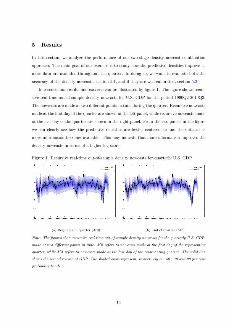
In essence, our results and exercise can be illustrated by figure 1. The figure shows recur-
sive real-time out-of-sample density nowcasts for U.S. GDP for the period 1990Q2-2010Q3.
The nowcasts are made at two different points in time during the quarter. Recursive nowcasts
made at the first day of the quarter are shown in the left panel, while recursive nowcasts made
at the last day of the quarter are shown in the right panel. From the two panels in the figure
we can clearly see how the predictive densities are better centered around the outturn as
more information becomes available. This may indicate that more information improves the
density nowcasts in terms of a higher log score.
Figure 1. Recursive real-time out-of-sample density nowcasts for quarterly U.S. GDP
(a) Beginning of quarter (M0) (b) End of quarter (M3)
Note: The figures show recursive real-time out-of-sample density nowcasts for the quarterly U.S. GDP,
made at two different points in time. M0 refers to nowcasts made at the first day of the representing
quarter, while M3 refers to nowcasts made at the last day of the representing quarter. The solid line
shows the second release of GDP. The shaded areas represent, respectively 30, 50 , 70 and 90 per cent
probability bands.
14

Figure 2. Average log scores for forecasts after different block releases. Evaluated against 2nd
release of data
−1.3
−1.2
−1.1
−1
−0.9
−0.8
−0.7
−0.6
−0.5
−0.4
Inte
rest
Rat
es
Fin
anci
al
Sur
veys
2
Labo
r &
Wag
es
Mon
ey &
Cre
dit
Mix
ed 1
In
d.P
rodu
ctio
n M
ixed
2
PP
I C
PI
GD
P
GD
P &
Inco
me
Hou
sing
S
urve
ys 1
In
itial
Cla
ims
Inte
rest
Rat
es
Fin
anci
al
Sur
veys
2
Labo
r &
Wag
es
Mon
ey &
Cre
dit
Mix
ed 1
In
d.P
rodu
ctio
n M
ixed
2
PP
I C
PI
GD
P &
Inco
me
Hou
sing
S
urve
ys 1
In
itial
Cla
ims
Inte
rest
Rat
es
Fin
anci
al
Sur
veys
2
Labo
r &
Wag
es
Mon
ey &
Cre
dit
Mix
ed 1
In
d.P
rodu
ctio
n M
ixed
2
PP
I C
PI
GD
P &
Inco
me
Hou
sing
S
urve
ys 1
In
itial
Cla
ims
Inte
rest
Rat
es
Fin
anci
al
Sur
veys
2
Labo
r &
Wag
es
Mon
ey &
Cre
dit
Mix
ed 1
In
d.P
rodu
ctio
n M
ixed
2
PP
I C
PI
Inte
rest
Rat
es
Fin
anci
al
Sur
veys
2
Labo
r &
Wag
es
Mon
ey &
Cre
dit
Mix
ed 1
In
d.P
rodu
ctio
n M
ixed
2
PP
I C
PI
GD
P
GD
P &
Inco
me
Hou
sing
S
urve
ys 1
In
itial
Cla
ims
Inte
rest
Rat
es
Fin
anci
al
Sur
veys
2
Labo
r &
Wag
es
Mon
ey &
Cre
dit
Mix
ed 1
In
d.P
rodu
ctio
n M
ixed
2
PP
I C
PI
GD
P &
Inco
me
Hou
sing
S
urve
ys 1
In
itial
Cla
ims
Inte
rest
Rat
es
Fin
anci
al
Sur
veys
2
Labo
r &
Wag
es
Mon
ey &
Cre
dit
Mix
ed 1
In
d.P
rodu
ctio
n M
ixed
2
PP
I C
PI
GD
P &
Inco
me
Hou
sing
S
urve
ys 1
In
itial
Cla
ims
Inte
rest
Rat
es
Fin
anci
al
Sur
veys
2
Labo
r &
Wag
es
Mon
ey &
Cre
dit
Mix
ed 1
In
d.P
rodu
ctio
n M
ixed
2
PP
I C
PI
Nowcasting YFN for US. Average logaritmic score for model classes and combination adding different blocks of information
FMIndicatorVARCombination
Month 1 Month 2 Month 3 Month 4
Note: The individual models within each model class and the model classes have been combined using
the linear opinion pool and log score weights. The evaluation period runs from 1990Q2 to 2010Q3.
5.1 Log score performance
We study the impact of different data releases on the density nowcasting/backcasting pre-
cision, measured by the average log score. Figure 2 depicts the average log scores for the
nowcasts from the combined model and the three model classes after every data block release
over the evaluation period. The 10 first observations of the quarter are actually two step
ahead forecasts, while the 11 last observations are essentially backcasts, see table 2.
The figure reveals two interesting results. First, the forecasting performance improves
when new information becomes available. The log score of the predictive densities for the
model combination and all three model classes increases as new information arrives during
the quarter. Second, the ranking of the model classes changes during the quarter and in
15
accordance with new data releases, while the model combination is always performing well.
In fact, the average log score from the model combination is almost identical to the best
performing model class throughout the quarter. The latter illustrates the main advantage of
using forecast combinations. These results are remarkable robust to choice of “actual” GDP.
While the performance of the different model classes and what data releases that improve
the nowcast the most varies depending on the choice of benchmark (real-time vintage), the
forecast combination is always performing very well. See section 5.3 for more on this.
It is also worth noting that the LIM class and FM class are outperforming the VARs.
This is clearly a result of their informational advantage, as the VARs only utilize quarterly
data. Only immediately after GDP is released, the VARs perform on a par with the FM class.
As new information arrives throughout the quarter, the leading indicator and factor models
adapt faster than the VARs. This highlights the importance of utilizing higher frequency and
non-synchronous data releases for nowcasting. Finally, figure 8 in the appendix shows in more
detail how the different data releases improve the combined nowcasts as well as the nowcasts
from the three model classes. The blocks of data that improves the nowcasts the most are
“Ind. Production” and “Initial Claims”.
In figure 3, we depict the weights attached to each model class in the combined density
forecast after every data block release. The figure illustrates the time-varying weights at the
end of the evaluation period. As we would expect from figure 2 there are large changes in
the weights throughout the quarter. The LIM class has a high weight in the early periods
of the quarter, while the FM class gets higher weight as we move further into the quarter.15
Towards the end of the quarter, the factor models ends up having almost all the weight. The
reader should however not interpret this as attaching all weight to one unique model, as the
FM class is a combination of 12 factor models. The VAR models seem to get very little
weight throughout the quarter. Again, this must be seen as a result of their informational
disadvantage relative to the factor models and leading indicator models.
15Note, that labor market data tends to increase the weight attached to the FM class, while GDP releases
seem to increase the weight attached to the LIM class.
16

Figure 3. End of sample weights attached to the different model classes after different block
releases. Evaluated against 2nd release of data
0
0.1
0.2
0.3
0.4
0.5
0.6
0.7
0.8
0.9
1
Inte
rest
Rat
es
Fin
anci
al
Sur
veys
2
Labo
r &
Wag
es
Mon
ey &
Cre
dit
Mix
ed 1
In
d.P
rodu
ctio
n M
ixed
2
PP
I C
PI
GD
P
GD
P &
Inco
me
Hou
sing
S
urve
ys 1
In
itial
Cla
ims
Inte
rest
Rat
es
Fin
anci
al
Sur
veys
2
Labo
r &
Wag
es
Mon
ey &
Cre
dit
Mix
ed 1
In
d.P
rodu
ctio
n M
ixed
2
PP
I C
PI
GD
P &
Inco
me
Hou
sing
S
urve
ys 1
In
itial
Cla
ims
Inte
rest
Rat
es
Fin
anci
al
Sur
veys
2
Labo
r &
Wag
es
Mon
ey &
Cre
dit
Mix
ed 1
In
d.P
rodu
ctio
n M
ixed
2
PP
I C
PI
GD
P &
Inco
me
Hou
sing
S
urve
ys 1
In
itial
Cla
ims
Inte
rest
Rat
es
Fin
anci
al
Sur
veys
2
Labo
r &
Wag
es
Mon
ey &
Cre
dit
Mix
ed 1
In
d.P
rodu
ctio
n M
ixed
2
PP
I C
PI
Inte
rest
Rat
es
Fin
anci
al
Sur
veys
2
Labo
r &
Wag
es
Mon
ey &
Cre
dit
Mix
ed 1
In
d.P
rodu
ctio
n M
ixed
2
PP
I C
PI
GD
P
GD
P &
Inco
me
Hou
sing
S
urve
ys 1
In
itial
Cla
ims
Inte
rest
Rat
es
Fin
anci
al
Sur
veys
2
Labo
r &
Wag
es
Mon
ey &
Cre
dit
Mix
ed 1
In
d.P
rodu
ctio
n M
ixed
2
PP
I C
PI
GD
P &
Inco
me
Hou
sing
S
urve
ys 1
In
itial
Cla
ims
Inte
rest
Rat
es
Fin
anci
al
Sur
veys
2
Labo
r &
Wag
es
Mon
ey &
Cre
dit
Mix
ed 1
In
d.P
rodu
ctio
n M
ixed
2
PP
I C
PI
GD
P &
Inco
me
Hou
sing
S
urve
ys 1
In
itial
Cla
ims
Inte
rest
Rat
es
Fin
anci
al
Sur
veys
2
Labo
r &
Wag
es
Mon
ey &
Cre
dit
Mix
ed 1
In
d.P
rodu
ctio
n M
ixed
2
PP
I C
PI
Nowcasting YFN for US. Weights for model classes in combination when adding different blocks of information
FMIndicatorVAR
Note: The individual models within each model class and the model classes have been combined using
the linear opinion pool and log score weights. The evaluation period runs from 1990Q2 to 2010Q3.
5.2 Testing the pits
We evaluate the predictive densities relative to the “true” but unobserved density using the
pits of the realization of the variable with respect to the nowcast densities, see figure 4. Table
3 shows p-values for the four different tests, described in section 3.2, applied to the combined
forecast at five different points in time (M0 −M4).16 P-values equal to or higher than 0.05
mean that we can not reject the hypothesis that the combination is correctly calibrated at a
95% significance level.
The predictive densities of the combined forecast passes all tests for horizon M0. This is
the case where the nowcast corresponds to a two-step ahead forecast. Turning to the one-step
16To save space, we only report test results for the final combined density. More results are available upon
request.
17

Figure 4. Pits of the combined density forecast at five points in the quarter. The pits are the ex
ante inverse predictive cumulative distributions evaluated at the ex post actual observations.
0 0.1 0.2 0.3 0.4 0.5 0.6 0.7 0.8 0.9 10
2
4
6
8
10
12
14
16
18
20PITs
Probability integral transforms
Fre
quen
cy (
# of
obs
erva
tions
)
m0 m1 m2 m3 m4
Note: The pits of predictive densities should have a standard uniform distribution if the model is
correctly specified. The M0 bars refers to the 1th release of a generic quarter (see table 2), while M1,
M2, M3 and M4 refer respectively to release 15, 30, 45 and 57.
ahead forecast (M1 −M4), the predictive densities of the combined forecast also seem to
be well-calibrated. Based on the Berkowitz test, the Anderson-Darling test and the Pearson
chi-squared test, we cannot reject the null hypothesis that the combination is well-calibrated
at a 95% significance level.17
17The null hypothesis in the Ljung-Box test is rejected at horizon M4.
18

Table 3. Pits tests for evaluating density forecasts for GDP (p-values)
LogScore Berkowitz Wallis Ljung-Box Anderson-Darling
m0 nowcast -0.89 0.82 0.27 0.61 0.67
m1 nowcast -0.77 0.65 0.73 0.53 0.46
m2 nowcast -0.69 0.40 0.87 0.30 0.26
m3 nowcast -0.54 0.21 0.76 0.20 0.25
m4 backcast -0.54 0.46 0.30 0.00 0.43
Note: The null hypothesis in the Berkowitz test is that the inverse normal cumulative distribution function
transformed pits are identically, normally distributed, N(0,1), and for h = 1 independent. χ2 is the Pearson
chi-squared test suggested by Wallis (2003) of uniformity of the pits histogram in eigth equiprobable classes.
Ljung-Box is a test for independence of the pits (in the first power) at lags greater than or equal to the horizon.
The Anderson-Darling test is a test for uniformity of the pits, with the small-sample (simulated) p-values
computed assuming independence of the pits.
5.3 Robustness
As already noted, our results are robust to changes in the ordering of data releases.18 In
this section we perform three additional robustness checks: First, with respect to alternative
weighting schemes. Second, with respect to point forecasting. Finally, we check for robustness
with respect to choice of benchmark vintage for GDP.
5.3.1 Alternative weighting schemes for the combination
Several papers have found that simple combination forecasts, as equal weights, outperform
more sophisticated adaptive forecast combination methods. This is often referred to as the
forecast combination puzzle. While Jore et al. (2010) and Gerdrup et al. (2009) seem to find
some evidence of gains from adaptive log score weights for density combination, this is still a
question of debate. We check for robustness with respect to the following different weighting
schemes: 1) combination of all models applying equal weights (Equal) and 2) combination
of all models applying log score weights (LogS) and c) two-stage nowcast combination with
equal weights in both stages (Equal-Equal) and 4) a selection strategy where we try to pick
the “best” model. We have constructed this by recursively “picking” the best model among
all the 516 models at each point in time throughout the evaluation period, and used this
18The results can be given on request.
19

to forecast the next period.19 The preferred two-stage nowcast combination with log score
weights in both stages is denoted as LogS-LogS.
Figure 5. Comparing different weighting schemes. Average log scores for forecasts after
different block releases. Evaluated against 2nd release of data
−1.3
−1.2
−1.1
−1
−0.9
−0.8
−0.7
−0.6
−0.5
−0.4
Inte
rest
Rat
es
Fin
anci
al
Sur
veys
2
Labo
r &
Wag
es
Mon
ey &
Cre
dit
Mix
ed 1
In
d.P
rodu
ctio
n M
ixed
2
PP
I C
PI
GD
P
GD
P &
Inco
me
Hou
sing
S
urve
ys 1
In
itial
Cla
ims
Inte
rest
Rat
es
Fin
anci
al
Sur
veys
2
Labo
r &
Wag
es
Mon
ey &
Cre
dit
Mix
ed 1
In
d.P
rodu
ctio
n M
ixed
2
PP
I C
PI
GD
P &
Inco
me
Hou
sing
S
urve
ys 1
In
itial
Cla
ims
Inte
rest
Rat
es
Fin
anci
al
Sur
veys
2
Labo
r &
Wag
es
Mon
ey &
Cre
dit
Mix
ed 1
In
d.P
rodu
ctio
n M
ixed
2
PP
I C
PI
GD
P &
Inco
me
Hou
sing
S
urve
ys 1
In
itial
Cla
ims
Inte
rest
Rat
es
Fin
anci
al
Sur
veys
2
Labo
r &
Wag
es
Mon
ey &
Cre
dit
Mix
ed 1
In
d.P
rodu
ctio
n M
ixed
2
PP
I C
PI
Inte
rest
Rat
es
Fin
anci
al
Sur
veys
2
Labo
r &
Wag
es
Mon
ey &
Cre
dit
Mix
ed 1
In
d.P
rodu
ctio
n M
ixed
2
PP
I C
PI
GD
P
GD
P &
Inco
me
Hou
sing
S
urve
ys 1
In
itial
Cla
ims
Inte
rest
Rat
es
Fin
anci
al
Sur
veys
2
Labo
r &
Wag
es
Mon
ey &
Cre
dit
Mix
ed 1
In
d.P
rodu
ctio
n M
ixed
2
PP
I C
PI
GD
P &
Inco
me
Hou
sing
S
urve
ys 1
In
itial
Cla
ims
Inte
rest
Rat
es
Fin
anci
al
Sur
veys
2
Labo
r &
Wag
es
Mon
ey &
Cre
dit
Mix
ed 1
In
d.P
rodu
ctio
n M
ixed
2
PP
I C
PI
GD
P &
Inco
me
Hou
sing
S
urve
ys 1
In
itial
Cla
ims
Inte
rest
Rat
es
Fin
anci
al
Sur
veys
2
Labo
r &
Wag
es
Mon
ey &
Cre
dit
Mix
ed 1
In
d.P
rodu
ctio
n M
ixed
2
PP
I C
PI
Inte
rest
Rat
es
Fin
anci
al
Sur
veys
2
Labo
r &
Wag
es
Mon
ey &
Cre
dit
Mix
ed 1
In
d.P
rodu
ctio
n M
ixed
2
PP
I C
PI
GD
P
GD
P &
Inco
me
Hou
sing
S
urve
ys 1
In
itial
Cla
ims
Inte
rest
Rat
es
Fin
anci
al
Sur
veys
2
Labo
r &
Wag
es
Mon
ey &
Cre
dit
Mix
ed 1
In
d.P
rodu
ctio
n M
ixed
2
PP
I C
PI
GD
P &
Inco
me
Hou
sing
S
urve
ys 1
In
itial
Cla
ims
Inte
rest
Rat
es
Fin
anci
al
Sur
veys
2
Labo
r &
Wag
es
Mon
ey &
Cre
dit
Mix
ed 1
In
d.P
rodu
ctio
n M
ixed
2
PP
I C
PI
GD
P &
Inco
me
Hou
sing
S
urve
ys 1
In
itial
Cla
ims
Inte
rest
Rat
es
Fin
anci
al
Sur
veys
2
Labo
r &
Wag
es
Mon
ey &
Cre
dit
Mix
ed 1
In
d.P
rodu
ctio
n M
ixed
2
PP
I C
PI
Inte
rest
Rat
es
Fin
anci
al
Sur
veys
2
Labo
r &
Wag
es
Mon
ey &
Cre
dit
Mix
ed 1
In
d.P
rodu
ctio
n M
ixed
2
PP
I C
PI
GD
P
GD
P &
Inco
me
Hou
sing
S
urve
ys 1
In
itial
Cla
ims
Inte
rest
Rat
es
Fin
anci
al
Sur
veys
2
Labo
r &
Wag
es
Mon
ey &
Cre
dit
Mix
ed 1
In
d.P
rodu
ctio
n M
ixed
2
PP
I C
PI
GD
P &
Inco
me
Hou
sing
S
urve
ys 1
In
itial
Cla
ims
Inte
rest
Rat
es
Fin
anci
al
Sur
veys
2
Labo
r &
Wag
es
Mon
ey &
Cre
dit
Mix
ed 1
In
d.P
rodu
ctio
n M
ixed
2
PP
I C
PI
GD
P &
Inco
me
Hou
sing
S
urve
ys 1
In
itial
Cla
ims
Inte
rest
Rat
es
Fin
anci
al
Sur
veys
2
Labo
r &
Wag
es
Mon
ey &
Cre
dit
Mix
ed 1
In
d.P
rodu
ctio
n M
ixed
2
PP
I C
PI
Inte
rest
Rat
es
Fin
anci
al
Sur
veys
2
Labo
r &
Wag
es
Mon
ey &
Cre
dit
Mix
ed 1
In
d.P
rodu
ctio
n M
ixed
2
PP
I C
PI
GD
P
GD
P &
Inco
me
Hou
sing
S
urve
ys 1
In
itial
Cla
ims
Inte
rest
Rat
es
Fin
anci
al
Sur
veys
2
Labo
r &
Wag
es
Mon
ey &
Cre
dit
Mix
ed 1
In
d.P
rodu
ctio
n M
ixed
2
PP
I C
PI
GD
P &
Inco
me
Hou
sing
S
urve
ys 1
In
itial
Cla
ims
Inte
rest
Rat
es
Fin
anci
al
Sur
veys
2
Labo
r &
Wag
es
Mon
ey &
Cre
dit
Mix
ed 1
In
d.P
rodu
ctio
n M
ixed
2
PP
I C
PI
GD
P &
Inco
me
Hou
sing
S
urve
ys 1
In
itial
Cla
ims
Inte
rest
Rat
es
Fin
anci
al
Sur
veys
2
Labo
r &
Wag
es
Mon
ey &
Cre
dit
Mix
ed 1
In
d.P
rodu
ctio
n M
ixed
2
PP
I C
PI
Nowcasting YFN for US. Average logaritmic score for model classes and combination adding different blocks of information
EqualLogSEqual−EqualLogS−LogSSelection
Month 1 Month 2 Month 3 Month 4
Note: Equal and LogS denote that all individual models are combined using linear opinion pool and
respectively equal weights or log score weights. Equal-Equal and LogS-LogS denotes that the individual
models within each model class and the combination have been combined using the linear opinion pool
and respectively equal weights and log score weights. Selection refers to a strategy of “picking” the best
model among all the 516 models at each point in time throughout the evaluation period. The evaluation
period runs from 1990Q2 to 2010Q3.
19In practice this is often the strategy that is employed when model combination is not conducted. As new
models are tested and developed, they outstrip and replace the older models as time goes by. Our baseline
real-time model combination experiment tries to be as honest as possible in this respect, by not replacing any
of the 516 individual models during the evaluation period. However, the selection strategy we test is of course
rather extreme, as we for each new data release and quarter do a selection based on the historical performance
up to that point in time.
20

Figure 5 compares the average log score for the different weighting schemes. There are five
interesting results. First, all combination methods yield a steady increase in the average log
score as more information becomes available. This is not the case for the selection strategy,
which gives large and volatile changes in the average log score after every data block release.
Second, the selection strategy seems to almost always give the poorest density nowcast in
terms of having the lowest average log score. Third, the difference between “Equal” an
“Equal-Equal” can be seen as the “pure” gain from using a two-stage approach where models
are first grouped into model classes and then combined together. It is evident from the
figure that “Equal-Equal” is always performing better than “Equal”. Fourth, there is less
differences between the “LogS” and “LogS-LogS”, as the log score weights discriminate rather
sharply between nowcasts from the different models. Finally, no weighting scheme is superior
throughout the quarter, but our preferred two-stage combination approach (“LogS-LogS”) is
the best performing strategy for most of the quarter.
5.3.2 Point forecasting
Although the main purpose of this paper is to evaluate density nowcasts, we do check for
robustness of our results with respect to point nowcasting performance. We do this by com-
paring three different combination strategies. In the first strategy we follow the two stage
density combination strategy explained above, but calculate the final point nowcasts as the
center of the final combined density nowcast. In the second strategy we calculate the point
nowcasts for each single model as the center of the predictive density already before we com-
bine the models in the first stage. We then use inverse mean squared errors (MSE) to calculate
weights between the models within each model class, as well as between the three different
model classes, see section 3.1.2. Finally, we calculate final point nowcast using a strategy
where we apply equal weigths to all models in both stages. For all three strategies we evalu-
ate the final point forecasts using the root mean squared prediction error (RMSE). The rest
of the experiment is similar to what is explained earlier.
Figure 6 depicts the RMSE for the combined nowcasts from the three strategies after
every data block release. The figure displays two interesting results.
First, for all strategies the nowcasting errors are steadily reduced as more information
becomes available throughout the quarter and until the first estimate of GDP is released.
21
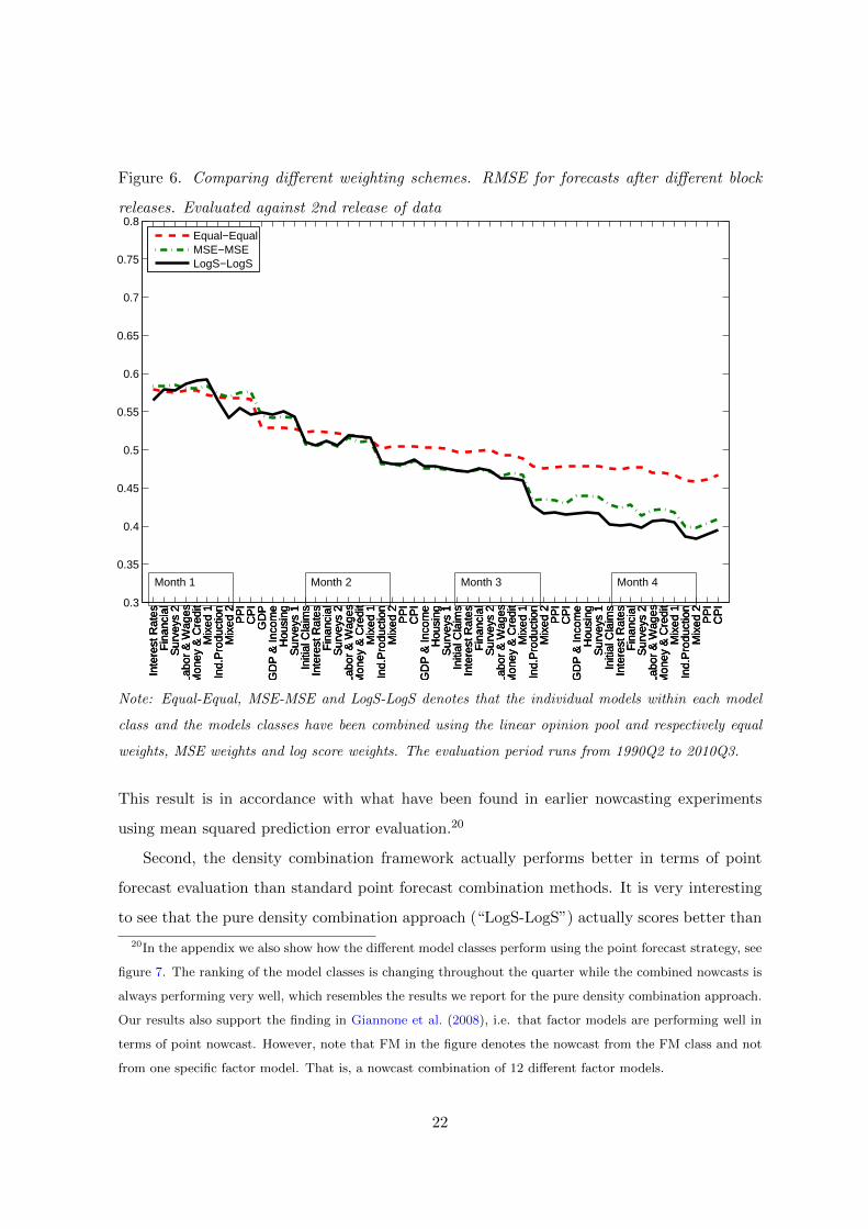
Figure 6. Comparing different weighting schemes. RMSE for forecasts after different block
releases. Evaluated against 2nd release of data
0.3
0.35
0.4
0.45
0.5
0.55
0.6
0.65
0.7
0.75
0.8
Inte
rest
Rat
es
Fin
anci
al
Sur
veys
2
Labo
r &
Wag
es
Mon
ey &
Cre
dit
Mix
ed 1
In
d.P
rodu
ctio
n M
ixed
2
PP
I C
PI
GD
P
GD
P &
Inco
me
Hou
sing
S
urve
ys 1
In
itial
Cla
ims
Inte
rest
Rat
es
Fin
anci
al
Sur
veys
2
Labo
r &
Wag
es
Mon
ey &
Cre
dit
Mix
ed 1
In
d.P
rodu
ctio
n M
ixed
2
PP
I C
PI
GD
P &
Inco
me
Hou
sing
S
urve
ys 1
In
itial
Cla
ims
Inte
rest
Rat
es
Fin
anci
al
Sur
veys
2
Labo
r &
Wag
es
Mon
ey &
Cre
dit
Mix
ed 1
In
d.P
rodu
ctio
n M
ixed
2
PP
I C
PI
GD
P &
Inco
me
Hou
sing
S
urve
ys 1
In
itial
Cla
ims
Inte
rest
Rat
es
Fin
anci
al
Sur
veys
2
Labo
r &
Wag
es
Mon
ey &
Cre
dit
Mix
ed 1
In
d.P
rodu
ctio
n M
ixed
2
PP
I C
PI
Inte
rest
Rat
es
Fin
anci
al
Sur
veys
2
Labo
r &
Wag
es
Mon
ey &
Cre
dit
Mix
ed 1
In
d.P
rodu
ctio
n M
ixed
2
PP
I C
PI
GD
P
GD
P &
Inco
me
Hou
sing
S
urve
ys 1
In
itial
Cla
ims
Inte
rest
Rat
es
Fin
anci
al
Sur
veys
2
Labo
r &
Wag
es
Mon
ey &
Cre
dit
Mix
ed 1
In
d.P
rodu
ctio
n M
ixed
2
PP
I C
PI
GD
P &
Inco
me
Hou
sing
S
urve
ys 1
In
itial
Cla
ims
Inte
rest
Rat
es
Fin
anci
al
Sur
veys
2
Labo
r &
Wag
es
Mon
ey &
Cre
dit
Mix
ed 1
In
d.P
rodu
ctio
n M
ixed
2
PP
I C
PI
GD
P &
Inco
me
Hou
sing
S
urve
ys 1
In
itial
Cla
ims
Inte
rest
Rat
es
Fin
anci
al
Sur
veys
2
Labo
r &
Wag
es
Mon
ey &
Cre
dit
Mix
ed 1
In
d.P
rodu
ctio
n M
ixed
2
PP
I C
PI
Nowcasting YFN for US. Average logaritmic score for model classes and combination adding different blocks of information
Equal−EqualMSE−MSELogS−LogS
Month 1 Month 2 Month 3 Month 4
Note: Equal-Equal, MSE-MSE and LogS-LogS denotes that the individual models within each model
class and the models classes have been combined using the linear opinion pool and respectively equal
weights, MSE weights and log score weights. The evaluation period runs from 1990Q2 to 2010Q3.
This result is in accordance with what have been found in earlier nowcasting experiments
using mean squared prediction error evaluation.20
Second, the density combination framework actually performs better in terms of point
forecast evaluation than standard point forecast combination methods. It is very interesting
to see that the pure density combination approach (“LogS-LogS”) actually scores better than
20In the appendix we also show how the different model classes perform using the point forecast strategy, see
figure 7. The ranking of the model classes is changing throughout the quarter while the combined nowcasts is
always performing very well, which resembles the results we report for the pure density combination approach.
Our results also support the finding in Giannone et al. (2008), i.e. that factor models are performing well in
terms of point nowcast. However, note that FM in the figure denotes the nowcast from the FM class and not
from one specific factor model. That is, a nowcast combination of 12 different factor models.
22

the MSE strategy also in terms of MSE. As far as we are aware of, this is a new finding in the
nowcasting literature. We think the result is linked to the properties of the log score weights.
As new information arrives throughout the quarter, the log score weights adapt faster than
standard point forecast weights (e.g. MSE weights). In this way, our combination procedure
attaches a higher weight to models with new and relevant information. This finding motivates
the potential leverage of density evaluation over simple point forecast evaluation when the
goal is to maximize forecast accuracy in a nowcasting framework.
5.3.3 Alternative benchmark vintages
The choice of benchmark vintage is a key issue in any application using real-time vintage
data.21 In our application, we use the 2nd available vintage of GDP as benchmark. Figure 10
and Figure 11 in the appendix shows results with respectively the 5th release of GDP and the
last available vintage of GDP as benchmark. Clearly the figures show that the nowcasting
performance of the different model classes varies with choice of benchmark vintage. Hence,
also the weights attached to the different model classes varies. However, the result that the
density combination nowcast is always performing well, seems to be remarkably robust. This
implies that there are additional gains from combining forecasts in a real-time environment
where the forecast target (benchmark) is not obvious.
6 Conclusion
In this paper we have used a density combination framework to produce density combination
nowcasts for U.S. quarterly GDP growth from a system of three different model classes widely
used at central banks; VARs, leading indicator models and factor models. The density now-
casts are combined in a two-step procedure. In the first step, we group models into different
model classes. The nowcasts for each model within a model class are combined using the log
score. This yields a combined predictive density nowcast for each of the three different model
classes. In a second step, these three predictive densities are combined into a new density
nowcast using the log score. The density nowcasts are updated for every new data release
during a quarter until the first release of GDP is available. Our recursive nowcasting exercise
21See Croushore (2006) for a survey on forecasting with real-time macroeconomic data.
23

is applied to U.S. real-time data and evaluated on the period 1990Q2-2010Q3.
We show that the log scores for the predictive densities increase almost monotonically as
new information arrives during the quarter. The densities also seem to be well-calibrated.
Further, while the ranking of the model classes is changing during the quarter and in ac-
cordance with new data releases, the model combination is always performing well. Finally,
the density combination approach is superior compared to a simple model selection strategy,
and the density combination framework actually performs better in terms of point forecast
evaluation than standard point forecast combination methods. All our results illustrate the
potential gains from using a density combination approach in a nowcasting environment.
Interestingly these results are very robust to the use of benchmark (real-time) vintage.
While the nowcasting performance from different model classes may vary according to the
benchmark vintage, the density combination nowcast is always performing very well. This
implies that there are additional gains from combining forecasts in a real-time environment
where the forecast target or the benchmark is not obvious.
24
References
Aiolfi, M. and A. Timmermann (2006). Persistence in forecasting performance and conditional
combination strategies. Journal of Econometrics 135 (1-2), 31–53.
Amisano, G. and J. Geweke (2009). Optimal prediction pools. Working Paper Series 1017,
European Central Bank.
Amisano, G. and R. Giacomini (2007). Comparing density foreasts via weighted likelihood
ratio tests. Journal of Business and Economic Statistics 25 (2), 177–190.
Angelini, E., G. Camba-Mendez, D. Giannone, L. Reichlin, and G. Runstler (2011). Short-
term forecasts of euro area gdp growth. Econometrics Journal 14 (1), C25–C44.
Aruoba, S. B., F. X. Diebold, and C. Scotti (2009). Real-time measurement of business
conditions. Journal of Business & Economic Statistics 27 (4), 417–427.
Bache, I. W., A. S. Jore, J. Mitchell, and S. P. Vahey (2011). Combining var and dsge forecast
densities. Journal of Economic Dynamics and Control 35 (10), 1659–1670.
Baffigi, A., R. Golinelli, and G. Parigi (2004). Bridge models to forecast the euro area gdp.
International Journal of Forecasting 20 (3), 447–460.
Banbura, M., D. Giannone, and L. Reichlin (2011). Nowcasting. In M. P. Clements and
D. F. Hendry (Eds.), The Oxford Handbook of Economic Forecasting. Oxford Handbooks
in Economics.
Banerjee, A. and M. Marcellino (2006). Are there any reliable leading indicators for us
inflation and gdp growth? International Journal of Forecasting 22 (1), 137–151.
Banerjee, A., M. Marcellino, and I. Masten (2005). Leading indicators for euro-area inflation
and gdp growth. Oxford Bulletin of Economics and Statistics 67 (s1), 785–813.
Bates, J. and C. Granger (1969). The combination of forecasts. Operations Research Quar-
terly 20 (4), 451–468.
Berkowitz, J. (2001). Testing density forecasts, with applications to risk management. Journal
of Business and Economic Statistics 19 (4), 465–474.
25
Bjørnland, H. C., K. Gerdrup, A. S. Jore, C. Smith, and L. A. Thorsrud (2009). Does
forecast combination improve Norges Bank inflation forecasts? Working Paper 2009/01,
Norges Bank.
Clark, T. E. and M. W. McCracken (2009). Improving forecast accuracy by combining recur-
sive and rolling forecasts. International Economic Review 50 (2), 363–395.
Clark, T. E. and M. W. McCracken (2010). Averaging forecasts from vars with uncertain
instabilities. Journal of Applied Econometrics 25 (1), 5–29.
Clemen, R. T. (1989). Combining forecasts: A review and annotated bibliography. Interna-
tional Journal of Forecasting 5.
Corradi, V. and N. R. Swanson (2006). Predictive Density Evaluation, Volume 1 of Handbook
of Economic Forecasting, Chapter 5, pp. 197–284. Elsevier.
Croushore, D. (2006). Forecasting with Real-Time Macroeconomic Data, Volume 1 of Hand-
book of Economic Forecasting, Chapter 17, pp. 961–982. Elsevier.
Croushore, D. and T. Stark (2001). A real-time data set for macroeconomists. Journal of
Econometrics 105 (1), 111–130.
Dawid, A. P. (1984). Statistical theory: the prequential approach. Journal of the Royal
Statistical Society A 147 (2), 278–290.
Diebold, F. X., T. A. Gunther, and A. S. Tay (1998). Evaluating density forecasts with
applications to financial risk management. International Economic Review 39 (4), 863–83.
Evans, M. D. (2005). Where are we now? real-time estimates of the macro economy. Inter-
national Journal of Central Banking 1 (2), 127–175.
Faust, J. and J. H. Wright (2009). Comparing greenbook and reduced form forecasts using a
large realtime dataset. Journal of Business & Economic Statistics 27 (4), 468–479.
Garratt, A., J. Mitchell, and S. P. Vahey (2009). Measuring output gap uncertainty. Reserve
Bank of New Zealand Discussion Paper Series DP2009/15, Reserve Bank of New Zealand.
Gerdrup, K. R., A. S. Jore, C. Smith, and L. A. Thorsrud (2009). Evaluating ensemble density
combination - forecasting GDP and inflation. Working Paper 2009/19, Norges Bank.
26
Giannone, D., L. Reichlin, and D. Small (2008). Nowcasting: The real-time informational
content of macroeconomic data. Journal of Monetary Economics 55 (4), 665–676.
Gneiting, T. (2011). Making and evaluating point forecasts. Journal of the American Statis-
tical Association 106 (494), 746–762.
Hall, S. G. and J. Mitchell (2007). Combining density forecasts. International Journal of
Forecasting 23 (1), 1–13.
Hoeting, J. A., D. Madigan, A. E. Raftery, and C. T. Volinsky (1999). Bayesian model
averaging: A tutorial. Statistical Science 14 (4), 382–417.
Jore, A. S., J. Mitchell, and S. P. Vahey (2010). Combining forecast densities from vars with
uncertain instabilities. Journal of Applied Econometrics 25 (4), 621–634.
Kascha, C. and F. Ravazzolo (2010). Combining inflation density forecasts. Journal of
Forecasting 29 (1-2), 231–250.
Lutkepohl, H. (2005). New introduction to multiple time series analysis. Springer.
Marcellino, M. (2006). Leading indicators. In G. Elliott, C. W. J. Granger, and A. Tim-
mermann (Eds.), Handbook of Economic Forecasting, Volume 1, pp. 879–960. Amsterdam:
Elsevier.
Mitchell, J. and S. G. Hall (2005). Evaluating, comparing and combining density forecasts
using the klic with an application to the bank of england and niesr ’fan’ charts of inflation.
Oxford Bulletin of Economics and Statistics 67 (s1), 995–1033.
Mitchell, J., G. L. Mazzi, and G. Montana (2010). Density nowcasts and model combination:
nowcasting euro-area gdp growth over the 2008-9 recession. NIESR Discussion Papers 368,
National Institute of Economic and Social Research.
Mitchell, J. and K. Wallis (2010). Evaluating density forecasts: Forecast combinations, model
mixtures, calibration and sharpness. Journal of Applied Econometrics forthcoming.
Noceti, P., J. Smith, and S. Hodges (2003). An evaluation of tests of distributional forecasts.
Journal of Forecasting 22 (6-7), 447–455.
27
Runstler, G., K. Barhoumi, S. Benk, R. Cristadoro, A. D. Reijer, A. Jakaitiene, P. Jelonek,
A. Rua, K. Ruth, and C. V. Nieuwenhuyze (2009). Short-term forecasting of gdp using
large datasets: a pseudo real-time forecast evaluation exercise. Journal of Forecasting 28 (7),
595–611.
Romer, C. D. and D. H. Romer (2000, June). Federal reserve information and the behavior
of interest rates. American Economic Review 90 (3), 429–457.
Rosenblatt, M. (1952). Remarks on a multivariate transformation. Annals of Mathematical
Statistics 23 (3), 470–472.
Sims, C. A. (1980). Macroeconomics and reality. Econometrica 48 (1), 1–48.
Stark, T. and D. Croushore (2002). Forecasting with a real-time data set for macroeconomists.
Journal of Macroeconomics 24 (4), 507–531.
Stock, J. H. and M. W. Watson (2002). Macroeconomic forecasting using diffusion indexes.
Journal of Business & Economic Statistics 20 (2), 147–62.
Stock, J. H. and M. W. Watson (2004). Combining forecasts of output growth in seven-country
data set. Journal of Forecasting 23, 405–430.
Timmermann, A. (2006). Forecast combinations. In G. Elliott, C. W. J. Granger, and A. Tim-
mermann (Eds.), Handbook of Economic Forecasting, Volume 1, pp. 136–96. Amsterdam:
Elsevier.
Wallis, K. F. (2003). Chi-squared tests of interval and density forecasts, and the bank of
england’s fan charts. International Journal of Forecasting 19 (3), 165–175.
Wallis, K. F. (2005). Combining density and interval forecasts: A modest proposal. Oxford
Bulletin of Economics and Statistics 67 (s1), 983–994.
28
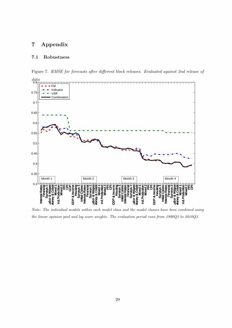
7 Appendix
7.1 Robustness
Figure 7. RMSE for forecasts after different block releases. Evaluated against 2nd release of
data
0.3
0.35
0.4
0.45
0.5
0.55
0.6
0.65
0.7
0.75
0.8
Inte
rest
Rat
es
Fin
anci
al
Sur
veys
2
Labo
r &
Wag
es
Mon
ey &
Cre
dit
Mix
ed 1
In
d.P
rodu
ctio
n M
ixed
2
PP
I C
PI
GD
P
GD
P &
Inco
me
Hou
sing
S
urve
ys 1
In
itial
Cla
ims
Inte
rest
Rat
es
Fin
anci
al
Sur
veys
2
Labo
r &
Wag
es
Mon
ey &
Cre
dit
Mix
ed 1
In
d.P
rodu
ctio
n M
ixed
2
PP
I C
PI
GD
P &
Inco
me
Hou
sing
S
urve
ys 1
In
itial
Cla
ims
Inte
rest
Rat
es
Fin
anci
al
Sur
veys
2
Labo
r &
Wag
es
Mon
ey &
Cre
dit
Mix
ed 1
In
d.P
rodu
ctio
n M
ixed
2
PP
I C
PI
GD
P &
Inco
me
Hou
sing
S
urve
ys 1
In
itial
Cla
ims
Inte
rest
Rat
es
Fin
anci
al
Sur
veys
2
Labo
r &
Wag
es
Mon
ey &
Cre
dit
Mix
ed 1
In
d.P
rodu
ctio
n M
ixed
2
PP
I C
PI
Inte
rest
Rat
es
Fin
anci
al
Sur
veys
2
Labo
r &
Wag
es
Mon
ey &
Cre
dit
Mix
ed 1
In
d.P
rodu
ctio
n M
ixed
2
PP
I C
PI
GD
P
GD
P &
Inco
me
Hou
sing
S
urve
ys 1
In
itial
Cla
ims
Inte
rest
Rat
es
Fin
anci
al
Sur
veys
2
Labo
r &
Wag
es
Mon
ey &
Cre
dit
Mix
ed 1
In
d.P
rodu
ctio
n M
ixed
2
PP
I C
PI
GD
P &
Inco
me
Hou
sing
S
urve
ys 1
In
itial
Cla
ims
Inte
rest
Rat
es
Fin
anci
al
Sur
veys
2
Labo
r &
Wag
es
Mon
ey &
Cre
dit
Mix
ed 1
In
d.P
rodu
ctio
n M
ixed
2
PP
I C
PI
GD
P &
Inco
me
Hou
sing
S
urve
ys 1
In
itial
Cla
ims
Inte
rest
Rat
es
Fin
anci
al
Sur
veys
2
Labo
r &
Wag
es
Mon
ey &
Cre
dit
Mix
ed 1
In
d.P
rodu
ctio
n M
ixed
2
PP
I C
PI
Inte
rest
Rat
es
Fin
anci
al
Sur
veys
2
Labo
r &
Wag
es
Mon
ey &
Cre
dit
Mix
ed 1
In
d.P
rodu
ctio
n M
ixed
2
PP
I C
PI
GD
P
GD
P &
Inco
me
Hou
sing
S
urve
ys 1
In
itial
Cla
ims
Inte
rest
Rat
es
Fin
anci
al
Sur
veys
2
Labo
r &
Wag
es
Mon
ey &
Cre
dit
Mix
ed 1
In
d.P
rodu
ctio
n M
ixed
2
PP
I C
PI
GD
P &
Inco
me
Hou
sing
S
urve
ys 1
In
itial
Cla
ims
Inte
rest
Rat
es
Fin
anci
al
Sur
veys
2
Labo
r &
Wag
es
Mon
ey &
Cre
dit
Mix
ed 1
In
d.P
rodu
ctio
n M
ixed
2
PP
I C
PI
GD
P &
Inco
me
Hou
sing
S
urve
ys 1
In
itial
Cla
ims
Inte
rest
Rat
es
Fin
anci
al
Sur
veys
2
Labo
r &
Wag
es
Mon
ey &
Cre
dit
Mix
ed 1
In
d.P
rodu
ctio
n M
ixed
2
PP
I C
PI
Inte
rest
Rat
es
Fin
anci
al
Sur
veys
2
Labo
r &
Wag
es
Mon
ey &
Cre
dit
Mix
ed 1
In
d.P
rodu
ctio
n M
ixed
2
PP
I C
PI
GD
P
GD
P &
Inco
me
Hou
sing
S
urve
ys 1
In
itial
Cla
ims
Inte
rest
Rat
es
Fin
anci
al
Sur
veys
2
Labo
r &
Wag
es
Mon
ey &
Cre
dit
Mix
ed 1
In
d.P
rodu
ctio
n M
ixed
2
PP
I C
PI
GD
P &
Inco
me
Hou
sing
S
urve
ys 1
In
itial
Cla
ims
Inte
rest
Rat
es
Fin
anci
al
Sur
veys
2
Labo
r &
Wag
es
Mon
ey &
Cre
dit
Mix
ed 1
In
d.P
rodu
ctio
n M
ixed
2
PP
I C
PI
GD
P &
Inco
me
Hou
sing
S
urve
ys 1
In
itial
Cla
ims
Inte
rest
Rat
es
Fin
anci
al
Sur
veys
2
Labo
r &
Wag
es
Mon
ey &
Cre
dit
Mix
ed 1
In
d.P
rodu
ctio
n M
ixed
2
PP
I C
PI
Nowcasting YFN for US. RMSE for model classes and combination adding different blocks of information
FMIndicatorVARCombination
Month 1 Month 2 Month 3 Month 4
Note: The individual models within each model class and the model classes have been combined using
the linear opinion pool and log score weights. The evaluation period runs from 1990Q2 to 2010Q3.
29

Figure 8. Average log scores (inverted) for forecasts after different block releases. Evaluated
against 2nd release of data.
0
0.2
0.4
0.6
0.8
1
1.2
1.4
1.6
Inte
rest
Rat
es
Fin
anci
al
Sur
veys
2
Labo
r &
Wag
es
Mon
ey &
Cre
dit
Mix
ed 1
In
d.P
rodu
ctio
n M
ixed
2
PP
I C
PI
GD
P
GD
P &
Inco
me
Hou
sing
S
urve
ys 1
In
itial
Cla
ims
Inte
rest
Rat
es
Fin
anci
al
Sur
veys
2
Labo
r &
Wag
es
Mon
ey &
Cre
dit
Mix
ed 1
In
d.P
rodu
ctio
n M
ixed
2
PP
I C
PI
GD
P &
Inco
me
Hou
sing
S
urve
ys 1
In
itial
Cla
ims
Inte
rest
Rat
es
Fin
anci
al
Sur
veys
2
Labo
r &
Wag
es
Mon
ey &
Cre
dit
Mix
ed 1
In
d.P
rodu
ctio
n M
ixed
2
PP
I C
PI
GD
P &
Inco
me
Hou
sing
S
urve
ys 1
In
itial
Cla
ims
Inte
rest
Rat
es
Fin
anci
al
Sur
veys
2
Labo
r &
Wag
es
Mon
ey &
Cre
dit
Mix
ed 1
In
d.P
rodu
ctio
n M
ixed
2
PP
I C
PI
Nowcasting GDP for US. Average logarithmic score (inverted) for Combination adding different blocks of information
(a) Combined forecast
0
0.2
0.4
0.6
0.8
1
1.2
1.4
1.6
Inte
rest
Rat
es
Fin
anci
al
Sur
veys
2
Labo
r &
Wag
es
Mon
ey &
Cre
dit
Mix
ed 1
In
d.P
rodu
ctio
n M
ixed
2
PP
I C
PI
GD
P
GD
P &
Inco
me
Hou
sing
S
urve
ys 1
In
itial
Cla
ims
Inte
rest
Rat
es
Fin
anci
al
Sur
veys
2
Labo
r &
Wag
es
Mon
ey &
Cre
dit
Mix
ed 1
In
d.P
rodu
ctio
n M
ixed
2
PP
I C
PI
GD
P &
Inco
me
Hou
sing
S
urve
ys 1
In
itial
Cla
ims
Inte
rest
Rat
es
Fin
anci
al
Sur
veys
2
Labo
r &
Wag
es
Mon
ey &
Cre
dit
Mix
ed 1
In
d.P
rodu
ctio
n M
ixed
2
PP
I C
PI
GD
P &
Inco
me
Hou
sing
S
urve
ys 1
In
itial
Cla
ims
Inte
rest
Rat
es
Fin
anci
al
Sur
veys
2
Labo
r &
Wag
es
Mon
ey &
Cre
dit
Mix
ed 1
In
d.P
rodu
ctio
n M
ixed
2
PP
I C
PI
Nowcasting GDP for US. Average logarithmic score (inverted) for VAR adding different blocks of information
(b) VARs
0
0.2
0.4
0.6
0.8
1
1.2
1.4
1.6
Inte
rest
Rat
es
Fin
anci
al
Sur
veys
2
Labo
r &
Wag
es
Mon
ey &
Cre
dit
Mix
ed 1
In
d.P
rodu
ctio
n M
ixed
2
PP
I C
PI
GD
P
GD
P &
Inco
me
Hou
sing
S
urve
ys 1
In
itial
Cla
ims
Inte
rest
Rat
es
Fin
anci
al
Sur
veys
2
Labo
r &
Wag
es
Mon
ey &
Cre
dit
Mix
ed 1
In
d.P
rodu
ctio
n M
ixed
2
PP
I C
PI
GD
P &
Inco
me
Hou
sing
S
urve
ys 1
In
itial
Cla
ims
Inte
rest
Rat
es
Fin
anci
al
Sur
veys
2
Labo
r &
Wag
es
Mon
ey &
Cre
dit
Mix
ed 1
In
d.P
rodu
ctio
n M
ixed
2
PP
I C
PI
GD
P &
Inco
me
Hou
sing
S
urve
ys 1
In
itial
Cla
ims
Inte
rest
Rat
es
Fin
anci
al
Sur
veys
2
Labo
r &
Wag
es
Mon
ey &
Cre
dit
Mix
ed 1
In
d.P
rodu
ctio
n M
ixed
2
PP
I C
PI
Nowcasting GDP for US. Average logarithmic score (inverted) for FM adding different blocks of information
(c) FM
0
0.2
0.4
0.6
0.8
1
1.2
1.4
1.6
Inte
rest
Rat
es
Fin
anci
al
Sur
veys
2
Labo
r &
Wag
es
Mon
ey &
Cre
dit
Mix
ed 1
In
d.P
rodu
ctio
n M
ixed
2
PP
I C
PI
GD
P
GD
P &
Inco
me
Hou
sing
S
urve
ys 1
In
itial
Cla
ims
Inte
rest
Rat
es
Fin
anci
al
Sur
veys
2
Labo
r &
Wag
es
Mon
ey &
Cre
dit
Mix
ed 1
In
d.P
rodu
ctio
n M
ixed
2
PP
I C
PI
GD
P &
Inco
me
Hou
sing
S
urve
ys 1
In
itial
Cla
ims
Inte
rest
Rat
es
Fin
anci
al
Sur
veys
2
Labo
r &
Wag
es
Mon
ey &
Cre
dit
Mix
ed 1
In
d.P
rodu
ctio
n M
ixed
2
PP
I C
PI
GD
P &
Inco
me
Hou
sing
S
urve
ys 1
In
itial
Cla
ims
Inte
rest
Rat
es
Fin
anci
al
Sur
veys
2
Labo
r &
Wag
es
Mon
ey &
Cre
dit
Mix
ed 1
In
d.P
rodu
ctio
n M
ixed
2
PP
I C
PI
Nowcasting GDP for US. Average logarithmic score (inverted) for Indicator adding different blocks of information
(d) Indicator
Note: The individual models within each model class and the model classes have been combined using
the linear opinion pool and log score weights. The evaluation period runs from 1990Q2 to 2010Q3.
30

Figure 9. Mean square forecasting errors made after different block releases. Evaluated
against 2nd release of data.
0
0.1
0.2
0.3
0.4
0.5
0.6
0.7
0.8
Inte
rest
Rat
es
Fin
anci
al
Sur
veys
2
Labo
r &
Wag
es
Mon
ey &
Cre
dit
Mix
ed 1
In
d.P
rodu
ctio
n M
ixed
2
PP
I C
PI
GD
P
GD
P &
Inco
me
Hou
sing
S
urve
ys 1
In
itial
Cla
ims
Inte
rest
Rat
es
Fin
anci
al
Sur
veys
2
Labo
r &
Wag
es
Mon
ey &
Cre
dit
Mix
ed 1
In
d.P
rodu
ctio
n M
ixed
2
PP
I C
PI
GD
P &
Inco
me
Hou
sing
S
urve
ys 1
In
itial
Cla
ims
Inte
rest
Rat
es
Fin
anci
al
Sur
veys
2
Labo
r &
Wag
es
Mon
ey &
Cre
dit
Mix
ed 1
In
d.P
rodu
ctio
n M
ixed
2
PP
I C
PI
GD
P &
Inco
me
Hou
sing
S
urve
ys 1
In
itial
Cla
ims
Inte
rest
Rat
es
Fin
anci
al
Sur
veys
2
Labo
r &
Wag
es
Mon
ey &
Cre
dit
Mix
ed 1
In
d.P
rodu
ctio
n M
ixed
2
PP
I C
PI
Nowcasting GDP for US. RMSE for Combination adding different blocks of information
(a) Combined forecast
0
0.1
0.2
0.3
0.4
0.5
0.6
0.7
0.8
Inte
rest
Rat
es
Fin
anci
al
Sur
veys
2
Labo
r &
Wag
es
Mon
ey &
Cre
dit
Mix
ed 1
In
d.P
rodu
ctio
n M
ixed
2
PP
I C
PI
GD
P
GD
P &
Inco
me
Hou
sing
S
urve
ys 1
In
itial
Cla
ims
Inte
rest
Rat
es
Fin
anci
al
Sur
veys
2
Labo
r &
Wag
es
Mon
ey &
Cre
dit
Mix
ed 1
In
d.P
rodu
ctio
n M
ixed
2
PP
I C
PI
GD
P &
Inco
me
Hou
sing
S
urve
ys 1
In
itial
Cla
ims
Inte
rest
Rat
es
Fin
anci
al
Sur
veys
2
Labo
r &
Wag
es
Mon
ey &
Cre
dit
Mix
ed 1
In
d.P
rodu
ctio
n M
ixed
2
PP
I C
PI
GD
P &
Inco
me
Hou
sing
S
urve
ys 1
In
itial
Cla
ims
Inte
rest
Rat
es
Fin
anci
al
Sur
veys
2
Labo
r &
Wag
es
Mon
ey &
Cre
dit
Mix
ed 1
In
d.P
rodu
ctio
n M
ixed
2
PP
I C
PI
Nowcasting GDP for US. RMSE for VAR adding different blocks of information
(b) VARs
0
0.1
0.2
0.3
0.4
0.5
0.6
0.7
0.8
Inte
rest
Rat
es
Fin
anci
al
Sur
veys
2
Labo
r &
Wag
es
Mon
ey &
Cre
dit
Mix
ed 1
In
d.P
rodu
ctio
n M
ixed
2
PP
I C
PI
GD
P
GD
P &
Inco
me
Hou
sing
S
urve
ys 1
In
itial
Cla
ims
Inte
rest
Rat
es
Fin
anci
al
Sur
veys
2
Labo
r &
Wag
es
Mon
ey &
Cre
dit
Mix
ed 1
In
d.P
rodu
ctio
n M
ixed
2
PP
I C
PI
GD
P &
Inco
me
Hou
sing
S
urve
ys 1
In
itial
Cla
ims
Inte
rest
Rat
es
Fin
anci
al
Sur
veys
2
Labo
r &
Wag
es
Mon
ey &
Cre
dit
Mix
ed 1
In
d.P
rodu
ctio
n M
ixed
2
PP
I C
PI
GD
P &
Inco
me
Hou
sing
S
urve
ys 1
In
itial
Cla
ims
Inte
rest
Rat
es
Fin
anci
al
Sur
veys
2
Labo
r &
Wag
es
Mon
ey &
Cre
dit
Mix
ed 1
In
d.P
rodu
ctio
n M
ixed
2
PP
I C
PI
Nowcasting GDP for US. RMSE for FM adding different blocks of information
(c) FM
0
0.1
0.2
0.3
0.4
0.5
0.6
0.7
0.8
Inte
rest
Rat
es
Fin
anci
al
Sur
veys
2
Labo
r &
Wag
es
Mon
ey &
Cre
dit
Mix
ed 1
In
d.P
rodu
ctio
n M
ixed
2
PP
I C
PI
GD
P
GD
P &
Inco
me
Hou
sing
S
urve
ys 1
In
itial
Cla
ims
Inte
rest
Rat
es
Fin
anci
al
Sur
veys
2
Labo
r &
Wag
es
Mon
ey &
Cre
dit
Mix
ed 1
In
d.P
rodu
ctio
n M
ixed
2
PP
I C
PI
GD
P &
Inco
me
Hou
sing
S
urve
ys 1
In
itial
Cla
ims
Inte
rest
Rat
es
Fin
anci
al
Sur
veys
2
Labo
r &
Wag
es
Mon
ey &
Cre
dit
Mix
ed 1
In
d.P
rodu
ctio
n M
ixed
2
PP
I C
PI
GD
P &
Inco
me
Hou
sing
S
urve
ys 1
In
itial
Cla
ims
Inte
rest
Rat
es
Fin
anci
al
Sur
veys
2
Labo
r &
Wag
es
Mon
ey &
Cre
dit
Mix
ed 1
In
d.P
rodu
ctio
n M
ixed
2
PP
I C
PI
Nowcasting GDP for US. RMSE for Indicator adding different blocks of information
(d) Indicator
Note: The individual models within each model class and the model classes have been combined using
the linear opinion pool and log score weights. The evaluation period runs from 1990Q2 to 2010Q3.
31

Figure 10. Results when evaluated against 5th release of data.
0.3
0.35
0.4
0.45
0.5
0.55
0.6
0.65
0.7
0.75
0.8
Inte
rest
Rat
es
Fin
anci
al
Sur
veys
2
Labo
r &
Wag
es
Mon
ey &
Cre
dit
Mix
ed 1
In
d.P
rodu
ctio
n M
ixed
2
PP
I C
PI
GD
P
GD
P &
Inco
me
Hou
sing
S
urve
ys 1
In
itial
Cla
ims
Inte
rest
Rat
es
Fin
anci
al
Sur
veys
2
Labo
r &
Wag
es
Mon
ey &
Cre
dit
Mix
ed 1
In
d.P
rodu
ctio
n M
ixed
2
PP
I C
PI
GD
P &
Inco
me
Hou
sing
S
urve
ys 1
In
itial
Cla
ims
Inte
rest
Rat
es
Fin
anci
al
Sur
veys
2
Labo
r &
Wag
es
Mon
ey &
Cre
dit
Mix
ed 1
In
d.P
rodu
ctio
n M
ixed
2
PP
I C
PI
GD
P &
Inco
me
Hou
sing
S
urve
ys 1
In
itial
Cla
ims
Inte
rest
Rat
es
Fin
anci
al
Sur
veys
2
Labo
r &
Wag
es
Mon
ey &
Cre
dit
Mix
ed 1
In
d.P
rodu
ctio
n M
ixed
2
PP
I C
PI
Inte
rest
Rat
es
Fin
anci
al
Sur
veys
2
Labo
r &
Wag
es
Mon
ey &
Cre
dit
Mix
ed 1
In
d.P
rodu
ctio
n M
ixed
2
PP
I C
PI
GD
P
GD
P &
Inco
me
Hou
sing
S
urve
ys 1
In
itial
Cla
ims
Inte
rest
Rat
es
Fin
anci
al
Sur
veys
2
Labo
r &
Wag
es
Mon
ey &
Cre
dit
Mix
ed 1
In
d.P
rodu
ctio
n M
ixed
2
PP
I C
PI
GD
P &
Inco
me
Hou
sing
S
urve
ys 1
In
itial
Cla
ims
Inte
rest
Rat
es
Fin
anci
al
Sur
veys
2
Labo
r &
Wag
es
Mon
ey &
Cre
dit
Mix
ed 1
In
d.P
rodu
ctio
n M
ixed
2
PP
I C
PI
GD
P &
Inco
me
Hou
sing
S
urve
ys 1
In
itial
Cla
ims
Inte
rest
Rat
es
Fin
anci
al
Sur
veys
2
Labo
r &
Wag
es
Mon
ey &
Cre
dit
Mix
ed 1
In
d.P
rodu
ctio
n M
ixed
2
PP
I C
PI
Inte
rest
Rat
es
Fin
anci
al
Sur
veys
2
Labo
r &
Wag
es
Mon
ey &
Cre
dit
Mix
ed 1
In
d.P
rodu
ctio
n M
ixed
2
PP
I C
PI
GD
P
GD
P &
Inco
me
Hou
sing
S
urve
ys 1
In
itial
Cla
ims
Inte
rest
Rat
es
Fin
anci
al
Sur
veys
2
Labo
r &
Wag
es
Mon
ey &
Cre
dit
Mix
ed 1
In
d.P
rodu
ctio
n M
ixed
2
PP
I C
PI
GD
P &
Inco
me
Hou
sing
S
urve
ys 1
In
itial
Cla
ims
Inte
rest
Rat
es
Fin
anci
al
Sur
veys
2
Labo
r &
Wag
es
Mon
ey &
Cre
dit
Mix
ed 1
In
d.P
rodu
ctio
n M
ixed
2
PP
I C
PI
GD
P &
Inco
me
Hou
sing
S
urve
ys 1
In
itial
Cla
ims
Inte
rest
Rat
es
Fin
anci
al
Sur
veys
2
Labo
r &
Wag
es
Mon
ey &
Cre
dit
Mix
ed 1
In
d.P
rodu
ctio
n M
ixed
2
PP
I C
PI
Inte
rest
Rat
es
Fin
anci
al
Sur
veys
2
Labo
r &
Wag
es
Mon
ey &
Cre
dit
Mix
ed 1
In
d.P
rodu
ctio
n M
ixed
2
PP
I C
PI
GD
P
GD
P &
Inco
me
Hou
sing
S
urve
ys 1
In
itial
Cla
ims
Inte
rest
Rat
es
Fin
anci
al
Sur
veys
2
Labo
r &
Wag
es
Mon
ey &
Cre
dit
Mix
ed 1
In
d.P
rodu
ctio
n M
ixed
2
PP
I C
PI
GD
P &
Inco
me
Hou
sing
S
urve
ys 1
In
itial
Cla
ims
Inte
rest
Rat
es
Fin
anci
al
Sur
veys
2
Labo
r &
Wag
es
Mon
ey &
Cre
dit
Mix
ed 1
In
d.P
rodu
ctio
n M
ixed
2
PP
I C
PI
GD
P &
Inco
me
Hou
sing
S
urve
ys 1
In
itial
Cla
ims
Inte
rest
Rat
es
Fin
anci
al
Sur
veys
2
Labo
r &
Wag
es
Mon
ey &
Cre
dit
Mix
ed 1
In
d.P
rodu
ctio
n M
ixed
2
PP
I C
PI
Nowcasting YFN for US. RMSE for model classes and combination adding different blocks of information
FMIndicatorVARCombination
Month 1 Month 2 Month 3 Month 4
(a) RMSE
−1.3
−1.2
−1.1
−1
−0.9
−0.8
−0.7
−0.6
−0.5
−0.4
Inte
rest
Rat
es
Fin
anci
al
Sur
veys
2
Labo
r &
Wag
es
Mon
ey &
Cre
dit
Mix
ed 1
In
d.P
rodu
ctio
n M
ixed
2
PP
I C
PI
GD
P
GD
P &
Inco
me
Hou
sing
S
urve
ys 1
In
itial
Cla
ims
Inte
rest
Rat
es
Fin
anci
al
Sur
veys
2
Labo
r &
Wag
es
Mon
ey &
Cre
dit
Mix
ed 1
In
d.P
rodu
ctio
n M
ixed
2
PP
I C
PI
GD
P &
Inco
me
Hou
sing
S
urve
ys 1
In
itial
Cla
ims
Inte
rest
Rat
es
Fin
anci
al
Sur
veys
2
Labo
r &
Wag
es
Mon
ey &
Cre
dit
Mix
ed 1
In
d.P
rodu
ctio
n M
ixed
2
PP
I C
PI
GD
P &
Inco
me
Hou
sing
S
urve
ys 1
In
itial
Cla
ims
Inte
rest
Rat
es
Fin
anci
al
Sur
veys
2
Labo
r &
Wag
es
Mon
ey &
Cre
dit
Mix
ed 1
In
d.P
rodu
ctio
n M
ixed
2
PP
I C
PI
Inte
rest
Rat
es
Fin
anci
al
Sur
veys
2
Labo
r &
Wag
es
Mon
ey &
Cre
dit
Mix
ed 1
In
d.P
rodu
ctio
n M
ixed
2
PP
I C
PI
GD
P
GD
P &
Inco
me
Hou
sing
S
urve
ys 1
In
itial
Cla
ims
Inte
rest
Rat
es
Fin
anci
al
Sur
veys
2
Labo
r &
Wag
es
Mon
ey &
Cre
dit
Mix
ed 1
In
d.P
rodu
ctio
n M
ixed
2
PP
I C
PI
GD
P &
Inco
me
Hou
sing
S
urve
ys 1
In
itial
Cla
ims
Inte
rest
Rat
es
Fin
anci
al
Sur
veys
2
Labo
r &
Wag
es
Mon
ey &
Cre
dit
Mix
ed 1
In
d.P
rodu
ctio
n M
ixed
2
PP
I C
PI
GD
P &
Inco
me
Hou
sing
S
urve
ys 1
In
itial
Cla
ims
Inte
rest
Rat
es
Fin
anci
al
Sur
veys
2
Labo
r &
Wag
es
Mon
ey &
Cre
dit
Mix
ed 1
In
d.P
rodu
ctio
n M
ixed
2
PP
I C
PI
Inte
rest
Rat
es
Fin
anci
al
Sur
veys
2
Labo
r &
Wag
es
Mon
ey &
Cre
dit
Mix
ed 1
In
d.P
rodu
ctio
n M
ixed
2
PP
I C
PI
GD
P
GD
P &
Inco
me
Hou
sing
S
urve
ys 1
In
itial
Cla
ims
Inte
rest
Rat
es
Fin
anci
al
Sur
veys
2
Labo
r &
Wag
es
Mon
ey &
Cre
dit
Mix
ed 1
In
d.P
rodu
ctio
n M
ixed
2
PP
I C
PI
GD
P &
Inco
me
Hou
sing
S
urve
ys 1
In
itial
Cla
ims
Inte
rest
Rat
es
Fin
anci
al
Sur
veys
2
Labo
r &
Wag
es
Mon
ey &
Cre
dit
Mix
ed 1
In
d.P
rodu
ctio
n M
ixed
2
PP
I C
PI
GD
P &
Inco
me
Hou
sing
S
urve
ys 1
In
itial
Cla
ims
Inte
rest
Rat
es
Fin
anci
al
Sur
veys
2
Labo
r &
Wag
es
Mon
ey &
Cre
dit
Mix
ed 1
In
d.P
rodu
ctio
n M
ixed
2
PP
I C
PI
Inte
rest
Rat
es
Fin
anci
al
Sur
veys
2
Labo
r &
Wag
es
Mon
ey &
Cre
dit
Mix
ed 1
In
d.P
rodu
ctio
n M
ixed
2
PP
I C
PI
GD
P
GD
P &
Inco
me
Hou
sing
S
urve
ys 1
In
itial
Cla
ims
Inte
rest
Rat
es
Fin
anci
al
Sur
veys
2
Labo
r &
Wag
es
Mon
ey &
Cre
dit
Mix
ed 1
In
d.P
rodu
ctio
n M
ixed
2
PP
I C
PI
GD
P &
Inco
me
Hou
sing
S
urve
ys 1
In
itial
Cla
ims
Inte
rest
Rat
es
Fin
anci
al
Sur
veys
2
Labo
r &
Wag
es
Mon
ey &
Cre
dit
Mix
ed 1
In
d.P
rodu
ctio
n M
ixed
2
PP
I C
PI
GD
P &
Inco
me
Hou
sing
S
urve
ys 1
In
itial
Cla
ims
Inte
rest
Rat
es
Fin
anci
al
Sur
veys
2
Labo
r &
Wag
es
Mon
ey &
Cre
dit
Mix
ed 1
In
d.P
rodu
ctio
n M
ixed
2
PP
I C
PI
Nowcasting YFN for US. Average logaritmic score for model classes and combination adding different blocks of information
FMIndicatorVARCombination
Month 1 Month 2 Month 3 Month 4
(b) Average log score
0
0.1
0.2
0.3
0.4
0.5
0.6
0.7
0.8
0.9
1
Inte
rest
Rat
es
Fin
anci
al
Sur
veys
2
Labo
r &
Wag
es
Mon
ey &
Cre
dit
Mix
ed 1
In
d.P
rodu
ctio
n M
ixed
2
PP
I C
PI
GD
P
GD
P &
Inco
me
Hou
sing
S
urve
ys 1
In
itial
Cla
ims
Inte
rest
Rat
es
Fin
anci
al
Sur
veys
2
Labo
r &
Wag
es
Mon
ey &
Cre
dit
Mix
ed 1
In
d.P
rodu
ctio
n M
ixed
2
PP
I C
PI
GD
P &
Inco
me
Hou
sing
S
urve
ys 1
In
itial
Cla
ims
Inte
rest
Rat
es
Fin
anci
al
Sur
veys
2
Labo
r &
Wag
es
Mon
ey &
Cre
dit
Mix
ed 1
In
d.P
rodu
ctio
n M
ixed
2
PP
I C
PI
GD
P &
Inco
me
Hou
sing
S
urve
ys 1
In
itial
Cla
ims
Inte
rest
Rat
es
Fin
anci
al
Sur
veys
2
Labo
r &
Wag
es
Mon
ey &
Cre
dit
Mix
ed 1
In
d.P
rodu
ctio
n M
ixed
2
PP
I C
PI
Inte
rest
Rat
es
Fin
anci
al
Sur
veys
2
Labo
r &
Wag
es
Mon
ey &
Cre
dit
Mix
ed 1
In
d.P
rodu
ctio
n M
ixed
2
PP
I C
PI
GD
P
GD
P &
Inco
me
Hou
sing
S
urve
ys 1
In
itial
Cla
ims
Inte
rest
Rat
es
Fin
anci
al
Sur
veys
2
Labo
r &
Wag
es
Mon
ey &
Cre
dit
Mix
ed 1
In
d.P
rodu
ctio
n M
ixed
2
PP
I C
PI
GD
P &
Inco
me
Hou
sing
S
urve
ys 1
In
itial
Cla
ims
Inte
rest
Rat
es
Fin
anci
al
Sur
veys
2
Labo
r &
Wag
es
Mon
ey &
Cre
dit
Mix
ed 1
In
d.P
rodu
ctio
n M
ixed
2
PP
I C
PI
GD
P &
Inco
me
Hou
sing
S
urve
ys 1
In
itial
Cla
ims
Inte
rest
Rat
es
Fin
anci
al
Sur
veys
2
Labo
r &
Wag
es
Mon
ey &
Cre
dit
Mix
ed 1
In
d.P
rodu
ctio
n M
ixed
2
PP
I C
PI
Inte
rest
Rat
es
Fin
anci
al
Sur
veys
2
Labo
r &
Wag
es
Mon
ey &
Cre
dit
Mix
ed 1
In
d.P
rodu
ctio
n M
ixed
2
PP
I C
PI
GD
P
GD
P &
Inco
me
Hou
sing
S
urve
ys 1
In
itial
Cla
ims
Inte
rest
Rat
es
Fin
anci
al
Sur
veys
2
Labo
r &
Wag
es
Mon
ey &
Cre
dit
Mix
ed 1
In
d.P
rodu
ctio
n M
ixed
2
PP
I C
PI
GD
P &
Inco
me
Hou
sing
S
urve
ys 1
In
itial
Cla
ims
Inte
rest
Rat
es
Fin
anci
al
Sur
veys
2
Labo
r &
Wag
es
Mon
ey &
Cre
dit
Mix
ed 1
In
d.P
rodu
ctio
n M
ixed
2
PP
I C
PI
GD
P &
Inco
me
Hou
sing
S
urve
ys 1
In
itial
Cla
ims
Inte
rest
Rat
es
Fin
anci
al
Sur
veys
2
Labo
r &
Wag
es
Mon
ey &
Cre
dit
Mix
ed 1
In
d.P
rodu
ctio
n M
ixed
2
PP
I C
PI
Nowcasting YFN for US. Weights for model classes in combination when adding different blocks of information
FMIndicatorVAR
(c) Weights
0 0.1 0.2 0.3 0.4 0.5 0.6 0.7 0.8 0.9 10
2
4
6
8
10
12
14
16
18
20PITs
Probability integral transforms
Fre
quen
cy (
# of
obs
erva
tions
)
m0 m1 m2 m3 m4
(d) Pits
Note: The individual models within each model class and the model classes have been combined using
the linear opinion pool and log score weights. The evaluation period runs from 1990Q2 to 2010Q3.
32
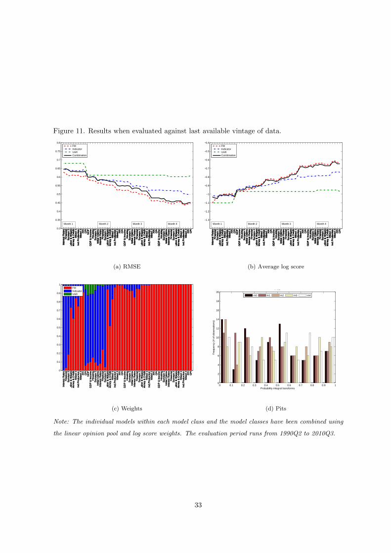
Figure 11. Results when evaluated against last available vintage of data.
0.3
0.35
0.4
0.45
0.5
0.55
0.6
0.65
0.7
0.75
0.8
Inte
rest
Rat
es
Fin
anci
al
Sur
veys
2
Labo
r &
Wag
es
Mon
ey &
Cre
dit
Mix
ed 1
In
d.P
rodu
ctio
n M
ixed
2
PP
I C
PI
GD
P
GD
P &
Inco
me
Hou
sing
S
urve
ys 1
In
itial
Cla
ims
Inte
rest
Rat
es
Fin
anci
al
Sur
veys
2
Labo
r &
Wag
es
Mon
ey &
Cre
dit
Mix
ed 1
In
d.P
rodu
ctio
n M
ixed
2
PP
I C
PI
GD
P &
Inco
me
Hou
sing
S
urve
ys 1
In
itial
Cla
ims
Inte
rest
Rat
es
Fin
anci
al
Sur
veys
2
Labo
r &
Wag
es
Mon
ey &
Cre
dit
Mix
ed 1
In
d.P
rodu
ctio
n M
ixed
2
PP
I C
PI
GD
P &
Inco
me
Hou
sing
S
urve
ys 1
In
itial
Cla
ims
Inte
rest
Rat
es
Fin
anci
al
Sur
veys
2
Labo
r &
Wag
es
Mon
ey &
Cre
dit
Mix
ed 1
In
d.P
rodu
ctio
n M
ixed
2
PP
I C
PI
Inte
rest
Rat
es
Fin
anci
al
Sur
veys
2
Labo
r &
Wag
es
Mon
ey &
Cre
dit
Mix
ed 1
In
d.P
rodu
ctio
n M
ixed
2
PP
I C
PI
GD
P
GD
P &
Inco
me
Hou
sing
S
urve
ys 1
In
itial
Cla
ims
Inte
rest
Rat
es
Fin
anci
al
Sur
veys
2
Labo
r &
Wag
es
Mon
ey &
Cre
dit
Mix
ed 1
In
d.P
rodu
ctio
n M
ixed
2
PP
I C
PI
GD
P &
Inco
me
Hou
sing
S
urve
ys 1
In
itial
Cla
ims
Inte
rest
Rat
es
Fin
anci
al
Sur
veys
2
Labo
r &
Wag
es
Mon
ey &
Cre
dit
Mix
ed 1
In
d.P
rodu
ctio
n M
ixed
2
PP
I C
PI
GD
P &
Inco
me
Hou
sing
S
urve
ys 1
In
itial
Cla
ims
Inte
rest
Rat
es
Fin
anci
al
Sur
veys
2
Labo
r &
Wag
es
Mon
ey &
Cre
dit
Mix
ed 1
In
d.P
rodu
ctio
n M
ixed
2
PP
I C
PI
Inte
rest
Rat
es
Fin
anci
al
Sur
veys
2
Labo
r &
Wag
es
Mon
ey &
Cre
dit
Mix
ed 1
In
d.P
rodu
ctio
n M
ixed
2
PP
I C
PI
GD
P
GD
P &
Inco
me
Hou
sing
S
urve
ys 1
In
itial
Cla
ims
Inte
rest
Rat
es
Fin
anci
al
Sur
veys
2
Labo
r &
Wag
es
Mon
ey &
Cre
dit
Mix
ed 1
In
d.P
rodu
ctio
n M
ixed
2
PP
I C
PI
GD
P &
Inco
me
Hou
sing
S
urve
ys 1
In
itial
Cla
ims
Inte
rest
Rat
es
Fin
anci
al
Sur
veys
2
Labo
r &
Wag
es
Mon
ey &
Cre
dit
Mix
ed 1
In
d.P
rodu
ctio
n M
ixed
2
PP
I C
PI
GD
P &
Inco
me
Hou
sing
S
urve
ys 1
In
itial
Cla
ims
Inte
rest
Rat
es
Fin
anci
al
Sur
veys
2
Labo
r &
Wag
es
Mon
ey &
Cre
dit
Mix
ed 1
In
d.P
rodu
ctio
n M
ixed
2
PP
I C
PI
Inte
rest
Rat
es
Fin
anci
al
Sur
veys
2
Labo
r &
Wag
es
Mon
ey &
Cre
dit
Mix
ed 1
In
d.P
rodu
ctio
n M
ixed
2
PP
I C
PI
GD
P
GD
P &
Inco
me
Hou
sing
S
urve
ys 1
In
itial
Cla
ims
Inte
rest
Rat
es
Fin
anci
al
Sur
veys
2
Labo
r &
Wag
es
Mon
ey &
Cre
dit
Mix
ed 1
In
d.P
rodu
ctio
n M
ixed
2
PP
I C
PI
GD
P &
Inco
me
Hou
sing
S
urve
ys 1
In
itial
Cla
ims
Inte
rest
Rat
es
Fin
anci
al
Sur
veys
2
Labo
r &
Wag
es
Mon
ey &
Cre
dit
Mix
ed 1
In
d.P
rodu
ctio
n M
ixed
2
PP
I C
PI
GD
P &
Inco
me
Hou
sing
S
urve
ys 1
In
itial
Cla
ims
Inte
rest
Rat
es
Fin
anci
al
Sur
veys
2
Labo
r &
Wag
es
Mon
ey &
Cre
dit
Mix
ed 1
In
d.P
rodu
ctio
n M
ixed
2
PP
I C
PI
Nowcasting YFN for US. RMSE for model classes and combination adding different blocks of information
FMIndicatorVARCombination
Month 1 Month 2 Month 3 Month 4
(a) RMSE
−1.3
−1.2
−1.1
−1
−0.9
−0.8
−0.7
−0.6
−0.5
−0.4
Inte
rest
Rat
es
Fin
anci
al
Sur
veys
2
Labo
r &
Wag
es
Mon
ey &
Cre
dit
Mix
ed 1
In
d.P
rodu
ctio
n M
ixed
2
PP
I C
PI
GD
P
GD
P &
Inco
me
Hou
sing
S
urve
ys 1
In
itial
Cla
ims
Inte
rest
Rat
es
Fin
anci
al
Sur
veys
2
Labo
r &
Wag
es
Mon
ey &
Cre
dit
Mix
ed 1
In
d.P
rodu
ctio
n M
ixed
2
PP
I C
PI
GD
P &
Inco
me
Hou
sing
S
urve
ys 1
In
itial
Cla
ims
Inte
rest
Rat
es
Fin
anci
al
Sur
veys
2
Labo
r &
Wag
es
Mon
ey &
Cre
dit
Mix
ed 1
In
d.P
rodu
ctio
n M
ixed
2
PP
I C
PI
GD
P &
Inco
me
Hou
sing
S
urve
ys 1
In
itial
Cla
ims
Inte
rest
Rat
es
Fin
anci
al
Sur
veys
2
Labo
r &
Wag
es
Mon
ey &
Cre
dit
Mix
ed 1
In
d.P
rodu
ctio
n M
ixed
2
PP
I C
PI
Inte
rest
Rat
es
Fin
anci
al
Sur
veys
2
Labo
r &
Wag
es
Mon
ey &
Cre
dit
Mix
ed 1
In
d.P
rodu
ctio
n M
ixed
2
PP
I C
PI
GD
P
GD
P &
Inco
me
Hou
sing
S
urve
ys 1
In
itial
Cla
ims
Inte
rest
Rat
es
Fin
anci
al
Sur
veys
2
Labo
r &
Wag
es
Mon
ey &
Cre
dit
Mix
ed 1
In
d.P
rodu
ctio
n M
ixed
2
PP
I C
PI
GD
P &
Inco
me
Hou
sing
S
urve
ys 1
In
itial
Cla
ims
Inte
rest
Rat
es
Fin
anci
al
Sur
veys
2
Labo
r &
Wag
es
Mon
ey &
Cre
dit
Mix
ed 1
In
d.P
rodu
ctio
n M
ixed
2
PP
I C
PI
GD
P &
Inco
me
Hou
sing
S
urve
ys 1
In
itial
Cla
ims
Inte
rest
Rat
es
Fin
anci
al
Sur
veys
2
Labo
r &
Wag
es
Mon
ey &
Cre
dit
Mix
ed 1
In
d.P
rodu
ctio
n M
ixed
2
PP
I C
PI
Inte
rest
Rat
es
Fin
anci
al
Sur
veys
2
Labo
r &
Wag
es
Mon
ey &
Cre
dit
Mix
ed 1
In
d.P
rodu
ctio
n M
ixed
2
PP
I C
PI
GD
P
GD
P &
Inco
me
Hou
sing
S
urve
ys 1
In
itial
Cla
ims
Inte
rest
Rat
es
Fin
anci
al
Sur
veys
2
Labo
r &
Wag
es
Mon
ey &
Cre
dit
Mix
ed 1
In
d.P
rodu
ctio
n M
ixed
2
PP
I C
PI
GD
P &
Inco
me
Hou
sing
S
urve
ys 1
In
itial
Cla
ims
Inte
rest
Rat
es
Fin
anci
al
Sur
veys
2
Labo
r &
Wag
es
Mon
ey &
Cre
dit
Mix
ed 1
In
d.P
rodu
ctio
n M
ixed
2
PP
I C
PI
GD
P &
Inco
me
Hou
sing
S
urve
ys 1
In
itial
Cla
ims
Inte
rest
Rat
es
Fin
anci
al
Sur
veys
2
Labo
r &
Wag
es
Mon
ey &
Cre
dit
Mix
ed 1
In
d.P
rodu
ctio
n M
ixed
2
PP
I C
PI
Inte
rest
Rat
es
Fin
anci
al
Sur
veys
2
Labo
r &
Wag
es
Mon
ey &
Cre
dit
Mix
ed 1
In
d.P
rodu
ctio
n M
ixed
2
PP
I C
PI
GD
P
GD
P &
Inco
me
Hou
sing
S
urve
ys 1
In
itial
Cla
ims
Inte
rest
Rat
es
Fin
anci
al
Sur
veys
2
Labo
r &
Wag
es
Mon
ey &
Cre
dit
Mix
ed 1
In
d.P
rodu
ctio
n M
ixed
2
PP
I C
PI
GD
P &
Inco
me
Hou
sing
S
urve
ys 1
In
itial
Cla
ims
Inte
rest
Rat
es
Fin
anci
al
Sur
veys
2
Labo
r &
Wag
es
Mon
ey &
Cre
dit
Mix
ed 1
In
d.P
rodu
ctio
n M
ixed
2
PP
I C
PI
GD
P &
Inco
me
Hou
sing
S
urve
ys 1
In
itial
Cla
ims
Inte
rest
Rat
es
Fin
anci
al
Sur
veys
2
Labo
r &
Wag
es
Mon
ey &
Cre
dit
Mix
ed 1
In
d.P
rodu
ctio
n M
ixed
2
PP
I C
PI
Nowcasting YFN for US. Average logaritmic score for model classes and combination adding different blocks of information
FMIndicatorVARCombination
Month 1 Month 2 Month 3 Month 4
(b) Average log score
0
0.1
0.2
0.3
0.4
0.5
0.6
0.7
0.8
0.9
1
Inte
rest
Rat
es
Fin
anci
al
Sur
veys
2
Labo
r &
Wag
es
Mon
ey &
Cre
dit
Mix
ed 1
In
d.P
rodu
ctio
n M
ixed
2
PP
I C
PI
GD
P
GD
P &
Inco
me
Hou
sing
S
urve
ys 1
In
itial
Cla
ims
Inte
rest
Rat
es
Fin
anci
al
Sur
veys
2
Labo
r &
Wag
es
Mon
ey &
Cre
dit
Mix
ed 1
In
d.P
rodu
ctio
n M
ixed
2
PP
I C
PI
GD
P &
Inco
me
Hou
sing
S
urve
ys 1
In
itial
Cla
ims
Inte
rest
Rat
es
Fin
anci
al
Sur
veys
2
Labo
r &
Wag
es
Mon
ey &
Cre
dit
Mix
ed 1
In
d.P
rodu
ctio
n M
ixed
2
PP
I C
PI
GD
P &
Inco
me
Hou
sing
S
urve
ys 1
In
itial
Cla
ims
Inte
rest
Rat
es
Fin
anci
al
Sur
veys
2
Labo
r &
Wag
es
Mon
ey &
Cre
dit
Mix
ed 1
In
d.P
rodu
ctio
n M
ixed
2
PP
I C
PI
Inte
rest
Rat
es
Fin
anci
al
Sur
veys
2
Labo
r &
Wag
es
Mon
ey &
Cre
dit
Mix
ed 1
In
d.P
rodu
ctio
n M
ixed
2
PP
I C
PI
GD
P
GD
P &
Inco
me
Hou
sing
S
urve
ys 1
In
itial
Cla
ims
Inte
rest
Rat
es
Fin
anci
al
Sur
veys
2
Labo
r &
Wag
es
Mon
ey &
Cre
dit
Mix
ed 1
In
d.P
rodu
ctio
n M
ixed
2
PP
I C
PI
GD
P &
Inco
me
Hou
sing
S
urve
ys 1
In
itial
Cla
ims
Inte
rest
Rat
es
Fin
anci
al
Sur
veys
2
Labo
r &
Wag
es
Mon
ey &
Cre
dit
Mix
ed 1
In
d.P
rodu
ctio
n M
ixed
2
PP
I C
PI
GD
P &
Inco
me
Hou
sing
S
urve
ys 1
In
itial
Cla
ims
Inte
rest
Rat
es
Fin
anci
al
Sur
veys
2
Labo
r &
Wag
es
Mon
ey &
Cre
dit
Mix
ed 1
In
d.P
rodu
ctio
n M
ixed
2
PP
I C
PI
Inte
rest
Rat
es
Fin
anci
al
Sur
veys
2
Labo
r &
Wag
es
Mon
ey &
Cre
dit
Mix
ed 1
In
d.P
rodu
ctio
n M
ixed
2
PP
I C
PI
GD
P
GD
P &
Inco
me
Hou
sing
S
urve
ys 1
In
itial
Cla
ims
Inte
rest
Rat
es
Fin
anci
al
Sur
veys
2
Labo
r &
Wag
es
Mon
ey &
Cre
dit
Mix
ed 1
In
d.P
rodu
ctio
n M
ixed
2
PP
I C
PI
GD
P &
Inco
me
Hou
sing
S
urve
ys 1
In
itial
Cla
ims
Inte
rest
Rat
es
Fin
anci
al
Sur
veys
2
Labo
r &
Wag
es
Mon
ey &
Cre
dit
Mix
ed 1
In
d.P
rodu
ctio
n M
ixed
2
PP
I C
PI
GD
P &
Inco
me
Hou
sing
S
urve
ys 1
In
itial
Cla
ims
Inte
rest
Rat
es
Fin
anci
al
Sur
veys
2
Labo
r &
Wag
es
Mon
ey &
Cre
dit
Mix
ed 1
In
d.P
rodu
ctio
n M
ixed
2
PP
I C
PI
Nowcasting YFN for US. Weights for model classes in combination when adding different blocks of information
FMIndicatorVAR
(c) Weights
0 0.1 0.2 0.3 0.4 0.5 0.6 0.7 0.8 0.9 10
2
4
6
8
10
12
14
16
18
20PITs
Probability integral transforms
Fre
quen
cy (
# of
obs
erva
tions
)
m0 m1 m2 m3 m4
(d) Pits
Note: The individual models within each model class and the model classes have been combined using
the linear opinion pool and log score weights. The evaluation period runs from 1990Q2 to 2010Q3.
33

7.2 Models and model classes
Table 1 in the main text gives a brief description of the three model classes and individual
models within each class that are included in this analysis. A more thorough description of
each model class and the different specifications is given below.
7.2.1 Vector Autoregressive models (VAR)
VAR models, first introduced by Sims (1980), are arguably the most commonly used model
class for economic analysis and forecasting by policymakers. Assume we have the following
general model
Yt = α+
p∑i=1
βiYt−i + εt, εt ∼ N(0,Σε), (8)
where Yt = (y1,t, y2,t). We include four different quarterly VAR models, where y1,t always
denotes GDP, while y2,t is either empty (AR model) or contains CPI inflation and/or the
Federal funds rate. For each of the four models we consider three different transformations of
the data; first differences, double differences and detrended (using an exponential smoother).
As VARs may be prone to instabilities, both full-sample and two different rolling-sample
VARs are estimated. The two rolling-samples are set to 20 and 30 quarters. Finally, we let
the lag length p vary from 1 to 4. In total, we consider 36 AR models, 72 bivariate VARs and
36 trivariate VARs. We refer to these models as the VARs.
Several papers such as, Evans (2005), Giannone et al. (2008) and Aruoba et al. (2009),
show that accounting for the timeliness of data is crucial for nowcasting. That is, the ex-
ploitation of timely information leads to improvement in the nowcast accuracy. Taking into
account the flow of data releases is therefore essential to our analysis. In the case of the VARs,
both quarterly CPI inflation and quarterly averages of the Federal funds rate are available
prior to the GDP release. The models are put into a state space form and hence Kalman
filter techniques can easily be applied to deal with missing data, i.e. the unbalanced data
problem. This is also a key aspect when constructing the predictive densities from the dif-
ferent models. The forecast uncertainties are obtained through simulations, where the final
densities are derived using kernel smoothing techniques. By applying the Kalman filter we
can obtain conditional forecasts when the data set is unbalanced. More precisely, we use the
smoothed covariance matrix of the predictors, which will resemble the mean squared error
34
(MSE) matrix of the system, and draw from the normal distribution to obtain simulated
forecasts for each horizon.22 This is explained in more detail in appendix section 7.3.
7.2.2 Leading indicator models (LIM)
There is a large amount of studies showing that leading indicators are useful for economic
forecasting, see among others Banerjee et al. (2005), Banerjee and Marcellino (2006) and
Marcellino (2006) for a survey on the use of leading indicators in macroeconomics.
We include in total 120 leading indicators for U.S. GDP. For each leading indicator we
construct a bivariate VAR as described in equation 8, where y2,t now will denote the leading
indicator. As with the VARs, both full-sample and two different rolling-sample models are
estimated. The rolling-samples are set to 20 and 30 quarters. All the leading indicators
included here are of monthly frequency. Hence, we need to bridge the monthly indicators
with quarterly GDP. This is done by constructing quarterly averages of the monthly series.
If a monthly series only contains one or two months of a quarter, we simply construct the
average of the one or two observations from the quarter of interest.23 The unbalanced data
set problem and the construction of the predictive densities are then handled in the same way
as described for the VARs above.
7.2.3 Factor Models (FM)
Factor models have become increasingly popular at central banks as they tend to have good
forecasting properties, benefitting from exploiting information from large datasets. See among
others Stock and Watson (2002) and Giannone et al. (2008).
The objective of factor models is to summarize the information contained in large datasets,
while at the same time reducing their dimension. In other words; to reduce the parameter
space. The model that we consider is an approximate dynamic factor model similar to Gian-
none et al. (2008). This is a model that accounts for the unbalanced data set problem. Assume
we have a vector of n stationary monthly variables Xt =(x1t, . . . , xnt
)′, t = 1, ..., T ,
which have been standardized to have mean equal to zero and variance equal to one. The
22See for example Lutkepohl (2005).23See Baffigi et al. (2004) and Angelini et al. (2011) for a more detailed discussion of alternative bridge
equations.
35

model is given by the following two equations.
Xt = χt + ξt = ΛFt + ξt, ξt ∼ N(0,Σξ) (9)
Ft =
p∑i=1
AiFt−i +But, ut ∼ N(0, Iu) (10)
Equation 9 relates the monthly time series Xt to a common component χt plus an idiosyncratic
component ξt = (ξ1,t, . . . , ξn,t)′. The former is given by an r × 1 vector of latent factors
Ft = (f1,t, . . . , fr,t)′ times an n× r matrix of factor loadings Λ, while the latter is assumed to
be multivariate white noise. Equation 10 describes the law of motion for the latent factors.
The factors are driven by q-dimensional standardized white noise ut, where B is an r × q
matrix, where q ≤ r. Finally, A1, . . . , Ap are r × r matrices of parameters.
Our task is to nowcast quarterly GDP growth (yQt ). We therefore need to build a bridge
between the monthly variables and the quarterly GDP. All monthly variables are transformed
to ensure that the corresponding quarterly quantities are given by xQi,t ∼ (xi,t+xi,t−1 +xi,t−2)
measured at the last month of each quarter, i.e. t = 3k and k = 1, . . . , T/3. This implies
that series in differences enter the factor model in terms of three-month changes. Defining
the quarterly factors as FQt = (Ft + Ft−1 + Ft−2), the factors-based bridge equation follows:
yQt = α+ β′FQt + et, et ∼ N(0,Σe) (11)
where β is an r × 1 vector of parameters.
The model is estimated in a two-step procedure using principal components and the
Kalman filter. The unbalanced part of the data set can be incorporated through the use
of the Kalman filter, where missing observations are interpreted to have an infinitely large
noise to signal ratio. For more details about this, see Giannone et al. (2008).
The simulated forecasts from the dynamic factor model are derived using a small modifi-
cation of the technique described for the VARs above. The factors are derived and forecasted
using the Kalman filter, while the forecasting equation itself is direct, and conditional on the
factors. Uncertainty in the factor forecasts are taken into account in the forecasting equation.
The factor uncertainty is drawn from the normal distribution, using the smoothed covariance
matrix from the Kalman Filter in the same manner as described above. The uncertainty in the
forecasting equation is derived through drawing a random shock from the normal distribution
of past residuals.
36

7.3 The Kalman Filter: An example with a bivariate VAR
Assume we have the following bivariate VAR:
y1,t
y2,t
=
c1
c2
+
β11 β12
β21 β22
y1,t−1
y2,t−1
+
u1,t
u2,t
(12)
which can be written as:
Yt = C + βYt−1 + Ut (13)
If we put our VAR into a State Space form we will get the following equations:
State equation
αt = βαt−1 + C + Ut (14)
Observation equation
Yt = αt (15)
In our application we have two different cases; a balanced VAR and an unbalanced VAR.
Balanced VAR
In the case with a balanced data set, we will have the following prediction equations
αt|t−1 = βαt−1|t−1 + C (16)
Pt|t−1 = βPt−1|t−1β′ +Q (17)
vt|t−1 = Yt − Yt|t−1 = Yt − αt|t−1 (18)
Ft|t−1 = Pt−1|t−1 (19)
37

and the following updating equations
αt|t = αt|t−1 +Ktvt|t−1 (20)
Pt|t = Pt|t−1 −KtZtPt|t−1 (21)
In the case where we perfectly observe the state K = 1, while in the case where we are
forecasting, K = 0. Note that the the variance of the prediction error increases when the
forecasting horizon increases.
Unbalanced VAR
Assume that we now observe y2,t, but not y1,t. In this case we have an unbalanced VAR.
In this case the prediction equations 16 and 17 still holds, while equation 18 and 19 changes
to
vt|t−1 = Yt − Yt|t−1 = WtYt − Ztαt|t−1 (22)
with Wt =
0
1
′, since Y1,t is now not observed.
Ft|t−1 = WtPt−1|t−1W′t = V ar(u2) (23)
and the following updating equations
αt|t = αt|t−1 +Ktvt|t−1 = αt|t−1 + Pt|t−1Z′tW′tFt|t−1vt|t−1 (24)
Pt|t = Pt|t−1 −KtZtPt|t−1 = Pt|t−1 − Pt|t−1Z′tW′tFt|t−1WtZtPt|t−1 (25)
Note that Kt = Pt|t−1Z′tW′tF−1t|t−1 =
Cov(u1, u2)V ar(u2)−1
1
In other words K is equal to 1 in the equation which has one more observation (y2,t),
since we observe the prediction error. While K will be a positive number between zero and
one for the equation with the missing observation (y1,t). The stronger the covariance between
the two error terms (u1,t and u2,t), the higher will K be.
38
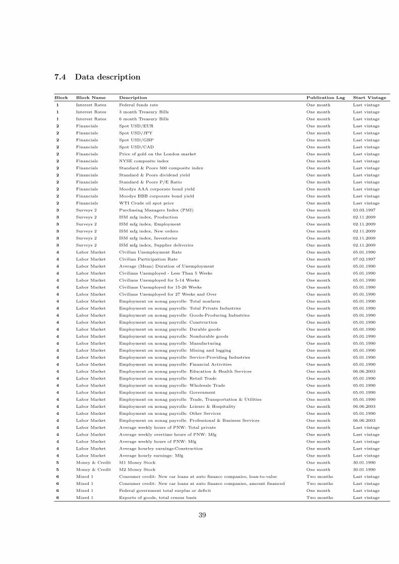
7.4 Data description
Block Block Name Description Publication Lag Start Vintage
1 Interest Rates Federal funds rate One month Last vintage
1 Interest Rates 3 month Treasury Bills One month Last vintage
1 Interest Rates 6 month Treasury Bills One month Last vintage
2 Financials Spot USD/EUR One month Last vintage
2 Financials Spot USD/JPY One month Last vintage
2 Financials Spot USD/GBP One month Last vintage
2 Financials Spot USD/CAD One month Last vintage
2 Financials Price of gold on the London market One month Last vintage
2 Financials NYSE composite index One month Last vintage
2 Financials Standard & Poors 500 composite index One month Last vintage
2 Financials Standard & Poors dividend yield One month Last vintage
2 Financials Standard & Poors P/E Ratio One month Last vintage
2 Financials Moodys AAA corporate bond yield One month Last vintage
2 Financials Moodys BBB corporate bond yield One month Last vintage
2 Financials WTI Crude oil spot price One month Last vintage
3 Surveys 2 Purchasing Managers Index (PMI) One month 03.03.1997
3 Surveys 2 ISM mfg index, Production One month 02.11.2009
3 Surveys 2 ISM mfg index, Employment One month 02.11.2009
3 Surveys 2 ISM mfg index, New orders One month 02.11.2009
3 Surveys 2 ISM mfg index, Inventories One month 02.11.2009
3 Surveys 2 ISM mfg index, Supplier deliveries One month 02.11.2009
4 Labor Market Civilian Unemployment Rate One month 05.01.1990
4 Labor Market Civilian Participation Rate One month 07.02.1997
4 Labor Market Average (Mean) Duration of Unemployment One month 05.01.1990
4 Labor Market Civilians Unemployed - Less Than 5 Weeks One month 05.01.1990
4 Labor Market Civilians Unemployed for 5-14 Weeks One month 05.01.1990
4 Labor Market Civilians Unemployed for 15-26 Weeks One month 05.01.1990
4 Labor Market Civilians Unemployed for 27 Weeks and Over One month 05.01.1990
4 Labor Market Employment on nonag payrolls: Total nonfarm One month 05.01.1990
4 Labor Market Employment on nonag payrolls: Total Private Industries One month 05.01.1990
4 Labor Market Employment on nonag payrolls: Goods-Producing Industries One month 05.01.1990
4 Labor Market Employment on nonag payrolls: Construction One month 05.01.1990
4 Labor Market Employment on nonag payrolls: Durable goods One month 05.01.1990
4 Labor Market Employment on nonag payrolls: Nondurable goods One month 05.01.1990
4 Labor Market Employment on nonag payrolls: Manufacturing One month 05.01.1990
4 Labor Market Employment on nonag payrolls: Mining and logging One month 05.01.1990
4 Labor Market Employment on nonag payrolls: Service-Providing Industries One month 05.01.1990
4 Labor Market Employment on nonag payrolls: Financial Activities One month 05.01.1990
4 Labor Market Employment on nonag payrolls: Education & Health Services One month 06.06.2003
4 Labor Market Employment on nonag payrolls: Retail Trade One month 05.01.1990
4 Labor Market Employment on nonag payrolls: Wholesale Trade One month 05.01.1990
4 Labor Market Employment on nonag payrolls: Government One month 05.01.1990
4 Labor Market Employment on nonag payrolls: Trade, Transportation & Utilities One month 05.01.1990
4 Labor Market Employment on nonag payrolls: Leisure & Hospitality One month 06.06.2003
4 Labor Market Employment on nonag payrolls: Other Services One month 05.01.1990
4 Labor Market Employment on nonag payrolls: Professional & Business Services One month 06.06.2003
4 Labor Market Average weekly hours of PNW: Total private One month Last vintage
4 Labor Market Average weekly overtime hours of PNW: Mfg One month Last vintage
4 Labor Market Average weekly hours of PNW: Mfg One month Last vintage
4 Labor Market Average hourley earnings:Construction One month Last vintage
4 Labor Market Average hourly earnings: Mfg One month Last vintage
5 Money & Credit M1 Money Stock One month 30.01.1990
5 Money & Credit M2 Money Stock One month 30.01.1990
6 Mixed 1 Consumer credit: New car loans at auto finance companies, loan-to-value Two months Last vintage
6 Mixed 1 Consumer credit: New car loans at auto finance companies, amount financed Two months Last vintage
6 Mixed 1 Federal government total surplus or deficit One month Last vintage
6 Mixed 1 Exports of goods, total census basis Two months Last vintage
39
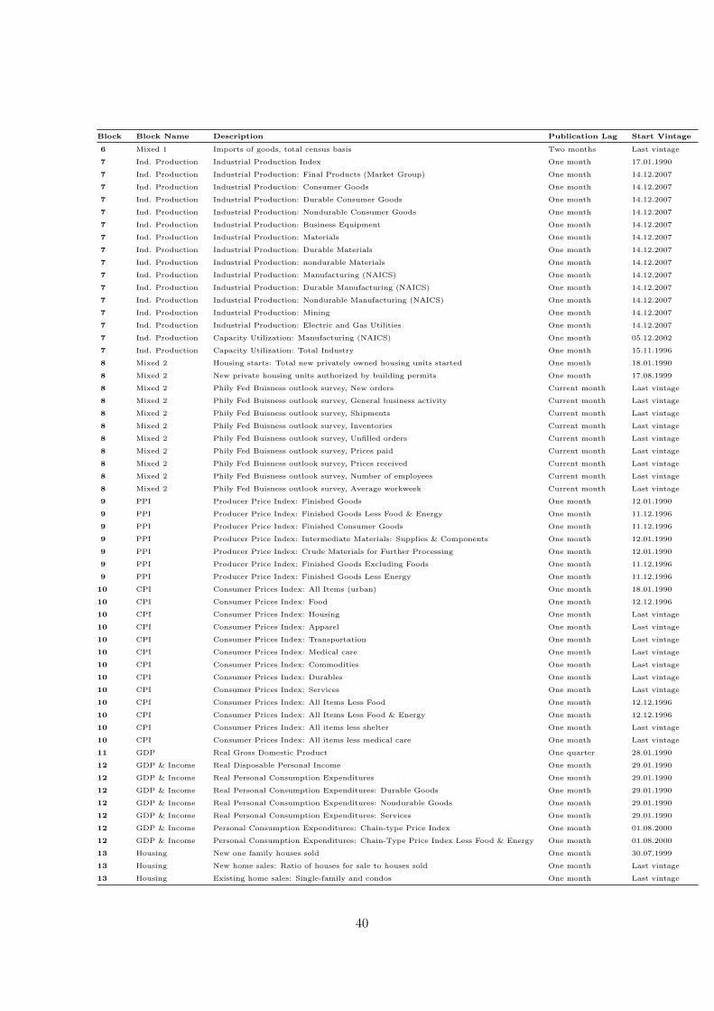
Block Block Name Description Publication Lag Start Vintage
6 Mixed 1 Imports of goods, total census basis Two months Last vintage
7 Ind. Production Industrial Production Index One month 17.01.1990
7 Ind. Production Industrial Production: Final Products (Market Group) One month 14.12.2007
7 Ind. Production Industrial Production: Consumer Goods One month 14.12.2007
7 Ind. Production Industrial Production: Durable Consumer Goods One month 14.12.2007
7 Ind. Production Industrial Production: Nondurable Consumer Goods One month 14.12.2007
7 Ind. Production Industrial Production: Business Equipment One month 14.12.2007
7 Ind. Production Industrial Production: Materials One month 14.12.2007
7 Ind. Production Industrial Production: Durable Materials One month 14.12.2007
7 Ind. Production Industrial Production: nondurable Materials One month 14.12.2007
7 Ind. Production Industrial Production: Manufacturing (NAICS) One month 14.12.2007
7 Ind. Production Industrial Production: Durable Manufacturing (NAICS) One month 14.12.2007
7 Ind. Production Industrial Production: Nondurable Manufacturing (NAICS) One month 14.12.2007
7 Ind. Production Industrial Production: Mining One month 14.12.2007
7 Ind. Production Industrial Production: Electric and Gas Utilities One month 14.12.2007
7 Ind. Production Capacity Utilization: Manufacturing (NAICS) One month 05.12.2002
7 Ind. Production Capacity Utilization: Total Industry One month 15.11.1996
8 Mixed 2 Housing starts: Total new privately owned housing units started One month 18.01.1990
8 Mixed 2 New private housing units authorized by building permits One month 17.08.1999
8 Mixed 2 Phily Fed Buisness outlook survey, New orders Current month Last vintage
8 Mixed 2 Phily Fed Buisness outlook survey, General business activity Current month Last vintage
8 Mixed 2 Phily Fed Buisness outlook survey, Shipments Current month Last vintage
8 Mixed 2 Phily Fed Buisness outlook survey, Inventories Current month Last vintage
8 Mixed 2 Phily Fed Buisness outlook survey, Unfilled orders Current month Last vintage
8 Mixed 2 Phily Fed Buisness outlook survey, Prices paid Current month Last vintage
8 Mixed 2 Phily Fed Buisness outlook survey, Prices received Current month Last vintage
8 Mixed 2 Phily Fed Buisness outlook survey, Number of employees Current month Last vintage
8 Mixed 2 Phily Fed Buisness outlook survey, Average workweek Current month Last vintage
9 PPI Producer Price Index: Finished Goods One month 12.01.1990
9 PPI Producer Price Index: Finished Goods Less Food & Energy One month 11.12.1996
9 PPI Producer Price Index: Finished Consumer Goods One month 11.12.1996
9 PPI Producer Price Index: Intermediate Materials: Supplies & Components One month 12.01.1990
9 PPI Producer Price Index: Crude Materials for Further Processing One month 12.01.1990
9 PPI Producer Price Index: Finished Goods Excluding Foods One month 11.12.1996
9 PPI Producer Price Index: Finished Goods Less Energy One month 11.12.1996
10 CPI Consumer Prices Index: All Items (urban) One month 18.01.1990
10 CPI Consumer Prices Index: Food One month 12.12.1996
10 CPI Consumer Prices Index: Housing One month Last vintage
10 CPI Consumer Prices Index: Apparel One month Last vintage
10 CPI Consumer Prices Index: Transportation One month Last vintage
10 CPI Consumer Prices Index: Medical care One month Last vintage
10 CPI Consumer Prices Index: Commodities One month Last vintage
10 CPI Consumer Prices Index: Durables One month Last vintage
10 CPI Consumer Prices Index: Services One month Last vintage
10 CPI Consumer Prices Index: All Items Less Food One month 12.12.1996
10 CPI Consumer Prices Index: All Items Less Food & Energy One month 12.12.1996
10 CPI Consumer Prices Index: All items less shelter One month Last vintage
10 CPI Consumer Prices Index: All items less medical care One month Last vintage
11 GDP Real Gross Domestic Product One quarter 28.01.1990
12 GDP & Income Real Disposable Personal Income One month 29.01.1990
12 GDP & Income Real Personal Consumption Expenditures One month 29.01.1990
12 GDP & Income Real Personal Consumption Expenditures: Durable Goods One month 29.01.1990
12 GDP & Income Real Personal Consumption Expenditures: Nondurable Goods One month 29.01.1990
12 GDP & Income Real Personal Consumption Expenditures: Services One month 29.01.1990
12 GDP & Income Personal Consumption Expenditures: Chain-type Price Index One month 01.08.2000
12 GDP & Income Personal Consumption Expenditures: Chain-Type Price Index Less Food & Energy One month 01.08.2000
13 Housing New one family houses sold One month 30.07.1999
13 Housing New home sales: Ratio of houses for sale to houses sold One month Last vintage
13 Housing Existing home sales: Single-family and condos One month Last vintage
40

Block Block Name Description Publication Lag Start Vintage
14 Surveys 1 Chicago Fed MMI Survey One month Last vintage
14 Surveys 1 Composite index of 10 leading indicators One month Last vintage
14 Surveys 1 Consumer confidence surveys: Index of consumer confidence Current month Last vintage
14 Surveys 1 Michigan Survey: Index of consumer sentiment Current month 31.07.1998
15 Initial Claims Average weekly initial claims Current month Last vintage
41

Centre for Applied Macro - and Petroleum economics (CAMP) The objective of CAMP is to provide high quality research and analysis into the field of macroeconomics, as well as financial issues.
The research activities of CAMP will be broad and will encompass all elements pertaining to the analysis of macroeconomic data.
Bi Norwegian Business SchoolCentre for Applied Macro - Petroleum economics (CAMP)N-0442 oslo
http://www.bi.no/camp
CAMP Working Paper SeriesiSSN: 1893-4811
CeNTre for APPlieD MACro - AND PeTroleUM eCoNoMiCS (CAMP)