GEE for Longitudinal Data

² GEE: generalized estimating equationsLiang & Zeger, 1986; Zeger & Liang, 1986

² extension of quasi-likelihood to longitudinal data analysis

² method is semi-parametric

{ estimating equations are derived without fullspeci¯cation of the joint distribution of a subject'sobservations

² instead, speci¯cation of

{ likelihood for the (univariate) marginal distributions

{ \working" covariance matrix for the vector orrepeated observations from each subject

² Dunlop (1994) American Statistician

² Diggle, Liang, & Zeger (1994) Analysis of LongitudinalData, chapters 7 & 8

1

GEE overview

² GEEs have consistent and asymptotically normalsolutions, even with mis-speci¯cation of the correlationstructure

² Avoids need for multivariate distributions by onlyassuming a functional form for the marginal distributionat each timepoint

² The covariance structure is treated as a nuisance

² Relies on the independence across subjects to estimateconsistently the variance of the regression coe±cients(even when the assumed correlation structure isincorrect)

2

GEE Method outline

1. Relate the marginal response ¹ij = E(yij) to a linearcombination of the covariates

g(¹ij) = xij ¯

² yij is the response for subject i at time j

² xij is a p£ 1 vector of covariates

² ¯ is a p£ 1 vector or unknown regression coe±cients

² g(¢) is the link function

2. Describe the variance of yij as a function of the mean

V (yij) = V (¹ij) Á

² Á is a possibly unknown scale parameter

² V (¢) is the variance function

3

Link and Variance Functions

Normally-distributed response

g(¹ij) = ¹ij \Identity link"

V (¹ij) = 1

V (yij) = Á

Binary response

g(¹ij) = log[¹ij=(1¡ ¹ij)] \Logit link"

V (¹ij) = ¹ij (1¡ ¹ij)

Á = 1

Poisson response

g(¹ij) = log(¹ij) \Logarithm link"

V (¹ij) = ¹ij

Á = 1

4

GEE method outline

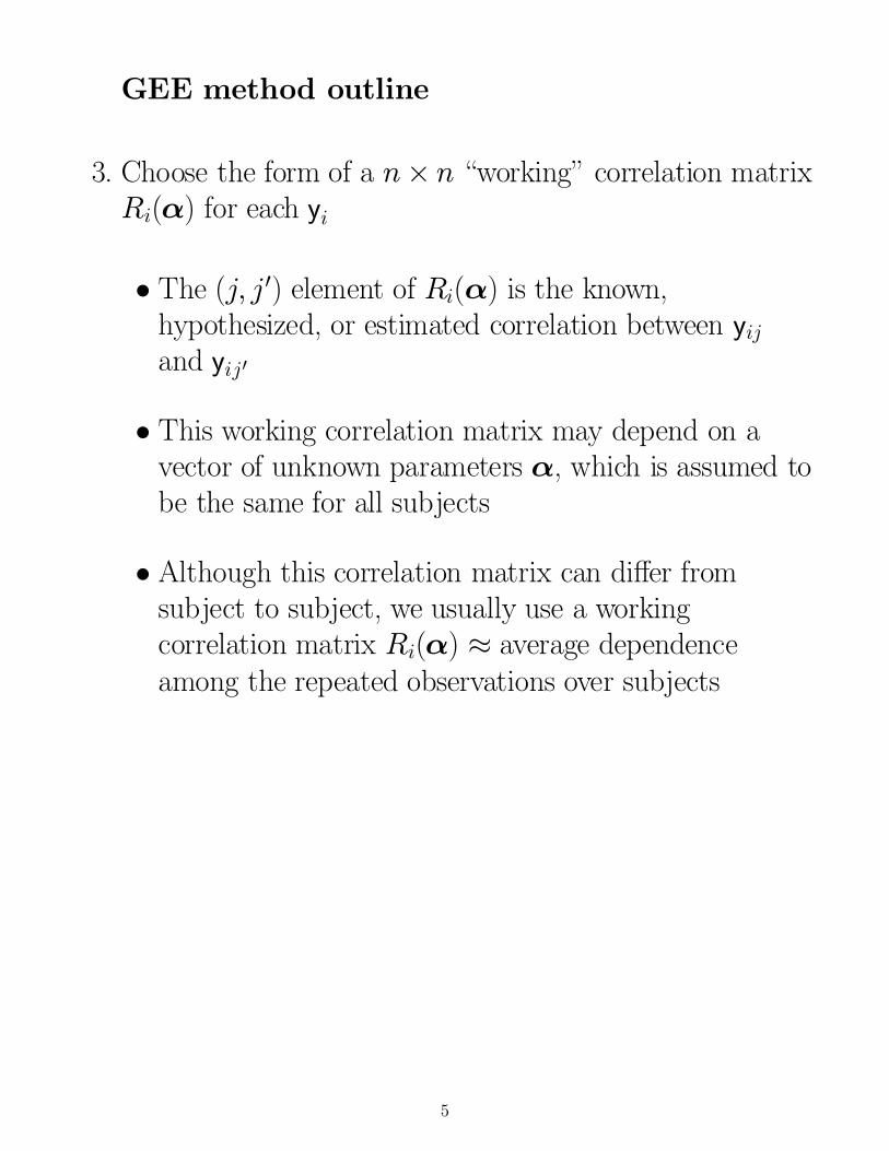
3. Choose the form of a n£ n \working" correlation matrixRi(®) for each yi

² The (j; j 0) element of Ri(®) is the known,hypothesized, or estimated correlation between yijand yij0

² This working correlation matrix may depend on avector of unknown parameters ®, which is assumed tobe the same for all subjects

² Although this correlation matrix can di®er fromsubject to subject, we usually use a workingcorrelation matrix Ri(®) ¼ average dependenceamong the repeated observations over subjects

5

Comments on \working" correlation matrix

² should choose form of R to be consistent with empiricalcorrelations

² GEE method yields consistent estimates of regressioncoe±cients and their variances, even withmis-speci¯cation of the structure of the covariance matrix

² Loss of e±ciency from an incorrect choice of R islessened as the number of subjects gets large

6

Working correlation structures

² Exchangeable: Rjj0 = ®

{ same structure as in random-intercepts model

² AR(1): Rjj0 = ®jj¡j0j

² Stationary m-dependent (Toeplitz)

Rjj0 =

8>>><>>>:

®jtj¡tj0 j if jtj ¡ tj0j · m

0 if jtj ¡ tj0j > m

where tij is the jth observed timepoint

² Unspeci¯ed Rjj0 = ®jj0

{ n(n¡ 1)=2 parameters to be estimated

{ most e±cient, but useful only when there arerelatively few observations

{ missing data complicates estimation of R

{ the estimate obtained using nonmissing data is notguaranteed to be positive de¯nite

x0Rx > 0 for all x 6= 0

) problematic inversion of R

7

Generalized Estimating Equation

² Ai = n £ n diagonal matrix with V (¹ij) as the jthdiagonal element

{ for normal case, Ai = I i

² Ri(®) = n£ n \working" correlation matrix for ithsubject

² Working covariance matrix for yi

Vi(®) = ÁA1=2i Ri(®)A1=2

i

{ for normal case,

Vi(®) = ÁRi(®)

{ Note: Park (1993) extends this to heterogeneous scaleparameter Áj across time (j = 1; : : : ; n)

8

GEE estimate of ¯ is the solution of

NX

i=1D0

i [Vi(®)]¡1 (yi ¡ ¹i) = 0

where ® is a consistent estimate of ® and Di = @¹i=@¯

Normal case

¹i = Xi¯

Di = Xi

Vi(®) = Ri(®)

Thus,

NX

i=1X0

i [Ri(®)]¡1 (yi ¡Xi¯) = 0

and solving for ¯ yields

^ =8><>:

NX

i=1X0

i [Ri(®)]¡1Xi

9>=>;

¡1 8><>:

NX

i=1X0

i [Ri(®)]¡1 yi

9>=>;

) WLS estimate

9

Solving the GEE

Iterate between quasi-likelihood methods for estimating ¯and a robust method for estimating ® as a function of ¯

1. Given current estimates of Ri(®) and Á! calculate updated estimate of ¯ using iterativelyreweighted LS

2. Given the estimate of ¯! Pearson (or standardized) residuals

rij = (yij ¡ ¹ij)=s

[Vi]jj

note: in normal case denominator = 1

3. Use residuals rij to consistently estimate ®(see Liang & Zeger, 1986)

4. Repeat 1-3 until convergence

10

V ( ^ ): square root of diagonal elements yield standard errorsfor regression coe±cients

1. naive or \model-based"

V ( ^ ) = ¾2264NX

i=1D0

iV¡1i Di

375

¡1

2. robust or \empirical"

V ( ^ ) = M¡10 M 1M

¡10

where

M0 =NX

i=1D0

iV¡1i Di

M1 =NX

i=1D0

i(yi ¡ ¹i)(yi ¡ ¹i)0V ¡1i Di

² consistent estimator of V ( ^ ) even when

{ V (yij) 6= ÁV (¹ij) or when

{ Ri(®) is not the correlation matrix of yi

) Notice, if ¾2Vi = (yi ¡ ¹i)(yi ¡ ¹i)0, then two equationsare the same

11

GEE vs MRM

² GEE not concerned with structure of V (yi)\sweeps this mess under the table"

² GEE computes both a robust and a model-basedestimate of V (¯), MRM only computes model-based

² GEE can be used to ¯t Poisson or binomial data as well;more work, but MRM can be derived for Poisson orbinomial

² GEE assumption regarding missing data: MCARMRM assumption regarding missing data: MAR

{ MCAR: missing data are random conditional oncovariates

{ MAR: missing data are random conditional oncovariates and observed values of the dependentvariable

² Interpretation of ¯ di®ers for non-normal outcomes

{ population-averaged for GEE (marginal)

{ subject-speci¯c for MRM (conditional)

12

GEE Example: Smoking Cessation across Time

Gruder, Mermelstein, et al., (1993)Journal of Consulting & Clinical Psychology

² 489 subjects measures across 4 timepoints following anintervention designed to help them quit smoking

² Subject were randomized to one of three conditions

{ control - self help manuals

{ tx1 - group meetings

{ tx2 - enhanced group meetings

² Some subjects randomized to tx1 or tx2 never showed upto any meetings following the phone call informing themof where the meetings would take place

² In analysis, we focused on 4 groups using Helmertcontrasts to test for between-group e®ects

group h1 h2 h3control -1 0 0

no-shows 1/3 -1 0tx1 1/3 1/2 -1tx2 1/3 1/2 1

13

Interpretation of Helmert Contrasts

group h1 h2 h3control -1 0 0

no-shows 1/3 -1 0tx1 1/3 1/2 -1tx2 1/3 1/2 1

h1 test of whether randomization to group in°uencedsubsequent cessation rates

h2 test of whether showing up to the group meetingsin°uenced subsequent cessation

h3 test of whether type of meeting in°uenced cessation

Note: h1 is experimental comparison, however h2 and h3 arequasi-experimental comparisons

Examination for Possible Confounders

Baseline analysis indicated that groups di®ered in terms ofrace (w vs nw), so race was included in all subsequentanalyses involving group

14

15

16

17

Gruder, Mermelstein et al., (1993) Data (N = 489 andPN ni = 1744)

Smoking Status (smoking=0 and quit=1) across Time (4 timepoints)

Logistic Regression Model Estimates (standard errors)

ML models GEE models

Model terms independent independent exchange exchange

intercept -1.148 -1.175 -1.148 -1.172

¯0 (.098) (.103) (.109) (.114)

linear trend (0,1,2,3) -0.175 -0.155 -0.167 -0.147

¯1 (.054) (.056) (.051) (.054)

Tx vs. Control (H1) 0.484 0.801 0.523 0.798

¯2 (.121) (.194) (.169) (.221)

Groups vs. No-Show (H2) 0.255 0.356 0.253 0.348

¯3 (.090) (.136) (.120) (.144)

Enhanced vs. Usual (H3) 0.194 0.283 0.199 0.278

¯4 (.088) (.136) (.120) (.144)

Race (0=nw 1=w) 0.426 0.423 0.396 0.395

¯5 (.140) (.140) (.196) (.197)

H1 by Time -0.239 -0.235

¯6 (.108) (.104)

H2 by Time -0.079 -0.082

¯7 (.080) (.075)

H3 by Time -0.068 -0.067

¯8 (.081) (.078)

18

Gruder, Mermelstein et al., (1993) Data (N = 489 andPN ni = 1744)

Smoking Status (smoking=0 and quit=1) across Time (4 timepoints)

GEE Logistic Regression Model Estimates (standard errors)

Model terms exchange AR(1) m-depend UN

intercept -1.172 -1.073 -1.143 -1.167

¯0 (.114) (.113) (.114) (.114)

linear trend (0,1,2,3) -0.147 -0.170 -0.152 -0.139

¯1 (.054) (.053) (.054) (.054)

Tx vs. Control (H1) 0.798 0.788 0.796 0.804

¯2 (.221) (.214) (.219) (.221)

Groups vs. No-Show (H2) 0.348 0.388 0.358 0.345

¯3 (.144) (.145) (.144) (.144)

Enhanced vs. Usual (H3) 0.278 0.288 0.280 0.277

¯4 (.144) (.144) (.144) (.144)

Race (0=nw 1=w) 0.395 0.350 0.378 0.371

¯5 (.197) (.198) (.196) (.197)

H1 by Time -0.235 -0.236 -0.236 -0.233

¯6 (.104) (.099) (.103) (.104)

H2 by Time -0.082 -0.087 -0.083 -0.076

¯7 (.075) (.075) (.075) (.074)

H3 by Time -0.067 -0.069 -0.068 -0.067

¯8 (.078) (.077) (.078) (.077)

19

GEE example: comparison with MRMRiesby data - dichotomized response across time

20

21

22

23

Riesby Data - analysis of dichotomized HDRS

1. Logistic regression

log

26664

P (respij)

1¡P (respij)

37775 = ¯0 + ¯1Weekij + ¯2DMIij

2. GEE logistic regression with exchangeable correlations

log

26664P (respij)

1¡P (respij)

37775 = ¯0 + ¯1Weekij + ¯2DMIij

3. Random-intercepts logistic regression

log

26664P (respij)

1¡ P (respij)

37775 = ¯0 + ¯1Weekij + ¯2DMIij + ¾Àµi

µi » N (0; 1)

µi = subject e®ect (random) on log odds or response

¾2À = population variance of (random) subject e®ects

i = 1; : : : ; 66 subjects

j = 1; : : : ; ni obs per subject (max ni = 4)

Week = [ 0 1 2 3 ]

DMI =

8><>:

0 below median

1 above median

24

Riesby Data (N = 66 and PNi ni = 250) - last 4 weeks

LR analysis of dichotomous HRDS (· 15 vs > 15)Model estimates (standard errors)

model term ordinary LR GEE exchange Random Int

intercept ¯0 -.339 -.397 -.661(.182) (.231) (.407)

exp(¯0) .712 .672 .516

DMI ¯1 .985 1.092 1.8421=high, 0=low (.262) (.319) (.508)

exp(¯1) 2.68 2.98 6.31

subject sd ¾À 2.004(.415)

intra-subj corr .55

25

Riesby Data (N = 66 and PNi ni = 250) - last 4 weeks

LR analysis of dichotomous HRDS (· 15 vs > 15)Model estimates, standard errors, z-values, and exp( ^) forDichotomized Ln DMI e®ect (median & mean cut at 4.7)

model ^ se( ^) z exp( ^)ordinary LRint + DMI .985 .252 3.77 2.68int + time + DMI .911 .272 3.35 2.49

GEE LR - exchangeable working correlationint + DMI 1.092 .319 3.42 2.98int + time + DMI .851 .326 2.61 2.34

GEE LR - AR(1) working correlationint + DMI 1.058 .308 3.44 2.88int + time + DMI .914 .315 2.90 2.50

random intercepts LRint + DMI 1.842 .508 3.63 6.31int + time + DMI 1.813 .678 2.68 6.13

random intercepts & time trend LRint + time + DMI 2.450 1.012 2.42 11.59

26

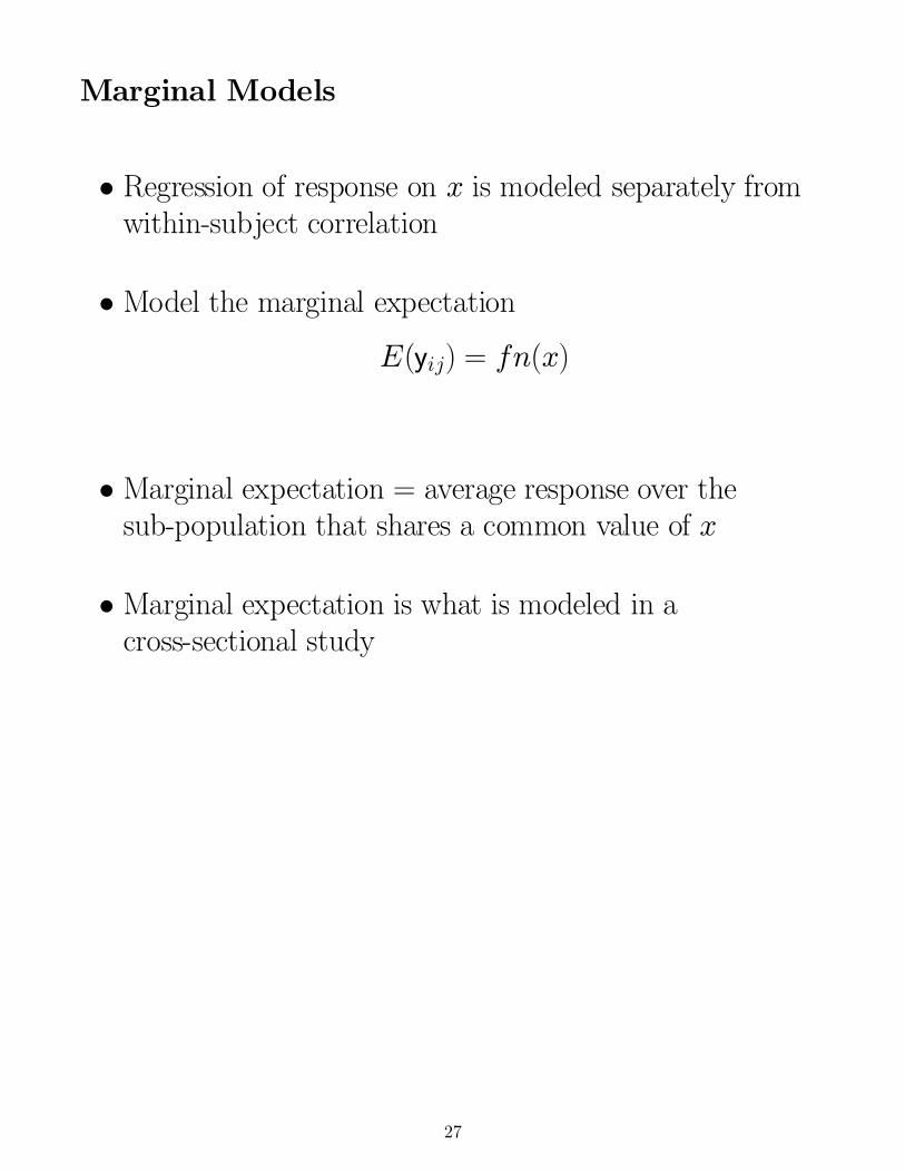
Marginal Models

² Regression of response on x is modeled separately fromwithin-subject correlation

² Model the marginal expectation

E(yij) = fn(x)

² Marginal expectation = average response over thesub-population that shares a common value of x

² Marginal expectation is what is modeled in across-sectional study

27

Assumptions of Marginal Model

1. Marginal expectation of the response E(yij) = ¹ijdepends on xij through link function g(¹ij)

e.g., logit link for binary responses

2. Marginal variance depends on marginal mean

V (yij) = V (¹ij)Á

² V = known variance function

² Á = scale parameter

3. Correlation between yij and yij0 is a function of themarginal means and/or parameters ®

) Marginal regression coe±cients have the sameinterpretation as coe±cients from a cross-sectional analysis

28

Logistic GEE as marginal model: Riesby example

yij =

8>><>>:

0 no response from depression1 response from depression

xij =

8>><>>:

0 ln DMI below marginal median 4.71 ln DMI above marginal median 4.7

1. logit(¹ij) = ln24 ¹ij1¡¹ij

35

= ln

2664P (yij = 1)

1¡ P (yij = 1)

3775 = ¯0 + ¯1xij

2. V (yij) = ¹ij(1¡ ¹ij)

3. Corr(yij ; yij0) = exchangeable, or AR, or : : :

29

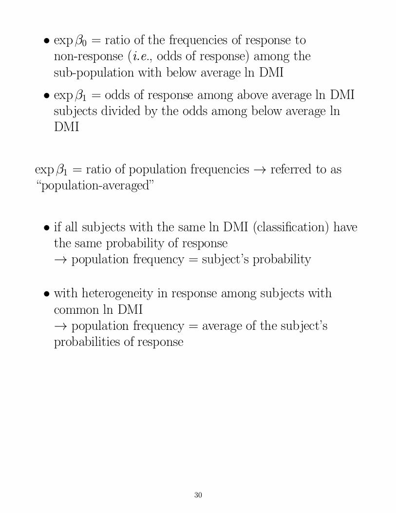
² exp¯0 = ratio of the frequencies of response tonon-response (i.e., odds of response) among thesub-population with below average ln DMI

² exp¯1 = odds of response among above average ln DMIsubjects divided by the odds among below average lnDMI

exp¯1 = ratio of population frequencies ! referred to as\population-averaged"

² if all subjects with the same ln DMI (classi¯cation) havethe same probability of response! population frequency = subject's probability

² with heterogeneity in response among subjects withcommon ln DMI! population frequency = average of the subject'sprobabilities of response

30

Random intercepts logistic regression

P (yij = 1 j Ài) =½1 + exp[¡(x0ij¯ + Ài)]

¾¡1

P (yij = 0 j Ài) = 1¡ P (yij = 1 j Ài)

ln

2664P (yij = 1 j Ài)P (yij = 0 j Ài)

3775 = ln

2664

1

1 + exp(¡z)£ 1

1¡ [1=(1 + exp(¡z))]

3775

= ln [1=(1 + exp(¡z)¡ 1)]

= x0ij¯ + Ài

g (P (yij = 1 j Ài)) = x0ij¯ + Ài

P (yij = 1 j Ài) = g¡1µx0ij¯ + Ài

¶

where g is the logit link function. Notice

E(yij j Ài) = g¡1µx0ij¯ + Ài

¶

¹ij = E(yij) = E [E(yij j Ài)] =Z

À g¡1

µx0ij¯ + Ài

¶dF (Ài)

where F (Ài) represents the population distribution of Ài

31

With Ài » N(0; ¾2À), we can standardize the random-e®ect

distribution,

µi =Ài¾À

! Ài = µi¾À

and so,

¹ij = E(yij) =Z

µ g¡1

µx0ij¯ + ¾Àµi

¶f(µi)dµ

where µi » N (0; 1).

Note in terms of the vector response,

¹i = E(yi) =Z

µ

264niY

j=1g¡1

µx0ij¯ + ¾Àµi

¶375 f (µi)dµ

When g is a non-linear function and if we assume that

g(¹ij) = x0ij¯ + ¾Àµi

it is usually not true that

g(¹ij) = x0ij¯

unless

² Ài = 0 8i² g is the identity link (normal y regression)

) ¯ss 6= ¯pa

32

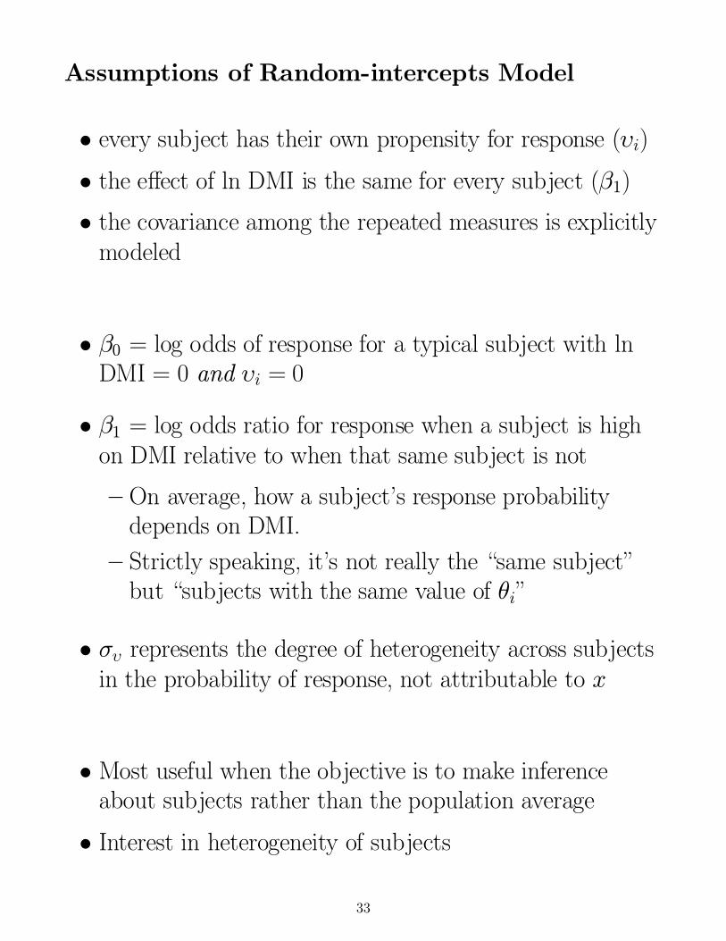
Assumptions of Random-intercepts Model

² every subject has their own propensity for response (Ài)

² the e®ect of ln DMI is the same for every subject (¯1)

² the covariance among the repeated measures is explicitlymodeled

² ¯0 = log odds of response for a typical subject with lnDMI = 0 and Ài = 0

² ¯1 = log odds ratio for response when a subject is highon DMI relative to when that same subject is not

{ On average, how a subject's response probabilitydepends on DMI.

{ Strictly speaking, it's not really the \same subject"but \subjects with the same value of µi"

² ¾À represents the degree of heterogeneity across subjectsin the probability of response, not attributable to x

² Most useful when the objective is to make inferenceabout subjects rather than the population average

² Interest in heterogeneity of subjects

33

Random-intercepts Model with time-invariantcovariate (xi)

ln

2664P (yij = 1 j Ài)P (yij = 0 j Ài)

3775 = ¯0 + ¯1xi + Ài

where xi =

8>><>>:

0 control grp1 treatment grp

² ¯0 = log odds of response for a control subject withÀi = 0

² ¯1 = log odds ratio for response when a subject is\treated" relative to when that same subject (or really,subject with the same value of Ài) is \control"

In some sense, interpretation of ¯1 goes beyond the observeddata

34

Interpretation of regression coe±cients

mixed models ¯ represent the e®ects of the explanatoryvariables on a subject's chance of response(subject-speci¯c)

marginal models ¯ represents the e®ects of theexplanatory variables on the population average(population-averaged)

Odds Ratio

mixed models describes the ratio of a subject's odds

marginal models describes the ratio of the populationodds

Neuhaus et al., 1991

² if ¾2À > 0 ) j ¯ss j > j ¯pa j

² discrepancy increases as ¾2À increases (unless ¯ss = 0,

then ¯pa = 0)

35

Comparing Fixed to Mixed-e®ects LR

Fixed-e®ects Logistic Regression

yij = x0ij¯f + "ij

"ij » L(0; ¼2=3)

! V (yij) = ¼2=3

Random intercepts Logistic Regression

yij = x0ij¯r + Ài + "ij

Ài » N(0; ¾2À)

"ij » L(0; ¼2=3)

! V (yij) = ¼2=3 + ¾2À

) suggests that to equate

¯f ¼ ¯r=

vuuuuut¼2=3 + ¾2

À

¼2=3= ¯r=

vuuuut3

¼2¾2À + 1

Zeger et al., 1988 suggests a slightly larger denominator

¯f ¼ ¯r=

vuuuuut

0B@16

15

1CA

2 3

¼2¾2À + 1

36

HDRS response probability by DMI median cutsubjects with varying DMI values across time (n = 20)

P (respij = 1) = 1= [1 + exp(¡(¯0 + ¯1DMIij + Ài))]

^0 = ¡:66 ^

1 = 1:84 exp( ^1) = 6:31 ¾À = 2:00

From GEE analysis with exchangeable working correlation^0 = ¡:40 ^

1 = 1:09 exp( ^1) = 2:98

px=0 = :40 px=1 = :67

37

HDRS response probability by DMI median cutsubjects with consistent DMI values across time(low DMI: n = 24, high DMI: n = 22)

P (respij = 1) = 1= [1 + exp(¡(¯0 + ¯1DMIij + Ài))]

^0 = ¡:66 ^

1 = 1:84 exp( ^1) = 6:31 ¾À = 2:00

From GEE analysis with exchangeable working correlation^0 = ¡:40 ^

1 = 1:09 exp( ^1) = 2:98

px=0 = :40 px=1 = :67

38

TITLE1 'Riesby Data - Estimated Marginal Probabilities';

PROC IML;

/* covariate matrix for low drug level observations */

x0 = f 1 0g;/* covariate matrix for high drug level observations */

x1 = f 1 1g;

/* GEE analysis - exchangeable working correlation */

beta = f-0.397, 1.092g;z0 = x0*beta; z1 = x1*beta;

mprb0 = 1.0 / (1.0 + EXP(0 - z0));

mprb1 = 1.0 / (1.0 + EXP(0 - z1));

print 'GEE ANALYSIS - exchangeable working correlation';

print 'marginal prob for low drug', mprb0 [FORMAT=8.4];

print 'marginal prob for high drug',mprb1 [FORMAT=8.4];

GEE ANALYSIS - exchangeable working correlation

marginal prob for low drug

MPRB0

0.4020

marginal prob for high drug

MPRB1

0.6671

39

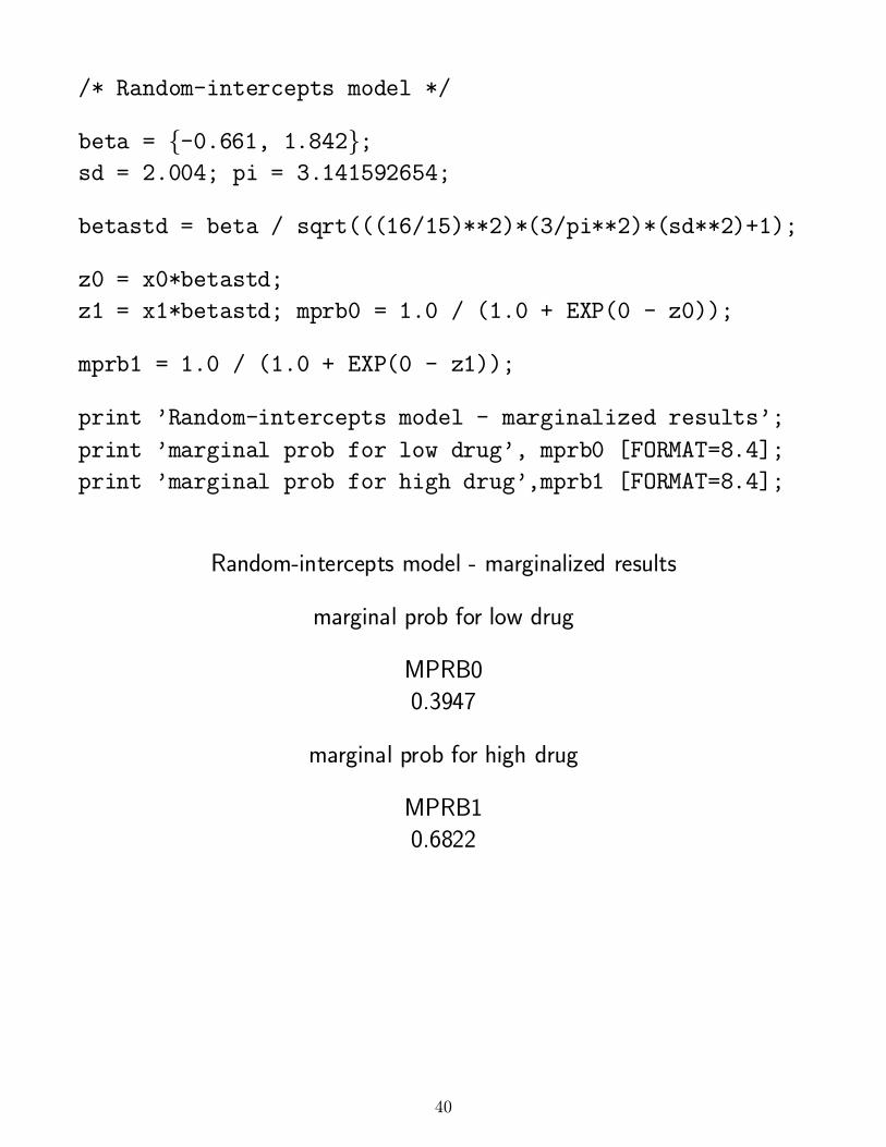
/* Random-intercepts model */

beta = f-0.661, 1.842g;sd = 2.004; pi = 3.141592654;

betastd = beta / sqrt(((16/15)**2)*(3/pi**2)*(sd**2)+1);

z0 = x0*betastd;

z1 = x1*betastd; mprb0 = 1.0 / (1.0 + EXP(0 - z0));

mprb1 = 1.0 / (1.0 + EXP(0 - z1));

print 'Random-intercepts model - marginalized results';

print 'marginal prob for low drug', mprb0 [FORMAT=8.4];

print 'marginal prob for high drug',mprb1 [FORMAT=8.4];

Random-intercepts model - marginalized results

marginal prob for low drug

MPRB0

0.3947

marginal prob for high drug

MPRB1

0.6822

40

/* get the estimated marginal probs using quadrature */;

/* number of points, quadrature nodes & weights */;

nq = 10;

bq = f -4.85946282833231, -3.58182348355193,

-2.48432584163895, -1.46598909439116, -0.48493570751550,

0.48493570751550, 1.46598909439116, 2.48432584163895,

3.58182348355193, 4.85946282833231g;aq = f 0.00000431065265, 0.00075807095698,

0.01911158107317, 0.13548370704150, 0.34464234526294,

0.34464234526294, 0.13548370704150, 0.01911158107317,

0.00075807095698, 0.00000431065265g;

mprb0 = 0; mprb1 = 0;

DO q = 1 to nq;

z0 = sd*bq[q] + x0*beta; z1 = sd*bq[q] + x1*beta;

mprb0 = mprb0 + ( 1.0 / (1.0 + EXP(0 - z0)))*aq[q];

mprb1 = mprb1 + ( 1.0 / (1.0 + EXP(0 - z1)))*aq[q];

END;

print 'Random-int model: Quad method - 10 points';

print 'marginal prob for low drug', mprb0 [FORMAT=8.4];

print 'marginal prob for high drug',mprb1 [FORMAT=8.4];

Random-int model: Quad method - 10 points

marginal prob for low drug

MPRB0

0.4014

marginal prob for high drug

MPRB1

0.6726

41