Gender and Urban Form1

Stephen Sheppard Williams College

Alison Kraley

Williams College

October 2009 Please check with author before quoting

Abstract In this paper we focus attention on the increasing participation of women in the labor market, and the impact that this participation has on urban form. We emphasize the impact of gender on urban form – in particular the total amount of urban land use or urban footprint – because of its relevance to urban policy formation and contemporary concerns about urban expansion. We consider both simple first difference models of urban land use and cross-section models estimated using instrumental variable techniques. In general we find support for the theoretical predictions. An increase in the FLFPR is associated, ceteris paribus, with reduced urban land use.

1 This research would not have been possible without the generous support of the US National Science Foundation (award SES-0433278) and the research committee of the World Bank.

1

I. Introduction

The year 2008 has been identified by the UN Population Fund as the year in which half of the world’s

population could be said to live in urban areas. This closes a century in which the urban population

increased by more than ten fold. More alarming, in the view of some, is the observation that at current

growth rates the urban population in developing countries will double over the next 25 years.

Why should this be alarming? One answer is the tremendous resource requirements associated with

providing the new infrastructure and providing accommodation for this growing urban population. Data

from a sample of cities around the globe (and described more fully below) suggests that total urban land

use in cities is increasing at an annual rate of about 2.56%. This implies that total urban land cover on

earth will double in 27 years. Thus in less than three decades, if current trends continue, we will have to

build as many hectares of urban environment as humans collectively managed to construct in the several

thousand years since urban places began.

Policy makers and others are also concerned about the environmental impact of urban populations in

general and in particular the impact of the expanding urban “footprint” – or amount of land covered by

buildings, concrete, roadways, and other impervious surfaces that characterize the built environment.

Finally, we might be concerned about the changing nature of human society organized in these urban

communities, in which regular social interaction of rural, village and small-town life are replaced with the

social segregation or isolation of cities.

Whether these concerns are reasonable is, of course, debatable (or at least a matter for further empirical

investigation) but each of them are related in some way to the compactness of the urban form – the extent

to which the built environment constructed to accommodate the new urban population is extensive and

large in quantity or more modest, higher density, and more ‘compact’ (however this might be measured).

An urban area that generates less total urban cover for a given population will involve less extensive and

sprawling infrastructure requirements. Higher density building places more of the costs of urban

expansion on developers and the new residents and less on the overstretched and often under financed

public sector. Reduced urban footprints makes for more compact cities, and these may have reduced

environmental impacts both in terms of reduced use of open space as well as reduced energy use and

commuting (as argued by Newman and Kenworthy (1989) but challenged by Breheny (1995)). Finally,

urban expansion might lead to increased urban isolation and exclusion. This is argued with a variety of

2

anecdotal data by Power (2001), although recent research by Brueckner and Largey (2007) calls this

hypothesis into question.

In order to better anticipate the infrastructure investment that will be required as well as other social and

economic problems (if any), it is important to understand the forces that drive urban expansion and

determine the extent of urban land use. This should include the obvious factors suggested by economic

theory such as income, population, transportation costs, and the opportunity cost of urban land. It should

also include an exploration of social and economic forces whose role in determining urban form is less

widely appreciated.

In this paper we focus attention on one such factor: the increasing participation of women in the labor

market, and the impact that this participation has on urban form. We emphasize the impact of gender on

urban form – in particular the total amount of urban land use or urban footprint – because of its relevance

to urban policy formation and contemporary concerns about urban expansion. There are many issues that

are affected by the changing economic role of women and their (generally) increasing access to

employment in the economy. These concerns: income distribution, relative influence in household

decision making, or labor market discrimination, are not directly addressed. We take the female labor

force participation rate as exogenously determined by social and labor market conditions, and ask: what

impact do these changes have on total urban land use?

II. Simple Models of Gender and Urban Expansion

Interest in the differences between male and female workers in the context of an urban labor market goes

back at least to the seminal paper by White (1977) and perhaps even to some limited observations and

conjectures by Kain (1962). Most papers considering the issue deal with an important empirical

regularity: on average, women in the labor market experience shorter commutes than men. From this

starting point the analyses follow a variety of paths, ranging from a focus on job search and the labor

force participation decision (such as Ommeren, Reitveld and Nijkamp (1998)). Others continue a focus on

the locations where females are likely to find employment and explore some of the consequences for

urban land rents (such as Hotchkiss and White (1993)).

For the purposes of our analysis, the first difficulty we must confront is to separate the impact of female

labor force participation from the increase in household income that it might bring. The impact of

3

increasing household income on urban form is unambiguous and empirically validated in many studies,

among them Angel, Sheppard and Civco (2005) and Blomberg and Sheppard (2007). These studies all

suggest that increasing income is associated with increased urban land use, holding all other factors

constant. The elasticity of total urban land use with respect to income is estimated to be between 0.4 and

0.8.

Let us consider for the moment a world in which all households are identical and consist of two adults.

One of them is always employed and works in the city center. The other may or may not work, and if

employment is sought it may be located between the urban center and the urban periphery. If we hold

household income constant and imagine the household switching from a state in which one adult works to

a state in which both work, the impact is obviously identical to an increase in commuting costs for the

household. If the second workplace is more suburbanized, then the impact on transport costs may be quite

small, but it clearly constitutes an increase in transport costs (with no corresponding change in income or

other economic variables). In this world, the impact of increasing female labor force participation is clear.

Letting x represent the maximum extent of urban development and t represent the per unit distance cost

of transportation:

0x xFLFPR t∂ ∂

= <∂ ∂

The inequality in the expression has been established by several analysts in the context of a monocentric

model, notably Brueckner (1987).

Based on this, a simple model of urban land use would predict that an increase in the female labor force

participation rate would, ceteris paribus, be associated with reduced urban land use and more compact

cities. Note that even if this is found to be empirically valid, the claim does NOT imply a policy

conclusion that policies that increase FLFPR (such as improved educational opportunities) will

necessarily result in more compact cities, since these policies may also have impacts on transportation

costs, household incomes, or other variables whose net contribution to urban expansion may be

ambiguous.

4

III. Data In order to determine the impacts of the female labor force participation rate and other economic variables

on urban expansion we need to combine two types of data. First is the information required to measure the

expansion of urban land use, and second is information on the economic and policy conditions that

influence the pace of expansion so that we can test our models of urban expansion and determine the

quantitative and qualitative nature of the relationships. For the first we rely upon remotely sensed satellite

data and for the second we rely upon a variety of sources including data collected by field researchers

deployed to each city in our sample. We discuss each in turn below.

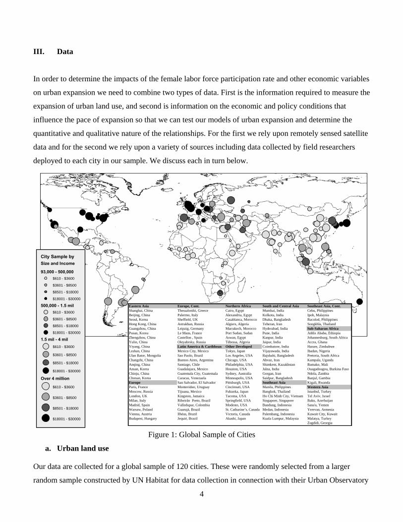
Figure 1: Global Sample of Cities

a. Urban land use Our data are collected for a global sample of 120 cities. These were randomly selected from a larger

random sample constructed by UN Habitat for data collection in connection with their Urban Observatory

Eastern Asia Europe, Cont. Northern Africa South and Central Asia Southeast Asia, Cont.Shanghai, China Thessaloniki, Greece Cairo, Egypt Mumbai, India Cebu, PhilippinesBeijing, China Palermo, Italy Alexandria, Egypt Kolkota, India Ipoh, MalaysiaSeoul, Korea Sheffield, UK Casablanca, Morocco Dhaka, Bangladesh Bacolod, PhilippinesHong Kong, China Astrakhan, Russia Algiers, Algeria Teheran, Iran Songkhla, ThailandGuangzhou, China Leipzig, Germany Marrakech, Morocco Hyderabad, India Sub-Saharan AfricaPusan, Korea Le Mans, France Port Sudan, Sudan Pune, India Addis Ababa, EthiopiaZhengzhou, China Castellon , Spain Aswan, Egypt Kanpur, India Johannesburg, South AfricaYulin, China Oktyabrsky, Russia Tébessa, Algeria Jaipur, India Accra, GhanaYiyang, China Latin America & Caribbean Other Developed Coimbatore, India Harare, ZimbabweLeshan, China Mexico City, Mexico Tokyo, Japan Vijayawada, India Ibadan, NigeriaUlan Bator, Mongolia Sao Paolo, Brazil Los Angeles, USA Rajshahi, Bangladesh Pretoria, South AfricaChangzhi, China Buenos Aires, Argentina Chicago, USA Ahvaz, Iran Kampala, UgandaAnqing, China Santiago, Chile Philadelphia, USA Shimkent, Kazakhstan Bamako, MaliAnsan, Korea Guadalajara, Mexico Houston, USA Jalna, India Ouagadougou, Burkina FasoChinju, China Guatemala City, Guatemala Sydney, Australia Gorgan, Iran Ndola, ZambiaChonan, Korea Caracas, Venezuela Minneapolis, USA Saidpur, Bangladesh Banjul, GambiaEurope San Salvador, El Salvador Pittsburgh, USA Southeast Asia Kigali, RwandaParis, France Montevideo, Uruguay Cincinnati, USA Manila, Philippines Western AsiaMoscow, Russia Tijuana, Mexico Fukuoka, Japan Bangkok, Thailand Istanbul, TurkeyLondon, UK Kingston, Jamaica Tacoma, USA Ho Chi Minh City, Vietnam Tel Aviv, IsraelMilan, Italy Ribeirão Preto, Brazil Springfield, USA Singapore, Singapore Baku, AzerbaijanMadrid, Spain Valledupar, Colombia Modesto, USA Bandung, Indonesia Sana'a, YemenWarsaw, Poland Guarujá, Brazil St. Catharine’s, Canada Medan, Indonesia Yerevan, ArmeniaVienna, Austria Ilhéus, Brazil Victoria, Canada Palembang, Indonesia Kuwait City, KuwaitBudapest, Hungary Jequié, Brazil Akashi, Japan Kuala Lumpur, Malaysia Malatya, Turkey

Zugdidi, Georgia

City Sample bySize and Income

93,000 - 500,000$610 - $3600

$3601 - $8500

$8501 - $18000

$18001 - $30000

500,000 - 1.5 mil$610 - $3600

$3601 - $8500

$8501 - $18000

$18001 - $30000

1.5 mil - 4 mil$610 - $3600

$3601 - $8500

$8501 - $18000

$18001 - $30000

Over 4 million

$610 - $3600

$3601 - $8500

$8501 - $18000

$18001 - $30000

5

program. The larger sample has been constructed to be representative of the global urban population in

cities having population over 100,000 persons. The figure below shows the location of each city, with

dots sized to indicate population and shaded to indicate per capita income. The table lists the cities by

global region.

Remotely sensed data

For each of the cities in our sample, we obtained Landsat thematic mapper satellite images for dates that

are relatively near the national census dates and for which cloud-free images are available. Images were

obtained for two time periods: approximately 1990 and approximately 2000. The actual image dates vary

and the sample mean time period between images is just over 11 years. The images themselves provide

data on reflected light intensity in 7 spectral bands (3 visual and 4 infrared). These data are used to

classify each point as urban (covered with impervious built structures or surfaces), water, or non-urban

(everything else) in each time period. The light intensity data that constitute the images provide values for

grids of pixels each of which represents a square region 28.5 meters on a side.

There are several commercial and non-commercial data sources that provide information on global land

cover. Some of these can be very useful but we chose to develop our own classification for several

reasons. First, many of global land cover classifications that have been undertaken are done at relatively

coarse scales (typically 1 km grids) that obscure the microstructure of the urban areas including the open

spaces interior to the built-up city. Even for those that are done at finer scale, the usual practice is to “fill

in” small interior open spaces and classify them as urban. Our approach has been to regard such spaces as

non-urban so that we can distinguish between new capital investment and building at the urban periphery

and “infill” development building inside the built up area, and this will discussed further below.

The actual classification of land cover was done using Erdas Imagine utilizing an interated supervised

cluster analysis approach. Three passes were used for each of the two images for each city. The goal was

to provide a very simple classification suited to purposes of our research: to classify each pixel as ‘urban’

or ‘non-urban’ and then in post-processing to remove water pixels (which are easily identified using

unsupervised classification).

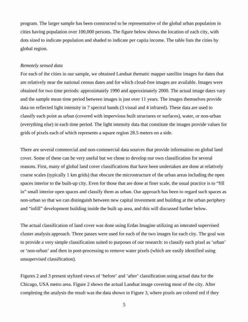
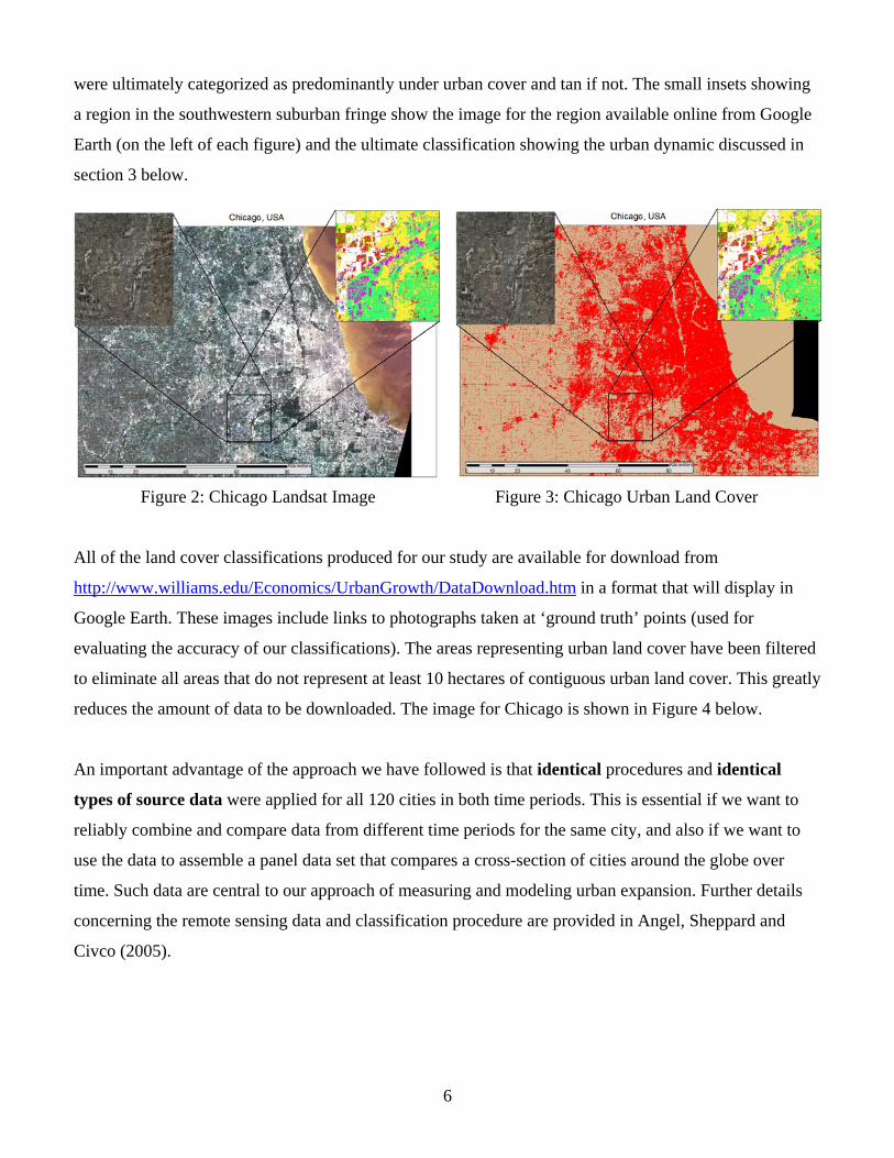
Figures 2 and 3 present stylized views of ‘before’ and ‘after’ classification using actual data for the

Chicago, USA metro area. Figure 2 shows the actual Landsat image covering most of the city. After

completing the analysis the result was the data shown in Figure 3, where pixels are colored red if they

6

were ultimately categorized as predominantly under urban cover and tan if not. The small insets showing

a region in the southwestern suburban fringe show the image for the region available online from Google

Earth (on the left of each figure) and the ultimate classification showing the urban dynamic discussed in

section 3 below.

Figure 2: Chicago Landsat Image Figure 3: Chicago Urban Land Cover

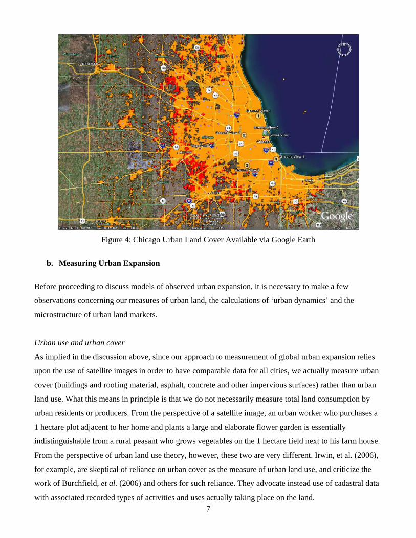
All of the land cover classifications produced for our study are available for download from

http://www.williams.edu/Economics/UrbanGrowth/DataDownload.htm in a format that will display in

Google Earth. These images include links to photographs taken at ‘ground truth’ points (used for

evaluating the accuracy of our classifications). The areas representing urban land cover have been filtered

to eliminate all areas that do not represent at least 10 hectares of contiguous urban land cover. This greatly

reduces the amount of data to be downloaded. The image for Chicago is shown in Figure 4 below.

An important advantage of the approach we have followed is that identical procedures and identical

types of source data were applied for all 120 cities in both time periods. This is essential if we want to

reliably combine and compare data from different time periods for the same city, and also if we want to

use the data to assemble a panel data set that compares a cross-section of cities around the globe over

time. Such data are central to our approach of measuring and modeling urban expansion. Further details

concerning the remote sensing data and classification procedure are provided in Angel, Sheppard and

Civco (2005).

7

Figure 4: Chicago Urban Land Cover Available via Google Earth

b. Measuring Urban Expansion

Before proceeding to discuss models of observed urban expansion, it is necessary to make a few

observations concerning our measures of urban land, the calculations of ‘urban dynamics’ and the

microstructure of urban land markets.

Urban use and urban cover

As implied in the discussion above, since our approach to measurement of global urban expansion relies

upon the use of satellite images in order to have comparable data for all cities, we actually measure urban

cover (buildings and roofing material, asphalt, concrete and other impervious surfaces) rather than urban

land use. What this means in principle is that we do not necessarily measure total land consumption by

urban residents or producers. From the perspective of a satellite image, an urban worker who purchases a

1 hectare plot adjacent to her home and plants a large and elaborate flower garden is essentially

indistinguishable from a rural peasant who grows vegetables on the 1 hectare field next to his farm house.

From the perspective of urban land use theory, however, these two are very different. Irwin, et al. (2006),

for example, are skeptical of reliance on urban cover as the measure of urban land use, and criticize the

work of Burchfield, et al. (2006) and others for such reliance. They advocate instead use of cadastral data

with associated recorded types of activities and uses actually taking place on the land.

8

While the use of cadastral data is no doubt interesting, there are two responses to be made. First is that

many of the most interesting urban areas in the world have very limited cadastral systems and the data

recording actual land uses may either be non-existent or so prone to error that they represent little

improvement over remote sensing data. Second, in practice at the scale of land use in modest to large

urban areas, it seems to make very little difference. Irwin, et al. (2006) compare remotely sensed with

cadastral data in particular areas of the US and while they find the total amounts of land in each category

different, the qualitative nature of changes and even the rates of change of different types of land use are

similar using either measure.

Finally, we note that if one is interested in the ecological, economic or social value of open space then use

of urban land cover data may be preferable. From the perspective of maintaining habitat for a variety of

species or providing positive externalities for which residents are willing to pay, our hypothetical urban

gardener may be as productive, even more so, than the peri-urban farmer. In any event, it should be

acknowledged that the measure of urban expansion and urban land consumption used below is based on

urban cover. We maintain the hypothesis that this measurement is very highly correlated with actual urban

land use in consumption and production. In a sense, the empirical estimates derived below and compared

with theoretical predictions of the comparative static properties of models of urban land use provide a test

of this hypothesis.

Open space and infill development

The simplest theories of urban land markets identify urban land use as clustered around a central business

district of the city, with density of urban land use gradually diminishing as distance from the city

increases. Eventually the value of land in urban use falls to the level where land is more valuable in

agricultural use than in urban use. That distance identifies the maximum extent of urban land use. Up to

this distance, land should all be in urban use and after that distance all land is in agricultural use.

Real cities, of course, are never like this. There are areas of open, unbuilt land within – sometimes deep

within – the urban area. We might regard these as mild departures from the “ideal type” of human

settlement represented by our theory. Alternatively, we might note that these spaces arise for several

reasons: land may be preserved for use as a public good (like a park), land may be owned by a person

with idiosyncratic preferences who prefers the land this way (like our urban gardener discussed above),

9

the land itself may be heterogeneous so that some areas are more difficult to build on due to slope or

drainage, and finally the dynamic structure of the urban economy may generate greater volatility of

structure prices in some areas than in others. Areas with higher volatility present land owners with

increased incentive to hold land vacant since, as observed by Titman (1985) and others, vacant land is

equivalent to an option to buy a building in the future with an exercise price equal to construction costs.

Sheppard (2006) considers this issue explicitly in modeling the microstructure of urban land use, in which

different parts of the city have different levels of coverage by urban surfaces versus open space. The issue

is certainly relevant for understanding why some cities achieve much higher gross population densities

than others and exhibit more compact spatial structure. Measurement of this microstructure at different

points in time allows us to describe more completely the emerging dynamics of urban expansion. In a

simply “von Thunen” style city, urban growth takes a very simple form: an increase in population or

income simply adds another growth ring onto the periphery of the urban area. Again, actual cities exhibit

more complex growth behavior because of the presence of interior unbuilt spaces. Using our classification

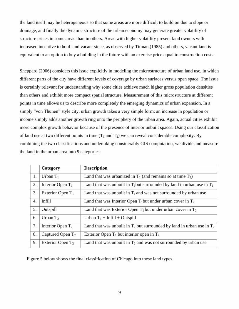
of land use at two different points in time (T1 and T2) we can reveal considerable complexity. By

combining the two classifications and undertaking considerably GIS computation, we divide and measure

the land in the urban area into 9 categories:

Category Description

1. Urban T1 Land that was urbanized in T1 (and remains so at time T2)

2. Interior Open T1 Land that was unbuilt in T1but surrounded by land in urban use in T1

3. Exterior Open T1 Land that was unbuilt in T1 and was not surrounded by urban use

4. Infill Land that was Interior Open T1but under urban cover in T2

5. Outspill Land that was Exterior Open T1 but under urban cover in T2

6. Urban T2 Urban T1 + Infill + Outspill

7. Interior Open T2 Land that was unbuilt in T2 but surrounded by land in urban use in T2

8. Captured Open T2 Exterior Open T1 but interior open in T2

9. Exterior Open T2 Land that was unbuilt in T2 and was not surrounded by urban use

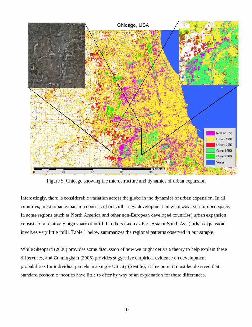
Figure 5 below shows the final classification of Chicago into these land types.

10

Figure 5: Chicago showing the microstructure and dynamics of urban expansion

Interestingly, there is considerable variation across the globe in the dynamics of urban expansion. In all

countries, most urban expansion consists of outspill – new development on what was exterior open space.

In some regions (such as North America and other non-European developed countries) urban expansion

consists of a relatively high share of infill. In others (such as East Asia or South Asia) urban expansion

involves very little infill. Table 1 below summarizes the regional patterns observed in our sample.

While Sheppard (2006) provides some discussion of how we might derive a theory to help explain these

differences, and Cunningham (2006) provides suggestive empirical evidence on development

probabilities for individual parcels in a single US city (Seattle), at this point it must be observed that

standard economic theories have little to offer by way of an explanation for these differences.

11

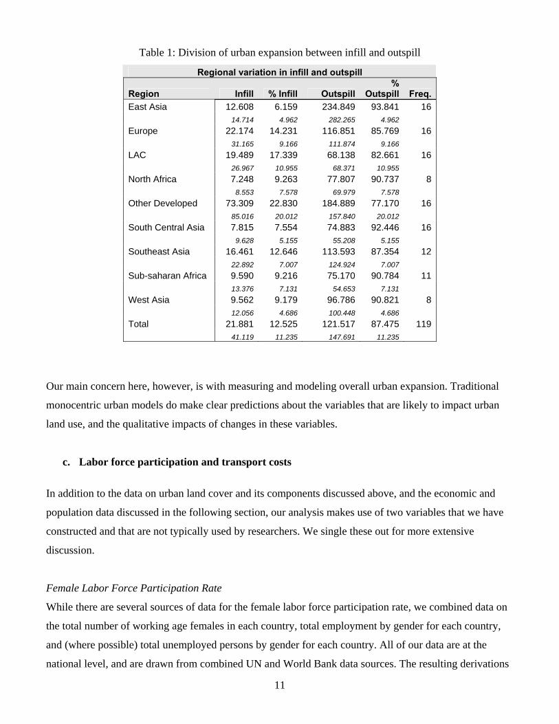
Table 1: Division of urban expansion between infill and outspill

Regional variation in infill and outspill

Region Infill % Infill Outspill%

Outspill Freq. East Asia 12.608 6.159 234.849 93.841 16 14.714 4.962 282.265 4.962 Europe 22.174 14.231 116.851 85.769 16 31.165 9.166 111.874 9.166 LAC 19.489 17.339 68.138 82.661 16 26.967 10.955 68.371 10.955 North Africa 7.248 9.263 77.807 90.737 8 8.553 7.578 69.979 7.578 Other Developed 73.309 22.830 184.889 77.170 16 85.016 20.012 157.840 20.012 South Central Asia 7.815 7.554 74.883 92.446 16 9.628 5.155 55.208 5.155 Southeast Asia 16.461 12.646 113.593 87.354 12 22.892 7.007 124.924 7.007 Sub-saharan Africa 9.590 9.216 75.170 90.784 11 13.376 7.131 54.653 7.131 West Asia 9.562 9.179 96.786 90.821 8 12.056 4.686 100.448 4.686 Total 21.881 12.525 121.517 87.475 119 41.119 11.235 147.691 11.235

Our main concern here, however, is with measuring and modeling overall urban expansion. Traditional

monocentric urban models do make clear predictions about the variables that are likely to impact urban

land use, and the qualitative impacts of changes in these variables.

c. Labor force participation and transport costs

In addition to the data on urban land cover and its components discussed above, and the economic and

population data discussed in the following section, our analysis makes use of two variables that we have

constructed and that are not typically used by researchers. We single these out for more extensive

discussion.

Female Labor Force Participation Rate

While there are several sources of data for the female labor force participation rate, we combined data on

the total number of working age females in each country, total employment by gender for each country,

and (where possible) total unemployed persons by gender for each country. All of our data are at the

national level, and are drawn from combined UN and World Bank data sources. The resulting derivations

12

compare reasonably well with published results for the female labor force participation rate in countries

(like the US) where the participation rate is routinely calculated and reported.

We calculated participation rates for each time period for the year in which the satellite image used to

measure urban land cover was collected. Most cities experienced an increase in the FLFPR during the

time period between the images. As shown in Table 2 below, the average increase is about .09. There is

considerable variation, however, across the sample. There are 15 cities that experienced decreases in the

FLFPR, with the largest decrease being a decline of -0.28. Eight of these cities were in countries that also

experienced declines in real incomes. There were 7 cities in 4 countries (Egypt, Turkey, Hungary and

Poland) that appear to have experienced declines in the FLFPR while also experiencing increases

(although modest) in real incomes.

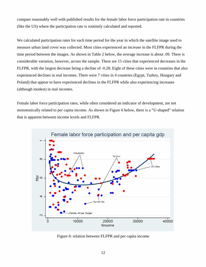
Female labor force participation rates, while often considered an indicator of development, are not

monotonically related to per capita income. As shown in Figure 6 below, there is a “U-shaped” relation

that is apparent between income levels and FLFPR.

Figure 6: relation between FLFPR and per capita income

13

In the figure, the blue dots indicate the position of a city at the time of the first image (approximately

1990) and the red dots correspond to the time of the second image (approximately 2000).

Time cost of travel

We make use of two variables to capture the time cost of travel. The first is the real cost of motor fuel at

the pump, taken from World Bank data sources. Naturally, the fuel costs are only a small part of the total

costs of travel, with time costs generally being more significant in household decision making. In

empirical models that focus on a single city, it is generally safe to rely on a single measure because the

price of motor fuel is roughly equal throughout the urban area, and the fuel costs are highly correlated

with the time costs of travel.

When modeling urban form across a global cross-section of cities, however, this comfortable relationship

breaks down. Road capacity varies greatly between cities, affecting the average speed of travel. In

addition, local wage rates vary so that the economic sacrifice associated with commuting varies. To

address this problem, we have relied on data collected by our field researchers in each of the 120 cities in

our sample.

Each field researcher was asked to travel by car to each of 4 or 5 different points within the urban area.

They recorded the time elapsed between each point, and the total number of kilometers traveled. They

also collected (using a handheld GPS device) the exact coordinates of the location for each stop. An

example, Figure 7 below shows the urban land cover for Budapest, Hungary. The five locations labeled

“Ground View” are the five stops on the journey around the city taken by our field researcher.

This information was used to calculate an average speed of travel during the journey. The speed data were

then combined with information collected on local incomes to produce an estimate of the time cost per

kilometer of travel. As shown in Table 2 below, this averages 0.25 $ppp per kilometer of travel, but varies

from a minimum of .01 to a maximum of $1.73. These data provide a novel opportunity to examine the

impact of changing the time costs of travel on urban form, and permit a more careful filtering of this cost

to assist in isolating the separate impact of female labor force participation.

14

Figure 7: Budapest, Hungary – showing ‘Ground View’ locations

d. Other economic variables

The urban land cover data described above are matched with population data for jurisdictional boundaries

in each area, obtained from the Center for International Earth Science Information Network’s Global

Rural-Urban Mapping Project. Using growth rates observed for each jurisdiction during 1980 through

2000 we interpolate to obtain population estimates for the dates of each image. There are many cases

where the Landsat images did not provide complete coverage of the jurisdictional boundaries for which

population data were available. In these cases we sometimes purchased additional Landsat images, but in

other cases made use of an interpolation procedure using our land cover classification and distance from

the urban center to apportion the jurisdiction population between portions covered by our remote sensing

images and the portions not covered. In general the data include not only the jurisdictions covering the

central city and largest contiguous regions of classified urban land cover, but extend to peripheral

jurisdictions until the mean size of contiguous urban cluster falls below 25 hectares. This provides

coverage that approximates a “metro area” definition for all cities even though for most of the cities we

15

lack the data on labor markets and commuting patterns generally required for formal definition of such

areas.

We also interpolate national per capita GDP to the date of the satellite image to provide an estimate of

income levels in each city matched to the remote sensing data. Data on biome type, availability of shallow

groundwater aquifer, air transport links, and the value of agricultural land (approximated by agricultural

output per hectare) were obtained from World Development Indicators or from sources described more

fully in Angel, Sheppard and Civco (2005)

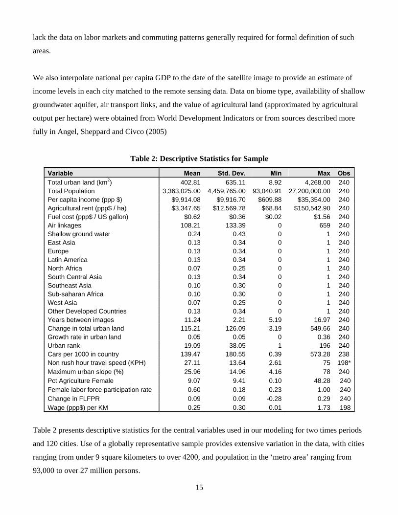
Table 2: Descriptive Statistics for Sample

Variable Mean Std. Dev. Min Max ObsTotal urban land (km2) 402.81 635.11 8.92 4,268.00 240 Total Population 3,363,025.00 4,459,765.00 93,040.91 27,200,000.00 240 Per capita income (ppp $) $9,914.08 $9,916.70 $609.88 $35,354.00 240 Agricultural rent (ppp$ / ha) $3,347.65 $12,569.78 $68.84 $150,542.90 240 Fuel cost (ppp$ / US gallon) $0.62 $0.36 $0.02 $1.56 240 Air linkages 108.21 133.39 0 659 240 Shallow ground water 0.24 0.43 0 1 240 East Asia 0.13 0.34 0 1 240 Europe 0.13 0.34 0 1 240 Latin America 0.13 0.34 0 1 240 North Africa 0.07 0.25 0 1 240 South Central Asia 0.13 0.34 0 1 240 Southeast Asia 0.10 0.30 0 1 240 Sub-saharan Africa 0.10 0.30 0 1 240 West Asia 0.07 0.25 0 1 240 Other Developed Countries 0.13 0.34 0 1 240 Years between images 11.24 2.21 5.19 16.97 240 Change in total urban land 115.21 126.09 3.19 549.66 240 Growth rate in urban land 0.05 0.05 0 0.36 240 Urban rank 19.09 38.05 1 196 240 Cars per 1000 in country 139.47 180.55 0.39 573.28 238 Non rush hour travel speed (KPH) 27.11 13.64 2.61 75 198*Maximum urban slope (%) 25.96 14.96 4.16 78 240 Pct Agriculture Female 9.07 9.41 0.10 48.28 240Female labor force participation rate 0.60 0.18 0.23 1.00 240Change in FLFPR 0.09 0.09 -0.28 0.29 240Wage (ppp$) per KM 0.25 0.30 0.01 1.73 198

Table 2 presents descriptive statistics for the central variables used in our modeling for two times periods

and 120 cities. Use of a globally representative sample provides extensive variation in the data, with cities

ranging from under 9 square kilometers to over 4200, and population in the ‘metro area’ ranging from

93,000 to over 27 million persons.

16

In addition to the variables used in the models of urban expansion presented below, Table 2 provides

information on additional variables that are likely to be of interest. While the sample includes many

primate cities (of rank 1 in the national urban system) it includes cities down to rank 196 as well. The rate

of automobile ownership varies across the sample even more than per capita income, although in general

it is income rather than automobile ownership that turns out to be the most important factor influencing

total urban land cover. In part this may be because increased automobile ownership does not necessarily

imply reduced transportation costs, since congestion can slow travel considerably below the maximum

speed of the vehicle. The average non-rush hour travels speeds are seen to vary widely. These have been

collected by our field researchers.

IV. Analysis

Our data permit two types of test of the prediction that increasing FLFPR will be associated with reduced

urban expansion. One is to estimate the impact based on the change, in each city, of total urban land use

as a function of the change in population, change in income, change in the female labor force participation

rate, and changes in agricultural land values, global linkages, fuel costs in each city. There are two

difficulties with this approach. First is that it reduces our sample size from to 118 cities (the number for

which we have all of these variables at both time periods. The second problem is that while we might be

comfortable using average travel speeds measured by our field researchers as applying to both the time

period of the first and of the second images, if we take the first difference of these we will have no

variation in the sample to determine an impact of the time cost of travel.

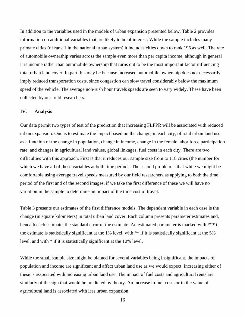
Table 3 presents our estimates of the first difference models. The dependent variable in each case is the

change (in square kilometers) in total urban land cover. Each column presents parameter estimates and,

beneath each estimate, the standard error of the estimate. An estimated parameter is marked with *** if

the estimate is statistically significant at the 1% level, with ** if it is statistically significant at the 5%

level, and with * if it is statistically significant at the 10% level.

While the small sample size might be blamed for several variables being insignificant, the impacts of

population and income are significant and affect urban land use as we would expect: increasing either of

these is associated with increasing urban land use. The impact of fuel costs and agricultural rents are

similarly of the sign that would be predicted by theory. An increase in fuel costs or in the value of

agricultural land is associated with less urban expansion.

17

Most interestingly from the perspective of the central question of this paper, an increase in the female

labor force participation rate is associated with a reduced level of urban expansion after adjusting for the

other factors in the model. The estimate imprecise and not statistically significant in models 1 and 2, but

does (barely) reach significance at the 10 percent level in model 3. Overall, it would seem that our first-

difference models offer confirmation, if somewhat weak, of the expected impact.

Table 3: First-difference models of urban expansion Variable Model 1 Model 2 Model 3 ∆ Population 0.0001*** 0.0001*** 0.0001*** 0.0000 0.0000 0.0000 ∆ Income 0.0074*** 0.0074*** 0.0074*** 0.0020 0.0020 0.0020 ∆ Air linkages -0.0026 0.2260 ∆ Agric Rent -0.0118 -0.0118 -0.0118 0.0090 0.0080 0.0080 ∆ FLFPR -171.9459 -171.9566 -172.3025* 107.8490 107.3530 106.5550 ∆ Fuel Cost -2.6923 -2.698 -2.0949 52.4800 52.2390 50.0010 T1 Agric Rent -0.0057** -0.0057** -0.0057** 0.0030 0.0030 0.0020 T1 Fuel Cost 1.5449 1.5471 36.9910 36.8220

F 11.19 12.91 15.2 Adj R2 0.4107 0.4161 0.4213 Root MSE 97.779 97.333 96.894

Our next set of models incorporates a much richer set of variables, taking each city in each time period as

an “observation” and correcting for clusters and variables fixed within cities by including fixed effects

variables for all cities.

In these models endogeneity is of particular concern, since income producing activities and population

might be differentially attracted to large (or expansive) cities. Each model is therefore estimated using an

instrumental variables approach. The instruments used for the estimation are the same as were used in

Blomberg and Sheppard (2007), and make use of local environmental conditions and climate. The

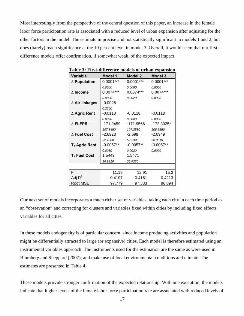
estimates are presented in Table 4.

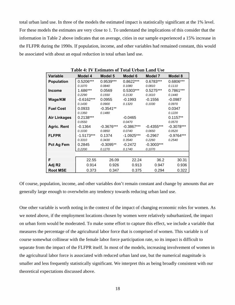
These models provide stronger confirmation of the expected relationship. With one exception, the models

indicate that higher levels of the female labor force participation rate are associated with reduced levels of

18

total urban land use. In three of the models the estimated impact is statistically significant at the 1% level.

For these models the estimates are very close to 1. To understand the implications of this consider that the

information in Table 2 above indicates that on average, cities in our sample experienced a 15% increase in

the FLFPR during the 1990s. If population, income, and other variables had remained constant, this would

be associated with about an equal reduction in total urban land use.

Table 4: IV Estimates of Total Urban Land Use Variable Model 4 Model 5 Model 6 Model 7 Model 8 Population 0.5206*** 0.9539*** 0.8622*** 0.6783*** 0.6806*** 0.1070 0.0840 0.1080 0.0810 0.1110 Income 1.686*** 0.0569 0.5303*** 0.5275*** 0.7861*** 0.2290 0.1550 0.2130 0.1610 0.1440 Wage/KM -0.6162*** 0.0955 -0.1993 -0.1556 -0.0987 0.1430 0.0900 0.1320 0.1030 0.0970 Fuel Cost 0.0933 -0.3541** 0.0347 0.1350 0.1480 0.1220 Air Linkages 0.2138*** -0.0465 0.1157** 0.0550 0.0470 0.0570 Agric. Rent -0.1364 -0.3676*** -0.3867*** -0.4355*** -0.3078*** 0.1030 0.0850 0.0740 0.0650 0.0520 FLFPR -1.5173*** 0.1374 -1.0925*** -0.2967 -0.9764*** 0.3310 0.3430 0.3540 0.2260 0.2540 Pct Ag Fem 0.2845 -0.3095** -0.2472 -0.3003*** 0.2200 0.1270 0.1740 0.1070

F 22.55 26.09 22.24 36.2 30.31 Adj R2 0.914 0.926 0.913 0.947 0.936 Root MSE 0.373 0.347 0.375 0.294 0.322

Of course, population, income, and other variables don’t remain constant and change by amounts that are

generally large enough to overwhelm any tendency towards reducing urban land use.

One other variable is worth noting in the context of the impact of changing economic roles for women. As

we noted above, if the employment locations chosen by women were relatively suburbanized, the impact

on urban form would be moderated. To make some effort to capture this effect, we include a variable that

measures the percentage of the agricultural labor force that is comprised of women. This variable is of

course somewhat collinear with the female labor force participation rate, so its impact is difficult to

separate from the impact of the FLFPR itself. In most of the models, increasing involvement of women in

the agricultural labor force is associated with reduced urban land use, but the numerical magnitude is

smaller and less frequently statistically significant. We interpret this as being broadly consistent with our

theoretical expectations discussed above.

19

V. Conclusions We have collected and made use of a unique global data set on urban land use and its driving forces.

Using these data, we ask a simple question: what is the impact, holding other factors constant, of

increasing the female labor force participation rate? Theoretically, we expect increasing FLFPR to be

associated with more compact cities.

We consider both simple first difference models of urban land use and cross-section models estimated

using instrumental variable techniques. In general we find support for the theoretical predictions. An

increase in the FLFPR appears to be associated, ceteris paribus, with reduced urban land use.

20

VI. Bibliography Angel, S., Sheppard, S. and Civco, D. (2005), The Dynamics of Global Urban Expansion, Washington:

The World Bank. Available online at www.williams.edu/Economics/UrbanGrowth/WorkingPapers.htm or http://www.citiesalliance.org/publications/homepage-features/feb-06/urban-expansion.html

Breheny, Michael, (1995), The compact city and transport energy consumption, Transactions of the Institute of British Geographers, 20, 81-101.

Brueckner, J., (1987), The Structure of Urban Equilibria, Chapter 20 in Handbook of Regional and Urban

Economics, E. Mills, ed., New York: Elsevier. Brueckner, J. and Largey, A., (2007), Social Interaction and Urban Sprawl, unpublished working paper. Burchfeld, N., Overman, H., Puga, D. and Turner, M. (2006), Sprawl: A View from Space, Quarterly

Journal of Economics, 121, 587-633. Cunningham, C. (2006), House price uncertainty, timing of development, and vacant land prices:

Evidence for real options in Seattle, Journal of Urban Economics, 59, 1-31. Irwin, E. and Bockstael, N., (2006) Measuring and Modeling Urban Sprawl: Data, Scale and Spatial

Dependencies, unpublished working paper.

Newman P and Kenworthy J., (1989) Gasoline consumption and cities: a comparison of UK cities with a global survey, Journal of the American Planning Association, 55, 24-37.

Sheppard, Stephen, (2006), Infill versus Outspill: the microstructure of urban expansion, Williams

College Working Papers in Economics. Power, Anne, (2001), Social Exclusion and Urban Sprawl: Is the Rescue of Cities Possible?, Regional

Studies, 35:8, 731-742. Titman, Sheridan, (1985) Urban Land Prices Under Uncertainty, American Economic Review, 75, 505-

514. Wu, Weiping and Yusuf, Shahid, (2004), Shanghai: remaking China’s future global city, in Gugler, J. (ed)

World Cities Beyond the West, Cambridge: Cambridge University Press.