1

Gene Selection for Cancer Classification usingSupport Vector Machines

Isabelle Guyon+, Jason Weston+, Stephen Barnhill, M.D.+and Vladimir Vapnik*

+Barnhill Bioinformatics, Savannah, Georgia, USA* AT&T Labs, Red Bank, New Jersey, USA

Address correspondence to:Isabelle Guyon, 955 Creston Road, Berkeley, CA 94708. Tel: (510) 524 6211.Email: isabelle@barnhilltechnologies.comSubmitted to Machine Learning.

SummaryDNA micro-arrays now permit scientists to screen thousands of genessimultaneously and determine whether those genes are active, hyperactive orsilent in normal or cancerous tissue. Because these new micro-array devicesgenerate bewildering amounts of raw data, new analytical methods must bedeveloped to sort out whether cancer tissues have distinctive signatures of geneexpression over normal tissues or other types of cancer tissues.

In this paper, we address the problem of selection of a small subset of genesfrom broad patterns of gene expression data, recorded on DNA micro-arrays.Using available training examples from cancer and normal patients, we build aclassifier suitable for genetic diagnosis, as well as drug discovery. Previousattempts to address this problem select genes with correlation techniques. Wepropose a new method of gene selection utilizing Support Vector Machinemethods based on Recursive Feature Elimination (RFE). We demonstrateexperimentally that the genes selected by our techniques yield betterclassification performance and are biologically relevant to cancer.

In contrast with the baseline method, our method eliminates gene redundancyautomatically and yields better and more compact gene subsets. In patients withleukemia our method discovered 2 genes that yield zero leave-one-out error,while 64 genes are necessary for the baseline method to get the best result (oneleave-one-out error). In the colon cancer database, using only 4 genes ourmethod is 98% accurate, while the baseline method is only 86% accurate.

Keywords

Diagnosis, diagnostic tests, drug discovery, RNA expression, genomics, geneselection, DNA micro-array, proteomics, cancer classification, feature selection,Support Vector Machines, Recursive Feature Elimination.

2

I. IntroductionThe advent of DNA micro-array technology has brought to data analysts broadpatterns of gene expression simultaneously recorded in a single experiment(Fodor, 1997). In the past few months, several data sets have become publiclyavailable on the Internet. These data sets present multiple challenges, includinga large number of gene expression values per experiment (several thousands totens of thousands), and a relatively small number of experiments (a few dozen).

The data can be analyzed from many different viewpoints. The literature alreadyabounds in studies of gene clusters discovered by unsupervised learningtechniques (see e.g. (Eisen, 1998) (Perou, 1999) (Alon, 1999), and (Alizadeh,2000)). Clustering is often done along the other dimension of the data. Forexample, each experiment may correspond to one patient carrying or notcarrying a specific disease (see e.g. (Golub, 1999)). In this case, clusteringusually groups patients with similar clinical records. Recently, supervisedlearning has also been applied, to the classification of proteins (Brown, 2000)and to cancer classification (Golub, 1999).

This last paper on leukemia classification presents a feasibility study of diagnosisbased solely on gene expression monitoring. In the present paper, we go furtherin this direction and demonstrate that, by applying state-of-the-art classificationalgorithms (Support Vector Machines (Boser, 1992), (Vapnik, 1998)), a smallsubset of highly discriminant genes can be extracted to build very reliable cancerclassifiers. We make connections with related approaches that were developedindependently, which either combine ((Furey, 2000), (Pavlidis, 2000)) or integrate((Mukherjee,1999), (Chapelle, 2000), (Weston, 2000)) feature selection withSVMs.

The identification of discriminant genes is of fundamental and practical interest.Research in Biology and Medicine may benefit from the examination of the topranking genes to confirm recent discoveries in cancer research or suggest newavenues to be explored. Medical diagnostic tests that measure the abundance ofa given protein in serum may be derived from a small subset of discriminantgenes.

This application also illustrates new aspects of the applicability of Support VectorMachines (SVMs) in knowledge discovery and data mining. SVMs were alreadyknown as a tool that discovers informative patterns (Guyon, 1996). The presentapplication demonstrates that SVMs are also very effective for discoveringinformative features or attributes (such as critically important genes). In acomparison with several other gene selection methods on Colon cancer data(Alon, 1999) we demonstrate that SVMs have both quantitative and qualitativeadvantages. Our techniques outperform other methods in classificationperformance for small gene subsets while selecting genes that have plausiblerelevance to cancer diagnosis.

3

After formally stating the problem and reviewing prior work (Section II), wepresent in Section III a new method of gene selection using SVMs. Before turningto the experimental section (Section V), we describe the data sets under studyand provide the basis of our experimental method (Section IV). Particular care isgiven to evaluate the statistical significance of the results for small sample sizes.In the discussion section (Section VI), we review computational complexityissues, contrast qualitatively our feature selection method with others, andpropose possible extensions of the algorithm.

II. Problem description and prior work

II.1. Classification problemsIn this paper we address classification problems where the input is a vector thatwe call a “pattern” of n components which we call “features”. We call F the n-dimensional feature space. In the case of the problem at hand, the features aregene expression coefficients and patterns correspond to patients. We limitourselves to two-class classification problems. We identify the two classes with

the symbols (+) and (-). A training set of a number of patterns {x1, x2, … xk, …xl}

with known class labels {y1, y2, … yk, … yl}, yk∈{-1,+1}, is given. The trainingpatterns are used to build a decision function (or discriminant function) D(x), thatis a scalar function of an input pattern x. New patterns are classified according tothe sign of the decision function:

D(x) > 0 ⇒ x ∈ class (+)D(x) < 0 ⇒ x ∈ class (-)D(x) = 0, decision boundary.

Decision functions that are simple weighted sums of the training patterns plus abias are called linear discriminant functions (see e.g. (Duda, 73)). In ournotations:

D(x) = w.x+b, (1)where w is the weight vector and b is a bias value.A data set is said to be “linearly separable” if a linear discriminant function canseparate it without error.

II.2. Space dimensionality reduction and feature selectionA known problem in classification specifically, and machine learning in general, isto find ways to reduce the dimensionality n of the feature space F to overcomethe risk of “overfitting”. Data overfitting arises when the number n of features islarge (in our case thousands of genes) and the number l of training patterns iscomparatively small (in our case a few dozen patients). In such a situation, onecan easily find a decision function that separates the training data (even a lineardecision function) but will perform poorly on test data. Training techniques thatuse regularization (see e.g. (Vapnik, 1998)) avoid overfitting of the data to someextent without requiring space dimensionality reduction. Such is the case, forinstance, of Support Vector Machines (SVMs) ((Boser, 1992), (Vapnik, 1998),

4

(Cristianini, 1999)). Yet, as we shall see from experimental results (Section V),even SVMs benefit from space dimensionality reduction.

Projecting on the first few principal directions of the data is a method commonlyused to reduce feature space dimensionality (see, e.g. (Duda, 73)). With such amethod, new features are obtained that are linear combinations of the originalfeatures. One disadvantage of projection methods is that none of the originalinput features can be discarded. In this paper we investigate pruning techniquesthat eliminate some of the original input features and retain a minimum subset offeatures that yield best classification performance. Pruning techniques lendthemselves to the applications that we are interested in. To build diagnostic tests,it is of practical importance to be able to select a small subset of genes. Thereasons include cost effectiveness and ease of verification of the relevance ofselected genes.

The problem of feature selection is well known in machine learning. For a reviewof feature selection, see e.g. (Kohavi, 1997). Given a particular classificationtechnique, it is conceivable to select the best subset of features satisfying a given“model selection” criterion by exhaustive enumeration of all subsets of features.For a review of model selection, see e.g. (Kearns, 1997). Exhaustiveenumeration is impractical for large numbers of features (in our case thousandsof genes) because of the combinatorial explosion of the number of subsets. Inthe discussion section (Section VI), we shall go back to this method that can beused in combination with another method that first reduces the number offeatures to a manageable size.

Performing feature selection in large dimensional input spaces therefore involvesgreedy algorithms. Among various possible methods feature-ranking techniquesare particularly attractive. A fixed number of top ranked features may be selectedfor further analysis or to design a classifier. Alternatively, a threshold can be seton the ranking criterion. Only the features whose criterion exceeds the thresholdare retained. In the spirit of Structural Risk Minimization (see e.g. Vapnik, 1998and Guyon, 1992) it is possible to use the ranking to define nested subsets offeatures F1 ⊂ F2 ⊂ … ⊂ F, and select an optimum subset of features with amodel selection criterion by varying a single parameter: the number of features.In the following, we compare several feature-ranking algorithms.

II.3. Feature ranking with correlation coefficientsIn the test problems under study, it is not possible to achieve an errorlessseparation with a single gene. Better results are obtained when increasing thenumber of genes. Classical gene selection methods select the genes thatindividually classify best the training data. These methods include correlationmethods and expression ratio methods. They eliminate genes that are uselessfor discrimination (noise), but they do not yield compact gene sets becausegenes are redundant. Moreover, complementary genes that individually do notseparate well the data are missed.

5

Evaluating how well an individual feature contributes to the separation (e.g.cancer vs. normal) can produce a simple feature (gene) ranking. Variouscorrelation coefficients are used as ranking criteria. The coefficient used in(Golub , 1999) is defined as:

wi = (µi(+) – µ i(-)) / (σ i(+)+ σi(-)) (2)where µ i and σi are the mean and standard deviation of the gene expressionvalues of gene i for all the patients of class (+) or class (-), i=1,…n. Large positivewi values indicate strong correlation with class (+) whereas large negative wivalues indicate strong correlation with class (-). The original method of (Golub,1999) is to select an equal number of genes with positive and with negativecorrelation coefficient. Others (Furey, 2000) have been using the absolute valueof wi as ranking criterion. Recently, in (Pavlidis, 2000), the authors have beenusing a related coefficient (µi(+) – µi(-))2 / (σi(+)2 + σi(-)2), which is similar toFisher’s discriminant criterion (Duda, 1973).What characterizes feature ranking with correlation methods is the implicitorthogonality assumptions that are made. Each coefficient wi is computed withinformation about a single feature (gene) and does not take into account mutualinformation between features. In the next section, we explain in more detailswhat such orthogonality assumptions mean.

II. 4. Ranking criterion and classificationOne possible use of feature ranking is the design of a class predictor (orclassifier) based on a pre-selected subset of features. Each feature that iscorrelated (or anti-correlated) with the separation of interest is by itself such aclass predictor, albeit an imperfect one. This suggests a simple method ofclassification based on weighted voting: the features vote proportionally to theircorrelation coefficient. Such is the method being used in (Golub, 1999). Theweighted voting scheme yields a particular linear discriminant classifier:

D(x) = w.(x-µ) (3)where w is defined in Equation (2) and µ = (µ(+) + µ(-))/2.It is interesting to relate this classifier to Fisher’s linear discriminant. Such aclassifier is also of the form of Equation (3), with

w = S-1 (µ(+) – µ(-)), where S is the (n, n) within class scatter matrix defined as

S = ∑+∈ )(Xx

(x-µ(+))(x-µ(+))T + ∑−∈ )(Xx

(x-µ(-))(x-µ(-))T

And where µ is the mean vector over all training patterns. We denote by X(+) andX(-) the training sets of class (+) and (-). This particular form of Fisher’s lineardiscriminant implies that S is invertible. This is not the case if the number offeatures n is larger than the number of examples l since then the rank of S is atmost l. The classifier of (Golub, 1999) and Fisher’s classifier are particularlysimilar in this formulation if the scatter matrix is approximated by its diagonalelements. This approximation is exact when the vectors formed by the values ofone feature across all training patterns are orthogonal, after subtracting the classmean. It retains some validity if the features are uncorrelated, that is if the

6

expected value of the product of two different feature is zero, after removing theclass mean. Approximating S by its diagonal elements is one way of regularizingit (making it invertible). But, in practice, features are usually correlated andtherefore the diagonal approximation is not valid.

We have just established that the feature ranking coefficients can be used asclassifier weights. Reciprocally, the weights multiplying the inputs of a givenclassifier can be used as feature ranking coefficients. The inputs that areweighted by the largest value influence most the classification decision.Therefore, if the classifier performs well, those inputs with the largest weightscorrespond to the most informative features. This scheme generalizes theprevious one. In particular, there exist many algorithms to train lineardiscriminant functions that may provide a better feature ranking than correlationcoefficients. These algorithms include Fisher’s linear discriminant, justmentioned, and SVMs that are the subject of this paper. Both methods areknown in statistics as “multivariate” classifiers, which means that they areoptimized during training to handle multiple variables (or features)simultaneously. The method of (Golub, 1999), in contrast, is a combination ofmultiple “univariate” classifiers.

II.5. Feature ranking by sensitivity analysisIn this Section, we show that ranking features with the magnitude of the weightsof a linear discriminant classifier is a principled method. Several authors havesuggested to use the change in objective function when one feature is removedas a ranking criterion (Kohavi, 1997). For classification problems, the idealobjective function is the expected value of the error, that is the error ratecomputed on an infinite number of examples. For the purpose of training, thisideal objective is replaced by a cost function J computed on training examplesonly. Such a cost function is usually a bound or an approximation of the idealobjective, chosen for convenience and efficiency reasons. Hence the idea tocompute the change in cost function DJ(i) caused by removing a given feature or,equivalently, by bringing its weight to zero. The OBD algorithm (LeCun, 1990)approximates DJ(i) by expanding J in Taylor series to second order. At theoptimum of J, the first order term can be neglected, yielding:

DJ(i) = (1/2) 2

2

iwJ

∂∂

(Dwi)2 (4)

The change in weight Dwi = wi corresponds to removing feature i. The authors ofthe OBD algorithm advocate using DJ(i) instead of the magnitude of the weightsas a weight pruning criterion. For linear discriminant functions whose costfunction J is a quadratic function of wi these two criteria are equivalent. This isthe case for example of the mean-squared-error classifier (Duda, 1973) with costfunction J= ∑

∈Xx

||w.x-y||2 and linear SVMs ((Boser, 1992), (Vapnik, 1998),

(Cristianini, 1999)), which minimize J=(1/2)||w ||2, under constrains. This justifiesthe use of (wi)2 as a feature ranking criterion.

7

II.6. Recursive Feature eliminationA good feature ranking criterion is not necessarily a good feature subset rankingcriterion. The criteria DJ(i) or (wi)2 estimate the effect of removing one feature ata time on the objective function. They become very sub-optimal when it comes toremoving several features at a time, which is necessary to obtain a small featuresubset. This problem can be overcome by using the following iterative procedurethat we call Recursive Feature Elimination:1) Train the classifier (optimize the weights wi with respect to J).2) Compute the ranking criterion for all features (DJ(i) or (wi)2).3) Remove the feature with smallest ranking criterion.

This iterative procedure is an instance of backward feature elimination ((Kohavi,2000) and references therein). For computational reasons, it may be moreefficient to remove several features at a time, at the expense of possibleclassification performance degradation. In such a case, the method produces afeature subset ranking, as opposed to a feature ranking. Feature subsets arenested F1 ⊂ F2 ⊂ … ⊂ F.

If features are removed one at a time, there is also a corresponding featureranking. However, the features that are top ranked (eliminated last) are notnecessarily the ones that are individually most relevant. Only taken together thefeatures of a subset F m are optimal in some sense.

In should be noted that RFE has no effect on correlation methods since theranking criterion is computed with information about a single feature.

III. Feature ranking with Support Vector Machines

III.1. Support Vector Machines (SVM)To test the idea of using the weights of a classifier to produce a feature ranking,we used a state-of-the-art classification technique: Support Vector Machines(SVMs) (Boser, 1992; Vapnik, 1998). SVMs have recently been intensivelystudied and benchmarked against a variety of techniques (see for instance,(Guyon, 1999)). They are presently one of the best-known classificationtechniques with computational advantages over their contenders (Cristianini,1999).

Although SVMs handle non-linear decision boundaries of arbitrary complexity, welimit ourselves, in this paper, to linear SVMs because of the nature of the datasets under investigation. Linear SVMs are particular linear discriminant classifiers(see Equation (1)). An extension of the algorithm to the non-linear case can befound in the discussion section (Section VI). If the training data set is linearlyseparable, a linear SVM is a maximum margin classifier. The decision boundary(a straight line in the case of a two-dimensional separation) is positioned to leavethe largest possible margin on either side. A particularity of SVMs is that theweights wi of the decision function D(x) are a function only of a small subset of

8

the training examples, called “support vectors”. Those are the examples that areclosest to the decision boundary and lie on the margin. The existence of suchsupport vectors is at the origin of the computational properties of SVM and theircompetitive classification performance. While SVMs base their decision functionon the support vectors that are the borderline cases, other methods such as themethod used by Golub et al (Golub, 1999) base their decision function on theaverage case. As we shall see in the discussion section (Section VI), this hasalso consequences on the feature selection process.

In this paper, we use one of the variants of the soft-margin algorithm described in(Cortes, 1995). Training consists in executing the following quadratic program:

Algorithm SVM-train:

Inputs:Training examples {x1, x2, … xk, …xl} and class labels {y1, y2, … yk, … yl}.Minimize over αk:J = (1/2) ∑

hk

yh yk αh αk (xh.xk + λ δhk) - ∑k

αk (5)

subject to:0 ≤ αk ≤ C and ∑

k

αk yk =0

Outputs: Parameters αk.

The summations run over all training patterns xk that are n dimensional featurevectors, xh.xk denotes the scalar product, yk encodes the class label as a binaryvalue +1 or –1, δhk is the Kronecker symbol (δhk=1 if h=k and 0 otherwise), and λand C are positive constants (soft margin parameters). The soft marginparameters ensure convergence even when the problem is non-linearlyseparable or poorly conditioned. In such cases, some of the support vectors maynot lie on the margin. Most authors use either λ or C. We use a small value of λ(of the order of 10-14) to ensure numerical stability. For the problems under study,the solution is rather insensitive to the value of C because the training data setsare linearly separable down to just a few features. A value of C=100 is adequate.

The resulting decision function of an input vector x is:D(x) = w.x + bwithw = ∑

k

αk yk xk and b=⟨yk-w.xk⟩

The weight vector w is a linear combination of training patterns. Most weights αk

are zero. The training patterns with non-zero weights are support vectors. Thosewith weight satisfying the strict inequality 0<αk<C are marginal support vectors.The bias value b is an average over marginal support vectors.Many resources on support vector machines, including computerimplementations can be found at: http://www.kernel-machines.org.

9

III.2. SVM Recursive Feature Elimination (SVM RFE)SVM RFE is an application of RFE using the weight magnitude as rankingcriterion.We present below an outline of the algorithm in the linear case, using SVM-trainin Equation (5). An extension to the non-linear case is proposed in the discussionsection (Section VI).

Algorithm SVM-RFE:Inputs:Training examples

X0 = [x1, x2, … xk, …xl]T

Class labels

y = [y1, y2, … yk, … yl]T

Initialize:Subset of surviving features

s = [1, 2, … n]Feature ranked list

r = [ ]Repeat until s = [ ]Restrict training examples to good feature indices

X = X0(:, s)Train the classifier

α = SVM-train(X, y)Compute the weight vector of dimension length(s)

w = ∑k

αk yk xk

Compute the ranking criteriaci = (wi)2, for all i

Find the feature with smallest ranking criterionf = argmin(c)

Update feature ranked listr = [s(f), r]

Eliminate the feature with smallest ranking criterions = s(1:f-1, f+1:length(s))

Output:Feature ranked list r.

As mentioned before the algorithm can be generalized to remove more than onefeature per step for speed reasons.

10

IV. Material and experimental method

IV.1. Description of the data setsWe present results on two data sets both of which consist of a matrix of geneexpression vectors obtained from DNA micro-arrays (Fodor, 1997) for a numberof patients. The first set was obtained from cancer patients with two differenttypes of leukemia. The second set was obtained from cancerous or normal colontissues. Both data sets proved to be relatively easy to separate. Afterpreprocessing, it is possible to find a weighted sum of a set of only a few genesthat separates without error the entire data set (the data set is linearlyseparable). Although the separation of the data is easy, the problems presentseveral features of difficulty, including small sample sizes and data differentlydistributed between training and test set (in the case of leukemia).

One particularly challenging problem in the case of the colon cancer data is that“tumor” samples and “normal” samples differ in cell composition. Tumors aregenerally rich in epithelial (skin) cells whereas normal tissues contain a variety ofcells, including a large fraction of smooth muscle cells. Therefore, the samplescan easily be split on the basis of cell composition, which is not informative fortracking cancer-related genes.

1) Differentiation of two types of LeukemiaIn (Golub, 1999), the authors present methods for analyzing gene expressiondata obtained from DNA micro-arrays in order to classify types of cancer. Theirmethod is illustrated on leukemia data that is available on-line.

The problem is to distinguish between two variants of leukemia (ALL and AML).The data is split into two subsets: A training set, used to select genes and adjustthe weights of the classifiers, and an independent test set used to estimate theperformance of the system obtained. Their training set consists of 38 samples(27 ALL and 11 AML) from bone marrow specimens. Their test set has 34samples (20 ALL and 14 AML), prepared under different experimental conditionsand including 24 bone marrow and 10 blood sample specimens. All sampleshave 7129 features, corresponding to some normalized gene expression valueextracted from the micro-array image. We retained the exact same experimentalconditions for ease of comparison with their method.

In our preliminary experiments, some of the large deviations between leave-one-out error and test error could not be explained by the small sample size alone.Our data analysis revealed that there are significant differences between thedistribution of the training set and the test set. We tested various hypotheses andfound that the differences can be traced to differences in the data sources. In allour experiments, we followed separately the performance on test data from thevarious sources. However, since it ultimately did not affect our conclusions, wedo not report these details here for simplicity.

11

2) Colon cancer diagnosisIn (Alon, 1999), the authors describe and study a data set that is available on-line. Gene expression information was extracted from DNA micro-array dataresulting, after pre-processing, in a table of 62 tissues x 2000 gene expressionvalues. The 62 tissues include 22 normal and 40 colon cancer tissues. Thematrix contains the expression of the 2000 genes with highest minimal intensityacross the 62 tissues. Some genes are non-human genes.

The paper of Alon et al. provides an analysis of the data based on top downhierarchical clustering, a method of unsupervised learning. They show that mostnormal samples cluster together and most cancer samples cluster together. Theyexplain that “outlier” samples that are classified in the wrong cluster differ in cellcomposition from typical samples. They compute a so-called “muscle index” thatmeasures the average gene expression of a number of smooth muscle genes.Most normal samples have high muscle index and cancer samples low muscleindex. The opposite is true for most outliers.

Alon et al also cluster genes. They show that some genes are correlated with thecancer vs. normal separation but do not suggest a specific method of geneselection. Our reference gene selection method will be that of Golub et al thatwas demonstrated on leukemia data (Golub, 1999). Since there was no definedtraining and test set, we split randomly the data into 31 samples for training and31 samples for testing.

IV.2. Assessment of classifier qualityIn (Golub, 1999), the authors use several metrics of classifier quality, includingerror rate, rejection rate at fixed threshold, and classification confidence. Eachvalue is computed both on the independent test set and using the leave-one-outmethod on the training set. The leave-one-out procedure consists of removingone example from the training set, constructing the decision function on the basisonly of the remaining training data and then testing on the removed example. Inthis fashion one tests all examples of the training data and measures the fractionof errors over the total number of training examples.

In this paper, in order to compare methods, we use a slightly modified version ofthese metrics. The classification methods we compare use various decisionfunctions D(x) whose inputs are gene expression coefficients and whose outputsare a signed number. The classification decision is carried out according to thesign of D(x). The magnitude of D(x) is indicative of classification confidence.

We use four metrics of classifier quality (see Figure 1):- Error (B1+B2) = number of errors (“bad”) at zero rejection.- Reject (R1+R2) = minimum number of rejected samples to obtain zero error.- Extremal margin (E/D) = difference between the smallest output of the

positive class samples and the largest output of the negative class samples(rescaled by the largest difference between outputs).

12

- Median margin (M/D) = difference between the median output of the positiveclass samples and the median output of the negative class samples (re-scaled by the largest difference between outputs).

Each value is computed both on the training set with the leave-one-out methodand on the test set.

The error rate is the fraction of examples that are misclassified (correspondingto a diagnostic error). It is complemented by the success rate. The rejectionrate is the fraction of examples that are rejected (on which no decision is madebecause of low confidence). It is complemented by the acceptance rate.Extremal and median margins are measurements of classification confidence.

Notice that this notion of margin computed with the leave-one-out method or onthe test set differs from the margin computed on training examples sometimesused in model selection criteria (Vapnik, 1998).

Figure 1: Metrics of classifier quality. The red and blue curves represent example distributionsof two classes: class (-) and class (+). Red: Number of examples of class (-) whose decisionfunction value is larger than or equal to θ. Blue: Number of examples of class (+) whose decisionfunction value is smaller than or equal to θ. The number of errors B1 and B2 are the ordinates ofθ=0. The number of rejected examples R1 and R2 are the ordinates of -θR and θR in the red andblue curves respectively. The decision function value of the rejected examples is smaller than θR

in absolute value, which corresponds to examples of low classification confidence. The thresholdθR is set such that all the remaining “accepted” examples are well classified. The extremal marginE is the difference between the smallest decision function value of class (+) examples and thelargest decision function value of class (-) examples. On the example of the figure, E is negative.If the number of classification error is zero, E is positive. The median margin M is the difference inmedian decision function value of the class (+) density and the class (-) density.

Class (-)median

Total number ofclass (+) examples

θ

D

1/2

1/2

Total number ofclass (-) examples

Class (+)median

0

B2=Number of class (+) errors

B1=Number of class (-) errors

M

E

Cumulatednumber ofexamples

Smallest symmetricrejection zone to

get zero error

R2=Number of class (+) rejected

R1=Number of class (-) rejected

θR−θR

13

IV. 3. Accuracy of performance measurements with small sample sizesBecause of the very small sample sizes, we took special care in evaluating thestatistical significance of the results. In particular, we address:1. How accurately the test performance predicts the true classifier performance

(measured on an infinitely large test set).2. With what confidence we can assert that one classifier is better than another

when its test performance is better than the other is.

Classical statistics provide us with error bars that answer these questions (for areview, see e.g. Guyon, 1998). Under the conditions of our experiments, we oftenget 1 or 0 error on the test set. We used a z-test with a standard definition of“statistical significance” (95% confidence). For a test sample of size t=30 and atrue error rate p=1/30, the difference between the observed error rate and thetrue error rate can be as large as 5%. We use the formula ε = zη sqrt(p(1-p)/t),where zη = sqrt(2) erfinv(-2(η-0.5)), and erfinv is the inverse error function, whichis tabulated. This assumes i.i.d. errors, one-sided risk and the approximation ofthe Binomial law by the Normal law. This is to say that the absolute performanceresults (question 1) should be considered with extreme care because of the largeerror bars.

In contrast, it is possible to compare the performance of two classificationsystems (relative performance, question 2) and, in some cases, assert withconfidence that one is better than the other is. For that purpose, we shall use thefollowing statistical test (Guyon, 1998):With confidence (1-η) we can accept that one classifier is better than the other,using the formula:

(1-η) = 0.5 + 0.5 erf( zη / sqrt(2) ) (6)zη = ε t / sqrt(ν)

where t is the number of test examples, ν is the total number of errors (orrejections) that only one of the two classifiers makes, ε is the difference in error

rate (or in rejection rate), and erf is the error function erf(x) = ∫x

0

exp(-t2) dt.

This assumes i.i.d. errors, one-sided risk and the approximation of the Binomiallaw by the Normal law.

V. Experimental results

V.1. The features selected matter more than the classifier usedIn a first set of experiments, we carried out a comparison between the method ofGolub et al and SVMs on the leukemia data. We de-coupled two aspects of theproblem: selecting a good subset of genes and finding a good decision function.We demonstrated that the performance improvements obtained with SVMs could

14

be traced to the SVM feature (gene) selection method. The particular decisionfunction that is trained with these features matters less.

As suggested in (Golub, 1999) we performed a simple preprocessing step. Fromeach gene expression value, we subtracted its mean and divided the result by itsstandard deviation. We used the Recursive Feature Elimination (RFE) method,as explained in Section III. We eliminated chunks of genes at a time. At the firstiteration, we reached the number of genes, which is the closest power of 2. Atsubsequent iterations, we eliminated half of the remaining genes. We thusobtained nested subsets of genes of increasing informative density. The qualityof these subsets of genes was then assessed by training various classifiers,including a linear SVM, the Golub et al classifier, and Fisher’s linear discriminant(see e.g. (Duda, 1973)).

The various classifiers that we tried did not yield significantly differentperformance. We report the results of the classifier of (Golub, 1999) and a linearSVM. We performed several cross tests with the baseline method to comparegene sets and classifiers (Figure 2 and Table 1-4): SVMs trained on SVMselected genes or on baseline genes and baseline classifier trained on SVMselected genes or on baseline genes. Baseline classifier refers to the classifier ofEquation (3) described in (Golub, 1999). Baseline genes refer to genes selectedaccording to the ranking criterion of Equation (2) described in (Golub, 1999). InFigure 2, the larger the colored area, the better the classifier. It is easy to seethat a change in classification method does not affect the result significantlywhereas a change in gene selection method does.

15

Figure 2: Performance comparison between SVMs and the baseline method (Leukemiadata). Classifiers have been trained with subsets of genes selected with SVMs and with thebaseline method (Golub,1999) on the training set of the Leukemia data. The number of genes iscolor coded and indicated in the legend. The quality indicators are plotted radially: channel 1-4 =cross-validation results with the leave-one-out method; channels 5-8 = test set results; suc =success rate; acc = acceptance rate; ext = extremal margin; med = median margin. Thecoefficients have been rescaled such that each indicator has zero mean and variance 1 across allfour plots. For each classifier, the larger the colored area, the better the classifier. The figureshows that there is no significant difference between classifier performance on this data set, butthere is a significant difference between the gene selections.

Baseline Classifier / Baseline Genes

-3

-1

1

31

2

3

4

5

6

7

8

Baseline Classifier / SVM Genes

-3

-1

1

31

2

3

4

5

6

7

8

SVM Classifier / SVM Genes

-3

-1

1

31

2

3

4

5

6

7

8

SVM Classifier / Baseline Genes

-3

-1

1

31

2

3

4

5

6

7

8

5

1

4096 2048 1024 512 256 128 64 32 16 8 4 2 1Numberof genes:

Vsuc

Vacc

Vext

Vmed

Tsuc

Tacc

Text

Tmed

Vsuc

Vacc

Vext

Vmed

Tsuc

Tacc

Text

Tmed

Vsuc

Vacc

Vext

Vmed

Tsuc

Tacc

Text

Tmed

Vsuc

Vacc

Vext

Vmed

Tsuc

Tacc

Text

Tmed

16

Training set (38 samples) Test set (34 samples)Numberof genes Vsuc Vacc Vext Vmed Tsuc Tacc Text TmedAll (7129) 0.95 0.87 0.01 0.42 0.85 0.68 -0.05 0.42

4096 0.82 0.05 -0.67 0.30 0.71 0.09 -0.77 0.342048 0.97 0.97 0.00 0.51 0.85 0.53 -0.21 0.411024 1.00 1.00 0.41 0.66 0.94 0.94 -0.02 0.47512 0.97 0.97 0.20 0.79 0.88 0.79 0.01 0.51256 1.00 1.00 0.59 0.79 0.94 0.91 0.07 0.62128 1.00 1.00 0.56 0.80 0.97 0.88 -0.03 0.4664 1.00 1.00 0.45 0.76 0.94 0.94 0.11 0.5132 1.00 1.00 0.45 0.65 0.97 0.94 0.00 0.3916 1.00 1.00 0.25 0.66 1.00 1.00 0.03 0.388 1.00 1.00 0.21 0.66 1.00 1.00 0.05 0.494 0.97 0.97 0.01 0.49 0.91 0.82 -0.08 0.452 0.97 0.95 -0.02 0.42 0.88 0.47 -0.23 0.441 0.92 0.84 -0.19 0.45 0.79 0.18 -0.27 0.23

Table 1: SVM classifier trained on SVM genes obtained with the RFE method (Leukemiadata). The success rate (at zero rejection), the acceptance rate (at zero error), the extremalmargin and the median margin are reported for the leave-one-out method on the 38 sampletraining set (V results) and the 34 sample test set (T results). We outline in red the classifiersperforming best on test data reported in Table 5. For comparison, we also show the results on allgenes (no selection).

Training set (38 samples) Test set (34 samples)Numberof genes Vsuc Vacc Vext Vmed Tsuc Tacc Text TmedAll (7129) 0.95 0.87 0.01 0.42 0.85 0.68 -0.05 0.42

4096 0.92 0.18 -0.43 0.29 0.74 0.18 -0.68 0.362048 0.95 0.95 -0.09 0.32 0.85 0.38 -0.25 0.331024 1.00 1.00 0.09 0.34 0.94 0.62 -0.13 0.34512 1.00 1.00 0.08 0.39 0.94 0.76 -0.06 0.37256 1.00 1.00 0.08 0.40 0.91 0.79 -0.04 0.42128 1.00 1.00 0.09 0.39 0.94 0.82 -0.04 0.4964 0.97 0.97 0.01 0.44 0.97 0.82 -0.09 0.4432 1.00 1.00 0.07 0.46 0.91 0.88 -0.07 0.4216 1.00 1.00 0.16 0.52 0.94 0.91 -0.07 0.398 1.00 1.00 0.17 0.52 0.91 0.85 -0.10 0.514 1.00 1.00 0.21 0.48 0.88 0.68 -0.03 0.282 0.97 0.97 0.00 0.36 0.79 0.47 -0.22 0.271 0.92 0.84 -0.19 0.45 0.79 0.18 -0.27 0.23

Table 2: SVM classifier trained on baseline genes (Leukemia data). The success rate (at zerorejection), the acceptance rate (at zero error), the extremal margin and the median margin arereported for the leave-one-out method on the 38 sample training set (V results) and the 34sample test set (T results). We outline in red the classifiers performing best on test data reportedin Table 5. For comparison, we also show the results on all genes (no selection).

17

Training set (38 samples) Test set (34 samples)Numberof genes Vsuc Vacc Vext Vmed Tsuc Tacc Text TmedAll (7129) 0.89 0.47 -0.25 0.28 0.85 0.35 -0.24 0.34

4096 0.97 0.97 0.01 0.41 0.88 0.59 -0.12 0.402048 1.00 1.00 0.29 0.56 0.88 0.76 -0.07 0.451024 1.00 1.00 0.44 0.67 0.94 0.82 0.01 0.47512 1.00 1.00 0.39 0.81 0.91 0.88 0.07 0.55256 1.00 1.00 0.55 0.76 0.94 0.94 0.09 0.62128 1.00 1.00 0.56 0.81 0.94 0.82 0.02 0.4564 1.00 1.00 0.47 0.74 1.00 1.00 0.14 0.4932 1.00 1.00 0.44 0.66 0.94 0.79 0.01 0.4016 1.00 1.00 0.27 0.63 0.94 0.91 0.03 0.398 1.00 1.00 0.25 0.62 0.97 0.94 0.05 0.504 0.95 0.89 0.04 0.45 0.88 0.76 -0.09 0.452 0.97 0.95 0.03 0.39 0.88 0.44 -0.23 0.441 0.92 0.76 -0.17 0.43 0.79 0.18 -0.27 0.23

Table 3: Baseline classifier trained on SVM genes obtained with the RFE method(Leukemia data). The success rate (at zero rejection), the acceptance rate (at zero error), theextremal margin and the median margin are reported for the leave-one-out method on the 38sample training set (V results) and the 34 sample test set (T results). We outline in red theclassifiers performing best on test data reported in Table 5. For comparison, we also show theresults on all genes (no selection).

Training set (38 samples) Test set (34 samples)Numberof genes Vsuc Vacc Vext Vmed Tsuc Tacc Text TmedAll (7129) 0.89 0.47 -0.25 0.28 0.85 0.35 -0.24 0.34

4096 0.95 0.76 -0.12 0.33 0.85 0.44 -0.20 0.372048 0.97 0.97 0.02 0.36 0.85 0.53 -0.13 0.371024 1.00 1.00 0.11 0.36 0.94 0.65 -0.11 0.37512 1.00 1.00 0.11 0.39 0.94 0.79 -0.05 0.40256 1.00 1.00 0.11 0.40 0.91 0.76 -0.02 0.43128 1.00 1.00 0.12 0.39 0.94 0.82 -0.02 0.5064 1.00 1.00 0.07 0.43 0.97 0.82 -0.08 0.4532 1.00 1.00 0.11 0.44 0.94 0.85 -0.07 0.4216 1.00 1.00 0.18 0.50 0.94 0.85 -0.07 0.408 1.00 1.00 0.15 0.50 0.91 0.82 -0.10 0.514 1.00 1.00 0.18 0.45 0.88 0.62 -0.03 0.282 0.95 0.92 0.02 0.33 0.82 0.59 -0.22 0.271 0.92 0.76 -0.17 0.43 0.79 0.18 -0.27 0.23

Table 4: Baseline classifier trained on baseline genes (Leukemia data). The success rate (atzero rejection), the acceptance rate (at zero error), the extremal margin and the median marginare reported for the leave-one-out method on the 38 sample training set (V results) and the 34sample test set (T results). We outline in red the classifiers performing best on test data reportedin Table 5. For comparison, we also show the results on all genes (no selection).

18

Table 5 summarizes the best results obtained on the test set for eachcombination of gene selection and classification method. The classifiers giveidentical results, given a gene selection method. This result is consistent with(Furey, 2000) who observed on the same data no statistically significantdifference in classification performance for various classifiers all trained withgenes selected by the method of (Golub, 1999). In contrast, the SVM selectedgenes yield consistently better performance than the baseline genes for bothclassifiers. This is a new result compared to (Furey, 2000) since the authors didnot attempt to use SVMs for gene selection. Other authors also reportperformance improvements for SVM selected genes using other algorithms((Mukherjee,1999), (Chapelle, 2000), (Weston, 2000)). The details are reportedin the discussion section (Section VI).

SVM RFE Baseline feature selection No feature selectionSelectionmethod

Classifier

#genes Error #(0 rej.)

Reject #(0 error)

#genes Error #(0 rej.)

Reject #(0 error)

#genes Error #(0 rej.)

Reject #(0 error)

SVMclassifier

8, 16 0 {} 0 {} 64 1 {28} 6{4,16,22,23,28,29}

7129 5{16,19,22,23,2

8}

11{2,4,14,16,19,20,22,23,24,

27,28}Baselineclassifier

64 0 {} 0 {} 64 1 {28} 6{4,16,22,23,28,29}

7129 5{16,19,22,27,2

8}

22{1,2,4,5,7,11,

13,14,16-20,22-29,33}

Table 5: Best classifiers on test data (Leukemia data). The performance of the classifiersperforming best on test data (34 samples) are reported. The baseline method is described in(Golub, 1999) and SVM RFE is used for feature (gene) selection (see text). For each combinationof SVM or Baseline genes and SVM or Baseline classifier, the corresponding number of genes,the number of errors at zero rejection and the number of rejections at zero error are shown in thetable. The number of genes refers to the number of genes of the subset selected by the givenmethod yielding best classification performance. The patient id numbers of the classificationerrors are shown in brackets. For comparison, we also show the results with no gene selection.

We tested the significance of the difference in performance with Equation (6).Whether SVM or baseline classifier, SVM genes are better with 84.1%confidence based on test error rate and 99.2% based on the test rejection rate.

To compare the top ranked genes, we computed the fraction of common genesin the SVM selected subsets and the baseline subsets. For 16 genes or less, atmost 25% of the genes are common.

We show in Figure 3-a and -c the expression values of the 16-gene subsets forthe training set patients. At first sight, the genes selected by the baseline methodlook a lot more orderly. This is because they are strongly correlated with eitherAML or ALL. There is therefore a lot of redundancy in this gene set. In essence,all the genes carry the same information. Conversely, the SVM selected genescarry complementary information. This is reflected in the output of the decision

19

function (Figure 3-b and –d), which is a weighted sum of the 16 gene expressionvalues. The SVM output separates AML patients from ALL patients more clearly.

Figure 3: Best sets of 16 genes (Leukemia data). In matrices (a) and (c), the columnsrepresent different genes and the lines different patients from the training set. The 27 top linesare ALL patients and the 11 bottom lines are AML patients. The gray shading indicates geneexpression: the lighter the stronger. (a) SVM best 16 genes. Genes are ranked from left to right,the best one at the extreme left. All the genes selected are more AML correlated. (b) Weightedsum of the 16 SVM genes used to make the classification decision. A very clear ALL/AMLseparation is shown. (c) Baseline method (Golub, 1999) 16 genes. The method imposes that halfof the genes are AML correlated and half are ALL correlated. The best genes are in the middle.(d) Weighted sum of the 16 baseline genes used to make the classification decision. Theseparation is still good, but not as contrasted as the SVM separation.

V.2. SVMs select relevant genesIn another set of experiments, we compared the effectiveness of various featureselection techniques. Having established in Section V.1 that the featuresselected matter more than the classifier, we compared various feature selectiontechniques with the same classifier (a linear SVM). The comparison is made onColon cancer data because it is a more difficult data set and therefore allows usto better differentiate methods.

ALL

AML

ALL

AML

(a) (b)

(c) (d)

20

In this section, unless otherwise stated, we use Recursive Feature Elimination(RFE) by eliminating one gene at a time. We use a number of preprocessingsteps that include: taking the logarithm of all values, normalizing sample vectors,normalizing feature vectors, and passing the result through a squashing functionof the type f(x)=c antan(x/c) to diminish the importance of outliers. Normalizationconsists in subtracting the mean over all training values and dividing by thecorresponding standard deviation.

We first conducted a preliminary set of experiments using the data split of 31training samples and 31 test samples. We summarize the results of thecomparison between the SVM method and the baseline method (Golub, 1999) inTable 6. According to the statistical test of Equation (6) computed on the errorrate, the SVM method (SVM classifier trained on SVM genes) is significantlybetter than the baseline method (baseline classifier trained on baseline genes).On the basis of this test, we can accept that the SVM is better than the baselinemethod with 95.8% confidence. In addition, the SVM achieves betterperformance with fewer genes.

SVM RFE Baseline feature selection No feature selectionSelectionmethod

Classifier

#genes Error #(0 rej.)

Reject #(0 error)

#genes Error #(0 rej.)

Reject #(0 error)

#genes Error #(0 rej.)

Reject #(0 error)

SVMclassifier

8 3{36,34,-36}

29 8 5{28,36,11,34,-36}

24 2000 5{36,34,

-36, -30,-2}

30

Baselineclassifier

32 4{36,34-36,-30}

21 16 6{8,36,34,-36,-30,2}

21 2000 7 {8,36,34,-37,

-36, -30,-2}

21

Table 6: Best classifiers on test data (Colon cancer data). The performance of the classifiersperforming best on test data (31 samples) are reported. The baseline method is described in(Golub, 1999) and SVM RFE is used for feature (gene) selection (see text). For each combinationof SVM or Baseline genes and SVM or Baseline classifier, the corresponding number of genes,the number of errors at zero rejection and the number of rejections at zero error are shown in thetable. The number of genes refers to the number of genes of the subset selected by the givenmethod yielding best classification performance. The list of errors is shown between brackets.The numbers indicate the patients. The sign indicates cancer (negative) or normal (positive). Forcomparison, we also show the results with no gene selection.

Yet, the rejection rate reveals that some of the misclassified examples are veryfar from the decision boundary: most of the examples must be rejected to yieldzero error. We examined the misclassified examples. As mentioned previously,the tissue composition of the samples is not uniform. Most tumor tissues are richin epithelial (skin) cells and most normal samples are rich in muscle cells. Themuscle index is a quantity computed by Alon et al (Alon, 1999) that reflects themuscle cell contents of a given sample. Most misclassified examples have aninverted muscle index (high for tumor tissues and low for normal tissues). Ananalysis of the genes discovered reveals that on such a small training data set

21

both methods rank first a smooth muscle gene (gene J02854). Therefore, theseparation is made on the basis of tissue composition rather than the distinctioncancer vs. normal. We conjectured that the size of the training set wasinsufficient for the SVM to eliminate tissue composition related genes that arepresumably irrelevant to the cancer vs. normal separation.

In a second set of experiments, to increase the training set size, we placed all theColon cancer data into one training set of 62 samples. We used the leave-one-out method to assess performance.

The best leave-one-out performance is 100% accuracy for the SVMs (SVMclassifier trained on SVM genes) and only 90% for the baseline method (baselineclassifier trained on baseline genes). Using the statistical test of Equation (6), wecan assert with 99.3% confidence that SVMs are better than the baselinemethod. An analysis of the genes discovered reveals that the first smooth musclegene ranks 5 for the baseline method and only 41 for SVMs. SVMs seem to beable to avoid relying on tissue composition related genes to do the separation. Asconfirmed by biological data presented in Section V.3, the top ranking genesdiscovered by SVMs are all plausibly related to the cancer vs. normal separation.In contrast, the baseline method selects genes that are plausibly related to tissuecomposition and not to the distinction cancer vs. normal in its top ranking genes.

It is instructive to examine the support vectors to understand the mechanism ofgene selection used by SVM RFE. The α’s do not vary a lot until the last fewiterations. The number of support vectors goes through a minimum at 7 genes for7 support vectors (it is coincidental that the two numbers are 7). At this point, theleave-one-out error is zero. In Table 7, we show the “muscle index” values ofthese 7 support vectors. We remind that the muscle index is a quantity computedby Alon et al (Alon, 1999) that reflects the muscle cell contents of a givensample. Most normal samples have a higher muscle index than tumor samples.However, the support vectors do not show any such trend. There is a mix ofnormal and cancer samples with either high or low muscle index.

Support vector samples -6 (T) 8 (N) 34 (N) -37 (T) 9 (N) -30 (T) -36 (T)Muscle index 0.009 0.2 0.2 0.3 0.3 0.4 0.7

Table 7: Muscle index of 7 the support vectors of an SVM trained on the top 7 genesselected by SVM RFE (Colon cancer data). Samples with a negative sign are tumor tissues (T).Samples with positive signs are normal tissues (N). We ranked samples in ordered of increasingmuscle index. In most samples in the data set, normal tissues have higher muscle index thantumor tissues because tumor tissues are richer in epithelial (skin) cells. This is not the case forsupport vectors which show a mix of all possibilities. This particular gene subset selected by SVMRFE corresponds to the smallest number of support vectors (seven). Coincidentally, it alsocorresponds the smallest number of genes (seven) that yields zero training error and zero leave-one-out error.

22

As a feature selection method, SVM RFE differs from the baseline method in tworespects:- The mutual information between features is used by SVMs (SVMs are

multivariate classifiers) whereas the baseline method makes implicitorthogonality assumptions (it can be considered as a combination ofunivariate classifiers).

- The decision function is based only on support vectors that are “borderline”cases as opposed to being based on all examples in an attempt tocharacterize the “typical” cases.

We assume that the use of support vectors is critical in eliminating irrelevanttissue composition related genes. To verify experimentally that hypothesis, wecompared SVM RFE with RFE methods using other multivariate lineardiscriminant functions that do not make orthogonality assumptions but attempt tocharacterize the “typical” cases.We chose two discriminant functions:- The Fisher linear discriminant also called Linear Discriminant Analysis (LDA)

(see e.g. (Duda, 1973)) because the baseline method approximates Fisher’slinear discriminant by making orthogonality assumptions. We compute LDAby solving a generalized eigenvalue problem (Duda, 1973)).

- The Mean-Squared-Error (MSE) linear discriminant computed by Pseudo-inverse (Duda, 1973), because when all training examples are supportvectors the pseudo-inverse solution is identical to the SVM solution. The MSEdiscriminant is obtained by calculating [w, b]T = [X, 1]T ([X,1][X,1]T)-1 y, where

X = [x1, x2, … xk, …xl]T, y = [y1, y2, … yk, … yl]

T, and 1 is an l dimensional

vector of ones. This requires only the inversion of an (l, l) matrix.

We show the result of comparison in Figure 4. All multivariate methodsoutperform the baseline method and reach 100% leave-one-out accuracy for atleast one value of the number of genes. LDA may be at a slight disadvantage onthese plots because, for computational reasons, we used RFE by eliminatingchunks of genes that decrease in size by powers of two. Other methods use RFEby eliminating one gene at a time.

23

Figure 4: Comparison of feature (gene) selection methods (Colon cancer data). We variedthe number of genes selected by Recursive Feature Elimination (RFE) with various methods.Training was done on the entire data set of 62 samples. The curves represent the leave-one-outsuccess rate for the various feature selection methods. Black: SVM RFE. Red: LinearDiscriminant Analysis RFE. Green: Mean Squared Error (Pseudo-inverse) RFE. Blue: Baselinemethod (Golub, 1999). The solid line indicates that the classifier used is an SVM. The dashed lineindicates that the classifier used is the same as the one used to select the genes. Thiscorresponds to a single experiment for SVM. For MSE, the dashed and solid lines overlap. ForLDA we could not compute the dashed line, for computational reasons. The baseline methodperforms slightly better when used with its own classifier. SVM RFE gives the best results downto 4 genes.

Down to 4 genes, SVM RFE shows better performance than all the othermethods. We examined the genes ranking 1 through 64 for all the methodsstudied. The first gene that is related to tissue composition and mentions “smoothmuscle” in its description ranks 5 for the baseline method, 4 for LDA, 1 for MSEand only 41 for SVM. Therefore, this is an indication that SVMs might make abetter use of the data than the other methods via the support vector mechanism.They are the only method tested that effectively eliminates tissue compositionrelated genes while providing highly accurate separations with a small subset ofgenes. In the discussion section (Section VI), we propose a qualitativeexplanation of the SVM feature selection mechanism.

0123456789100.65

0.7

0.75

0.8

0.85

0.9

0.95

1

SVMMSE

LDA

Baseline

log2(number of genes)

Leav

e-on

e-ou

t suc

cess

rat

e

24

V.3. Results validation with the biology literatureIn Section V.2, we found that SVM RFE eliminates from its top ranked genessmooth muscle genes that are likely to be tissue composition related. In thissection, we individually checked the seven top ranked genes for relevance inColon cancer diagnosis (Table 8). The number seven corresponds to theminimum number of support vectors, a criterion sometimes used for “modelselection”. We did not attempt to find whether it was particularly relevant. Ourfindings are based on a bibliographic search and have been reviewed by one ofus who is a medical doctor. However, they have not been subject to anyexperimental verification.

Rk Expres-sion

GAN Description Possible function/relation to Colon cancer

7 C>N H08393 Collagen alpha 2(XI) chain (Homosapiens)

Collagen is involved in cell adhesion. Coloncarcinoma cells have collagen degrading activityas part of the metastatic process (Karakiulakis,1997).

6 C>N M59040 Human cell adhesion molecule (CD44)mRNA, complete cds.

CD44 is upregulated when colonadenocarcinoma tumor cells transit to themetastatic state (Ghina, 1998).

5 C>N T94579 Human chitotriosidase precursor mRNA,complete cds.

Another chitinase (BRP39) was found to play arole in breast cancer. Cancer cells overproducethis chitinase to survive apoptosis (Aronson,1999).

4 N>C H81558 Procyclic form specific polypeptide B1-alpha precursor (Trypanosoma bruceibrucei)

Clinical studies report that patients infected byTrypanosoma (a colon parasite) developresistance against colon cancer (Oliveira, 1999).

3 N>C R88740 ATP synthase coupling factor 6,mitochondrial precursor (human)

ATP synthase is an enzyme that helps buildblood vessels that feed the tumors(Mozer,1999).

2 C>N T62947 60S ribosomal protein L24 (Arabidopsisthaliana)

May play a role in controlling cell growth andproliferation through the selective translation ofparticular classes of mRNA.

1 N>C H64807 Placental folate transporter (Homosapiens)

Diminished status of folate has been associatedwith enhanced risk of colon cancer (Walsh,1999).

Table 8: SVM RFE top ranked genes (Colon cancer data). The entire data set of 62 sampleswas used to select genes with SVM RFE. Genes are ranked in order of increasing importance.The first ranked gene is the last gene left after all other genes have been eliminated. Expression:C>N indicates that the gene expression level is higher in most cancer tissues; N>C indicates thatthe gene expression level is higher in most normal tissues. GAN: Gene Accession Number. Allthe genes in this list have some plausible relevance to the cancer vs. normal separation.

The role of some of the best-ranked genes can be easily explained because theycode for proteins whose role in colon cancer has been long identified and widelystudied. Such is the case of CD44, which is upregulated when colonadenocarcinoma tumor cells become metastatic (Ghina, 1998) and collagen,which is involved in cell adhesion. Colon carcinoma cells are known to havecollagen degrading activity as part of the metastatic process (Karakiulakis, 1997).The presence of some other genes in our list can be explained by very recentlypublished studies. For example, the role of ATP synthase, as an enzyme that

25

helps build blood vessels (tumor angiogenesis), to feed the tumors waspublished only a year ago (Mozer,1999).

Diminished status of folate has been associated with enhanced risk of coloncancer in a recent clinical study (Walsh, 1999). To this date, however, no knownbiochemical mechanism explained the role of folate in colon cancer. Knowingthat gene H64807 (Placental folate transporter) was identified as one of the mostdiscriminant genes in the colon cancer vs. normal separation can giveresearchers a clue where to start to investigate such mechanisms.

In the case of human chitotriosidase, one needs to proceed by analogy withanother homologous protein of the same family whose role in another cancer isunder study: another chitinase (BRP39) was found to play a role in breastcancer. Cancer cells overproduce this chitinase to survive apoptosis (Aronson,1999). An important increase in chitotriosidase activity has been noticed inclinical studies of Gauchers disease patients, an apparently unrelated condition.To diagnose Gauchers disease the chitotriosidase enzyme can be verysensitively measured. The plasma or serum prepared from less than a droplet ofblood is sufficient for the chitotriosidase measurement (Aerts, 1996). This opensthe door to a possible new diagnosis test for colon cancer as well.In addition we identified 60S ribosomal protein L24 (Arabidopsis thaliana). Thisnon-human protein is homologous to a human protein located on chromosome 6.Like other ribosomal proteins, it may play a role in controlling cell growth andproliferation through the selective translation of particular classes of mRNA.

Finally, one of our most intriguing puzzles has been the “procyclic form specificpolypeptide B1-alpha precursor (Trypanosoma brucei brucei)”. We first found outthat Trypanosoma is a tiny parasitic protozoa indigenous to Africa and SouthAmerica. We thought this may be an anomaly of our gene selection method or anerror in the data, until we discovered that clinical studies report that patientsinfected by Trypanosoma (a colon parasite) develop resistance against coloncancer (Oliveira, 1999). With this discovered knowledge there may be thepossibility for developing a vaccine for colon cancer.

To complete our study, we proceeded similarly with the Leukemia data byrunning our gene selection method on the entire data set of 72 samples. Weexamined the four top ranked genes (Table 9). The number four corresponds tothe minimum number of support vectors (5 in this case). All four genes havesome relevance to leukemia and deserve a more detailed analysis to understandtheir exact role in discriminating between AML and ALL variants.

In this last experiment, we also noted that the smallest number of genes thatseparate the whole data set without error is two (Zyxin and MacMarcks). For thisset of genes, there is also zero leave-one-out error. In contrast, the baselinemethod (Golub, 1999) always yields at least one training error and one leave-

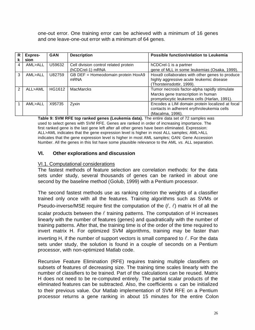
26

one-out error. One training error can be achieved with a minimum of 16 genesand one leave-one-out error with a minimum of 64 genes.

Rk

Expres-sion

GAN Description Possible function/relation to Leukemia

4 AML>ALL U59632 Cell division control related protein(hCDCrel-1) mRNA

hCDCrel-1 is a partnergene of MLL in some leukemias (Osaka, 1999).

3 AML>ALL U82759 GB DEF = Homeodomain protein HoxA9mRNA

Hoxa9 collaborates with other genes to producehighly aggressive acute leukemic disease(Thorsteinsdottir, 1999).

2 ALL>AML HG1612 MacMarcks Tumor necrosis factor-alpha rapidly stimulateMarcks gene transcription in humanpromyelocytic leukemia cells (Harlan, 1991).

1 AML>ALL X95735 Zyxin Encodes a LIM domain protein localized at focalcontacts in adherent erythroleukemia cells(Macalma, 1996).

Table 9: SVM RFE top ranked genes (Leukemia data). The entire data set of 72 samples wasused to select genes with SVM RFE. Genes are ranked in order of increasing importance. Thefirst ranked gene is the last gene left after all other genes have been eliminated. Expression:ALL>AML indicates that the gene expression level is higher in most ALL samples; AML>ALLindicates that the gene expression level is higher in most AML samples; GAN: Gene AccessionNumber. All the genes in this list have some plausible relevance to the AML vs. ALL separation.

VI. Other explorations and discussion

VI.1. Computational considerationsThe fastest methods of feature selection are correlation methods: for the datasets under study, several thousands of genes can be ranked in about onesecond by the baseline method (Golub, 1999) with a Pentium processor.

The second fastest methods use as ranking criterion the weights of a classifiertrained only once with all the features. Training algorithms such as SVMs orPseudo-inverse/MSE require first the computation of the (l, l) matrix H of all thescalar products between the l training patterns. The computation of H increaseslinearly with the number of features (genes) and quadratically with the number oftraining patterns. After that, the training time is of the order of the time required toinvert matrix H. For optimized SVM algorithms, training may be faster thaninverting H, if the number of support vectors is small compared to l. For the datasets under study, the solution is found in a couple of seconds on a Pentiumprocessor, with non-optimized Matlab code.

Recursive Feature Elimination (RFE) requires training multiple classifiers onsubsets of features of decreasing size. The training time scales linearly with thenumber of classifiers to be trained. Part of the calculations can be reused. MatrixH does not need to be re-computed entirely. The partial scalar products of theeliminated features can be subtracted. Also, the coefficients α can be initializedto their previous value. Our Matlab implementation of SVM RFE on a Pentiumprocessor returns a gene ranking in about 15 minutes for the entire Colon

27

dataset (2000 genes, 62 patients) and 3 hours on the Leukemia dataset (7129genes, 72 patients). Given that the data collection and preparation may takeseveral months or years, it is quite acceptable that the data analysis takes a fewhours.

All our feature selection experiments using various classifiers (SVM, LDA, MSE)indicated that better features are obtained by using RFE than by using theweights of a single classifier (see Section VI.2 for details). Similarly, better resultsare obtained by eliminating one feature at a time than by eliminating chunks offeatures. However, there are only significant differences for the smaller subset ofgenes (less than 100). This suggests that, without trading accuracy for speed,one can use RFE by removing chunks of features in the first few iterations andthen remove one feature at a time once the feature set reaches a few hundreds.This may become necessary if the number of genes increases to millions, as isexpected to happen in the near future.

The scaling properties of alternative methods that have been applied to other“feature selection” problems are generally not as attractive. In a recent reviewpaper (Blum, 1997), the authors mention that “few of the domains used to datehave involved more than 40 features”. The method proposed in (Shürmann,1996), for example, would require the inversion of a (n, n) matrix, where n is thetotal number of features (genes).

VI.2. Analysis of the feature selection mechanism of SVM-RFE

1) Usefulness of RFEIn this section, we question the usefulness of the computationally expensiveRecursive Feature Elimination (RFE). In Figure 5, we present the performance ofclassifiers trained on subsets of genes obtained either by “naively” ranking thegenes with (wi)2, which is computationally equivalent to the first iteration of RFE,or by running RFE. RFE consistently outperforms the naïve ranking, particularlyfor small gene subsets.

The naïve ranking and RFE are qualitatively different. The naïve ranking ordersfeatures according to their individual relevance. The RFE ranking is a featuresubset ranking. The nested feature subsets contain complementary features notnecessarily individually most relevant. This is related to the relevance vs.usefulness distinction (Kohavi, 1997).

The distinction is most important in the case of correlated features. Imagine, forexample, a classification problem with 5 features, but only 2 distinct features bothequally useful: x1, x1, x2, x2, x2. A naïve ranking may produce weight magnitudesx1(1/4), x1(1/4), x2(1/6), x2(1/6), x2(1/6), assuming that the ranking criterion givesequal weight magnitudes to identical features. If we select a subset of twofeatures according to the naïve ranking, we eliminate the useful feature x2 andincur possible classification performance degradation. In contrast, a typical run ofRFE would produce:

28

Figure 5: Effect of Recursive Feature Elimination (Colon cancer data). In this experiment, wecompared the ranking obtained by RFE with the naïve ranking obtained by training a singleclassifier and using the magnitude of the weights as ranking coefficient. We varied the number oftop ranked genes selected. Training was done on the entire data set of 62 samples. The curvesrepresent the leave-one-out success rate for the various feature selection methods, using anSVM classifier. The colors represent the classifier used for feature selection. Black: SVM. Red:Linear Discriminant Analysis. Green: Mean Squared Error (Pseudo-inverse). We do not representthe baseline method (Golub, 1999) since RFE and the naïve ranking are equivalent for thatmethod. The solid line corresponds to RFE. The dashed line corresponds to the naïve ranking.RFE consistently outperforms the naïve ranking, for small gene subsets.

first iteration x1(1/4), x1(1/4), x2(1/6), x2(1/6), x2(1/6),second iteration x1(1/4), x1(1/4), x2(1/4), x2(1/4)third iteration x2(1/2), x1(1/4), x1(1/4)fourth iteration x1(1/2), x2(1/2)fifth iteration x1(1)Therefore if we select two features according to RFE, we obtain both x1 and x2,as desired.

The RFE ranking is not unique. Our imagined run produced: x1 x2 x1 x2 x2,corresponding to the sequence of eliminated genes read backwards. Severalother sequences could have been obtained because of the symmetry of theproblem, including x1 x2 x2 x1 x2 and x2 x1 x2 x1 x2. We observed in realexperiments that a slight change in the feature set often results in a completelydifferent RFE ordering. RFE alters feature ordering only for multivariateclassification methods that do not make implicit feature orthogonalityassumptions. The method of (Golub, 1999) yields the same ordering for thenaïve ranking and RFE.

0123456789100.5

0.55

0.6

0.65

0.7

0.75

0.8

0.85

0.9

0.95

1

Leav

e-on

e-ou

t suc

cess

rat

e

SVM

MSELDA

log2(number of genes)

29

Figure 6: Feature selection and support vectors. This figure contrasts on a two dimensionalclassification example the feature selection strategy of “average case” type methods and that ofSVMs. The red and blue dots represent examples of class (-) and (+) respectively. The decisionboundary D(x)=0 separates the plane into two half planes D(x)<0 ⇒ x in class (-), and D(x)>0 ⇒ xin class (+). There is a simple geometric interpretation of the feature ranking criterion based onthe magnitude of the weights: for slopes larger than 45 degrees, the preferred feature is x1,otherwise it is x2. The example was constructed to demonstrate the qualitative difference of themethods. Feature x2 separates almost perfectly all examples with a small variance, with theexception of one outlier. Feature x1 separates perfectly all examples but has a higher variance.(a) Baseline classifier (Golub, 1999). The preferred feature is x2. (b) SVM. The preferred featureis x1.

x1

x2

D(x)=0

D(x)<0

D(x)>0

(a)

x1

x2

D(x)=0

D(x)<0

D(x)>0

(b)

30

2) Feature selection mechanism of SVMsIn the experimental section (Section V), we conjectured that SVMs have afeature selection mechanism relying on support vectors that distinguishes themfrom “average case” methods. In this section, we illustrate on an example whatsuch a mechanism could be.

In Figure 6, we constructed a two-dimensional classification example. The dotswere placed such that feature x2 separates almost perfectly all examples with asmall variance, with the exception of one outlier. Feature x1 separates perfectlyall examples but has a higher variance. We think of feature x1 as the relevantfeature (a cancer-related gene) and as feature x2 as the irrelevant feature (atissue composition related gene): most examples are very well separatedaccording to tissue composition, but one valuable outlier contradicts this generaltrend. The baseline classifier (Golub, 1999) prefers feature x2. But the SVMprefers feature x1.

Therefore the SVM feature selection critically depends on having clean datasince the outliers play an essential role. In our approach, the two problems ofselection of useful patterns (support vectors) and selection of useful features aretightly connected. Other approaches consider the two problems independently(Blum, 1997).

VI.3. Generalization of SVM RFE to the non-linear case and other kernelmethodsThe method of eliminating features on the basis of the smallest change in costfunction described in Section II.5 can be extended to the non-linear case and toall kernel methods in general (Weston, 2000-b). One can make computationstractable by assuming no change in the value of the α’s. Thus one avoids havingto retrain a classifier for every candidate feature to be eliminated.

Specifically, in the case of SVMs ((Boser, 1992), (Vapnik, 1998), (Cristianini,1999)), the cost function being minimized (under the constraints 0 ≤ αk ≤ C and

∑k

αk yk =0) is:

J = (1/2) α TH α – α T1,where H is the matrix with elements yhykK(xh,xk), K is a kernel function thatmeasures the similarity between xh and xk, and 1 is an l dimensional vector ofones. An example of such a kernel function is K(xh,xk)=exp(-γ ||xh-xk||2).To compute the change in cost function caused by removing input component i,one leaves the α’s unchanged and one re-computes matrix H. This correspondsto computing K(xh(-i), xk(-i)), yielding matrix H(-i), where the notation (-i) meansthat component i has been removed. The resulting ranking coefficient is:

DJ(i) = (1/2) α TH α – (1/2) α T H(-i) αThe input corresponding to the smallest difference DJ(i) shall be removed. Theprocedure can be iterated to carry out Recursive Feature Elimination (RFE).

31

In the linear case, K(xh,xk)=xh.xk and α TH α = ||w ||2. Therefore DJ(i)=(1/2)(wi)2.The method is identical the one we proposed and studied in the previoussections for linear SVMs.

Computationally, the non-linear kernel version of SVM RFE is a little moreexpensive than the linear version. However, the change in matrix H must becomputed for support vectors only, which makes it affordable for small numbersof support vectors. Additionally, parts of the calculation such as the dot productsxh.xk between support vectors can be cached.

We performed preliminary experiments on a classical example of non-linearclassification problem, the XOR problem, which indicate that the method ispromising. We added to a 2 by 2 two checker board 50 extra noisy dimensions,all 52 dimensions generated with uniform distribution on -0.5 to 0.5. We averagedperformance over 30 random trials with a polynomial kernel of degree 2,K(x,y)=(x.y+1)2. Using our feature ranking method we selected the top twofeatures. For 30 training examples the correct two features were selected 22/30times. For 40 training examples the correct two features were selected 28/30times. We also compared classification performance with and without featureselection (Table 10). The SVM performs considerably better with featureselection on this problem.

Training set size Top 2 features selected No feature selection30 0.1775 ± 0.1676 0.4691 ± 0.023340 0.1165 ± 0.1338 0.4654 ± 0.0236100 0.0350 ± 0.0145 0.4432 ± 0.02591000 0.0036 ± 0.0024 0.3281 ± 0.0218Table 10: Non-linear SVM RFE. Fifty extra noisy dimensions were added to a 2 by 2 twochecker board (XOR problem). All 52 dimensions were generated with uniform distribution on -0.5to 0.5. The table shows averaged performance and standard deviation on a test set of 500examples over 30 random trials using a polynomial classifier of degree 2.

The idea of keeping the α’s constant to compute DJ can be extended to themulti-class problem (Bredensteiner, 1999) other kernel methods such as KPCA(Schölkopf, 1998), non-classification problems such as regression, densityestimation (see e.g. Vapnik, 1998) and clustering (Ben-Hur, 2000). It is notlimited to RFE type of search. It can be used, for instance, for forward featureselection (progressively adding features), a strategy recently used, for example,in (Smola, 2000).

VI.4. Other SVM feature selection methods

1) Penalty-based methodsWe explored other methods of feature selection using SVMs. One idea is toformulate the optimization problem in a way that a large number of weights will

32

be forced to zero. We tried the following linear programming formulation of theproblem:

Minimize over wi, wi* and ξk

∑i

(wi + wi*) + C ∑k

ξk

subject to:yk[(w*-w).xk + b] ≥ 1 – ξk

wi > 0wi*> 0i=1…n, k=1…lwhere C is a positive constant (penalty parameter).Although the idea is quite attractive, we did not obtain in our experiment resultsthat matched the performance of SVM RFE. Similar ideas have been proposedand studied by other authors (Bradley, 1998-a and -b). One drawback of penalty-based methods is that the number of features chosen is an indirect consequenceof the value of the penalty parameter.

2) Feature scaling methodsThe magnitude of the weights of a linear discriminant function is a scaling factorof the inputs. The idea of ranking features according to scaling factors subject totraining therefore generalizes the scheme that we have been using. Non-lineardiscriminant functions such as neural networks and kernel methods canincorporate such scaling factors. Several authors ((Mukherjee, 2000)(Jebera, 2000), (Chapelle, 2000), (Weston, 2000-a)) have recently proposed andstudied feature selection methods for SVMs that incorporate scaling factors intothe kernel:

KA(x, y) = K(Ax, Ay)where A is a diagonal matrix of scaling factors a1, a2, …an. Training is performedby iterating:1) Optimize the α’s for a fixed A (regular SVM training).2) Optimize A for fixed α’s by gradient descent.There are various flavors of the method depending on which cost function isbeing optimized in step 2 and which optimization method is used.The scaling factors are used to assess feature relevance. It is possible to set athreshold on feature relevance or select a given number of most relevantfeatures.

In (Mukherjee, 2000), the authors report on the leukemia data (Golub, 1999) zeroerror with no rejects on the test set using the top 40 genes. They were able toclassify 32 of 34 cases correctly using 5 genes. In (Chapelle, 2000), the authorsachieve 1 error on the test set with 5 genes using the same data set. In (Weston,2000-a), the authors report on the Leukemia data zero error with 20 genes and 1error with 5 genes. On the colon cancer data (Alon, 1999), the same authorsreport 12.8% average error of 50 splits of the data into 50 training examples and12 test examples.

33

We note that the least relevant feature(s) could be eliminated and the processiterated as in RFE, but no results on this computationally expensive approachhave been reported.

One drawback of feature scaling methods is that they rely on gradient descent.As such, they are sensitive to the choice of the gradient step, prone to falling inlocal minima and may be slow for a large number of features.

3) Wrapper methods and other search techniquesSVM RFE improves feature selection based on feature ranking by eliminating theorthogonality assumptions of correlation methods. Yet, it remains a greedy sub-optimal method. It generates nested subsets of features. This means that theselected subset of m features is included in the subset of m+1 features. But,assume that we found a feature singleton that provides the best possibleseparation. There is no guarantee that the best feature pair will incorporate thatsingleton. Feature ranking methods miss that point.

Combinatorial search is a computationally intensive alternative to feature ranking.To seek an optimum subset of m features or less, all combinations of m featuresor less are tried. The combination that yields best classification performance (ona test set or by cross-validation) is selected. The classifier is used as a so-called“wrapper” in the feature selection process (Kohavi, 1997).

We tried to refine our optimum feature set by combinatorial search using SVMs ina wrapper approach. We started from a subset of genes selected with SVM RFE.We experimented with the leukemia data, using the training/test data split. Wecould easily find a pair of genes that had zero leave-one-out error and a verywide positive extremal margin. Yet, the error rate on the test set was very poor(13/34 errors).

The failure of these explorations and the success of RFE indicate that RFE has abuilt in regularization mechanism that we do not understand yet that preventsoverfitting the training data in its selection of gene subsets. Other authors havemade similar observations for other greedy algorithms (Kohavi, 1997). Placingconstraints on the search space undoubtedly contributes to reduce thecomplexity of the learning problem and prevent overfitting, but a more precisetheoretical formulation is still missing.

As a compromise between greedy methods and combinatorial search, othersearch methods could be used such as beam search or best first search (Kohavi,1997).

34

VII. Conclusions and future work

SVMs lend themselves particularly well to the analysis of broad patterns of geneexpression from DNA micro-array data. They can easily deal with a large numberof features (thousands of genes) and a small number of training patterns (dozensof patients). They integrate pattern selection and feature selection in a singleconsistent framework.

We proposed and applied the SVM method of Recursive Feature Elimination(RFE) to gene selection. We showed experimentally on two different cancerdatabases that taking into account mutual information between genes in the geneselection process impacts classification performance. We obtained significantimprovements over the baseline method that makes implicit orthogonalityassumptions. We also verified the biological relevance of the genes found bySVMs. The top ranked genes found by SVM all have a plausible relation tocancer. In contrast, other methods select genes that are correlated with theseparation at hand but not relevant to cancer diagnosis.

The RFE method was demonstrated for linear classifiers, including SVMs. Thissimple method allows us to find nested subsets of genes that lend themselveswell to a model selection technique that finds an optimum number of genes. Ourexplorations indicate that RFE is much more robust to data overfitting than othermethods, including combinatorial search.

Further work includes experimenting with the extension of the method to non-linear classifiers, to regression, to density estimation, to clustering, and to otherkernel methods. We envision that linear classifiers are going to continue to playan important role in the analysis of DNA micro-array because of the large rationumber of features over number of training patterns.

Feature ranking methods do not dictate the optimum number of features to beselected. An auxiliary model selection criterion must be used for that purpose.The problem is particularly challenging because the leave-one-out error by itselfis of little use since it is zero for a large number of gene subsets. Possible criteriathat we have explored include the number of support vectors and a combinationof the four metrics of classifier quality (error rate, rejection rate, extremal margin,and median margin) computed with the leave-one-out procedure. We have alsoexplored with adding penalties for large numbers of features, using bounds onthe expected error rate. Finding a good model selection criterion is an importantavenue of experimental and theoretical research.

Greedy methods such as RFE are known by experimentalists to be less prone tooverfitting than more exhaustive search techniques. A learning theoretic analysisof the regularization properties of SVM RFE remains to be done.

Finally, we have directed our attention to feature selection methods that optimizethe feature subset for a given family of classifier (e.g. linear discriminant). More

35

generally, the simultaneous choice of the learning machine and the featuresubset should be addressed, an even more complex and challenging modelselection problem.

Acknowledgements

The authors are grateful to the authors of Matlab code who made their sourcecode available through the Internet. Our implementation grew from code writtenby Steve Gunn (http://www.isis.ecs.soton.ac.uk/resources/svminfo) Dick DeRidder and Malcolm Slaneyhttp://valhalla.ph.tn.tudelft.nl/feature_extraction/source/svc/). We would also liketo thank Trey Rossiter for technical assistance and useful suggestions, and thereviewers for their thorough work.

Bibliography

(Aerts, 1996) Chitotriosidase - New Biochemical Marker. Hans Aerts. GauchersNews, March, 1996.

(Alizadeh, 2000) Distinct types of diffuse large B-cell lymphoma identified bygene expression profiling. Ash A. Alizadeh et al, Nature, Vol. 403, Issue 3,February, 2000.

(Alon, 1999) Broad patterns of gene expression revealed by clustering analysisof tumor and normal colon cancer tissues probed by oligonucleotide arrays. Alonet al, PNAS vol. 96 pp. 6745-6750, June 1999, Cell Biology. The data is availableon-line at http://www.molbio.princeton.edu/colondata.

(Aronson, 1999) Remodeling the Mammary Gland at the Termination of BreastFeeding: Role of a New Regulator Protein BRP39, The Beat, University of SouthAlabama College of Medecine, July, 1999.

(Ben Hur, 2000) A support vector method for hierarchical clustering. A. Ben Hur,D. Horn, H. Siegelman, and V. Vapnik. Submitted to NIPS 2000.

(Boser, 1992) An training algorithm for optimal margin classifiers. B. Boser, I.Guyon, and V. Vapnik. In Fifth Annual Workshop on Computational LearningTheory, pages 144--152, Pittsburgh, ACM. 1992.

(Blum, 1997) Selection of relevant features and examples in machine learning. A.Blum and P. Langley. Artificial intelligence, 97:245-271, 1997.

(Bradley, 1998-a) Feature selection via mathematical programming. P. Bradley,O. Mangasarian, and W. Street. Technical report to appear in INFORMS Journalon computing, 1998.

36

(Bradley, 1998-b) Feature selection via concave minimization and support vectormachines. P. Bradley and O. Mangasarian. In proc. 13th International Conferenceon Machine Learning, pages 82-90, San Francisco, CA, 1998.

(Bredensteiner, 1999) Multicategory classification for support vector machines. E.Bredensteiner and K. Bennett. Computational Optimizations and Applications,12, 1999, pp 53-79.

(Brown, 2000) Knowledge-based analysis of microarray gene expression data byusing support vector machines, Michael P. S. Brown, William Noble Grundy,David Lin, Nello Cristianini, Charles Walsh Sugnet, Terrence S. Furey, ManuelAres, Jr., and David Haussler. PNAS, Vol. 97, no. 1: 262–267, January, 2000.

(Chapelle, 2000) Choosing kernel parameters for support vector machines. O.Chapelle , V. Vapnik, O. Bousquet, and S. Mukherjee. AT&T Labs technicalreport. March, 2000.

(Cortes, 1995) Support Vector Networks. C. Cortes and V. Vapnik. MachineLearning, Vol. 20, no. 3: 273-297, September,1995.

(Cristianini, 1999) An introduction to support vector machines. N. Cristianini andJ. Shawe-Taylor. Cambridge University Press. 1999.

(Duda, 1973) Pattern classification and scene analysis. Richard O. Duda andPeter E. Hart. Wiley. 1973.

(Eisen, 1998) Cluster analysis and display of genome-wide expression patternsMichael B. Eisen, Paul T. Spellman, Patrick O. Brown and David Botstein. Proc.Natl. Acad. Sci. USA, Vol. 95, pp. 14863–14868, December 1998, Genetics.

(Fodor, 1997) Massively Parallel Genomics. S. A. Fodor. Science. 277:393-395,1997.

(Furey, 2000) Support Vector Machine Classification and Validation of CancerTissue Samples Using Microarray Expression Data. T. Furey, N. Cristianini, N.Duffy, D. Bednarski, M. Schummer, and D. Haussler. To appear inBioinformatics.

(Ghina, 1998) Altered Expression of Heterogeneous Nuclear Ribonucleoproteinsand SR Factors in Human, Claudia Ghigna, Mauro Moroni, Camillo Porta,Silvano Riva, and Giuseppe Biamonti, Cancer Research, 58, 5818-5824,December 15, 1998.

(Golub, 1999) Molecular Classification of Cancer: Class Discovery and ClassPrediction by Gene Expression Monitoring. Golub et al, Science Vol 286, Oct

37

1999. The data is available on-line athttp://www.genome.wi.mit.edu/MPR/data_set_ALL_AML.html.

(Guyon, 1992) Structural risk minimization for character recognition. I. Guyon, V.Vapnik, B. Boser, L. Bottou, and S.A. Solla. In J. E. Moody et al., editor,Advances in Neural Information Processing Systems 4 (NIPS 91), pages 471--479, San Mateo CA, Morgan Kaufmann. 1992.

(Guyon, 1996) Discovering informative patterns and data cleaning. I. Guyon, N.Matic , and V. Vapnik. In U.M. Fayyad, G. Piatetsky-Shapiro, P. Smyth, and R.Uthurusamy, editors, Advances in Knowledge Discovery and Data Mining, pages181--203. MIT Press. 1996.

(Guyon, 1998) What size test set gives good error rate estimates? I. Guyon, J.Makhoul, R. Schwartz, and V. Vapnik. PAMI, 20 (1), pages 52--64, IEEE. 1998.

(Guyon, 1999) SVM Application Survey:http://www.clopinet.com/SVM.applications.html.

(Harlan, 1991) The human myristoylated alanine-rich C kinase substrate(MARCKS) gene (MACS). Analysis of its gene product, promoter, andchromosomal localization. DM Harlan, JM Graff, DJ Stumpo, RL Eddy Jr, TBShows, JM Boyle and PJ Blackshear. Journal of Biological Chemistry, Vol. 266,Issue 22, 14399-14405, August, 1991.

(Hastie, 2000) Gene Shaving: a New Class of Clustering Methods for ExpressionArrays. T. Hastie, R. Tibshirani, M. Eisen, P. Brown, D. Ross, U. Scherf, J.Weinstein, A. Alisadeh, L. Staudt, and D. Botstein. Stanford technical report, Jan.2000.

(Jebara, 2000) Feature selection and dualities in maximum entropydiscrimination. T. Jebara and T. Jaakkola. In Uncertainty in Artificial Intelligence,2000.

(Karakiulakis, 1997) Increased Type IV Collagen-Degrading Activity inMetastases Originating from Primary Tumors of the Human Colon, Karakiulakis,G.; Papanikolaou, C.; Jankovic, S.M.; Aletras, A.; Papakonstantinou, E.; Vretou,E.; Mirtsou-Fidani, V. Invasion and Metastasis, Vol. 17, No. 3, 158-168, 1997.

(Kearns, 1997) . An experimental and theoretical comparison of model selectionmethods. Kearns M., Mansour Y., Ng A.Y., and Ron D. Machine Learning 27: 7–50. 1997.

(Kohavi, 1997) Wrappers for feature subset selection. Ron Kohavi and GeorgeJohn. In Artificial Intelligence journal, special issue on relevance, Vol. 97, Nos 1-2, pp. 273-324.

38

(LeCun, 1990) Optimum Brain Damage, Y. Le Cun, J.S. Denker, and S.A. Solla.In D. Touretzky Ed. Advances in Neural Information Processing Systems 2. Pp598-605, Morgan Kaufmann. 1990.

(Macalma, 1996) Molecular characterization of human zyxin. Macalma T, Otte J,Hensler ME, Bockholt SM, Louis HA, Kalff-Suske M, Grzeschik KH, von der AheD, Beckerle MC. Journal of Biological Chemistry. Vol. 271, Issue 49, 31470-31478, December, 1996.

(Mozer, 1999) Angiostatin binds ATP synthase on the surface of humanendothelial cells, Tammy L. Moser, M. Sharon Stack, Iain Asplin, Jan J. Enghild,Peter Højrup, Lorraine Everitt, Susan Hubchak, H. William Schnaper, andSalvatore V. Pizzo, PNAS, Vol. 96, Issue 6, 2811-2816, March 16, 1999,Cell Biology.

(Mukherjee, 2000) Support vector machine classification of microarray data. S.Mukherjee, P. Tamayo, D. Slonim, A. Verri, T. Golub, J.P. Messirov, and T.Poggio. AI memo 182. CBCL paper 182. MIT. Can be retrieved fromftp://publications.ai.mit.edu.

(Oliveira, 1999) Chronic Trypanosoma cruzi infection associated to colon cancer.An experimental study in rats. Enio Chaves de Oliveira. Resumo di Tese. Revistada Sociedade Brasileira de Medicina Tropical 32(1):81-82, jan-fev, 1999.

(Osaka, 1999) MSF (MLL septin-like fusion), a fusion partner gene of MLL, in atherapy-related acute myeloid leukemia with a t(11;17)(q23;q25). Osaka M,Rowley JD, Zeleznik-Le NJ, Proc Natl Acad Sci U S A. Vol. 96, Issue 11, 6428-33, May, 1999.

(Pavlidis, 2000) Gene functional Analysis from Heterogeneous Data. P. Pavlidis,J. Weston, J. Cai, and W. N. Grundy. Submitted for publication.

(Perou, 1999) Distinctive gene expression patterns in human mammaryepithelial cells and breast cancers, Charles M. Perou et al Proc. Natl. Acad. Sci.USA, Vol. 96, pp. 9212–9217, August 1999, Genetics.

(Schölkopf, 1998) Non-linear component analysis as a kernel eigenvalueproblem. B. Schölkopf, A. Smola, K.-R. Muller. Neural computation, vol. 10, pp.1299-1319, 1998.

(Shürmann, 1996) Pattern Classification. J. Shürmann. Wiley Interscience. 1996.

(Smola, 2000) Sparce greedy matrix approximation for machine learning. A.Smola and B. Schölkopf. Proceedings of the 17th international conference onmachine learning, pp 911-918. June, 2000.

39

(Thorsteinsdottir , 1999) The oncoprotein E2A-Pbx1a collaborates with Hoxa9 toacutely transform primary bone marrow cells. Thorsteinsdottir U, Krosl J, KroonE, Haman A, Hoang T, Sauvageau G. Molecular Cell Biology, Vol. 19, Issue 9,6355-66, September, 1999.

(Vapnik, 1998) Statistical Learning Theory. V. N. Vapnik. Wiley Interscience.1998.

(Walsh, 1999) Epidemiologic Evidence Underscores Role for Folate as Foiler ofColon Cancer. John H. Walsh, Section Editor. Gastroenterology News.Gastroenterology. 116:3-4 ,1999.

(Weston, 2000-a) Feature Selection for SVMs. J. Weston, S. Muckerjee, O.Chapelle, M. Pontil, T. Poggio, and V. Vapnik. Submitted to NIPS 2000.

(Weston, 2000-b) Feature selection for kernel machines using stationary weightapproximation. J. Weston and I. Guyon. In preparation.