general equilibrium analysis of the eaton–kortum model of

ARTICLE IN PRESS

Journal of Monetary Economics 54 (2007) 1726–1768

0304-3932/$ -

doi:10.1016/j

$We than

John Romali

participants i

University, B

referees for c

provided man�CorrespoE-mail ad

www.elsevier.com/locate/jme

General equilibrium analysis of the Eaton–Kortummodel of international trade$

Fernando Alvareza, Robert E. Lucas, Jr.b,�

aUniversity of Chicago and NBER, USAbUniversity of Chicago and Federal Reserve Bank of Minneapolis, USA

Received 25 July 2005; received in revised form 7 June 2006; accepted 25 July 2006

Available online 19 December 2006

Abstract

We study a variation of the Eaton–Kortum model, a competitive, constant-returns-to-scale

multicountry Ricardian model of trade. We establish existence and uniqueness of an equilibrium with

balanced trade where each country imposes an import tariff. We analyze the determinants of the

cross-country distribution of trade volumes, such as size, tariffs and distance, and compare a

calibrated version of the model with data for the largest 60 economies. We use the calibrated model

to estimate the gains of a world-wide trade elimination of tariffs, using the theory to explain the

magnitude of the gains as well as the differential effect arising from cross-country differences in pre-

liberalization tariff levels and country size.

r 2006 Elsevier B.V. All rights reserved.

Keywords: General equilibrium; Ricardian trade theory; Trade volume; Tariff policy

see front matter r 2006 Elsevier B.V. All rights reserved.

.jmoneco.2006.07.006

k Jonathan Eaton, Tim Kehoe, Sam Kortum, Ellen McGrattan, Sergey Mityakov, Casey Mulligan,

s, Kim Ruhl, Ed Prescott, Phil Reny, Rob Shimer, Nancy Stokey, Chad Syverson, Ivan Werning,

n the December, 2003, conference at Torcuato di Tella and seminar participants at Cornell, Boston

rown, Harvard, Minnesota and Chicago for helpful discussions. We thank the editor and several

lose reading and useful criticism. Constantino Hevia, Natalia Kovrijnykh, and Oleksiy Kryvtsov

y suggestions and able assistance.

nding author. Tel.: +1 773 702 8191; fax: +1 773 702 8490.

dresses: [email protected] (R.E. Lucas, Jr.).

ARTICLE IN PRESSF. Alvarez, R.E. Lucas, Jr. / Journal of Monetary Economics 54 (2007) 1726–1768 1727

1. Introduction

Eaton and Kortum (2002) have proposed a new theory of international trade, aneconomical and versatile parameterization of the models with a continuum of tradeablegoods that Dornbusch et al. (1977) and Wilson (1980) introduced many years ago. In thetheory, constant-returns producers in different countries are subject to idiosyncraticproductivity shocks. Buyers of any good search over producers in different countries forthe lowest price, and trade assigns production of any good to the most efficient producers,subject to costs of transportation and other impediments. The gains from trade are larger,the larger is the variance of individual productivities, which is the key parameter in themodel.

The model shares with those of the ‘‘new trade theory’’ the important ability to dealsensibly with intra-industry trade: trade in similar categories of goods between similarlyendowed countries.1 But unlike the earlier theory, the Eaton–Kortum (2002) model iscompetitive, involving no fixed costs and no monopoly rents. Of course, fixed costs andmonopoly rents are present in reality, but theories based on competitive behavior are muchsimpler to calibrate and permit the use of a large body of general equilibrium theory tohelp in analysis.

One aim of this paper is to restate the economic logic of a variation of theEaton–Kortum model of trade in a particular general equilibrium context. In the nextsection, we will introduce the basic ideas using a closed economy with a productiontechnology of the Eaton–Kortum type. In Section 3, we define an equilibrium withbalanced trade in a world with many countries, each one imposing import tariffs. Section 4gives sufficient conditions for this equilibrium to exist, and addresses the problem ofdetermining whether this equilibrium is unique and of finding an algorithm to compute it.

A second goal of the paper is to find out whether the cross-country distribution of tradevolumes generated by a model of this type is consistent with the behavior of volumes in thedata. In Section 5, we calibrate some of the main parameters of the theory. Section 6discusses some instructive special cases that are simple enough to work out by hand. Usingestimates from Section 5, we examine the implications of these special cases of the theoryfor the volume of trade and the way that trade volume behaves as a function of size, andcompare these implications to data on total GDP and trade volumes for the 60 largesteconomies. Sections 7 and 9 go over the same ground numerically with more realisticassumptions. In these two sections we apply the algorithm described in Section 4, calibratethe model to the observed distribution of GDPs and the relative prices of tradeables tonon-tradeable goods, and introduce heterogeneity in transportation costs and tariff rates.

Our normative goal is to use the quantitative theory to estimate the welfare gains fromhypothetical trade liberalizations. Comparisons between free trade and autarchy arecarried out in Sections 6. Section 8 studies the optimal tariff policy of a small economy. InSection 8 we also calculate the effects of a world-wide liberalization in which everycountry’s tariffs are set to zero. We use the theory to explain the magnitude of the averagegains of trade, as well as differential effects arising from cross-country differences in pre-liberalization tariff levels and country size. Section 9 describes the effects on these estimates

1See, for example, Ethier (1979, 1982), Krugman (1979), Helpman (1981), and the Helpman and Krugman

(1985) monograph. Baxter (1992) argues that competitive, Ricardian models are equally capable of dealing

realistically with intra-industry trade.

ARTICLE IN PRESSF. Alvarez, R.E. Lucas, Jr. / Journal of Monetary Economics 54 (2007) 1726–17681728

of calibrating the model to fit relative price differences across countries. Conclusions arecontained in Section 10.

2. Preferences, technology, and closed economy equilibrium

The Eaton–Kortum model is Ricardian, with a continuum of goods produced under aconstant-returns technology. The new idea is a two-parameter probabilistic model thatgenerates the input requirements for producing each good. It will be useful to introducethis model of a technology in the simpler context of a single, closed economy beforeturning to the study of a model of a world of n countries in Section 3.We develop a purely static model in which labor is the only primary (non-produced)

factor of production. There are L consumers, and each is endowed with one unit of labor.All production is subject to constant returns, and we conduct the entire analysis of theclosed economy in per capita terms. There is a single, produced final good, c, which is theonly good valued by consumers. We use c for utility as well.A continuum of intermediate goods are produced, and these goods affect production

symmetrically via a Spence–Dixit–Stiglitz (SDS) aggregate. Total factor productivity(TFP) levels vary across goods. As in Eaton and Kortum (2002), we model the inverses ofthese TFP levels (‘‘costs’’) as random variables, independent across goods, with a commondensity f. Since intermediate goods differ only in their costs, in this sense, it is convenientto name each intermediate good by its cost draw, x40, and to speak of ‘‘good x.’’Let qðxÞ be production of intermediate good x, and denote the production of the SDS

aggregate by q. Then

q ¼

Z 10

qðxÞ1�1=ZfðxÞdx

� �Z=ðZ�1Þ. (2.1)

The labor endowment is allocated over final goods production, sf , and production of theintermediates, sðxÞ, x40:

sf þ

Z 10

sðxÞfðxÞdxp1. (2.2)

The intermediates qf and qmðxÞ are allocated over the same uses:

qf þ

Z 10

qmðxÞfðxÞdxpq.

The production technologies are Cobb–Douglas. For final goods,

c ¼ saf q1�af . (2.3)

For intermediate good x,

qðxÞ ¼ x�ysðxÞbqmðxÞ1�b. (2.4)

Throughout we follow Eaton–Kortum (2002) and assume that the density f isexponential with parameter l: x� expðlÞ. These x draws are then amplified in percentageterms by the parameter y. 2 (The random variables x�y then have a Frechet distribution.)

2We are using y for the parameter that Eaton and Kortum call 1=y, so that in this paper a larger y means a

larger variance in individual productivities.


It is important to emphasize that these cost draws x are economy-wide effects. Anyone isfree to produce any specific good, and every producer of that good has access to the sameproduction technology (2.4), with the same stochastic intercept x�y, as other producers do.Since (2.4) is a constant-returns technology the number of firms producing any good willbe indeterminate, but whatever that number is, no single producer has any market powerand all prices will be set at marginal cost, equivalent to minimum unit cost. This is true forfinal goods production as well.

Denote the wage rate by w, the price of final goods by p, the prices of individualtradeables by pðxÞ, and the price of the intermediate aggregate by pm. Cost minimizingbehavior of all producers will ensure that equilibrium prices satisfy

p ¼ a�að1� aÞ�1þawap1�am , (2.5)

pðxÞ ¼ Bxywbp1�bm , (2.6)

where

B ¼ b�bð1� bÞ�1þb,

and

pm ¼ lZ 10

e�lxpðxÞ1�Z dx

� �1=1�Z

. (2.7)

We can use (2.6) and (2.7) to solve for pm as a multiple of the wage. We have

pm ¼ lZ 10

e�lxðBxywbp1�bm Þ

1�Z dx

� �1=ð1�ZÞ¼ Bwbp1�b

m l�yZ 10

e�zzyð1�ZÞ dz

� �1=ð1�ZÞ, ð2:8Þ

using the change of variable z ¼ lx. We write Aðy; ZÞ, or sometimes just A, for

Aðy; ZÞ ¼Z 10

e�zzyð1�ZÞ dz

� �1=ð1�ZÞ.

The integral in brackets is the Gamma function GðxÞ, evaluated at the argumentx ¼ 1þ yð1� ZÞ. Convergence of the integral requires

1þ yð1� ZÞ40, (2.9)

which we assume to hold throughout this paper.3

In terms of A, (2.8) implies

pm ¼ ðABÞ1=bl�y=bw. (2.10)

Substituting from (2.10) back into (2.5) and (2.6) then yields the prices of individualintermediate goods

pðxÞ ¼ Að1�bÞ=bB1=bxyl�yð1�bÞ=bw, (2.11)

3If Z were too large to satisfy (2.9), the integral in (2.8) would not converge. Economically, this would mean

unbounded production of the tradeable aggregate, as labor is concentrated on goods where x is near zero (where

x�y is very high). Changes in the parameter Z will affect the units in which tradeables are measured, and hence

relative prices that depend on these units. The allocation of labor and materials between the two sectors is

independent of the value of Z. (See footnote 4.)


and of final goods

p ¼ a�að1� aÞ�1þaðABÞð1�aÞ=bl�yð1�aÞ=bw. (2.12)

Notice that all these prices, p, pm, and pðxÞ, are different multiples of the wage rate w. Thisis a labor theory of value: everything is priced according to its labor content.Given these solutions for equilibrium prices, equilibrium quantities are readily

calculated, using the familiar Cobb–Douglas constant share formulas. We turn, in thenext section, to a model of international trade, in which the intermediate goods aretradeable (at a cost) and neither labor nor final goods can move. This fact will completelyalter the determination of the price pm of the tradeable, intermediate aggregate, but withineach country, nothing else will change. The pricing functions (2.5) and (2.6) will continue toobtain, and the calculation of quantities, given prices, will be the same as in this closedeconomy section.

3. General equilibrium

We turn to a version of the Eaton–Kortum (2002) model, and consider an equilibrium ina world of n countries, all with the structure described in Section 2, in which trade isbalanced. Let total labor endowments be L ¼ ðL1; . . . ;LnÞ, where Li is the total units oflabor in i, measured in efficiency units. Labor is not mobile. The exponential distributionsthat define each country’s technology have the parameters l ¼ ðl1; . . . ; lnÞ. We use w ¼

ðw1; . . . ;wnÞ for the vector of wages in the individual countries. Preferences and thetechnology parameters y, b, a, and Z, are common to all countries. The structure ofproduction in each country is exactly as described in Section 2, except that nowintermediate goods are traded—and will now be called tradeables—subject to transporta-tion costs and tariffs.Transportation costs are defined in physical, ‘‘iceberg’’ terms: we assume that one unit of

any tradeable good shipped from j to i results in kij units arriving in i. Interpreting theterms kij as representing costs that are proportional to distance, it is natural to assume thatkij40, kijp1, with equality if i ¼ j, kij ¼ kji for all i; j, and

kijXkikkkj for all i; j; k. (3.1)

We also want to consider tariffs that distort relative prices but do not entail a physicalloss of resources. In practice, trade barriers take many forms, but here we consider only flatrate tariffs levied by country i on goods imported from j, and where the proceeds arerebated as lump sum payments to the people living in i. Define oij to be the fraction of eachdollar spent in i on goods made in j that arrives as payment to a seller in j.In the closed economy analysis of Section 2 we exploited the assumptions of competition

and constant returns to solve for all equilibrium prices as multiples of the wage w, withcoefficients depending only on the technology. With this done, we can then calculateequilibrium quantities. This same two-stage procedure can be applied to the case of manycountries, though of course each stage is more complicated.A new notation for the commodity space is needed. Let x ¼ ðx1; . . . ; xnÞ be the vector of

technology draws for any given tradeable good for the n countries. We refer to ‘‘goodx’’, as before, but now x 2 Rn

þ. Assume that these draws are independent across countries,


so that the joint density of x is

fðxÞ ¼Yn

i¼1

li

!exp �

Xn

i¼1

lixi

( ).

Use qiðxÞ for the consumption of tradeable good x in country i, and qi for consumption in i

of the aggregate,

qi ¼

ZqiðxÞ

1�1=ZfðxÞdx

� �Z=ðZ�1Þ.

(HereRdenotes integration over Rn

þ:Þ Let piðxÞ be the prices paid for tradeable good x byproducers in i. Let

pmi ¼

ZpiðxÞ

1�ZfðxÞdx

� �1=ð1�ZÞ(3.2)

be the price in i for a unit of the aggregate.The tradeable good x ¼ ðx1; . . . ; xnÞ is available in i at the unit prices

Bxy1w

b1p

1�bm1

1

ki1oi1; . . . ;Bxy

nwbnp1�b

mn

1

kinoin

,

which reflect both production costs (labor and intermediate inputs) and transportation andtariff costs. All producers in i buy at the same, lowest price:

piðxÞ ¼ Bminj

wbj p

1�bmj

kijoij

xyj

" #. (3.3)

Note that without assumption (3.1), the right side of (3.3) would not necessarily be theleast cost way of obtaining good x in country i.

The price index pmi of tradeables in i must be calculated country by country. We derivean expression for pmi from (3.2) and (3.3). The derivation uses two well-known propertiesof the exponential distribution:

x� expðlÞ and k40 ) kx� explk

� �(3.4)

and

x and y independent; x� expðlÞ; y� expðmÞ,

and z ¼ minðx; yÞ ) z� expðlþ mÞ. ð3:5Þ

From (3.2), we have

p1�Zmi ¼

ZpiðxÞ

1�ZfðxÞdx, (3.6)

and note that the right side is the expected value of the random variable piðxÞ1�Z. From

(3.3)

piðxÞ1=y¼ B1=y min

j

wb=yj p

ð1�bÞ=ymj

ðkijoijÞ1=y

xj

" #.


Property (3.4) implies that zj � wb=yj p

ð1�bÞ=ymj ðkijoijÞ

�1=yxj is exponentially distributed withparameter

cij ¼wbj p

1�bmj

kijoij

!�1=ylj, (3.7)

and property (3.5) implies that z � minj zj is exponentially distributed with parameterPnj¼1cij . Applying (3.4) again, this proves that piðxÞ

1=y is exponentially distributed withparameter

m ¼ B�1=yXn

j¼1

cij.

It then follows from (3.6) that

p1�Zmi ¼ m

Z 10

uyð1�ZÞe�mu du.

Using the change of variable z ¼ mu, we have that

p1�Zmi ¼ m�yð1�ZÞ

Z 10

e�zzyð1�ZÞ dz

¼ m�yð1�ZÞA1�Z,

where A ¼ Aðy; ZÞ is the constant defined in Section 2. Then

pmiðwÞ ¼ ABXn

j¼1

cij

!�y� AB

Xn

j¼1

wbj pmjðwÞ

1�b

kijoij

!�1=ylj

0@ 1A�y, (3.8)

i ¼ 1; . . . ; n.We view (3.8) as n equations in the prices pm ¼ ðpm1; . . . ; pmnÞ, to be solved for pm as a

function of the wage vector w. It is the same formula as (7) and (9) in Eaton and Kortum(2002). Notice that the country identifier i appears on the right side of (3.8) only via theparameters kij and oij.Next we calculate the tradeables expenditure shares for each country i: the fraction Dij of

country i’s per capita spending pmiqi on tradeables that is spent on goods from country j.Economically, the total spending in i on goods from j is just

pmiqiDij ¼

ZBij

piðxÞ qiðxÞfðxÞdx,

where Bij � Rnþ is the set on which j attains the minimum in (3.3). Using (3.2) and (3.3),

this integral can be evaluated to obtain the expression (3.10) (below) for Dij .One can also show that the Dij will simply be the probabilities that for a particular good

x, the low price vendors for buyers in i are sellers in j. These probabilities can be calculateddirectly, using a third fact about exponential distributions:

x and y independent; x� expðlÞ and y� expðmÞ

) Prfxpyg ¼l

lþ m. ð3:9Þ


From (3.3) we have

Dij ¼ Prwbj p

1�bmj

kijoij

xyj pmin

kaj

wbkp

1�bmk

kikoik

xyk

" #( )

¼ Prwbj p

1�bmj

kijoij

!1=y

xjpminkaj

wbkp

1�bmk

kikoik

!1=y

xk

24 358<:9=;.

By (3.4), the random variable on the left of the inequality is exponential with parameter cij .By (3.4) and (3.5), the random variable on the right is exponential with parameterP

kaj cik, and the two are obviously independent. Thus (3.9) implies

Dij ¼cijPn

k¼1 cik

¼ ðABÞ�1=ywbj pmjðwÞ

1�b

pmiðwÞkijoij

!�1=ylj. (3.10)

Note thatP

jDij ¼ 1.We now impose trade balance. Under this assumption, the dollar payments for

tradeables flowing into i from the rest of the world must equal the payments flowing out ofi to the rest of the world. Firms in i spend a total of Lipmiqi dollars on tradeables, includingboth transportation costs and tariff payments. Of this amount,

Lipmiqi

Xn

j¼1

Dijoij

reaches sellers in all countries (including i itself). The rest is collected in taxes, and rebatedas a lump sum to consumers in i.

Buyers in j spend a total of LjpmjqjDji dollars for tradeables from i, but of this total only

LjpmjqjDjioji

reaches sellers in i. The rest remains in j, as rebated tax receipts. Trade balance thenrequires that the condition

Lipmiqi

Xn

j¼1

Dijoij ¼Xn

j¼1

LjpmjqjDjioji (3.11)

must hold. Notice that the term LipmiqiDiioii—country i’s spending on home-producedtradeables—appears on both sides of (3.11). Cancelling thus yields the usual definition oftrade balance: payments to foreigners equal receipts from foreigners.

Our strategy for constructing the equilibrium in this world economy draws on theanalysis of a single, closed economy in Section 2. As in that section, we first note that allprices in all countries can be expressed in terms of wages. In the present case, wages are avector w ¼ ðw1; . . . ;wnÞ and we express the coefficients cij as functions of w and pm, andthen use the n equations (3.8) to solve for the prices pm ¼ ðpm1; . . . ; pmnÞ as a function pmðwÞ

of wages. This problem is the subject of Theorem 1 in the next section. The impact of therest of the world on the behavior of individual producers in i is entirely determined by theseprices pmi. With tradeable prices expressed as functions of wages (and of the tax rates andother parameters involved in (3.8)), (3.10) expresses the expenditure shares Dij as functionsof wages and tax rates, too. Then (3.11) can be viewed as an equation in wages w and thevector q of tradeables consumption per capita.


We first consider the implications of trade balance in the absence of taxes: oij ¼ 1 for alli; j. In this case, the trade balance condition (3.11) reduces to

Lipmiqi ¼Xn

j¼1

LjpmjqjDji. (3.12)

The share of tradeables in the production of the final good is, in this case,

1� a ¼Lipmiqf i

Liwi

,

using the fact that in the absence of indirect taxes, GDP equals national income:Lipici ¼ Liwi. The share of tradeables in the production of tradeables is

1� b ¼Lipmiðqi � qf iÞ

Lipmiqi

,

using the fact—trade balance, again—that the value of tradeables produced must equal thevalue of tradeables used in production. These two share formulas together imply

bLipmiqi ¼ ð1� aÞLiwi. (3.13)

Applying this fact to both sides of the trade balance condition (3.12) and cancelling, weobtain

Liwi ¼Xn

j¼1

LjwjDjiðwÞ; i ¼ 1; . . . ; n. (3.14)

We do not need to restrict the transportation cost parameters kij to reduce (3.11) to (3.14)because the effects of these costs are entirely captured in (3.8).Theorem 2 in the next section provides conditions that ensure that (3.14) has a solution

w, but since our objective is to be able to analyze the effects of changes in tariff policies, wecannot stop with this special case. Nor can we make use of the share formulas to simplify(3.11) in the general case: the presence of indirect business taxes breaks the equality ofGDP and national income that we used to derive (3.14).To deal with the general case, we need to start from (3.11), not (3.12), and we need to

adapt the share formulas to incorporate taxes. This adaptation is primarily an accountingexercise, based on the national income and product accounts for a country i.Table 1 provides the accounts for country i, viewed as a three sector economy. All

entries are in dollars. The left side gives value added in each sector; the right side gives

Table 1

Value added in services Labor income in services

Lipici � Lipmiqf i Liwisf i

Value added in tradeables Labor income in tradeablesPj LjpmjqjDjioji � Lipmiqmi Liwið1� sf iÞ

Value added in importing Indirect business taxes

Lipmiqi � Lipmiqi

Pj Dijoij Lipmiqi

PjaiDijð1� oijÞ

GDP Total labor income plus indirect taxes

Lipici Liwi þ Lipmiqi

Pjai Dijð1� oijÞ


factor payments (labor payments plus indirect business taxes). Two of these sectors areservices (final goods) and tradeables. The third is an importing sector, in which firms buytradeable goods from both home and foreign producers, pay import duties to their owngovernment, and resell the goods to home producers. This is a constant-returns, free-entryactivity, so of course selling prices must be marked up exactly to cover the taxes. If oij ¼ 1,the entries for this sector would be zero in both columns. To verify that the three sectorvalue-added terms sum to GDP, one needs to use the trade balance condition (3.11).

Based on these accounts, the derivation of (3.14) from (3.11) can be paralleled, and it canbe shown that (3.11) implies

Liwið1� sf iÞ ¼Xn

j¼1

Lj

wjð1� sf jÞ

Fj

Djioji, (3.15)

where

sf i ¼a½1� ð1� bÞFi�

ð1� aÞbFi þ a½1� ð1� bÞF i�(3.16)

and

Fi ¼Xn

j¼1

Dijoij. (3.17)

Here sf i is labor’s share in the production of final goods and Fi is the fraction of country i’sspending on tradeables that reaches producers (as opposed to the home government). Bothare functions of w as are the shares Dij. Details are provided in Appendix A.

We view solving these equations as finding the zeros of an excess demand system ZðwÞ:

ZiðwÞ ¼1

wi

Xn

j¼1

Lj

wjð1� sf jðwÞÞ

F jðwÞDjiðwÞoji � Liwið1� sf iðwÞÞ

" #. (3.18)

We sum up this section in the following definition.

Definition. An equilibrium is a wage vector w 2 Rnþþ such that ZiðwÞ ¼ 0 for i ¼ 1; . . . ; n,

where the functions pmiðwÞ satisfy (3.8), the functions DijðwÞ satisfy (3.10), the functionsFiðwÞ satisfy (3.17), and the functions sf iðwÞ satisfy (3.16).

Given an equilibrium wage vector w and the tradeable aggregate prices pmiðwÞ in eachcountry i, all other equilibrium prices and quantities can be calculated as we have describedin Section 2.

4. Existence, uniqueness, and computation of equilibrium

The economy we analyze is specified by the technology parameters a, b, Z, and y,common to all countries, the country-specific populations and technology levels L ¼

ðL1; . . . ;LnÞ and l ¼ ðl1; . . . ; lnÞ, the transportation parameters ½kij�, and the taxparameters ½oij �. All these numbers are strictly positive. Moreover, we impose:

Assumptions (A). (A1) a; bo1,(A2) 1þ yð1� ZÞ40, and for some numbers k and o,(A3) 0o kpkijp1 and 0oopoijp1.


Under these assumptions, we study the existence and uniqueness of solutions to theexcess demand system (3.18). Before turning directly to these issues, Theorem 1characterizes the function pmð�Þ : R

nþþ ! Rn

þ relating tradeable goods prices to wagerates, defined implicitly by Eqs. (3.8). Then Theorem 2 shows that the excess demandsystem (3.18) satisfies the sufficient conditions for a theorem on the existence ofequilibrium in an n-good exchange economy. Theorem 3 gives one set of assumptions thatimplies that this solution is unique.

Theorem 1. Under Assumptions (A), for any w 2 Rnþþ there is a unique pmðwÞ that satisfies

(3.8). For each i, the function pmiðwÞ is

(i)
continuously differentiable on Rnþþ,
(ii)
homogeneous of degree one, (iii) strictly increasing in w, (iv) strictly decreasing in the parameters kij and oij, and
(v)
satisfies the bounds
pmðwÞppmiðwÞppmðwÞ,

for all w 2 Rnþþ, where

pmðwÞ ¼AB

ko

� �1=b Xn

j¼1

w�b=yj lj

!�y=b(4.1)

and

pmðwÞ ¼ ðABÞ1=bXn

j¼1

w�b=yj lj

!�y=b. (4.2)

The proof of Theorem 1 is provided in Appendix B.To prove that an equilibrium exists, we will apply an existence theorem for an exchange

economy with n goods to the demand system ZðwÞ defined in (3.18).

Theorem 2. Under Assumptions (A) there is a w 2 Rnþþ such that

ZðwÞ ¼ 0.

Proof. We verify that ZðwÞ has the properties

(i)
ZðwÞ is continuous, (ii) ZðwÞ is homogeneous of degree zero, (iii) w � ZðwÞ ¼ 0 for all w 2 Rn
þþ (Walras’s Law),
(iv) for k ¼ maxj Lj40, ZiðwÞ4� k for all i ¼ 1; . . . ; n and w 2 Rn
þþ, and
(v) if wm ! w0, where w0a0 and w0
i ¼ 0 for some i, then

maxjfZjðw

mÞg ! 1. (4.3)

Then the result will follow from Proposition 17.C.1 of Mas-Colell et al. (1995, p. 585).(i) The continuity of pmi is implied by part (i) of Theorem 1. The continuity of the

functions Dij is then evident from (3.10). The functions Fi defined in (3.17) are continuous,


and are uniformly bounded from below by o. The functions sfi defined in (3.16) arecontinuous. The continuity of Z then follows from (3.18).

(ii) From Theorem 1, pmi is homogeneous of degree one. Then (3.10) implies that the Dij

are homogeneous of degree zero, and it is immediate that Fi, sf i , and Zi all have thisproperty.

(iii) To verify Walras’s Law, restate (3.18) as

wiZi ¼Xn

j¼1

Ljwjð1� sf jÞ1

F j

Djioji � Liwið1� sf iÞ

and sum over i to getXn

i¼1

wiZi ¼Xn

i¼1

Xn

j¼1

Ljwjð1� sf jÞ1

F j

Djioji �Xn

i¼1

Liwið1� sf iÞ

¼Xn

j¼1

Ljwjð1� sf jÞXn

i¼1

1

F j

Djioji �Xn

i¼1

Liwið1� sf iÞ ¼ 0

using (3.14).The proofs of parts (iv) and (v) are in Appendix A. &

We next establish a sufficient condition for the equilibrium be unique. To do so, we addto Assumptions (A) the assumption that the import duties oij levied by country i areuniform over all source countries j, so that we write oij ¼ oi for iaj and oii ¼ 1. Then wehave:

Theorem 3. If Assumptions (A) hold, if oij ¼ oi for all iaj, and if

ðko Þ2=yX1� b, (4.4)

aXb, (4.5)

and

1� opy

a� b, (4.6)

there is exactly one solution to ZðwÞ ¼ 0 that satisfiesPn

i¼1 wi ¼ 1.

Proof. In Appendix B, we use the results from Theorem 1, (iii) and (v), to establish that Z

has the gross substitute property

qZiðwÞ

qwk

40 for all i; k; iak for all w 2 Rþþ:. (4.7)

(Since Z is homogeneous of degree zero, (4.7) will imply that

qZiðwÞ

qwi

40 for all i for all w 2 Rþþ:Þ

Then the result will follow from Proposition 17.F.3 of Mas-Colell et al. (1995, p. 613). &

One can see that (4.4) and (4.6) are satisfied if the tariff and transportation costs aresmall enough. For the parameter values for a, b, and y proposed in Section 5, condition(4.4) is satisfied if tariffs and transportation cost are both less than 2.5%. Condition (4.5) is


easily satisfied for the benchmark calibration presented later on. Of course, conditions(4.4)–(4.6) are sufficient, not necessary, conditions for the gross substitute property toobtain. For the case of two countries, it can be shown that (4.6) alone is sufficient. Ournumerical experience also confirms that the gross substitute property holds under muchwider conditions than (4.4)–(4.6), including quite high tariff and transportation costs.We finish this section by discussing the algorithm that we use to compute equilibrium.

The gross substitute property applied in Theorem 3 suggests the use of a discrete timeanalogue of the continuous time tatonnement process. Let Dw be defined as

Dw ¼ w 2 Rnþ:Xn

i¼1

wiLi ¼ 1

( ).

Then we define the function T, mapping Dw into itself as follows:

TðwÞi ¼ wið1þ nZiðwÞ=LiÞ; i ¼ 1; . . . ; n, (4.8)

where n is an arbitrary constant satisfying n 2 ð0; 1�. Notice that ZiðwÞ=Li is country i’slabor excess demand per unit of labor, so the operator T prescribes that the percentageincrease in country i’s wage be in proportion to a scaled version of country i’s excessdemand. To see that T : Dw ! Dw, note first that TðwÞiX0 if 1þ nZiðwÞ=LiX0, since Zi isbounded below by �Li by part (iv) of Theorem 2. Note second that for any w 2 DwXn

i¼1

TðwÞiLi ¼X

i

wi 1þ nZi

Li

� �Li ¼

Xn

i¼1

wiLi þ nXn

i¼1

wiZiðwÞ ¼ 1,

where the last equality uses Walras’ Law. To calculate TðwÞ numerically, one first needs tocalculate pmðwÞ, the solution to (3.8). We used an algorithm based on the contractionproperty used to prove Theorem 1.This function T is closely related to a continuous time version of the tatonnement

process. To see this, interpret T dynamically as giving the value TðwÞ to wðtþ nÞ wheneverwðtÞ takes the value w. Then (4.8) becomes

1

wiðtÞ

wiðtþ nÞ � wiðtÞ

n¼

ZiðwðtÞÞ

Li

.

Letting n! 0, we obtain

d logwiðtÞ

dt¼

ZiðwðtÞÞ

Li

. (4.9)

If Z satisfies the gross substitute property, the differential (4.9) converges globally to theunique equilibrium wage. A proof can be constructed by showing that LðwÞ ¼maxifZiðwÞ=Lig is a Lyapounov function for this system. In our computationalexperiments, we found that setting the parameter n of (4.9) equal to one always producedmonotone convergence, in the sense of sequences with decreasing Lyapounov functionsLðwÞ.

5. Calibration

The quantitative exercises presented below require estimated values for the parametersZ; a, b, and y, which are assumed to be common across economies, the matrices ½kij � and


½oij � that describe transportation costs and tariff policies, the endowmentsL ¼ ðL1; . . . ;LnÞ, and the technology parameters l ¼ ðl1; . . . ; lnÞ.

The value of the substitution parameter Z used in forming the tradeables aggregate doesnot affect any of the results reported below. 4 (See footnote 3 on this counterintuitiveresult.)

For a and b, we use 0.75 and 0.5, respectively. The theory divides production into twocategories: tradeables and non-tradeables (final goods). We classify agriculture, mining,and manufacturing as the ‘‘tradeable’’ sectors. In the theory b is the share of labor in thetotal value of tradeables produced, and a is the fraction sf i of employment in the non-tradeable sector. To calibrate the parameters a and b, we think of the primary factor Li as‘‘labor-plus-capital’’ or perhaps as ‘‘equipped labor’’, and identify wiLi with total valueadded, not just compensation of employees. Thus we use data on value added, as well as onthe distribution of employment and capital to calibrate a and b.

Here we discuss the evidence used for our choice of a: Using the BEA input–outputtables for the U.S. for 1996–1999, the value-added share of agriculture, mining, andmanufacturing sectors was about 0.2 which corresponds to a ¼ 0.8. Using employmentshares would yield a ¼ 0:82, while using fixed capital shares yields a ¼ 0:73: The UnitedNations Common Database for 1993 reports value added in the tradeable sectorsaveraging around 0.3 for the OECD countries, and levels ranging to 0.5 and higher forpoorer countries. The OECD input–output tables for 1990 imply a ¼ 0:72 for the OECDcountries. In short, 0.75 seems a reasonable value for a in the industrialized world,although it overstates the importance of non-tradeables for economies that are stillsubstantially pre-industrial. We use a ¼ 0:75 throughout this paper.

We now turn to the evidence used for the calibration of b. Using the BEA input–outputtables for the U.S. for 1996–1999, the ratio of value added in manufacturing to the totalvalue of production in this sector was about 0.38. This figure can be compared to the UN(UNIDO Industrial Statistics database) estimate of a world average value of 0.38 inmanufacturing for 1998. The OECD input–output table for 1990 gives an average of 0.38in agriculture, mining, and manufacturing. Since the labor share in most services is higher,including tradeable services in total tradeables would require a higher value of b. In theWorld Development Indicators data for 1996–1999, trade in goods was about 77% of totaltrade (exports plus imports over two) in goods and services for the U.S. and it was about80% on average for the countries listed in Table 2. Using the U.S. input–output table for1997, the average of the ratio of value added to gross product across all sectors, weightedby the share of each sector in U.S. exports, is 0.5. Based on these considerations, we useb ¼ 0:5 throughout this paper.

We use values of y in the range ½0:1; 0:25�, with 0.15 being our preferred value based onthe following information. The parameter y describing the variability of the nationalidiosyncratic component to productivity is central in quantitative applications of thetheory. The Eaton and Kortum specification implies a set of aggregate demands for goodsproduced by different countries. Demand functions of the same form can be derived fromthe assumption that each country has a CES utility function where goods produced indifferent countries appear as differentiated commodities, as in the Armington aggregationspecification. The connection between these two parameterizations, based on the bilateral

4The parameter Z does not affect the expenditure shares Dij , and so does not affect the variables Fi and si , and

so does not affect equilibrium wages.

ARTICLE IN PRESS

Table 2

Data and simulation results

Country name Size GDP as

% of world

GDP

Trade volume

Imports/GDP

Relative price.

Consumption/

mach. &

equipt.

Tariff (in %)

Mean across

goods

Welfare gain

of eliminating

tarrifs, in

percent

Per capita

GDP PPP

adjusted

U:S: ¼ 1

Y i [1] Vi [2] Pi [3] 100� ð1�OiÞ

[4]

[5] Y i [6]

United States 27.99 0.10 1.37 5.40 0.15 1.00

Japan 15.69 0.08 1.65 5.48 0.25 0.83

Germany 7.35 0.27 1.48 5.86 0.41 0.76

ROW 5.25 0.32 0.70 11.49 0.20 0.10

France 4.86 0.24 1.55 5.86 0.52 0.73

UK 4.30 0.28 1.28 5.86 0.56 0.70

Italy 3.85 0.25 1.27 5.86 0.59 0.71

China 2.86 0.22 0.70 ðÞ 18.58 0.47 0.10

Brazil 2.29 0.09 1.00 13.73 0.42 0.23

Canada 2.06 0.33 1.30 5.10 0.84 0.82

Spain 1.93 0.26 1.35 5.86 0.79 0.56

Mexico 1.40 0.29 0.72 14.26 0.56 0.26

India 1.34 0.13 0.70 ðÞ 33.44 2.79 0.07

Australia 1.32 0.17 1.13 5.30 0.94 0.76

Netherlands 1.31 0.48 1.51 5.86 0.89 0.75

Russia 1.09 0.28 0.48 12.47 0.63 0.24

Argentina 0.94 0.11 1.02 12.40 0.66 0.39

Switzerland 0.91 0.31 1.70 0.68 1.56 0.88

Belgium 0.85 0.73 1.61 5.86 0.99 0.80

Sweden 0.80 0.39 1.61 5.86 1.00 0.71

Austria 0.72 0.35 1.57 5.86 1.02 0.79

Turkey 0.61 0.25 0.62 12.20 0.75 0.21

Indonesia 0.59 0.32 0.60 9.88 0.81 0.10

Denmark 0.58 0.35 1.50 5.86 1.05 0.82

Hong Kong 0.52 1.39 1.70 0.00 1.74 0.76

Norway 0.50 0.36 1.67 4.04 1.24 0.90

Thailand 0.49 0.49 0.64 18.00 0.91 0.21

Poland 0.47 0.27 0.65 15.55 0.81 0.25

Saudi Arabia 0.47 0.36 0.70ðÞ 12.48 0.78 0.37

South Africa 0.47 0.24 0.70 ðÞ 8.30 0.92 0.29

Finland 0.41 0.34 1.39 5.86 1.10 0.70

Greece 0.40 0.19 1.08 5.86 1.10 0.48

Portugal 0.36 0.34 0.97 5.86 1.11 0.50

Israel 0.32 0.39 1.65 7.55 1.00 0.60

Iran 0.32 0.21 0.48 4.90 1.21 0.18

Colombia 0.31 0.19 0.70 ðÞ 11.70 0.85 0.20

Venezuela, RB 0.29 0.24 0.71 12.28 0.84 0.20

Malaysia 0.29 1.00 0.70 ðÞ 9.18 0.93 0.26

Singapore 0.29 1.62 2.02 0.16 1.78 0.67

Ireland 0.26 0.63 1.29 5.86 1.14 0.72

Egypt 0.25 0.22 0.22 27.60 2.05 0.11

Philippines 0.25 0.48 0.67 11.22 0.88 0.12

Chile 0.23 0.29 0.82 10.25 0.91 0.28

Pakistan 0.20 0.18 0.76 39.90 5.16 0.06

New Zealand 0.19 0.26 1.29 4.84 1.25 0.61

F. Alvarez, R.E. Lucas, Jr. / Journal of Monetary Economics 54 (2007) 1726–17681740

ARTICLE IN PRESS

Table 2 (continued )

Country name Size GDP as

% of world

GDP

Trade volume

Imports/GDP

Relative price.

Consumption/

mach. &

equipt.

Tariff (in %)

Mean across

goods

Welfare gain

of eliminating

tarrifs, in

percent

Per capita

GDP PPP

adjusted

U:S: ¼ 1

Y i [1] Vi [2] Pi [3] 100� ð1�OiÞ

[4]

[5] Y i [6]

Peru 0.18 0.16 0.72 13.30 0.88 0.15

Czech Republic 0.18 0.60 0.52 7.04 1.09 0.43

Algeria 0.16 0.27 0.70 ðÞ 24.60 1.63 0.16

Hungary 0.15 0.46 0.52 13.42 0.89 0.35

Ukraine 0.15 0.47 0.24 10.20 0.94 0.12

Bangladesh 0.14 0.15 0.68 21.30 1.27 0.05

Romania 0.12 0.31 0.38 16.03 0.95 0.21

Morocco 0.11 0.30 0.50 30.77 2.68 0.11

Nigeria 0.11 0.41 0.61 24.06 1.58 0.03

Vietnam 0.08 0.25 0.28 15.15 0.94 0.06

Belarus 0.08 0.62 0.30 12.63 0.92 0.20

Kazakhstan 0.07 0.40 0.37 1.15 1.71 0.16

Slovak Rep. 0.06 0.64 0.43 6.88 1.14 0.32

Tunisia 0.06 0.45 0.40 31.17 2.77 0.18

Sri Lanka 0.05 0.41 0.57 7.67 1.09 0.10

Simple average 1.67 0.370 0.94 11.26 1.12 0.41

Weighted

average

0.210 7.62 0.50

Sources: [1]: Share in world GDP. GDP in current dollars. From WDI 2002 cdRom, average 1994–2000. [2]:

0:5ðexportsþ importsÞ=GDP, all in current dollars. From WDI 2002 cdRom, average 1994–2000. [3]: Price of

machinery and equipment relative to consumption, from benchmark PWT year 1996. Average of other countries

for ROW. The countries marked with ðÞ are not in the 1996 PWT benchmark, so we use the average for the other

countries. [3] displays the reciprocal of this number. [4]: Average 1996–2000 ad valorem tariff rate, simple average

across products, from Dollar and Kraay, using World Bank database ‘‘Data on Trade and Imports Barriers’’,

when available. When it is not available, indicated as *, import duties/imports from WDI 2002. Average of other

59 countries for ROW. [5]: Calculations described in Section 8, Figs. 6 and 7. [6]: Penn World Table average

1994–2000. The weighted averages are GDP weighted for trade volume and welfare gains, and weighted by

imports for tariffs.

F. Alvarez, R.E. Lucas, Jr. / Journal of Monetary Economics 54 (2007) 1726–1768 1741

gravity formula, is y ¼ 1=ðs� 1Þ, where s is the Armington elasticity. Eaton and Kortum(2002, Sections 3–5) estimate y using bilateral trade data as well as prices of individualgoods. They obtain estimates in the range 0.08–0.28, with their preferred value beingy ¼ 0:12. Anderson and van Wincoop (2004) survey analogous bilateral, gravity-typeestimates of the Armington substitution elasticity. They conclude, based on several studies,that a reasonable range is s 2 ½5; 10�, which corresponds to y 2 ½0:11; 0:25�. Based on thesefindings, we report numerical experiments based on y values of 0:1, 0:15, and 0:25. 5

For many simulations we use a value of k ¼ 0:75, applied symmetrically to pairs i; j

with iaj, based on the following information. Gravity equation estimates often estimate

5More recently, Broda andWeinstein (2005, Table 5) have estimated import weighted elasticities ðsÞ for the U.S.

of 10.35 for the period 1972–1988 and of 5.36 for the period 1990–2001.


jointly y as well as trade cost (transportation costs plus tariffs and other artificial barriers).For instance, the Eaton and Kortum trade cost estimates corresponding to y ¼ 0:12 rangefrom 28% for neighboring countries up to 66% for distant pairs. Such high estimated‘‘border effects’’ are a common feature of estimates obtained using gravity equations, assummarized by Anderson and van Wincoop (2004) and Feenstra (2004, Chapter 5). Suchindirect statistical evidence, using distance measures, the presence or absence of commonborders, and the like, can support k values as low as 0.65. Anderson and van Wincoop(2004) also report direct evidence of transportation costs—freight charges—for the U.S. onthe order of 4% using trade weights and 11% simple averaging. Considering imputed timecosts on cargo in transit may add 9%. Such direct estimates applied to the world at largesupport an estimate of k ¼ 0:9. Our choice of k ¼ 0:75 for the symmetric case is acompromise between these two types of estimates.6

Some direct evidence on tariff costs is given in column (4) of our Table 2, describedbelow. They range from 5% or less for wealthy economies (which account for almost alltrade) to as high as 40% for some poor ones. Values like this show up in many studies.Most experts think that non-tariff barriers are at least as important, but they are hard toquantify. Anderson and van Wincoop (2004) review evidence from OECD countries,where non-tariff barriers are estimated to be equivalent to an 8% tariff. For manysimulations we assume the value o ¼ 0:9 applied symmetrically to all foreign suppliers.Neither the endowments L ¼ ðL1; . . . ;LnÞ nor the technology parameters l ¼ ðl1; . . . ; lnÞ

can be observed directly, and the problem of inferring their values from characteristics wecan observe will be a focus of Sections 7 and 9. Here we simply describe the limited,aggregate data set we use for this and other purposes.We use the 2002 WDI cdRom to assemble a cross-section of the 59 economies with

the largest total GDPs. These countries and the variables measured for each are listed inTable 2. We also include a residual, rest-of-world category (with 5% of world GDP),treated as the 60th economy. For each country, five variables are recorded, along with theutility gains from a simulated tariff reform that will be described in Section 8.Column (1) is total GDP, denoted by Y ¼ ðY 1; . . . ;Y nÞ. These are IMF-based nominal

values, converted to U.S. dollars at market exchange rates (where available). They are noton a purchasing power parity basis. In the table they are expressed as fractions of totalworld GDP. These flows and all the import and export flows that we used were averagedover the years 1994–2000 in order to reduce the importance of trade imbalances and yearto year fluctuations, about which the theory evidently has nothing to say.Column (2) is trade volume, denoted by V ¼ ðV1; . . . ;V nÞ, defined as the average of the

values of imports and exports, also from the 2002 WDI cdRom, divided by GDP. Bothimports and exports are defined to include services as well as goods.Column (3) reports the ratio of the consumption goods deflator for each country to an

index of the prices of machinery and equipment, from the 1996 benchmark year in thePenn World Table. We will use them as observations P ¼ ðP1; . . . ;PnÞ on the pricesðp1=pm1; . . . ; pn=pmnÞ in the theory.Column (4) lists estimates of average 1996–2000 import tariff rates for each country.

These are unweighted averages of ad valorem tariffs applied to different commodities.They are available in the World Bank database ‘‘Data on Trade and Import Barriers,’’ and

6In regressions reported in Section 7 we use pair-specific values of kij based on estimates of the effect of the

distance between countries i and j.


are described in Dollar and Kraay (2004). (For the three countries for which we do nothave tariff data, indicated by asterisks, we substituted tariffs from a second source: ratiosof import duties to imports, from WDI 2002. For the residual ROW, we used the averageof the rest of the column.)

Column (5) contains simulation results that are discussed in Section 8. Column (6) is a1994–2000 average of per capita GDP, on a purchasing power basis, from the Penn WorldTable. This last series is not used in any of the calculations reported below, but will aid ininterpreting some of the results.

6. Examples

The algorithm proposed in Section 4 makes it easy to compute equilibria with manycountries, differing arbitrarily, but it will be instructive to work through some examplesfirst that are simple enough to solve by hand. We derive the predictions of special cases ofthe theory for the behavior of trade volumes and the gains from trade, as measured by theeffects of changes in trade on real consumption.

For future reference, we start with the derivation of some useful formulas for tradevolumes and gains, under the assumption—used also in Theorem 3—that tariffs areuniform: oij ¼ oi for all iaj. We first derive expressions for the value of imports I i and thevolume of trade vi, defined as the ratio of the value of imports to GDP. The value ofimports I i is the fraction of tradeable expenditures bought abroad,

I i ¼ Lipmiqi

Xjai

Dij.

Specializing the price and share formulas we used in Section 3 to deriving the basicequilibrium condition (3.14), we find that for this uniform tariff case,

vi ¼I i

Lipici

¼ð1� aÞ

bðDii=ð1�DiiÞ þ oiÞ þ 1� oi

. (6.1)

Notice that ð1� aÞ=b is an upper bound for vi.Using this formula, we consider first the case of costless trade: kij ¼ oij ¼ 1, all i; j. This

is the analogue of the zero-gravity case analyzed in Section 4.4 of Eaton and Kortum(2002). We solve for each country’s wages wi, the prices of non-tradeable goods relative totradeables pi=pmi, the shares in world GDP Liwi=

PjLjwj, and the volume of trade vi, all as

functions of the parameters Li and li. With costless trade every country buys theintermediate inputs from the same lowest cost producer, so the pmi are the same for allcountries with the common value

pm ¼ ðABÞ1=bXn

j¼1

w�b=yj lj

!�y=b.

Inserting this information into (3.10) yields

DijðwÞ ¼Xn

k¼1

w�b=yk lk

!�1w�b=yj lj. (6.2)

Notice that the expenditure shares Dij do not depend on the identity i of theimporter. With o ¼ 1, (3.16) and (3.17) imply sf i ¼ a, and the excess demand functions


(3.18) can now be written as

ZiðwÞ ¼1� ab

� � Xn

j¼1

DijðwÞ

wi

Ljwj � Li

!.

Equating ZiðwÞ to 0 and applying (6.2), we solve for equilibrium wages

wi ¼ pli

Li

� �y=ðbþyÞ

, (6.3)

where the parameter p, which does not depend on i, will be set by whatever normalizationwe choose for w. (Compare to Eaton and Kortum (2002, equation (22)).)Setting p ¼ 1, total GDP for country i is

Liwi ¼ Lb=ðbþyÞi ly=ðbþyÞi , (6.4)

a geometric mean of productivity in tradeables li and labor in efficiency units Li. Noticethat if y ¼ 0, so that there is no variation of productivities, then country i’s GDP Liwi issimply Li: The price of the final non-tradeable goods relative to tradeable goods in countryi is given by

pi

pm

¼ a�að1� aÞ�1þali

Li

� �ay=ðbþyÞ

p�am , (6.5)

so that countries with high productivity li in tradeables have a high relative price of non-tradeables.We use this example to compute gains of trade by comparing the real value of final

consumption in the costless-trade case with the one in autarchy. To this end, denote by ci0

and pm0 the real consumption and price of aggregate tradeable in the costless-trade case,and likewise use ci and pmi for the autarchy case. Normalizing country i’s wage wi ¼ 1 inboth cases, we have that

ci0

ci

¼pmi

pm0

� �1�a

. (6.6)

Using (6.3) and (6.4) into the expression for pm0 ¼ pm derived above, and using (2.10) forpmi we obtain

logci0

ci

� �¼ ð1� aÞ

yblog

Pnj¼1wjLj

wiLi

!, (6.7)

where wjLj denotes country j’s GDP in the costless-trade equilibrium.The volume of trade vi in the costless trade case is given by

vi ¼1� abð1�DiiÞ ¼

1� ab

1�LiwiPj Ljwj

!. (6.8)

Our second example explores a different special case. We next study a symmetricequilibrium with equal sized countries Li ¼ L ¼ 1, identical technologies, li ¼ l, anduniform transportation costs and tariffs, described by

kij ¼ k and oij ¼ o if iaj


and kii ¼ oii ¼ 1. In these circumstances, there will be a common equilibrium wagewi ¼ w, all i. We normalize it to w ¼ 1. Everyone will face the same tradeables price pm,and (3.8) can be solved for

pm ¼ðABÞ1=b

ð1þ ðn� 1ÞðkoÞ1=yÞy=bly=b. (6.9)

The price of final goods is given by (2.12), which with w ¼ 1 and pm given by (6.9) yields

p ¼a�að1� aÞ�1þa ðABÞð1�aÞ=b

½1þ ðn� 1ÞðkoÞ1=y�yð1�aÞ=blyð1�aÞ=b. (6.10)

With w ¼ 1, (3.10) implies

Dij ¼ðkoÞ1=y

1þ ðn� 1ÞðkoÞ1=y

for iaj. Then applying (6.1), the imports/GDP ratio v equals

v ¼1� ab

ðn� 1ÞðkoÞ1=y

1þ ð1þ bo� oÞðn� 1ÞðkoÞ1=y=b. (6.11)

Nominal GDP per capita in this example is

pc ¼ 1þ Ið1� oÞ ¼ 1þ vpcð1� oÞ,

with v given by (6.11), and consumption, or utility, per unit of labor, is given by

c ¼1

1� vð1� oÞ1

p. (6.12)

We calculate the utility gain from eliminating a tariff o. Denote by c; I , and p the levelsof consumption, imports, and the consumption price corresponding to a tariff o and byc0; I0, and p0 the values corresponding to the case of no tariff: o ¼ 1. Then using (6.10)

c0

c¼ ½1� vð1� oÞ�

1þ ðn� 1Þk1=y

1þ ðn� 1ÞðkoÞ1=y

!yð1�aÞ=b

. (6.13)

We use Eqs. (6.11) and (6.13) to derive an expression for the gain L � logðc0=cÞ of goingfrom pure autarchy, o ¼ 0, to costless trade, k ¼ o ¼ 1. Specializing (6.12) to theautarchy-costless-trade comparison, we get

L � logðc0=cÞ ¼yð1� aÞ

blogðnÞ. (6.14)

In the last section we argued that the values a ¼ 0:75 and b ¼ 0:5 are empiricallyreasonable, at least for the high income countries. Using the value 0.15 for y, (6.14) thenimplies the gain estimate

L ¼ ð0:075Þ logðnÞ.

We can think of n in (6.14) as the ratio of world GDP to the home country’s, so thattaking values from Table 2, n ¼ 3:6ffi 1=0:28 for the United States, n ¼ 6:2 for Japan, andn ¼ 170 for Denmark. In percentage terms, this formula implies benefits of 10% ofconsumption for the U.S., 14% for Japan, and 38% for Denmark. These are fantasy


calculations—even ideally free trade is not costless trade—but they give useful upperbounds for the magnitude of gains we will be discussing in the rest of the paper.Next we return to the case of positive transportation costs and tariffs, retaining

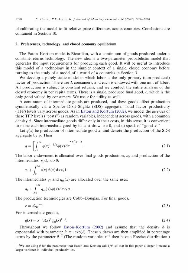
symmetry. The properties of the volume and welfare gain functions defined in (6.11) and(6.12)–(6.14) are illustrated in Figs. 1 and 2. In both figures we used the values a ¼ 0:75,b ¼ 0:5, k ¼ 0:75 and o ¼ 0:9. In Fig. 1, the values of y are varied, as shown. In Fig. 2,y ¼ 0:15.Fig. 1 shows the gains of eliminating a tariff corresponding to o ¼ 0:9 for three values of

y. As expected, the gains from eliminating a 10% tariff are far smaller than the gains (6.14)of moving from autarchy. Notice too that the gains in Fig. 1 are not always decreasing inthe size of the country: this is due to the effect of the revenue from the tariff. As formula(6.13) makes clear, there are two effects of eliminating a tariff (setting o ¼ 1). One is toreduce the price of the final, non-tradeable consumption good (that is, to increase p=p0).The other is that tariff revenues are lost. These effects have opposing effects on welfare,and are stronger if n is large (i.e. if countries are small). The first effect must dominate—eliminating the tariff must be welfare improving—but the welfare gain need not decreasemonotonically in n. We also computed the gains from eliminating a tariff for different ovalues (not shown in Fig. 1). Holding y fixed at 0.15, the difference in the welfare gainsfrom eliminating a 30% versus a 20% tariff is smaller than the difference between

0.1 0.15 0.2 0.25 0.3 0.350

0.1

0.2

0.3

0.4

0.5

0.6

0.7

0.8

0.9

1

WE

LF

AR

E G

AIN

IN

PE

RC

EN

T: lo

g d

iffe

rence in c

onsum

ption x

100

COUNTRY SIZE: fraction of world GDP

θ = 0.1

θ = 0.15

θ = 0.25

0.05

ω= 0.9κ= 0.75β= 0.5α= 0.75

Parameters

Fig. 1. Welfare gains from eliminating a 10% tariff. Three values of dispersion y.

ARTICLE IN PRESS

-8 -7 -6 -5 -4 -3 -2 -10

0.2

0.4

0.6

0.8

1

1.2

1.4

1.6

1.8

IMP

OR

T T

O G

DP

RA

TIO

COUNTRY SIZE: log of fraction of world GDP

θ = 0.15

ω = 0.9

κ = 0.75

β = 0.5

α = 0.75

Parameters

Singapore

Hong Kong

Malaysia

USA

Japan

Belgium

Ukraine

Bangladesh

Germany

Argentina

Fig. 2. Volume of trade.


eliminating a 40% versus a 30% tariff. For countries that are 5% of world GDP orsmaller, the gains from eliminating a 30% tariffs are about 6%.

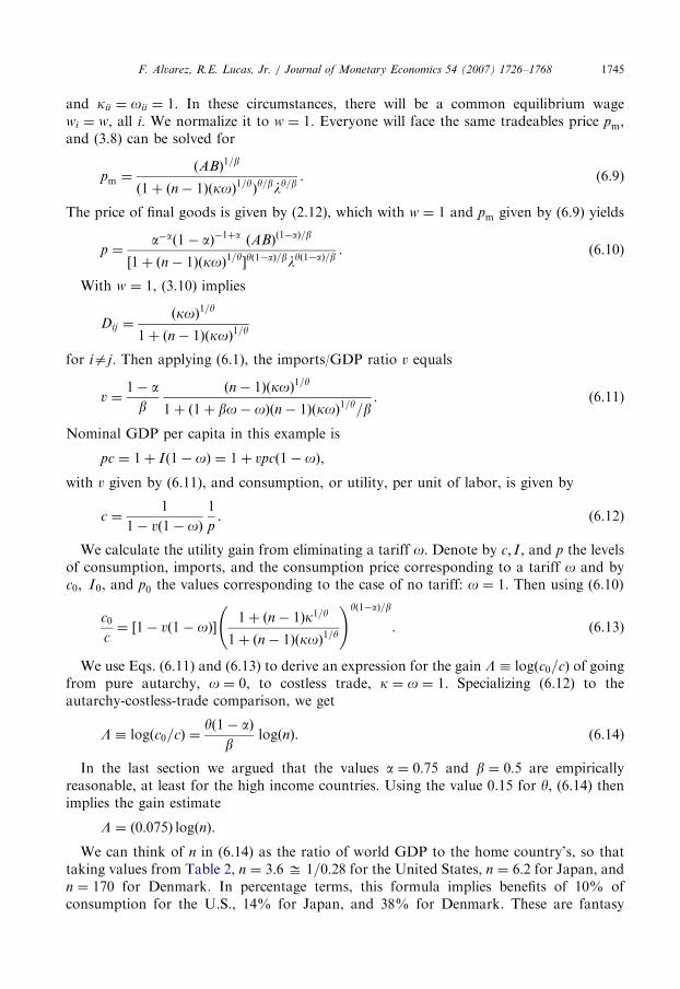
Fig. 2 plots the relation between the volume of trade, (6.11), measured as the ratio ofimport value to GDP, and the size of the economy, measured as the log of the economy’sGDP relative to the world total. The volume of trade is decreasing in size, and is boundedabove by the ratio of ð1� aÞ to ð1� ð1� bÞoÞ, which equals 0.45 for our benchmarkparameter values and o ¼ 0:9. Small economies have trade volumes that nearly attain thebound. We have also experimented varying the value of o between 0.7 and 1 (not shown inFig. 2). The effects of variations in o are large for economies of all sizes: for an economythat is 5% of world GDP, trade volume increases from 10% to 27%, as tariffs aredecreased from 30% to 10%.

Figs. 1 and 2 refer to symmetric world economies, where all economies have the samesize and technology levels. These are not cross-sections. The scatter of points in Fig. 2 areGDPs, Y i, and import to GDP ratios, V i, for 60 large countries: columns (1) and (2) inTable 2. These data are a cross-section. But the continuous curve on the picture iscalculated for a symmetric world, with a 10% tariff (o ¼ 0:9) just as in Fig. 1.

The data and all of the parameter values used to compute the theoretical curve in Fig. 2have all been discussed in Section 5. No adjustments have been made to fit the curve to thedata. The theoretical curve reproduces the negative relation between trade volume and size


in the data, but implies a slightly higher average trade volume than the average implied bythe data.In a world with very different national policies toward trade one would not expect equal

trade volumes at each GDP level, even if the assumptions underlying the construction ofFig. 2 were correct: the points should not lie on the theoretical curve. If the theory wereaccurate, the rich economies with more or less free trade—roughly, the OECD—should benear the curve, and the protectionist economies should fall below it by varying amounts.There are also four striking outliers in the figure: Hong Kong, Singapore, Malaysia, and

Belgium, with trade volumes much higher than others’, and much higher than ourtheoretical upper bound. It is a characteristic of port cities that a high volume of goodspasses through, counted as imports when they enter and exports when they leave.Countries in which such ports are important would appear as ‘‘low b’’ countries in ourparameterization, so it is possible that relaxing the assumption that b is uniform acrosseconomies would yield a better fit of the volume-size curves in Figs. 2 and 4, below.7

7. Volume of trade

The algorithm described in Section 4 lets us replace the theoretical curve in Fig. 2, basedon an assumption of symmetry, with the volume predictions of the general theory,calibrated to fit the actual distribution of economies by size. In addition, the general theorylets us incorporate other kinds of international differences—for example, differences intariff policies—into the trade volume predictions. We do this in this section, in two ways.Once the assumption of identical countries is dropped there is no reason for equilibrium

wages to be equal, and if they are not, observed GDPs Y cannot be taken as directobservations on equipped labor endowments L. Even without tariff distortions, Y i will bethe product wiLi, and neither w nor L can be directly inferred from observations on Y.What can be done about this depends on what other data are used.The simplest calibration method uses the theory to infer w and L from the data on Y

only. To do this, it seems a natural starting point to think of the parameter li in anycountry as proportional to that country’s equipped labor endowment Li. That is, weassume that if country 1 has twice the labor endowment of country 2, country 1 will alsohave twice as many ‘‘draws’’ from the distribution of productivities. With exponentiallydistributed productivities, this means l1 ¼ 2l2, and in general, that the vector l isproportional to the endowment vector L. This assumption of uniform ratios li=Li surelyhas more appeal than assuming uniform levels li. In the latter case, there would beenormous diseconomies of size: Denmark would be the low cost producer of as manygoods as the United States is, but with its much smaller workforce, Danish wage rates

7There is some evidence supporting this interpretation of the outliers in Fig. 2 as low-b port cities. The UN

Statistics Division (Commodity Trade Statistics Database: COMTRADE) collects data on re-exports of goods—

exports of goods that have been imported with no local value added—for 50 countries, 10 of which are in our 60

country data set. Of the four outlying high-volume countries in Fig. 2, only Hong Kong has re-export data. Hong

Kong reports that goods re-exports averaged about 85% of total goods exports during 1994–1999. Since goods

exports were about 86% of total exports, removing re-exports from total exports would lead to a reduction in the

estimated trade volume in Hong Kong from 1.4 to 1:4� ð0:14þ 0:86� 0:15Þ ¼ 0:38, or to about the level of the

theoretical curve in Fig. 2. For the other 50 countries in the COMTRADE data set, re-exports are less than 10%

of goods exports, and for most countries they are less than 1% of the total.


would be bid up to much higher levels than wages in the U.S.8 Of course, these are not theonly possibilities.

Under this assumption, the equilibrium condition

Zðw;L; lÞ ¼ 0, (7.1)

written so as to emphasize the dependence of the excess demand system Z on L and l, isspecialized to Zðw;L; kLÞ ¼ 0. The choice of the constant k is just a matter of the unitschosen for tradeables and labor input. We set it equal to one:

Zðw;L;LÞ ¼ 0. (7.2)

A second set of equations in the variables w and L is given by the GDP-equals-nationalincome conditions

L � bwðw;LÞ ¼ Y , (7.3)

where bwiðw; lÞ is wi adjusted for indirect taxes using the functions sf i and Fi of theequilibrium wage vector defined in (3.16) and (3.17):

bwiðw; lÞ ¼ wi 1þð1� sf iðw; lÞÞð1� Fiðw; lÞÞ

bF iðw; lÞ

� �. (7.4)

(Notice that without tariffs, oi ¼ 1 and bwiðw; lÞ ¼ wi.) We view (7.2) and (7.3) as 2n

equations in the pair ðw;LÞ, given the data Y.We describe the algorithm used to solve (7.2)–(7.3). Define wðl;LÞ to be the function

that solves (7.1). Its values can be calculated using the algorithm described in Section 4.Define j by

jiðLÞ ¼Y ibwiðwðL;LÞ;LÞ

�Xn

j¼1

Y jbwjðwðL;LÞ;LÞ. (7.5)

Then jmaps the n-dimensional simplex Dn into itself, and if L is a fixed point of j, the pairðwðL;LÞ;LÞ satisfies (7.2)–(7.3). We located a fixed point by iterating using (7.5), applyingthe algorithm from Section 4 to compute w at each iteration, from an initial guess for L.In practice, this algorithm always converged to a fixed point.9

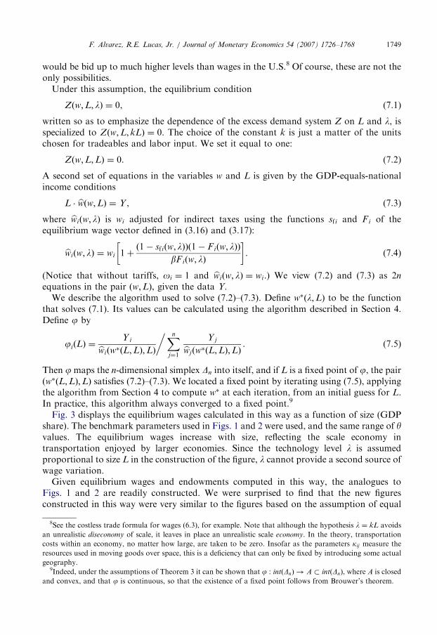
Fig. 3 displays the equilibrium wages calculated in this way as a function of size (GDPshare). The benchmark parameters used in Figs. 1 and 2 were used, and the same range of yvalues. The equilibrium wages increase with size, reflecting the scale economy intransportation enjoyed by larger economies. Since the technology level l is assumedproportional to size L in the construction of the figure, l cannot provide a second source ofwage variation.

Given equilibrium wages and endowments computed in this way, the analogues toFigs. 1 and 2 are readily constructed. We were surprised to find that the new figuresconstructed in this way were very similar to the figures based on the assumption of equal

8See the costless trade formula for wages (6.3), for example. Note that although the hypothesis l ¼ kL avoids

an unrealistic diseconomy of scale, it leaves in place an unrealistic scale economy. In the theory, transportation

costs within an economy, no matter how large, are taken to be zero. Insofar as the parameters kij measure the

resources used in moving goods over space, this is a deficiency that can only be fixed by introducing some actual

geography.9Indeed, under the assumptions of Theorem 3 it can be shown that j : intðDnÞ ! A � intðDnÞ, where A is closed

and convex, and that j is continuous, so that the existence of a fixed point follows from Brouwer’s theorem.

ARTICLE IN PRESS

-7 -6 -5 -4 -3 -2-0.3

-0.25

-0.2

-0.15

-0.1

-0.05

0

0.05

0.1

0.15

COUNTRY SIZE: log share of GDP

WA

GE

S in logs

Parameters

α = 0.75

β = 0.5

κ = 0.75

ω = 0.9

θ = 0.1

θ = 0.15

θ = 0.25

Fig. 3. Wages versus size. Three values of y.


size countries and wage equality, even though these two sets of assumptions seem verydifferent.This finding is illustrated in Fig. 4. This figure is the exact analogue to Fig. 2, except that

the very high volume countries have been left off so as to get a clearer picture of the others.The volume and GDP data used in both figures are the same. The theoretical curve plottedin Fig. 2, based on a symmetric model with identical countries and uniform wages, isreproduced in Fig. 4, as is a new second curve, constructed by solving the generalequilibrium system with endowments L calibrated in the way we have just described.Despite the completely different computational methods used to construct them the twocurves are very similar, except for the largest economies—Japan and the U.S.—where thesymmetric model predicts a smaller volume than the more realistic one does. Thisexception is due to the effects of size on wages in the calibrated economy, shown in Fig. 3.The implication we draw from the similarity of the two curves is that even though aneconomy’s size relative to the world economy matters for the determination of tradevolume, the way the rest of the world is configured matters very little.Neither of these curves is a particularly good fit: they pick up the effects of size on trade

volume, and nothing else. Some other factors were remarked on in our discussion of Fig. 2,and other possible influences will occur to anyone. Here we examine the possible effects oftariff policies, under the assumption—also used in Sections 4 and 6—that each country i

imposes a uniform tariff factor oi on all countries j.We introduce tariffs simply by repeating the simulation (7.2)–(7.3) with a uniform tariff

factor of o ¼ 0:9 replaced by the vector O ¼ ðO1; . . . ;OnÞ of observed tariff factors from

ARTICLE IN PRESS

-6.5 -6 -5.5 -5 -4.5 -4 -3.5 -3 -2.5 -2 -1.50

0.1

0.2

0.3

0.4

0.5

0.6

0.7

IMP

OR

T T

O G

DP

RA

TIO

COUNTRY SIZE: log of share of GDP

θ = 0.15

ω = 0.9

κ = 0.75

β = 0.5

α = 0.75

Parameters

CALIBRATED

SYMMETRIC

USA

Japan

Argentina

Sweden

Belgium

Germany

Netherlands

Peru

Czech Republic

Bangladesh

Brazil

Canada

Fig. 4. Volume of trade.


the rates in column (4) of Table 2, interpreting Oi as the uniform tariff factor that country i

imposes on all imports. To measure the impact on the fit of the model from considering thecross-country variation in tariffs, we report that the correlation coefficient between thelogarithm of the trade volume in the data—those from column (2) in Table 2—and themodel with the same tariff for all countries—those from the ‘‘calibrated’’ line of Fig. 4—is0.49, while the same correlation coefficient using the trade volume for the modelincorporating the heterogeneity in tariffs is 0.59. As a basis for comparison, we ran aregression of volume on GDP and tariff levels for the 60 countries. The results were

logðV iÞ ¼ a� ð0:23Þ logðY iÞ � ð0:029Þð100Þð1� OiÞ (7.6)

with an R2 ¼ ð0:58Þ2 ¼ 0:34.10 The slope parameters in (7.6) are freely chosen to fit thedata. The effect of tariffs derived from the calibrated model was not selected in any way toimprove the fit, and no actual tariff data (beyond average levels) were used in thecalibration. Yet the cross-sectional variation in tariffs and GDPs have essentially the sameability to fit when constrained to work through our theory as with a freely chosenregression coefficient.

10We obtained only slightly different estimates when the four countries with trade volumes exceeding 0.75 were

excluded from the regressions.


We also experimented by taking into account the main free trade agreements betweencountries in our data set and by making kij a function of the distance between countries. Inboth cases the simulated trade volumes became more correlated with the trade volumefrom the data.To model the effect of the free trade agreements we let oij ¼ 1 for any two countries with

a free-trade agreement, and otherwise used the tariffs described in Table 2. We consideredthe European Union, NAFTA, CEFTA, and Mercosur. In this case the correlationbetween the (log) model trade volume and the (log) trade volume in the data was 0.61.To model the effect on distance on transportation cost we let dij be the distance between

countries i and j, measured in linear miles between the capitals of the two countries,normalized so that the average distance equals 1. We let kij ¼ k expð�d0ðdij � 1ÞÞ, so thatd0 has the interpretation of the elasticity of transportation cost with respect to distance. Weuse d0 ¼ 0:3, a number consistent with the estimates of the elasticity of freight cost todistance (see, for instance, Hummels, 2001) and set k so that the mean bilateral value of kij

is 0.75. In this case, we found that the correlation between the (log) model trade volumeand the (log) trade volume in the data was 0.62 if we let oij ¼ 0:9 be uniform acrosscountries, and 0.69 if we incorporate the cross-country variation in oij as in column (4) ofTable 2.

8. Gains from trade

In Section 6 we studied the gains from trade using the autarchy versus costless tradeexample and hypothetical tariff reductions in the context of a symmetric world economy.In this section, we incorporate differences among countries in a more realistic way, usingthe general version of the theory calibrated to the actual world GDP distribution and themeasured tariff factors O used in Section 7.Results of a specific, world-wide tariff reduction are described below and displayed in

Fig. 6. But before turning to these results, it will be helpful to study the effects of unilateraltariff changes in a small economy, or to calculate the ‘‘best-response function’’ for a smalleconomy, taking the tariff policies of the rest of the world as given. Studying this problemwill help us to interpret the results of uniform, multilateral tariff changes.We focus on economy 1 as the ‘‘small economy.’’ We use the notation L�1 ¼

ðL2;L3; . . . ;LnÞ and l�1 ¼ ðl2; l3; . . . ; lnÞ to denote the parameters corresponding tocountries other than 1, and similarly with w�1; c�1, and pm�1: Assume that country 1applies a uniform tariff o to all its imports, and assume that all other countries apply acommon tariff bo to country 1’s exports. Our interest is in analyzing the behavior ofcountry 1’s welfare (final goods consumption) c1 as a function of the pair ðo; boÞ.To make precise the idea that country 1 is small, consider a sequence of world economiesfLr; lr

g with ðLr; lrÞ ! ðL; lÞ, and with lr

1=Lr1 ¼ k40 along the sequence. Let fwr; cr; pr

mg

denote the corresponding sequence of equilibrium values, and let ðw; c; pmÞ be thecorresponding equilibrium values of the limiting economy. In Appendix C we establishthat as Lr

1! 0, the limiting behavior ðw�1; c�1; pm�1Þ of the other n� 1 economies is equalto the equilibrium of a world economy with n� 1 countries and endowments ðL�1; l�1Þ,and that the limiting behavior of economy 1, ðw1; c1; pm1Þ, is given by

w1 ¼aþ ðb� aÞoo1�ð1�bÞ=y

k

� �y=ðyþbÞboð1þyÞ=ðyþbÞw1, (8.1)

ARTICLE IN PRESS

0 5 10 15 20 25 30-2

-1.5

-1

-0.5

0

0.5

1

1.5

2

2.5

TARIFF IN PERCENT: (1 - ω) x 100

WE

LF

AR

E G

AIN

RE

LA

TIV

E T

O Z

ER

O T

AR

IFF

IN P

ER

CE

NT

: lo

g d

iffe

rence x

100

Parameters

α = 0.75

β = 0.5

θ = 0.1

θ = 0.15

θ = 0.25

Fig. 5. Welfare effects of tariff factor o for a small open economy. Three values of y.


c1 ¼ oð1�aÞ=ðyþbÞ½1þ ðb� 1Þo�

� ½aþ ðb� aÞo��ðayþbÞ=ðyþbÞboð1�aÞð1þyÞ=ðyþbÞkð1�aÞy=ðyþbÞ c1, ð8:2Þ

and

pm1 ¼ pm1=o1, (8.3)

where the numbers pm1; w1, and c1 do not depend on o; bo, and k.The expression (8.2) can then be used to calculate the optimal tariff: the level of o that

maximizes utility c1 for country 1. One can show, provided that boa, that there is a uniqueo that maximizes c1 and that the optimal tariff is strictly positive (that o 2 ð0; 1ÞÞ andincreasing in y. This result is quite intuitive. For small y values, there are small differencesacross countries, and hence a given increase in tariffs produces a large decrease in thedemands for the products of country 1. Consequently, the optimal tariff increases in y. Fig.5, based on (8.2), illustrates the way utility c1 varies with o for different y values. Thevertical axis in the figure is logðc1ðoÞÞ � logðc1ð1ÞÞ.

Should we be surprised at this persistence of market power as the economy becomesvanishingly small? Eq. (8.3) states that as a buyer of tradeable goods the limit economy 1 isa price-taker. The set of tradeables it produces for home use has measure zero and no effecton the pre-tax price pm1 of the tradeables aggregate. But under the Eaton–Kortumtechnology, any economy, no matter how small, has some goods which it is extremely


efficient at producing, and even a small country can serve a large part of the world marketfor these particular goods. In our case, this market power cannot be exploited byindividual sellers, because others in the same economy have free access to the efficient,constant-returns technology. But as Fig. 5 illustrates, it can be exploited by thegovernment. Since we do not permit export duties, the way to restrict supply of thesegoods is through import tariffs.11

Not surprisingly, the optimal tariff is larger for higher y, when the elasticity of thedemand for country 1’s exports is lower. Indeed, the welfare gains in Fig. 5 peak atapproximately 1� o ¼ y=ð1þ yÞ, the optimal markup charged by a monopolist facing ademand with elasticity given by ð1þ yÞ=y. (See Section 5 for the interpretation of y as thedeterminant of the elasticity of export’s demand.) It follows from these observations that aNash equilibrium of a world-wide tariff game involving many small countries wouldinvolve strictly positive tariff levels for every country.We end this section with a report of the welfare benefits of a trade liberalization for a

world economy calibrated to the GDP distribution and with an initial level of tariff as incolumn (2) of Table 2, the calibrated economy displayed in Fig. 4. In particular, wecompare consumption in the calibrated equilibrium with the one that results when theobserved tariff factors O are replaced with the free-trade factors ð1; 1; . . . ; 1Þ. These gainsare reported in column (4) of Table 2.12 They are shown in Fig. 6, plotted against eachcountry’s initial tariff rate, ð1� OiÞ � 100. Fig. 7 reports the results of thesame calculation, with the welfare gains plotted against size to facilitate comparison withFig. 1.13

One can see the optimal tariff structure in Fig. 5 reflected in the U-shaped pattern ofgains from trade shown in Fig. 6. The figure shows the effect of a tariff reform beginningfrom a situation in which tariffs vary realistically cross-sectionally, and ending with alltariffs at zero. In the post-reform situation, every country would like to have its own tariffat the best response to a world of zero tariffs. Countries with initial tariffs near this levellose the most from moving their own tariffs to zero, though they still gain from others’tariff reductions (see (8.2)). Countries with very high initial tariffs gain from a reduction tothe optimal tariff, but then lose some of these gains back as they continue toward zero.Countries with very low initial tariffs were never at their optimal tariff, so they only gainfrom others’ reductions. From Fig. 7, we can see two features already present in thesymmetric example of Fig. 1: first, for small countries with tariffs near 10% both figuresgive similar estimates of the welfare gains and, second, that the gains from trade are larger

11A similar point is made in Helpman and Krugman (1989) and Gros (1987), in a context of imperfect

competition. Our analysis of the optimal tariff applies only for the small open economy case, but we have

numerically verified for our calibrated economy that the calculations in Fig. 5 are an excellent approximation for

all but the largest economies. Compare to the Eaton and Kortum (2002, p. 1774) finding that if the U.S. were to

reduce its tariffs on manufacturing goods unilaterally, it would suffer a welfare loss of about 0.0005%.12The overall magnitude of these estimates is within the rather wide range of estimates of static gains from tariff

elimination that other economists have obtained. For example, Anderson (2004, Table 1) reports estimates of the

gains from a hypothetical ‘‘full global liberalization’’ carried out in 2005 that range from $254 to $2080b. (1995

dollars). Using an estimate of 2005 world GDP in 1995 dollars of $32000b. (our calculation), the implied range in

percent is 0.8–6.5. Most studies are nearer the lower end of this range. Our estimates are also similar to those

reported by Eaton and Kortum (2002) for the mobile labor version of their model.13Incorporating distance into the transportation cost and the main free trade agreements in the modelling of

½oij � as explained in Section 7 have very small effects on patterns for the estimated welfare effects of a world trade

liberalization.

ARTICLE IN PRESS

0 5 10 15 20 25 30 35 400

1

2

3

4

5

6

TARIFFS BEFORE REDUCTION IN PERCENT: (1 - Ωi) x 100

WE

LF

AR

E G

AIN

IN

PE

RC

EN

T: lo

g d

iffe

rence x

100

Parameters

α = 0.75

β = 0.5

κ = 0.75

θ = 0.15

USAJapan

Argentina

Peru

Czech RepublicBangladesh

Brazil

Nigeria

Pakistan

Hong Kong

India

France

Fig. 6. Welfare gains from eliminating tariffs.


for smaller countries. Using the averages presented in Table 2, the world-wide cost of thecurrent level of import tariffs is 0.5% of world GDP and 31% of world tariff revenues.

9. Relative productivities and relative prices

In our calibration of Section 7 we imposed the proportionality assumption l ¼ kL, andused data on total GDP to estimate the vector L of the countries’ endowments of equippedlabor. We did not quite take GDP as a measure of the unobserved endowments—see Fig.3—but we came very close to doing so. In this section we refine our calibration to take intoaccount that countries may differ in their relative productivities across tradeable and non-tradeable goods.

To understand the calibration in this section we review the effect of Li and li in theequilibrium distribution of GDPs and relative prices, which is fully characterized in thecostless-trade case analyzed in Section 6. In this case, if Li doubled and all prices were tostay unaltered, country i would produce twice as much tradeable and non-tradeable goods.But at the same prices, the demand for tradeable goods will be the same, so to keep tradebalanced its exports prices must decrease to become more competitive. This is achieved bydecreasing wi by the factor y=ðbþ yÞ, as shown in (6.3). Hence the effect of doubling Li on

ARTICLE IN PRESS

-8 -7 -6 -5 -4 -3 -2 -10

1

2

3

4

5

6

SIZE: Log of GDP Share

WE

LF

AR

E G

AIN

IN

PE

RC

EN

T: lo

g d

iffe

rence x

100

Parameters

α = 0.75

β = 0.5

θ = 0.15

κ = 0.75

USAJapan

Argentina

Peru

Bangl.

Brazil

Nigeria

Pakistan

Hong Kong

India

France

Fig. 7. Welfare gains from eliminating tariffs.


GDP is to increase it only by the factor b=ðbþ yÞ, as shown in (6.4). Given that trade iscostless, the price of the tradeable aggregate is common to all countries, and thus the effecton country i’s relative price of final non-tradeable goods to tradeable goods, Pi ¼ pi=pm,depends exclusively on the effect on the price of the non-tradeable good pi. As shown in(6.5), the relative price of the non-tradeable good decreases, since this good is producedusing the tradeable aggregate and labor, and the wage has decreased.Consider now the case where li doubles. In this case, if all w’s were to remain unaltered,

country i would increase the number of tradeable goods for which it is the world’s cheapestproducer, decreasing its export prices, and hence increasing the value of the demand for itsimports. To keep trade balanced, its export prices must increase, which is achieved by ahigher value of wi, as shown in (6.3). Thus, the value of country i’s GDP increases, asshown in (6.4). By the same reason, as in the case of an increase in Li, the relative pricePi ¼ pi=pm increases as shown in (6.5).14 Hence since li and Li affect both GDP and the

14The idea that countries with higher productivity in tradeable goods will have a higher relative price of non-

tradeables is known as the Balassa–Samuelson effect (Balassa, 1964; Samuelson, 1964).


relative prices of each country, from (6.4) and (6.5), we can solve for Li and li

Li ¼1

pY iP

�1=ai

and

li ¼ pb=yY iPb=ðayÞi ,

in terms of the observables, GDP Y i and relative prices Pi, where p is a constantindependent of i.

In the general case, Eq. (2.12) implies that equilibrium wages and prices satisfy

pi

pmi

¼ a�að1� aÞ�1þawi

pmiðw; lÞ

� �a

for all i, where the notation emphasizes that the right side can be computed as a function ofw and l. Write cðw; lÞ for the n-vector of right side values, and view the relative prices onthe left as the theoretical counterparts to the observed relative prices Pi in column (3) ofTable 2. Then we can obtain estimates of w;L, and l by solving

Zðw;L; lÞ ¼ 0, (9.1)

L � bwðw; lÞ ¼ Y , (9.2)

and

cðw; lÞ ¼ P, (9.3)

where bw is defined in (7.4). System (9.1)–(9.3) consists of 3n equations to be solved for the3n unknowns w;L, and l. To solve this system, we used an algorithm that parallels the onedescribed in Section 7.

The asterisks in Fig. 8 are the equilibrium wages implied by this calculation, plottedagainst the log of GDP. The circles in the figure are the equilibrium wages from theanalogous calculation described in Section 7, in which the ratios li=Li are constrained toequal a common value. (Neither reported calculation uses country specific-tariff data, butwe have carried out versions that do: the figure is not much affected.) One can see thatconstraining li=Li to be constant suppresses most of the cross-country variability inequilibrium wages, relative to the case where variations in li and Li are permitted toexercise independent influences. The two log standard deviations in the upper right of thefigure quantify this difference. Putting it differently, to match the disparity on the relativeprices of non-tradeable to tradeable goods requires large variations on the relativeproductivity of tradeable to non-tradeable goods measured by li=Li, which then implylarge variations in the relative wages wi.

We find that the simulations of this section, with li=Li left free, give very similar answerson the volume of, and (not reported here) gains from, trade as do the constrainedsimulations of Section 7: estimation of the effects of trade policy is not closely connected tothe estimation of sources of relative price differences. This is not a coincidence. Tounderstand it, notice that in the model, volume and gains from trade depend on the level oftariffs and transportation cost, as well as on country size, as measured by total GDP. Tosee this in the starkest possible way, consider the costless-trade case. In this case, (6.8) and(6.7) imply that trade volume and gains of trade depend only on the country i’s GDPrelative to the world GDP, as given by Liwi=ð

PwjLjÞ, regardless of the combination of Li

ARTICLE IN PRESS

-8 -7 -6 -5 -4 -3 -2 -10

0.2

0.4

0.6

0.8

1

1.2

1.4

1.6

1.8

2

COUNTRY SIZE: log of share of GDP

WA

GE

S

Parameters

α = 0.75

β = 0.5

κ = 0.75

θ = 0.15

σ (log w ) = 0.08 for constant λ / L

σ (log w ) = 0.63 for variable λ / L

Fig. 8. Wages in the two calibrations.


and li that determines country j’s GDP, Y i ¼ Lb=ðbþyÞi ly=ðbþyÞi . Hence, as a first

approximation, once we calibrate to the distribution of total GDPs, we have fixed thedeterminants of volume and gains of trade regardless of whether we have chosen l and L

as in Section 7 or as in this section.We have referred to L as the countries’ endowments of labor, or more generally

equipped labor, but it is important to emphasize that our model does not distinguishbetween units of ‘‘raw’’ labor, and units of labor in efficiency units. Hence our procedureof calibrating to the world distribution of total GDP and relative prices is completely silentabout whether differences in per-capita income are due to differences in per-capitaendowments or differences in the productivity of these endowments.15 Nevertheless, per-capita income differences do affect our calibrated values of li=Li, and hence equilibriumwages in an indirect way. As it can be seen from the data in Table 2, the observed relativeprices Pi are strongly correlated with per capita GDPs. Thus, since the calibration of thissection, essentially, uses cross-country variations in relative prices to infer li=Li, then itimplies that the resulting equilibrium wages wi are positively correlated with per-capitaGDP.

15This is to be compared with the conclusions of Parente and Prescott (2000) and Hall and Jones (1999) that

differences in per-capita income are mostly attributed to TFP differences.


10. Conclusions

We think of this paper as a kind of trial run of a particular version of the Eaton andKortum trade theory. As we formulated the theory, the problem of solving for equilibriumprices and quantities can be reduced to solving for the vector of equilibrium wages in the n

countries that comprise the world economy. We have shown that such an equilibriumexists under reasonable conditions and that under somewhat tighter assumptions it will beunique. We have proposed and tested an algorithm that is essentially a tatonnementprocess for calculating equilibria. We have discovered that ‘‘toy versions’’ of the theory canprovide surprisingly accurate approximations to predictions about wages, trade volumes,and gains from trade, so pencil-and-paper calculations can be used to provide inexpensivechecks on quantitative conjectures and to help interpret simulation results.

For the most part, objects in the theory match up naturally to counterparts in thenational income and product accounts, input–output accounts, and standard tradestatistics. This makes much of the calibration easy to carry out, lets us focus attentionsharply on small regions of the theory’s parameter space, and facilitates interpretation ofsimulation results. These features are essential to successful quantitative economics.

We have kept the analysis in this paper on a strictly static basis, in order to keepcomplications within bounds and to understand better the connections with other tradetheories. A more satisfactory treatment of physical capital is needed, in which thedynamics of capital accumulation can be examined as well as the contributions of capitalto current production. Capital goods play a large role in trade, so it is natural to conjecturethat tariff and other barriers have large effects on the return to investment and hence oncapital accumulation and growth. We are currently exploring this topic. Another naturaldirection, already examined by Eaton and Kortum (1999), will be to introduce technologydiffusion by introducing a law of motion for the parameters l. Perhaps in somecombination such extensions can help us to discover the long-sought theoretical linkbetween trade and growth.

Appendix A. Derivation of (3.15) and (3.16)

We first verify (3.16), using the share formulas from both producing sectors and thetrade balance condition (3.11). The share formulas in final goods production are

wisf i ¼ apici and pmiqf i ¼ ð1� aÞpici,

implying that

wisf i ¼a

1� apmiqf i. (A.1)

The share formulas for tradeables production are

Liwið1� sf iÞ ¼ bXn

j¼1

LjpmjqjDjioji ¼ bLipmiqiF i (A.2)

and

Lipmiqmi ¼ ð1� bÞXn

j¼1

LjpmjqjDjioji ¼ ð1� bÞLipmiqiF i, (A.3)


where the second equality in each line follows from trade balance (3.12) and the definition(3.17) of Fi. From (A.3) and the fact that qi ¼ qf i þ qmi we have that

qf i ¼ qi½1� ð1� bÞFi�. (A.4)

Then (A.1) and (A.2) imply

wisf i ¼a

1� apmiqi½1� ð1� bÞFi�, (A.5)

and (A.5) and (A.2) imply

wið1� sf iÞ ¼ bpmiqiF i. (A.6)

Finally, eliminating pmiqi between (A.5) and (A.6) and simplifying yields (3.16).We next verify (3.15). From (A.6),

pmiqi ¼wið1� sf iÞ

bFi

.

Inserting this expression into (3.12), (3.15) follows.

Appendix B. Proofs of Theorems 1–3

Proof of Theorem 1. It is convenient to restate (3.8) in terms of the log epmi ¼ logðpmiÞ andewi ¼ logðwiÞ of prices and wages:

epmi ¼ logðABÞ � y logXn

j¼1

ðkijoijÞ1=y exp �

1

y½ð1� bÞepmj þ bewj�

� �lj

!,

i ¼ 1; . . . ; n. Define the function f : Rn � Rn ! Rn so that these n equations are

epm ¼ f ðepm; ewÞ. (B.1)

Let S ¼ ½xij� be the n� n matrix with elements

xij ¼ðkijoijÞ

1=yðp

1�bmj w

bj Þ�1=yljPn

k¼1ðkikoikÞ1=yðp

1�bmk w

bkÞ�1=ylk

, (B.2)

so that

qf iðepm; ewÞqepmj

¼ ð1� bÞxij.

The Jacobian of the system epm � f ðepm; ewÞ with respect to epm is then I � ð1� bÞS. We notethat S is a stochastic matrix (xij40 for all i; j and

Pjxij ¼ 1 for all i) and that b 2 ð0; 1Þ, so

that the inverse of this Jacobian is the strictly positive matrix

½I � ð1� bÞS��1 ¼X1i¼0

ð1� bÞiSi. (B.3)


If (3.8) (equivalently (B.1)) has a differentiable solution epmðewÞ, its derivatives are given bythe formulas

qepm

qewk

¼ ½I � ð1� bÞS��1bxk, (B.4)

where xk ¼ ðx1k; . . . ; xnkÞ denotes the kth column of S.With this notation, we proceed with the proof of Theorem 1.

It is evident from the properties of the functions f iðepm; ewÞ in w;kij ;oij, and pmi that thehomogeneity and monotonicity properties (ii)–(iv) must hold for any solution. To verifythe bounds (v), note first that if kijoij ¼ a for all i; j for any constant a then (3.8) is solvedby

pmiðwÞ ¼AB

a

� �1=b Xn

j¼1

w�b=yj lj

!�y=bfor all i. This fact together with properties (iii) and (iv) implies that any solution to (3.8)must satisfy the bounds (v).

For given w 2 Rnþþ define the set C by

C ¼ fz 2 Rn : logðpmðwÞÞpzip logðpmðwÞÞ; all ig.

Under the sup norm

kzk ¼ maxijzij,

C is compact. We first show that f ð�; ewÞ : C! C. To see this, we write f ðz; ew;o;kÞ toemphasize the dependence on o and k. Then for any z 2 C, ðo;kÞ, and ew, we have

logðpmðwÞÞ ¼ f ðlogðpmðwÞÞ; ew; 1; 1ÞXf ðz; ew;o;kÞ,using the bounds (v), the monotonicity properties (iv), and the fact that f is increasing in z.Likewise,

logðpmðwÞÞ ¼ f ðlogðpmðwÞÞ; ew;o;kÞpf ðz; ew;o; kÞ.We next show that f ð�; ewÞ is a contraction on C by verifying the Blackwell sufficient

conditions. We have already observed that f ð�; ewÞ is monotone. Let a40 and apply themean value theorem to obtain

f iðzþ aÞ ¼ f iðzÞ þXn

j¼1

qf i

qzj

ðzþ að1� vÞÞa

¼ f iðzÞ þ ð1� bÞaXn

j¼1

xij ¼ f iðzÞ þ ð1� bÞa,

using (B.2) and the fact thatP

jxij ¼ 1 for all i. Thus f ð�; ewÞ has the discounting property

f iðzþ aÞpf iðzÞ þ ð1� bÞa.

The contraction mapping theorem then implies the existence of a unique fixed point epmðewÞfor f and a unique solution pmðwÞ to (3.8).


The Jacobian of system (B.1) has the inverse (B.3), so the implicit function theoremimplies that epmðewÞ is continuously differentiable everywhere. This completes the proof ofTheorem 1. &

Proof of Theorem 2. Parts (i)–(iii) of the theorem were proved in the text. We proceed withthe proof of parts (iv) and (v). The lower bound (iv) on ZiðwÞ is implied by

ZiðwÞ ¼1

wi

Xn

j¼1

Ljwjð1� sf jÞ1

F j

Djioji � Liwið1� sf iÞ

" #X� Lið1� sf iÞX� Li.

To prove part (v), suppose that fwmg is a sequence in Rnþþ, that wm ! w0a0, and that

w0i ¼ 0 for some i. We need to verify that (4.3) holds for this sequence. For any w 2 Rn

þþ,we have

maxk

ZkðwÞ ¼ maxk

Xn

j¼1

Lj

wj

wk

ð1� sf jÞ1

F j

Djkojk � Lkð1� sfkÞ

" #

Xmaxk

Xn

j¼1

Lj

wj

wk

ð1� sf jÞDjkojk �maxk

Lk

Xmaxk;j

Lj

wj

wk

ð1� sf jÞDjkojk �maxk

Lk.

By Assumption (A), ojkXo, implying in turn that the functions Fi take values in ½o; 1�.Then (3.16) implies that the shares 1� sf j are uniformly bounded away from zero. Thus(4.3) will be proved if it can be shown that

maxk;j

wmj

wmk

DjkðwmÞ ! 1 (B.5)

for the wage sequence fwmg: From (3.10) we have, for any w

DjkðwÞXðABÞ�1=y koð Þ1=ylk

pmk

wk

� �b=y pmj

pmk

� �1=y

. (B.6)

Using (3.8) directly,

pmj

pmk

� �1=y

¼Xn

r¼1

wbr p1�b

mr

kjrojr

� ��1=ylr

" #�1Xn

r¼1

wbr p1�b

mr

kkroir

� ��1=ylrXðko Þ

1=y. (B.7)

Using the lower bound established in Theorem 1, (v), we have

pmk

wk

� �b=y

Xw�b=yk ðABÞ1=y

Xn

r¼1

w�b=yr lr

!�1. (B.8)

It follows from (B.6)–(B.8) that

wj

wk

DjkðwÞXðko Þ2=ylk

Xn

r¼1

wk

wr

� �b=y

lr

!�1wj

wk


and therefore that for all w,

maxk;j

wj

wk

DjkðwÞXðko Þ2=y min

klk

� � Xn

r¼1

lr

!�1maxj wj

mink wk

.

Since wm ! w0a0 with w0i ¼ 0 for some i

maxj

wmj ! max

jw0

j 40 and

mink

wmk ! min

kw0

k ¼ 0.

This verifies (B.5) and hence (4.3) and completes the proof of Theorem 2. &

Proof of Theorem 3. We show that Z has the gross substitute property (4.7):

qZiðwÞ

qwk

40 for all i; k; iak for all w 2 Rþþ:.

Before calculating the derivatives, note that Zi can be written as

ZiðwÞ ¼ð1� aÞb

wi

Xn

j¼1

LjwjDjioj

aþ ðb� aÞF j

�LiwiF i

aþ ðb� aÞFi

" #,

using (3.16) to substitute for sf j in (3.15) and using the fact that

ð1� aÞbF j þ a½1� ð1� bÞFj � ¼ aþ ðb� aÞFj.

Thus we can write the derivatives in (4.7) as

qZiðwÞ

qwk

¼ð1� aÞb

wi

Xn

j¼1;jai;jak

Ljwjoj

qqwk

Dji

aþ ðb� aÞFj

� �þð1� aÞb

wi

Lkok

qqwk

wkDki

aþ ðb� aÞF k

� �þ ð1� aÞbLi

qqwk

Dii � F i

aþ ðb� aÞFi

� �.

In the following three steps we sign each of the three terms of this derivative.Step (ia): If (4.4) holds, then qDji=qwk40 for all jai: To see this, notice that direct

computation gives

qDji

qwk

¼Dji

wk

1

y

q ~pmj

q ~wk

� ð1� bÞq ~pmi

q ~wk

� �.

We seek bounds on these derivatives. Let xik be the expressions defined in (B.2), related tothe elasticities of the function f by

qf iðepm; ewÞqepmk

¼ ð1� bÞxik.

We will show that

xkp

q ~pmi

q ~wk

pxk, (B.9)


where xk¼ mini xik and xk ¼ maxi xik. Then the vector xk satisfies xkpixk, where i is a

vector of ones, and (B.4) implies

qepm

qewk

p½I � ð1� bÞS��1bixk. (B.10)

Now Si ¼ i, since S is a stochastic matrix, implying that

½I � ð1� bÞS�i ¼ bi or that ½I � ð1� bÞS��1bi ¼ i.

Thus (B.10) is equivalent to

qepm

qewk

pixk.

This verifies the upper bound in (B.9). An analogous argument shows that

qepm

qewk

Xixk.

Resuming the main line of argument, let xk � wbkp

1�bmk

�1=ylk

� �=Pn

r¼1 wbr p1�b

mr

� ��1=ylr,

so that xik, xk, and xk imply

ðko Þ1=y xkpxkpxikpxkp

1

ðko Þ1=yxk

for all i. Then (B.9) implies that

qDji

qwk

XDji

wk

1

yx

k� ð1� bÞxk

h iX

Dji

wk

1

yxk ðko Þ

1=y�ð1� bÞ

ðko Þ1=y

" #

¼Dji

wk

1

yðko Þ1=yxk½ðko Þ

2=y� ð1� bÞ�

which is positive if (4.4) holds.Step (ib): If (4.5) holds (bpa), then for jak; qðaþ ðb� aÞFjÞ=qwkp0: To see this, notice

that under the assumption of uniform tariffs

F j ¼ oj þ ð1� ojÞDjj ¼ oj þ ð1� ojÞðABÞ�1=ypmj

wj

� �b=y

lj. (B.11)

Hence

qqwk

ðaþ ðb� aÞF jÞ ¼ ðb� aÞð1� ojÞqDjj

qwk

and for jak

qDjj

qwk

¼ ðb=yÞDjj

pmj

qpmj

qwk

40,

by (iii) in Theorem 1. Thus if (4.5) holds (if bpaÞ then

qqwk

ðaþ ðb� aÞF jÞ ¼ ðb� aÞð1� ojÞðb=yÞDjj

pmj

qpmj

qwk

p0.


Clearly, (ia) and (ib) imply that

Xn

j¼1;jai;jak

Ljwjoj

qqwk

Dji

aþ ðb� aÞFj

� �40.

Step (ii): If (4.5) and (4.6) hold for kai; q wkDki½aþðb�aÞFk �

=qwk40. To see this notice that

direct computation gives

qqwk

wkDki

aþ ðb� aÞFk

� �¼ðDki þ wkqDki=qwkÞðaþ ðb� aÞFkÞ � wkDkiðb� aÞ qF k=qwk

½aþ ðb� aÞF k�2

.

In step (ia) we verified that (4.4) implies that qDki=qwkX0 so that it will suffice to showthat

Dkiðaþ ðb� aÞF kÞ � wkDkiðb� aÞ qFk=qwk

½aþ ðb� aÞFk�2

X0.

Using (B.11),

qFk

qwk

¼ ð1� okÞqDkk

qwk

¼ ð1� okÞDkk

wk

by

q ~pmk

q ~wk

� 1

� �X� 1� okð Þ

1

wk

ðb=yÞ

since Dkkp1 and q ~pmk=q ~wk40: Thus

qqwk

wkDki

aþ ðb� aÞFk

� �XDki

ðaþ ðb� aÞF kÞ þ ðb� aÞð1� okÞðb=yÞ

½aþ ðb� aÞFk�2

¼Dki

½aþ ðb� aÞFk�1�ða� bÞð1� okÞðb=yÞ½aþ ðb� aÞF k�

� �and since F k 2 ½o; 1� and bpa

qqwk

wkDki

aþ ðb� aÞFk

� �X

Dki

½aþ ðb� aÞFk�1�ða� bÞð1� okÞðb=yÞ

b

� �¼

Dki

½aþ ðb� aÞFk�1�ða� bÞð1� okÞ

y

� �,

and thus if condition (4.6) holds, the inequality in step (ii) is verified.Step (iii): For kai; qðDii � F i=½aþ ðb� aÞFi�Þ=qwk40. To see this, use (B.11) so that

Dii � F i

aþ ðb� aÞFi

¼�oið1�DiiÞ

aþ ðb� aÞðoi þ ð1� oiÞDiiÞ.

Hence

qqwk

Dii � F i

aþ ðb� aÞF i

� �¼

qqDii

�oið1�DiiÞ

aþ ðb� aÞðoi þ ð1� oiÞDiiÞ

� �qDii

qwk


with qDii=qwk ¼ ðb=yÞ½Dii=pmiqpmi=qwk�40 and

qqDii

�oið1�DiiÞ

aþ ðb� aÞðoi þ ð1� oiÞDiiÞ

� �¼

oib

½aþ ðb� aÞðoi þ ð1� oiÞDiiÞ�240

which establishes the inequality in step (iii).This shows that Z satisfies the gross substitute property, and hence that the equilibrium

is unique. &

Appendix C. Behavior of the limiting economies

We verify that as Lr1! 0, the limiting behavior ðw�1; c�1; pm�1Þ of the other n� 1

economies is equal to the equilibrium of a world economy with n� 1 countries andendowments ðL�1; l�1Þ, and that the limiting behavior of economy 1, ðw1; c1; pm1Þ, satisfies(8.1)–(8.3). We proceed under the hypothesis that w1 2 ð0;1Þ, which we verify later on.Then when l1 ¼ kL1 ¼ 0, (3.8) implies

pmi ¼ ABXn

j¼2

wbj p

1�bmj

kijoij

!�1=ylj

0@ 1A�y

for all i and, using the assumption that country 1 imposes a uniform tariff o,

pm1 ¼ o�1ABXn

j¼2

wbj p

1�bmj

k1j

!�1=ylj

0@ 1A�y ¼ o�1pm1.

The second equality defines pm1 and verifies (8.3).The fraction of country j’s expenditures on tradeables produced by country 1 is

Dj1ðwÞ ¼ ðABÞ�1=ypmjkj1oj

p1�bm1 w

b1

" #1=yl1 ¼ 0.

As Lr1! 0, this fraction goes to zero for each j, limr!1Dj1ðw

rÞ ¼ 0. Inspection of theexpression for ZiðwÞ in (3.18) then confirms that when l1 ¼ kL1 ¼ 0 the excess demandsystem Z�1ðwÞ � ðZ2ðwÞ;Z3ðwÞ; . . . ;ZnðwÞÞ ¼ 0 does not depend on w1; bo, o. Thecontinuity of Z implies that w�1 solving Z�1ðw1; ðw�1ÞÞ ¼ 0 is the desired limit.The next step is to derive an expression for the limit of economy 1. We take w�1 as given

in the previous step. For L140, we have that Z1ðw1;w�1Þ ¼ 0 is equivalent toZ1ðw1;w�1Þ=L1 ¼ 0, so we analyze the latter expression. It can be shown, using the shareformulas (A.2) and (A.3), that for L140, the ratio Z1ðw1;w�1Þ=L1 ¼ 0 is equivalent to

Xn

j¼2

Lj

wjð1� sjÞ

F j

ðABÞ�1=yðpmjkj1Þ1=yk

1

p1�bm1 w

b1

!1=y

o1þ1=y

¼ w1þb=y1

ð1� aÞbF 1

aþ ðb� aÞF 11�

1

F1ðABÞ�1=y

pm1

w1

� �b=y

L1

" #.


As l1 ¼ kL1! 0, then D11! 0, and hence F 1 ¼ D11 þ ð1�D11Þo! o. Thus, taking thelimit as L1! 0 yieldsXn

j¼2

Lj

wjð1� sjÞ

Fj

ðABÞ�1=yðpmjkj1Þ1=yk oð1þyÞ=y

¼ w1þb=y1

ð1� aÞboaþ ðb� aÞo

ðpm1Þð1�bÞ=y.

Solving for w1 yields (8.1), where it can be seen that the factor w1 does not depend on o; bo,and k.

Finally, we turn to the calculation of c1: From (6.1) we have that with uniform tariffs

p1c1L1 ¼ L1w1 1þð1� aÞð1� o1Þ

aþ ðb� aÞF1ð1�D11Þ

� �,

and since D11! 0 and F 1! o1 as L1 ! 0 then

limL1!0

p1c1 ¼ w1 1þð1� aÞð1� o1Þ

aþ ðb� aÞo1

� �¼ w1

bo1 þ ð1� o1Þ

aþ ðb� aÞo1

� �.

Using the expression for p1 in (2.12),

c1 ¼1

a�að1� aÞ�1þaw1

pm1

� �1�a boþ ð1� oÞaþ ðb� aÞo

� �.

Using the expression for pm1 in (8.3) and for w1 in (8.1),

c1 ¼1

a�að1� aÞ�1þao

pm1

� �1�a boþ ð1� oÞaþ ðb� aÞo

� �

�aþ ðb� aÞoð1� aÞbo

opm1

� �ð1�bÞ=yGðw�1Þkboð1þyÞ=y

!ð1�aÞy=ðyþbÞ,

where

Gðw�1Þ ¼Xn

j¼2

Lj

wjð1� sjÞ

F j

ðABÞ�1=yðpmjkj1Þ1=y

" #y=ðyþbÞ.

Collecting terms involving o, bo, and k

c1 ¼ kð1�aÞy=ðyþbÞoð1�aÞ=ðyþbÞ½1þ ðb� 1Þo�½aþ ðb� aÞo��ðayþbÞ=ðyþbÞboð1�aÞð1þyÞ=ðyþbÞ c1,where it can be seen that the factor c1 does not depend on o; bo, or k:

c1 ¼ðpm1Þ

�ð1�aÞ½ð1þyÞ=ðyþbÞ�

a�að1� aÞ�1þaGðw�1Þ

ð1� aÞb

� �ð1�aÞy=ðyþbÞ.

This completes the proof.

References

Anderson, K., 2004. Subsidies and trade barriers. In: Lomborg, B. (Ed.), Global Crises, Global Solutions.

Cambridge University Press, Cambridge, UK (Chapter 10).


Anderson, J.E., van Wincoop, E., 2004. Trade costs. Journal of Economic Literature 42, 691–751.

Balassa, B., 1964. The purchasing-power parity doctrine: a reappraisal. Journal of Political Economy 72, 584–596.

Baxter, M., 1992. Fiscal policy, specialization, and trade in the two-sector model: the return of Ricardo? Journal

of Political Economy 100, 713–744.

Broda, C., Weinstein, D.E., 2005. Globalization and the gains from variety. Manuscript.

Dollar, D., Kraay, A., 2004. Trade, growth, and poverty. Economic Journal 114, F22–F49.

Dornbusch, R., Fischer, S., Samuelson, P.A., 1977. Comparative, advantage, trade, and payments in a Ricardian

model with a continuum of goods. American Economic Review 67, 823–839.

Eaton, J., Kortum, S., 1999. International technology diffusion: theory and measurement. International

Economic Review 40, 537–570.

Eaton, J., Kortum, S., 2002. Technology, geography, and trade. Econometrica 70, 1741–1779.

Ethier, W.J., 1979. Internationally decreasing costs and world trade. Journal of International Economics 9, 1–24.

Ethier, W.J., 1982. National and international returns to scale in the modern theory of international trade.

American Economic Review 72, 389–405.

Feenstra, R.C., 2004. Advanced International Trade. Princeton University Press, Princeton.

Gros, D., 1987. A note on the optimal tariff, retaliation and the welfare loss from tariff wars in a framework with

intra-industry trade. Journal of International Economics 23, 357–367.

Hall, R.E., Jones, C.I., 1999. Why do some countries produce so much more output per worker than other

countries. Quarterly Journal of Economics 114, 83–115.

Helpman, E., 1981. International trade in the presence of product differentiation, economies of scale and

monopolistic competition. Journal of International Economics 11, 305–340.

Helpman, E., Krugman, P.R., 1985. Market Structure and Foreign Trade. MIT Press, Cambridge.

Helpman, E., Krugman, P.R., 1989. Trade Policy and Market Structure. MIT Press, Cambridge.

Hummels, D., 2001, Toward a geography of trade costs. Working paper, at hhttp://www.mgmt.purdue.edu/

faculty/hummelsd/research/toward/TGTC.pdfi.

Krugman, P., 1979. Increasing returns, monopolistic competition, and international trade. Journal of

International Economics 9, 469–480.

Mas-Collel, A., Whinston, M.D., Green, J.R., 1995. Microeconomic Theory. Oxford University Press, New York.

Parente, S.L., Prescott, E.C., 2000. Barriers to Riches. MIT Press, Cambridge.

Samuelson, P.A., 1964. Theoretical notes on trade problems. Review of Economics and Statistics 46, 145–154.

Wilson, C.A., 1980. On the general structure of Ricardian models with a continuum of goods: applications to

growth, tariff theory, and technical change. Econometrica 48, 1675–1702.

general equilibrium analysis of the eaton–kortum model of

Documents