general introduction to hydrodynamic instabilitiesluca/papers/general_introduction_to... · outline...
TRANSCRIPT

KTH ROYAL INSTITUTE
OF TECHNOLOGY
General introduction to Hydrodynamic Instabilities L. Brandt & J.-Ch. Loiseau KTH Mechanics, November 2015

Luca Brandt
Professor at KTH Mechanics
Email: [email protected]
Jean-Christophe Loiseau
Postdoc at KTH Mechanics
Email: [email protected]
Outline
• General introduction to Hydrodynamic Instabilities
• Linear instability of parallel flows
o Inviscid vs. viscous, temporal vs. spatial, absolute vs.
convective instabilities
• Non-modal instabilities
o Transient growth, resolvent, receptivity, sensitivity,
adjoint equations
• Extension to complex flows situations and non-linear
instabilities
GENERAL INTRODUCTION TO HYDRODYNAMIC INSTABILITIES
3
References
• Books:
o Charru, Hydrodynamic Instabilities, Cambridge Univ. Press
o Drazin, Introduction to Hydrodynamic Stability, Cambridge Univ.
Press
o Huerre & Rossi, Hydrodynamic Instabilities in Open Flows,
Cambridge Univ. Press
o Schmid & Henningson, Stability and Transition in Shear Flows,
Springer-Verlag
• Articles:
o P. Schmid & L. Brandt, Analysis of fluid systems: stability, receptivity,
sensitivity. Appl. Mech. Rev 66(2), 024803, 2014.
GENERAL INTRODUCTION TO HYDRODYNAMIC INSTABILITIES
4
Introduction Illustrations, simple examples and local hydrodynamic stability equations.
5 GENERAL INTRODUCTION TO HYDRODYNAMIC INSTABILITIES

6 GENERAL INTRODUCTION TO HYDRODYNAMIC INSTABILITIES
What are hydrodynamic instabilities?
Illustrations
7 GENERAL INTRODUCTION TO HYDRODYNAMIC INSTABILITIES
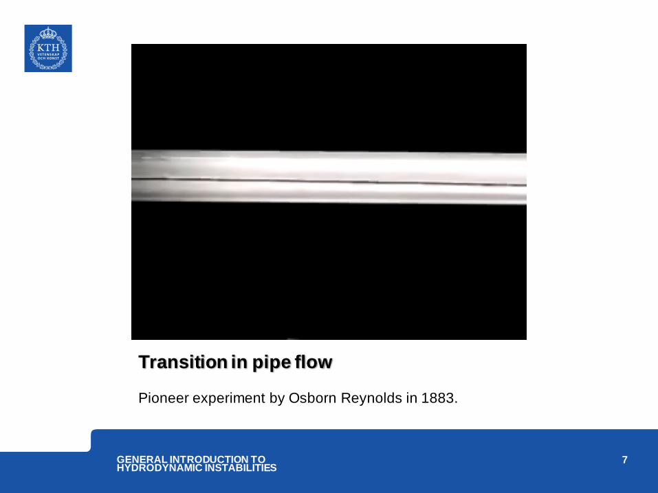
Transition in pipe flow
Pioneer experiment by Osborn Reynolds in 1883.

8 GENERAL INTRODUCTION TO HYDRODYNAMIC INSTABILITIES
Smoke from a cigarette.
Three different flow regimes can easily be identified :
laminar, transition and turbulence.
9 GENERAL INTRODUCTION TO HYDRODYNAMIC INSTABILITIES
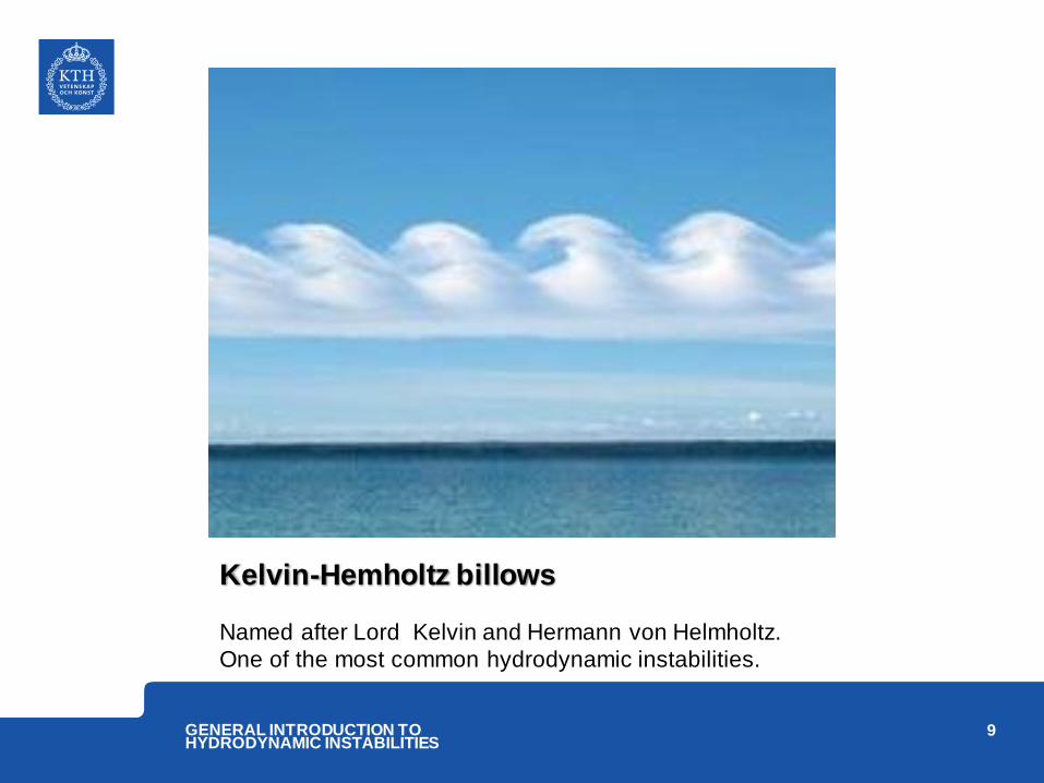
Kelvin-Hemholtz billows
Named after Lord Kelvin and Hermann von Helmholtz.
One of the most common hydrodynamic instabilities.
10 GENERAL INTRODUCTION TO HYDRODYNAMIC INSTABILITIES
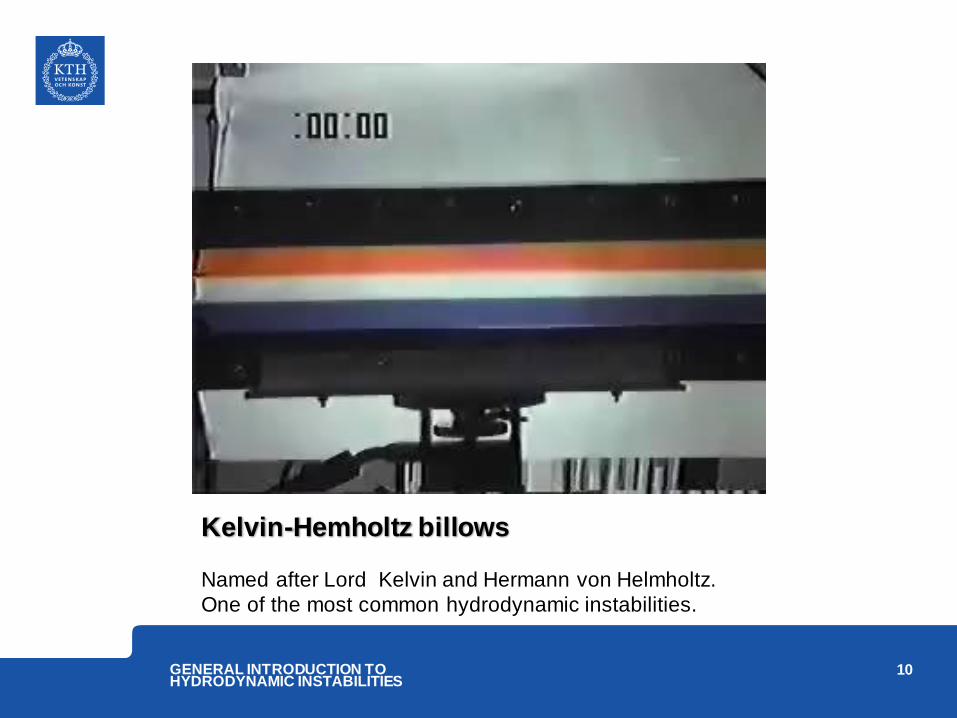
Kelvin-Hemholtz billows
Named after Lord Kelvin and Hermann von Helmholtz.
One of the most common hydrodynamic instabilities.
11 GENERAL INTRODUCTION TO HYDRODYNAMIC INSTABILITIES
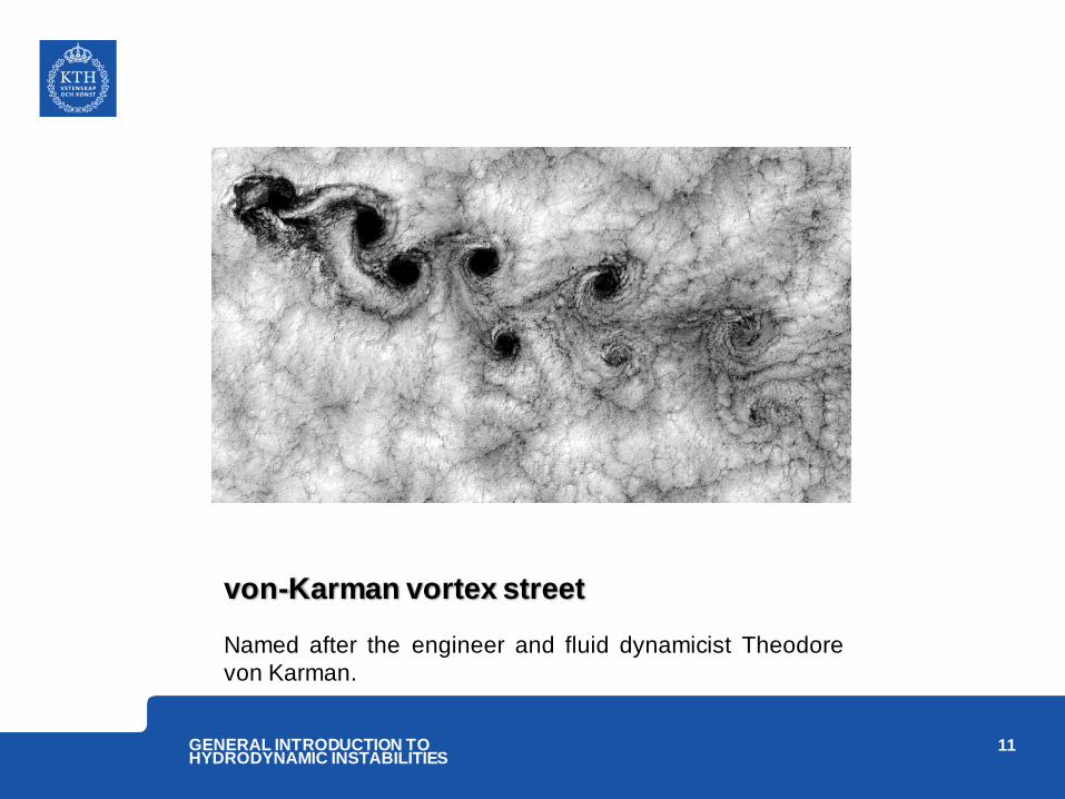
von-Karman vortex street
Named after the engineer and fluid dynamicist Theodore
von Karman.
12 GENERAL INTRODUCTION TO HYDRODYNAMIC INSTABILITIES
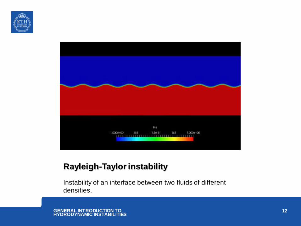
Rayleigh-Taylor instability
Instability of an interface between two fluids of different
densities.
13 GENERAL INTRODUCTION TO HYDRODYNAMIC INSTABILITIES
How do we study them?
Some definitions, mathematical formulation and a simple
example.
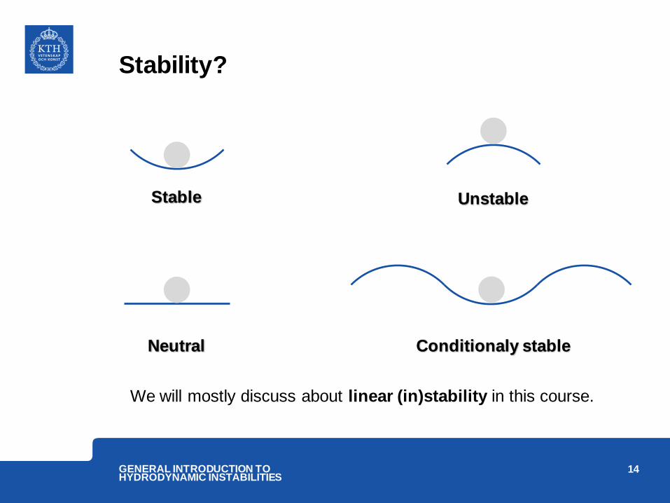
Stability?
14 GENERAL INTRODUCTION TO HYDRODYNAMIC INSTABILITIES
Stable Unstable
Neutral Conditionaly stable
We will mostly discuss about linear (in)stability in this course.
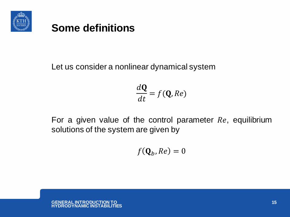
Some definitions
Let us consider a nonlinear dynamical system
𝑑𝐐
𝑑𝑡= 𝑓(𝐐, 𝑅𝑒)
For a given value of the control parameter 𝑅𝑒, equilibrium
solutions of the system are given by
𝑓 𝐐𝑏 , 𝑅𝑒 = 0
15 GENERAL INTRODUCTION TO HYDRODYNAMIC INSTABILITIES
Some definitions
16 GENERAL INTRODUCTION TO HYDRODYNAMIC INSTABILITIES
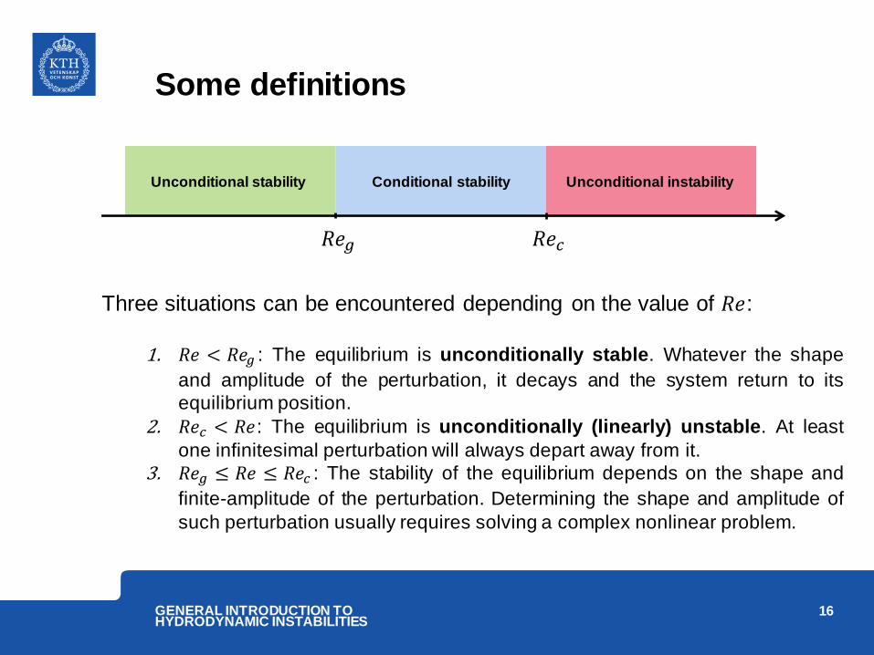
Unconditional stability Conditional stability Unconditional instability
𝑅𝑒𝑔 𝑅𝑒𝑐
Three situations can be encountered depending on the value of 𝑅𝑒:
1. 𝑅𝑒 < 𝑅𝑒𝑔 : The equilibrium is unconditionally stable. Whatever the shape
and amplitude of the perturbation, it decays and the system return to its
equilibrium position.
2. 𝑅𝑒𝑐 < 𝑅𝑒: The equilibrium is unconditionally (linearly) unstable. At least
one infinitesimal perturbation will always depart away from it.
3. 𝑅𝑒𝑔 ≤ 𝑅𝑒 ≤ 𝑅𝑒𝑐 : The stability of the equilibrium depends on the shape and
finite-amplitude of the perturbation. Determining the shape and amplitude of
such perturbation usually requires solving a complex nonlinear problem.
Mathematical formulation of the problem
• The first part of this course concerns linear stability
analysis, that is the determination of the unconditional
linear instability threshold 𝑅𝑒𝑐.
• The dynamics of an infinitesimal perturbation 𝐪 can be
studied by linearizing the system in the vicinity of the
equilibrium 𝐐𝑏
𝑑𝐪
𝑑𝑡= 𝐉𝐪
with 𝐉 the Jacobian matrix of the system evaluated at 𝐐𝑏.
17 GENERAL INTRODUCTION TO HYDRODYNAMIC INSTABILITIES
Mathematical formulation of the problem
The 𝑖𝑗-th entry of the Jacobian matrix evaluated in the vicinity
of 𝐐𝑏 is given by
𝐽𝑖𝑗 =𝜕𝑓𝑖
𝜕𝑄𝑗 𝐐𝑏
18 GENERAL INTRODUCTION TO HYDRODYNAMIC INSTABILITIES
Mathematical formulation of the problem
• This linear dynamical system is autonomous in time. Its
solutions can be sought in the form of normal modes
𝐪 𝑡 = 𝐪 𝑒𝜆𝑡 + 𝑐. 𝑐
with 𝜆 = 𝜎 + 𝑖𝜔.
• Injecting this form for 𝐪 𝑡 into our linear system yields the
following eigenvalue problem
𝜆𝐪 = 𝐉𝐪
19 GENERAL INTRODUCTION TO HYDRODYNAMIC INSTABILITIES
Mathematical formulation of the problem
The linear (in)stability of the equilibrium 𝐐𝑏 then depends on
the value of the growth rate 𝜎 = ℜ(𝜆) of the leading
eigenvalue :
1. If 𝜎 < 0, the system is linearly stable (𝑅𝑒 < 𝑅𝑒𝑐).
2. If 𝜎 > 0, the system is linearly unstable (𝑅𝑒 > 𝑅𝑒𝑐).
3. If 𝜎 = 0, the system is neutrally stable (𝑅𝑒 = 𝑅𝑒𝑐).
20 GENERAL INTRODUCTION TO HYDRODYNAMIC INSTABILITIES
Mathematical formulation of the problem
The value of 𝜔 = ℑ(𝜆) characterizes the oscillatory nature of
the perturbation :
1. If 𝜔 ≠ 0, the perturbation oscillates in time.
2. If 𝜔 = 0, the perturbation has a monotonic behavior.
21 GENERAL INTRODUCTION TO HYDRODYNAMIC INSTABILITIES
Exercise
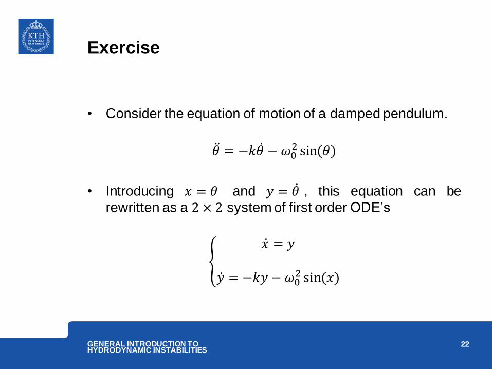
• Consider the equation of motion of a damped pendulum.
𝜃 = −𝑘𝜃 − 𝜔02 sin(𝜃)
• Introducing 𝑥 = 𝜃 and 𝑦 = 𝜃 , this equation can be
rewritten as a 2 × 2 system of first order ODE’s
𝑥 = 𝑦
𝑦 = −𝑘𝑦 − 𝜔02 sin(𝑥)
22 GENERAL INTRODUCTION TO HYDRODYNAMIC INSTABILITIES
Exercise
1. Compute the two equilibrium solutions of this system.
2. Derive the linear equations governing the dynamics of an
infinitesimal perturbation.
3. Study the linear stability of
a) the first equilibrium. Is it linearly stable or unstable?
b) the second one. Is it linearly stable or unstable?
23 GENERAL INTRODUCTION TO HYDRODYNAMIC INSTABILITIES

24 GENERAL INTRODUCTION TO HYDRODYNAMIC INSTABILITIES
Local hydrodynamic stability analysis
Navier-Stokes, Reynolds-Orr and Orr-Sommerfeld-Squire
equations

Navier-Stokes equations
• The dynamics of an incompressible flow of Newtonian fluid
are governed by
𝜕𝐔
𝜕𝑡= − 𝐔 ∙ 𝛻 𝐔 − 𝛻𝑃 +
1
𝑅𝑒𝛻2𝐔
𝛻 ∙ 𝐔 = 0
25 GENERAL INTRODUCTION TO HYDRODYNAMIC INSTABILITIES

Navier-Stokes equations
• It is a system of nonlinear partial differential equations
(PDE’s). The variables depend on both time and space.
• In the rest of this course, we will assume that the
equilibrium solution (or base flow) 𝐐𝑏 = (𝐔𝑏, 𝑃𝑏)𝑇 is given.
26 GENERAL INTRODUCTION TO HYDRODYNAMIC INSTABILITIES

Reynolds-Orr equation
• Assume a velocity field of the form
𝐔 = 𝐔 + 𝐮
27 GENERAL INTRODUCTION TO HYDRODYNAMIC INSTABILITIES

Reynolds-Orr equation
• Plugging it into the Navier-Stokes equations, the
governing equations for the fluctuation 𝐮 read
𝛻 ∙ 𝐮 = 0
𝜕𝐮
𝜕𝑡= − 𝐮 ∙ 𝛻 𝐔 − 𝐔 ∙ 𝛻 𝐮 − 𝛻𝑝 +
1
𝑅𝑒𝛻2𝐮 − 𝐮 ∙ 𝛻 𝐮
28 GENERAL INTRODUCTION TO HYDRODYNAMIC INSTABILITIES
Linear terms Nonlinear term

Reynolds-Orr equation
• Multiplying from the left by 𝐮 gives an evolution equation for
the local kinetic energy
1
2
𝜕
𝜕𝑡𝐮 ∙ 𝐮 = −𝐮 ∙ 𝐮 ∙ 𝛻 𝐔 − 𝐮 ∙ 𝐔 ∙ 𝛻 𝐮 + 𝐮 ∙
1
𝑅𝑒𝛻2𝐮
−𝐮 ∙ 𝛻𝑝 − 𝐮 ∙ 𝐮 ∙ 𝛻 𝐮
29 GENERAL INTRODUCTION TO HYDRODYNAMIC INSTABILITIES
Reynolds-Orr equation
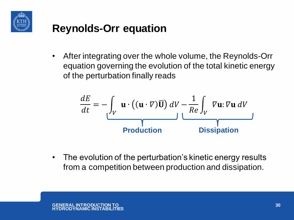
• After integrating over the whole volume, the Reynolds-Orr
equation governing the evolution of the total kinetic energy
of the perturbation finally reads
𝑑𝐸
𝑑𝑡= − 𝐮 ∙ 𝐮 ∙ 𝛻 𝐔 𝑑𝑉
𝑉−
1
𝑅𝑒 𝛻𝐮:𝛻𝐮 𝑑𝑉𝑉
• The evolution of the perturbation’s kinetic energy results
from a competition between production and dissipation.
30 GENERAL INTRODUCTION TO HYDRODYNAMIC INSTABILITIES
Production Dissipation
Reynolds-Orr equation
• These two terms only involve linear mechanisms whether
or not we initially considered the nonlinear term in the
momentum equation.
• The non-linear term is energy-conserving. It only scatters
the energy along the different velocity components and
length scales.
31 GENERAL INTRODUCTION TO HYDRODYNAMIC INSTABILITIES

Reynolds-Orr equation
• In the case of the Navier-Stokes equations, investigating
the dynamics of infinitesimal perturbation allows one to:
1. Identify the critical Reynolds number beyond which
the steady equilibrium flow is unconditionally unstable.
(Linear stability analysis)
2. Highlight the underlying physical mechanisms through
which any kind of perturbation (linear or nonlinear)
relies to grow over time. (Reynolds-Orr equation)
32 GENERAL INTRODUCTION TO HYDRODYNAMIC INSTABILITIES

Parallel flow assumption
• For the sake of simplicity, in the rest of the course we will
assume a base flow of the form
𝐔𝑏 = 𝑈 𝑦 , 0,0
• The base flow only depends on the cross-stream
coordinate. We neglect the streamwise evolution of the
flow.
33 GENERAL INTRODUCTION TO HYDRODYNAMIC INSTABILITIES
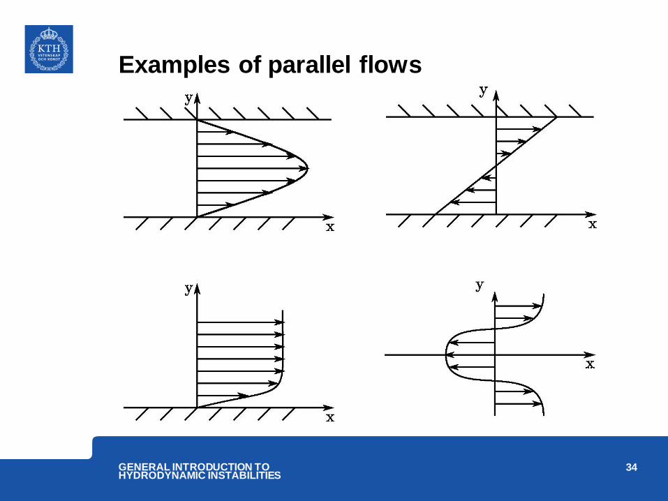
Examples of parallel flows
34 GENERAL INTRODUCTION TO HYDRODYNAMIC INSTABILITIES
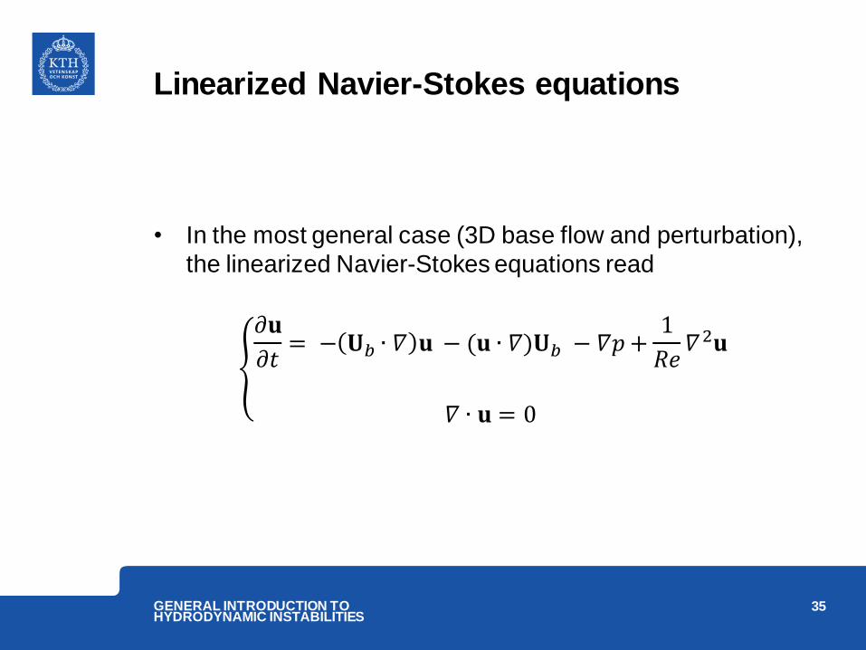
Linearized Navier-Stokes equations
• In the most general case (3D base flow and perturbation),
the linearized Navier-Stokes equations read
𝜕𝐮
𝜕𝑡= − 𝐔𝑏 ∙ 𝛻 𝐮 − (𝐮 ∙ 𝛻)𝐔𝑏 − 𝛻𝑝 +
1
𝑅𝑒𝛻2𝐮
𝛻 ∙ 𝐮 = 0
35 GENERAL INTRODUCTION TO HYDRODYNAMIC INSTABILITIES

Linearized Navier-Stokes equations
• Based on the parallel flow assumption used for 𝐔𝑏, these
equations simplify to
𝜕𝑢
𝜕𝑡= −𝑈𝑏
𝜕𝑢
𝜕𝑥− 𝑈𝑏
′𝑣 −𝜕𝑝
𝜕𝑥+
1
𝑅𝑒𝛻2𝑢
𝜕𝑣
𝜕𝑡= −𝑈𝑏
𝜕𝑣
𝜕𝑥 −
𝜕𝑝
𝜕𝑦+
1
𝑅𝑒𝛻2𝑣
𝜕𝑤
𝜕𝑡= −𝑈𝑏
𝜕𝑤
𝜕𝑥 −
𝜕𝑝
𝜕𝑧+
1
𝑅𝑒𝛻2𝑤
𝜕𝑢
𝜕𝑥+
𝜕𝑣
𝜕𝑦+
𝜕𝑤
𝜕𝑧= 0
36 GENERAL INTRODUCTION TO HYDRODYNAMIC INSTABILITIES

Orr-Sommerfeld equation
• Taking the divergence of the momentum equations gives
𝛻²𝑝 = −2𝑈𝑏′ 𝜕𝑣
𝜕𝑥
• One can now eliminate the pressure in the 𝑣-equation
𝜕
𝜕𝑡+ 𝑈𝑏
𝜕
𝜕𝑥𝛻² − 𝑈𝑏
′′ 𝜕
𝜕𝑥−
1
𝑅𝑒𝛻4 𝑣 = 0
• This is the Orr-Sommerfeld equation. It governs the
dynamics of the wall-normal velocity component of the
perturbation.
37 GENERAL INTRODUCTION TO HYDRODYNAMIC INSTABILITIES
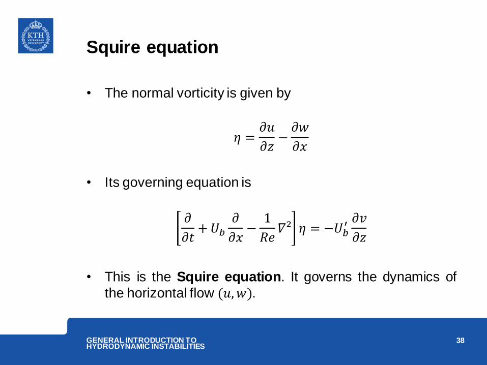
Squire equation
• The normal vorticity is given by
𝜂 =𝜕𝑢
𝜕𝑧−
𝜕𝑤
𝜕𝑥
• Its governing equation is
𝜕
𝜕𝑡+ 𝑈𝑏
𝜕
𝜕𝑥−
1
𝑅𝑒𝛻² 𝜂 = −𝑈𝑏
′ 𝜕𝑣
𝜕𝑧
• This is the Squire equation. It governs the dynamics of
the horizontal flow (𝑢, 𝑤).
38 GENERAL INTRODUCTION TO HYDRODYNAMIC INSTABILITIES
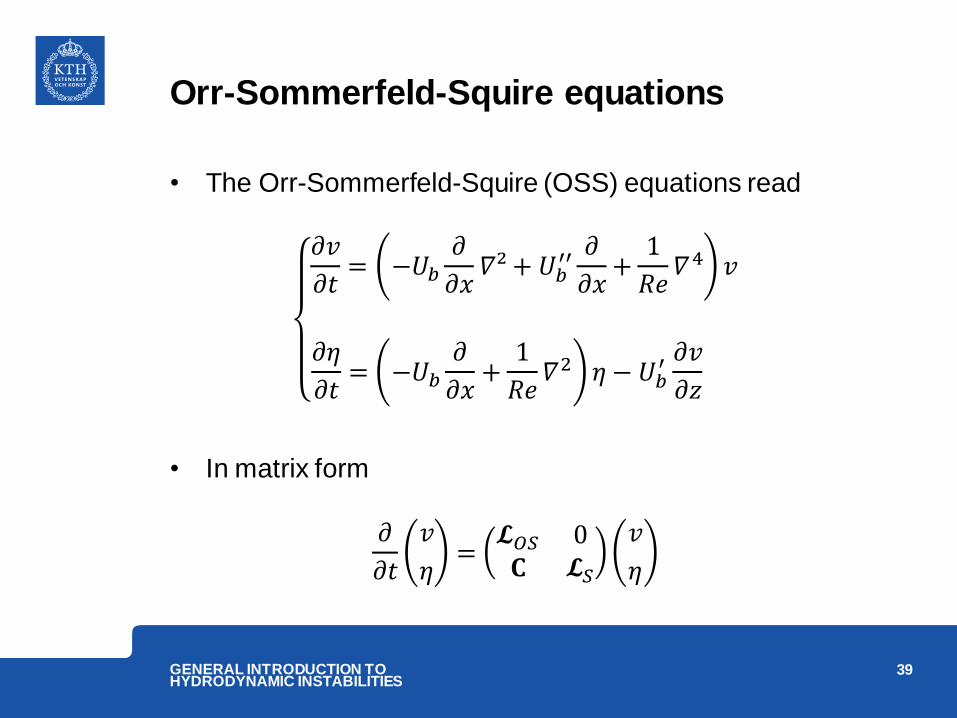
Orr-Sommerfeld-Squire equations
• The Orr-Sommerfeld-Squire (OSS) equations read
𝜕𝑣
𝜕𝑡= −𝑈𝑏
𝜕
𝜕𝑥𝛻² + 𝑈𝑏
′′ 𝜕
𝜕𝑥+
1
𝑅𝑒𝛻4 𝑣
𝜕𝜂
𝜕𝑡= −𝑈𝑏
𝜕
𝜕𝑥+
1
𝑅𝑒𝛻2 𝜂 − 𝑈𝑏
′ 𝜕𝑣
𝜕𝑧
• In matrix form
𝜕
𝜕𝑡
𝑣
𝜂=
𝓛𝑂𝑆 0𝐂 𝓛𝑆
𝑣
𝜂
39 GENERAL INTRODUCTION TO HYDRODYNAMIC INSTABILITIES

Orr-Sommerfeld-Squire equations
• The dynamics of the cross-stream velocity 𝑣 are
decoupled from the dynamics of the normal vorticity 𝜂.
• The linear stability of the Squire equation is dictated by the
linear stability of the Orr-Sommerfeld one.
• As a consequence, to determine the asymptotic time-
evolution (𝑡 → ∞ ) of an infinitesimal perturbation, it is
sufficient to consider the Orr-Sommerfeld equation only.
40 GENERAL INTRODUCTION TO HYDRODYNAMIC INSTABILITIES
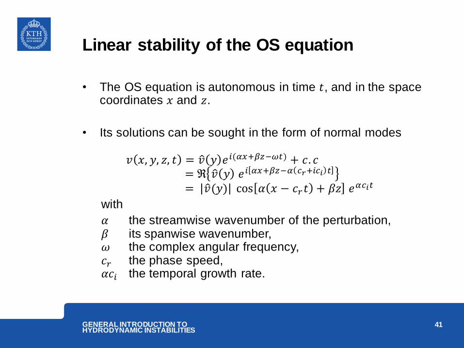
Linear stability of the OS equation
• The OS equation is autonomous in time 𝑡, and in the space coordinates 𝑥 and 𝑧.
• Its solutions can be sought in the form of normal modes
𝑣 𝑥, 𝑦, 𝑧, 𝑡 = 𝑣 𝑦 𝑒𝑖(𝛼𝑥+𝛽𝑧−𝜔𝑡) + 𝑐. 𝑐 = ℜ 𝑣 𝑦 𝑒𝑖 𝛼𝑥+𝛽𝑧−𝛼 𝑐𝑟+𝑖𝑐𝑖 𝑡
= 𝑣 (𝑦) cos 𝛼 𝑥 − 𝑐𝑟𝑡 + 𝛽𝑧 𝑒𝛼𝑐𝑖𝑡
with
𝛼 the streamwise wavenumber of the perturbation, 𝛽 its spanwise wavenumber, 𝜔 the complex angular frequency, 𝑐𝑟 the phase speed, 𝛼𝑐𝑖 the temporal growth rate.
41 GENERAL INTRODUCTION TO HYDRODYNAMIC INSTABILITIES
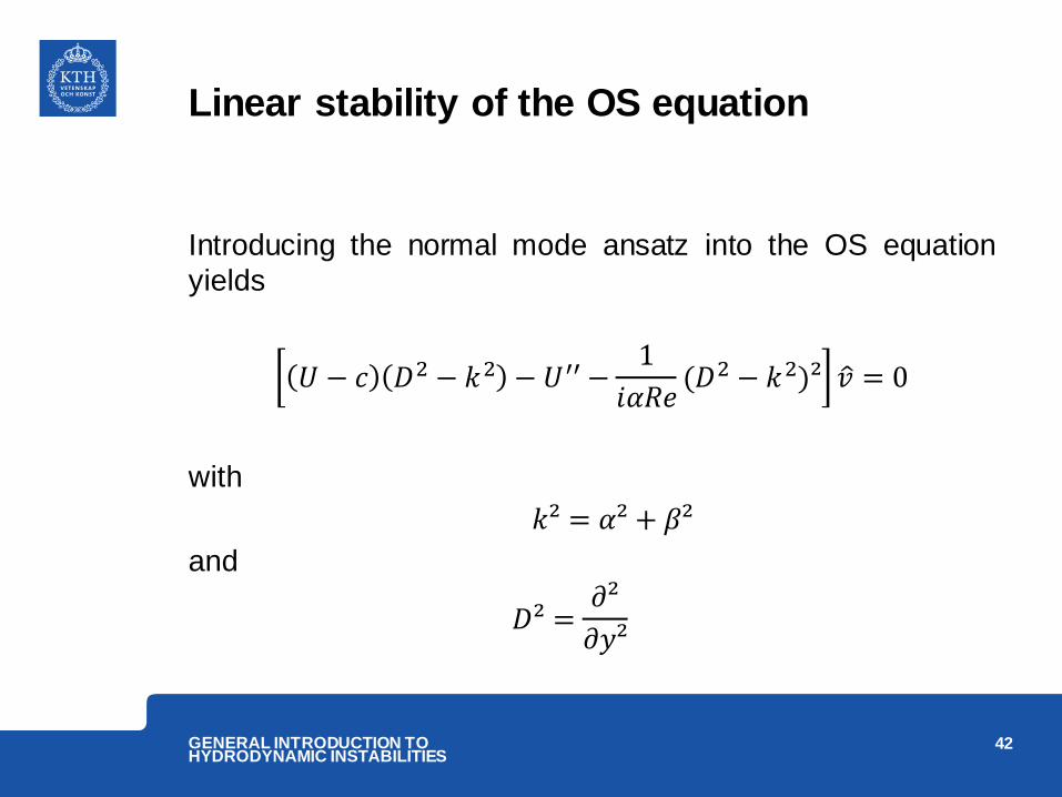
Linear stability of the OS equation
Introducing the normal mode ansatz into the OS equation
yields
𝑈 − 𝑐 𝐷2 − 𝑘2 − 𝑈′′ −1
𝑖𝛼𝑅𝑒(𝐷2 − 𝑘2)² 𝑣 = 0
with
𝑘² = 𝛼² + 𝛽²
and
𝐷² =𝜕²
𝜕𝑦²
42 GENERAL INTRODUCTION TO HYDRODYNAMIC INSTABILITIES
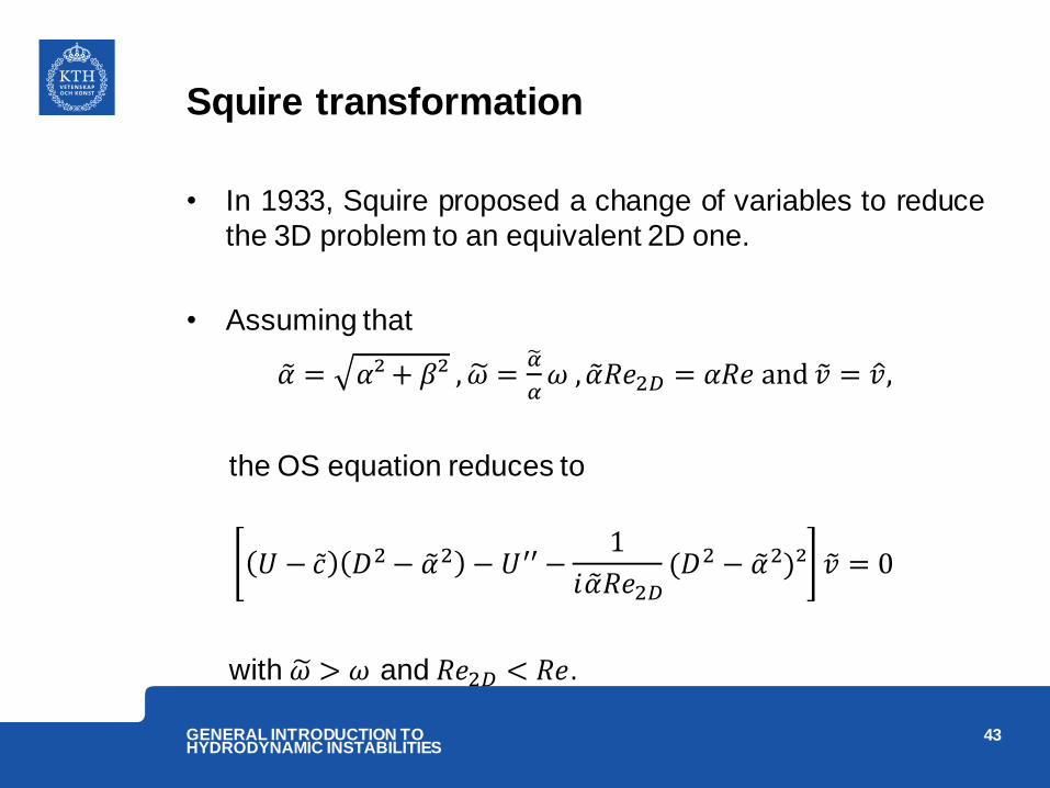
Squire transformation
• In 1933, Squire proposed a change of variables to reduce
the 3D problem to an equivalent 2D one.
• Assuming that
𝛼 = 𝛼² + 𝛽² , 𝜔 =𝛼
𝛼𝜔 ,𝛼 𝑅𝑒2𝐷 = 𝛼𝑅𝑒 and 𝑣 = 𝑣 ,
the OS equation reduces to
𝑈 − 𝑐 𝐷2 − 𝛼 2 − 𝑈′′ −1
𝑖𝛼 𝑅𝑒2𝐷(𝐷2 − 𝛼 2)² 𝑣 = 0
with 𝜔 > 𝜔 and 𝑅𝑒2𝐷 < 𝑅𝑒.
43 GENERAL INTRODUCTION TO HYDRODYNAMIC INSTABILITIES

Squire theorem (1933)
Theorem: For any three-dimensional unstable mode (𝛼, 𝛽, 𝜔) of temporal growth rate 𝜔𝑖 there is an associated two-
dimensional mode (𝛼 , 𝜔 ) of temporal growth rate
𝜔 𝑖 = 𝛼² + 𝛽²𝜔𝑖
𝛼
which is more unstable since 𝜔 𝑖 > 𝜔𝑖. Therefore, when the
problem is to determine an instability condition, it is sufficient
to consider only two-dimensional perturbations.
44 GENERAL INTRODUCTION TO HYDRODYNAMIC INSTABILITIES

45 GENERAL INTRODUCTION TO HYDRODYNAMIC INSTABILITIES
Summary
Summary
• Hydrodynamic instabilities are ubiquitous in nature.
• Though the Navier-Stokes equations are nonlinear PDE’s,
the kinetic energy transfer from the base flow to the
perturbation is governed by a linear equation (Reynolds-
Orr equation).
• Hence, as a first step toward our understanding of
transition to turbulence, investigating the dynamics of
infinitesimally small perturbations governed by the
linearized Navier-Stokes equations can prove useful.
46 GENERAL INTRODUCTION TO HYDRODYNAMIC INSTABILITIES
Summary
• Investigating the linear stability of a given system is a four-
step procedure:
1. Compute an equilibrium solution 𝐐b of the original
nonlinear system.
2. Linearize the equations in the vicinity of 𝐐𝑏.
3. Use the normal mode ansatz to formulate the problem
as an eigenvalue problem.
4. Solve the eigenvalue problem.
• The linearly stable or unstable nature of 𝐐𝑏 is governed
by the eigenspectrum of the Jacobian matrix.
47 GENERAL INTRODUCTION TO HYDRODYNAMIC INSTABILITIES
Summary
• For the Navier-Stokes equations, using the parallel flow assumption greatly reduces the complexity of the perturbation’s governing equations.
• Making use of the Orr-Sommerfeld-Squire equations decreases the dimension of the problem from ℝ4𝑛 to ℝ2𝑛 .
• The linear (in)stability of the flow is solely governed by the Orr-Sommerfeld equation, thus further reducing the dimension of the problem down to ℝ𝑛.
• Thanks to the Squire theorem, it is sufficient to investigate the linear stability of two-dimensional perturbations to determine the instability condition.
48 GENERAL INTRODUCTION TO HYDRODYNAMIC INSTABILITIES
Inviscid instability of parallel flows Rayleigh equation, Rayleigh, Fjørtotf and Howard theorems and the vortex sheet instability
49 GENERAL INTRODUCTION TO HYDRODYNAMIC INSTABILITIES

Rayleigh equation
• The linear (in)stability of a viscous parallel flow is
governed by the Orr-Sommerfeld equation
𝑈 − 𝑐 𝐷2 − 𝛼2 − 𝑈′′ −1
𝑖𝛼𝑅𝑒(𝐷2 − 𝛼2)² 𝑣 = 0
• In the inviscid limit (𝑅𝑒 → ∞), it reduces to the Rayleigh
equation
𝑈 − 𝑐 𝐷2 − 𝛼2 − 𝑈′′ 𝑣 = 0
GENERAL INTRODUCTION TO HYDRODYNAMIC INSTABILITIES
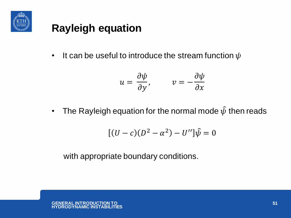
Rayleigh equation
• It can be useful to introduce the stream function 𝜓
𝑢 = 𝜕𝜓
𝜕𝑦, 𝑣 = −
𝜕𝜓
𝜕𝑥
• The Rayleigh equation for the normal mode 𝜓 then reads
𝑈 − 𝑐 𝐷2 − 𝛼2 − 𝑈′′ 𝜓 = 0
with appropriate boundary conditions.
51 GENERAL INTRODUCTION TO HYDRODYNAMIC INSTABILITIES
Rayleigh inflection point theorem
Theorem: The existence of an inflection point in the velocity
profile of a parallel flow is a necessary (but not sufficient)
condition for linear instability.
52 GENERAL INTRODUCTION TO HYDRODYNAMIC INSTABILITIES
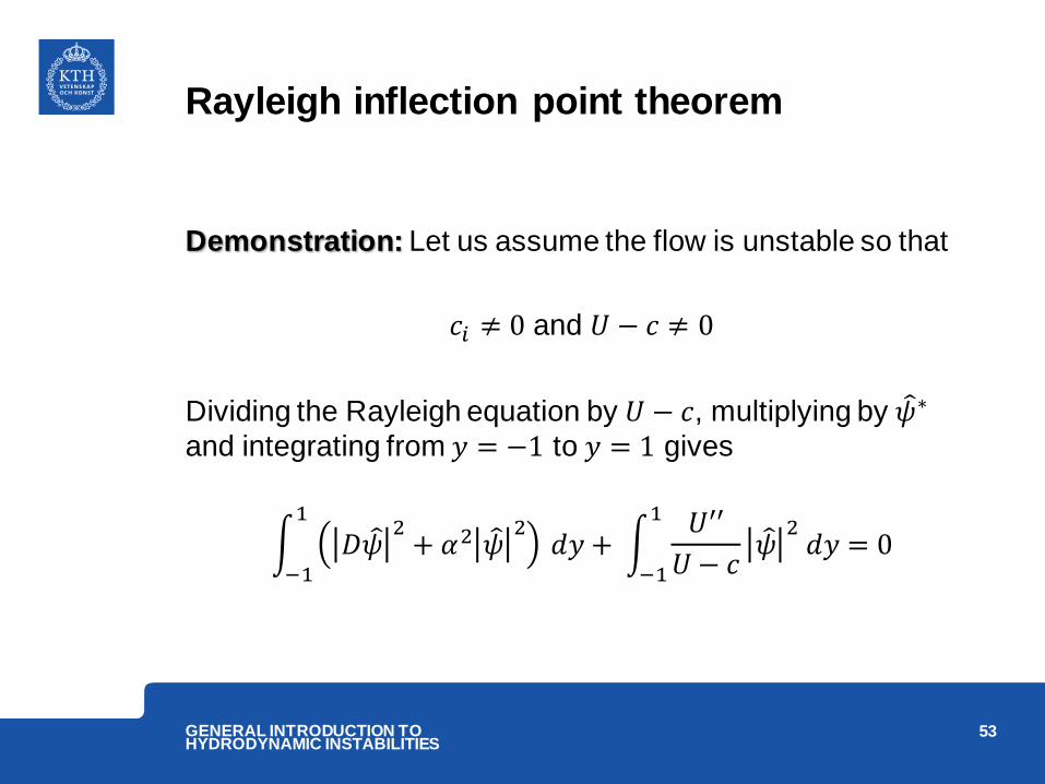
Rayleigh inflection point theorem
Demonstration: Let us assume the flow is unstable so that
𝑐𝑖 ≠ 0 and 𝑈 − 𝑐 ≠ 0
Dividing the Rayleigh equation by 𝑈 − 𝑐, multiplying by 𝜓 ∗
and integrating from 𝑦 = −1 to 𝑦 = 1 gives
𝐷𝜓 2
+ 𝛼2 𝜓 2
1
−1 𝑑𝑦 +
𝑈′′
𝑈 − 𝑐𝜓
2 𝑑𝑦
1
−1= 0
53 GENERAL INTRODUCTION TO HYDRODYNAMIC INSTABILITIES

Rayleigh inflection point theorem
Let us consider only the imaginary part of this integral
ℑ 𝑈′′
𝑈 − 𝑐𝜓
2 𝑑𝑦
1
−1=
𝑐𝑖𝑈′′
𝑈 − 𝑐 2 𝜓 2 𝑑𝑦
1
−1= 0
By assumption, we have 𝑐𝑖 ≠ 0 and this integral must vanish.
As a consquence 𝑈′′(𝑦) must change sign, i.e., the velocity
profile must have an inflection point.
54 GENERAL INTRODUCTION TO HYDRODYNAMIC INSTABILITIES

Rayleigh inflection point theorem
55 GENERAL INTRODUCTION TO HYDRODYNAMIC INSTABILITIES

Rayleigh inflection point theorem
• According to the Rayleigh theorem :
o Velocity profile (a) is stable (in the inviscid limit).
o Vecolity profiles (b) and (c) can potentially be
unstable.
• One important conclusion of this theorem is that, if the
effect of viscosity on the pertubation is neglected,
both the Poiseuille flow and the Blasius boundary layer
flow are stable (see profile (a) )..
56 GENERAL INTRODUCTION TO HYDRODYNAMIC INSTABILITIES
Fjørtoft theorem
Theorem: For a monotonic velocity profile, a necessary (but
still not sufficient) condition for instability is that the inflection
point corresponds to a vorticity maximum.
57 GENERAL INTRODUCTION TO HYDRODYNAMIC INSTABILITIES
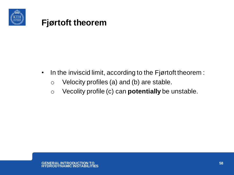
Fjørtoft theorem
• In the inviscid limit, according to the Fjørtoft theorem :
o Velocity profiles (a) and (b) are stable.
o Vecolity profile (c) can potentially be unstable.
58 GENERAL INTRODUCTION TO HYDRODYNAMIC INSTABILITIES

Application to KH-instability
59 GENERAL INTRODUCTION TO HYDRODYNAMIC INSTABILITIES
‘’Bernoulli effect’’-like explanation of the Kelvin-Helmholtz instability.
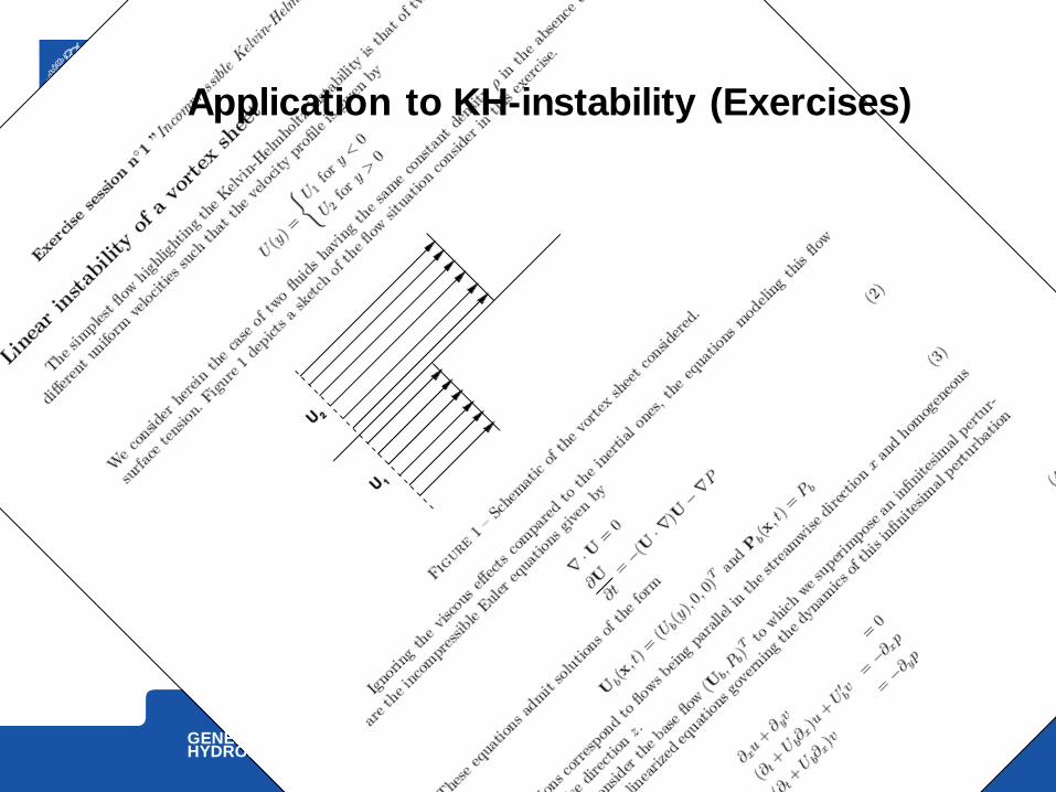
Application to KH-instability (Exercises)
60 GENERAL INTRODUCTION TO HYDRODYNAMIC INSTABILITIES

61 GENERAL INTRODUCTION TO HYDRODYNAMIC INSTABILITIES
Summary
Summary
• If we assume that the inertial effects are much larger than
the viscous ones (𝑅𝑒 → ∞), the Orr-Sommerfeld equation
reduces to the Rayleigh equation.
• Rayleigh theorem states that an inflection point in the
velocity profile is a necessary (but not sufficient) condition
for inviscid instability.
• Fjørtoft theorem states that this inflection point needs to
correspond to a maximum in the vorticity distribution. This
is however still just a necessary (but not sufficient)
condition for inviscid instability.
62 GENERAL INTRODUCTION TO HYDRODYNAMIC INSTABILITIES
Summary
• Ignoring all effects of viscous diffusion leads to an
unbounded growth rate at large wave numbers (small
wavelength).
• Despite this limitation, the vortex sheet problem enable a
relatively good understanding of the Kelvin-Helmholtz
instability process.
• More realistic models, as the broken line velocity profile,
avoids the divergence of the growth rate at large wave
numbers while retaining the invisicid approximation.
63 GENERAL INTRODUCTION TO HYDRODYNAMIC INSTABILITIES