general methods for monitoring convergence of iterative...

General Methods for Monitoring Convergence of Iterative Simulations

Stephen P. BROOKSand Andrew GELMAN

We generalize the method proposed by Gelman and Rubin (1992a) for monitoring the convergence of iterative simulations by comparing between and within variances of multiple chains, in order to obtain a family of tests for convergence. We review methods of inference from simulations in order to develop convergence-monitoring summaries that are relevant for the purposes for which the simulations are used. We recommend applying a battery of tests for mixing based on the comparison of inferences from individual sequences and from the mixture of sequences. Finally, we discuss multivariate analogues, for assessing convergence of several parameters simultaneously.

Key Words: Convergence diagnosis; Inference; Markov chain Monte Carlo.

1. INTRODUCTION AND BACKGROUND Markov chain Monte Carlo (MCMC) algorithms have made a significant impact on

the range of problems to which Bayesian analyses can be applied; see Gilks, Richardson, and Spiegelhalter (1996). The method involves simulating from a complex and generally multivariate target distribution, p ( Q ) , indirectly, by generating a Markov chain with the target density as its stationary density. Generally, we run m > 1 sequences of simulations, each of length n, (Q,, , Q32. . . . . Q J n ) ,for j = 1 , .. . .m. (In this notation, each QJt is a vector.) If m > 1, the m sequences are usually, but not always, simulated independently.

One might like to analytically compute or estimate a convergence rate and then take sufficient iterations for any particular desired accuracy but this is not possible in general (Tierney 1994). It is possible to find bounds on the rates of convergence for special classes of Markov chains (e.g., Rosenthal 1995), but in practice it is difficult to apply these results effectively in the context of MCMC.

In the absence of any general techniques for a priori prediction of run lengths, it is necessary to carry out some form of statistical analysis in order to assess convergence. These procedures, which are called convergence diagnostics, fall into two general cat- egories: those based solely on the output values (Q,t) of the simulation, and those that also use additional information about the target density; the methods described in this

Stephen P. Brooks is Lecturer. Department of Mathematics, University of Bristol, University Walk, Bristol, BS8 ITW, England (E-mail: [email protected]). Andrew Gelman is Associate Professor, Department of Statistics. Columbia University, New York, NY 10027.

0 1 9 9 8 American Statistical Association, Institute of Mathematical Statistics, and Interjiace Foundation of North America

Journal of Computational and Graphical Statistics, Volume 7, Number 4, Pages 434455

article are all of the first category. See Brooks and Roberts (in press) and Cowles and Carlin (1996) for reviews of commonly used techniques of convergence assessment.

Gelman and Rubin (1992a,b) pointed out that, in many problems, lack of convergence can be easily determined from multiple independent sequences but cannot be diagnosed using simulation output from any single sequence. They proposed a method using multiple replications of the chain to decide whether or not stationarity has been achieved within the second half of each of the sample paths. The idea behind this is an implicit assumption that convergence will have been achieved within the first half of the sample paths, and the validity of this assumption is essentially being tested by the diagnostic. This method's popularity may be largely due to its implementational simplicity and the fact that generic code is widely available to implement the method. In addition, even when this method is not formally used, something like it is often done implicitly or informally.

For example, Green, Roesch, Smith, and Strawderman (1994) wrote, in implementing a Gibbs sampler, "In the present study we used . . . one long chain. Experimentation with different starting values convinced us that the chain was converging and covering the entire posterior distribution." As is often the case in statistics, it generally useful to study the formal procedures that lie behind an informal method, in this case for monitoring the mixing of multiple sequences.

In this article, we generalize the method of Gelman and Rubin (1992a) by (1) adding graphical methods for tracking the approach to convergence; (2) generalizing the scale reduction factor to track measures of scale other than the variance; and (3) extending to multivariate summaries. Before presenting these extensions, we summarize the motivation underlying and the details of the original method.

Operationally, effective convergence of Markov chain simulation has been reached when inferences for quantities of interest do not depend on the starting point of the simulations. This suggests monitoring convergence by comparing inferences made from several independently sampled sequences with different starting points. Before considering methods of comparing inferences, we briefly discuss the standard method for constructing inferences under the assumption that convergence has been approximately reached. It is standard practice to discard observations within an initial transient phase. Most methods for inference are then based on the assumption that what remains can be treated as if the starting points had been drawn from the target distribution (for an exception, see Liu and Rubin in press).

Inference for random variables (e.g., posterior quantities in a Bayesian analysis), for which we use the notation y = y(Q) , is straightforward: a (1 - 0 ) central posterior interval for a scalar random variable $ under the target distribution is approximated by the 012 and 1-012 quantiles of the empirical simulation results, wit, from all sequences together (if m > 1) and discarding bum-in iterations. This is, of course, also the standard procedure for obtaining intervals from direct (noniterative) simulation, and is generally recommended no matter how convergence is monitored; for example, Gelman and Rubin (1992a) used an approximate Student-t posterior distribution to estimate convergence but

then recommend using the empirical intervals once approximate convergence has been reached. When additional information about the target distribution is used, inference can be made much more precise, as in the "Rao-Blackwellization" procedure of Gelfand and Smith (1990), which uses the analytic form of the conditional target distribution of $ given the rest of 8 (see also Tanner and Wong 1987). However, even these procedures are ultimately applied by averaging over the iterations of all the simulated sequences, after discarding burn-in.

This suggests that "convergence" can be quantified in terms of the properties of the empirical interval, as compared to the true 95% interval from the target distribution, which would be attained in the limit as n + co.

As background, we present the method of Gelman and Rubin (1992a) using our general perspective of comparison of inferences. The method presupposes that m chains have been simulated in parallel, each with different starting points which are overdispersed with respect to the target distribution. A number of methods have been proposed for generating initial values for MCMC samplers. Gelman and Rubin (1992a) proposed using a simple mode-finding algorithm to locate regions of high density and sampling from a mixture of t-distributions located at these modes to generate suitable starting values. An alternative approach was presented by Applegate, Kannan, and Polson (1990) who used the method of simulated annealing in this same context; see also Jennison (1993). Having obtained suitable starting points, the chains are then run for 2n iterations, of which the first n are discarded to avoid the burn-in period.

Given any individual sequence, and if approximate convergence has been reached, an assumption is made that inferences about any quantity of interest is made by computing the sample mean and variance from the simulated draws. Thus, the m chains yield m possible inferences; to answer the question of whether these inferences are similar enough to indicate approximate convergence, Gelman and Rubin (1992a) suggested comparing these to the inference made by mixing together the mn draws from all the sequences. Consider a scalar summary-that is, a random variable-$, that has mean p and variance a2under the target distribution, and suppose that we have some unbiased estimator for p. Letting $,t denote the tth of the n iterations of $ in chain j , we take jZ = $.., and calculate the between-sequence variance B l n , and the within-sequence variance W , defined by

Note that the ANOVA assumption of pooled within variances can be made here because, under convergence, the m within-chain variances will indeed be equal.

Having observed these estimates, we can estimate a2by a weighted average of B

and W ,

B / ( m n ) .+ 6:

which would be an unbiased estimate of the true variance o', if the starting points of the sequences were drawn from the target distribution, but overestimates a' if the starting distribution is appropriately overdispersed. (As we shall see in Section 2.1. if over-dispersion does not hold, 6: can be too low. which can lead to falsely diagnosing convergence.) Accounting for the sampling variability of the estimator yields a pooled

A

posterior variance estimate of = The comparison of pooled and within-chain inferences is expressed as a variance

ratio.

which is called the scale reduction factor, or SRF. (Strictly speaking. the term "scale reduction factor" applies to &: for convenience, we will mostly work with variance reduction factors in this article.) Because the denominator of R is not itself known, it must be estimated from the data: we can gain an overestimate of R by (under)estimating a' by W .Thus, we (0ver)estimate R by

which is called the potential scale reduction factor, or PSRF, and can be interpreted as a convergence diagnostic as follows. If 5 is large, this suggests that either estimate of the variance 8' can be further decreased by more simulations, or that further simulation will increase IT', since the simulated sequences have not yet made a full tour of the target distribution. Alternatively, if the PSRF is close to 1, we can conclude that each of the m sets of n simulated observations is close to the target distribution.

From our perspective of monitoring convergence based on the behavior of potential inferences, Gelman and Rubin's approach applies to all those situations where inferences are summarized by posterior means and variances, even if the posterior distributions are not themselves believed to be normally distributed. Other measures of convergence may be more appropriate if one is planning to use distributional summaries other than the first two moments.

One can refine the PSRF to account for sampling variability in the variance estimates. following the method of Fisher (1935) based on independent samples from the normal distribution. The key parameter for this adjustment is the estimated degrees of freedom, d, for a Student-t approximation to the posterior inference based upon the simulations. The degrees of freedom can be estimated by the method of moments: d % 2F/=r(F)').

Gelman and Rubin (1992a) incorrectly adopted the correction factor d / ( d- 2 ) . This represents the ratios of the variances of the td and the normal distributions. The use of

this incorrect factor has led to a number of problems, in that the corrected SRF (CSRF) can be infinite or even negative in the cases where convergence is so slow that d < 2. In order to correctly account for the sampling variability, the correction factor (d+3)/(d+ 1) should be used. The correct factor, (d + 3)/(d + I ) , removes the problems associated with that proposed in the original article.

A

We can motivate this correction factor as follows. Given an estimator $, with associated sampling variance s2 estimated on d degrees of freedom, the position is not the same as if the variance were known exactly. Our estimate of the variance is itself subject to variability and allowance for this is made by adopting the t-distribution rather than the normal. Thus, it is incorrect to assume that the information supplied by 6is l / s2 , as though the estimate were known to follow a normal distribution with this variance. Instead, we need to account for not only the estimate s2, but also the degrees of freedom upon which it is based. Thus, the correction factor (d + 3) / (d + 1 ) comes from the evaluation of Fisher's information for the td distribution, correcting our estimator p for the degrees of freedom on which it is based. see Fisher (1935).

Thus, we define

This correction is minor, because at convergence d tends to be large.

2. AN ITERATED GRAPHICAL APPROACH Gelman and Rubin (1992a) originally proposed running the chains for 2 n iterations

and basing the calculation of 2,upon the final n of these, for each parameter of interest. They suggest that if a,is close to 1 for each parameter, then the latter half-sequences

A

can be said to have converged. However, if R, is much greater than 1 for any parameter of interest, this suggests that one should either continue the simulation or assume that there is some facet of the model which is causing slow convergence.

A

The method of monitoring convergence by examining a ratio, R,,ignores some information in the simulations. In particular, at convergence, the following three conditions should hold:

1. The mixture-of-sequences variance, V, should stabilize as a function of n. (Before convergence, we expect 8: to decrease with n, only increasing if the sequences explore a new area of parameter space, which would imply that the original sequences were not overdispersed for the particular scalar summary being monitored.)

2. The within-sequence variance, W , should stabilize as a function of n. (Before convergence, we expect W to be less than V.)

3. As previously discussed, 2,should approach 1. Monitoring 2,alone considers only the third of these conditions.

An alternative, graphical approach to monitoring convergence is to divide the m sequences into batches of length b. We can then calculate V(k), W(k) , and Ec(lc)based upon the latter half of the observations of a sequence of length 2kb, for k = 1 , . . . ,n/b, for some suitably large n. Note that we still choose to discard the first half of each sample,

but argue that this choice is reasonable in terms of computational efficiency. If we discard a greater proportion of the samples, then this would be wasteful, since the diagnostic would be based upon only a small fraction of the samples available. However, if we choose to discard less than half of each sample, then the sample of observations used at each iteration would change too little, and the E value would remain high for too long, due to its continued dependence upon samples within the burn-in. Thus, the diagnostic would be wasteful in the sense that it would diagnose convergence later than necessary. Discarding half of the available sample at each iteration provides a compromise that attempts to maximize overall efficiency.

The iterative diagnostic procedure can be done either as observations are generated, or post-simulation as with the original method. In this way, we construct sequences that we can plot against k (or, equivalently 2kb) in order to monitor the chains as they converge. In order to choose a suitable value of b, we note that a small value of b increases computational expense, whereas a large value provides little extra information in terms of convergence monitoring. In practice, experience suggests that taking b zn/20 provides a reasonable output and minimizes computational overheads.

In addition to the plot of &(k) against k, another useful diagnostic is obtained by plotting the two scale factors, ~ ' / ~ ( k ) as a function of k together on the and ~ ' / ~ ( k ) , same plot. (We use the power so that the factors are on a more directly interpretable scale.) Approximate convergence is not attained until both lines stabilize (conditions 1 and 2), and they stabilize at the same value (condition 3). We illustrate with an example.

Grieve (1987) provided data that measure photocarcinogenicity or survival times for four groups of mice subjected to different treatments. The survival times are assumed to follow a Weibull distribution, so that the likelihood is given by n,(peP'zttf-l 1ct

exp(-ep'zatf). where t, denotes the failure or censure time of an individual, p > 0 is the shape parameter of the Weibull distribution, 3 is a vector of unknown parameters, the z, denote covariate vectors assigning each observation to one particular treatment group, and c, is an indicator variable such that c, = 1 if t , is uncensored and c, = 0 otherwise.

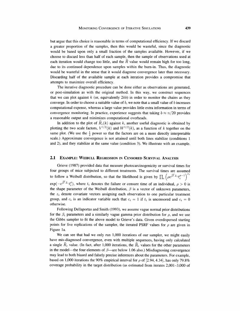
Following Dellaportas and Smith (1993), we assume vague normal prior distributions for the 3, parameters and a similarly vague gamma prior distribution for p, and we use the Gibbs sampler to fit the above model to Grieve's data. Given overdispersed starting points for five replications of the sampler, the iterated PSRF values for p are given in Figure la .

We can see that had we only run 1,000 iterations of our sampler, we might easily have mis-diagnosed convergence, even with multiple sequences, having only calculated a single E,value. (In fact, after 1,000 iterations, the 2,values for the other parameters in the model-the four elements of /I--are below 1.06 also.) Misdiagnosing convergence may lead to both biased and falsely precise inferences about the parameters. For example, based on 1,000 iterations the 90% empirical interval for p of [2.94,4.34], has only 79.8% coverage probability in the target distribution (as estimated from iterates 2,001-3,000 of

Iteration no

(b)

Iteration no Figure I . (a ) Iterative PSRF Plotfor p in the Weibull example (from m = 5 parallel sequences and with b = 50). After 1,000 or 1,200 iterations, the PSRF could misleadingly suggest that convergence has been obtained. (b ) Plots of ? ' I 2 (solid) and w112(dotted) for this example. Not until about 2,500 iterations are both lines stable and close to each other.

all five replications). However, Figure 1 only checks the third of the three conditions necessary for con-

vergence. We would not be misled in this way if we looked at the plots of v1I2and w'/*,as displayed in Figure lb. In the crucial period from iterations 800 to 1,300, when E,goes rapidly below 1.1 (misleadingly suggesting convergence), neither V nor W has stabilized-they both appear to be increasing in this region. This suggests that neither of the first two convergence conditions have yet been satisfied. It is not until beyond around 2,500 iterations that both plots begin to level out at a constant value, satisfying all three conditions above for convergence. The behavior of V and W as a function of time suggests that the starting points were not sufficiently overdispersed. In this case, all five replications have explored only a single portion of the parameter space. At iteration 1,300, one of the chains "discovers" the remaining portion, which is subsequently explored by the others by iteration 2,500. By continuing the chain beyond 5,000 iterations, we can be reasonably certain that convergence was achieved after about 2,500 iterations.

Thus, the iterated, graphical method presents a qualitative element to the diagnostic, which gives the user a better "feel" for what is really happening with the chains, in a similar way to the cusum plot of Yu (1995). However, given a large number of parameters, the univariate graphical approach soon becomes impractical, which suggests that a numerical approach for checking the stability of V and W would be desirable.

3. GENERAL UNIVARIATE COMPARISONS A limitation of the original convergence diagnostic is the assumption of normality

of the marginal distribution of each scalar quantity, v.Normality is assumed explicitly when using the correction factor (d +3) / (d+ 1 ) and, more importantly, implicitly when comparing the mixing of sequences by monitoring means and variances. The assumption of normality can be made more reasonable by appropriate transformations such as logs and logits, as Gelman and Rubin (1992a) suggested, but it is still unappealing, especially considering that MCMC methods are often used for highly non-normal, and even mul- timodal, densities. Here, we define a family of potential scale reduction factors, each of which has an interpretation as a measure of mixing and with the property that 2 -+ 1 as convergence is approached, but which avoid the assumption of normality.

An alternative interpretation of the 2 diagnostic is as a (squared) ratio of interval lengths, rather than as a variance ratio. This interpretation leads to an alternative imple- mentation that can be used whenever sequences are long enough. Suppose we seek a 100(1- a)% interval for some parameter, $. Then we construct 6,based upon the final n of the 2 n iterations, as follows.

1. From each individual chain, take the empirical 100(1- a)% interval; that is, the 1007% and the 100(1 - f ) % points of the n simulation draws. Thus, we form m within-sequence interval length estimates.

2. From the entire set of m n observations, gained from all chains, calculate the empirical 100(1- a)% interval, gaining a total-sequence interval length estimate.

3. Evaluate 6 defined as A length of total-sequence interval Rinterval = mean length of the within-sequence intervals '

This method is considerably simpler than the original method. It is very easy to A

implement and does not even require second moments, let alone normality. RinterValis still a PSRF, but based upon empirical interval lengths as a measure of information, rather than variance estimates. Like the normal-based diagnostic, &,,,,,l has the property of approaching 1 as the chains converge. Note that we do have the constraint that n be large enough to determine the empirical within-sequence intervals, but in practice, this does not generally seem to be a problem.

However, this is not the only possible interval-based approach. An alternative diagnostic can be defined based on coverage probability, as follows.

1 . From each individual chain, take the end-points of the empirical 100(1 - a)% interval to get a "within-chain" i~ terval estimate.

2. For each of the within-chain intervals, estimate the empirical coverage probability of that interval with reference to the combination of all m sequences combined; that is, calculate the proportion of observations from all m sequences combined, which lie within that interval.

3. Compute the average empirical coverage probability of the m intervals. At convergence, this will equal the nominal coverage probability, 1 - a .

Non interval-based alternatives are also possible. For example, if higher order mo-

ments can be assumed to exist, and are of interest, one can replace the numerator and denominator in (1.1) by an empirical estimate of the central sth order moments calculated from all sequences together and the mean sth order moment calculated from each individual sequence, respectively. Thus, we define

for any value of s which seems reasonable within the context of the problem at hand. A

Corresponding graphical displays plot the numerator and denominator of R,,t,,,,l, or R,, together for sequences of length 2kb, k = 1 , . . . , n l b as described in Section 2. These plots may then clarify the reasons for nonconvergence.

The second-order measure, &, is clearly similar to R defined in Section 1.2; some algebraic manipulation yields

- ( m - 1)n8: n - 1R2 = -+ ---m n - 1 W m n - 1

(compare to (1.1)), and for moderately large n (so that % I),

5- For example, if m = 5 and $ = 1.2, then R = 1.24 and R2 = 1.16. In defining these alternative measures, we ignore the correction factor (d+3)/(d+ 1).

This is appealing because we no longer assume normality but, of course, also means that we ignore some of the sampling variability in our estimate. In general, this correction factor has negligible effect upon the decision as to when convergence is achieved since first, if 2, < 1.1, say, then we should have enough observations so that its sampling variability is negligible; and second, in those cases where the effect is non-negligible, the chains are far from convergence and the ratio 2 = F / w will be large anyway. However, if this is a concern, the correction factor (d + 3)/(d + 1) can be computed (using the implicit normal model) and multiplied into the alternative measures; this is similar to the semi-parametric bootstrap idea of using a model to appropriately scale the variance of an empirical distribution (Efron and Tibshirani 1993).

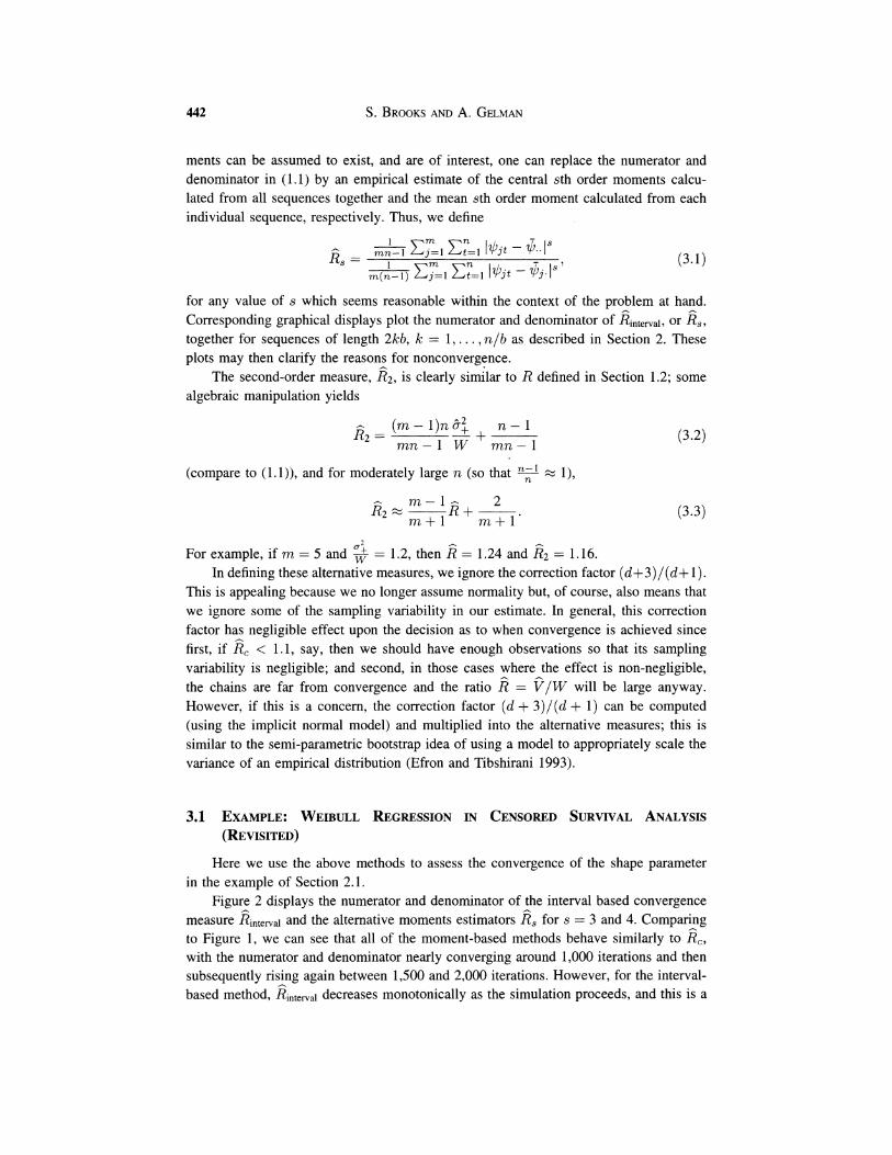
Here we use the above methods to assess the convergence of the shape parameter in the example of Section 2.1.

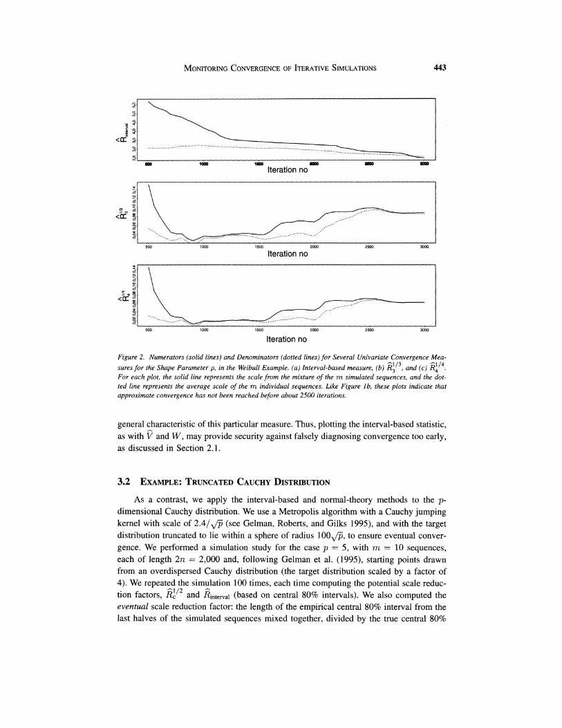
Figure 2 displays the numerator and denominator of the interval based convergence A

measure Rinterv,land the alternative moments estimators R, for s = 3 and 4. Comparing to Figure 1, we can see that all of the moment-based methods behave similarly to E,, with the numerator and denominator nearly converging around 1,000 iterations and then subsequently rising again between 1,500 and 2,000 iterations. However, for the interval- based method, kinterValdecreases monotonically as the simulation proceeds, and this is a

3

9 1..........,,," ... ' "". ........... :I\-. ....................................... .................. .........................\

1DO f a 4 f r n om0 won om0 lteration no

P ........... .....3 . . "

X .... ...'.. . . . . . . . . .... . . . . . . . . . . . . . . 0 . . . . . . . . ............ ........... . . . . . .

500 1OW 1500 2WO 2500 30W lteration no

3 .......... !----__--I J ............: .3 "' .............. . . ......... . . . . . . . ...

....... 500 10W 1500 20W 2500 30W

lteration no

Figure 2. Numerators (solid lines) and Denominators (dotted lines) for Several Univariate Convergence Mea- sures for the Shape Parameter p, in the Weibull Example. (a ) Interval-based measure, (b ) E:I3,and (c ) Ei'4. For each plot, the solid line represents the scale from the mixture of the m simulated sequences, and the dotted line represents the average scale of the m individual sequences. Like Figure lb , these plots indicate that approximate convergence has not been reached before about 2500 iterations.

general characteristic of this particular measure. Thus, plotting the interval-based statistic, as with and W, may provide security against falsely diagnosing convergence too early, as discussed in Section 2.1.

As a contrast, we apply the interval-based and normal-theory methods to the p-dimensional Cauchy distribution. We use a Metropolis algorithm with a Cauchy jumping kernel with scale of 2.4/@ (see Gelman, Roberts, and Gilks 1995), and with the target distribution truncated to lie within a sphere of radius loo@, to ensure eventual convergence. We performed a simulation study for the case p = 5, with m = 10 sequences, each of length 2n = 2,000 and, following Gelman et al. (1995), starting points drawn from an overdispersed Cauchy distribution (the target distribution scaled by a factor of 4). We repeated the simulation 100 times, each time computing the potential scale reduc-

A

tion factors, EL'* and RinterVal(based on central 80% intervals). We also computed the eventual scale reduction factor: the length of the empirical central 80% interval from the last halves of the simulated sequences mixed together, divided by the true central 80%

interval from the target distribution. For simplicity, we consider the convergence of just one parameter-the first element of the p-dimensional vector parameter.

In this example, which is far from normal, we were surprised to find that the normal- based convergence diagnostic performs much better than the interval-based measure. One way to see this is to classify the simulations by whether the potential scale reduction factor is greater or less than 1.2, which is sometimes used as a guideline for "approximate convergence." Of the 100 simulations, 54 had achieved ELI2 < 1.2 at 2;000 iterations and 46 had not. Of the 54 cases with this apparent "convergence," ELI2 ranged from 1.03 to 1.19, and the eventual scale reduction factors, based on the true target distribution, ranged from .6 to 1.6, with only eight cases having eventual scale reduction factors greater than 1.2. Of the 46 simulations in which "convergence" had apparently not been reached, gal2 ranged from 1.2 to 2.1, and the eventual scale reduction factors ranged from .6 to 4.5, with 26 cases having eventual scale reduction factors greater than 1.2. This

-1 / 2performance is not bad for the purposes of monitoring convergence-when R , < 1.2, -1 /2we can be pretty sure that convergence has been reached, but when R, > 1.2, we can

say little. (If we were to adopt the more stringent standard of g;" < 1.1, we would find that 21 out of the 100 simulations reached convergence, and, reassuringly, 20 of these had eventual scale reduction factors below 1.1.)

A

In contrast, Ri,te,,,l is often wildly optimistic in this example. All 100 of our simulations reported gi,,,,,,l < 1.2, even though, as noted previously, in 34 of the cases, the eventual scale reduction was greater than 1.2, with a high of 4.5. The corrected version, [(d+3 ) / ( d + 1 ) ] 1 / 2 ~ i , t e , v , 1 ,is not much better: 93 of the simulations yield a value below 1.2, and 28 of these have eventual scale reductions greater than 1.2, with a high of 3.1.

Why is this happening? This is an example in which a large number of simulation draws-even if obtained independently, rather than via MCMC-are needed to accurately estimate the mean, variance, and 80% interval of the target distribution. The 80% intervals from each individual sequence are themselves far more variable than from the mixture of all 10 sequences. The sampling distribution of interval widths is skewed in the positive

A

direction, so that the denominator of Rintervaltends to be larger than its numerator. In fact, in 98 of the 100 simulations above, gi,,,,,l was less than 1 , and in 67 of the simulations, ( ( d+ 3 ) / ( d+ 1))1/26i,,e,,,lwas less than 1. In general, this suggests that if the interval method is used, it is not necessarily appropriate to combine the widths of individual sequences by simple averaging.

Incidentally, the convergence diagnostic based on empirical coverage probabilities performs well in this example. In our 100 simulations, the average empirical coverage probabilities (ECP's) of the nominal 80% intervals ranged from .62 to .79, and they were highly predictive of the eventual (true) scale reduction factors: all of the simulations for which the ECP was less than .70 had eventual SRF's greater than 1.2; of the simulations for which the ECP was between .70 and .75, 58% had eventual SRF's greater than 1.2; and of the simulations for which the ECP was between .75 and .80 (i.e., quite close to the nominal coverage probability of .80), only 3% had eventual SRF's greater than 1.2.

Despite the problems with the interval-based PSRF, we emphasise that our methods have not "failed" in this example, because we would recommend using the alternative measures in addition to the traditional g, and not accepting convergence until all the measures are satisfied.

Thus, we might plot the original kcstatistic, together with the corresponding numer- A

ator and denominator ( c and W) and the diagnostic. The Rc provides us with a scale for the diagnostic, which is interpretable in terms of the utility of continuing to run the chain, whereas the other plots, provide some reassurance against falsely diagnosing convergence too early; that is, the and W plots should both settle down and to the same location before convergence is diagnosed. The idea is to use a wide variety of diagnostics so that if all appear to suggest that convergence has been achieved, then the user can have some confidence in that conclusion. Having discussed these univariate extensions to the original method, we now move on to discuss an extension of the original method to the case where we are interested not in scalar functionals, but more general multivariate functionals of the chain.

4. MULTIVARIATE EXTENSIONS There are a number of multivariate approaches available to us. When we are inter-

ested in the estimation of a vector parameter $ based upon observations $$:) denoting the ith element of the parameter vector in chain j at time t , the direct analogue of the univariate approach in higher dimensions is to estimate the posterior variance-covariance matrix by

where

and

denote the @-dimensional) within and between-sequence covariance matrix estimates of the p-variate functional $, respectively. Thus, we can monitor both and W, determining convergence when any rotationally invariant distance measure between the two matrices indicates that they are "sufficiently" close.

Before we go on to discuss scalar measure of distance between the and W matri-ces, we should point out that similar extensions can also be provided to the alternative diagnostics proposed in Section 3. In particular, the interval-based diagnostic in the univariate case becomes a comparison of volumes of total and within-chain convex hulls. Thus, for each chain we calculate the (hyper-)volume within 95%, say, of the points in the sample and compare the mean of these with the volume from 95% of the observations from all samples together. However, such a method is likely to be computationally expensive in even moderate dimensions, so we have not adopted this approach here.

We would like to summarize the distance between P and W with a scalar measure which should approach 1 (from above) as convergence is achieved, given suitably over-dispersed starting points. Many such measures can be constructed; we will work with the maximum root statistic, which is the maximum SRF of any linear projection of $, given by

- max a l P aR p = a -a l W a '

which we call the multivariate PSRF (or MPSRF) and which we can compute via the following lemmas.

Lemma 1. For two nonsingular, positive definite and symmetric matrices M and N ,

max a l M a a -= a l N a A,

where X is the largest eigenvalue of the positive definite matrix N - ' M Proof: See Mardia, Kent, and Bibby (1979, sec. A.9.2).

Lemma 2.

where XI is the largest eigenvalue of the symmetric, positive definite matrix W-' ~ / n . Proof:

Ep = max alQa a -a l W a

by Lemma 1. Clearly, under the assumption of equal means between sequences, XI -+ 0 and so

@' tends to 1 for reasonably large n. Note that these measures are incalculable in the case where W is singular. If both

W and B are singular, then this suggests that the underlying problem is ill-posed, for example two or more parameters may be very highly correlated. However, if only W is singular, then this suggests that the problem lies with the sampler; for example, one or more variables have failed to move within the current set of iterations. Thus, in the case where EP is incalculable, due to the singularity of W, we still gain valuable information by examining the determinants of both the B and W matrices. Another instance in which

the bound may be incalculable is if the matrix is too large to invert or decompose. This is essentially a constraint imposed by the hardware available and we have yet to try a model where this has been a problem.

In order to monitor the three conditions for convergence described in Section 2, we might also monitor plots of the determinants of, say, the pooled and within chain covariance matrices, which should stabilize as a function of n. Thus, the multidimensional approach involves monitoring one (or more) of the measures above, together with the determinants say, of the pooled and within chain covariance matrices.

One reason for choosing Ep among all the possible multivariate generalizations of the SRF is that it may be used as an approximate upper bound to the maximum of the univariate E statistics over all p variables.

Lemma 3. For k = 1 , .. . , p, let Z ( k ) be the univariate PSRF defined in (1.1), applied to the simulations of the kth element of 8. If Emaxdenotes the maximum of the 6 ( k ) values (over k = 1, . . . .p ) then,

where EP is the MPSRF defined in (4.1), applied to the vector of parameters, 8. Proof: Let Ik denote a vector of zeroes, with kth entry replaced by 1. Then

max a l P aEp = a -a l W a

max = k E ( k )

Thus, the multivariate measure 6 p is an upper bound to the largest of the original measures over each of the elements of 8.

4.3.1 Example: Weibull Regression in Censored Survival Analysis (Revisited)

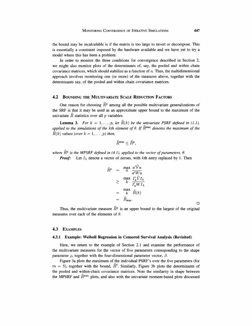
Here, we return to the example of Section 2.1 and examine the performance of the multivariate measures for the vector of five parameters corresponding to the shape parameter p, together with the four-dimensional parameter vector, P.

Figure 3a plots the maximum of the individual PSRF's over the five parameters (for m = 5), together with the bound, E5. Similarly, Figure 3b plots the determinants of the pooled and within-chain covariance matrices. Note the similarity in shape between the MPSRF and Emaxplots, and also with the univariate moment-based plots discussed

-500 1000 1500 2000 2500 3000 Iteration no

(b)

Iteration no ,.. A

Figure 3. (a ) Plots of maximum of the individual PSRF's (Rmax , solid) together with bound based upon R 5 (dotted). (b ) Plot of the the determinants ( x lo6) of the pooled (solid) and within-chain (dotted) covariance matrices.

earlier. Like the PSRF's, the MPSRF plot also possesses a second peak after about 2,000 iterations.

In this case we can clearly see how the MPSRF bounds above the Emaxdiagnostic, with E5= 1.5 x Emaxwithin iterations 1-3,000. Obviously, this bound improves as the simulations continue, since the MPSRF itself also converges to 1. Figure 3a illustrates that monitoring the MPSRF may well cause us to diagnose convergence later than the univariate PSRF plots. This difference is essentially a measure of the lack of convergence attributed to the interaction between the scalar functionals that we have chosen to study.

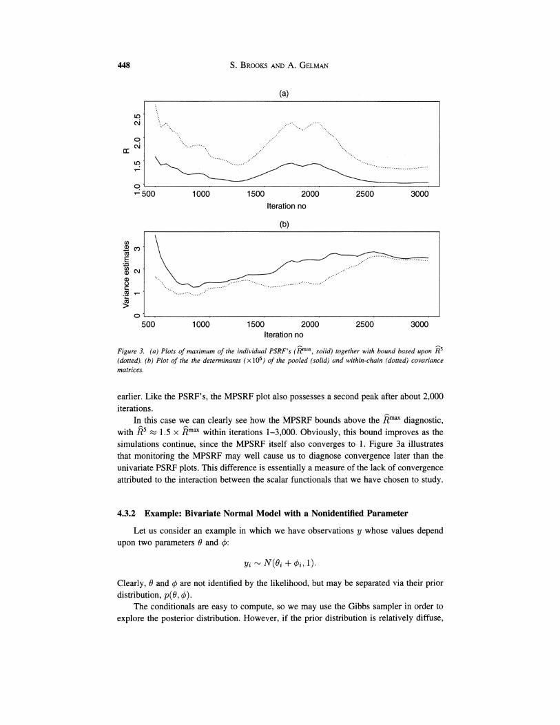
4.3.2 Example: Bivariate Normal Model with a Nonidentified Parameter

Let us consider an example in which we have observations y whose values depend upon two parameters B and 4:

Clearly, 6' and 4 are not identified by the likelihood, but may be separated via their prior distribution, p(Q,4).

The conditionals are easy to compute, so we may use the Gibbs sampler in order to explore the posterior distribution. However, if the prior distribution is relatively diffuse,

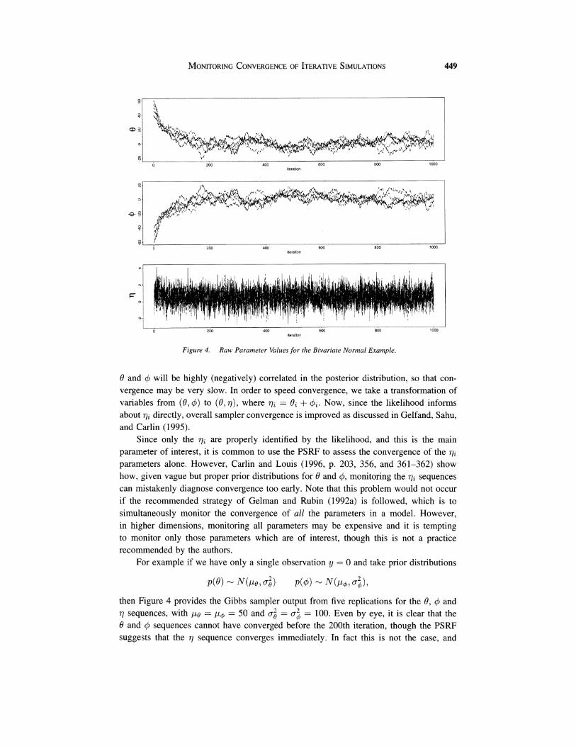
Figure 4. Raw Parameter Values for the Bivariate Normal Example.

0 and Q will be highly (negatively) correlated in the posterior distribution, so that convergence may be very slow. In order to speed convergence, we take a transformation of variables from ( 0 . 4 ) to ( 0 . q ) , where 77% = 8t + G2.Now, since the likelihood informs about q, directly, overall sampler convergence is improved as discussed in Gelfand, Sahu, and Carlin (1995).

Since only the 7 , are properly identified by the likelihood, and this is the main parameter of interest, it is common to use the PSRF to assess the convergence of the 7 , parameters alone. However, Carlin and Louis (1996, p. 203, 356, and 361-362) show how, given vague but proper prior distributions for Q and d, monitoring the q, sequences can mistakenly diagnose convergence too early. Note that this problem would not occur if the recommended strategy of Gelman and Rubin (1992a) is followed, which is to simultaneously monitor the convergence of all the parameters in a model. However, in higher dimensions, monitoring all parameters may be expensive and it is tempting to monitor only those parameters which are of interest, though this is not a practice recommended by the authors.

For example if we have only a single observation y = 0 and take prior distributions

then Figure 4 provides the Gibbs sampler output from five replications for the 0, 0 and 7 sequences, with = po = 50 and a; = o: = 100. Even by eye, it is clear that the 0 and q5 sequences cannot have converged before the 200th iteration, though the PSRF suggests that the 7 sequence converges immediately. In fact this is not the case, and

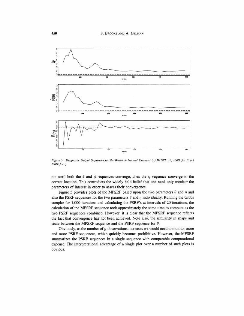
Figure 5. Diagnostic Output Sequences for the Bivariare Normal Example. ( a ) MPSRF. (b)PSRF for 0. (c ) PSRF for 17.

not until both the 0 and q5 sequences converge, does the 77 sequence converge to the correct location. This contradicts the widely held belief that one need only monitor the parameters of interest in order to assess their convergence.

Figure 5 provides plots of the MPSRF based upon the two parameters 0 and 77 and also the PSRF sequences for the two parameters 0 and 77 individually. Running the Gibbs sampler for 1,000 iterations and calculating the PSRF's at intervals of 20 iterations, the calculation of the MPSRF sequence took approximately the same time to compute as the two PSRF sequences combined. However, it is clear that the MPSRF sequence reflects the fact that convergence has not been achieved. Note also, the similarity in shape and scale between the MPSRF sequence and the PSRF sequence for 0.

Obviously, as the number of y-observations increases we would need to monitor more and more PSRF sequences, which quickly becomes prohibitive. However, the MPSRF summarizes the PSRF sequences in a single sequence with comparable computational expense. The interpretational advantage of a single plot over a number of such plots is obvious.

20000 40000 60000 80000 100000

Iteration No

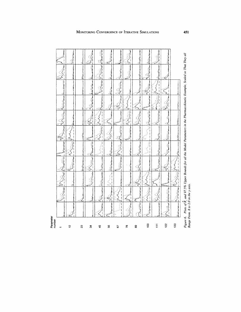
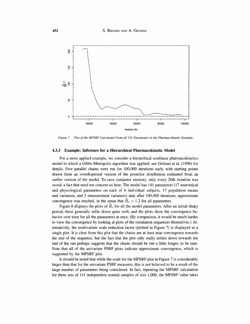
Figure 7 Plot of the MPSRF Calculated From all 141 Parameters in the Pharmacokinetic Example

4.3.3 Example: Inference for a Hierarchical Pharmacokinetic Model

For a more applied example, we consider a hierarchical nonlinear pharmacokinetics model to which a Gibbs-Metropolis algorithm was applied; see Gelman et al. (1996) for details. Five parallel chains were run for 100,000 iterations each, with starting points drawn from an overdispersed version of the posterior distribution estimated from an earlier version of the model. To save computer memory, only every 20th iteration was saved, a fact that need not concern us here. The model has 141 parameters (17 anatomical and physiological parameters on each of 6 individual subjects, 17 population means and variances, and 5 measurement variances) and, after 100,000 iterations, approximate convergence was reached, in the sense that g,< 1.2 for all parameters.

Figure 6 displays the plots of gcfor all the model parameters. After an initial shaky period, these generally settle down quite well, and the plots show the convergence behavior over time for all the parameters at once. (By comparison, it would be much harder to view the convergence by looking at plots of the simulation sequences themselves.) Al- ternatively, the multivariate scale reduction factor (plotted in Figure 7) is displayed as a single plot. It is clear from this plot that the chains are at least near convergence towards the end of the sequence, but the fact that the plot only really settles down towards the end of the run perhaps suggests that the chains should be run a little longer, to be sure. Note that all of the univariate PSRF plots indicate approximate convergence, which is supported by the MPSRF plot.

It should be noted that while the scale for the MPSRF plot in Figure 7 is considerably larger than that for the univariate PSRF measures, this is not believed to be a result of the large number of parameters being considered. In fact, repeating the MPSRF calculation for three sets of 141 independent normal samples of size 1,000, the MPSRF value takes

values no larger than 1.3. This suggests that the MPSRF plots should be considered to be on a similar scale to the univariate PSRF plots and that, in general, large values of the MPSRF statistic suggests real problems in the convergence of functions of the parameters other than the individual parameters themselves. Thus, the large scale for the MPSRF plot in Figure 7 suggests that, at the very least, if we are interested in quantities besides the 141 parameters individually, then it might also be sensible to examine their PSRF's.

5. DISCUSSION The aim of this article has been to suggest a number of alternative implementations

of the original convergence diagnostic proposed by Gelman and Rubin (1992a). Clearly an iterative approach introduces a qualitative element to the original method, providing us with information on how the chains are converging. Such an approach can be applied to all the methods we discuss in this article.

The original approach can be immediately generalized to other summaries beyond second moments, thus losing the restrictive normality assumption while retaining the desirable properties of the method (most notably, that 6 converges to 1 as the simulations mix). In many problems, it would be most appropriate to apply a battery of convergence tests based on the sorts of inferences that are of interest in the ultimate output of the simulations. However, the interval-based approach can be "over-optimistic," particularly in the case of skewed distributions, as shown in the example of the Cauchy distribution. Once a simulation is judged to be well-mixed (as measured by the PSRF's), it makes sense to examine the plots of their numerators and denominators, to verify that the "between" variation is decreasing and the "within" variation is increasing as the simulations converge. For higher dimensional problems, the MPSRF has a distinct advantage in terms of its interpretability, summarizing the individual PSRF's and providing a bound on them as the chains converge. Verification of the MPSRF may also be obtained by plotting the relevant determinants.

We have discussed how each of the extensions of the original method provide safe- guards against false diagnosis of convergence under different situations. However, all methods based solely upon sampler output can be fooled (see Asmussen, Glynn, and Tho- risson 1992), and multiple-chain-based diagnostics, while safer than single-chain-based diagnostics, can still be highly dependent upon the starting points of the simulations.

Having said that, we believe that, in practice, it may be useful to combine a number of the alternative approaches proposed in this article in diagnosing convergence. For example, for high dimensional problems, the MPSRF may be calculated, together with the PSRF's for each of the parameters of interest, which might also be combined with plots of the determinants of the covariance matrices and estimated variances, respectively. Note the distinction between this "cocktail" of diagnostics and simply plotting the PSRF's for parameters of interest alone. In combining a number of approaches, the strengths of each of the approaches may be combined, and some reliability may be placed on the conclusions thus drawn.

ACKNOWLEDGMENTS The authors thank Gareth Roberts, Xiao-Li Meng, Phillip Price, three anonymous referees and an associate

editor for helpful comments. We also thank the U.S. National Science Foundation for grant DMS-9404305 and Young Investigator Award DMS-9457824, the U.K. Engineering and Physical Sciences Research Council, and the Research Council of Katholieke Universiteit Leuven for fellowship F19619.

[Received September 1996. Revised October 1997.1

REFERENCES Applegate, D., Kannan, R., and Polson, N. G. (1990), "Random Polynomial Time Algorithms for Sampling

from Joint Distributions," technical report no. 500, Carnegie-Mellon University. Asmussen, S., Glynn, P. W., and Thorisson, H. (1992), "Stationarity Detection in the Initial Transient Problem,"

ACM Transactions on Modelling and Computer Simulation, 2, 130-157. Brooks, S. P., and Roberts, G. 0 . (in press), "Diagnosing Convergence of Markov Chain Monte Carlo Algo-

rithms," Statistics and Computing. Carlin, B. P., and Louis, T. A. (1996), Bayes and Empirical Bayes Methods for Data Analysis, London: Chapman

and Hall. Cowles, M. K., and Carlin, B. P. (1996), "Markov Chain Monte Carlo Convergence Diagnostics: A Comparative

Review," Journal of the American Statistical Association, 91, 883-904. Dellaportas, P., and Smith, A. F. M. (1993), "Bayesian Inference for Generalized Linear and Proportional

Hazards Models via Gibbs Sampling," Applied Statistics, 42, 443-460. Efron, B., and Tibshirani, R. J. (1993), An Introduction to the Bootstrap, New York: Chapman and Hall. Fisher, R. A. (1935), The Design of Experiments, Edinburgh: Oliver and Boyd Gelfand, A. E., Sahu, S. K., and Carlin, B. P. (1995), "Efficient Parameterizations for Normal Linear Mixed

Models," Biometrika, 82, 479488. Gelfand, A. E., and Smith, A. F. M. (1990), "Sampling Based Approaches to Calculating Marginal Densities,"

Journal of the American Statistical Association, 85, 398-409. Gelman, A., F., Bois, Y., and Jiang, J. (1996), "Physiological Pharmacokinetic Analysis using Population

Modelling and Informative Prior Distributions," Journal of the American Statistical Association, 91, 1400- 1412.

Gelman, A,, Roberts, G. O., and Gilks, W. R. (1995), "Efficient Metropolis Jumping Rules," in Bayesian Statistics 5, eds. J. M. Bernardo, J. 0 . Berger, A. P. Dawid, and A. F. M. Smith, New York: Oxford University Press, pp. 599-608.

Gelman, A,, and Rubin, D. (1992a), "Inference from Iterative Simulation using Multiple Sequences," Statistical Science, 7, 457-5 1 1. -(1992b), "A Single Series from the Gibbs Sampler Provides a False Sense of Security," in Bayesian

Statistics 4 , eds. J. M. Bernardo, J. 0 . Berger, A. P. Dawid and A. F. M. Smith, New York: Oxford University Press, pp. 625-631.

Gilks, W. R., Richardson, S., and Spiegelhalter, D. J. (1996), Markov Chain Monte Carlo in Practice, London: Chapman and Hall.

Green, E. J., Roesch, F. A,, Smith, A. F. M., and Strawderman W. E. (1994). "Bayesian Estimation for the Three Parameter Weibull Distribution with Tree Diameter Data," Biometrics, 50, 254-269.

Grieve, A. P. (1987), "Applications of Bayesian Software: Two Examples," Statistician, 36, 283-288. Jennison, C. (1993), Discussion of "Bayesian Computation via the Gibbs Sampler and Related Markov Chain

Monte Carlo Methods," by Smith and Roberts, Journal of the Royal Statistical Societ).', Series B, 55, 54-56.

Liu, C., and Rubin, D. B. (in press), "Markov-Normal Analysis of Iterative Simulations Before Their Conver- gence," Journal of Econometrics.

Mardia, K. V., Kent, J. T., and Bibby, J. M. (1979), Multivariate Analysis, London: Academic Press.

Rosenthal, J. S. (1995), "Minorization Conditions and Convergence Rates for Markov Chain Monte Carla," Journal of the American Statistical Association, 90, 558-566.

Tanner, M., and Wong, W. (1987), "The Calculation of Posterior Distributions by Data Augmentation," Journal of the American Statistical Association, 82, 528-550.

Tiemey, L. (1994), "Markov Chains for Exploring Posterior Distributions," The Annals of Statistics, 22, 1701-1762.

Yu, B. (1995), Discussion of "Bayesian Computation and Stochastic Systems," by Besag et al. (1995), Statistical Science, 10, 3-66.

general methods for monitoring convergence of iterative...

Documents