multiple - bris.ac.uk
TRANSCRIPT

Multiple membership multiple classi�cation
�MMMC� models
William J� Browne�� Harvey Goldstein and Jon Rasbash
Institute of Education� University of London� �� Bedford Way�
London WC�H �AL� UK
Summary
In the social and other sciences many data are collected with a known butcomplex underlying structure� Over the past two decades there has beenan increase in the use of multilevel modelling techniques that account fornested data structures� Often however the underlying data structures aremore complex and cannot be �tted into a nested structure� First there arecross�classi�ed models where the classi�cations in the data are not nested�Secondly we consider multiple membership models where an observationdoes not belong simply to one member of a classi�cation� These two ex�tensions when combined allow us to �t models to a large array of under�lying structures� Existing frequentist modelling approaches to �tting suchdata have some important computational limitations� In this paper we con�sider ways of overcoming such limitations using Bayesian methods� sinceBayesian model �tting is easily accomplished using Monte Carlo Markovchain �MCMC� techniques� In examples where we have been able to makedirect comparisons� Bayesian methods in conjunction with suitable �di�useprior distributions lead to similar inferences to existing frequentist tech�niques� In this paper we illustrate our techniques with examples in the�elds of education� veterinary epidemiology� demography� and public healthillustrating the diversity of models that �t into our framework�
Keywords� Multilevel Modelling� Hierarchical Modelling� Markov ChainMonte Carlo �MCMC�� Cross classi�ed models� multiple membership mod�els� complex data structures� Bayesian GLMM modelling
� Introduction
Over the past two decades or so there has been a great interest in �ttingrealistically complex statistical models to the large datasets that occur in thesocial sciences and other application areas� These complex models accountfor the underlying structure in such datasets through the use of random

e�ects� Historically some of the �rst random e�ects models �tted to largedatasets were in the �eld of education and here the structures of interest weregenerally pupils within classes within schools and other nested or hierarchicalstructures� The �tting of these multilevel or hierarchical models �eg Goldstein���� �� Bryk and Raudenbush ����� and Draper ������ is now commonplace in many application areas and several special purpose software packageshave been developed to �t such models �Rasbash et al� ����b�� Bryk et al���������
To �t these models it is necessary to use either iterative procedures� forexample iterative generalised least squares �IGLS �Goldstein� ������ or sim�ulation based methods� for example Gibbs sampling �Gelfand and Smith������� Due to the computational intensity of the MCMC simulation basedmethods and the speed of computers at the time� the iterative maximumlikelihood procedures were implemented in software packages �ML �Ras�bash� ������ HLM �Bryk et al�� ������ several years prior to the MCMCmethods�
Those who used these early statistical modelling packages then discovereddatasets whose structures did not �t into the standard multilevel framework�Two such structures are cross�classi�ed models and multiple membershipmodels� Methods like IGLS exploit the nested structure of the data in multi�level �hierarchical� models� As these two types of structures are not strictlynested the initial solution was to convert these structures into nested modelswith constraints �Rasbash and Goldstein� ������ This approach along withits problems will be discussed further in a later section�
In fact such models are part of a larger family of models known as gener�alised linear mixed models �GLMM�� These models are a combination of thelinear mixed model �Harville� ����� and the generalized linear model frame�work �Nelder and Wedderburn� ����� The �normal� linear mixed model canbe written
y � X� � Zu � e�u �MVN������ � e � N��� ��e ��
���
Here the formulation of �� will control the type of mixed model produced�For multilevel modelling u will contain the random e�ects and �� is block di�agonal� i�e� the u are split into independent subsets� one subset for each level�Clayton and Rasbash ������ also consider cross�classi�ed models as a spe�cial case of the GLMM model and use a technique they call the �AlternatingImputation Posterior �AIP� algorithm which we will describe later�
From a Bayesian viewpoint� Clayton ������ shows the �exibility of dif�ferent speci�cations of the random e�ects precision matrix� ���
� � In thispaper the models that we consider will all have block diagonal �� and wewill actually split u into its independent subsets in the equations that follow�Additional complexity� in the form of cross�classi�ed models and multiplemembership models will then be achieved by modi�cations to the Z matrix�

�
We will also later deal with the non�normal GLM case�A serious problem with the increase in complexity of the models is to
establish a notation� particularly for the indices that captures the structureof the models �See Rasbash and Browne� ��� for more details and for anotation that extends the standard multilevel notation�� Nevertheless wewill see that the MCMC methods that we use in this paper do not need toknow the exact nesting structures in the model for estimation purposes� Inthis paper we develop some new terminology and notation that hopefullywill make the equations and estimation algorithms for these complex modelssimpler�
In the next section we introduce these new de�nitions and notation anddemonstrate how they work for a simple two level model� Then in sections� and � we consider the two advances to the basic structure of the multi�level model� namely cross�classi�ed e�ects and multiple�membership mod�els with examples� We then describe our general framework of multiple�membership multiple classi�cation �MMMC� models that encompasses thesetwo advances� We �nally demonstrate through three actual data examplesthe kinds of models that can be �tted in this framework�
� Classi�cations
Consider a problem that has one response variable �multivariate responsesare a simple extension� and assume that there is a unique response in ourdataset for each of N lowest level units� Here the lowest level units could beindividuals� time points or even areas�
We now de�ne a classi�cation as a function� c� that maps from the set� of N lowest level units to a set � of size M where M � N � and we de�nethe resulting set � of M objects as the classi�cation units� So we havec�ni� � �i� where the lowest level unit ni � � and �i � ��
We will consider two types of classi�cations� A single membership
classi�cation is a function c from � to � that maps each ni � � to aunique mj � �� A multiple membership classi�cation is a map c from� to � that maps each ni � � to a subset �possibly of size �� �i of �� Notethat we will still maintain that M � N to avoid identi�ability problems inthe estimation that follows�
A special classi�cation is the identity classi�cation that maps every ni � �to ni � � where � � �� Given these de�nitions we will now see that allthe sets of random e�ects that feature in multilevel models� cross�classi�edmodels and multiple membership models will each have an associated clas�si�cation� Note that di�erent classi�cations may share the same set � ofclassi�cation units� for example the areas and neighbours classi�cations inthe lip cancer example in section ��
�
��� The importance of unique identi�ers in nested mod�els
One potential problem in �tting multilevel �hierarchical� models in the frame�work that we are introducing is the problem of unique identi�ers� For examplein education� a very common structure is to have pupils within classes withinschools� Here we could have class � in school � and class � in school � Hier�archical data structures are in fact a special case of the cross�classi�ed datastructures that we study next that have no crossings� Therefore we could �t ahierarchical model as a cross�classi�ed model� however in this case we wouldneed to di�erentiate between the two class �s as they are not the same classi��cation unit� We shall therefore assume that all classi�cation unit identi�ersare unique across a dataset�
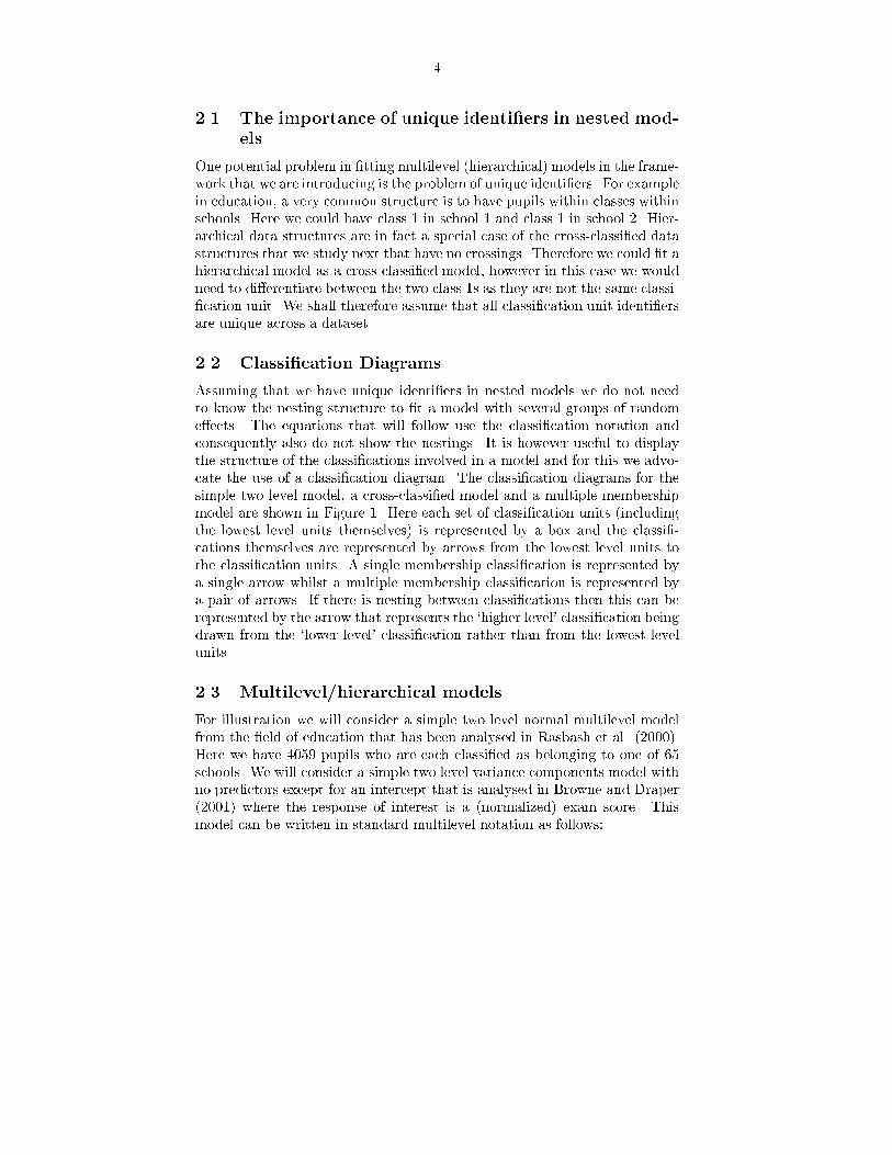
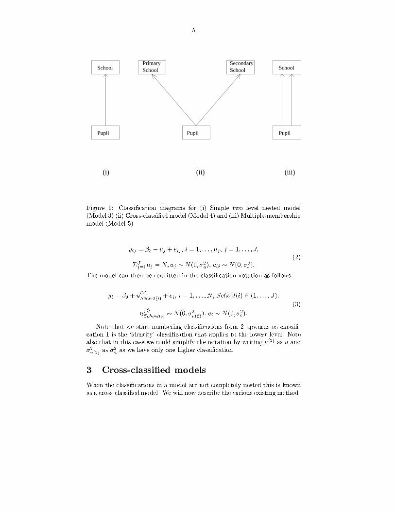
��� Classi�cation Diagrams
Assuming that we have unique identi�ers in nested models we do not needto know the nesting structure to �t a model with several groups of randome�ects� The equations that will follow use the classi�cation notation andconsequently also do not show the nestings� It is however useful to displaythe structure of the classi�cations involved in a model and for this we advo�cate the use of a classi�cation diagram� The classi�cation diagrams for thesimple two level model� a cross�classi�ed model and a multiple membershipmodel are shown in Figure �� Here each set of classi�cation units �includingthe lowest level units themselves� is represented by a box and the classi��cations themselves are represented by arrows from the lowest level units tothe classi�cation units� A single membership classi�cation is represented bya single arrow whilst a multiple membership classi�cation is represented bya pair of arrows� If there is nesting between classi�cations then this can berepresented by the arrow that represents the �higher level classi�cation beingdrawn from the �lower level classi�cation rather than from the lowest levelunits�
��� Multilevel�hierarchical models
For illustration we will consider a simple two level normal multilevel modelfrom the �eld of education that has been analysed in Rasbash et al� ������Here we have �� � pupils who are each classi�ed as belonging to one of � schools� We will consider a simple two level variance components model withno predictors except for an intercept that is analysed in Browne and Draper����� where the response of interest is a �normalized� exam score� Thismodel can be written in standard multilevel notation as follows�
Pupil
School
(i)
Pupil
PrimarySchool
SecondarySchool
(ii)
Pupil
School
(iii)
Figure �� Classi�cation diagrams for �i� Simple two level nested model�Model �� �ii� Cross�classi�ed model �Model �� and �iii� Multiple�membershipmodel �Model ��
yij � �� � uj � eij � i � �� � � � � nj � j � �� � � � � J�
�Jj��nj � N� uj � N��� ��u�� eij � N��� ��e��
��
The model can then be rewritten in the classi�cation notation as follows�
yi � �� � u���School�i� � ei� i � �� � � � � N� School�i� � ��� � � � � J��
u���School�i� � N��� ��u����� ei � N��� ��e��
���
Note that we start numbering classi�cations from upwards as classi��cation � is the �identity classi�cation that applies to the lowest level� Notealso that in this case we could simplify the notation by writing u��� as u and��u��� as ��u as we have only one higher classi�cation�
� Cross�classi�ed models
When the classi�cations in a model are not completely nested this is knownas a cross�classi�ed model� We will now describe the various existing method�

�
ologies for �tting cross�classi�ed models before considering an example�
��� Alternative Methodology
There are several frequentist approaches that have been considered for �ttingcross�classi�ed models� In the examples that follow we will only compare theapproach of Rasbash and Goldstein ������ with a corresponding Bayesianmodel �t accomplished via MCMC� but will list the other approaches forcompleteness�
Rasbash and Goldstein ������ describe a likelihood�based approach thatinvolves transforming the cross�classi�ed model into a constrained nestedmodel� Then the standard IGLS algorithm can be used to �t the result�ing constrained model� For datasets with large numbers of units in eachclassi�cation this approach requires large amounts of memory to cope withthe constraints� Also for examples that deviate away from a close to nesteddesign there can be numerical instabilities in the method�
Clayton and Rasbash ������ introduced a technique that uses a dataaugmentation approach �Tanner and Wong ����� Schafer ������ Their Al�ternating Imputation Prediction �AIP� method consists of treating the vari�ous nested hierarchies ��wings in their terminology� in turn whilst includingterms from the other �wings as o�set terms� For each �wing a maximumlikelihood or quasi�likelihood method is used and then a stochastic draw ofthe residuals is taken� Although this method works reasonably well� if the re�sponse is a binary variable and quasi�likelihood methods need to be used� thenthis method is still a�ected by the bias that is inherent in quasi�likelihoodmethods for binary response multilevel models �See Goldstein and Rasbash������
Raudenbush ������ considers an empirical Bayes approach to �tting cross�classi�ed models based on the EM algorithm� He considers the speci�c caseof two classi�cations where one of the classi�cations has many units whilstthe other has far fewer and shows two educational examples to illustrate themethod�
Two other recent approaches that can be used for �tting cross�classi�edmodels� in particular with non�normal responses are Gauss�Hermite quadra�ture within PQL estimation �Pan and Thompson ���� and the HGLM modelframework as described in Lee and Nelder ������ Neither of these approacheshas been designed with speed of estimation in mind and so they are currentlynot feasible for the size of some of the problems that we will consider in thispaper�
The MCMC algorithms for cross�classi�ed models using the classi�cationnotation above are essentially identical to the algorithms for a nested model�as the MCMC method treats each classi�cation as a random additive termand does not need to construct the global block�diagonal V matrix used in theIGLS algorithm� We are implementing the MCMC approach as a Bayesianmethod and consequently in the models that follow we will need to add

�
prior distributions for unknown parameters� In order to compare with themaximum likelihood based IGLS method �and because we have no additionalprior information� we will use di�use prior distributions in all the examplesthat follow� Note that unless otherwise stated in all the models that followwe use Normal������� priors for all �xed e�ects and ������ �� priors for allvariance components where � � �����
MCMC methods have an important advantage over the IGLS algorithmin that� as they are simulation�based� they produce estimates of the wholeposterior distributions of the unknown parameters rather than just pointestimates and standard errors�
��� An example
The data that we will consider come from Fife in Scotland� As a responsevariable we have the exam results at age �� of ���� school children whoattended �� secondary schools and ��� primary schools� Here there is across�classi�cation of primary schools and secondary schools since not everychild who went to a particular primary school then proceeded to the samesecondary school� Often in education particular primary schools are feederschools to a particular secondary school� In our example �� out of ��� primaryschools had children who went to di�erent secondary schools� If we de�nethe main secondary school for primary school i� as the secondary school towhich the largest number of pupils in school i attended� then we �nd thatonly �� out of ���� children went to a secondary other than their mainsecondary� So although we have a cross�classi�ed design� the distribution ofpupils is close to nested�
We will �t the following simple cross�classi�ed variance components modelto the dataset
yi � �� � u���SEC�i� � u
���PRIM�i� � ei�
u���SEC�i� � N��� ��u����� u
���PRIM�i� � N��� ��u�����
ei � N��� ��e ��
���
where yi is the exam score for the ith pupil in the dataset� SEC�i� is thesecondary school they attended and PRIM�i� the primary school they at�
tended� u���SEC�i� is the random e�ect for secondary school SEC�i�� u
���PRIM�i�
is the random e�ect for primary school PRIM�i� and ei is a level � residualfor the ith pupil in the dataset� This model is illustrated in the second clas�si�cation diagram in Figure �� To complete the Bayesian speci�cation of thismodel for the MCMC method we include �di�use priors as described earlier�
We see in Table � that in this example there is more variation betweenprimary schools than between secondary schools� The MCMC �posteriormean� estimates �based on a main run of ����� iterations after a burn�in

�
Table �� Point estimates for the Fife educational dataset�
Parameter IGLS MCMCMean achievement ���� � � ������ � � ������
Between secondary school variance ���u���� ��� ������ ���� �����
Between primary school variance ���u���� ��� ����� ��� �����
Between individual variance ���e � ���� ����� ��� �����
of �� iterations from a simple special case of the algorithm in appendix A�replicate the IGLS estimates from the Rasbash and Goldstein������ methodwith slightly greater higher level variances due to the skewness of the posteriordistribution� A further discussion of this dataset is given in Goldstein���� ��
� Multiple membership models
Our second extension to the standard multilevel framework considers the casewhen a lowest level unit is a member of more than one higher classi�cationunit� These models are commonly known as multiple membership models�Hill and Goldstein ����� Rasbash and Browne ����� For example� in medi�cal studies a hospital patient may be treated by several nurses and each nursewill then have an e�ect on the patients progress� Of course di�erent nurseswill spend di�erent amounts of time with each patient and so we would alsolike to incorporate this information in our model� To do this we use a weight�ing scheme so that for the nurse classi�cation each patient will have weightsfor all the nurses that treated them that typically sum to �� One obviousway of choosing weights would be to make them proportional to the lengthof time each nurse spends with a patient�
Other examples where we may have a multiple membership model are ineducation with children being taught by several teachers in the process oftheir schooling� and in demography where individuals will belong to severaldi�erent households over a period of time�
��� A simulated example
Here we will consider a simulation of a realistic educational example based onthe educational hierarchical dataset �Rasbash et al� ���a� described earlier�We will assume that ��� of children stayed in the same school throughouttheir schooling and that the other ��� changed school �to another schoolchosen at random� at some point during this period� For the purposes of thissimulation we will assume that a child only changes school at most once andthat both schools they are members of are given equal weighting ��� each��

�
Table � Summary of simulations for a simple multiple membership model�
Parameter True IGLS est� �MCSE� MCMC est� �MCSE�Mean achievement ���� � ������� �������� ������� ��������School variance ���
u���� ��� ����� �������� ���� ��������
Individual variance ���e � ��� ����� ������� ����� ��������Actual coverage of nominal ����� � intervalsMean achievement ���� � ����������� �����������School variance ���
u���� � ���������� �����������
Individual variance ���e � � ����������� �����������
Neither of these restrictions are necessary which will become clear in the realdata examples in a later section�
The model is then as follows �
yi � �� �P
j�School�i� w���i�j u
���j � ei�
i � �� � � � � N� School�i� � ��� � � � � J��
u���j � N��� ��u����� ei � N��� ��e��
� �
and is shown in the third classi�cation diagram in Figure �� Again for theMCMC method� we will use di�use prior distributions� As the multiple mem�bership model is a special case of the family of models introduced in the nextsection� the MCMC algorithm here is a Gibbs sampler that is a special caseof the algorithm given in Appendix A�
One thousand sets of response variables were generated with known pa�rameters and the results obtained from the Rasbash and Goldstein IGLSmethod and MCMC with the above priors for this simulation experimentare shown in Table � Here the estimates given by the two methods are theaverage values over the ���� simulated datasets� The ��� interval estimatesfor the MCMC method were constructed from the th and � th percentilesof the chains� whilst for IGLS we used symmetric point estimate ����� esti�mated standard deviation intervals �see Browne and Draper� ��� for similarsimulations on a variance components model�� In Table we see that ourMCMC method gives both very little bias and far better coverage propertiesthan the IGLS method for this model�
��
� Multiple membership multiple classi�cation�MMMC models
�� A general three classi�cation normal model with onemultiple�membership classi�cation
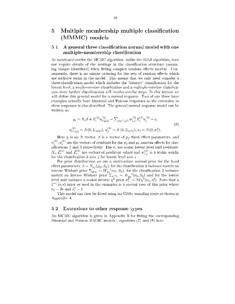
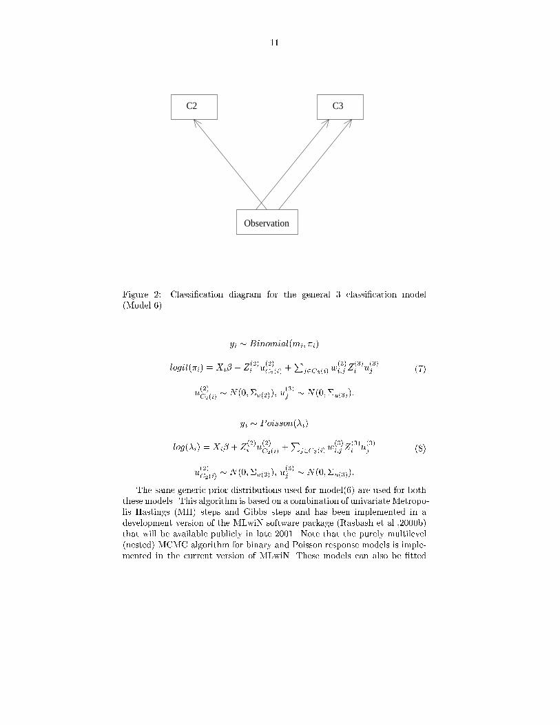
As mentioned earlier the MCMC algorithm� unlike the IGLS algorithm� doesnot require details of the nestings in the classi�cation structure �assum�ing unique identi�ers� when �tting complex random e�ects models� Con�sequently� there is no unique ordering for the sets of random e�ects whichare additive terms in the model� This means that we only need consider athree�classi�cation model which includes the �identity classi�cation for thelowest level� a single�member classi�cation and a multiple�member classi�ca�tion since further classi�cations will involve similar steps� In this section wewill de�ne this general model for a normal response� Two of our three laterexamples actually have binomial and Poisson responses so the extension tothese responses is also described� The general normal response model can bewritten as�
yi � Xi� � Z���i u
���C��i�
�P
j�C��i�w���i�j Z
���i u
���j � ei
u���C��i�
� N����u����� u���j � N����u����� ei � N��� ��e��
���
Here y is an N vector� � is a vector of pf �xed e�ect parameters� and
u���i � u
���i are the vectors of residuals for the p� and p� random e�ects for clas�
si�cations and � respectively� The ei are scalar lowest level unit residuals�
Xi� Z���i and Z
���i are vectors of predictor values and w
���i�j is a scalar weight
for the classi�cation � unit j for lowest level unit i�For prior distributions we use a multivariate normal prior for the �xed
e�ect parameters� � � Npf ��p� Sp�� for the classi�cation � variance matrix aninverse Wishart prior �u��� � W��
p����� S��� for the classi�cation variance
matrix an inverse Wishart prior �u��� � W��p�
���� S�� and for the lowestlevel unit variance a scaled inverse �� prior ��e � SI����e� s
�e�� Note that a
������ �� prior as used in the examples is a special case of this prior where�e � � and s�e � ��
This model can then be �tted using six Gibbs sampling steps as shown inAppendix A�
�� Extensions to other response types
An MCMC algorithm is given in Appendix B for �tting the correspondingBinomial and Poisson MMMC models � equations ��� and ��� here�
��
Observation
C2 C3
Figure � Classi�cation diagram for the general � classi�cation model�Model ���
yi � Binomial�mi� i�
logit�i� � Xi� � Z���i u
���C��i�
�P
j�C��i�w���i�j Z
���i u
���j
u���C��i�
� N����u����� u���j � N����u�����
���
yi � Poisson�i�
log�i� � Xi� � Z���i u
���C��i�
�P
j�C��i�w���i�j Z
���i u
���j
u���C��i�
� N����u����� u���j � N����u�����
���
The same generic prior distributions used for model��� are used for boththese models� This algorithm is based on a combination of univariate Metropo�lis Hastings �MH� steps and Gibbs steps and has been implemented in adevelopment version of the MLwiN software package �Rasbash et al�����b�that will be available publicly in late ���� Note that the purely multilevel�nested� MCMC algorithm for binary and Poisson response models is imple�mented in the current version of MLwiN� These models can also be �tted
�
using the Adaptive rejection �AR� algorithm �Gilks and Wild� ���� in thesoftware package WinBUGS �Spiegelhalter et al�� ���a�� Choosing betweenthese two approaches will be discussed in example ��
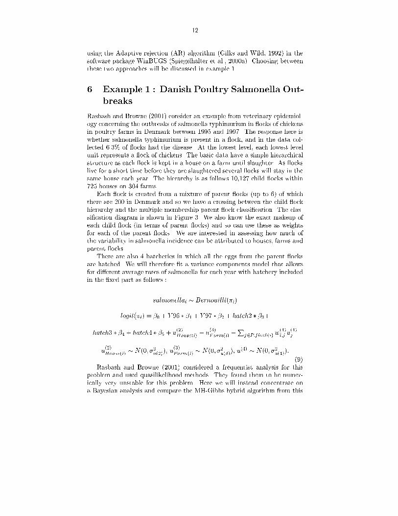
Example � � Danish Poultry Salmonella Out�breaks
Rasbash and Browne ����� consider an example from veterinary epidemiol�ogy concerning the outbreaks of salmonella typhimurium in �ocks of chickensin poultry farms in Denmark between ��� and ����� The response here iswhether salmonella typhimurium is present in a �ock� and in the data col�lected ���� of �ocks had the disease� At the lowest level� each lowest levelunit represents a �ock of chickens� The basic data have a simple hierarchicalstructure as each �ock is kept in a house on a farm until slaughter� As �ockslive for a short time before they are slaughtered several �ocks will stay in thesame house each year� The hierarchy is as follows ����� child �ocks within� houses on ��� farms�
Each �ock is created from a mixture of parent �ocks �up to �� of whichthere are �� in Denmark and so we have a crossing between the child �ockhierarchy and the multiple membership parent �ock classi�cation� The clas�si�cation diagram is shown in Figure �� We also know the exact makeup ofeach child �ock �in terms of parent �ocks� and so can use these as weightsfor each of the parent �ocks� We are interested in assessing how much ofthe variability in salmonella incidence can be attributed to houses� farms andparent �ocks�
There are also � hatcheries in which all the eggs from the parent �ocksare hatched� We will therefore �t a variance components model that allowsfor di�erent average rates of salmonella for each year with hatchery includedin the �xed part as follows �
salmonellai � Bernouilli�i�
logit�i� � �� � Y �� � �� � Y �� � �� � hatch � ���
hatch� � � � hatch� � � � u���House�i� � u
���Farm�i� �
Pj�P�flock�i� w
��i�j u
��j
u���House�i� � N��� ��u����� u
���Farm�i� � N��� ��u����� u
�� � N��� ��u����
���Rasbash and Browne ����� considered a frequentist analysis for this
problem and used quasilikelihood methods� They found them to be numer�ically very unstable for this problem� Here we will instead concentrate ona Bayesian analysis and compare the MH�Gibbs hybrid algorithm from this

��
Child Flock
House
Farm
Parent Flock
Figure �� Classi�cation diagram for the Danish poultry model�
paper �programmed in MLwiN� with the adaptive rejection �AR� method�Gilks and Wild ���� used in the WinBUGS package� To �t this model in aBayesian framework we need to include priors for the � variance parametersand the �xed e�ects� As we have no prior information we will use �di�usepriors as de�ned earlier�
The results of �tting model � using both these MCMC methods can beseen in Table �� The MCMC results for both methods were based on a runof ����� iterations after a burn�in of ������ as we used arbitrary startingvalues and so the chain took some time to converge�
From Table � we can see close agreement between the two methods� whichis to be expected as they are �tting exactly the same model� As reportedin Browne and Draper ����� for other logistic regression problems� whichmethod is preferable is a balance between the speed of the MH�Gibbs methodand the reduced Markov chain autocorrelation of the AR method� Here theMH method took hour minutes whilst WinBUGS took � hours �� minutes�Although for the �xed e�ects the expected required run lengths based on theRaftery�Lewis diagnostic �Raftery�Lewis ���� were �� times longer for theMH method� the worst mixing parameter was the between house variance�This parameter is updated via a Gibbs sampling step in each method andtherefore has similar expected run lengths�
Examining the model estimates we can see here that there are large e�ectsfor the year the chickens were born and for hatchery� There is also a large
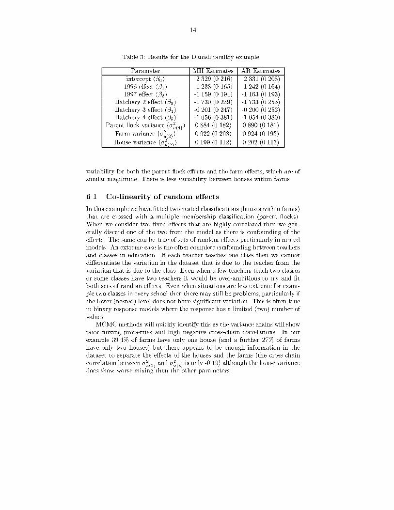
��
Table �� Results for the Danish poultry example�
Parameter MH Estimates AR Estimatesintercept ���� ���� ������ ����� ������
���� e�ect ���� ����� ����� � ���� ����������� e�ect ���� ���� � ������� ������ �������
Hatchery e�ect ���� ������ ��� �� ������ ��� �Hatchery � e�ect ��� ����� ������ ����� ��� �Hatchery � e�ect ��� ���� � ������� ���� � �������
Parent �ock variance ���u��� ����� ������ ����� �������
Farm variance ���u���� ��� ������ ���� �������
House variance ���u���� ����� ������ ��� �������
variability for both the parent �ock e�ects and the farm e�ects� which are ofsimilar magnitude� There is less variability between houses within farms�
�� Co�linearity of random e�ects
In this example we have �tted two nested classi�cations �houses within farms�that are crossed with a multiple membership classi�cation �parent �ocks��When we consider two �xed e�ects that are highly correlated then we gen�erally discard one of the two from the model as there is confounding of thee�ects� The same can be true of sets of random e�ects particularly in nestedmodels� An extreme case is the often complete confounding between teachersand classes in education� If each teacher teaches one class then we cannotdi�erentiate the variation in the dataset that is due to the teacher from thevariation that is due to the class� Even when a few teachers teach two classesor some classes have two teachers it would be over�ambitious to try and �tboth sets of random e�ects� Even when situations are less extreme for exam�ple two classes in every school then there may still be problems� particularly ifthe lower �nested� level does not have signi�cant variation� This is often truein binary response models where the response has a limited �two� number ofvalues�
MCMC methods will quickly identify this as the variance chains will showpoor mixing properties and high negative cross�chain correlations� In ourexample ����� of farms have only one house �and a further �� of farmshave only two houses� but there appears to be enough information in thedataset to separate the e�ects of the houses and the farms �the cross chaincorrelation between ��u��� and ��u��� is only ������ although the house variancedoes show worse mixing than the other parameters�

�
�� Complex random e�ects
The model described by ��� is essentially a variance components model butwe could �t a model that has complex variation at one of the higher classi��cations� To illustrate this we will modify the farm classi�cation variance toaccount for di�erent variability between years at the farm classi�cation� that
is we replace the simple farm classi�cation random e�ects� u���Farm�i� with �
sets of e�ects one for each year� Our expanded model is then as follows �
salmonellai � Bernouilli�i�
logit�i� � �� � Y �� � �� � Y �� � �� � hatch � ���
hatch� � � � hatch� � � � u���House�i� � Y � � u
���Farm�i����
Y �� � u���Farm�i��� � Y �� � u
���Farm�i��� �
Pj�P�flock�i� w
��i�j u
��j
u���House�i� � N��� ��u����� u
���Farm�i� � N�����u����� u
�� � N��� ��u����
����
The farm classi�cation variance is now a matrix and so in a Bayesianformulation we need to set a prior for this matrix� Following the example ofSpiegelhalter et al� ����� in their birats example we use a vaguely informa�tive Wishart prior with parameters� S � I� and � � �� Here I� is the �� �identity matrix� For the �xed e�ects and other variances we use the samepriors as in model ����
The parameter estimates for this extended model for both the MH andAR methods are given in Table �� Again both methods give similar estimatesas would be expected and this time the MH method takes hours �� minutesas opposed to �� hours � minutes for the AR method� The mixing propertiesof the Markov chain were similar to the last model� the MH method givingexpected run lengths generally �� times greater for �xed e�ects but againthe worst mixing parameter was the house classi�cation variance with longerexpected run length for the AR method�
It can be seen that the �xed e�ects estimates for this model are fairlysimilar to model �� It is interesting to see that all the covariances in the farmlevel variance matrix are positive� This suggests that after adjusting for otherfactors� if a farm has an incidence of salmonella in ��� then it is more likelyto have an incidence again in ���� and in ����� In fact the correspondingcorrelation estimates are ����� ���� and ���� respectively� showing that� inparticular� there is a fairly strong correlation between salmonella infection infarms in ���� and �����
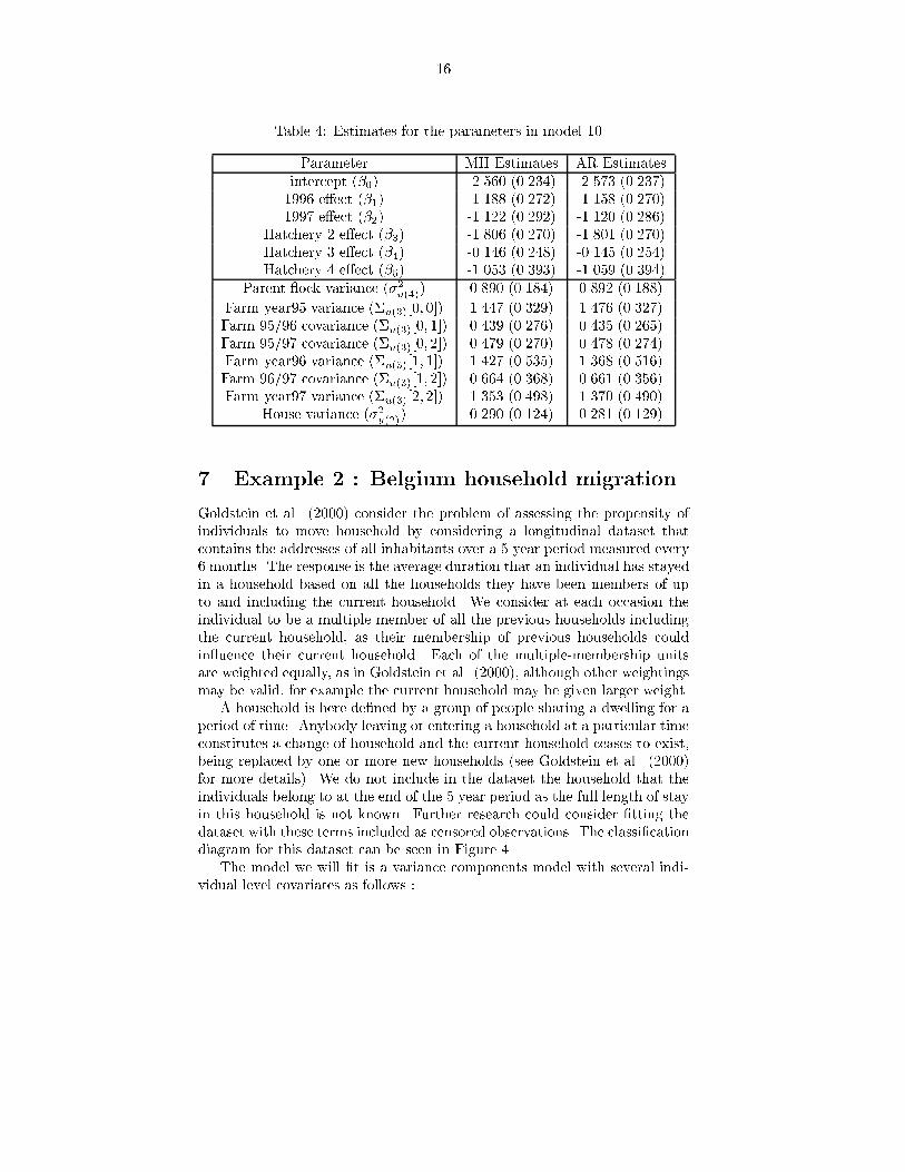
��
Table �� Estimates for the parameters in model ���
Parameter MH Estimates AR Estimatesintercept ���� �� �� ������ �� �� ������
���� e�ect ���� ������ ����� ���� � ���������� e�ect ���� ���� ����� ����� ������
Hatchery e�ect ���� ������ ������ ������ ������Hatchery � e�ect ��� ������ ������ ����� ��� ��Hatchery � e�ect ��� ���� � ������� ���� � �������
Parent �ock variance ���u��� ����� ������� ���� �������
Farm year� variance ��u������ � � ����� ������ ����� ������Farm � ��� covariance ��u������ � � ����� ������ ���� ���� �Farm � ��� covariance ��u������ � ����� ������ ����� ������Farm year�� variance ��u������ � � ���� ��� � � ����� ��� ���
Farm ����� covariance ��u������ � ����� ������� ����� ���� ��Farm year�� variance ��u����� � ��� � ������� ����� �������
House variance ���u���� ���� ������ ���� ������
� Example � � Belgium household migration
Goldstein et al� ����� consider the problem of assessing the propensity ofindividuals to move household by considering a longitudinal dataset thatcontains the addresses of all inhabitants over a year period measured every� months� The response is the average duration that an individual has stayedin a household based on all the households they have been members of upto and including the current household� We consider at each occasion theindividual to be a multiple member of all the previous households includingthe current household� as their membership of previous households couldin�uence their current household� Each of the multiple�membership unitsare weighted equally� as in Goldstein et al� ������ although other weightingsmay be valid� for example the current household may be given larger weight�
A household is here de�ned by a group of people sharing a dwelling for aperiod of time� Anybody leaving or entering a household at a particular timeconstitutes a change of household and the current household ceases to exist�being replaced by one or more new households �see Goldstein et al� �����for more details�� We do not include in the dataset the household that theindividuals belong to at the end of the year period as the full length of stayin this household is not known� Further research could consider �tting thedataset with these terms included as censored observations� The classi�cationdiagram for this dataset can be seen in Figure ��
The model we will �t is a variance components model with several indi�vidual level covariates as follows �
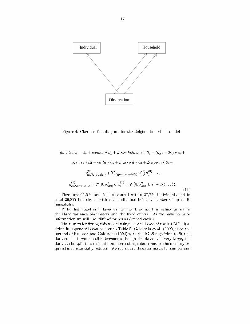
��
Observation
Individual Household
Figure �� Classi�cation diagram for the Belgium household model�
durationi � �� � gender � �� � householdsize � �� � �age� ��� � ���
spouse � � � child � � � married � �� � Belgian � ���
u���individual�i� �
Pj�household�i� w
���i�j u
���j � ei
u���individual�i� � N��� ��u����� u
���j � N��� ��u����� ei � N��� ��e��
����There are ����� occasions measured within ���� � individuals and in
total ��� households with each individual being a member of up to ��households�
To �t this model in a Bayesian framework we need to include priors forthe three variance parameters and the �xed e�ects� As we have no priorinformation we will use �di�use priors as de�ned earlier�
The results for �tting this model using a special case of the MCMC algo�rithm in appendix B can be seen in Table � Goldstein et al� ����� used themethod of Rasbash and Goldstein ������ with the IGLS algorithm to �t thisdataset� This was possible because although the dataset is very large� thedata can be split into disjoint non�intersecting subsets and so the memory re�quired is substantially reduced� We reproduce these estimates for comparison

��
Table � Results for the Charleroi population dataset�
Parameter IGLS MCMCEstimate �s�e�� Estimate �s�e��
intercept ���� ����� �������� ����� ��������gender ���� ����� ����� �� ����� � ����� ��
Size of household ���� ���� � �������� ���� �� ��������Age � �� years ���� ���� ������� ���� �������
Spouse ��� ������ �������� ������ �������Child ��� ������ �������� ������ ������ �
Is Married ���� ����� �������� ������ ��������Is Belgian national ���� ������ ����� �� ������ ����� �
Between household variance ���u���� ����� ������ ����� �������
Between individual variance ���u���� ��� ������ � ��� ������ �
Residual variance ���e� ����� ��������� ����� ���������
with the MCMC method in Table �The MCMC algorithm �in MLwiN� takes a long time initially calculating
the indexing arrays ��� minutes on a ���MHz PC�� due to the huge numbersof random e�ects but this then enables the sampler to run faster ��� iterationsa minute�� The IGLS algorithm in this example takes about � minutes periteration and needs iterations to converge�
Table shows that the results for the two methods are almost identical�This is to be expected as the variance estimates are based on large numbersof higher level units and so their distributions are fairly symmetric� From theestimates we can see that people stay longer in the same household if theyare older� if they are children or spouses rather heads of household� if theyare married or if they are Belgian nationals�
Example � � Scottish lip cancer data
The Scottish lip cancer dataset �Clayton and Kaldor ����� has been anal�ysed many times using many di�erent models that attempt to account forspatial random variation� The response variable is the observed count ofmale lip cancer in the period ��� ������ by region� for the � regions of Scot�land� Research has focused on the e�ect on sun exposure using the surrogatemeasure� percentage of the workforce working in outdoor occupations� Wecan �t a spatial model into the MMMC framework by considering the ar�eas as one classi�cation and the neighbours as another multiple membershipclassi�cation� The model is then as follows �
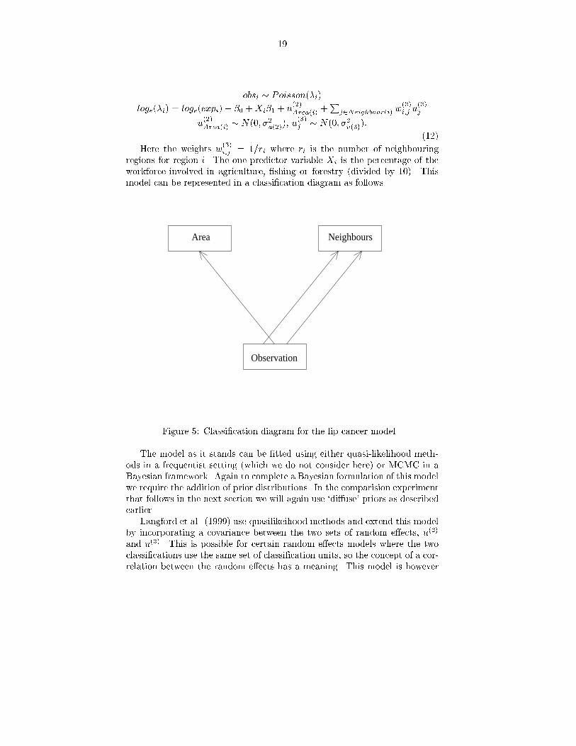
��
obsi � Poisson�i�
loge�i� � loge�expi� � �� � Xi�� � u���Area�i� �
Pj�Neighbour�i� w
���i�j u
���j
u���Area�i� � N��� ��
u����� u���j � N��� ��
u�����
���
Here the weights w���i�j � ��ri where ri is the number of neighbouring
regions for region i� The one predictor variable Xi is the percentage of theworkforce involved in agriculture� �shing or forestry �divided by ���� Thismodel can be represented in a classi�cation diagram as follows
Observation
Area Neighbours
Figure � Classi�cation diagram for the lip cancer model�
The model as it stands can be �tted using either quasi�likelihood meth�ods in a frequentist setting �which we do not consider here� or MCMC in aBayesian framework� Again to complete a Bayesian formulation of this modelwe require the addition of prior distributions� In the comparision experimentthat follows in the next section we will again use �di�use priors as describedearlier�
Langford et al� ������ use quasilikeihood methods and extend this modelby incorporating a covariance between the two sets of random e�ects� u���
and u���� This is possible for certain random e�ects models where the twoclassi�cations use the same set of classi�cation units� so the concept of a cor�relation between the random e�ects has a meaning� This model is however
�
not part of the general MMMC framework which assumes conditional inde�pendence between the random e�ects in di�erent classi�cations and so willnot be considered here�
��� Alternative spatial models to MMMC
The standard Bayesian spatial Poisson models are based on the conditionalautoregressive �CAR� prior �Besag et al� ����� that was originally used inimage analysis� These priors were used on the Scottish lip cancer dataset�Breslow and Clayton� ����� and the model can be written as follows
obsi � Poisson�i�loge�i� � loge�expi� � �� � Xi�� � ui � vi
ui � N��� ��u�� vi � N�!vi� ��v�ri��
where!vi �P
j�Neighbour�i� vj�ri�
����
Here ai is the number of neighbouring regions for region i� To �t a CARmodel using MCMC methods� again prior distributions are required and weuse the same �di�use priors as in the MMMC model� This model is infact similar to the MMMC model with two sets of random e�ects� exceptthat spatial correlation is achieved through the variance structure ratherthan through the multiple membership relationship and so the neighbourhoodrandom e�ects are not independent� It is also possible given additional data�such as the distances between neighbours� to incorporate this informationeither in the weight matrix� as in the MMMC model� or in the CAR modelframework� although this is not considered in this example�
��� Comparison of models
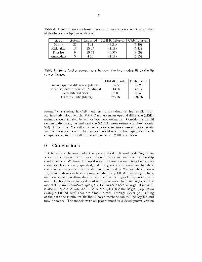
To compare the MMMC and CAR models we performed a cross validationstudy �i�e� delete jackknife� of the lip cancer dataset� For each region in turnwe set its actual deaths to be a missing value and �tted both the MMMC andCAR models to the data� At each iteration the missing value was imputedand consequently we obtained an estimate of the posterior distribution of the�unknown� observed number of cases for the region� As an MCMC method forthe CAR model is not available currently in the MLwiN package we insteadused the AR algorithm in the WinBUGS package for both models�
Both methods appeared to give reasonable interval estimates and Table �gives the results for regions where the interval estimates from one of themethods did not contain the actual number of deaths� The MMMC methodgave � � intervals that contained the true value � out of � times and theCAR method � out of � times� but further work involving cross validationneeds to be done here�
In terms of point estimates� Table � contains some additional informa�tion about the two methods� Both the mean and median estimates were �on
�
Table �� A list of regions whose intervals do not contain the actual numberof deaths for the lip cancer dataset
Area Actual Expected MMMC interval CAR intervalMoray � ���� ����� ������
Kirkcaldy �� � ��� ������ � ����Dundee � ���� ��� �� ��� ��
Annandale � ���� ������ ���� �
Table �� Some further comparisons between the two models �t to the lipcancer dataset
MMMC model CAR modelmean squared di�erence �Means� � ��� ���
mean squared di�erence �Medians� ������ � ���mean interval width ���� � �
closer estimate �Mean� �� � �� �
average� closer using the CAR model and this method also had smaller aver�age intervals� However� the MMMC models mean squared di�erence �MSD�estimates were in�ated by one or two poor estimates� Considering the �regions individually we �nd that the MMMC mean estimate is closer nearly �� of the time� We will consider a more extensive cross�validation studyand compare results with the Langford model in a further paper� along withcomparisons using the DIC �Spiegelhalter et al� ���b� criterion�
� Conclusions
In this paper we have extended the now standard multilevel modelling frame�work to encompass both crossed random e�ects and multiple membershiprandom e�ects� We have developed notation based on mappings that allowsthese models to be easily speci�ed� and have given several examples that showthe power and scope of this extended family of models� We have shown how aBayesian analysis can be easily implemented using MCMC based algorithms�and how these algorithms do not have the disadvantage of frequentist maxi�mum likelihood based methods that need large amounts of memory when themodel structure becomes complex� and the datasets become large� However itis also important to note that in some examples �like the Belgian populationexample studied here� that are almost nested� through clever partitioningof the data the maximum likelihood based methods can still be applied andmay be faster� The models were all programmed in a development version
of the MLwiN package �Rasbash et al� ���a� which will be available to theuser community in ���� More information on MLwiN is available at themultilevel modelling project website �http���multilevel�ioe�ac�uk���
�� Extensions
In the models in this paper we consider a simple variance at the lowest levelof the model� Browne et al� ����� show how to incorporate complex level� variation within the MCMC algorithm to allow for heteroscedasticity innormal response models� This extension to the simple multilevel modellingframework can easily be combined with the cross�classi�ed and multiple mem�bership models that are covered in this paper�
In the Belgian example we have omitted the censored data of the lasthousehold that individuals belong to� The data are also all left censored asit is assumed that every individual starts in their �rst household � monthsbefore the �rst data collection point� It would be useful to reanalyse thisexample while also modelling the censored data using a survival type model�This could easily be implemented in an MCMC framework by imputing thetrue data based on the censored data and a known prior distribution�
In the lip cancer example we performed some initial comparisons betweenan MMMC model that can be applied to spatial data and the standard CARspatial models� We intend to extend this comparison work while consideringBayesian formulations for the MMMC model with correlated random e�ectsas described in Langford et al� �������
Appendix A � Details of MCMC Algorithm fornormal model in section ���
For the Normal model in section �� we use a Gibbs sampling algorithm whichinvolves random draws from the following six full�conditional distributions�
Step �� Update the �xed e�ects parameter vector � from its full condi�tional distribution which is multivariate normal with dimension pf �
p�� j y� u���� u�����u�����u���� ��e � � Npf �b�� bD�� wherebD �
hPNi��
�Xi�TXi
��e� S��p
i��andb� � bD hP
i�Xi�
T di��e
� S��p �p
i�where
di � yi � Z���i u
���C��i�
�P
j�C��i�w���i�j Z
���i u
���j �
����
Step � Update the �simple classi�cation units� u���k � from their multi�
variate normal full conditional distribution with dimension p� �
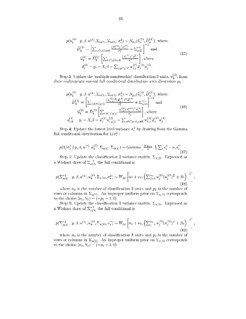
�
p�u���k j y� �� u�����u�����u���� �
�e� � Np��bu���k � bD���
k �� where
bD���k �
�Pi�C��i��k
�Z���i
�TZ���i
��e� ���
u���
���and
bu���k � bD���k
�Pi�C��i��k
�Z���i
�T d���i
��e
��where
d���i � yi �Xi� �
Pj�C��i�
w���i�j Z
���i u
���j �
�� �
Step �� Update the �multiple membership classi�cation � units� u���k � from
their multivariate normal full conditional distribution with dimension p� �
p�u���k j y� �� u�����u�����u���� �
�e� � Np��bu���k � bD���
k �� where
bD���k �
�Pi�k�C��i�
�w���
i�k���Z
���
i�TZ
���
i
��e� ���
u���
���and
bu���k � bD���k
�Pi�k�C��i�
w���
i�k�Z
���i
�Td���
i�k
��e
��where
d���i�k � yi �Xi� � Z
���i u
���C��i�
�P
j�C��i��j ��kw���i�j Z
���i u
���j �
����
Step �� Update the lowest level variance ��e by drawing from the Gammafull conditional distribution for ����e �
p�����e j y� �� u���� u
���k ��u�����u���� � Gamma
�N��e� � ��
Pi e
�i � �es
�e
�����
Step � Update the classi�cation variance matrix� �u���� Expressed as
a Wishart draw of ���u��� the full conditional is
p����u��� j y� �� u
���� u���k ��u���� �
�e � �Wp�
�n� � ���
�Pn�
j�� u���j �u
���j �T � S�
�����
����where n� is the number of classi�cation units and p� is the number of
rows or columns in �u���� An improper uniform prior on �u��� correspondsto the choice ���� S�� � ��p� � �� ���
Step �� Update the classi�cation � variance matrix� �u���� Expressed as
a Wishart draw of ���u��� the full conditional is
p����u��� j y� �� u
���� u���k ��u���� �
�e � �Wp�
�n� � ���
�Pn�
j�� u���j �u
���j �T � S�
�����
����where n� is the number of classi�cation � units and p� is the number of
rows or columns in �u���� An improper uniform prior on �u��� correspondsto the choice ���� S�� � ��p� � �� ���

�
Appendix B � Details of MCMC Algorithm forBinomial and Poisson models in section ���
The above algorithm for the general three classi�cation normal responsemodel can be easily adapted to both Binomial and Poisson response models�Here we will use univariate Metropolis updates for the �xed e�ects and setsof classi�cation and � residuals as the full conditionals do not have stan�dard forms� For ease of notation in the full conditionals that follow we de�nei � Xi� � Z
���i u
���C��i�
�P
j�C��i�w���i�j Z
���i u
���j �
Step �� Update � using univariate random walk Metropolis at time t asfollows � for l � �� � � � � pf and with ���l� signifying the beta vector withoutcomponent l �
�l�t� � ��l with probability minh��
p���l jy�u����u�������l��
p��l�t���jy�u����u�������l��
i� �l�t� �� otherwise�
���
where ��l � N��l�t� ��� ���l� and
p��l j y� u���� u���� ���l�� Q
i�� � e��i �yi �� � e�i yi�mi ���
for the logistic Binomial and
p��l j y� u���� u���� ���l��
Qi�e
�i yie�e�i ��
for the Poisson regression�
Step � Update the �simple classi�cation units� u���k � using univariate
random walk Metropolis at time t as follows � for k � �� � � � � n� and l �
�� � � � � p� and with u���k��l� signifying the u
���k vector without component l�
u���k�l��t� � u
����k�l� with probability min
���
p�u����
k�l�jy�u
����
k��l��u������ u����
p�u���
k�l��t���jy�u
���
k��l��t����u������ u����
�� u
���k�l��t� �� otherwise�
���
where u����k�l� � N�u
���k�l��t� ��� ���kl and
p�u���k�l� j y� u
���k��l�� u
���� ���u����
exp�� �� �u
���k �T���
u���u���k �
Qi�k�C��i�
�� � e��i �yi �� � e�i yi�mi���
for the logistic Binomial and
p�u���k�l� j y� u
���k��l�� u
���� ���u����
exp�� �� �u
���k �T���
u���u���k �
Qi�k�C��i�
�e�i yie�e�i
� �
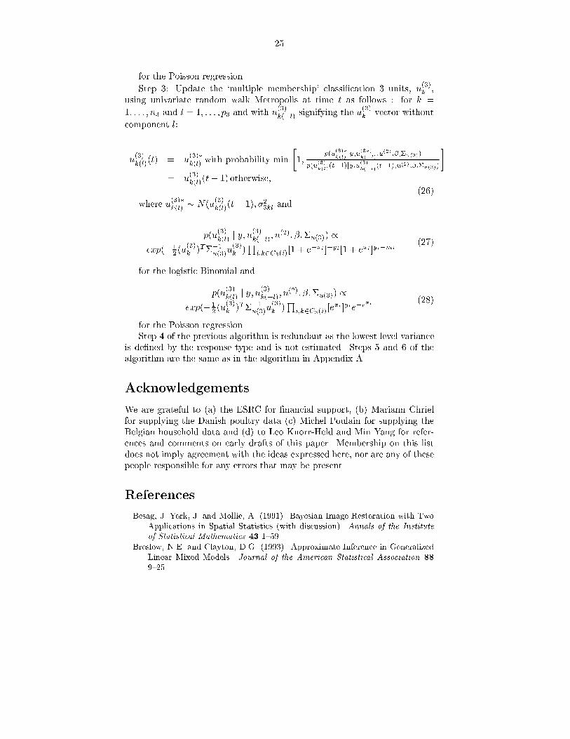
for the Poisson regression�
Step �� Update the �multiple membership classi�cation � units� u���k �
using univariate random walk Metropolis at time t as follows � for k �
�� � � � � n� and l � �� � � � � p� and with u���k��l� signifying the u
���k vector without
component l�
u���k�l��t� � u
����k�l� with probability min
���
p�u����
k�l�jy�u
����
k��l��u������ u����
p�u���
k�l��t���jy�u
���
k��l��t����u������ u����
�� u
���k�l��t� �� otherwise�
���
where u����k�l� � N�u
���k�l��t� ��� ���kl and
p�u���k�l� j y� u
���k��l�� u
���� ���u����
exp�� �� �u
���k �T���
u���u���k �
Qi�k�C��i�
�� � e��i �yi �� � e�i yi�mi���
for the logistic Binomial and
p�u���k�l� j y� u
���k��l�� u
���� ���u����
exp�� �� �u
���k �T���
u���u���k �
Qi�k�C��i�
�e�i yie�e�i
���
for the Poisson regression�Step � of the previous algorithm is redundant as the lowest level variance
is de�ned by the response type and is not estimated� Steps and � of thealgorithm are the same as in the algorithm in Appendix A�
Acknowledgements
We are grateful to �a� the ESRC for �nancial support� �b� Mariann Chrielfor supplying the Danish poultry data �c� Michel Poulain for supplying theBelgian household data and �d� to Leo Knorr�Held and Min Yang for refer�ences and comments on early drafts of this paper� Membership on this listdoes not imply agreement with the ideas expressed here� nor are any of thesepeople responsible for any errors that may be present�
References
Besag� J� York� J� and Mollie� A� ������� Bayesian Image Restoration with TwoApplications in Spatial Statistics �with discussion�� Annals of the Instituteof Statistical Mathematics �� �����
Breslow� N�E� and Clayton� D�G� ������ Approximate Inference in GeneralizedLinear Mixed Models� Journal of the American Statistical Association ��
����

�
Browne� W�J� and Draper� D� ������ Implementation and performance issuesin the Bayesian and likelihood �tting of multilevel models� ComputationalStatistics �� ��� ��
Browne� W�J� and Draper� D� ������ A comparison of Bayesian and likelihoodmethods for �tting multilevel models� Submitted for publication�
Browne� W�J�� Draper� D�� Goldstein� H�� and Rasbash� J� ������ Bayesianand likelihood methods for �tting multilevel models with complex level��variation� Computational Statistics and Data Analysis �to appear�
Bryk� A�S� and Raudenbush� S�W� ������ Hierarchical Linear Models� Applica�tions and Data Analysis Methods� London� Sage�
Bryk� A�S�� Raudenbush� S�W�� Seltzer� M� and Congdon� R� ������� An Intro�duction to HLM� Computer Program and User�s guide� Chicago� Universityof Chicago Dept� of Education�
Clayton� D�G� ������ Generalized linear mixed models� In Markov Chain MonteCarlo in Practice �eds W�R� Gilks� S� Richardson and D�J� Spiegelhalter��London� Chapman and Hall�
Clayton� D�G� and Kaldor� J� ������ Empirical Bayes Estimates of Age�StandardizedRelative Risks for Use in Disease Mapping� Biometrics �� ��������
Clayton� D�G� and Rasbash� J� ������� Estimation in large crossed random�e�ectsmodels by data augmentation� Journal of the Royal Statistics Society� SeriesA ��� �� ��
Draper� D� ������ Bayesian Hierarchical Modeling� New York� Springer�Verlag�forthcoming�
Gelfand� A�E� and Smith� A�F�M� ������� Sampling Based Approaches to Calcu�lating Marginal Densities� Journal of the American Statistical Association���� ��� ���
Gilks� W�R� and Wild� P� ������ Adaptive Rejection Sampling for Gibbs Sam�pling� Journal of the Royal Statistical Society� Series C ��� �� ��
Goldstein� H� ������� Multilevel mixed linear model analysis using iterative gen�eralised least squares� Biometrika� ��� ����
Goldstein� H� ������� Multilevel Statistical Models� Second Edition� London�Edward Arnold�
Goldstein� H� and Rasbash� J� ������� Improved approximations for multilevelmodels with binary responses� Journal of the Royal Statistical Society� SeriesA ��� �������
Goldstein� H�� Rasbash� J�� Browne� W�J�� Woodhouse� G� and Poulain� M������� Multilevel models in the study of dynamic household structures�To appear in European Journal of population
Harville� D� ������� Maximum Likelihood approaches to variance componentestimation and to related problems� Journal of the American Statistical As�sociation� �� �� ��
Hill� P�W� and Goldstein� H� ������ Multilevel modelling of educational data withcross�classi�cation and missing identi�cation of units� Journal of Educationaland Behavioral Statistics �� �������
Langford� I�H�� Leyland� A�H�� Rasbash� J�� Goldstein� H�� Day� R�J�� and McDon�ald� A�L� ������ Multilevel Modelling of Area�Based Health Data� In DiseaseMapping and Risk Assessment for Public Health �eds A� Lawson� A� Biggeri�D� Bohning� E� Lesa�re� J�F Viel and R�Bertollini�� Chichester� Wiley�

�
Lee� Y and Nelder� J� ����� Hierarchical generalized linear models� a synthesis ofgeneralized linear models� random�e�ects models� and structured dispersion�Technical report� Department of Mathematics� Imperial College� London�
Nelder� J� and Wedderburn� R� ����� Generalized linear models� Journal of theRoyal Statistical Society� Series A� � ���� �
Pan� J��X� and Thompson� R� ����� Generalized linear mixed models� An im�proved estimating procedure� COMPSTAT� Proceedings in ComputationalStatistics� ���� �edited by J�G� Bethlehem and P�G�M� van der Heijden�Physica�Verlag� ����
Rasbash� J� ������� The ML software package� London� Institute of Education�University of London�
Rasbash� J� and Goldstein� H� ���� �� E�cient analysis of mixed hierarchical andcrossed random structures using a multilevel model� Journal of BehaviouralStatistics �� �����
Rasbash� J� and Browne� W�J� ������ Non�hierarchical multilevel models� InLeyland A� and Goldstein H� �Eds� Multilevel modelling of health statisticsChichester� Wiley�
Rasbash� J�� Browne� W�J�� Goldstein� H�� Yang� M�� Plewis� I�� Healy� M� Wood�house� G�� Draper� D�� Langford� I� and Lewis� T� ����a�� A User�s Guideto MLwiN� Version ��� London� Institute of Education� University of London�
Rasbash� J�� Browne� W�J�� Healy� M� Cameron� B and Charlton� C� ����b��The MLwiN software package version ����� London� Institute of Education�University of London�
Raudenbush� S�W� ������ A crossed random e�ects model for unbalanced datawith applications in cross�sectional and longitudinal research� Journal ofEducation Statistics� �� �����
Rodriguez� G� and Goldman� N� ������� An assessment of estimation proceduresfor multilevel models with binary responses� Journal of the Royal StatisticalSociety� Series A� ��� �����
Schafer� J�L� ������� Analysis of Incomplete Multivariate Data� London� Chap�man and Hall�
Spiegelhalter� D�J�� Thomas� A�� and Best� N�G� ����a�� WINBUGS Version��� User Manual� Cambridge� Medical Research Council Biostatistics Unit�
Spiegelhalter� D�J�� Best� N�G�� and Carlin� B�P� ����b�� Bayesian deviance� thee�ective number of parameters� and the comparison of arbitrarily complexmodels� In preparation�
Tanner� M� and Wong� W� ������� The calculation of posterior distributions bydata augmentation �with discussion�� Journal of the American StatisticalAssociation �� �������