general theory of inferential models i. conditional inference

GENERAL THEORY OF INFERENTIAL MODELS I.CONDITIONAL INFERENCE

By Ryan Martin, Jing-Shiang Hwang, and Chuanhai Liu

Indiana University-Purdue University Indianapolis, Academia Sinica, andPurdue University

As applied problems have grown more complex, statisticians havebeen gradually led to reconsider the foundations of statistical in-ference. The recently proposed inferential model (IM) framework ofMartin, Zhang and Liu (2010) achieves an interesting compromise be-tween the Bayesian and frequentist ideals. Indeed, inference is basedon posterior probability-like quantities, but there are no priors andthe inferential output satisfies certain desirable long-run frequencyproperties. In this two-part series, we further develop the theory ofIMs into a general framework for statistical inference.

Here, in Part I, we build on the idea of making inference by pre-dicting unobserved auxiliary variables, focusing primarily on an inter-mediate step of conditioning, whereby the dimension of this auxiliaryvariable is reduced to a manageable size. This dimension reductionstep leads to a simpler construction of IMs having the required long-run frequency properties. We show that under suitable conditions,this dimension reduction step can be made without loss of informa-tion, and that these conditions are satisfied in a wide class of models,including those with a group invariance structure. The importantcredibility theorem of Zhang and Liu (2010) is extended to handlethe case of conditional IMs, and connections to conditional inferencein the likelihood framework are made which, in turn, allow for nu-merical approximation of the conditional posterior belief functionsusing the well-known “magic formula” of Barndorff-Nielsen (1983).The conditional IM approach is illustrated on a variety of examples,including Fisher’s problem of the Nile.

1. Introduction. R. A. Fisher’s brand of statistical inference (Fisher1973) is often viewed as some sort of middle-ground between the purelyBayesian and purely frequentist approaches. Two important examples arehis fiducial argument (Fisher 1935a; Zabell 1992) and his ideas on condi-tional inference (Fisher 1925, 1934, 1935b). As modern statistical problemshave grown more complex, contemporary statisticians have been graduallyled to reconsider the foundations of statistical inference. Perhaps influenced

AMS 2000 subject classifications: Primary 62A01; secondary 68T37, 62B05Keywords and phrases: Ancillarity, Bayes, belief functions, conditional inference, fre-

quentist, sufficiency, predictive random sets

1file: MHL-cond.tex date: August 17, 2010

2 MARTIN, HWANG, AND LIU

by ideas of Fisher, a current focus is on achieving some sort of compromisebetween the Bayesian and frequentist ideals. Case in point is the recentwork on objective Bayesian analysis with default/reference priors (Berger2006; Berger, Bernardo and Sun 2009; Ghosh, Delampady and Samanta2006). An important goal of objective Bayes analysis is to construct pri-ors for which certain posterior inferences, such as credible intervals, closelymatch that of a frequentist, so the spirit of compromise is clear; the cali-brated Bayesian analysis of Rubin (1984), Dawid (1985), and Little (2010)has similar motivations. But difficulties remain in choosing good referencepriors for high-dimensional problems so, despite these efforts, a fully satis-factory objective Bayes theory has yet to emerge. Efron (1998) predicts that(i) statistical problems in the 21st century will require new tools with goodBayesian/frequentist properties, and (ii) that “something like fiducial infer-ence” will be influential to the development of these tools. He was correcton the first part of his prediction: empirical Bayes methods, for example,have been influential in analyzing data coming from new high-throughputdevices such as microarrays (Efron 2008, 2010). The second part of Efron’sprediction remains uncertain. The goal of this series of three papers is tofurther develop the notion of inferential models—a new “something like fidu-cial inference”—into a general framework for statistical inference, partiallyvalidating the second part of Efron’s prediction.

Recently, Martin, Zhang and Liu (2010) present a modification of theDempster-Shafer theory of belief functions that has desirable Bayesian-and frequentist-like qualities in the statistical inference problem. Dempster-Shafer (DS) theory (Dempster 1966, 1967, 1968, 2008; Shafer 1976), an ex-tension of Fisher’s fiducial argument, gives a recipe for constructing a pos-terior belief function over the parameter space Θ using only the samplingmodel and observed data; in particular, no prior distribution over Θ is as-sumed or required. Although DS theory is widely used in computer scienceand engineering (Yager and Liu 2008), posterior belief functions for statisti-cal inference have yet to be widely accepted, perhaps because the numericalvalues assigned by these conventional belief functions do not, in general,have the long-run frequency properties statisticians are familiar with. Mar-tin, Zhang and Liu (2010) extend the ideas of Zhang and Liu (2010) andpropose a framework of inferential models (IMs) in which the conventionalposterior belief functions are suitably weakened so that certain long-runfrequency properties are realized. These details may be unfamiliar to somereaders (see Section 2), but that the resulting inferential method achieves abalance between Bayesian and frequentist ideals should be clear.

The empirical results in Zhang and Liu (2010) and Martin, Zhang and

file: MHL-cond.tex date: August 17, 2010

CONDITIONAL IMS 3

Liu (2010) indicate the potential of this IM framework for a wide range ofstatistical problems—even high-dimensional problems—but the ideas andmethods presented therein are somewhat ad hoc. In particular, only veryloose guidelines for constructing IMs are given. In this two-part series ofpapers, we attempt to sharpen the ideas of Zhang and Liu (2010) and Martin,Zhang and Liu (2010) to form a general theory of IMs.

Here, in Part I, we stick with the basic but fundamental idea of mak-ing probabilistic statements about the parameter of interest by predictingan unobservable auxiliary variable; see Section 2 for a review. Our focus,however, is on a preliminary step of reducing the dimension of this aux-iliary variable before attempting its prediction. We consider a dimensionreduction step based on conditioning, and develop a framework of condi-tional IMs for making inference (hypothesis tests, confidence intervals, etc)on the unknown parameter. Important connections between our frameworkand Fisher’s ideas of sufficiency and conditional inference are made in Sec-tion 3.5. After introducing the general conditional approach in Section 3.2,we use several relatively simple textbook examples in Section 3.3 to illustratethe main ideas. In Section 3.4 we extend the main theorem of Martin, Zhangand Liu (2010), showing that the desirable long-run frequency properties areattained over a “relevant subset” of the sample space. Theoretical propertiesof conditional IMs are investigated in Section 4 for a broad class of samplingmodels which are invariant under a general group of transformation, andSection 5 provides details of a conditional IM analysis for Fisher’s problemof the Nile. Some concluding remarks are made in Section 6.

2. Sampling model and statistical a-inference. In this section wedescribe the basic sampling model as well as review belief functions and theconstruction of inferential models (IMs). Some relatively simple exampleswill be considered in Section 2.4.

2.1. Sampling model and a-equation. The sampling model Pθ is a prob-ability measure on X that encodes the joint distribution of the data vectorX = (X1, . . . , Xn)′. As in Martin, Zhang and Liu (2010), we further assumethat the sampling model Pθ is defined as follows. Take U to be a more-or-lessarbitrary auxiliary space equipped with a probability measure ν. In whatfollows, we will occasionally attach the “a-” prefix to quantities/concepts re-lated to this auxiliary space; that is, we call U the a-space, ν the a-measure,and so on. Let a : U×Θ → X be a measurable function. Now take a randomdraw U ∼ ν, and choose X such that

(2.1) X = a(U, θ).



In other words, the sampling model for X given θ, is determined by the a-measure ν on U and the constraints (2.1). More formally, if we write aθ(u) =a(u, θ) for fixed θ, then the sampling model Pθ is the push-forward measurePθ = ν a−1

θ induced by the a-measure and the mapping aθ. Martin, Zhangand Liu (2010) call (2.1) the a-equation. This a-equation and its extension(see Part II) will be of critical importance to our development.

2.2. Belief functions. The primary tools to be used for a-inference arebelief functions, a generalization of probability measures, first introducedby Dempster (1967) and later formalized by Shafer (1976, 1979). The keyproperty that distinguishes belief functions from probability measures issubadditivity : if Bel : A → [0, 1] is a belief function defined on a collectionA of measurable subsets of Θ, then

Bel(A) + Bel(Ac) ≤ 1 for all A ∈ A .

For probability measures, equality obtains for all A, but not necessarily forbelief functions. The intuition is that evidence that does not support A maynot support Ac either. A related quantity is the plausibility function, definedas

Pl(A) = 1− Bel(Ac).

It follows immediately from the subadditivity property of Bel that

Bel(A) ≤ Pl(A) for all A ∈ A .

For this reason, Bel and Pl have often been referred to as lower and upperprobabilities, respectively (Dempster 1967). The plausibility will be partic-ularly useful for designing statistical procedures based on a posterior belieffunction output; see Section 2.5.

Following the classical Dempster-Shafer theory for statistical inference,Martin, Zhang and Liu (2010) construct a basic belief function Belx on Θas follows. For the general a-equation (2.1), define the set of data-parameterpairs which are consistent with the a-equation and a particular u in thea-space U; that is,

Mx(u) = {θ ∈ Θ : x = a(u, θ)}, u ∈ U.

Following Shafer (1976), we call Mx(u) a focal element indexed by u ∈ U.In general, the focal elements could be non-singletons, so Mx(U) can beviewed as a random set when U ∼ ν. The belief function is then just the


CONDITIONAL IMS 5

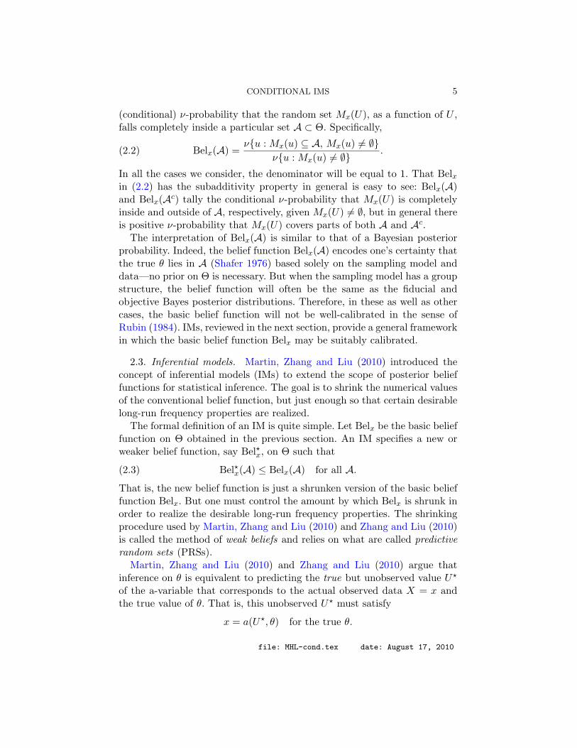
(conditional) ν-probability that the random set Mx(U), as a function of U ,falls completely inside a particular set A ⊂ Θ. Specifically,

(2.2) Belx(A) =ν{u : Mx(u) ⊆ A, Mx(u) 6= ∅}

ν{u : Mx(u) 6= ∅}.

In all the cases we consider, the denominator will be equal to 1. That Belxin (2.2) has the subadditivity property in general is easy to see: Belx(A)and Belx(Ac) tally the conditional ν-probability that Mx(U) is completelyinside and outside of A, respectively, given Mx(U) 6= ∅, but in general thereis positive ν-probability that Mx(U) covers parts of both A and Ac.

The interpretation of Belx(A) is similar to that of a Bayesian posteriorprobability. Indeed, the belief function Belx(A) encodes one’s certainty thatthe true θ lies in A (Shafer 1976) based solely on the sampling model anddata—no prior on Θ is necessary. But when the sampling model has a groupstructure, the belief function will often be the same as the fiducial andobjective Bayes posterior distributions. Therefore, in these as well as othercases, the basic belief function will not be well-calibrated in the sense ofRubin (1984). IMs, reviewed in the next section, provide a general frameworkin which the basic belief function Belx may be suitably calibrated.

2.3. Inferential models. Martin, Zhang and Liu (2010) introduced theconcept of inferential models (IMs) to extend the scope of posterior belieffunctions for statistical inference. The goal is to shrink the numerical valuesof the conventional belief function, but just enough so that certain desirablelong-run frequency properties are realized.

The formal definition of an IM is quite simple. Let Belx be the basic belieffunction on Θ obtained in the previous section. An IM specifies a new orweaker belief function, say Bel?x, on Θ such that

(2.3) Bel?x(A) ≤ Belx(A) for all A.

That is, the new belief function is just a shrunken version of the basic belieffunction Belx. But one must control the amount by which Belx is shrunk inorder to realize the desirable long-run frequency properties. The shrinkingprocedure used by Martin, Zhang and Liu (2010) and Zhang and Liu (2010)is called the method of weak beliefs and relies on what are called predictiverandom sets (PRSs).

Martin, Zhang and Liu (2010) and Zhang and Liu (2010) argue thatinference on θ is equivalent to predicting the true but unobserved value U?

of the a-variable that corresponds to the actual observed data X = x andthe true value of θ. That is, this unobserved U? must satisfy

x = a(U?, θ) for the true θ.



Both fiducial and DS inference can be understood from this viewpoint, butthey each try to predict U? with a draw U ∼ ν. But, intuitively, this isoverly optimistic since U will, in general, miss U? with ν-probability 1. Themethod of weak beliefs relaxes this assumption and instead tries to hit thetarget U? with a random set S(U) ⊇ {U}, where U ∼ ν. The set S(U) iscalled a predictive random set (PRS). Some simple examples of PRSs canbe found in Section 2.4.

For a given set-valued map S, define the enlarged focal elements

(2.4) Mx(u;S) =⋃

u′∈S(u)

{θ : x = a(u′, θ)}, u ∈ U.

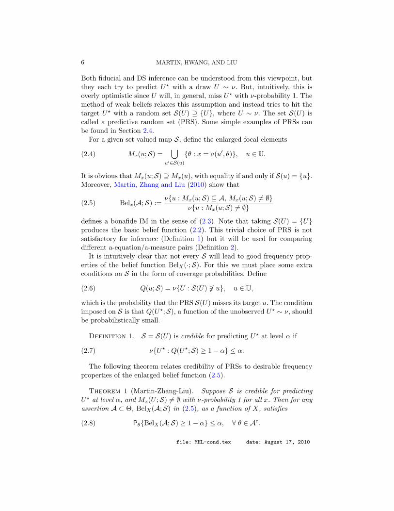
It is obvious that Mx(u;S) ⊇ Mx(u), with equality if and only if S(u) = {u}.Moreover, Martin, Zhang and Liu (2010) show that

(2.5) Belx(A;S) :=ν{u : Mx(u;S) ⊆ A, Mx(u;S) 6= ∅}

ν{u : Mx(u;S) 6= ∅}

defines a bonafide IM in the sense of (2.3). Note that taking S(U) = {U}produces the basic belief function (2.2). This trivial choice of PRS is notsatisfactory for inference (Definition 1) but it will be used for comparingdifferent a-equation/a-measure pairs (Definition 2).

It is intuitively clear that not every S will lead to good frequency prop-erties of the belief function BelX(·;S). For this we must place some extraconditions on S in the form of coverage probabilities. Define

(2.6) Q(u;S) = ν{U : S(U) 63 u}, u ∈ U,

which is the probability that the PRS S(U) misses its target u. The conditionimposed on S is that Q(U?;S), a function of the unobserved U? ∼ ν, shouldbe probabilistically small.

Definition 1. S = S(U) is credible for predicting U? at level α if

(2.7) ν{U? : Q(U?;S) ≥ 1− α} ≤ α.

The following theorem relates credibility of PRSs to desirable frequencyproperties of the enlarged belief function (2.5).

Theorem 1 (Martin-Zhang-Liu). Suppose S is credible for predictingU? at level α, and Mx(U ;S) 6= ∅ with ν-probability 1 for all x. Then for anyassertion A ⊂ Θ, BelX(A;S) in (2.5), as a function of X, satisfies

(2.8) Pθ{BelX(A;S) ≥ 1− α} ≤ α, ∀ θ ∈ Ac.


CONDITIONAL IMS 7

Therefore, IMs formed via the method of weak beliefs with credible PRSswill have the desired long-run frequency properties. The next section givessome simple examples, and Section 2.5 will show how Theorem 1 relatesto the inference problem. We refer to Ermini Leaf and Liu (2010) for dis-cussion on the case when the fundamental condition “Mx(U ;S) 6= ∅ withν-probability 1 for all x” does not hold.

At this point we should emphasize that the IM approach is substantiallydifferent from the DS and fiducial theories. While belief functions are used tomake inference, we do not adopt the fundamental operation of DS, namelyDempster’s rule of combination (Shafer 1976, Ch. 3), and therefore we avoidthe potential difficulties it entails (Ermini Leaf, Hui and Liu 2009; Wal-ley 1987). Moreover, since the belief functions we use for inference are notprobability measures, and we do not operate on them as if they were, ourconclusions cannot coincide with those resulting from a fiducial (or Bayesian)analysis. There are similarities, however, to the imprecise prior Bayes ap-proach (Walley 1996) and the robust Bayes approach (Berger 1984). Butperhaps the most important difference is our focus on long-run frequencyproperties—DS and fiducial are void of such frequentist concerns.

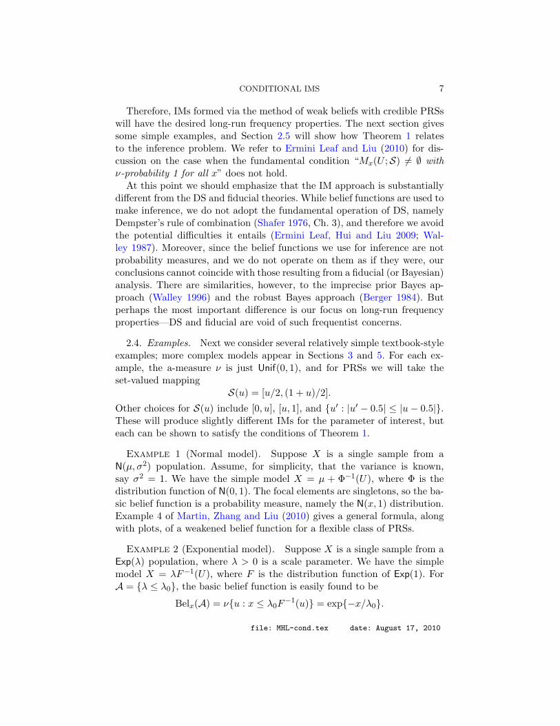
2.4. Examples. Next we consider several relatively simple textbook-styleexamples; more complex models appear in Sections 3 and 5. For each ex-ample, the a-measure ν is just Unif(0, 1), and for PRSs we will take theset-valued mapping

S(u) = [u/2, (1 + u)/2].

Other choices for S(u) include [0, u], [u, 1], and {u′ : |u′ − 0.5| ≤ |u− 0.5|}.These will produce slightly different IMs for the parameter of interest, buteach can be shown to satisfy the conditions of Theorem 1.

Example 1 (Normal model). Suppose X is a single sample from aN(µ, σ2) population. Assume, for simplicity, that the variance is known,say σ2 = 1. We have the simple model X = µ + Φ−1(U), where Φ is thedistribution function of N(0, 1). The focal elements are singletons, so the ba-sic belief function is a probability measure, namely the N(x, 1) distribution.Example 4 of Martin, Zhang and Liu (2010) gives a general formula, alongwith plots, of a weakened belief function for a flexible class of PRSs.

Example 2 (Exponential model). Suppose X is a single sample from aExp(λ) population, where λ > 0 is a scale parameter. We have the simplemodel X = λF−1(U), where F is the distribution function of Exp(1). ForA = {λ ≤ λ0}, the basic belief function is easily found to be

Belx(A) = ν{u : x ≤ λ0F−1(u)} = exp{−x/λ0}.



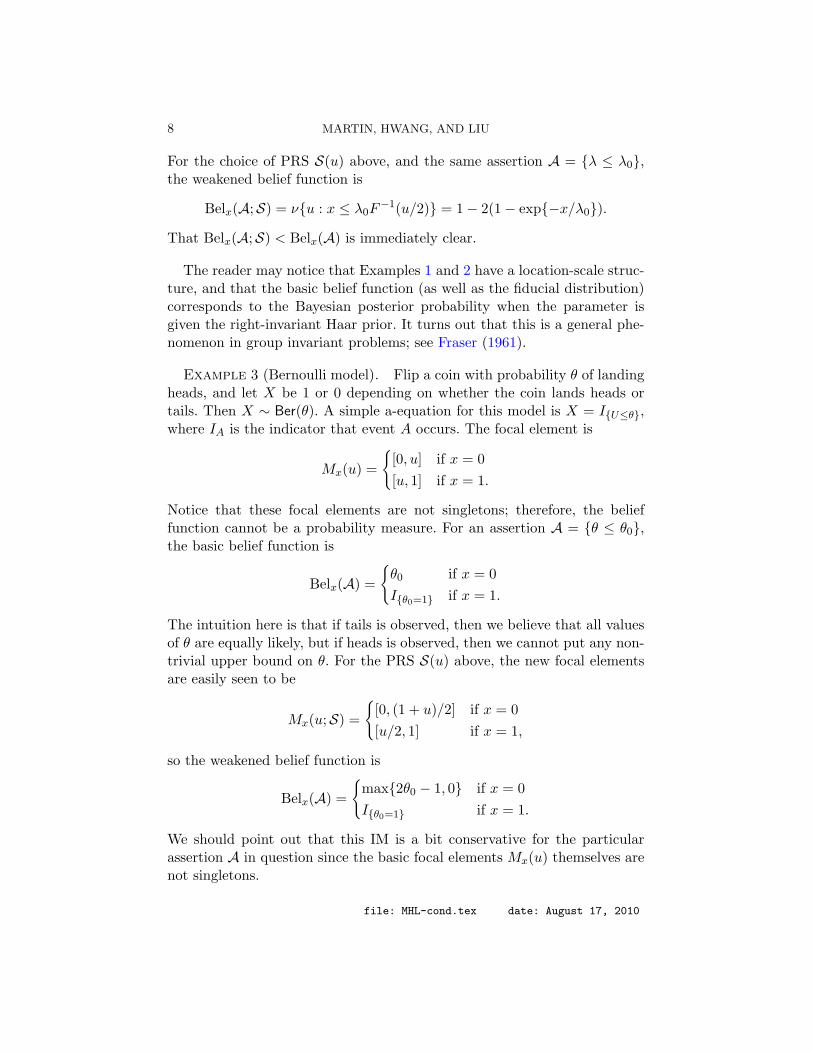
For the choice of PRS S(u) above, and the same assertion A = {λ ≤ λ0},the weakened belief function is

Belx(A;S) = ν{u : x ≤ λ0F−1(u/2)} = 1− 2(1− exp{−x/λ0}).

That Belx(A;S) < Belx(A) is immediately clear.

The reader may notice that Examples 1 and 2 have a location-scale struc-ture, and that the basic belief function (as well as the fiducial distribution)corresponds to the Bayesian posterior probability when the parameter isgiven the right-invariant Haar prior. It turns out that this is a general phe-nomenon in group invariant problems; see Fraser (1961).

Example 3 (Bernoulli model). Flip a coin with probability θ of landingheads, and let X be 1 or 0 depending on whether the coin lands heads ortails. Then X ∼ Ber(θ). A simple a-equation for this model is X = I{U≤θ},where IA is the indicator that event A occurs. The focal element is

Mx(u) =

{[0, u] if x = 0[u, 1] if x = 1.

Notice that these focal elements are not singletons; therefore, the belieffunction cannot be a probability measure. For an assertion A = {θ ≤ θ0},the basic belief function is

Belx(A) =

{θ0 if x = 0I{θ0=1} if x = 1.

The intuition here is that if tails is observed, then we believe that all valuesof θ are equally likely, but if heads is observed, then we cannot put any non-trivial upper bound on θ. For the PRS S(u) above, the new focal elementsare easily seen to be

Mx(u;S) =

{[0, (1 + u)/2] if x = 0[u/2, 1] if x = 1,

so the weakened belief function is

Belx(A) =

{max{2θ0 − 1, 0} if x = 0I{θ0=1} if x = 1.

We should point out that this IM is a bit conservative for the particularassertion A in question since the basic focal elements Mx(u) themselves arenot singletons.


CONDITIONAL IMS 9

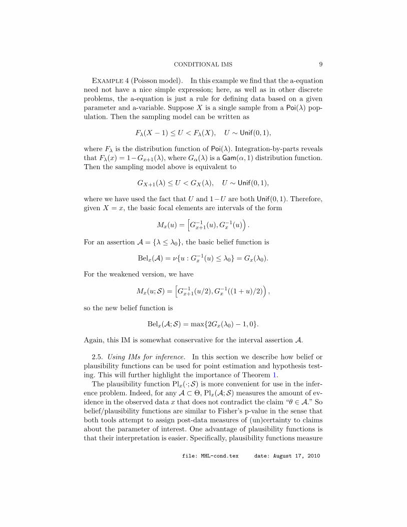
Example 4 (Poisson model). In this example we find that the a-equationneed not have a nice simple expression; here, as well as in other discreteproblems, the a-equation is just a rule for defining data based on a givenparameter and a-variable. Suppose X is a single sample from a Poi(λ) pop-ulation. Then the sampling model can be written as

Fλ(X − 1) ≤ U < Fλ(X), U ∼ Unif(0, 1),

where Fλ is the distribution function of Poi(λ). Integration-by-parts revealsthat Fλ(x) = 1−Gx+1(λ), where Gα(λ) is a Gam(α, 1) distribution function.Then the sampling model above is equivalent to

GX+1(λ) ≤ U < GX(λ), U ∼ Unif(0, 1),

where we have used the fact that U and 1−U are both Unif(0, 1). Therefore,given X = x, the basic focal elements are intervals of the form

Mx(u) =[G−1

x+1(u), G−1x (u)

).

For an assertion A = {λ ≤ λ0}, the basic belief function is

Belx(A) = ν{u : G−1x (u) ≤ λ0} = Gx(λ0).

For the weakened version, we have

Mx(u;S) =[G−1

x+1(u/2), G−1x ((1 + u)/2)

),

so the new belief function is

Belx(A;S) = max{2Gx(λ0)− 1, 0}.

Again, this IM is somewhat conservative for the interval assertion A.

2.5. Using IMs for inference. In this section we describe how belief orplausibility functions can be used for point estimation and hypothesis test-ing. This will further highlight the importance of Theorem 1.

The plausibility function Plx(·;S) is more convenient for use in the infer-ence problem. Indeed, for any A ⊂ Θ, Plx(A;S) measures the amount of ev-idence in the observed data x that does not contradict the claim “θ ∈ A.” Sobelief/plausibility functions are similar to Fisher’s p-value in the sense thatboth tools attempt to assign post-data measures of (un)certainty to claimsabout the parameter of interest. One advantage of plausibility functions isthat their interpretation is easier. Specifically, plausibility functions measure



one’s uncertainty about the claim “θ ∈ A” given data, while p-values mea-sure the probability of an observed event given the claim is true—reasoningabout θ is direct with plausibility but somehow indirect with p-values.

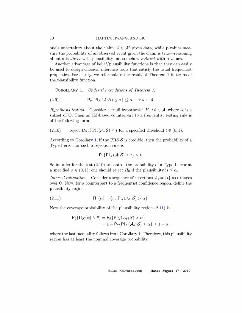
Another advantage of belief/plausibility functions is that they can easilybe used to design classical inference tools that satisfy the usual frequentistproperties. For clarity, we reformulate the result of Theorem 1 in terms ofthe plausibility function.

Corollary 1. Under the conditions of Theorem 1,

(2.9) Pθ{PlX(A;S) ≤ α} ≤ α, ∀ θ ∈ A.

Hypothesis testing. Consider a “null hypothesis” H0 : θ ∈ A, where A is asubset of Θ. Then an IM-based counterpart to a frequentist testing rule isof the following form:

(2.10) reject H0 if Plx(A;S) ≤ t for a specified threshold t ∈ (0, 1).

According to Corollary 1, if the PRS S is credible, then the probability of aType I error for such a rejection rule is

Pθ{PlX(A;S) ≤ t} ≤ t.

So in order for the test (2.10) to control the probability of a Type I error ata specified α ∈ (0, 1), one should reject H0 if the plausibility is ≤ α.

Interval estimation. Consider a sequence of assertions At = {t} as t rangesover Θ. Now, for a counterpart to a frequentist confidence region, define theplausibility region

(2.11) Πx(α) = {t : Plx(At;S) > α}.

Now the coverage probability of the plausibility region (2.11) is

Pθ{ΠX(α) 3 θ} = Pθ{PlX(Aθ;S) > α}= 1− Pθ{PlX(Aθ;S) ≤ α} ≥ 1− α,

where the last inequality follows from Corollary 1. Therefore, this plausibilityregion has at least the nominal coverage probability.


CONDITIONAL IMS 11

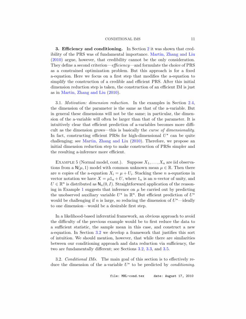
3. Efficiency and conditioning. In Section 2 it was shown that cred-ibility of the PRS was of fundamental importance. Martin, Zhang and Liu(2010) argue, however, that credibility cannot be the only consideration.They define a second criterion—efficiency—and formulate the choice of PRSas a constrained optimization problem. But this approach is for a fixeda-equation. Here we focus on a first step that modifies the a-equation tosimplify the construction of a credible and efficient PRS. After this initialdimension reduction step is taken, the construction of an efficient IM is justas in Martin, Zhang and Liu (2010).

3.1. Motivation: dimension reduction. In the examples in Section 2.4,the dimension of the parameter is the same as that of the a-variable. Butin general these dimensions will not be the same; in particular, the dimen-sion of the a-variable will often be larger than that of the parameter. It isintuitively clear that efficient prediction of a-variables becomes more diffi-cult as the dimension grows—this is basically the curse of dimensionality.In fact, constructing efficient PRSs for high-dimensional U? can be quitechallenging; see Martin, Zhang and Liu (2010). Therefore, we propose aninitial dimension reduction step to make construction of PRSs simpler andthe resulting a-inference more efficient.

Example 5 (Normal model, cont.). Suppose X1, . . . , Xn are iid observa-tions from a N(µ, 1) model with common unknown mean µ ∈ R. Then thereare n copies of the a-equation Xi = µ + Ui. Stacking these n a-equations invector notation we have X = µ1n +U , where 1n is an n-vector of unity, andU ∈ Rn is distributed as Nn(0, I). Straightforward application of the reason-ing in Example 1 suggests that inference on µ be carried out by predictingthe unobserved auxiliary variable U? in Rn. But efficient prediction of U?

would be challenging if n is large, so reducing the dimension of U?—ideallyto one dimension—would be a desirable first step.

In a likelihood-based inferential framework, an obvious approach to avoidthe difficulty of the previous example would be to first reduce the data toa sufficient statistic, the sample mean in this case, and construct a newa-equation. In Section 3.2 we develop a framework that justifies this sortof intuition. We should mention, however, that while there are similaritiesbetween our conditioning approach and data reduction via sufficiency, thetwo are fundamentally different; see Sections 3.2, 3.3, and 3.5.

3.2. Conditional IMs. The main goal of this section is to effectively re-duce the dimension of the a-variable U? to be predicted by conditioning.



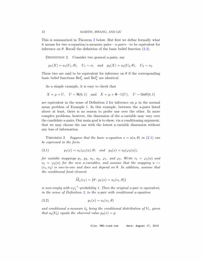
This is summarized in Theorem 2 below. But first we define formally whatit means for two a-equation/a-measure pairs—a-pairs—to be equivalent forinference on θ. Recall the definition of the basic belief function (2.2).

Definition 2. Consider two general a-pairs, say

p1(X) = a1(U1, θ), U1 ∼ ν1 and p2(X) = a2(U2, θ), U2 ∼ ν2.

These two are said to be equivalent for inference on θ if the correspondingbasic belief functions Bel1x and Bel2x are identical.

As a simple example, it is easy to check that

X = µ + U, U ∼ N(0, 1) and X = µ + Φ−1(U), U ∼ Unif(0, 1)

are equivalent in the sense of Definition 2 for inference on µ in the normalmean problem of Example 1. In this example, between the a-pairs listedabove at least, there is no reason to prefer one over the other. In morecomplex problems, however, the dimension of the a-variable may vary overthe candidate a-pairs. Our main goal is to show, via a conditioning argument,that we may choose the one with the lowest a-variable dimension withoutany loss of information.

Theorem 2. Suppose that the basic a-equation x = a(u, θ) in (2.1) canbe expressed in the form

(3.1) p1(x) = a1(ϕ1(u), θ) and p2(x) = a2(ϕ2(u)),

for suitable mappings p1, p2, a1, a2, ϕ1, and ϕ2. Write v1 = ϕ1(u) andv2 = ϕ2(u) for the new a-variables, and assume that the mapping u 7→(v1, v2) is one-to-one and does not depend on θ. In addition, assume thatthe conditional focal element

Mx(v1) = {θ : p1(x) = a1(v1, θ)}

is non-empty with νϕ−11 -probability 1. Then the original a-pair is equivalent,

in the sense of Definition 2, to the a-pair with conditional a-equation

(3.2) p1(x) = a1(v1, θ)

and conditional a-measure νp being the conditional distribution of V1, giventhat a2(V2) equals the observed value p2(x) = p.


CONDITIONAL IMS 13

Proof. The basic a-equation for the original a-pair is

Belx(A) =ν{u : Mx(u) ⊆ A, Mx(u) 6= ∅}

ν{u : Mx(u) 6= ∅}.

The assumption that the conditional focal element is non-empty implies thatthe belief function corresponding to the conditional a-pair is

Belx(A) = νp{v : Mx(v) ⊆ A} =ν{u : Mx(u) ⊆ A, a2(ϕ2(u)) = p}

ν{u : a2(ϕ2(u)) = p},

where p is the observed value p2(x). It is easy to check that the numeratorof Belx(A) is

ν{u : Mx(ϕ1(u)) ⊆ A, Mx(ϕ1(u)) 6= ∅, a2(ϕ2(u)) = p},

and since Mx(ϕ1(u)) 6= ∅ with νϕ−11 -probability 1, this reduces to

ν{u : Mx(ϕ1(u)) ⊆ A, a2(ϕ2(u)) = p}.

Likewise, the denominator of Belx(A) is simply ν{u : a2(ϕ2(u)) = p}. Takingthe ratio we get exactly Belx(A), which proves the claim.

Remark 1. The dimension reduction will be achieved by conditioningsince, generally, ϕ1(u) will be of much lower dimension than u itself; infact, ϕ1(u) will frequently be a “sufficient statistic” type of quantity, so itsdimension will be the same as θ rather than x. See Section 3.5 below.

The significance of Theorem 2 is that we obtain a new conditional a-equation (3.2) which, together with a conditional a-measure νp, for p =p2(x), can be used to construct a conditional IM along the lines in Sec-tion 2.3. That is, first specify a PRS S = S(V ) for predicting the unobserveda-variable V ? = ϕ1(U?), and define the conditional focal elements

(3.3) Mx(v;S) =⋃

v′∈S(v)

{θ : p1(x) = a1(v′, θ)}.

Then the corresponding belief function is given by

(3.4) Belx(A;S) = νp{v : Mx(v;S) ⊆ A}, A ⊆ Θ.

Then this belief function may be used, as in Section 2.5, to make inferenceon the unknown parameter θ. We revisit our examples in Section 3.3.



The very same credibility condition (Definition 1) can be considered and,in the case where νp is independent of x, the desirable frequency propertiesfor Belx(A;S) in (3.4) follow immediately from Theorem 1. Surprisingly, νp

is indeed independent of x in a number of important examples. But moregenerally, we would like to extend the notion of credibility and the result ofTheorem 1 to the case where the conditional a-measure νp indeed dependson the observed data x. This is the topic of Section 3.4 below.

3.3. Examples. Here we revisit those examples presented in Section 2.4to demonstrate the dimension reduction technique in Theorem 2.

Example 6 (Normal model, cont.). Suppose X1, . . . , Xn is an iid samplefrom a N(µ, σ2) population. If σ2 = 1 is known, then the basic a-equationcan be written as

X = µ + U, and Xi −X = Ui − U, i = 1, . . . , n.

For an independent sample U1, . . . , Un from N(0, 1), the sample mean U isindependent of Ui−U , i = 1, . . . , n, and distributed as N(0, n−1). Therefore,there is no need to predict the entire n-vector of unobserved a-variables; IMscan be constructed for inference on µ based on predicting a single a-variablewith a priori distribution N(0, n−1). More generally, for inference on (µ, σ2),the basic a-equation reduces to

{X = µ + U, s2(X) = σ2s2(U)} andXi −X

s(X)=

Ui − U

s(U),

where s2(x) = 1n−1

∑ni=1(xi − x)2 denotes the sample variance. The vector

of “z-scores” on the far-right of the previous display is known as the sampleconfiguration, and is ancillary (maximal invariant) in general location-scaleproblems. Since U and s2(U) are independent, IMs for (µ, σ2) can be builtbased on predicting V ? = (U?

, s2(U?)) using draws from the respectivemarginal distributions. The problem of, say, inference on µ alone when bothµ and σ2 are unknown is the topic of Part II of the series.

Example 7 (Exponential model, cont.). For an iid sample X1, . . . , Xn

from an Exp(λ) population, the basic a-equation can be rewritten as

T (X) = λT (U), andXi

T (X)=

Ui

T (U), i = 1, . . . , n,

where T (x) =∑n

i=1 xi is the sample total. The general result of Fraser (1966)shows that T (U) and the vector {Ui/T (U) : i = 1, . . . , n} are independent,


CONDITIONAL IMS 15

so an IM for inference on λ can be built based on predicting V ? = T (U?)with draws from its marginal distribution Gam(n, 1).

Example 8 (Bernoulli model, cont.). Suppose X1, . . . , Xn is an iid sam-ple from a Ber(θ) population. An obvious extension of the model in Exam-ple 3 is to take Xi = I{Ui≤θ}, where U1, . . . , Un are iid Unif(0, 1). It turns out,however, that the conditioning approach does not easily apply to the modelin this form. Here we consider an alternative formulation of the samplingmodel that leads to a very simple conditioning argument.

• Sample T , the total number of successes, by drawing U0 ∼ Unif(0, 1)and defining T such that

(3.5) Fn,θ(T ) ≤ U0 < Fn,θ(T + 1),

where Fn,θ(t) denotes the distribution function of Bin(n, θ).• Given T , randomly allocate the T successes and n− T failures among

the n trials. That is, randomly sample (U1, . . . , Un) from the subset of{0, 1}n consisting of exactly T ones, and set Xi = Ui, i = 1, . . . , n.

We have defined the sampling model so that the decomposition (3.1) is ex-plicit: the first step involves the parameter θ and a lower-dimensional sum-mary of the data T and a-variable U0, and the second is void of θ. There-fore, according to Theorem 2, we may consider the conditional a-equation(3.5), and it is easy to verify (via Bayes theorem) that the conditional a-measure—the distribution of U0 given (U1, . . . , Un)—is still Unif(0, 1). There-fore, a-inference on θ can proceed by predicting the unobserved U?

0 in theconditional a-equation (3.5). Note that this is exactly the result obtained byZhang and Liu (2010) when only a single T ∼ Bin(n, θ) is observed.

Example 9 (Poisson model, cont.). Suppose X1, . . . , Xn are indepen-dent observations from a Poi(λ) population. We follow the approach de-scribed in Example 8 to construct a sampling model that leads to a simpleconditioning argument.

• Sample T , the sample total, by drawing U0 ∼ Unif(0, 1) and definingT such that

(3.6) Fnλ(T ) ≤ U0 < Fnλ(T + 1),

where Fnλ(t) is the distribution function of Poi(nλ).• Randomly allocate portions of the total to the observations X1, . . . , Xn.

That is, sample (U1, . . . , Un) from a Mult(T ;n−11n) distribution andset Xi = Ui, i = 1, . . . , n.



Again, like in Example 8, the decomposition (3.1) of the sampling model intotwo components is made explicit. By Theorem 2 we may drop the secondpart, which does not involve λ, and consider the conditional a-equation(3.6). Similarly, it is easy to check that the conditional a-measure is simplyUnif(0, 1). Therefore, inference on λ can be carried out by predicting theunobserved U?

0 in the conditional a-equation (3.6).

The first two examples describe models which have a location and scalestructure, respectively. (Example 8 has a similar, but less obvious, typeof symmetry.) We show in Section 4.2 that Theorem 2 can be applied inproblems that have a more general group transformation structure.

Remark 2. The reader will have noticed that in each of the four exam-ples presented above, the dimension reduction corresponds to that obtainedby working with the data summarized by a sufficient statistic. However,the decomposition (3.1) is not unique, and the choice to use the famil-iar sufficient statistics is simply for convenience. For example, in Exam-ple 6, for inference on µ based on X1, . . . , Xn iid N(µ, 1), rather than usingthe conditional a-equation X = µ + U , we could have equivalently usedX1 = µ + U1 but with conditional a-measure being the distribution of U1

given {Ui − U1 : i = 2, . . . , n}. By choosing the average U we can make useof the well-known facts that U has a normal distribution and is independentof the residuals {Ui−U : i = 1, . . . , n}. The point is that data reduction viasufficiency singles out only an important special case of the decomposition(3.1) used to construct a conditional IM. See Section 3.5.

3.4. Conditional credibility. The goal of this section is to extend thenotion of credibility and the results of Theorem 1 to the case where theconditional a-measure νp depends on x through p = p2(x).

Let S be a set-valued mapping and, following the development in Sec-tion 2.3, define the map

Qp(v;S) = νp{V : S(V ) 63 v}.

This is just like the non-coverage probability in (2.6) but evaluated underthe conditional distribution νp for V . Analogous to Definition 1 we defineconditional credibility as follows.

Definition 3. A PRS S = S(V ) for predicting V ? is conditionallycredible at level α given p2(X) = p, if

(3.7) νp{V ? : Qp(V ?;S) ≥ 1− α} ≤ α.


CONDITIONAL IMS 17

For the focal elements Mx(v;S) in (3.3) and the corresponding belieffunction Belx(·;S), we have a conditional version of Theorem 1.

Theorem 3. Suppose S is conditionally credible for predicting V ? atlevel α, given p2(X) = p, and that Mx(V ;S) 6= ∅ with νp-probability 1 forall x such that p2(x) = p. Then for any assertion A ⊂ Θ, BelX(A;S) in(3.4), as a function of X, satisfies

(3.8) Pθ{BelX(A;S) ≥ 1− α | p2(X) = p} ≤ α, ∀ θ ∈ Ac.

Proof. The proof follows that of Theorem 3.1 in Zhang and Liu (2010).Let θ denote the true value of the parameter, and assume θ ∈ Ac. Then

Belx(A;S) ≤ Belx({θ}c;S)

= νp{v : Mx(v;S) 63 θ} = Qp(V ?;S)

for each x satisfying p2(x) = p. Therefore, Belx(A;S) ≥ 1 − α impliesQp(V ?;S) ≥ 1 − α and, consequently, the conditional probability of theformer can be no more than that of the latter. That is,

Pθ{BelX(A;S) ≥ 1− α | p2(X) = p} ≤ νp{V ? : Qp(V ?;S) ≥ 1− α},

and the result follows from the conditional credibility of S.

Corollary 2 below shows that under slightly stronger conditions the thelong-run frequency property (3.8) holds unconditionally ; the proof followsimmediately from the law of total probability.

Corollary 2. Suppose that the conditions of Theorem 3 hold for almostall p. Then (3.8) holds unconditionally, i.e.,

Pθ{BelX(A;S) ≥ 1− α} ≤ α, ∀ θ ∈ Ac.

3.5. Relations to sufficiency and classical conditional inference. Fisher’stheory of sufficiency beautifully describes how the observed data can bereduced in such a way that no information about the parameter of interestθ is lost. In cases where the dimension reduction via sufficiency alone isunsatisfactory—i.e., the dimension of the sufficient statistic is greater thanthat of the parameter—there is an equally beautiful theory of conditionalinference also due to Fisher but later built upon by others; see Reid (1995),Fraser (2004), and Ghosh, Reid and Fraser (2010) for reviews. We havealready seen a number of instances where familiar things like sufficiency,



ancillarity, and conditional inference have appeared in the new approach.But while there are some similarities, there are also a number of importantdifferences which we mention here.

(i) Fisherian sufficiency requires a likelihood function to define and justifythe data reduction. There is no likelihood function in the proposed frame-work, so a direct reduction of the observed data cannot be justified. However,we have a-variables with valid distributions which we are allowed to manip-ulate more-or-less as we please, and for certain (convenient) manipulationsof these a-variables, the familar data reduction via sufficiency emerges.

(ii) The proposed approach to dimension reduction is, in some sense, moregeneral than that of sufficiency. The key feature is the conditional a-measureattached to the decomposition (3.1). In the proposed framework, almost anychoice of decomposition is valid, and we see immediately the effect of ourchoice: a “bad” choice may have a complicated conditional a-measure, whilea “good” choice might be much easier to work with. In other words, theconditional a-measures play the role of assigning a preference ordering tothe various choices of decompositions (3.1).

(iii) In problems where the reduction via sufficiency is unsatisfactory (i.e.,when the minimal sufficient statistic has dimension greater than that of theparameter), the classical approach is to find a suitable ancillary statisticto condition on. A number of well-known examples (see Ghosh, Reid andFraser 2010) suggest that this task can be difficult in general. In the proposedsystem, the choice of decomposition (3.1) is not unique, but the procedureis basically automatic for each fixed choice.

(iv) Although they contain no information about the parameter of inter-est, ancillary statistics are important for conditional inference in the classicalsense as they identify a relevant subset of the sample space to condition on.It turns out that there are actually two notions of “relevant subsets” in theproposed framework. The first is in the conditional a-measure: building anIM based on the conditional a-measure effectively restricts the distributionof the a-variable to a lower-dimensional subspace defined by the observedvalue of a2(ϕ2(U)). The second is in the conditional credibility theorem: thelong-run frequency properties of the conditional IM are evaluated on thesubset of the sample space defined by the observed value of p2(X).

4. Theory for group transformation models. In this section wederive some general properties of conditional IMs for a fairly broad class ofmodels which are invariant under a suitable group of transformations. Forthe most part, our notation and terminology matches that of Eaton (1989).The analysis is different from, but shares some similarities with Fraser’s


CONDITIONAL IMS 19

work on fiducial/structural inference in group invariant problems.

4.1. Group transformation models. Consider a special case where Pθ isinvariant under a group G of transformations g mapping X onto itself. Thatis, there is a corresponding group G of transformations mapping Θ onto itselfsuch that if X ∼ Pθ and g ∈ G , then gX ∼ Pgθ for a suitable g ∈ G . Heregx denotes the image of x under g. A number of popular models fit into thisframework: location-scale data (e.g., normal, Student-t, gamma), directionaldata (e.g., Fisher-von Mises), and various multivariate/matrix-valued data(e.g., Wishart). Next we give some notation and definitions.

Suppose that G is transitive; i.e., for any pair θ1, θ2 ∈ Θ there exists g ∈ Gsuch that θ1 = gθ2. Choose an arbitrary reference point θ0 ∈ Θ. Then themodel X ∼ Pθ may be written in a-equation form as

(4.1) X = gU,

where U ∼ ν ≡ Pθ0 , and g is such that the corresponding g produces θ = gθ0.For a point x ∈ X, the orbit Ox of x with respect to G is defined as

Ox = {gx : g ∈ G } ⊆ X;

that is, Ox is all possible images of x under G . If G is transitive, thenOx = X. A function f : X → X is said to be invariant if it is constant onorbits; i.e., if f(gx) = f(x) for all x and all g. A function f is a maximalinvariant if f(x) = f(y) implies y = gx for some g ∈ G . A related concept isequivariance. A function t : X → Θ is equivariant if t(gx) = g t(x). Roughlyspeaking, an equivariant function preserves orbits in the sense that gx ∈ Xis mapped by t to a point on the orbit of t(x) ∈ Θ.

4.2. Decomposition of the a-equation. The examples in Section 3.3 illus-trate that the method of conditioning can be useful for reducing the dimen-sion of the a-variable U? to be predicted. This reduction, however, requiresexistence of a decomposition (3.1) of the basic a-equation. It would, there-fore, be useful to find problems where such a decomposition exists. Next wegive one general result along these lines.

Let t : X → Θ be an equivariant function, and let f : X → X be amaximal invariant function, each with respect to the underlying groups Gand G . Then a-equation (4.1) can be equivalently written as

(4.2) t(X) = g t(U) and f(X) = f(U),

and this implicitly defines the mappings pj , aj , and ϕj (j = 1, 2) in Theo-rem 2. Then the conditional a-measure νp is the distribution of t(U) when



U ∼ ν = Pθ0 , given the value p = f(x) of the maximal invariant f(U). Wesummarize this result as a theorem.

Theorem 4. If Pθ is invariant with respect to a group G of mappingson X and if the corresponding group G on Θ is transitive, then there is ana-equation decomposition (4.2), defined by an equivariant function t(·) anda maximal invariant function f(·).

If t(·) is a minimal sufficient statistic, and if the group operation on t(X)induced by G is transitive—which is the case in Examples 6 and 7 where G isthe translation and scaling group, respectively—then Fraser (1966) showedthat t(U) and f(U) are independent, so νp = ν = Pθ0 . In such cases, thereis no difficulty in constructing a conditional IM that satisfies the conditionsof Theorem 1. When t(U) and f(U) are not independent, things are not sosimple. Fortunately, there is a general expression for the exact distribution oft(U) given f(U) in group transformation problems, due to Barndorff-Nielsen(1983), which we discuss next.

4.3. Conditional a-measures. Consider a group invariant model wherethe parameter θ belongs to an open subset of Rk. Assume also that themaximum likelihood estimate (MLE) of θ exists and is unique. In such cases,the MLE θ(x) is an equivariant statistic (Eaton 1989, Theorem 3.2), so t(·)in (4.2) can be taken as θ(·). That is, the conditional a-equation is just

θ(x) = gθ(u).

If f(x) is a maximal invariant as in Section 4.2, then furthermore assumethat the map x 7→ (θ(x), f(x)) is one-to-one. Unlike the classical theory ofinvariant statistical models, however, in our context, the data x is fixed andthe a-variable u varies. For this particular model, the a-measure is a fixedmember of this invariant family, and the same maps that apply to x areapplied to u as well. Therefore, using the notation of Section 3, our focuswill be on the distribution of V1 = θ(U), the MLE of θ0, a known quantity,given V2 = f(U). Under these conditions, Barndorff-Nielsen (1983) showsthat the exact conditional distribution has a density

(4.3) h(v1|v2, θ0) ∝ |j(v1)|k/2 exp{`(θ0)− `(v1)},

where `(θ) = `(θ; v1, v2) and j(θ) = j(θ; v1, v2) are, respectively, the log-likelihood function and the observed Fisher information matrix, evaluatedat θ. Formula (4.3), called the “magic formula” in Efron (1998) and discussedin more detail in Reid (1995, 2003), is exact for some models, including group


CONDITIONAL IMS 21

transformation models, and is accurate up to at least O(n−1) for many othermodels with v1 a general (approximately) ancillary statistic.

So when θ(U) and f(U) are not independent, the conditional distributiondepends on the observed value of f(U) and, hence, on the data x. Conse-quently, the credibility results of Section 2 fail to hold (Fisher 1936). But insuch cases, the new conditional credibility results presented in Section 3.4are available to help one build a conditionally credible IM.

Notice that a posterior belief function can be constructed based on eitherthe true conditional a-measure νp or its approximation based on (4.3). Since(4.3) is close to a normal density function, one would expect that the latterapproximate posterior belief function might be easier to compute. Therefore,an interesting practical question is how fast does the difference betweenthe two posterior belief functions vanish as n → ∞? This question will beconsidered in more detail elsewhere.

5. Fisher’s problem of the Nile. Suppose two independent samples,namely X1 = (X11, . . . , X1n) and X2 = (X21, . . . , X2n), are available fromExp(θ) and Exp(1/θ) populations, respectively. The goal is to make inferenceon the unknown θ > 0. This is referred to as a “Problem of the Nile”based its connection to an applied problem of Fisher (1973) concerning thefertility of land in the Nile river valley. From a statistical point of view,this is an interesting example where the ML estimate is not sufficient, sosampling distributions conditioned on a suitable ancillary statistic are moreappropriate for tests, confidence intervals, etc.

The construction of an IM for inference on θ proceeds as in Example 7 byfirst constructing conditional a-equations for each of the X1 and X2 samples.If the basic a-equations are

X1 = θU1 and X2 = θ−1U2,

where U1 = (U11, . . . , U1n) and U2 = (U21, . . . , U2n) are independent Exp(1)samples, then the conditional a-equations are

(5.1) T (X1) = θV1 and T (X2) = θ−1V2,

where Vj = T (Uj), j = 1, 2, and T (x) =∑n

i=1 xi. The conditional a-measuresare just like in Example 7; that is, V1, V2 ∼ Gam(n, 1).

But this naive reduction produces a two-dimensional a-variable (V1, V2)for inference on a scalar parameter θ. Efficiency can be gained by reducingthe a-variable further, so we consider a slightly more sophisticated reductionstep. In particular, consider

(5.2) p1(X) = θV1 and p2(X) = V2,



where

p1(X) =√

T (X1)/T (X2) p2(X) =√

T (X1)T (X2)

V1 =√

T (U1)/T (U2) V2 =√

T (U1)T (U2).

We now have an a-equation decomposition of the form (3.1) with two scalara-variables—one connected to the parameter θ and the other fully observed.Therefore, by Theorem 2, an IM for θ may be built by predicting the un-observed a-variable V ?

1 from its conditional distribution given the observedvalue of V ?

2 . It turns out that this conditional a-measure is a known distribu-tion, namely a generalized inverse Gaussian distribution (Barndorff-Nielsen1977). Its density function is of the form

(5.3) f(v1|v2 = p) =1

2v1K0(2p)exp{−p(v−1

1 + v1)},

where K0(·) is the modified Bessel function of the second kind. As a finalsimplifying step, write the conditional a-equation as

(5.4) p1(X) = θF−1p (U), U ∼ Unif(0, 1),

where Fp is the distribution function of V1, given the observed value p ofV2, corresponding to the density in (5.3). Therefore, inference about θ canproceed by predicting the unobserved uniform variable U? in (5.4).

The reader will no doubt recognize some of the aforementioned quantitiesfrom the usual likelihood-based approach to this problem. In particular, thefollowing facts are mentioned by Ghosh, Reid and Fraser (2010):

• p1(X) is the maximum likelihood estimate of θ,• p2(X) is an ancillary statistic, and• the pair (p1, p2)(X) is jointly minimal sufficient for θ.

But our approach is different from the usual likelihood-based approach in anumber of ways. In particular, the conditioning argument described aboveis just a first step towards inference on θ; the next steps towards an IM areto choose a PRS for predicting the unobserved U? in (5.4) and to calculatethe corresponding posterior belief function.

6. Discussion. The theory of IMs gives a general framework in whichposterior belief functions are produced for inference. Two important prop-erties of the IM approach are that no prior distribution needs to be specifiedon the parameter space, and that the posterior belief functions are designedin such a way that desirable long-run frequency properties are realized. The


CONDITIONAL IMS 23

fundamental idea behind this approach is that inference about the param-eter θ is equivalent to predicting the unobserved a-variable(s) U?. Zhangand Liu (2010) and Martin, Zhang and Liu (2010) give a general introduc-tion to this IM approach, but their guidelines are fairly limited and thereexamples consider rather complicated PRSs for problems of moderate- tohigh-dimensions. In this paper we propose to simplify the approach of Zhangand Liu (2010) and Martin, Zhang and Liu (2010) by taking an intermedi-ate conditioning step in which the dimension of the a-variable is reduced tomake construction of a credible/efficient IM more manageable.

Throughout this development, a number of interesting open questionsemerge. First, is it possible to say that one decomposition (3.1) is somehow“better” than another? The importance of this question from a practicalpoint of view is clear, but an answer would also shed light on the connectionbetween the proposed dimension reduction technique via conditioning andclassical sufficiency. Second, is it possible to consider more general types ofdecompositions (3.1)? For example, can the component p2(X) = a2(ϕ2(U))be replaced by something more general, such as c(X, ϕ2(U)) = 0? Thisform of decomposition is required for difficult problem of inference on thecorrelation in a bivariate normal model with known means and variances.Our current notion of conditional credibility cannot handle this level ofgenerality, but an extension along these lines would make the conditioningapproach more applicable, and may also help in understanding the variousnotions of “relevant subsets” in Section 3.5.

In the examples presented here, the conditional IM approach has a con-siderable overlap with the classical notion of dimension reduction via suffi-ciency, and we more-or-less recreate the classical solutions but in a differentcontext. This was done intentionally and we argue that the similarities donot reflect poorly on the proposed approach. On the contrary, the fact thatby making convenient choices of a-equations and PRSs we can recreate clas-sical solutions suggests that an “optimal” IM-based solution can do no worsethese solutions in a frequentist sense. Moreover, one should also keep in mindthat the IM-based output has a posterior probability-like interpretation, i.e.,the posterior plausibility function measures the amount of evidence in theobserved data in favor of the assertion in question. Compare this to the in-terpretation of a Neyman-Pearson test of significance: both procedures canbe designed to control the Type I error rates, but only the IM can simulta-neously provide a post-data measure of uncertainty.

Efron (1998) states that Fisher’s fiducial argument (or something like it)may be a big hit in the 21st century. There is definitely a difference betweenIMs and fiducial, but the two are similar in spirit. It remains to be seen if



this framework of IMs, beginning with Zhang and Liu (2010) and Martin,Zhang and Liu (2010) and developed further in this series of papers, haswhat it takes to fulfill Efron’s prediction.

References.Barndorff-Nielsen, O. (1977). Exponentially decreasing distributions for the logarithm

of particle size. Proc. R. Soc. Lond. A. 353 401–419.Barndorff-Nielsen, O. (1983). On a formula for the distribution of the maximum like-

lihood estimator. Biometrika 70 343–365. MR712023Berger, J. O. (1984). The robust Bayesian viewpoint. In Robustness of Bayesian anal-

yses. Stud. Bayesian Econometrics 4 63–144. North-Holland, Amsterdam. With com-ments and with a reply by the author. MR785367

Berger, J. (2006). The case for objective Bayesian analysis. Bayesian Anal. 1 385–402(electronic). MR2221271

Berger, J. O., Bernardo, J. M. and Sun, D. (2009). The formal definition of referencepriors. Ann. Statist. 37 905–938. MR2502655

Dawid, A. P. (1985). Calibration-based empirical probability. Ann. Statist. 13 1251–1285.With discussion. MR811493

Dempster, A. P. (1966). New methods for reasoning towards posterior distributionsbased on sample data. Ann. Math. Statist. 37 355–374. MR0187357

Dempster, A. P. (1967). Upper and lower probabilities induced by a multivalued map-ping. Ann. Math. Statist. 38 325–339. MR0207001

Dempster, A. P. (1968). A generalization of Bayesian inference. (With discussion). J.Roy. Statist. Soc. Ser. B 30 205–247. MR0238428

Dempster, A. P. (2008). Dempster-Shafer calculus for statisticians. Internat. J. of Ap-prox. Reason. 48 265–277.

Eaton, M. L. (1989). Group invariance applications in statistics. Institute of Mathemat-ical Statistics, Hayward, CA. MR1089423

Efron, B. (1998). R. A. Fisher in the 21st century. Statist. Sci. 13 95–122. MR1647499Efron, B. (2008). Microarrays, empirical Bayes and the two-groups model. Statist. Sci.

23 1–22. MR2431866Efron, B. (2010). The future of indirect evidence. Statist. Sci. To appear.Ermini Leaf, D., Hui, J. and Liu, C. (2009). Statistical inference with a single observa-

tion of N(θ, 1). Pak. J. Statist. 25 571–586.Ermini Leaf, D. and Liu, C. (2010). A weak belief approach to inference on constrained

parameters: elastic beliefs. Working paper.Fisher, R. A. (1925). Theory of statistical estimation. Proc. Cambridge Philos. Soc. 22

200–225.Fisher, R. A. (1934). Two new properties of mathematical likelihood. Proc. Roy. Soc. A

144 285–307.Fisher, R. A. (1935a). The fiducial argument in statistical inference. Ann. Eugenics 6

391–398.Fisher, R. A. (1935b). The logic of inductive inference. J. Roy. Statist. Soc. 98 39–82.Fisher, R. A. (1936). Uncertain inference. Proc. Amer. Acad. Arts & Sci. 71 245–258.Fisher, R. A. (1973). Statistical methods and scientific inference, 3rd ed. Hafner Press,

New York. MR0346955Fraser, D. A. S. (1961). The fiducial method and invariance. Biometrika 48 261–280.

MR0133910


http://www.ams.org/mathscinet-getitem?mr=712023








http://www.ams.org/mathscinet-getitem?mr=MR1089423





CONDITIONAL IMS 25

Fraser, D. A. S. (1966). On sufficiency and conditional sufficiency. Sankhya Ser. A 28145–150. MR0211519

Fraser, D. A. S. (2004). Ancillaries and conditional inference. Statist. Sci. 19 333–369.With comments and a rejoinder by the author. MR2140544

Ghosh, J. K., Delampady, M. and Samanta, T. (2006). An introduction to Bayesiananalysis. Springer, New York. MR2247439

Ghosh, M., Reid, N. and Fraser, D. A. S. (2010). Ancillary statistics: a review. Statist.Sinica. To appear.

Little, R. (2010). Calibrated Bayes, for statistics in general, and missing data in partic-ular. Statist. Sci. To appear.

Martin, R., Zhang, J. and Liu, C. (2010). Dempster-Shafer theory and statistical in-ference with weak beliefs. Statist. Sci. 25 72–87.

Reid, N. (1995). The roles of conditioning in inference. Statist. Sci. 10 138–157.MR1368097

Reid, N. (2003). Asymptotics and the theory of inference. Ann. Statist. 31 1695–1731.MR2036388

Rubin, D. B. (1984). Bayesianly justifiable and relevant frequency calculations for theapplied statistician. Ann. Statist. 12 1151–1172. MR760681

Shafer, G. (1976). A mathematical theory of evidence. Princeton University Press, Prince-ton, N.J. MR0464340

Shafer, G. (1979). Allocations of probability. Ann. Probab. 7 827–839. MR542132Walley, P. (1987). Belief function representations of statistical evidence. Ann. Statist.

15 1439–1465. MR913567Walley, P. (1996). Inferences from multinomial data: learning about a bag of mar-

bles. J. Roy. Statist. Soc. Ser. B 58 3–57. With discussion and a reply by the author.MR1379233

Yager, R. and Liu, L., eds. (2008). Classic works of the Dempster-Shafer theory of belieffunctions 219. Springer, Berlin. MR2458525

Zabell, S. L. (1992). R. A. Fisher and the fiducial argument. Statist. Sci. 7 369–387.MR1181418

Zhang, J. and Liu, C. (2010). Dempster-Shafer inference with weak beliefs. Statist. Sinica.To appear.

Department of Mathematical SciencesIndiana University-Purdue University Indianapolis402 North Blackford Street, LD270Indianapolis, IN 46202, USAE-mail: [email protected]

Institute of Statistical ScienceAcademia SinicaTaipei, TaiwanE-mail: [email protected]

Department of StatisticsPurdue University250 North University StreetWest Lafayette, IN 47907, USAE-mail: [email protected]














mailto:[email protected]



general theory of inferential models i. conditional inference

Documents