generalized software reliability model considering ...software reliability growth model (srgm) some...

June 11, 2016 16:37 WSPC/INSTRUCTION FILE ws-ijseke

International Journal of Software Engineering and Knowledge Engineeringc⃝ World Scientific Publishing Company

Generalized Software Reliability Model Considering Uncertainty and

Dynamics: Model and Applications

Kiyoshi Honda, Hironori Washizaki and Yoshiaki Fukazawa

Department of Computer Science and EngineeringWaseda University, 3-4-1 Ohkubo, Shijuku-ku, 169-8555 Tokyo, JAPAN

[email protected], {washizaki, fukazawa}@waseda.jp

Received (Day Month Year)

Revised (Day Month Year)Accepted (Day Month Year)

Today’s development environment has changed drastically; the development periods areshorter than ever and the number of team members has increased. Consequently, con-

trolling the activities and predicting when a development will end are difficult tasks. Toadapt to changes, we propose a generalized software reliability model (GSRM) based ona stochastic process to simulate developments, which include uncertainties and dynamicssuch as unpredictable changes in the requirements and the number of team members.

We assess two actual datasets using our formulated equations, which are related to threetypes of development uncertainties by employing simple approximations in GSRM. Theresults show that developments can be evaluated quantitatively. Additionally, a compar-ison of GSRM with existing software reliability models confirms that the approximation

by GSRM is more precise than those by existing models.

Keywords: Software reliability models; Fault prediction; Project management.

1. Introduction

Software reliability is a critical component of computer system availability. Software

reliability growth models (SRGMs), such as the Times Between Failures Model and

Failure Count Model [7], can indicate whether a sufficient number of faults have

been removed to release the software. Although the logistic and Gompertz curves

[33] are both well known software reliability growth curves, neither can account for

the dynamics of software development because developments are affected by various

elements of the development environment (e.g., skills of the development team and

changing requirements).

Our research has employed the Failure Count Model, which is based on count-

ing failures and probability methods. Representatives of this type of model include

the Goel-Okumoto NHPP Model and the Musa Execution Time Model [7]. Re-

cent studies by Tamura [27], Yamada [32], Zhang [36], Cai [4], Kamei [16], Dohi

[5], Schneidewind [23], Nguyen [20] and Okamura [21] have attempted to describe

the dynamics of developments using a stochastic process. Many models have been

1


2 K. Honda, H. Washizaki & Y. Fukazawa

proposed, surveyed, and compared [29] [3] [18]. However, most failure count mod-

els cannot account for the dynamics of development (e.g., drastic changes in the

development team composition or significant reductions in the development time),

and consequently cannot precisely predict when developments will end. Existing

methods assume that each parameter is independent of time, which leads to the in-

ability to account for dynamics. We hypothesize that if several developers suddenly

join a project in which a SRGM is applied, the development environment suddenly

changes, resulting in several influences, especially on the SRGM parameters since

such sudden changes should be treated with time dependent parameters. These as-

sumptions limit the models but also make the models solvable by mathematical

methods. For example, the NHPP model has two parameters (i.e., the total num-

ber of faults and fault detection rate), which are independent of time because the

NHPP model equations cannot be solved if these values have time dependencies.

Previous studies only use linear stochastic differential equations, but our research

indicates that nonlinear stochastic differential equations more realistically model

actual situations. These studies and SRGMs treat and test several datasets only

in the given situation (e.g., within the same company or organization). In short,

existing models are tested and applied to the situation from which the datasets

are obtained, and are evaluated from different domains. For example, one work

evaluated several SRGMs with automotive software datasets, while another assessed

two SRGMs with an army system dataset. Rana et al. studied four software projects

from the automotive sector and concluded two statistic SRGMs perform better

than other SRGMs [22]. On the other hand, Goel et al. investigated two stochastic

SRGMs with a U.S. Navy project dataset and concluded their model provides a

plausible description [8]. These studies did not evaluate existing SRGMs with other

domains.

Herein we propose a model called the Generalized Software Reliability Model

(GSRM) [12] to describe several development situations that involve random factors

(e.g., team skills and development environment) to estimate the time that a devel-

opment will end [11]. Due to random factors, the GSRM in each situation has an

upper and lower limit, suggesting that a GSRM can predict the maximum and min-

imum number of faults. We formulate the upper and lower limit equations for three

development situations with approximations in order to treat these equations easily

and predict the number of faults in several ranges. We evaluate and test GSRM and

other models using datasets from different organizations and circumstances. GSRM

can quantify uncertainties that are influenced by random factors (e.g., team skills

and development environments), which is important to more accurately model the

growth of software reliability and to optimize development teams or environments.

This study aims to answer the following research questions:

(1) RQ1: Can GSRM be applied to several development situations?

(2) RQ2: Is GSRM an improvement over other models (e.g., NHPP) in describing

the growth of software reliability under different situations?


Generalized Software Reliability Model Considering Uncertainty and Dynamics 3

Our contributions are as follows:

(1) We propose a software reliability model applicable to nine development situa-

tions, which is 12% more precise than existing models for recent datasets.

(2) Three approximate equations about three uncertainty types in our software

reliability model.

(3) An evaluation with actual datasets confirms that our software reliability model

can classify development situations.

To evaluate our model, we simulate nine types of development situations using the

Monte Carlo method. To simplify the application of our model, we divide the situa-

tions related to uncertainty situations into three types and derive an approximation

equation for each. Finally, we apply the approximation equations to four projects

from two different organizations and classify these projects into three uncertainty

types.

The rest of this paper is organized as follows. Section 2 introduces the non-

homogeneous Poisson process (NHPP) software reliability growth model. Section 3

describes our model as a generalized software reliability model and summarizes the

types of developments depending on dynamics and uncertainties. In addition, we

derive three equations, which depend on the uncertainties. Section 4 applies GSRM

to four projects using two datasets and evaluates whether GSRM can accommodate

different situations. Moreover, we compare GSRM with NHPP models by focusing

on how closely the models can simulate actual data. Section 5 discusses related

works, while Section 6 provides the conclusion.

2. Background

Software reliability is important to release software. Several approaches have been

proposed to measure reliability. One is to model faults growth, which is a type

of SRGM. Because software development includes numerous uncertainties and dy-

namics regarding development processes and circumstances, this section explains

SRGM, its uncertainties and dynamics as well as provides a motivating example.

2.1. Software Reliability Growth Model (SRGM)

Some models assess software reliability quantitatively from the fault data observed

in the testing phase. Similar to these software reliability models, our approach is

also based on the fault counting [7] model.

Many software reliability models have been proposed, but the most popular is

the non-homogeneous Poisson process (NHPP) model. In this study, NHPP models

are compared with GSRM using development data containing the number of faults

detected in a given time. Our GSRM is formulated by counting the number of faults

detected in a given time assuming that fault detection is based on a stochastic

process, whereas the NHPP model assumes that a stochastic process governing the



relationship between fault detection and a given time interval is a Poisson process.

In actual developments, fault counting predicts the number of remaining faults.

In the NHPP model, the probability of detecting n faults is described by

Pr{N(t) = n} ={H(t)}n

n!exp {−H(t)} (1)

N(t) is the number of faults detected by time t and H(t) is the expected cumulative

number of detected faults [30]. Assuming that the number of all faults is constant

at Nmax, the number of detected faults at a unit time is proportional to the number

of remaining faults. These assumptions yield the following equation

dH(t)

dt= c(Nmax −H(t)) (2)

c is a proportionality constant. The solution of this equation is

H(t) = Nmax(1− exp (−ct)) (3)

This model is called the exponential software reliability growth model, and was

originally proposed by Goel and Okumoto [8]. Yamada et al. derived the delayed

S-shaped software reliability growth (S-shaped) model from equation (3) with a

fault isolation process [34]. Equation (3) can be rewritten into the delayed S-shaped

SRGM using HS(t), which is the expected cumulative number of faults detected in

the S-shaped model, as

HS(t) = Nmax{1− (1 + ct) exp (−ct)} (4)

In this paper, we compare GSRM with these two models. Equation (3) results

in an exponentially shaped software reliability graph. However, a real software re-

liability graph typically follows a logistic curve or a Gompertz curve [33], which is

more complex. Therefore, we propose a new model that can express either a logistic

curve or an exponentially shaped curve for use in actual developments.

2.2. Uncertainty and Dynamics

Software development projects have uncertainties and risks. Wallace et al. analyzed

the software project risks to reduce the incidence of failure [28]. They mentioned

that software projects have six dimensions: Team Risk, Organizational Environ-

ment Risk, Requirements Risk, Planning and Control Risk, User Risk, and Com-

plexity Risk. They emphasized that Organizational Environment Risk and Require-

ments Risk are due to risks and uncertainties. However, existing software reliability

growth models do not contain these uncertainty elements. On the other hand, sev-

eral SRGMs treat limited time-dependent assumptions. Yamada et al. proposed an

extend NHPP model related to the test-domain dependence [35]. The test-domain

dependent model includes the notion that a tester’s skills improve in degrees. Al-

though growth of skills is a time-dependent additional assumption to the NHPP

model, this model does not correspond to dynamic changes (e.g., changes in or the

number of team members).



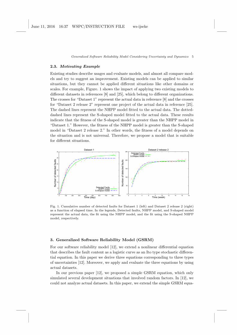
2.3. Motivating Example

Existing studies describe usages and evaluate models, and almost all compare mod-

els and try to suggest an improvement. Existing models can be applied to similar

situations, but they cannot be applied different situations like other domains or

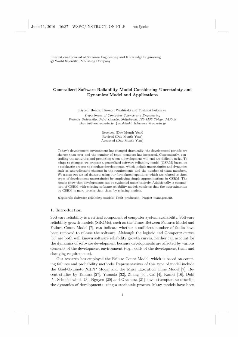
scales. For example, Figure. 1 shows the impact of applying two existing models to

different datasets in references [8] and [25], which belong to different organizations.

The crosses for “Dataset 1” represent the actual data in reference [8] and the crosses

for “Dataset 2 release 2” represent one project of the actual data in reference [25].

The dashed lines represent the NHPP model fitted to the actual data. The dotted-

dashed lines represent the S-shaped model fitted to the actual data. These results

indicate that the fitness of the S-shaped model is greater than the NHPP model in

“Dataset 1.” However, the fitness of the NHPP model is greater than the S-shaped

model in “Dataset 2 release 2.” In other words, the fitness of a model depends on

the situation and is not universal. Therefore, we propose a model that is suitable

for different situations.

0

50

100

150

200

250

0 2 4 6 8 10 12 14 16 18

Num

ber

of dete

cte

d faults

Time (week)

Detected Faults

Dataset 1 Dataset 2 release 2

NHPP modelS-Shaped model

Num

be

r o

f dete

cte

d faults

Time (day)

0

5

10

15

20

25

30

35

0 100 200 300 400 500 600 700 800 900

Detected FaultsNHPP model

S-Shaped model

Fig. 1. Cumulative number of detected faults for Dataset 1 (left) and Dataset 2 release 2 (right)

as a function of elapsed time. In the legends, Detected faults, NHPP model, and S-shaped modelrepresent the actual data, the fit using the NHPP model, and the fit using the S-shaped NHPPmodel, respectively.

3. Generalized Software Reliability Model (GSRM)

For our software reliability model [12], we extend a nonlinear differential equation

that describes the fault content as a logistic curve as an Ito type stochastic differen-

tial equation. In this paper we derive three equations corresponding to three types

of uncertainties [12]. Moreover, we apply and evaluate the three equations by using

actual datasets.

In our previous paper [12], we proposed a simple GSRM equation, which only

simulated several development situations that involved random factors. In [12], we

could not analyze actual datasets. In this paper, we extend the simple GSRM equa-



tion to apply it to actual datasets. The equation is divided into three uncertainty

types: late, constant, and early types. Using clearly defined equations, we apply

GSRMs to actual datasets and obtain the upper and lower limits in each situation

due to random factors, which mean that the GSRM can predict the maximum and

minimum number of faults. Additionally, we evaluate and test our GSRMs and other

models using datasets from different organizations and circumstances. The GSRM

can quantify uncertainties that are influenced by random factors, which is impor-

tant to more accurately model the growth of software reliability and to optimize

development teams or environments.

We start with the logistic differential equation, which is expressed as

dN(t)

dt= N(t)(a+ bN(t)) (5)

N(t) is the number of detected faults by time t, a defines the growth rate, and b is

the carrying capacity. If b = 0, then the solutions are exponential functions. Because

the numerous uncertainties and dynamic changes prevent actual developments from

correctly obeying equation (5), it should be extended into a stochastic differential

equation. We assume that such dynamic elements are time dependent and contain

uncertainties. These elements are expressed using a. The time dependence of a can

be used to describe situations such as an improved development skills and increased

growth rate. The uncertainty of a can describe parameters such as the variability

of development members and the environment. The growth of software is analyzed

with an emphasis on the testing phase by simulating the number of detected faults.

We assume that software development has the following properties:

(1) The total number of faults is constant.

(2) The number of faults that can be found depends on time.

(3) The number of faults that can be found contains uncertainty, which can be

simulated with Gaussian white noise.

The first assumption means that the total number of faults is finite and can

be treated as a boundary condition. This assumption implies that correcting faults

does not create new ones. Indeed, many SRGMs assume that the total number of

faults is constant [18]. Several researchers have proposed SRGMs that can treat

infinite faults [19]. We assume that the debugging process creates new faults. We

suppose that we can use one model for fault creation and fault detection in the

debugging process.

The second assumption means that the ability to detect the faults varies; the

ability depends on time because the number of developers changes in recent de-

velopments, and the number of developers affects the ability to detect the faults.

Researchers have proposed several time dependent models whose situations are

limited such as the error detection per time increases with the progress of software

testing [34]. Hou et al. proposed a SRGM upon considering two learning curves

(the exponential learning curve and the S-shaped learning curve) [13]. These ex-



isting models assume that the number of developers does not change and the time

dependent parameters are a specific model like the exponential learning curve. In

contrast, our model does not depend on a specific model.

The third assumption means that uncertainties in the development process affect

the ability to detect faults. This assumption is due to the fact that actual datasets

have non-constant detection rates or seem to be independent of time. Analyzing

actual faults in datasets, we observed several sudden increases in the number of

detected faults. Then we modeled the uncertainty, which affects the ability to detect

faults as Gaussian white noise that is a simple but commonly used noise. To the

best of our knowledge, other SRGMs do not treat such uncertainties that occur

in the development. By analyzing the uncertainties for each development, we can

understand how a development progresses and predict the progress with a concrete

tolerance.

3.1. Modeling Uncertainties and Dynamics

Considering these properties, equation (5) can be extended to an Ito type stochastic

differential equation with a(t) = α(t) + σ(t)dw(t), which is expressed as

dN(t) = (α(t) + βN(t))N(t)dt+N(t)σ(t)dw(t) (6)

N(t) is the number of detected faults by time t, α(t)+σ(t)dw(t) is the differential of

the number of detected faults per unit time, γ(t) = N(t)σ(t)dw(t) is the uncertainty

term, σ(t) is the dispersion, and β is the nonlinear carrying capacity term. This

equation has two significant terms, α(t) and σ(t)dw(t); α(t) affects the end point of

development and σ(t)dw(t) affects the growth curve through uncertainties. Thus,

our model treats both uncertainties and dynamics. However, uncertainties cannot

be treated directly because they depend on the cause. Our approach treats the

uncertainties through a fault detecting process.

3.2. Uncertainties

In particular, equation (6) indicates that the stochastic term is dependent on N(t),

which means that the uncertainties depend on the number of detected faults. Ac-

cording to equation (6), as the number of detected faults increases, the stochastic

term has a greater effect on the number of detected faults. Such a situation corre-

sponds to software development with late uncertainty.

We compare three different types of dependencies of γ(t) on N(t):

• The late uncertainty type is where γ(t) = N(t)σdw(t).

• The constant uncertainty type is where γ(t) is independent of N(t): γ(t) =

σdw(t).

• The early uncertainty type is where γ(t) depends on the inverse ofN(t): γ(t) =

1/N(t)σdw(t).



As α(t) and the coefficient of dw(t) are varied, models are simulated using equa-

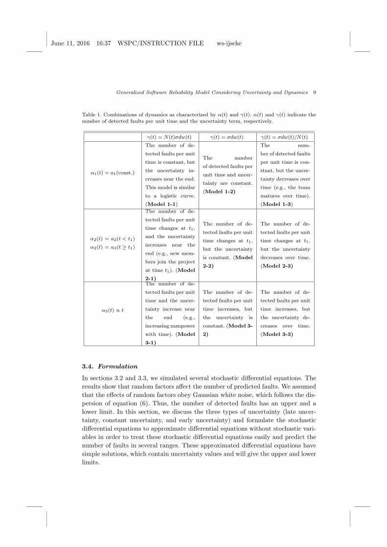
tion (6). Table 1 summarizes the types of α(t), the coefficient of dw(t), and the

corresponding situations. Using GSRM, the type must be chosen for Table 1 to

calculate the parameters using past data. In development, faults are detected and

debugged. The detected faults are counted and used to predict when the project will

end. Projects contain a lot of uncertainty elements, and the predicted development

period is almost never long enough. GSRM can describe the uncertainty of applied

development and calculate the uncertainty of fault detection.

We describe the uncertainty as σ(t)dw(t), which is basically Gaussian white noise

obtained from past data. The uncertainty is difficult to calculate using equation (5),

so we assume some limits and obtain σ(t)dw(t) quantitatively. We start by defining

a(t) in terms of

a(t) = α(t) + σ(t)dw(t) (7)

Equation (5) cannot be solved due to the time dependence of a, as shown in equation

(7). Therefore, we assume that a is time independent with an added term δ, which

is small. This assumption allows equation (5) to be solved. These three uncertainty

types can be rewritten as

dN(t) = (α(t) + βN(t))N(t)dt+N(t)δdw(t) (8)

dN(t) = (α(t) + βN(t))N(t)dt+ δdw(t) (9)

dN(t) = (α(t) + βN(t))N(t)dt+1

N(t)δdw(t) (10)

Each GSRM model is derived from one of these three types of uncertainty.

3.3. Simulations

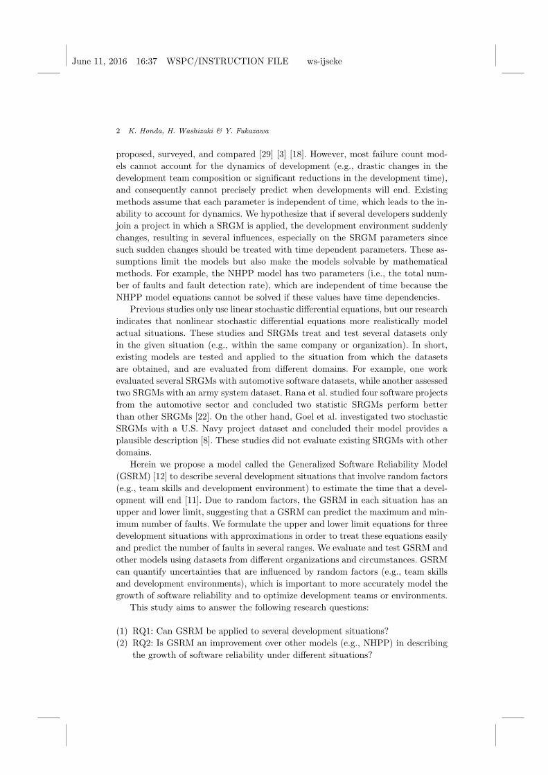
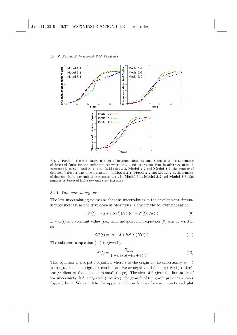
Using these equations for GSRM, we simulated these nine cases. Figure 2 models

and plots these nine cases. For each column in Table 1, the difference between each

model is the parameter α(t). In Model 1-1, Model 2-1 and Model 3-1, which

are based on Model 1-1, a2 = a1, a3 = 2a1 and t1 = tmax/2 in Model 2-1, and

α3(t) = a1t in Model 3-1. α(t)’s are set in the same manner along all columns (i.e.,

α(t) is the same along each row in Table 1). ForModel 1-1,Model 2-1 andModel

3-1, the effect of uncertainty over time, γ(t) = N(t)σdw(t) increases. The situation

in Model 2-1 corresponds to the number of development team members doubling

at time t1. The situation corresponding to Model 3-1 is that the members’ skills

improvement over time, effectively doubling the manpower by the time tmax. For

Model 1-2, Model 2-2, and Model 3-2, the effect of uncertainty γ(t) = σdw(t) is

constant. For Model 1-3, Model 2-3 and Model 3-3, the effect of uncertainty

γ(t) = σdw(t)/N(t) decreases over time.

The purpose of the simulations is to confirm that our approach can assess soft-

ware reliability under dynamic changes and uncertainties in development as well as

adapt the models to produce appropriate results. We used a Monte Carlo method

to examine these models. Figure 2 shows the effects of uncertainties and dynamics.



Table 1. Combinations of dynamics as characterized by α(t) and γ(t). α(t) and γ(t) indicate thenumber of detected faults per unit time and the uncertainty term, respectively.

γ(t) = N(t)σdw(t) γ(t) = σdw(t) γ(t) = σdw(t)/N(t)

α1(t) = a1(const.)

The number of de-

tected faults per unit

time is constant, but

the uncertainty in-

creases near the end.

This model is similar

to a logistic curve.

(Model 1-1)

The number

of detected faults per

unit time and uncer-

tainty are constant.

(Model 1-2)

The num-

ber of detected faults

per unit time is con-

stant, but the uncer-

tainty decreases over

time (e.g., the team

matures over time).

(Model 1-3)

α2(t) = a2(t < t1)

α2(t) = a3(t ≥ t1)

The number of de-


time changes at t1,

and the uncertainty

increases near the

end (e.g., new mem-

bers join the project

at time t1). (Model

2-1)

The number of de-


time changes at t1,

but the uncertainty

is constant. (Model

2-2)

The number of de-


time changes at t1,

but the uncertainty

decreases over time.

(Model 2-3)

α3(t) ∝ t

The number of de-


time and the uncer-

tainty increase near

the end (e.g.,

increasing manpower

with time). (Model

3-1)

The number of de-


time increases, but

the uncertainty is

constant. (Model 3-

2)

The number of de-


time increases, but

the uncertainty de-

creases over time.

(Model 3-3)

3.4. Formulation

In sections 3.2 and 3.3, we simulated several stochastic differential equations. The

results show that random factors affect the number of predicted faults. We assumed

that the effects of random factors obey Gaussian white noise, which follows the dis-

persion of equation (6). Thus, the number of detected faults has an upper and a

lower limit. In this section, we discuss the three types of uncertainty (late uncer-

tainty, constant uncertainty, and early uncertainty) and formulate the stochastic

differential equations to approximate differential equations without stochastic vari-

ables in order to treat these stochastic differential equations easily and predict the

number of faults in several ranges. These approximated differential equations have

simple solutions, which contain uncertainty values and will give the upper and lower

limits.



0

0.2

0.4

0.6

0.8

1

1.2

0 0.2 0.4 0.6 0.8 1Th

e r

ate o

f d

etected

fau

lts Model 1-1

Model 2-1

Model 3-1

Time

0

0.2

0.4

0.6

0.8

1

1.2

0 0.2 0.4 0.6 0.8 1Th

e r

ate o

f d

etected

fau

lts Model 1-2

Model 2-2

Model 3-2

Time

0

0.2

0.4

0.6

0.8

1

1.2

0 0.2 0.4 0.6 0.8 1Th

e r

ate o

f d

etected

fau

lts Model 1-3

Model 2-3

Model 3-3

Time

Fig. 2. Ratio of the cumulative number of detected faults at time t versus the total numberof detected faults for the entire project where the. x-axis represents time in arbitrary units. 1

corresponds to tmax and 0 : 5 to t1. In Model 1-1, Model 1-2 and Model 1-3, the number ofdetected faults per unit time is constant. In Model 2-1, Model 2-2 and Model 2-3, the numberof detected faults per unit time changes at t1. In Model 3-1, Model 3-2 and Model 3-3, thenumber of detected faults per unit time increases.

3.4.1. Late uncertainty type

The late uncertainty type means that the uncertainties in the development circum-

stances increase as the development progresses. Consider the following equation

dN(t) = (α+ βN(t))N(t)dt+N(t)δdw(t) (8)

If δdw(t) is a constant value (i.e., time independent), equation (8) can be written

as

dN(t) = (α+ δ + bN(t))N(t)dt (11)

The solution to equation (11) is given by

N(t) =Nmax

1 + b exp{−(α+ δ)t}(12)

This equation is a logistic equation where δ is the origin of the uncertainty. α + δ

is the gradient. The sign of δ can be positive or negative. If δ is negative (positive),

the gradient of the equation is small (large). The sign of δ gives the limitation of

the uncertainty. If δ is negative (positive), the growth of the graph provides a lower

(upper) limit. We calculate the upper and lower limits of some projects and plot



them in the next section. δ is determined as

δi = − 1

tiln

{1

b

(Nmax

Ni− 1

)}− α (13)

The subscript i indicates the data is for the ith fault detected at ti. i differs from

the approximate value at ti. Finally, we obtain the average and variance of δ. We

can construct the equation of SRGM from the average and variance of δ to simulate

the projects and to predict when they will end by using and its distribution, which

is Gaussian white noise [11]. We assume that the detected faults obey equation (12)

and that the detection rate has a time-independent uncertainty δ. This assumption

yields the following upper and lower limits

N+(t) =Nmax

1 + b exp{−(α+ δ)t}(14)

N−(t) =Nmax

1 + b exp{−(α− δ)t}(15)

N+(t) means the upper limit aboutN(t). If the development proceeds via a favorable

situation, the number of detected faults will obey equation (14). N−(t) denotes the

lower limit about N(t). If the development proceeds via an unfavorable situation,

the number of detected faults will obey equation (15).

3.4.2. Constant uncertainty type

In this section, the constant uncertainty type where the development circumstances

have the uncertainties that are independent of time is discussed. Consider the fol-

lowing equation

dN(t) = (α+ βN(t))N(t)dt+ δdw(t) (9)

If δ → 0, equation (9) is derived as follows

dN(t) = (α+ βN(t))N(t)dt (16)

This equation can be solved as

N(t) =Nmax

1 + b exp(−αt)(17)

This is the base equation for the other types. However if δ << 1 and δ ̸= 0, we

should consider the δ term. The entire term, which is related with δ, is δdw. Because

dw is Gaussian white noise, the value of δ can be calculated from the actual data

and base equation (17). We write the number of the actual detected faults as Ni

and the number of predicted faults as N(t). di, which is the difference between the

actual and predicted data, is defined using these two terms as

di = Ni −N(ti) (18)



δ is expressed as

δ =

√√√√ 1

m

m∑i=1

(di − d̄)2 (19)

δ means the standard deviation. d̄ is the average of di. m represents the total

number of detected faults. Finally, the upper limits and lower limits of the constant

uncertainty type equations are expressed as

N+(t) =Nmax

1 + b exp(−αt)+ δ (20)

N−(t) =Nmax

1 + b exp(−αt)− δ (21)

N+(t) is the upper limits about N(t), while N−(t) means the lower limits about

N(t). These limit equations mean that when the number of detected faults becomes

large, they are not affected by the δ uncertainty term.

3.4.3. Early uncertainty type

In this section, we discuss the early uncertainty type, which means that the uncer-

tainties in the development circumstances decrease in the late stage of the develop-

ment. Consider equation (10), which is given by

dN(t) = (α(t) + βN(t))N(t)dt+ δ1

N(t)dw(t) (10)

If δ → 0, then it can be rewritten as

dN(t) = (α+ βN(t))N(t)dt (22)

This equation can be solved as

N =Nmax

1 + b exp(−αt)(17)

This is the base equation of the other types. However if δ << 1 and δ ̸= 0, then this

should be regarded as the δ term. The whole of the uncertainty term is δdw(t)/N(t).

Because dw(t) is Gaussian white noise, the value of δdw(t)/N(t) can be calculated

from the actual data and base equation (17). The concrete equation is obtained

from equation (17) as

δ{1 + b exp(−αt)}Nmax

(23)

Ni is the number of actual faults and N(t) is the number of predicted faults. di,

which is the difference between the actual data and predicted data, can be expressed

using these two terms as

di = Ni −N(ti) (24)



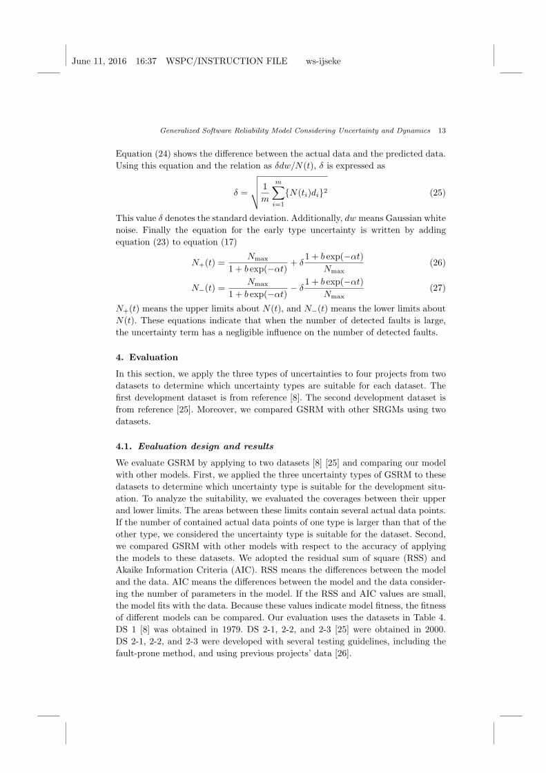
Equation (24) shows the difference between the actual data and the predicted data.

Using this equation and the relation as δdw/N(t), δ is expressed as

δ =

√√√√ 1

m

m∑i=1

{N(ti)di}2 (25)

This value δ denotes the standard deviation. Additionally, dw means Gaussian white

noise. Finally the equation for the early type uncertainty is written by adding

equation (23) to equation (17)

N+(t) =Nmax

1 + b exp(−αt)+ δ

1 + b exp(−αt)

Nmax(26)

N−(t) =Nmax

1 + b exp(−αt)− δ

1 + b exp(−αt)

Nmax(27)

N+(t) means the upper limits about N(t), and N−(t) means the lower limits about

N(t). These equations indicate that when the number of detected faults is large,

the uncertainty term has a negligible influence on the number of detected faults.

4. Evaluation

In this section, we apply the three types of uncertainties to four projects from two

datasets to determine which uncertainty types are suitable for each dataset. The

first development dataset is from reference [8]. The second development dataset is

from reference [25]. Moreover, we compared GSRM with other SRGMs using two

datasets.

4.1. Evaluation design and results

We evaluate GSRM by applying to two datasets [8] [25] and comparing our model

with other models. First, we applied the three uncertainty types of GSRM to these

datasets to determine which uncertainty type is suitable for the development situ-

ation. To analyze the suitability, we evaluated the coverages between their upper

and lower limits. The areas between these limits contain several actual data points.

If the number of contained actual data points of one type is larger than that of the

other type, we considered the uncertainty type is suitable for the dataset. Second,

we compared GSRM with other models with respect to the accuracy of applying

the models to these datasets. We adopted the residual sum of square (RSS) and

Akaike Information Criteria (AIC). RSS means the differences between the model

and the data. AIC means the differences between the model and the data consider-

ing the number of parameters in the model. If the RSS and AIC values are small,

the model fits with the data. Because these values indicate model fitness, the fitness

of different models can be compared. Our evaluation uses the datasets in Table 4.

DS 1 [8] was obtained in 1979. DS 2-1, 2-2, and 2-3 [25] were obtained in 2000.

DS 2-1, 2-2, and 2-3 were developed with several testing guidelines, including the

fault-prone method, and using previous projects’ data [26].



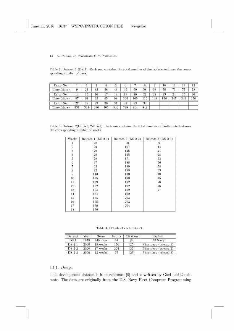
Table 2. Dataset 1 (DS 1). Each row contains the total number of faults detected over the corre-sponding number of days.

Error No. 1 2 3 4 5 6 7 8 9 10 11 12 13

Time (days) 9 21 32 36 43 45 50 58 63 70 71 77 78

Error No. 14 15 16 17 18 19 20 21 22 23 24 25 26

Time (days) 87 91 92 95 98 104 105 116 149 156 247 249 250

Error No. 27 28 29 30 31 32 33 34

Time (days) 337 384 396 405 540 798 814 849

Table 3. Dataset 2(DS 2-1, 2-2, 2-3). Each row contains the total number of faults detected over

the corresponding number of weeks.

Weeks Release 1 (DS 2-1) Release 2 (DS 2-2) Release 3 (DS 2-3)

1 28 90 92 29 107 143 29 126 21

4 29 145 285 29 171 536 37 188 567 63 189 58

8 92 190 639 116 190 7010 125 190 7511 139 192 76

12 152 192 7613 164 192 7714 164 19215 165 203

16 168 20317 170 20418 176

Table 4. Details of each dataset.

Dataset Year Term Faults Citation Explain

DS 1 1979 849 days 34 [8] US Navy

DS 2-1 2000 18 weeks 176 [25] Pharmacy (release 1)



4.1.1. Design

This development dataset is from reference [8] and is written by Goel and Okuk-

moto. The data are originally from the U.S. Navy Fleet Computer Programming



Center and consist of the errors in software development (Table 2). The second

development dataset is from reference [25] and is written by Stringfellow et al. The

data come from three releases of a large medical record system, which consists of 188

software components (Table 3). The data contain the cumulative number of faults

and their detected times for the three different releases of the software program.

We applied GSRM to these datasets and classified the datasets based on the un-

certainty type by comparing the covered actual data points between the upper and

lower limits. To compare with NHPP models (NHPP and S-shaped), we adopted

the time independent model of GSRM because these datasets do not have person

month data. The models were evaluated using RSS and AIC where small values

indicate that the model has a sufficient fit.

Table 4 shows that these datasets contain data from the 1970s and the 2000s,

which were produced by waterfall developments. The 2000s projects were developed

with the fault prone method, which is a modern approach [26]. Therefore, the 2000s

projects were developed via more modern processes than the 1970s project.

4.1.2. Results

We evaluated the adoptions for the three uncertainty types and compared the

GSRMs with NHPP models through the two datasets. For each uncertainty type,

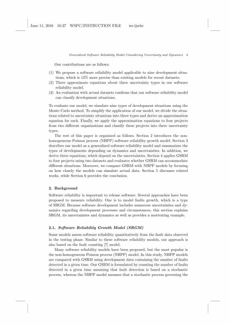
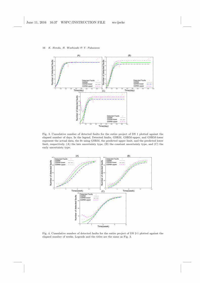
we calculated the upper limit and the lower limit as well as its suitability. Figures 3

– 6 and Table 5 show the results. We compared the GSRMs with the NHPP models

(e.g., the normal NHPP model and S-shaped model) through RSS and AIC. As

mentioned above, small RSS and AIC values indicate a good model fitness. Figure

7 and Table 6 show the results.

Type Selection

We calculated δ and the upper and lower limits. Figures 3 – 6 plot the results where

the x-axis represents time and the y-axis represents the number of detected faults.

Solid, dashed, and dotted-dashed lines represent values calculated with GSRM,

upper limits, and lower limits, respectively. The crosses indicate the actual data in

reference [8] and [25]. These results confirm that almost all of the real data points are

contained within the calculated upper and lower limits. We quantitatively evaluated

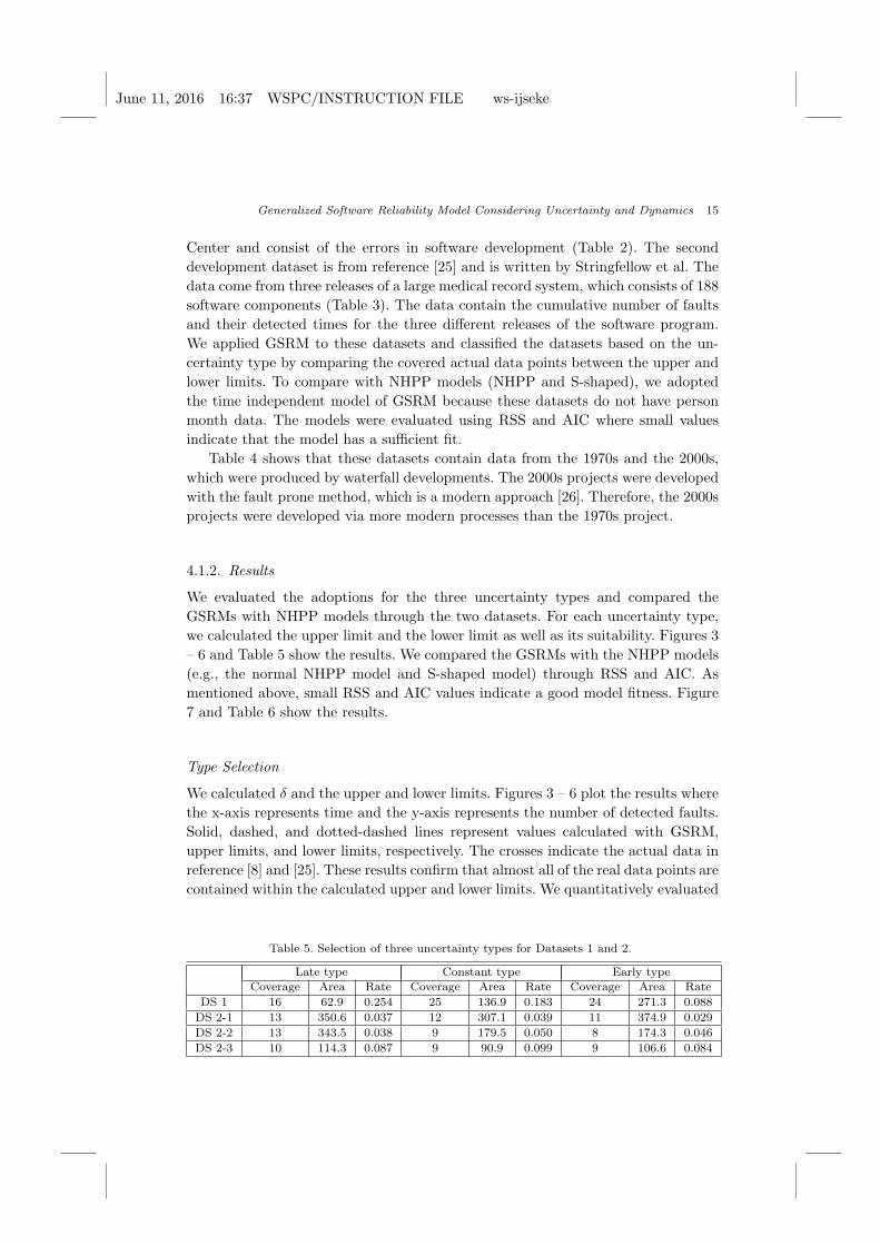
Table 5. Selection of three uncertainty types for Datasets 1 and 2.

Late type Constant type Early typeCoverage Area Rate Coverage Area Rate Coverage Area Rate

DS 1 16 62.9 0.254 25 136.9 0.183 24 271.3 0.088

DS 2-1 13 350.6 0.037 12 307.1 0.039 11 374.9 0.029

DS 2-2 13 343.5 0.038 9 179.5 0.050 8 174.3 0.046

DS 2-3 10 114.3 0.087 9 90.9 0.099 9 106.6 0.084



Nu

mb

er

of

de

tecte

d f

au

lts

Time(day)

(A)

Nu

mb

er

of

de

tecte

d f

au

lts

Time(day)

Time(day)

Nu

mb

er

of

de

tecte

d f

au

lts

GSRM

GSRM-upper

GSRM-lower

Detected Faults

(B)

(C)

0

5

10

15

20

25

30

35

0 100 200 300 400 500 600 700 800 9000

5

10

15

20

25

30

35

0 100 200 300 400 500 600 700 800 900

GSRM

GSRM-upper

GSRM-lower

Detected Faults

0

5

10

15

20

25

30

35

0 100 200 300 400 500 600 700 800 900

GSRM

GSRM-upper

GSRM-lower

Detected Faults

Fig. 3. Cumulative number of detected faults for the entire project of DS 1 plotted against theelapsed number of days. In the legend, Detected faults, GSRM, GSRM-upper, and GSRM-lowerrepresent the actual data, the fit using GSRM, the predicted upper limit, and the predicted lower

limit, respectively. (A) the late uncertainty type, (B) the constant uncertainty type, and (C) theearly uncertainty type.

0

50

100

150

200

0 5 10 15 20

GSRM

GSRM-upper

GSRM-lower

Detected Faults

GSRM

GSRM-upper

GSRM-lower

Detected Faults

0

50

100

150

200

0 5 10 15 20

Num

be

r of dete

cte

d faults

Time(week)

(A)

Num

be

r of dete

cte

d faults

Time(week)

Num

be

r of dete

cte

d faults

0

50

100

150

200

0 5 10 15 20

GSRM

GSRM-upper

GSRM-lower

Detected Faults

Time(week)

(B)

(C)

Fig. 4. Cumulative number of detected faults for the entire project of DS 2-1 plotted against the

elapsed number of weeks. Legends and the titles are the same as Fig. 3.



0

50

100

150

200

250

0 2 4 6 8 10 12 14 16 18

0

50

100

150

200

250

0 2 4 6 8 10 12 14 16 18

GSRM

GSRM-upper

GSRM-lower

Detected Faults

0

50

100

150

200

250

0 2 4 6 8 10 12 14 16 18

GSRM

GSRM-upper

GSRM-lower

Detected Faults

GSRM

GSRM-upper

GSRM-lower

Detected Faults

Num

be

r of dete

cte

d faults

Time(week)

(A)

Time(week)

Num

be

r of dete

cte

d faults

Time(week)

(B)

Num

be

r of dete

cte

d faults

(C)

Fig. 5. Cumulative number of detected faults for the entire project of DS 2-2 plotted against the

elapsed number of weeks. Legends and the titles are the same as Fig. 3.

0

20

40

60

80

100

0 2 4 6 8 10 12 140

20

40

60

80

100

0 2 4 6 8 10 12 14

GSRM

GSRM-upper

GSRM-lower

Detected FaultsGSRM

GSRM-upper

GSRM-lower

Detected Faults

0

20

40

60

80

100

0 2 4 6 8 10 12 14

GSRM

GSRM-upper

GSRM-lower

Detected Faults

Num

be

r of dete

cte

d faults

Time(week)

(A)

Num

be

r of dete

cte

d faults

Time(week)

(B)

Num

be

r of dete

cte

d faults

Time(week)

(C)

Fig. 6. Cumulative number of detected faults for the entire project of DS 2-3 plotted against theelapsed number of weeks. Legends and titles are the same as Fig. 3.



which type is suitable for each datasets by calculating the Coverage, Area, and Rate

for each dataset. Coverage means the number of actual data points between the

upper and lower limits. Area, which denotes the area surrounded by the upper and

lower models, is calculated by integrating the upper and lower models. Rate, which

indicates the coverage rate of the type, represents the Coverage divided by Area.

Coverage is the most important value since a model with a large Coverage can cover

a lot of actual data points. If one type has a larger Coverage than the other types,

it is more suitable for the dataset. However, if the types have equal Coverage, then

the type with the largest Rate is most suitable for the dataset.

Table 5 shows the results. The constant type of uncertainty is suitable for dataset

1 because it has the largest coverage (Figure. 3 and Table 6). This is reasonable

since the interval of detecting faults is random as the development proceeds in

dataset 1, indicating that uncertainty events randomly occur. The results of release

1, 2, and 3 indicate that the late type is suitable for dataset 2 because it has the

largest coverage (Figures. 4 -窶 6). This is consistent with Tables 3 and 6 where

more faults are detected at the end of development for dataset 2, indicating that

the development has issues up until each release.

In these datasets, we could not verify the results by interviewing the development

teams that produced these datasets due to the age of the datasets. Therefore, we

requested that a Japanese IT company, which employs about 5000 people, use

GSRMs and evaluate the results, including the uncertainties, from 2013 to 2015.

We collected the fault datasets from the two projects in the company. Additionally,

the two managers of the two development teams evaluated the results. Then we

asked the two managers about the GSRM results and whether they agreed with the

uncertainty type according to the GSRMs. They responded that the uncertainty

type indicated by the results is consistent with their thoughts.

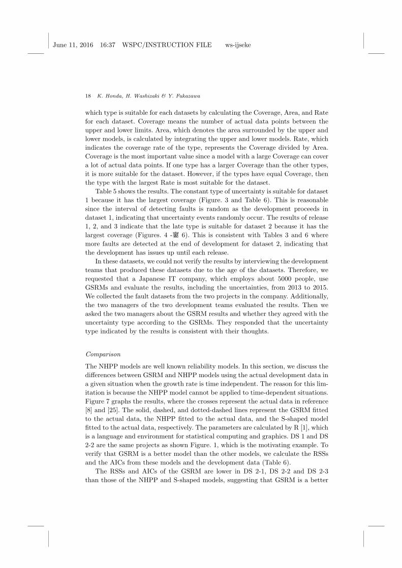
Comparison

The NHPP models are well known reliability models. In this section, we discuss the

differences between GSRM and NHPP models using the actual development data in

a given situation when the growth rate is time independent. The reason for this lim-

itation is because the NHPP model cannot be applied to time-dependent situations.

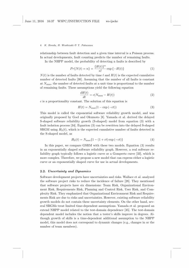
Figure 7 graphs the results, where the crosses represent the actual data in reference

[8] and [25]. The solid, dashed, and dotted-dashed lines represent the GSRM fitted

to the actual data, the NHPP fitted to the actual data, and the S-shaped model

fitted to the actual data, respectively. The parameters are calculated by R [1], which

is a language and environment for statistical computing and graphics. DS 1 and DS

2-2 are the same projects as shown Figure. 1, which is the motivating example. To

verify that GSRM is a better model than the other models, we calculate the RSSs

and the AICs from these models and the development data (Table 6).

The RSSs and AICs of the GSRM are lower in DS 2-1, DS 2-2 and DS 2-3

than those of the NHPP and S-shaped models, suggesting that GSRM is a better



0

50

100

150

200

250

0 2 4 6 8 10 12 14 16 180

10

20

30

40

50

60

70

80

90

0 2 4 6 8 10 12 14

Num

ber

of dete

cte

d faults

Time (day)

DS 1

Detected FaultsGSRM


0

20

40

60

80

100

120

140

160

180

200

0 5 10 15 20

DS 2-1

Time (week)

Detected FaultsGSRM


Num

ber

of dete

cte

d faults

Num

ber

of dete

cte

d faults

Time (week)

DS 2-2

Detected FaultsGSRM


Detected FaultsGSRM


Num

ber

of dete

cte

d faults

Time (week)

DS 2-3

0

5

10

15

20

25

30

35

0 100 200 300 400 500 600 700 800 900

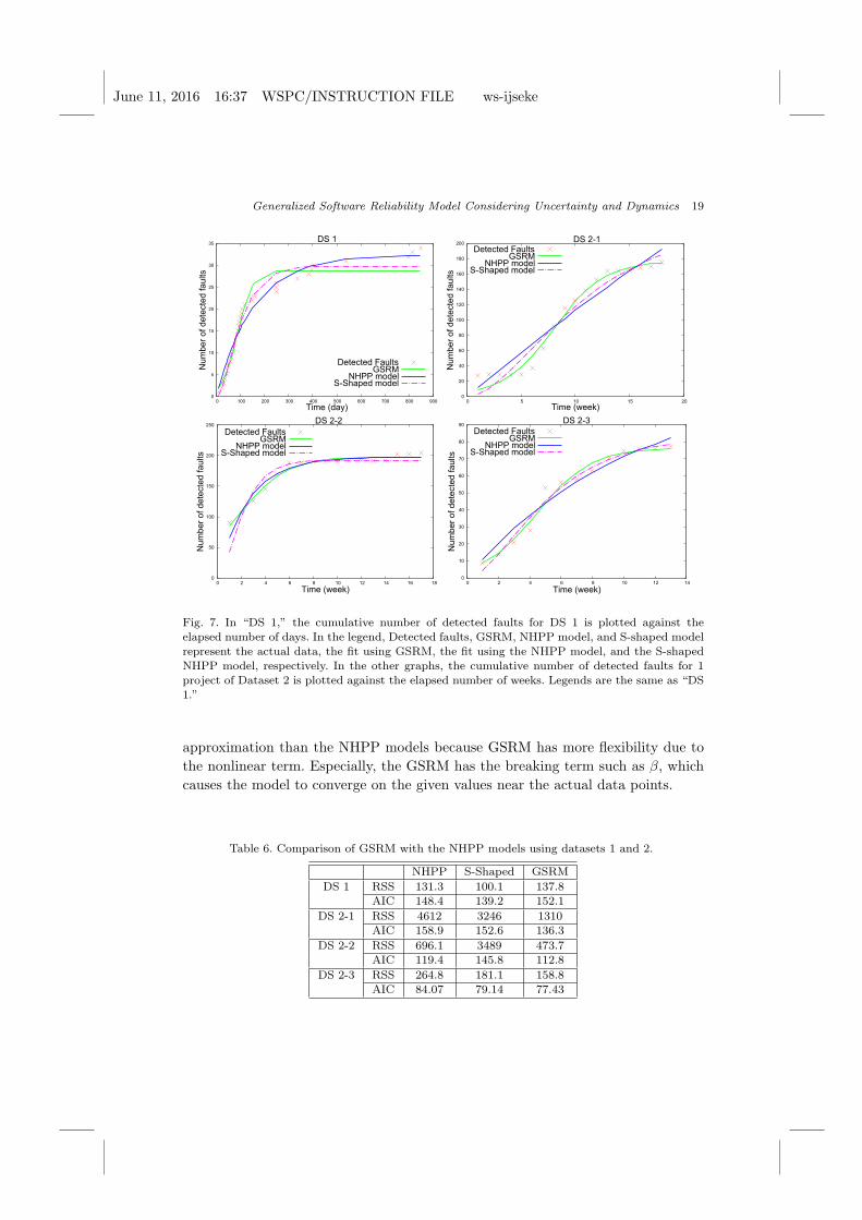
Fig. 7. In “DS 1,” the cumulative number of detected faults for DS 1 is plotted against theelapsed number of days. In the legend, Detected faults, GSRM, NHPP model, and S-shaped model

represent the actual data, the fit using GSRM, the fit using the NHPP model, and the S-shapedNHPP model, respectively. In the other graphs, the cumulative number of detected faults for 1project of Dataset 2 is plotted against the elapsed number of weeks. Legends are the same as “DS1.”

approximation than the NHPP models because GSRM has more flexibility due to

the nonlinear term. Especially, the GSRM has the breaking term such as β, which

causes the model to converge on the given values near the actual data points.

Table 6. Comparison of GSRM with the NHPP models using datasets 1 and 2.

NHPP S-Shaped GSRM

DS 1 RSS 131.3 100.1 137.8AIC 148.4 139.2 152.1

DS 2-1 RSS 4612 3246 1310AIC 158.9 152.6 136.3

DS 2-2 RSS 696.1 3489 473.7AIC 119.4 145.8 112.8

DS 2-3 RSS 264.8 181.1 158.8

AIC 84.07 79.14 77.43



4.2. Discussion

We compared GSRM with other NHPP models using two datasets in order to assess

whether GSRM can describe the data precisely. Additionally, we applied the three

uncertainty types to the datasets to verify whether GSRM can adapt to different

situations.

4.2.1. Wide applicability (RQ1)

In our simulations, we applied the reliability growth models to nine types of devel-

opment situations, which are characterized by two uncertainty elements related to

the detection of faults.

We successfully simulated the three types of dynamics of the development sit-

uation: the number of detected faults per unit time is constant (e.g., the number

of members is constant), the number of detected faults per unit time changes at

the given time (e.g., new members join the project a given time) and the num-

ber of detected faults per unit time increases (e.g., new members join the project

gradually). Especially, for the type where the number of detected faults per unit

time increases, the number of detected faults is smaller than the other types in

the late development, but it is greater than the other types in early development.

This means that if new members join the project gradually, the number of detected

faults will be smaller than other types at the late of the development. If managers

decided to increase the members at the early development, ideally they would add

new members all at once and not gradually.

Existing models can describe only one of these situations with additional limita-

tions, but GSRM can describe several of these situations primarily because existing

models cannot handle time-dependent growth rates without limitations, whereas

GSRM can handle time-dependent rates as long as the appropriate uncertainty sit-

uation is inputted. Additionally, GSRM has a scheme for development uncertainties

and can construct a model involving uncertainties.

GSRM has a good fit for almost all datasets. The S-shape model has a good fit

for several datasets, but a worse fit for other datasets (e.g., dataset 2, release 2),

indicating that the appropriateness of the model depends on the situation. GSRM

shows that dataset 2, release 2 is the late uncertainty type, while the other releases

have similar coverages for the different uncertainty types. The results suggest that

dataset 2, release 2 may be complicated since many faults are detected in the first

week. Regardless, these results indicate that GSRM can treat several situations.

The old dataset (e.g., dataset 1) is a constant type of GSRM, while the new

datasets (e.g., dataset 2) are late types of GSRM. This means that the old devel-

opment has uncertainty events throughout development, while the new develop-

ment has uncertainty events at the later stage of development. Nowadays, many

researchers and developers recommend that faults or bugs be removed at the ear-

lier stages of development. We assume that the new development would be well

controlled since modern developers may have more skills and knowledge than tradi-



tional developers. On the other hand, we assume that the old development would be

always exposed to uncertainty events since developers may not have sophisticated

skills and specific knowledge.

4.2.2. Comparison with other models (RQ2)

Given a situation where the growth rate is time independent, we used two actual

datasets to compare to GSRM with the NHPP models. The results show a high-

precision convergence of the numbers of faults and appropriate development terms

with GSRM. The precision of convergence is at least 12% higher for GSRM than

for the NHPP models, confirming that GSRM can describe software growth more

realistically than previously proposed models based on the NHPP models. Thus,

using GSRMmay help developers devise a more accurate plan for releasing software.

4.3. Limitations

We derive three uncertainty types by considering development situations artificially.

However, the three types are intuitive.

To verify the probability of the types (late type, constant type, and early type),

we interviewed several developers about whether these three types are suitable for

actual developments. Almost all developers responded affirmatively and answered

that their experiments seem to correspond to these types. Although one developer

answered that there are other uncertainty types, the framework that the product

employed in his experiment was forced to suddenly change to another framework

mid-development. Although we propose three types of uncertainties in development

as an initial study, it is true that there are other types of uncertainties.

4.3.1. Threats to Internal Validity

We treated the growth of the number of faults as a time dependent function. The

growth of the number of faults may be related to other factors (e.g., test efforts).

In this research, we could not collect and evaluate the test efforts and other data.

The test efforts should influence the number of the detected faults because if the

test efforts are not constant, the number of detected faults changes.

We chose three types of uncertainty: late, constant, and early. It is not necessary

to divide the uncertainty types by time categories. Although the responses vary by

individual, we asked several developers whether their assessment agreed with the

uncertainty type of the GSRM. Overall, the developers’ thoughts were consistent

with the uncertainty types.

In comparing the models, we used two datasets, both of which were obtained by

one organization or company. It is possible that the data contains mistakes or other

false elements. Several studies have focused on the accuracy of the faults datasets.

An early paper on bug reports in open software indicates that the bug reports

often contain information that does not describe bugs [10]. However, the datasets



we used were collected from industries. In general, industries try to collect exact

bug reports because they do not want to release software with bugs. If bugs remain

in software released to other companies, the bugs may have a detrimental effect.

Thus, products developed by industries tend to contain few faults. In [25], products

related to dataset 2 have few faults in each release. Hence, the number of mistakes

remaining in the dataset does not greatly impact our research results.

Additionally, the data were too old to compare with recent developments. How-

ever, recent studies have also employed these datasets, which should protect the

validity of the results of this study.

4.3.2. Threats to External Validity

We only tested GSRM with two datasets, which is insufficient to make generaliza-

tions about GSRM. Moreover, the datasets are old and the scales of their systems

are smaller than recent systems. Although a lot of factors (e.g., development styles,

development scales, organizations, ages, etc.) should greatly affect the growth of

the number of faults, we could not evaluate such factors. We evaluated two datasets

belonging to a different organization published in different timeframes.

In the future, we plan to use datasets related to large-scale systems. Moreover,

we plan to use datasets with different development styles or development scales.

Additionally, we only compared GSRM with NHPP models. However, other models

exist. Although these models have similar origins as the NHPPmodel, GSRM should

be compared to other models besides NHPP models.

4.3.3. Threats to Construct Validity

We supposed that the uncertainty types of developments can be categorized as late

type, constant type, and early type, and can be evaluated by applying GSRM to

actual datasets. The types of uncertainties were artificial and may not be applicable

to actual datasets because it is possible that the datasets belong to other uncertainty

types.

Additionally, it is unclear whether we evaluated the correct uncertainty values

by applying GSRMs to the datasets quantitatively since our definitions of the uncer-

tainty values were built from only the viewpoints of the number of faults and time

series. However, several developers who understood the results of GSRM concurred

with the types determined by GSRM.

5. Related works

5.1. Software Reliability Growth Models

Many kinds of software reliability growth models exist. Several researchers proposed

time-dependent models whose situations are limited such as the error detection per

time increase with the progress of software testing [34]. Yamada et al. proposed an



extend NHPP model, which is related with test-domain dependence [35]. The test-

domain dependent model includes the idea that the tester’s skills should improve by

degrees (e.g., the growth of skills is time dependent). Hou et al. proposed a SRGM

considering two learning curves, which are the exponential learning curve and the

S-shaped learning curve [13]. These models assume that the number of developers

does not change and the time dependent parameters are model specific like the

exponential learning curve. Our model does not depend on such specific models

and situations.

Although software reliability models have not been used on waterfall develop-

ment, Fujii et al. developed a quantitative software reliability assessment method in

incremental development processes, which is an agile software development, based

on the familiar non-homogeneous Poisson processes [6]. They used not only the

number of faults but also software metrics, which are the number of software mod-

ules, the number of design reviews, the number of test cases performed, the size of

software, and the development effort. They showed a software reliability prediction

through a case study. They developed a SRGM for the incremental development

processes and adopted other metrics to their SRGM, but they did not directly treat

the number of developers. Our model can directly treat the number of developers,

which should be suitable to actual and recent development styles.

Kuo et al. proposed a framework for modeling the software reliability model

using various testing efforts and fault detection rates [17]. The testing efforts mean

the resource expenditures spent on software testing (e.g., test cases, human resource,

CPU time) applied into SRGMs in [31]. Kuo et al. applied their framework to several

NHPP models by employing three types of testing effort functions (constant testing

effort consumption, Weibull-type testing effort function, and Logistic testing effort

functions) and two types of fault detection rates (constant proportionality and time-

variable fault detection rates).

Additionally, Ahmad et al. proposed an S-shaped NHPP model containing

testing-effort [2]. Ahmad et al. assumed that the testing effort expenditures are

described by the Log-logistic function and integrated the Log-logistic function into

an S-shaped NHPP model. Their model requires the test effort expenditures such

as the test cases and human resource, but our model only needs the number of

developers.

Huang et al. proposed five SRGMs with multiple changing points, which could

be treated as the timing of introducing new tools or techniques [14]. They prepared

datasets with and without multiple changing points, and evaluated their SRGMs

with the changing points and the estimated changing points. Their idea about

multiple changing points in development is similar to our assumption about dynamic

changes in development. However, they only target the timing of the changes of

development, whereas our model targets the timing and the concrete values such

as the increased numbers of developers. Since our model can treat concrete values

such as the numbers developers, we are able to simulate the development in section



3.3.

Singh et al. proposed a SRGM using a feed forward neural network approach,

which is a machine learning method [24]. Their approach uses part of the data

(60% to 80% from the beginning) for several datasets to train each neural network

model. We supposed that if several development changes occur after learning data

their model would not be able to treat such situations since it was constructed

with the learning data using a machine learning technique. Our model can treat a

situation such as changes in developers, which we simulate in section 3.3.

5.2. Uncertainties

Several researchers tried to treat the uncertainties in requirements and operations.

Wallace et al. studied the risk [28] and analyzed the software project risks to reduce

the incidence of failure [28]. They mentioned that software projects have six dimen-

sions: Team Risk, Organizational Environment Risk, Requirements Risk, Planning

and Control Risk, User Risk, and Complexity Risk. They emphasized that Organiza-

tional Environment Risk and Requirements Risk are due to risks and uncertainties.

Our studies focus on the uncertainties and try to evaluate the uncertainties in a

quantitative manner. In contrast, Wallace et al. did not focus on the uncertainties

and did not evaluate the uncertainties in a quantitative way.

Goseva-Popstojanova and Kamavaram studied the uncertainties in requirements

and operations by component-based software engineering [15] [9]. In [15], they an-

alyzed the uncertainties of operational profiles and component reliability by calcu-

lating the conditional entropy of each component. In [9], they analyzed the uncer-

tainties of the operational profiles and the component reliability by Monte Carlo

simulations. These analytic methods focus on the requirements and operations.

However, our methods focus on the uncertainties in development phases, including

requirements and operations. In the future, we plan to analyze the effects of the un-

certainties in requirements and operations since we suppose that the uncertainties

in the requirement phases affect the development process.

6. Conclusion

Using GSRM, we successfully simulated developments containing uncertainties and

dynamic elements. We obtained the time-dependent logistic curve and growth curve,

which is not possible using other models, as well as simulated and analyzed nine

types of developments with GSRM. Additionally, we formulated equations for three

types of uncertainty that are related to actual development situations. We also

defined uncertainty values from actual data containing information on faults during

development and applied GSRM to datasets to calculate the fitness of the models.

These results demonstrate that GSRM can calculate uncertainties using past data

and predict how long a project will take.

In the future, we plan to evaluate teams or team members using quantitative

methods while considering uncertainties to optimize teams for a particular project



using GSRM.

References

[1] The r project for statistical computing. http://www.r-project.org/.[2] N. Ahmad, M. G. Khan, and L. S. Rafi. Analysis of an inflection s-shaped software

reliability model considering log-logistic testing-effort and imperfect debugging. In-ternational Journal of Computer Science and Network Security, 11(1):161–171, 2011.

[3] M. Anjum, M. A. Haque, and N. Ahmad. Analysis and ranking of software relia-bility models based on weighted criteria value. International Journal of InformationTechnology and Computer Science (IJITCS), 5(2):1, 2013.

[4] X. Cai and M. Lyu. Software reliability modeling with test coverage: Experimentationand measurement with a fault-tolerant software project. In Software Reliability, 2007.ISSRE ’07. The 18th IEEE International Symposium on, pages 17–26, Nov 2007.

[5] T. Dohi, K. Yasui, and S. Osaki. Software reliability assessment models basedon cumulative bernoulli trial processes. Mathematical and computer modelling,38(11):1177–1184, 2003.

[6] T. Fujii, T. Dohi, and T. Fujiwara. Towards quantitative software reliability assess-ment in incremental development processes. In Proceedings of the 33rd InternationalConference on Software Engineering, ICSE ’11, pages 41–50, New York, NY, USA,2011. ACM.

[7] A. Goel. Software reliability models: Assumptions, limitations, and applicability. Soft-ware Engineering, IEEE Transactions on, SE-11(12):1411–1423, Dec 1985.

[8] A. L. Goel and K. Okumoto. Time-dependent error-detection rate model for softwarereliability and other performance measures. IEEE transactions on Reliability, 3:206–211, 1979.

[9] K. Goseva-Popstojanova and S. Kamavaram. Assessing uncertainty in reliability ofcomponent-based software systems. In Software Reliability Engineering, 2003. ISSRE2003. 14th International Symposium on, pages 307–320, Nov 2003.

[10] K. Herzig, S. Just, and A. Zeller. It's not a bug, it's a feature: Howmisclassification impacts bug prediction. In Proceedings of the 2013 InternationalConference on Software Engineering, ICSE ’13, pages 392–401, Piscataway, NJ, USA,2013. IEEE Press.

[11] K. Honda, H. Nakai, H. Washizaki, Y. Fukazawa, K. Asoh, K. Takahashi, K. Ogawa,M. Mori, T. Hino, Y. HAYAKAWA, et al. Predicting time range of development basedon generalized software reliability model. In 21st Asia-Pacific Software EngineeringConference (APSEC 2014), 2014.

[12] K. Honda, H. Washizaki, and Y. Fukazawa. A generalized software reliability modelconsidering uncertainty and dynamics in development. In J. Heidrich, M. Oivo,A. Jedlitschka, and M. Baldassarre, editors, Product-Focused Software Process Im-provement, volume 7983 of Lecture Notes in Computer Science, pages 342–346.Springer Berlin Heidelberg, 2013.

[13] R.-H. Hou, S.-Y. Kuo, and Y.-P. Chang. Applying various learning curves to hyper-geometric distribution software reliability growth model. In Software Reliability Engi-neering, 1994. Proceedings., 5th International Symposium on, pages 8–17, Nov 1994.

[14] C.-Y. Huang and M. R. Lyu. Estimation and analysis of some generalized mul-tiple change-point software reliability models. Reliability, IEEE Transactions on,60(2):498–514, 2011.

[15] S. Kamavaram and K. Goseva-Popstojanova. Entropy as a measure of uncertaintyin software reliability. In 13th Int ’l Symp. Software Reliability Engineering, pages



209–210, 2002.[16] Y. Kamei, A. Monden, and K.-i. Matsumoto. Empirical evaluation of svm-based

software reliability model. In Proc. Fifth ACM/IEEE Int’l Symp. Empirical SoftwareEng, volume 2, pages 39–41, 2006.

[17] S.-Y. Kuo, C.-Y. Huang, and M. R. Lyu. Framework for modeling software reliability,using various testing-efforts and fault-detection rates. Reliability, IEEE Transactionson, 50(3):310–320, 2001.

[18] R. Lai and M. Garg. A detailed study of nhpp software reliability models. Journal ofSoftware, 7(6):1296–1306, 2012.

[19] J. D. Musa and K. Okumoto. A logarithmic poisson execution time model for soft-ware reliability measurement. In Proceedings of the 7th International Conference onSoftware Engineering, ICSE ’84, pages 230–238, Piscataway, NJ, USA, 1984. IEEEPress.

[20] E. Nguyen, C. Rexach, D. Thorpe, and A. Walther. The importance of data qualityin software reliability modeling. In Software Reliability Engineering (ISSRE), 2010IEEE 21st International Symposium on, pages 220–228, Nov 2010.

[21] H. Okamura, Y. Etani, and T. Dohi. A multi-factor software reliability model basedon logistic regression. In Software Reliability Engineering (ISSRE), 2010 IEEE 21stInternational Symposium on, pages 31–40, Nov 2010.

[22] R. Rana, M. Staron, C. Berger, J. Hansson, M. Nilsson, and F. Torner. Evaluat-ing long-term predictive power of standard reliability growth models on automotivesystems. In Software Reliability Engineering (ISSRE), 2013 IEEE 24th InternationalSymposium on, pages 228–237, Nov 2013.

[23] N. Schneidewind and M. Hinchey. A complexity reliability model. In Software Relia-bility Engineering, 2009. ISSRE ’09. 20th International Symposium on, pages 1–10,Nov 2009.

[24] Y. Singh and P. Kumar. Prediction of software reliability using feed forward neu-ral networks. In Computational Intelligence and Software Engineering (CiSE), 2010International Conference on, pages 1–5. IEEE, 2010.

[25] C. Stringfellow and A. Andrews. An empirical method for selecting software reliabilitygrowth models. Empirical Software Engineering, 7(4):319–343, 2002.

[26] C. V. Stringfellow. An integrated method for improving testing effectiveness andefficiency. 2007.

[27] Y. Tamura and S. Yamada. A flexible stochastic differential equation model indistributed development environment. European Journal of Operational Research,168(1):143–152, 2006.

[28] L. Wallace, M. Keil, and A. Rai. Understanding software project risk: a cluster anal-ysis. Information & Management, 42(1):115–125, 2004.

[29] K. Worwa. A discrete-time software reliability-growth model and its application forpredicting the number of errors encountered during program testing. Control andCybernetics, 34(2):589, 2005.

[30] S. Yamada. Recent developments in software reliability modeling and its applications.In Stochastic Reliability and Maintenance Modeling, pages 251–284. Springer, 2013.

[31] S. Yamada, J. Hishitani, and S. Osaki. Software-reliability growth with a weibull test-effort: a model and application. IEEE Transactions on Reliability, 42(1):100–106, Mar1993.

[32] S. Yamada, M. Kimura, H. Tanaka, and S. Osaki. Software reliability measurementand assessment with stochastic differential equations. IEICE transactions on funda-mentals of electronics, communications and computer sciences, 77(1):109–116, 1994.

[33] S. Yamada, M. Ohba, and S. Osaki. S-shaped reliability growth modeling for software



error detection. Reliability, IEEE Transactions on, R-32(5):475–484, Dec 1983.[34] S. Yamada, M. Ohba, and S. Osaki. s-shaped software reliability growth models and

their applications. Reliability, IEEE Transactions on, R-33(4):289–292, 1984.[35] S. Yamada, H. Ohtera, and M. Ohba. Testing-domain dependent software reliability

models. Computers and Mathematics with Applications, 24(12):79 – 86, 1992.[36] N. Zhang, G. Cui, and H. Liu. A stochastic software reliability growth model with

learning and change-point. In World Automation Congress (WAC), 2012, pages 399–403, June 2012.

generalized software reliability model considering ...software reliability growth model (srgm) some...

Documents