generalizedﬁniteelementmethods forquadraticeigenvalueproblems · mis the mass matrix, is the...

Wegelerstraße • Bonn • Germanyphone + - • fax + -

www.ins.uni-bonn.de

Axel Målqvist and Daniel Peterseim

Generalized finite element methodsfor quadratic eigenvalue problems

INS Preprint No. 1522

Oct 2015

GENERALIZED FINITE ELEMENT METHODS FORQUADRATIC EIGENVALUE PROBLEMS

AXEL MALQVIST AND DANIEL PETERSEIM

Abstract. We consider a large-scale quadratic eigenvalue prob-lem (QEP), formulated using P1 finite elements on a fine scale ref-erence mesh. This model describes damped vibrations in a struc-tural mechanical system. In particular we focus on problems withrapid material data variation, e.g., composite materials. We con-struct a low dimensional generalized finite element (GFE) spacebased on the localized orthogonal decomposition (LOD) technique.The construction involves the (parallel) solution of independent lo-calized linear Poisson-type problems. The GFE space is then usedto compress the large-scale algebraic QEP to a much smaller onewith a similar modeling accuracy. The small scale QEP can thenbe solved by standard techniques at a significantly reduced com-putational cost. We prove convergence with rate for the proposedmethod and numerical experiments confirm our theoretical find-ings.

1. Introduction

Quadratic eigenvalue problems appear in various engineering disci-plines. Often they are the result of finite element modeling ratherthan established partial differential equations. A classical example isa damped vibrating structure. For a spatially discretized structure wehave,

(1.1) Kz + λDz + λ2Mz = 0,

Date: October 19, 2015.2000 Mathematics Subject Classification. 65N30, 65N25, 65N15.Key words and phrases. quadratic eigenvalue problem, finite element, localized

orthogonal decomposition.A. Malqvist is supported by the Swedish Research Council and the Swedish

foundation of strategic research.D. Peterseim is supported by the Hausdorff Center for Mathematics Bonn and

by Deutsche Forschungsgemeinschaft in the Priority Program 1748 ”Reliable sim-ulation techniques in solid mechanics. Development of non-standard discretiza-tion methods, mechanical and mathematical analysis” under the project ”Adap-tive isogeometric modeling of propagating strong discontinuities in heterogeneousmaterials”.

1

2 AXEL MALQVIST AND DANIEL PETERSEIM

where K is the finite element stiffness matrix, D is the damping matrix,M is the mass matrix, λ is the eigenvalue, and z is the correspondingeigenvector. Assuming all matrices to be real there are 2n finite eigen-values (n being the dimension of the matrices) that are real or complexconjugate. Furthermore, if z is a right eigenvector of λ then z is a righteigenvector of z. If D is also symmetric the left and right eigenvectorsare equal. See [25] for a more detailed discussion on how the spec-trum and eigenspaces depend on properties of the matrices, and for anextensive overview of applications see [25, 17, 4, 15].

We will use a specific finite element realization of the more generalformulation presented in Equation (1.1) as a starting point for thiswork. We seek an eigenvalue λ ∈ C and eigenfunction u ∈ V FE

h , whereV FE

h is a finite element space, such that,

(κ∇u,∇v) + λd(u, v) + λ2(u, v) = 0, ∀v ∈ V FEh ,

where the three bilinear forms in the left hand side corresponds to thethree matrices K, D, and M in Equation (1.1). In particular we areinterested in problems where the coefficient κ varies rapidly in spacemodeling, e.g., rapid material data variation. It is well known that inorder to capture the correct behavior of the solution, the finite elementspace V FE

h has to be large enough to resolve the data variations [2].In this paper, we will not question the properness of this model. Weassume that the parameter h was carefully chosen in an earlier modelingor discretization step.

There are various models for the damping. The simplest one is pro-portional damping where D = α0K + α1M with α0, α1 ∈ R using thematrix notation. In this case the eigenmodes actually coincide with theeigenmodes of the linear generalized eigenvalue problem Kx = λMxbut with different eigenvalues. If a structure is made up of differentcomponents (or materials) each of the parts may be modeled usingproportional damping with different constants. The full structure willthen have spatially varying damping parameters α0, α1 and the damp-ing will therefore not be proportional. In this work we will treat ageneral abstract damping bilinear form d but in the numerical experi-ments we will focus on mass and stiffness type damping with spatiallyvarying parameters.

Numerical algorithms for solving quadratic eigenvalue problems areoften based on linearization [17, 15, 4]. This technique results in alinear, possibly non-symmetric, generalized eigenvalue problem. In thisapproach, the size of the system gets doubled which, in the presence ofmultiscale features (since the initial finite element space has to be verylarge) is a drawback. Another drawback might be that the underlying

GFEM FOR QUADRATIC EIGENVALUE PROBLEMS 3

structure of the quadratic eigenvalue problem can be lost. There arealso numerical schemes that can be applied directly to the quadraticeigenvalue problem without linearization, e.g., [25]. In this paper, wewill work with the linearized system.

While the literature in this context of numerical linear algebra isrich, results on error analysis and convergence of finite element ap-proximations to quadratic eigenvalue problems are rather limited [3].To our best knowledge, the literature on GFEMs or multiscale meth-ods for eigenvalue problems is limited to [20] which treats the linearcase. Since linearization is a natural approach also when analyzingfinite element approximations to quadratic eigenvalue problems, theliterature on non-symmetric generalized eigenvalue problems is veryrelevant. Standard references include [16, 1, 5] and for non-compactoperators [9, 10]. These works gives a mathematical foundation for theconvergence analysis presented in this paper.

This paper neither aims to improve existing linear algebra techniquesfor solving quadratic eigenvalue problems nor to invent new ones. Theaim is to reduce the size of the system before applying any of thestandard solvers and, thereby, to speed-up the overall computation sig-nificantly. This will be achieved by constructing a computable lowdimensional subspace of V FE

h , based on the framework of localized or-thogonal decomposition (LOD) [19, 20]. The space captures the mainfeatures of the eigenspaces and, in particular, the effect of the rapidoscillations induced by the rough diffusion coefficient κ. Given this lowdimensional space we can solve the quadratic eigenvalue problem at agreatly reduced computational cost while the accuracy is largely pre-served. Under weak assumptions on the damping, the error analysisshows that the GFEM approximation is very accurate (in the senseof super convergence) when compared to the reference finite elementsolution, independent of the variations in the multiscale data. Theproofs are based on the classical theory for non-symmetric eigenvalueproblems presented in [1]. Numerical examples confirm our theoreticalfindings.

The remaining part of this paper is structured as follows. In Section 2we present the model problem and its linearization. Section 3 is devotedto the proposed numerical method. In Section 4, we will derive aconvergence result for the approximation. Section 5 shows numericalexperiments and Section 6 presents some final conclusions.


2. Finite element spaces, linearization, and problemformulation

In this section we introduce finite element spaces, formulate the dis-crete model problem, linearize, and finally arrive at a detailed problemformulation.

2.1. Conforming finite element spaces. Let Th, TH denote regularfinite element meshes of a computational domain Ω ⊂ Rd, d = 1, 2, 3,into closed simplices with mesh-size functions 0 < h < H ∈ L∞(Ω). Ifno confusion seems likely, we use h and H also to denote the maximalmesh sizes. The first-order fine and coarse conforming finite elementspaces are

V FEh := v ∈ V | ∀T ∈ Th, v|T is polynomial of degree ≤ 1,(2.1)

V FEH := v ∈ V | ∀T ∈ TH , v|T is polynomial of degree ≤ 1.(2.2)

We assume that V FEH ⊂ V FE

h . By Nh and NH we denote the set ofinterior vertices of the meshes. For every vertex z, let φz and ϕz denotethe corresponding nodal basis function to V FE

H and V FEh respectively.

Remark 2.1. While the nestedness of spaces V FEH ⊂ V FE

h is rather es-sential for our theory, the nestedness of the underlying meshes is not.The coarse finite element space V FE

H could be any subspace of V FEh

that admits a local basis φz ∈ V FEh : z ∈ NH with diam suppφz ≈ H

and ‖∇kφz‖Wk,∞(Ω) . H−k (k = 0, 1), and possibly further conditionssuch as a partition of unity property; see [13]. The method is thenalso applicable in cases where the resolution of characteristic micro-scopic geometric features of the model requires a highly unstructuredfine mesh. A prototypical construction for this scenario can be foundin [20, Section 6.2 and 7.3].

2.2. Quasi-interpolation. We will use a Clement-type interpolationoperator to restrict the reference mesh functions to the coarser meshIH : V FE

h → V FEH . The interpolant is defined in the following way.

Given v ∈ V FEh , IHv :=

∑z∈NH (IHv)(z)φz defines a Clement inter-

polant with nodal values

(IHv)(z) :=(v, φz)L2(Ω)

(1, φz)L2(Ω)

for z ∈ NH .

There exists a generic constant CIH such that for all v ∈ H10(Ω) and

for all T ∈ TH it holds

(2.3) H−1T ‖v − IHv‖L2(T ) + ‖∇(v − IHv)‖L2(T ) ≤ CIH‖∇v‖L2(ωT ),


where ωT := ∪t ∈ TH | T ∩ t 6= ∅, see [7] for a more detaileddiscussion. The constant CIH depends on the shape regularity of thefinite element meshes but not on the mesh sizes.

2.3. Model problem. We can now formulate the model problem.Find u ∈ V FE

h and λ ∈ C such that

(2.4) (κ∇u,∇v) + λd(u, v) + λ2(u, v) = 0, ∀v ∈ V FEh .

Assumption A. We assume,

κ ∈ [κ1, κ2] and d to be real and bounded,

where 0 < κ1 ≤ κ2 <∞.The corresponding matrix form is seen in Equation (1.1). These dif-

ferent formulations are related in the following way: u =∑

z∈Nh xzϕz,(κ∇ϕz,∇ϕw) = Kz,w, d(ϕz, ϕw) = Dz,w, and (ϕz, ϕw) = Mz,w.

2.4. Linearization. Linearization is achieved by introducing two newvariables x1 = u and x2 = λu. We let X = V FE

h × V FEh , with norm

‖(x1, x2)‖2X := ‖

√κ∇x1‖2

L2(Ω) + ‖x2‖2L2(Ω) := ‖

√κ∇x1‖2 + ‖x2‖2,

for all x = (x1, x2) ∈ X, i.e., we drop the subscript L2(ω) when thedomain ω = Ω. We consider the weak form: find x ∈ X and λ ∈ Csuch that,

(2.5) a(x, y) = λ b(x, y),

for all y ∈ X where the bilinear forms a and b are defined as

a ((x1, x2), (y1, y2)) = k(x1, y1) + (x2, y2)(2.6)

b ((x1, x2), (y1, y2)) = −d(x1, y1)− (x2, y1) + (x1, y2).(2.7)

Here several different choices are possible. The damping can be keptin the left hand side and the relation given by variations over y2 canbe done using other bilinear forms or expressed in matrix wording, byany invertible matrix. Our choice is common in the literature and fitsour error analysis. For further discussion see, e.g., [4].

We note that with this choice a is real, bounded and coercive, and bis real and bounded. Under these assumptions there are unique linearbounded operators A : X → X and A∗ : X → X satisfying,

a(Ax, y) = b(x, y), ∀y ∈ X,(2.8)

a(x,A∗y) = b(x, y), ∀y ∈ X,(2.9)

see [1].


The analysis in this paper considers an isolated eigenvalue µ of Aof algebraic multiplicity r. Note that if λ is an eigenvalue of Equa-tion (1.1) then µ := λ−1 is an eigenvalue of A. The invariant subspacecorresponding to an eigenvalue µ is defined as follows. Given a circleΓ ∈ C in the resolvent set of A enclosing only the eigenvalue µ, set

(2.10) E :=1

2πi

∫Γ

(z − A)−1 dz.

We note that E : X → X is a projection operator. By R(E) wedenote the range of the subspace projection. The elements of R(E) aregeneralized eigenfunctions fulfilling a(xj, y) = λb(xj, y) + λa(xj−1, y),where x1 is an eigenfunction of A with eigenvalue λ, see [1] page 693.It is also natural to introduce the adjoint invariant subspace projection

(2.11) E∗ =1

2πi

∫Γ

(z − A∗)−1 dz.

Remark 2.2. The linearization can also be done on the matrix formula-tion of the problem, Equation (1.1). The resulting matrix, correspond-ing to the linear map A, is

(2.12)

[K 00 M

]−1 [ −D −MM 0

]=

[−K−1D −K−1M

I 0

].

3. Generalized finite element approximation

We present a GFEM for efficient approximation of the eigenval-ues and eigenspaces of the discrete model problem present in Equa-tion (2.4). We will use the two scale decomposition introduced in[19, 20].

3.1. Orthogonal decomposition. We want to decompose V FEh into

a part of same dimension as V FEH and a remainder part. To this end

we first introduce the remainder space,

Vf := kernel(IH)⊂ V FE

h ,

representing the fine scales in the decomposition. The orthogonaliza-tion of the decomposition with respect to the bilinear form (κ∇·,∇·)yields the definition of a modified coarse space V LOD

H .Given u ∈ V FE

h , define the fine scale projection operator Pfu ∈ Vf assolution to

(3.1) (κ∇Pfu,∇v) = (κ∇u,∇v) for all v ∈ Vf .

The existence of Pf follows directly from the properties of κ and Vf .


Lemma 3.1 (Orthogonal two-scale decomposition). Any function v ∈Vh can be decomposed uniquely into v = vc + vf , where

vc = Pcv := (1− Pf)v ∈ (1− Pf)VH =: V LODH

andvf := Pfv ∈ Vf = kernel IH .

The decomposition is orthogonal, (κ∇vc,∇vf ) = 0.

Proof. See Lemma 3.2 in [20].

Remark 3.1. The choice of the interpolant IH affects the generalizedfinite element space since it affects Vf . Our particular choice of IH leadsto the L2(Ω)-orthogonality of VH and Vf and this can be exploited inconnection with the bilinear form b(·, ·). However, other choices arepossible [22, 6, 23, 11].

3.2. Construction of basis and localization. Given the basis φzz∈NHof VH , the natural basis for V LOD

H in the light of Equation (3.1) is givenby

φz − Pfφzz∈NH ;

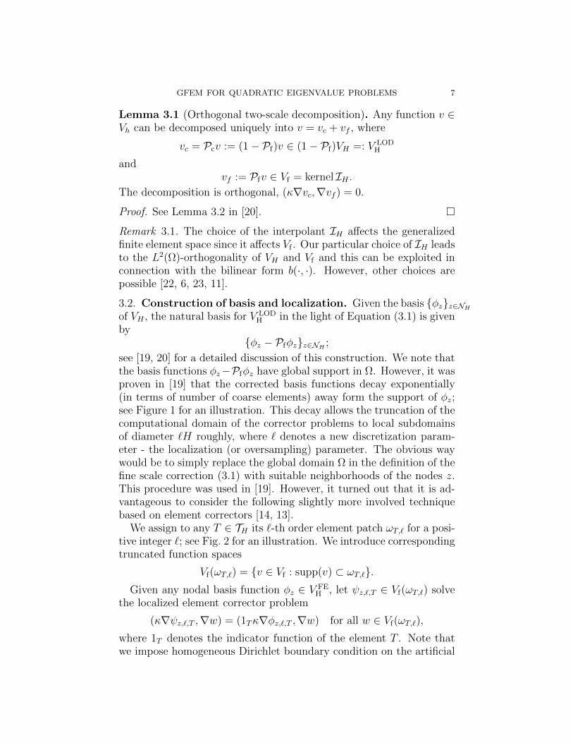
see [19, 20] for a detailed discussion of this construction. We note thatthe basis functions φz−Pfφz have global support in Ω. However, it wasproven in [19] that the corrected basis functions decay exponentially(in terms of number of coarse elements) away form the support of φz;see Figure 1 for an illustration. This decay allows the truncation of thecomputational domain of the corrector problems to local subdomainsof diameter `H roughly, where ` denotes a new discretization param-eter - the localization (or oversampling) parameter. The obvious waywould be to simply replace the global domain Ω in the definition of thefine scale correction (3.1) with suitable neighborhoods of the nodes z.This procedure was used in [19]. However, it turned out that it is ad-vantageous to consider the following slightly more involved techniquebased on element correctors [14, 13].

We assign to any T ∈ TH its `-th order element patch ωT,` for a posi-tive integer `; see Fig. 2 for an illustration. We introduce correspondingtruncated function spaces

Vf(ωT,`) = v ∈ Vf : supp(v) ⊂ ωT,`.Given any nodal basis function φz ∈ V FE

H , let ψz,`,T ∈ Vf(ωT,`) solvethe localized element corrector problem

(κ∇ψz,`,T ,∇w) = (1Tκ∇φz,`,T ,∇w) for all w ∈ Vf(ωT,`),

where 1T denotes the indicator function of the element T . Note thatwe impose homogeneous Dirichlet boundary condition on the artificial


Figure 1. Standard nodal basis function φz with re-spect to the coarse mesh TH (top left), correspondingideal corrector Pfφz (top right), and corresponding cor-rected basis function φz − Pfφz (bottom left). The bot-tom right figure shows a top view on the modulus of thebasis function φz−Pfφz with logarithmic color scale to il-lustrate the exponential decay property. The underlyingrough diffusion coefficient A is depicted in Fig. 4 (left).

boundary of the patch which is well justified by the fast decay. Letψz,` :=

∑T∈TH :z∈T φz,`,T and define the truncated basis function

φz,` := φz − ψz,`.


Figure 2. Element patches ωT,` for ` = 1, 2, 3 (fromleft to right) as they are used in the localized correctorproblem (3.2).

The localized coarse space is then defined as the span of these correctedbasis functions,

V LODH,` := spanφz − ψz,` | z ∈ NH.

Because of the exponential decay of Pfφz the H1(Ω)-error Pfφz − ψz,`can be bounded in terms of Hk (for any k) if ` = C k log(H−1), i.e., ifthe diameter of the patches are of size C kH log(H−1) [19, 20, 14].

3.3. A best approximation result. We will use the approximationproperties of the space V LOD

H,` on several occasions in the error analysisin the next section.

Lemma 3.2. Let m1,m2 : V FEh ×V FE

h → R be bounded bilinear formsand let C, δ1, δ2 ≥ 0 be such that, for all w ∈ V FE

h ,

m1(v, w − IHw) ≤ CHδ1‖v‖‖√κ∇w‖,

m2(v, w − IHw) ≤ CHδ2‖√κ∇v‖‖

√κ∇w‖.

Furthermore, let zj ∈ V FEh (j = 1, 2) solve

(κ∇zj,∇v) = mj(f, v), for all v ∈ V FEh ,

and let zjH,` ∈ V LODH,` solve

(κ∇zjH,`,∇v) = mj(f, v), for all v ∈ V LODH,` ,

with ` = C(δj) log(H−1) chosen appropriately. Then it holds that

‖√κ∇(z1 − z1

H,`‖ ≤ CHδ1‖f‖,‖√κ∇(z2 − z2

H,`‖ ≤ CHδ2‖√κ∇f‖.

Proof. The proof follows from the statement and proof of [19, Theo-rem 4.1] but, for a complete proof, see also in [18, Lemma 3.2]. The


dependency of the constant C(δj) in the relation ` = C(δj) log(H−1) isalso discussed there.

3.4. The proposed method. We are ready to present the approxi-mation of the quadratic eigenvalue problem. Again, we use an operatorformulation based on AH , A

∗H : X → XLOD

H,` = V LODH,` × V LOD

H,` . Given

x ∈ X, AHx ∈ XLODH,` and A∗Hx ∈ XLOD

H,` are characterized by

a(AHx, y) = b(x, y) for all y ∈ XLODH,` ,(3.2)

a(x,A∗Hy) = b(x, y) for all y ∈ XLODH,` .(3.3)

We denote by µiHrHi=1 the eigenvalues of AH that approximate an

eigenvalue µ of the operator A from (2.8). The corresponding invariantsubspace is denoted R(EH). Given a circle ΓH ∈ C in the resolvent setof AH enclosing the eigenvalues µiH

rHi=1, let,

(3.4) EH =1

2πi

∫ΓH

(z − AH)−1 dz.

We note that EH : X → XH is a projection operator, just as itsreference counterpart E defined in (2.10).

3.5. Complexity. Let NH = |NH | be the degrees of freedom in thecoarse finite element mesh TH and Nh = |Nh| the degrees of freedomin the coarse finite element mesh TH . The computation of the mul-tiscale basis V LOD

H,` , using vertex patches of diameter H log(H−1), isproportional to solving NH (independent) Poisson type equations ofsize (Nh log(NH))/NH . Then one quadratic eigenvalue problem of sizeNH need to be solved. Since the convergence rate is typically high (asseen in the numerical experiments) NH can be kept small leading toa very cheap system to solve. This should be compared to solving aquadratic eigenvalue problem of size Nh.

4. Error analysis

In this section we study convergence of the coarse GFE approxima-tion to the discrete reference solution. We shall emphasize that ourerror analysis is fully discrete and does not rely on any regularity as-sumptions on the PDE eigenvalue problem in the limit h → 0. In thepresence of rough coefficients, this will lead to sharp rate. However, forsmoother problems, the worst-case nature of our analysis is presumablya bit pessimistic.

Recall that the space X = V FEh × V FE

h is equipped with the productnorm ‖x‖2

X = ‖√κ∇x1‖2 + ‖x2‖2.


Assumption B. We assume that the bilinear form d associated withthe damping is real and bounded and that there exist C > 0 and0 < γ ≤ 2 such that

(4.1) |d(v, w − IHw)| ≤ CHγ‖∇v‖‖∇w‖ for all v, w ∈ V FEh .

We follow the theory presented in [1], which is in turn based on [21].Note that the constants in the analysis are independent of variationsin κ.

Lemma 4.1. Assumptions (A) and (B) imply

‖A− AH‖X,X ≤ CHmin(1,γ),

‖A∗ − A∗H‖X,X ≤ CHmin(1,γ).

Furthermore,

‖(A− AH)|R(E)‖X,X ≤ CHγ

‖(A∗ − A∗H)|R(E∗)‖X,X ≤ CHγ

Proof. Given x = (x1, x2) ∈ X, y = (y1, y2) = Ax ∈ X satisfies y2 = x1

and

(4.2) (κ∇y1,∇v) = −d(x1, v)− (x2, v) for all v ∈ V FEh .

We let AHx =

[yH1yH2

]where yH2 = Qcx1, Qc being the L2-projection

onto V LODH,` , and yH1 solves,

(4.3) (κ∇yH1 ,∇v) = −d(x1, v)− (x2, v), ∀v ∈ V LODH,` .

We apply Lemma 3.2 twice (with δ1 = γ and δ2 = 1) and conclude

(4.4) ‖∇(y1 − yH1 )‖ ≤ C(Hγ‖√κ∇x1‖+H‖x2‖),

with C > 0 independent of H. Furthermore,

‖y2 − yH2 ‖ = ‖x1 −Qcx1‖ ≤ CH‖∇x1‖.

In summary, for any x ∈ X it holds,

(4.5) ‖(A− AH)x‖X ≤ CHmin(1,γ)‖x‖X .

Similar arguments gives the bound for ‖A∗−A∗H‖X,X . This proves thefirst part of the lemma.

Let µ be an eigenvalue of multiplicity r with corresponding eigen-vector x with components x1

1 and x12. Further let xj1 and xj2 denote the

two components of its generalized eigenfunctions with j ≤ r fulfilling

a(xj, y) = λb(xj, y) + λa(xj−1, y);


see [1, p. 693]. We have that

xj2 =

j−1∑i=1

λixj−i+11 + λj−1x1

1

and also that, for all 2 ≤ j ≤ r,

‖√κ∇xj−1

1 ‖ ≤ C‖√κ∇xj1‖.

Hence,

‖√κ∇xj2‖ ≤ C‖

√κ∇xj1‖.

Applying Lemma 3.2 twice with δ2 = γ and δ2 = 2 and using that(IHx2, vf ) = 0, we get for any x ∈ R(E) with y = Ax and yH = AHxthat

‖√κ∇(y1 − yH1 )‖2

≤ C(Hγ‖√κ∇x1‖+ CH2‖

√κ∇x2‖

)‖√κ∇(y1 − yH1 )‖

≤ C(Hγ +H2)‖√κ∇x1‖‖

√κ∇(y1 − yH1 )‖.

Since γ ≤ 2, we conclude that

(4.6) ‖(A− AH)x‖X ≤ CHγ‖x‖X .

Similar arguments yield the bound for ‖(A∗ − A∗H)|R(E∗)‖X,X .

Lemma 4.1 shows that the approximate operator AH converges innorm, with rate Hmin(1,γ), to A. Therefore also the spectrum con-verges. Given the circle Γ in the complex plane only containing theisolated eigenvalue µ for sufficiently small H the approximate eigen-values µjH will also be inside Γ; see [26]. However, a quantificationof what sufficiently small means is difficult as it depends also on theunknown spectrum and, in particular, the sizes and the separation ofthe eigenvalues. For a given range of coarse discretization parameters,we will, hence, have to assume that a curve Γ exists that contains onlyµ and µjH , j = 1, . . . , r, or expressed in an other way, that the curveΓH in Equation (3.4) may be chosen equal to Γ.Assumption C. Given h and an eigenvalue µ, we assume that thereexists H0 > h such that for all h ≤ H ≤ H0 the curve ΓH in Equa-tion (3.4) only containing the eigenvalues µjH , j = 1, . . . , r can be chosenequal to Γ which contains only µ.

We will comment further on this assumption in the numerical exam-ples. For the subsequent error analysis it means that the results areonly valid in the regime h ≤ H ≤ H0.


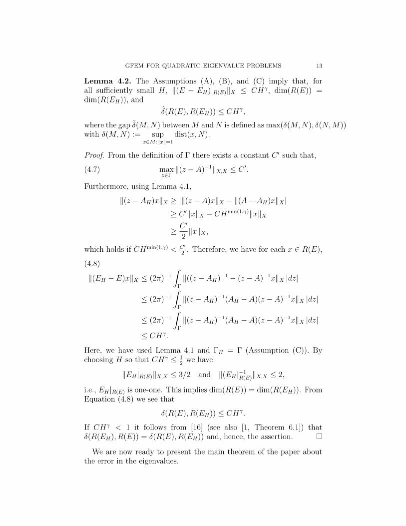
Lemma 4.2. The Assumptions (A), (B), and (C) imply that, forall sufficiently small H, ‖(E − EH)|R(E)‖X ≤ CHγ, dim(R(E)) =dim(R(EH)), and

δ(R(E), R(EH)) ≤ CHγ,

where the gap δ(M,N) betweenM andN is defined as max(δ(M,N), δ(N,M))with δ(M,N) := sup

x∈M :‖x‖=1

dist(x,N).

Proof. From the definition of Γ there exists a constant C ′ such that,

(4.7) maxz∈Γ‖(z − A)−1‖X,X ≤ C ′.

Furthermore, using Lemma 4.1,

‖(z − AH)x‖X ≥ |‖(z − A)x‖X − ‖(A− AH)x‖X |≥ C ′‖x‖X − CHmin(1,γ)‖x‖X

≥ C ′

2‖x‖X ,

which holds if CHmin(1,γ) < C′

2. Therefore, we have for each x ∈ R(E),

‖(EH − E)x‖X ≤ (2π)−1

∫Γ

‖((z − AH)−1 − (z − A)−1x‖X |dz|

(4.8)

≤ (2π)−1

∫Γ

‖(z − AH)−1(AH − A)(z − A)−1x‖X |dz|

≤ (2π)−1

∫Γ

‖(z − AH)−1(AH − A)(z − A)−1x‖X |dz|

≤ CHγ.

Here, we have used Lemma 4.1 and ΓH = Γ (Assumption (C)). Bychoosing H so that CHγ ≤ 1

2we have

‖EH |R(E)‖X,X ≤ 3/2 and ‖(EH |−1R(E)‖X,X ≤ 2,

i.e., EH |R(E) is one-one. This implies dim(R(E)) = dim(R(EH)). FromEquation (4.8) we see that

δ(R(E), R(EH)) ≤ CHγ.

If CHγ < 1 it follows from [16] (see also [1, Theorem 6.1]) thatδ(R(EH), R(E)) = δ(R(E), R(EH)) and, hence, the assertion.

We are now ready to present the main theorem of the paper aboutthe error in the eigenvalues.


Theorem 4.3. Let µ be an isolated eigenvalue of A of algebraic multi-plicity r and ascent α, with associate invariant subspace R(E). Underassumption (A), (B), and (C), for sufficiently small H it holds,

(4.9) |µ− µjH | ≤ CH2γα , j = 1, . . . , r.

Proof. Let φiri=1 span R(E) and φ∗i ri=1 span R(E∗), both normal-ized in L2(Ω). Lemma 4.2 is valid and therefore Theorem 7.3 in [1]gives,

|µ− µjH |α ≤ C

r∑i,j=1

|a(A− AH)φi, φ∗j)|

+ C‖(A− AH)|R(E)‖X,X‖(A∗ − A∗H)|R(E∗)‖X,X .The second term has been bounded in Lemma 4.1. The first term

remains. Using Galerkin Orthogonality we can subtract any y ∈ XLODH,`

in the right slot. Using Lemmas 4.1 we get,

a((A− AH)φi, φ∗j) ≤ ‖(A− AH)|R(E)‖X,X inf

z∈XLODH,`

supx∈R(E∗)

‖x− z‖X

≤ CHγ infz∈XLOD

H,`

supx∈R(E∗)

‖x− z‖X .

Here Lemma 3.2 applies with δ2 = γ. We also note that similar to theproof of the second part of Lemma 4.1 we have ‖

√κ∇x2‖ ≤ C‖

√κ∇x1‖

for xj ∈ R(E∗) and therefore,

infz∈XLOD

H

supx∈R(E∗)

‖x− z‖X ≤ CHγ.

The theorem follows.

Remark 4.1. The theorem states a similar result as Theorem 8.3 in [1]but for this specific method. Also a result similar to Theorem 8.2 in[1] can be derived in the same way. It holds,∣∣∣∣∣∣µ−1 −

(1

r

r∑j=1

µjH

)−1∣∣∣∣∣∣ ≤ CH2γ.

5. Numerical Experiments

In all subsequent experiments, we let Ω = [0, 1]2 and we considernested uniform rectangular triangulations (as depicted in Figure 3)on all scales. The fine reference scale will be fixed throughout bythe choice h = 2−8.5. The coarse mesh size will typically varies,H = 2−1.5, 2−2.5, 2−3.5, 2−4.5, 2−5.5. The corresponding finite elementspaces are V FEM

H ⊂ V FEMh . For each of these spaces we construct the


Figure 3. Uniform triangulations of the unit squarewith H = 2−0.5, 2−1.5 as they are used in the numericalexperiments.

Figure 4. Coefficients in the numerical experiments ofSection 5.1. Left: Constant diffusion coefficient. Mid-dle: Rapidly varying diffusion diffusion. Right: Weightfunction for mass-type damping.

corresponding LOD spaces V LODH,` with a certain choice of the localiza-

tion parameter `. Throughout the numerical experiments, we plot therelative error for the eight smallest (magnitude) eigenvalues. For thesolution of the algebraic eigenvalue problems, we use the MATLABbuilt-in eigenvalue solver eigs with tolerance 1e-10.

5.1. Smooth mass-type damping. We consider damping by a mod-ified mass matrix associated with the bilinear form

(5.1) d(v, w) =

∫Ω

(1 + sin(10x1))v(x1, x2)w(x1, x2) d(x1, x2).

Clearly,

|d(v, w − IHw)| ≤ CH2‖√κ∇v‖‖

√κ∇w‖,

i.e., Assumption (B) holds with γ = 2.To begin with, let κ = 1. Figure 5 shows the convergence rate of the

8 smallest (complex conjugate) eigenvalues as a function of the coarsemesh size. We observe a convergence rate of H6 which is more thanwe expect from the theory (H2γ = H4 for simple eigenvalues). This


10-1

10-10

10-8

10-6

10-4

10-2

100

λ1,λ

2

λ3,λ

4

λ5,λ

6

λ7,λ

8

H2

H4

H6

-0.8 -0.7 -0.6 -0.5 -0.4-10

-8

-6

-4

-2

0

2

4

6

8

10

exact

H=2-1.5

H=2-2.5

H=2-3.5

H=2-4.5

H=2-5.5

Figure 5. First numerical experiment in Section 5.1 forconstant diffusion and smooth damping weight depictedin Fig. 4 (left and right). Left: Relative eigenvalue er-rors vs. coarse mesh size H with localization parameter` = d3 log(H−1)e. Right: Illustration of eigenvalue con-vergence as H decreases.

may be related to the high regularity of the underlying PDE eigenvalueproblem which we do not take advantage of in the analysis.

In the second numerical example we let κ be a piecewise constantfunction on a 64×64 uniform grid depicted in Figure 4. In every squareelement we pick on value from the uniform distribution U([0.003, 1]).This gives a deterministic rapidly varying diffusion coefficient with as-pect ratio over 300, see Figure 4 (middle). We keep the rest of thesetup the same, i.e., d is still chosen as in Equation (5.1). In Figure 6,we see that we get the H4 convergence as predicted by the theory. Thesame convergence rate was also detected for the corresponding lineareigenvalue problem in [20].

5.2. Discontinuous mass-type damping with composite mate-rial configuration. We now consider a situation where κ jumps be-tween two values in the domain, namely,

κ =

1 in Ω1,α in Ω \ Ω1.

This models a composite with two different materials. We pick thedomain Ω to be the union of a periodic array of square inclusion asdepicted in Figure 8 (left). We assume that the damping has the same


10-1

10-8

10-6

10-4

10-2

100

λ1,λ

2

λ3,λ

4

λ5,λ

6

λ7,λ

8

H2

H4

H6

-0.8 -0.7 -0.6 -0.5 -0.4

-6

-4

-2

0

2

4

6

exact

H=2-1.5

H=2-2.5

H=2-3.5

H=2-4.5

H=2-5.5

Figure 6. Second numerical experiment in Section 5.1for rough diffusion and smooth damping weight depictedin Fig. 4 (middle and right). Left: Relative eigenvalueerrors vs. coarse mesh size H with localization param-eter ` = d3 log(H−1)e. Right: Illustration of eigenvalueconvergence as H decreases.

Figure 7. Coefficients in the numerical experiments ofSections 5.2–5.3. Left: Discontinuous diffusion coeffi-cient. Middle: Discontinuous weight function for mass-type damping. Right: Discontinuous weight function forstiffness-type damping.

structure represented by the coefficient

κ =

β in Ω1,µ in Ω \ Ω1,

and we study mass type damping represented by the κ-weighted L2

scalar product

d(v, w) = (κv, w).


10-1

10-8

10-6

10-4

10-2

100

λ1,λ

2

λ3,λ

4

λ5,λ

6

λ7,λ

8

H2

H4

H6

-0.19 -0.185 -0.18 -0.175-4

-3

-2

-1

0

1

2

3

4

exact

H=2-1.5

H=2-2.5

H=2-3.5

H=2-4.5

H=2-5.5

Figure 8. Numerical experiment in Section 5.2 for dis-continuous diffusion and discontinuous mass-type damp-ing depicted in Fig. 7 (left and middle). Left: Relativeeigenvalue errors vs. coarse mesh size H with localiza-tion parameter ` = d3 log(H−1)e. Right: Illustration ofeigenvalue convergence as H decreases. Note that theeigenvalues λ3, λ5 (resp. λ4, λ6) are clustered and canhardly be distinguished in the plot.

Note that in this case,

d(v, w − IHw) ≤ CH‖v‖‖√κ∇w‖,

i.e., γ = 1. Hence, our theory predicts only convergence of order H2.We can not immediately get a higher rate since κ is not differentiable.We let α = µ = 0.1 and β = 1.1. This is an academic choice usedto test the numerical methods presented in the paper. Figure 8 showsthe convergence of the error as the dimension of the coarse multiscalespace depending on the coarse mesh size. The rate increases with thesize of the system and we still observe H4 convergence.

In the error analysis, we have assumed that the eigenvalues areisolated and that the approximate eigenvalues are found in a neigh-borhood of the exact ones. This was formulated in Assumption (C)above. While this assumption could be verified a posteriori in theprevious experiments with semi-simple and well-separated eigenvalues(cf. Figures 5(right), 6(right)), we now observe clustered eigenvalues


10-1

10-3

10-2

10-1

λ1,λ

2

λ3,λ

4

λ5,λ

6

λ7,λ

8

0.1H4/3

-0.8 -0.6 -0.4 -0.2-4

-3

-2

-1

0

1

2

3

4

exact

H=2-1.5

H=2-2.5

H=2-3.5

H=2-4.5

H=2-5.5

Figure 9. Numerical experiment in Section 5.3 for dis-continuous diffusion and discontinuous mass-type damp-ing depicted in Fig. 7 (left and right). Left: Relativeeigenvalue errors vs. coarse mesh size H with localiza-tion parameter ` = d2 log(H−1)e. Right: Illustration ofeigenvalue convergence as H decreases. Note that theeigenvalues λ3, λ5 (resp. λ4, λ6) are clustered and canhardly be distinguished in the plot.

and the violation of Assumption (C) on the coarsest meshes (cf. Fig-ure (8)(right)). Still, the quality of the approximate spectrum is com-parable to the previous experiments.

5.3. Discontinuous stiffness-type damping. Now we consider stiff-ness type damping,

d(v, w) = (κ∇v,∇w).

We let α = 0.1, µ = 0.015, and β = 0.006. In Figure 9, we seethe convergence of the error as the coarse mesh size decreases. Theparameter γ in Assumption (B) is equal to zero for discontinuous κso that the theory does not predict any rate of convergence. Still, wedetect O(H4/3) convergence roughly with pre-asymptotic effects onlyon the coarsest grid. Again, this may be related to the regularity of theunderlying PDE eigenvalue problem which we do not take advantageof in the analysis.


6. Conclusion

We present an efficient numerical procedure applicable for a class ofquadratic eigenvalue problems, discretized using conforming P1 finiteelements. The main idea is to construct a low dimensional subspace ofthe finite element space that capture crucial features of the problem.In particular we consider problems with rapid data variation, model-ing for instance composite materials. The numerical results are verypromising. High convergence rates without pre-asymptotic regime aredetected. This indicates that already low dimensional GFEM spacesgive sufficient accuracy in the eigenvalue approximation. Therefore,the task of solving a very large quadratic eigenvalue problem can bereplaced by the task of solving of many localized independent linearPoisson type problems followed by one small quadratic eigenvalue prob-lem. This conclusion was also made for linear eigenvalue problems in[20] and eigenvalue problems involving a non-linearity in the eigenfunc-tion [12].

In the error analysis, we prove convergence with rate for the eigen-values and eigenspaces. The result are based on classical works fornon-symmetric eigenvalue problems nicely summarized in [1] and re-cent work of the authors for linear eigenvalue problems. The resultsrely on qualitative assumptions on the size of H and the distribution ofthe discrete and exact eigenvalues. Without explicit knowledge on thestructure of the damping, it seems to be difficult to avoid them or re-place them with more quantitative assumptions. However we have notyet observed any problems in the numerical experiments. A challengefor future research would be to rigorously justify the numerical perfor-mance in the targeted pre-asymptotic regime, at least for practicallyrelevant classes of damping.

References

[1] I. Babuska and J. Osborn, Eigenvalue problems. In Handbook of numericalanalysis, Vol. II, Handb. Numer. Anal., II, 641–787. North-Holland, Amster-dam, 1991.

[2] I. Babuska and J. Osborn, Can a finite element method perform arbitrarybadly?, Math. Comp., 69 (1999), 443–462.

[3] A. Bermudez, R. G. Duran, R. Rodrıguez, and J. Solomin, Finite element anal-ysis of a quadratic eigenvalue problem arising in dissipative acoustics, SIAMJ. Numer. Anal., 38 (2000), 267–291.

[4] T. Betcke, N. Higham, V. Mehrmann, and C. Schroder, NLEVP: A Collec-tion of Nonlinear Eigenvalue Problems, ACM Transactions on MathematicalSoftware, 39 (2013), 7:1–7:28.

[5] D. Boffi, Finite element approximation of eigenvalue problems, Acta Numer.,19:1–120, 2010.


[6] D. Brown and D. Peterseim. A multiscale method for porous microstructures.ArXiv e-prints, November 2014.

[7] C. Carstensen and R. Verfurth, Edge residuals dominate a posteriori errorestimates for low order finite element methods, SIAM J. Numer. Anal. 36(1999), 1571–1587.

[8] P. G. Ciarlet, The finite element method for elliptic problems, Classics in Ap-plied Mathematics, 40, SIAM, Philadelphia, 2002.

[9] J. Descloux, N. Nassif, and J. Rappaz, On spectral approximation. Part 1: Theproblem of convergence, RAIRO Anal. Numer., 12 (1978), 97–112.

[10] J. Descloux, N. Nassif, and J. Rappaz, On spectral approximation. Part 2:Error estimates for the Galerkin method, RAIRO Anal. Numer., 12 (1978),113–119.

[11] D. Gallistl and D. Peterseim, Stable multiscale Petrov-Galerkin finite elementmethod for high frequency acoustic scattering, Comp. Meth. Appl. Mech. Eng.,295 (2015), 1–17.

[12] P. Henning, A. Malqvist, and D. Peterseim, Two-level discretization techniquesfor ground state computations of Bose-Einstein condensates, SIAM J. Nu-mer. Anal.,52 (2014), 1525–1550.

[13] P. Henning, P. Morgenstern, and D. Peterseim. Multiscale partition of unity.In Michael Griebel and Marc Alexander Schweitzer, editors, Meshfree Methodsfor Partial Differential Equations VII, volume 100 of Lecture Notes in Compu-tational Science and Engineering, pages 185–204. Springer International Pub-lishing, 2015.

[14] P. Henning and D. Peterseim. Oversampling for the multiscale finite elementmethod. Multiscale Modeling & Simulation, 11(4):1149–1175, 2013.

[15] T.-M. Hwang, W.-W. Lin, and V: Mehrmann, Numerical solution of quadraticeigenvalue problems with structure-perserving methods, SIAM J. Sci. Comp.,24 (2003), 1283–1302.

[16] T. Kato, Perturbation theory for linear operators, Springer-Verlag, New York,1976.

[17] V. Mehrmann and H. Voss, Nonlinear eigenvalue problems: a challenge formodern eigenvalue methods, GAMM-Mitt., 27 (2004), 121–152.

[18] A. Malqvist and A. Persson, Multiscale techniques for parabolic equations,arXiv/1504.08140v1

[19] A. Malqvist and D. Peterseim, Localization of elliptic multiscale problems,Math. Comp., 83 (2014), 2583–2603.

[20] A. Malqvist and D. Peterseim, Computation of eigenvalues by numerical up-scaling, Numer. Math., 130 (2015), 337–361.

[21] J. E. Osborn, Spectral approximation for compact operators, Math. Comp., 29(1975), 712–725.

[22] D. Peterseim. Eliminating the pollution effect in Helmholtz problems by localsubscale correction. ArXiv e-prints, 1411.1944, 2014.

[23] D. Peterseim, Variational multiscale stabilization and the exponential decay offine-scale correctors, ArXiv e-prints, May 2015.

[24] G. Strang and G. Fix, An analysis of the finite element method,[25] F. Tisseur and K. Meerbergen, A Survey of the Quadratic Eigenvalue Problem,

SIAM Review, 43, (2001) 235–286.


[26] J. Weidmann, Strong operator convergence and spectral theory of ordinary dif-ferential operators, Univ. Iagel. Acta Math., 34 (1997), 153–163.

Department of Mathematics, Chalmers University of Technologyand University of Gothenburg

Insitute for Numerical Simulation, Rheinische Friedrich-Wilhelms-Universitat Bonn

generalizedﬁniteelementmethods forquadraticeigenvalueproblems · mis the mass matrix, is the...

Documents