calculation of eigenvalue and eigenvector derivatives with...

Structural Engineering and Mechanics, Vol. 36, No. 1 (2010) 37-55 37

Calculation of eigenvalue and eigenvector derivatives with the improved Kron’s substructuring method

*Yong Xia1, Shun Weng1a, You-Lin Xu1b and Hong-Ping Zhu2c

1Department of Civil & Structural Engineering, The Hong Kong Polytechnic University,

Hung Hom, Kowloon, Hong Kong2School of Civil Engineering & Mechanics, Huazhong University of Science and Technology,

Wuhan, Hubei, P.R. China

(Received August 31, 2009, Accepted April 20, 2010)

Abstract. For large-scale structures, the calculation of the eigensolution and the eigensensitivity isusually very time-consuming. This paper develops the Kron’s substructuring method to compute the first-order derivatives of the eigenvalues and eigenvectors with respect to the structural parameters. The globalstructure is divided into several substructures. The eigensensitivity of the substructures are calculated viathe conventional manner, and then assembled into the eigensensitivity of the global structure byperforming some constraints on the derivative matrices of the substructures. With the proposedsubstructuring method, the eigenvalue and eigenvector derivatives with respect to an elemental parameterare computed within the substructure solely which contains the element, while the derivative matrices ofall other substructures with respect to the parameter are zero. Consequently this can reduce thecomputation cost significantly. The proposed substructuring method is applied to the GARTEUR AG-11frame and a highway bridge, which is proved to be computationally efficient and accurate for calculationof the eigensensitivity. The influence of the master modes and the division formations are also discussed.

Keywords: substructuring method; eigensolution; eigensensitivity; model updating.

1. Introduction

Finite element (FE) model updating technology has been extensively developed in aerospace,

mechanical and civil engineering. It can serve for structural modification, model tuning, and damage

identification (Friswell 1995). Model updating methods are usually classified into one-step methods

and iterative methods (Brownjohn 2001). The one-step methods directly reconstruct the global

stiffness matrix and the mass matrix, while the iterative methods modify the physical parameters in

the FE model iteratively to realize an optimal match between the analytical modal properties (such

as the frequencies and the modal shapes) and the measurements. The latter approach has been

becoming more popular because they allow physical meaning of the obtained modifications and can

*Corresponding author, Assistant Professor, E-mail: [email protected]. D Student, E-mail: [email protected] Professor, E-mail: [email protected], E-mail: [email protected]

38 Yong Xia, Shun Weng, You-Lin Xu and Hong-Ping Zhu

preserve the symmetry, the positive-definiteness and the sparseness in the updated matrices.

However, one drawback of the iterative methods lies in that the eigensolutions of the analytical

model and their associated sensitivity matrices usually need to be calculated in each iteration (Bakir

2007).

Eigensensitivity is usually calculated in the global structure level. Fox and Kapoor (1968) firstly

utilized the modal method to determine the eigenvalue and eigenvector derivatives by considering

the changes of the physical parameters in the mass and stiffness matrices. The disadvantage of this

method lies in that all modes of the system are required, which is computationally expensive for

large-scale structures. Nelson (1976) proposed a more efficient method to calculate the eigenvector

derivatives by using the modal parameters of that mode solely. Lin et al. (1995, 1996b) further

improved the computation efficiency of the Nelson’s method, by combining the inverse iteration

technique, the singular value decomposition theory and the model reduction technique. The Nelson’s

method has also been developed to treat with the rigid body modes, the close or repeated modes by

some researchers (Lin 1996a, Song 1996, Wu 2007).

Since calculation of the eigensensitivity usually dominants computation time during the iterative

model updating process, how to calculate the eigensensitivity efficiently becomes a big challenge

for the researchers. The substructuring technology can be a promising solution to accelerate the

calculation of the eigensensitivity for large-scale structures. In general, the substructuring methods

include three steps: first, the global structure is torn into some manageable substructures according

to some division criteria; second, the substructures are analyzed independently to obtain the

designated solutions (for example, the eigenpairs and eigensolution derivatives); finally, the

solutions of the substructures are assembled to obtain the properties of the global structure by

imposing constraints on the interface of the adjacent substructures (Yun et al. 1997). With the

substructuring method, the eigensolutions and the eigensensitivity of the modified substructures are

repeatedly analyzed, while the unmodified substructures are unchanged during the iterative model

updating process. In addition, the substructuring method is expected to be more efficient when it is

incorporated with the parallel computation (Fulton 1991) or the model reduction techniques

(Choi et al. 2008, Xia and Lin 2004).

Hurty (1965) and Craig-Bampton (1968, 2000) developed a substructuring method based on the

constraint modes with the fixed-interface condition of the substructures, while MacNeal (1971) and

Rubin (1975) proposed a substructuring method based on the attachment modes with the free-

interface condition. Qiu (1997) expressed the displacement of the substructures with the

combination of the fixed interface modes and the free interface modes. Based on the different

boundary conditions, Heo and Ehmann (1991) and Lallemand et al. (1999) derived the

eigensolution derivatives by using the fixed-interface substructuring method and the free-interface

substructuring method, respectively. The constraint modes or the linked force are required

beforehand to construct the eigensensitivity formula. Gabriel Kron (1968) initiated a substructuring

method to study the eigensolutions of the systems with large number of variables in a piece-wise

manner. The Kron’s method has a concise form, and has been developed by a few researchers

(Simpson 1973, Simpson and Tabarrok 1968, Sehmi 1986). Recently, the Weng and Xia (2007)

proposed a modal truncation technique to transform the original Kron’s substructuring eigenequation

into a simplified form, and improved the computation efficiency of the Kron’s substructuring

method. Only some lower eigenmodes of the substructures are retained as the master modes in the

technique, while the higher modes are discarded and compensated with the residual flexibility. The

method can achieve high precision with the second-order residual flexibility, or even high-order

Calculation of eigenvalue and eigenvector derivatives 39

residual flexibility.

The improved Kron’s substructuring method is extended in this paper, to derive the first-order

derivatives of the eigensolutions with respect to a structural parameter. With the proposed

substructuring method, the derivatives matrices of the eigensolutions and the residual flexibility with

respect to the elemental parameter are computed within a particular substructure, while the

derivative matrices of the other substructures are zero. The eigensensitivity of the global structure

with respect to the elemental parameter is recovered from the derivative matrices of the particular

substructure. Since the residual flexibility is symmetric and directly related to the stiffness matrix,

the first-order and high-order eigensensitivity can be calculated by directly re-differentiating the

eigenequation with respect to the structural parameter. To verify the effectiveness and the accuracy

of the proposed technique, the eigensensitivity formula is applied into the GARTEUR AG-11

structure and a highway bridge.

2. Basic theory

Generally, the global structure with N degree of freedoms (DOFs) is firstly divided into NS

independent substructures. The jth (j = 1, 2, …, NS) substructure with n(j) DOFs has the sub-

matrices and , and the associated n(j) eigenpairs as

,

, (1)

The eigensolutions of the substructures are diagonally assembled into the primitive form as

, (2)

Hereinafter, the superscript ‘p’ represents the primitive matrices, which are diagonally assembled

from the substructures directly. The divided substructures are then reconnected by the virtual work

principle and the geometric compatibility. Kron’s substructuring method makes full use of the

orthogonality properties, and transforms the eigenequation of the assembled global structure into

(Sehmi 1986)

(3)

in which , and C is a rectangular connection matrix, which constraints the interface

DOFs to move jointly (Sehmi 1986, Turner 1983). In C matrix, each row contains two non-zero

elements. For rigid connections the two elements will be 1 and −1. If the connected points x1 and x2

are not rigidly connected, which has the relationship , the two elements in the

corresponding row of matrix C will be 1 and −r. Kron’s substructuring method considers the

connection condition by the matrix C, and has a concise form (Turner 1983). τ is the internal

connection forces; is the eigenvalue of the global structure; z is regarded as the mode

participation factor, which indicates the contribution of the eigenmodes of the substructures to the

Kj( )

Mj( )

Λj( )

Diag λ1

j( )λ2

j( ) … λn

j( )

j( ), , ,[ ]= Φj( )

φ 1

j( )φ 2

j( ) … φn

j( )

j( ), , ,[ ]=

Φj( )[ ]

TK

j( )Φ

j( )Λ

j( )= Φ

j( )[ ]TM

j( )Φ

j( )I

j( )=

Λp

Diag Λ1( )Λ

2( ) … ΛNS( ), , ,[ ]= Φ

pDiag Φ

1( )Φ

2( ) … ΦNS( ), , ,[ ]=

Λp

λI – Γ–

Γ–T

0

z

τ⎩ ⎭⎨ ⎬⎧ ⎫ 0

0⎩ ⎭⎨ ⎬⎧ ⎫

=

Γ CΦp[ ]

T=

x1 rx2=

λ


eigenmodes of the global structure. The eigenvectors of the global structure Φ can be recovered by

and removing the identical elements of at the interfaces.

In Eq. (2), the primitive matrices and require calculating the complete eigensolutions

of all substructures, which is time-consuming. The complete modes of each substructure are

partitioned into the master part and the slave part (Weng et al. 2009). The first a few eigenmodes in

each substructure are retained as the ‘master’ modes, while the residual higher eigenmodes are

discarded as the ‘slave’ modes and compensated by the first-order residual flexibility. Assuming that

the subscript ‘m’ and ‘s’ represents the ‘master’ and ‘slave’ variables respectively, the jth

substructure has m(j) ‘master’ eigenpairs and s(j) ‘slave’ eigenpairs as

,

, (4)

Assembling the master eigenpairs and the slave eigenpairs respectively, one has

,

,

,

, , , (5)

Partitioning Eq. (3) according to the master and slave modes, Eq. (3) can be expanded as

(6)

The second line of Eq. (6) gives

(7)

Substituting Eq. (7) into Eq. (6) results in

(8)

The interested eigenvalues correspond to the lowest modes of the global structure, and are far

less than the items in when the master modes are properly chosen. Eq. (8) is approximated as

Φ Φp

z{ }= Φ

Λp[ ] Φ

p[ ]

Λm

j( )Diag λ1

j( )λ2

j( ) … λm

j( )

j( ), , ,[ ]= Φm

j( )φ 1

j( )φ 2

j( ) … φm

j( )

j( ), , ,[ ]=

Λs

j( )Diag λ

mj( )

1+

j( )λm

j( )2+

j( ) … λm

j( )s

j( )+

j( ), , ,[ ]= Φs

j( )φm

j( )1+

j( )φm

j( )2+

j( ) … φm

j( )s

j( )+

j( ), , ,[ ]=

Λm

pDiag Λm

1( )Λm

2( ) … Λm

NS( ), , ,[ ]= Φm

pDiag Φm

1( )Φm

2( ) … Φm

NS( ), , ,[ ]=

Λs

pDiag Λs

1( )Λs

2( ) … Λs

NS( ), , ,[ ]= Φs

pDiag Φs

1( )Φs

2( ) … Φs

NS( ), , ,[ ]=

Γm CΦm

p[ ]T

= Γs CΦs

p[ ]T

=

mp

mj( )

j 1=

NS

∑= sp

sj( )

j 1=

NS

∑= mj( )

sj( )

+ nj( )

= j 1 2 … NS, , ,=( )

Λm

pλI – 0 Γm–

0 Λs

pλI – Γs–

Γm

T– Γs

T– 0

zm

zs

τ⎩ ⎭⎪ ⎪⎨ ⎬⎪ ⎪⎧ ⎫ 0

0

0⎩ ⎭⎪ ⎪⎨ ⎬⎪ ⎪⎧ ⎫

=

zs Λs

pλI–( )

1–

Γsτ=

Λm

pλI – Γm–

Γm

T– Γs

TΛs

pλI–( )

1–

Γs–

zm

τ⎩ ⎭⎨ ⎬⎧ ⎫ 0

0⎩ ⎭⎨ ⎬⎧ ⎫

=

λ

Λs

p


(9)

Representing τ with zm from the second line of Eq. (9) and substituting it into the first line, the

eigenequation is simplified into

(10)

(11)

where is the first-order residual flexibility, which is represented by diagonally

assembling the stiffness matrices and the master modes of the substructures as

(12)

In Eq. (10), the mode participation factor leads to the eigenvectors of the global structure

via the transform of . The reduced eigenequation (Eq. (10)) has the size of mp, which

is much smaller than that of the original one (Eq. (3)).

3. Eigenvalue derivatives with the substructuring method

For the ith mode, the eigenequation (Eq. (10)) can be rewritten as

(13)

Eq. (13) is differentiated with respect to a design parameter r as

(14)

Pre-multiplying on both sides of Eq. (14) gives

(15)

Due to symmetry of , the first item in the left hand side of

Eq. (15) is zero. Arranging Eq. (15), the derivative of the eigenvalue with respect to the design

parameter r is

(16)

Λm

pλI – Γm–

Γm

T– Γs

TΛs

p( )1–

Γs–

zm

τ⎩ ⎭⎨ ⎬⎧ ⎫ 0

0⎩ ⎭⎨ ⎬⎧ ⎫

=

Λm

pΓm Γs

TΛs

p( )1–

Γs( )1–

Γm

T+[ ] zm{ } λ zm{ }=

Γs

TΛs

p( )1–

Γs CΦs

pΛs

p( )1–

Φs

p[ ]TC

T=

Φs

pΛs

p( )1–

Φs

p[ ]T

Φs

pΛs

p( )1–

Φs

p[ ]T

Diag K1( )( )

1–

Φm

1( )Λm

1( )( )1–

Φm

1( )[ ]T

–( ) … KNS( )( )

1–

Φm

NS( )Λm

NS( )( )1–

Φm

NS( )[ ]T

–( ), ,[ ]=

zm{ }Φ Φm

pzm{ }=

Λm

pΓm Γs

TΛs

p( )1–

Γs( )1–

Γm

T+[ ] zi{ } λi zi{ }=

Λm

pΓm Γs

TΛs

p( )1–

Γs( )1–

Γm

TλiI–+[ ]

∂zi

∂r-------

⎩ ⎭⎨ ⎬⎧ ⎫ ∂ Λm

pΓm Γs

TΛs

p( )1–

Γs( )1–

Γm

TλiI–+[ ]

∂r--------------------------------------------------------------------------------- zi{ }+ 0{ }=

zi{ }T

zi{ }T Λm

pΓm Γs

TΛs

p( )1–

Γs( )1–

Γm

TλiI–+[ ]

∂zi

∂r------

⎩ ⎭⎨ ⎬⎧ ⎫

zi{ }T∂ Λm

pΓm Γs

TΛs

p( )1–

Γs( )1–

Γm

TλiI–+[ ]

∂r------------------------------------------------------------------------------ zi{ }+ 0=

Λm

pΓm Γs

TΛs

p( )1–

Γs( )1–

Γm

TλiI–+[ ]

λi

∂λi

∂r------- zi{ }T

∂ Λm

pΓm Γs

TΛs

p( )1–

Γs( )1–

Γm

T+[ ]

∂r--------------------------------------------------------------------- zi{ }=


in which

In Eq. (16), is the diagonal assembly of the eigenvalue derivatives of the substructures,

and is associated with the diagonal assembly of the eigenvector derivatives of the

substructures. is the derivative matrix of the first-order residual flexibility of

the substructures.

Since the substructures are independent, the derivative matrices of the eigenvalues, the

eigenvectors and the residual flexibility are only calculated in the particular substructure (for

example, the rth substructure) which contains the elemental parameter r. These quantities in other

substructures are zero. Within the rth substructure, the eigenvalue and eigenvector derivatives can

be obtained by the traditional methods, such as Nelson’s method (Nelson 1976). The derivative of

the residual flexibility with respective to the structural parameter r is

(17)

and

(18)

It is noted that, if the substructure (for example, the jth substructure) is free, the stiffness matrix

is singular, and the inversion of to form the residual flexibility does not exist.

Consequently, the derivative of the residual flexibility of the free-free substructure is not available.

In this situation, the rigid body modes, which contribute to the zero-frequency modes, are employed

(Felippa et al. 1998). The detailed procedures on how to calculate the residual flexibility and the

first-order derivatives of the free-free substructures can be found in Appendix.

It is noted that the eigenvalue derivatives of the global structure with respect to an elemental

parameter solely rely on the particular substructure (the rth substructure) rather than the other

∂ Λm

pΓm Γs

TΛs

p( )1–

Γs( )1–

Γm

T+[ ]

∂r---------------------------------------------------------------------

∂Λm

p

∂r----------

∂Γm

∂r--------- Γs

TΛs

p( )1–

Γs( )1–

Γm

TΓm

∂ Γs

TΛs

p( )1–

Γs( )1–

[ ]∂r

-------------------------------------------Γm

TΓm Γs

TΛs

p( )1–

Γs( )1– ∂Γm

T

∂r---------+ + +=

∂Λm

p/∂r

∂Γm

∂r---------

∂ Φm

p[ ]T

∂r-----------------C

T=

∂ Γs

TΛs

p( ) 1–

Γs( )1–

[ ]/∂r

∂ Γs

TΛs

p( )1–

Γs( )1–

∂r-------------------------------------- Γs

TΛs

p( )1–

Γs( )1– ∂ Γs

TΛs

p( )1–

Γs( )∂r

---------------------------------- Γs

TΛs

p( )1–

Γs( )1–

=

∂ Γs

TΛs

p( )1–

Γs( )∂r

--------------------------------- C∂ Φs

pΛs

p( )1–

Φs

p[ ]T

( )∂r

------------------------------------------CT

C Diag

0

∂ Kr( )( )

1–

Φm

r( )Λm

r( )( )1–

– Φm

r( )[ ]T

( )∂r

-----------------------------------------------------------------------

0

CT××==

C Diag

0

∂ Kr( )( )

1–

∂r--------------------

∂Φm

r( )

∂r------------ Λm

r( )( )1–

Φm

r( )[ ]T

– Φm

r( )Λm

r( )( )1– ∂Λm

r( )

∂r----------- Λm

r( )( )1–

Φm

r( )[ ]T

Φm

r( )Λm

r( )( )1– ∂ Φm

r( )[ ]T

∂r------------------–+

0

CT××=

Kj( )

Kj( )


substructures. Since the size of the substructures is always smaller than that of the global structure,

the computation efficiency is improved. This significant merit might be very attractive when it is

applied to the iterative model updating. With the substructuring method, only the modified

substructures are re-analyzed, while other substructures are untouched. In addition, due to the

symmetric and simple form of the residual flexibility, there is no difficulty to derive the high-order

derivatives of the eigenvalues by directly differentiating the eigensensitivity equation (Eq. (16)),

which needs to calculate the eigenvector derivatives first.

4. Eigenvector derivatives with the substructuring method

Since the ith eigenvector of the global structure can be recovered by

(19)

the eigenvector derivative of the ith mode with respect to the structural parameter r can be

differentiated as

(20)

In Eq. (20), are the eigenvectors of the master modes in the substructures, and are

the associated eigenvector derivatives of the master modes of the rth substructure. is the

eigenvector of the reduced eigenequation (Eq. (10)). Once the item is available, the

eigenvector derivative of the ith mode of the global structure can be obtained.

Similar to the Nelson’s method, is separated into the sum of a particular part and a

homogeneous part as

(21)

where ci is a participation factor. Substituting Eq. (21) into Eq. (14) gives

(22)

Since , Eq. (22) is simplified as

(23)

in which

,

All the items in Ψ and {Yi} have been obtained during the calculation of the eigenvalue

derivatives in the previous section.

If there is no repeated root, the reduced system matrix Ψ has the size of mp and the rank of (mp−1).

To solve Eq. (23), one sets the kth item of {vi} to be zero, and eliminates the corresponding row

Φi Φm

pzi{ }=

∂Φi

∂r---------

∂Φm

p

∂r---------- zi{ } Φm

p ∂zi

∂r-------

⎩ ⎭⎨ ⎬⎧ ⎫

+=

Φm

p ∂Φm

p/∂r

zi{ }∂zi/∂r{ }

∂zi/∂r{ }

∂zi

∂r-------

⎩ ⎭⎨ ⎬⎧ ⎫

vi{ } ci zi{ }+=

Λm

pΓm Γs

TΛs

p( )1–

Γs( )1–

Γm

TλiI–+[ ] vi{ } ci zi{ }+( )

∂ Λm

pΓm Γs

TΛs

p( )1–

Γs( )1–

Γm

TλiI–+[ ]

∂r--------------------------------------------------------------------------------- zi{ }–=

Λm

pΓm Γs

TΛs

p( )1–

Γs( )1–

Γm

TλiI–+[ ] zi{ } 0{ }=

Ψ vi{ } Yi{ }=

Ψ Λm

pΓm Γs

TΛs

p( )1–

Γs( )1–

Γm

TλiI–+[ ]= Yi{ }

∂ Λm

pΓm Γs

TΛs

p( )1–

Γs( )1–

Γm

TλiI–+[ ]

∂r--------------------------------------------------------------------------------- zi{ }–=


and column of Ψ and the corresponding item of {Yi}. The full rank equation is

(24)

where the pivot, k, is chosen at the maximum entry in . The vector {vi} can be solved from

Eq. (24).

Solution of ci requires the orthogonal condition of the eigenvector as

(25)

Differentiating Eq. (25) with respect to r gives

(26)

Substituting Eq. (21) into Eq. (26) results in

(27)

Therefore, the participation factor ci is obtained as

(28)

Finally, the first-order derivative of with respect to the structural parameter r is

(29)

As far as Eq. (20) concerned, the eigenvector derivatives of the global structure can be regarded

as the combination of the eigenvectors and the eigenvector derivatives of the

substructures, while and z act as the weight. Similar to the calculation of the eigenvalue

derivatives, the calculation of the eigenvector derivatives of the global structure is equivalent to

analyze the rth substructure and a reduced eigenequation. The procedure of the proposed

substructuring method and its advantages will be demonstrated by two numerical examples.

5. Example 1: the GARTEUR structure

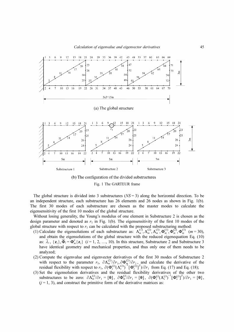
The first example presented here, GARTEUR AG-11 (as shown in Fig. 1(a)), serves to illustrate

the procedures of the calculation of eigensensitivity with the proposed substructuring method. The

frame is modeled by 78 Euler-Bernoulli beam elements and 74 nodes, as shown in Fig. 1(a). Each

node has 3 DOFs, and there are 216 DOFs in total. The Young’s modulus of each element is 75

GPa and the mass density is 2.80 × 103 kg/m3. The moment of inertia of all members is 0.0756 m4.

The cross-section areas of the vertical, horizontal and diagonal bars are 0.006 m2, 0.004 m2 and

0.003 m2, respectively.

Ψ11 0 Ψ13

0 1 0

Ψ31 0 Ψ33

vi1

vik

vi3⎩ ⎭⎪ ⎪⎨ ⎬⎪ ⎪⎧ ⎫ Yi1

0

Yi3⎩ ⎭⎪ ⎪⎨ ⎬⎪ ⎪⎧ ⎫

=

zi{ }

zi{ }T zi{ } 1=

∂ zi{ }T

∂r--------------- zi{ } zi{ }T

∂ zi{ }∂r

-------------+ 0=

vi{ }T ci zi{ }T+( ) zi{ } zi{ }T vi{ } ci zi{ }+( )+ 0=

ci1

2--- vi{ }T zi{ } zi{ }T vi{ }+( )–=

zi{ }

∂zi

∂r-------

⎩ ⎭⎨ ⎬⎧ ⎫

vi{ } 1

2--- vi{ }T zi{ } zi{ }T vi{ }+( ) zi{ }–=

Φm

p ∂Φm

p/∂r

∂zi/∂r{ }


The global structure is divided into 3 substructures (NS = 3) along the horizontal direction. To be

an independent structure, each substructure has 26 elements and 26 nodes as shown in Fig. 1(b).

The first 30 modes of each substructure are chosen as the master modes to calculate the

eigensensitivity of the first 10 modes of the global structure.

Without losing generality, the Young’s modulus of one element in Substructure 2 is chosen as the

design parameter and denoted as r1 in Fig. 1(b). The eigensensitivity of the first 10 modes of the

global structure with respect to r1 can be calculated with the proposed substructuring method:

(1) Calculate the eigensolutions of each substructure as: (m = 30),

and obtain the eigensolutions of the global structure with the reduced eigenequation Eq. (10)

as: , (i = 1, 2, …, 10). In this structure, Substructure 2 and Substructure 3

have identical geometry and mechanical properties, and thus only one of them needs to be

analyzed;

(2) Compute the eigenvalue and eigenvector derivatives of the first 30 modes of Substructure 2

with respect to the parameter r1, , and calculate the derivative of the

residual flexibility with respect to r1, from Eq. (17) and Eq. (18);

(3) Set the eigensolution derivatives and the residual flexibility derivatives of the other two

substructures to be zero: , , ,

(j = 1, 3), and construct the primitive form of the derivative matrices as:

Λm

1( )Λm

2( )Λm

3( )Φm

1( )Φm

2( )Φm

3( ), , , , ,

λi zi{ } Φi Φm

pzi{ }=,

∂Λm2( )

/∂r1 ∂Φm2( )

/∂r1,∂ Φs

2( )Λs

2( )( )1–

Φs2( )[ ]T( )/∂r1

∂Λmj( )/∂r1 0[ ]= ∂Φm

j( )/∂r1 0[ ]= ∂ Φs

j( )Λs

j( )( )1–

Φsj( )[ ]T( )/∂r1 0[ ]=

Fig. 1 The GARTEUR frame


,

(4) Obtain the first-order eigenvalue derivatives of the global structure (i = 1, 2,…10)

with Eq. (16).

(5) Calculate the first-order derivatives of with respect to the parameter r1 from

Eq. (29).

(6) Form the eigenvector derivatives of the global structure with respect to the parameter r1

according to Eq. (20) and eliminate the identical values of at the tearing interfaces.

To verify the accuracy of the proposed substructuring method in calculation of the

eigensensitivity, the traditional Nelson’s method is directly employed to calculate the

eigensensitivity of the global structure without dividing the global structure into individual

substructures. The results from the proposed substructuring method and the global method are

compared and shown in Table 1. The relative errors of the eigenvalue derivatives are less than 2%,

which is sufficient for most of practical engineering applications.

Following the concept of modal assurance criterion (MAC) (Friswell and Mottershead 1995), the

similarity of the eigenvector derivatives between the global method and the proposed substructuring

method is denoted as Correlation of Eigenvector Derivatives (COED), and given by

(30)

where represents the eigenvector derivative obtained by the global method, and

represents the eigenvector derivative by the proposed substructuring method. In this

example, the COED values are above 0.995 for all modes as listed in Table 1, which indicates good

accuracy in calculation of the eigenvector derivatives with the present method.

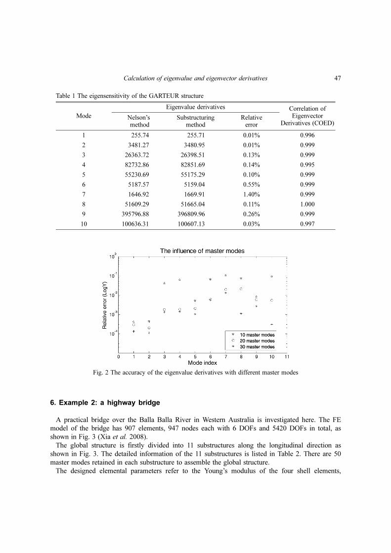
The master modes retained in the substructures affect the accuracy of the eigensensitivity

calculated. Here 10 master modes and 20 master modes in each substructure are also employed to

calculate the eigensensitivity. The relative errors of the eigenvalue derivatives are compared with the

case of 30 master modes and illustrated in Fig. 2. It can be found that, more master modes can

improve the accuracy of the eigensolution derivatives, as expected. The computational efficiency of

the proposed method will be investigated in the following example with relatively large system

matrices.

∂ Λm

p[ ]∂r1

--------------

0

∂Λm

2( )

∂r1------------

0

=∂ Φm

p[ ]∂r1

---------------

0

∂Φm

2( )

∂r1------------

0

=

∂ Φs

pΛs

p( )1–

Φs

p[ ]T

( )[ ]∂r1

-----------------------------------------------

0

∂ Φs

2( )Λs

2( )( )1–

Φs

2( )[ ]T

( )∂r1

----------------------------------------------------

0

=

∂λi/∂r1

zi{ } ∂zi/∂r1{ }

∂Φi/∂r

COED∂φi

∂r1-------

⎩ ⎭⎨ ⎬⎧ ⎫ ∂φ̃ i

∂r1--------

⎩ ⎭⎨ ⎬⎧ ⎫,

⎝ ⎠⎜ ⎟⎛ ⎞

∂φi

∂r1-------

⎩ ⎭⎨ ⎬⎧ ⎫

T

∂φ̃ i

∂r1--------

⎩ ⎭⎨ ⎬⎧ ⎫⋅

2

∂φi

∂r1-------

⎩ ⎭⎨ ⎬⎧ ⎫

T

∂φi

∂r1-------

⎩ ⎭⎨ ⎬⎧ ⎫⋅

⎝ ⎠⎜ ⎟⎛ ⎞ ∂φ̃ i

∂r1--------

⎩ ⎭⎨ ⎬⎧ ⎫

T

∂φ̃ i

∂r1--------

⎩ ⎭⎨ ⎬⎧ ⎫⋅

⎝ ⎠⎜ ⎟⎛ ⎞

--------------------------------------------------------------------------------=

∂φ̃ i/∂r1{ }∂φi/∂r1{ }


6. Example 2: a highway bridge

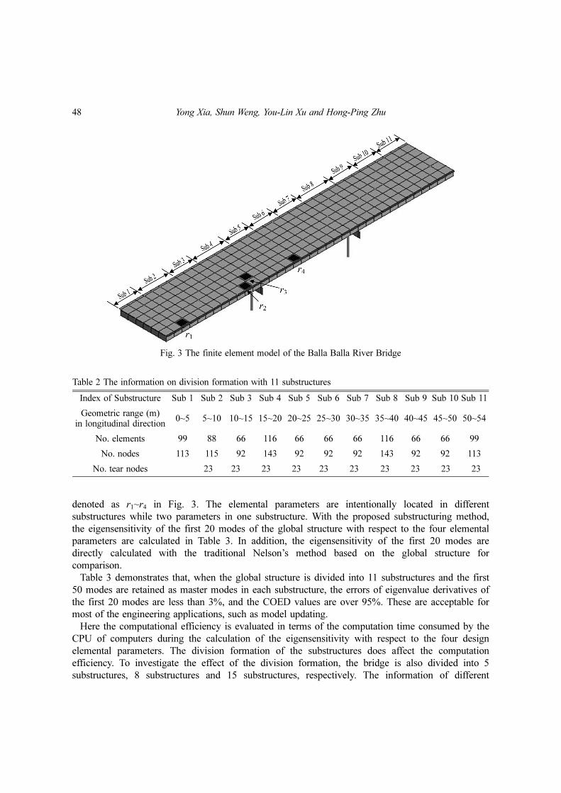
A practical bridge over the Balla Balla River in Western Australia is investigated here. The FE

model of the bridge has 907 elements, 947 nodes each with 6 DOFs and 5420 DOFs in total, as

shown in Fig. 3 (Xia et al. 2008).

The global structure is firstly divided into 11 substructures along the longitudinal direction as

shown in Fig. 3. The detailed information of the 11 substructures is listed in Table 2. There are 50

master modes retained in each substructure to assemble the global structure.

The designed elemental parameters refer to the Young’s modulus of the four shell elements,

Table 1 The eigensensitivity of the GARTEUR structure

Mode

Eigenvalue derivatives Correlation ofEigenvector

Derivatives (COED)Nelson’s method

Substructuringmethod

Relativeerror

1 255.74 255.71 0.01% 0.996

2 3481.27 3480.95 0.01% 0.999

3 26363.72 26398.51 0.13% 0.999

4 82732.86 82851.69 0.14% 0.995

5 55230.69 55175.29 0.10% 0.999

6 5187.57 5159.04 0.55% 0.999

7 1646.92 1669.91 1.40% 0.999

8 51609.29 51665.04 0.11% 1.000

9 395796.88 396809.96 0.26% 0.999

10 100636.31 100607.13 0.03% 0.997

Fig. 2 The accuracy of the eigenvalue derivatives with different master modes


denoted as r1~r4 in Fig. 3. The elemental parameters are intentionally located in different

substructures while two parameters in one substructure. With the proposed substructuring method,

the eigensensitivity of the first 20 modes of the global structure with respect to the four elemental

parameters are calculated in Table 3. In addition, the eigensensitivity of the first 20 modes are

directly calculated with the traditional Nelson’s method based on the global structure for

comparison.

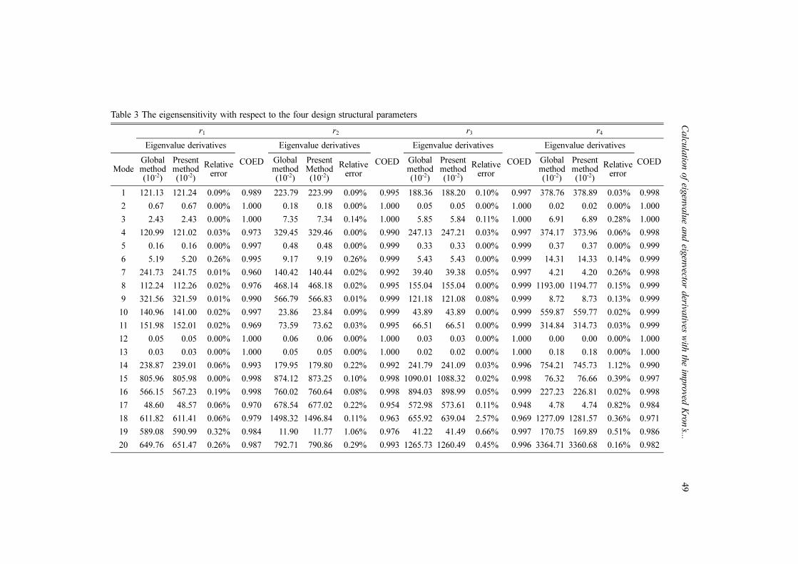
Table 3 demonstrates that, when the global structure is divided into 11 substructures and the first

50 modes are retained as master modes in each substructure, the errors of eigenvalue derivatives of

the first 20 modes are less than 3%, and the COED values are over 95%. These are acceptable for

most of the engineering applications, such as model updating.

Here the computational efficiency is evaluated in terms of the computation time consumed by the

CPU of computers during the calculation of the eigensensitivity with respect to the four design

elemental parameters. The division formation of the substructures does affect the computation

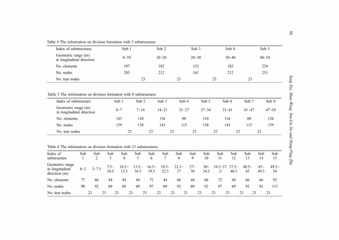
efficiency. To investigate the effect of the division formation, the bridge is also divided into 5

substructures, 8 substructures and 15 substructures, respectively. The information of different

Fig. 3 The finite element model of the Balla Balla River Bridge

Table 2 The information on division formation with 11 substructures

Index of Substructure Sub 1 Sub 2 Sub 3 Sub 4 Sub 5 Sub 6 Sub 7 Sub 8 Sub 9 Sub 10 Sub 11

Geometric range (m)in longitudinal direction

0~5 5~10 10~15 15~20 20~25 25~30 30~35 35~40 40~45 45~50 50~54

No. elements 99 88 66 116 66 66 66 116 66 66 99

No. nodes 113 115 92 143 92 92 92 143 92 92 113

No. tear nodes 23 23 23 23 23 23 23 23 23 23

Calcu

latio

n o

f eigen

valu

e and eig

envecto

r deriva

tives with

the im

pro

ved K

ron’s...

49

Table 3 The eigensensitivity with respect to the four design structural parameters

r1 r2 r3 r4

Eigenvalue derivatives

COED


COED


COED


COEDMode

Global method(10-2)

Presentmethod(10-2)

Relative error

Global method(10-2)

PresentMethod(10-2)

Relative error

Global method(10-2)

Presentmethod(10-2)

Relative error

Global method(10-2)

Presentmethod(10-2)

Relative error

1 121.13 121.24 0.09% 0.989 223.79 223.99 0.09% 0.995 188.36 188.20 0.10% 0.997 378.76 378.89 0.03% 0.998

2 0.67 0.67 0.00% 1.000 0.18 0.18 0.00% 1.000 0.05 0.05 0.00% 1.000 0.02 0.02 0.00% 1.000

3 2.43 2.43 0.00% 1.000 7.35 7.34 0.14% 1.000 5.85 5.84 0.11% 1.000 6.91 6.89 0.28% 1.000

4 120.99 121.02 0.03% 0.973 329.45 329.46 0.00% 0.990 247.13 247.21 0.03% 0.997 374.17 373.96 0.06% 0.998

5 0.16 0.16 0.00% 0.997 0.48 0.48 0.00% 0.999 0.33 0.33 0.00% 0.999 0.37 0.37 0.00% 0.999

6 5.19 5.20 0.26% 0.995 9.17 9.19 0.26% 0.999 5.43 5.43 0.00% 0.999 14.31 14.33 0.14% 0.999

7 241.73 241.75 0.01% 0.960 140.42 140.44 0.02% 0.992 39.40 39.38 0.05% 0.997 4.21 4.20 0.26% 0.998

8 112.24 112.26 0.02% 0.976 468.14 468.18 0.02% 0.995 155.04 155.04 0.00% 0.999 1193.00 1194.77 0.15% 0.999

9 321.56 321.59 0.01% 0.990 566.79 566.83 0.01% 0.999 121.18 121.08 0.08% 0.999 8.72 8.73 0.13% 0.999

10 140.96 141.00 0.02% 0.997 23.86 23.84 0.09% 0.999 43.89 43.89 0.00% 0.999 559.87 559.77 0.02% 0.999

11 151.98 152.01 0.02% 0.969 73.59 73.62 0.03% 0.995 66.51 66.51 0.00% 0.999 314.84 314.73 0.03% 0.999

12 0.05 0.05 0.00% 1.000 0.06 0.06 0.00% 1.000 0.03 0.03 0.00% 1.000 0.00 0.00 0.00% 1.000

13 0.03 0.03 0.00% 1.000 0.05 0.05 0.00% 1.000 0.02 0.02 0.00% 1.000 0.18 0.18 0.00% 1.000

14 238.87 239.01 0.06% 0.993 179.95 179.80 0.22% 0.992 241.79 241.09 0.03% 0.996 754.21 745.73 1.12% 0.990

15 805.96 805.98 0.00% 0.998 874.12 873.25 0.10% 0.998 1090.01 1088.32 0.02% 0.998 76.32 76.66 0.39% 0.997

16 566.15 567.23 0.19% 0.998 760.02 760.64 0.08% 0.998 894.03 898.99 0.05% 0.999 227.23 226.81 0.02% 0.998

17 48.60 48.57 0.06% 0.970 678.54 677.02 0.22% 0.954 572.98 573.61 0.11% 0.948 4.78 4.74 0.82% 0.984

18 611.82 611.41 0.06% 0.979 1498.32 1496.84 0.11% 0.963 655.92 639.04 2.57% 0.969 1277.09 1281.57 0.36% 0.971

19 589.08 590.99 0.32% 0.984 11.90 11.77 1.06% 0.976 41.22 41.49 0.66% 0.997 170.75 169.89 0.51% 0.986

20 649.76 651.47 0.26% 0.987 792.71 790.86 0.29% 0.993 1265.73 1260.49 0.45% 0.996 3364.71 3360.68 0.16% 0.982

50

Yong X

ia, S

hun W

eng, Yo

u-L

in X

u a

nd H

ong-P

ing Z

hu


Index of substructures Sub 1 Sub 2 Sub 3 Sub 4 Sub 5


0~10 10~20 20~30 30~40 40~54

No. elements 187 182 132 182 224

No. nodes 205 212 161 212 251

No. tear nodes 23 23 23 23


Index of substructure Sub 1 Sub 2 Sub 3 Sub 4 Sub 5 Sub 6 Sub 7 Sub 8


0~7 7~14 14~21 21~27 27~34 35~41 41~47 47~54

No. elements 143 110 116 88 110 116 88 136

No. nodes 159 138 143 115 138 143 115 159

No. tear nodes 23 23 23 23 23 23 23


Index of substructure

Sub1

Sub2

Sub3

Sub4

Sub5

Sub6

Sub7

Sub8

Sub9

Sub10

Sub11

Sub12

Sub13

Sub14

Sub15

Geometric rangein longitudinal direction (m)

0~3 3~7.57.5~10.5

10.5~13.5

13.5~16.5

16.5~19.5

19.5~22.5

22.5~27

27~30

30~34.5

34.5~37.5

37.5~40.5

40.5~45

45~49.5

49.5~54

No. elements 77 66 44 44 44 72 44 66 44 66 72 44 66 66 92

No. nodes 90 92 69 69 69 97 69 92 69 92 97 69 92 92 113

No. tear nodes 23 23 23 23 23 23 23 23 23 23 23 23 23 23


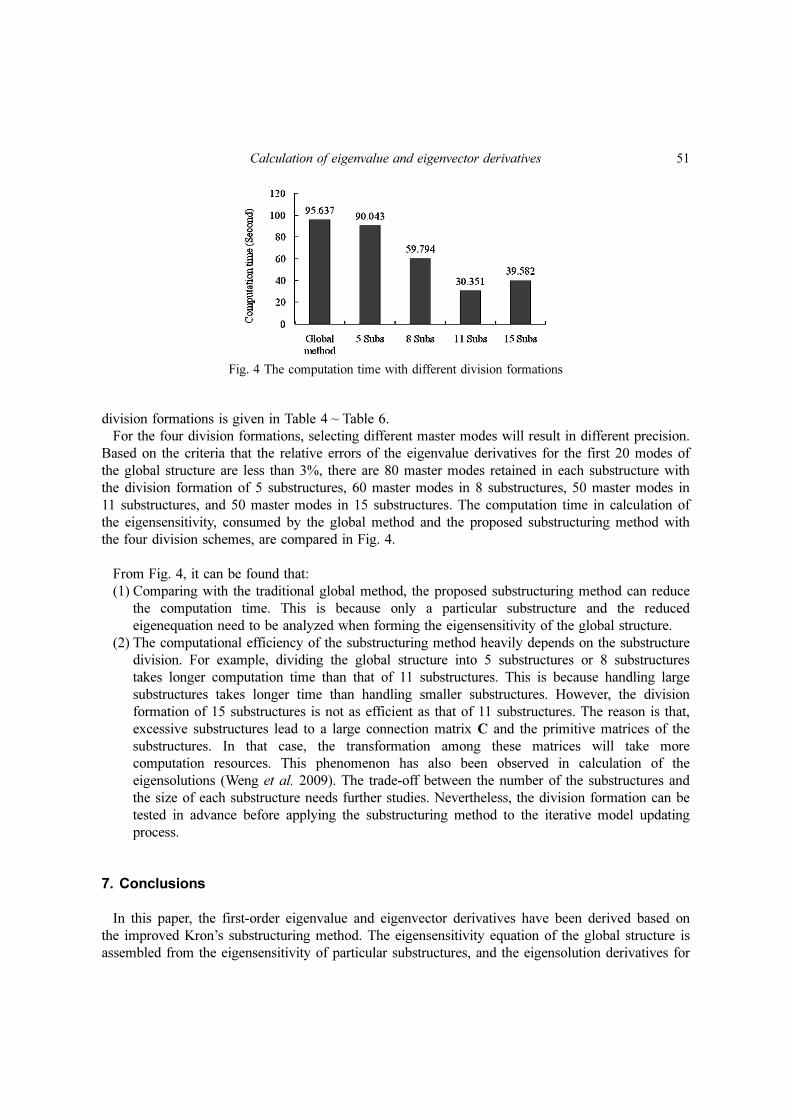
division formations is given in Table 4 ~ Table 6.

For the four division formations, selecting different master modes will result in different precision.

Based on the criteria that the relative errors of the eigenvalue derivatives for the first 20 modes of

the global structure are less than 3%, there are 80 master modes retained in each substructure with

the division formation of 5 substructures, 60 master modes in 8 substructures, 50 master modes in

11 substructures, and 50 master modes in 15 substructures. The computation time in calculation of

the eigensensitivity, consumed by the global method and the proposed substructuring method with

the four division schemes, are compared in Fig. 4.

From Fig. 4, it can be found that:

(1) Comparing with the traditional global method, the proposed substructuring method can reduce

the computation time. This is because only a particular substructure and the reduced

eigenequation need to be analyzed when forming the eigensensitivity of the global structure.

(2) The computational efficiency of the substructuring method heavily depends on the substructure

division. For example, dividing the global structure into 5 substructures or 8 substructures

takes longer computation time than that of 11 substructures. This is because handling large

substructures takes longer time than handling smaller substructures. However, the division

formation of 15 substructures is not as efficient as that of 11 substructures. The reason is that,

excessive substructures lead to a large connection matrix C and the primitive matrices of the

substructures. In that case, the transformation among these matrices will take more

computation resources. This phenomenon has also been observed in calculation of the

eigensolutions (Weng et al. 2009). The trade-off between the number of the substructures and

the size of each substructure needs further studies. Nevertheless, the division formation can be

tested in advance before applying the substructuring method to the iterative model updating

process.

7. Conclusions

In this paper, the first-order eigenvalue and eigenvector derivatives have been derived based on

the improved Kron’s substructuring method. The eigensensitivity equation of the global structure is

assembled from the eigensensitivity of particular substructures, and the eigensolution derivatives for

Fig. 4 The computation time with different division formations


the reduced eigenequation are then calculated emulating the Nelson’s method. Two numerical

examples demonstrate that the proposed method can achieve a good accuracy when the proper

master modes are retained.

The division formation of the global structure should be considered with caution. Too few

substructures, which result in large-size substructures, might reduce the efficiency of the

substructuring method. However, excessive substructures may introduce a large transformation

matrix, and accordingly cause the assembly of the substructures to the global structure time-

consuming. One should trade off the number of the substructures and the size of each substructure.

Retaining more master modes in the substructures can achieve a better accuracy while cost more

computation resource. The error estimation is required for the selection of the master modes in the

substructures, which will be studied in the future. Moreover, further research will focus on how to

improve the accuracy of the proposed substructuring method and implement it to the model

updating process.

Acknowledgements

The work described in this paper is jointly supported by a grant from the Research Grants Council

of the Hong Kong Special Administrative Region, China (Project No. PolyU 5321/08E) and a grant

from Natural Science Foundation, China (Project No. 50830203).

References

Bakir, P.G., Reynders, E. and Roeck, De G. (2007), “Sensitivity-based finite element model updating usingconstrained optimization with a trust region algorithm”, J. Sound Vib., 305(1-2), 211-225.

Brownjohn, J.M.W., Xia, P.Q., Hao, H. and Xia, Y. (2001), “Civil structure condition assessment by FE modelupdating: methodology and case studies”, Finite Elem. Anal. Des., 37(10), 761-775.

Choi, D., Kim, H. and Cho, M. (2008), “Iterative method for dynamic condensation combined withsubstructuring scheme”, J. Sound Vib., 317(1-2), 199-218.

Craig, Jr. R.R. and Bampton, M.M.C. (1968), “Coupling of substructures for dynamic analysis”, AIAA J., 6(7),1313-1319.

Craig, Jr. R.R. (2000), “Coupling of substructures for dynamic analysis: an overview”, Proceedings of the 41stAIAA/ASCE/AHS/ASC Structures, Structural Dynamics, and Materials Conference and Exhibit, AIAA-2000-1573, Atlanta, GA, April.

Felippa, C.A., Park, K.C. and Justino Filho, M.R. (1998), “The construction of free-free flexibility matrices asgeneralized stiffness inverses”, Comput. Struct., 68(4), 411-418.

Fox, R.L. and Kapoor, M.P. (1968), “Rate of change of eigenvalues and eigenvectors”, AIAA J., 6(12), 2426-2429.

Friswell, M.I. and Mottershead, J.E. (1995), Finite Element Model Updating in Structural Dynamics, KluwerAcademic Publishers.

Fulton, R.E. (1991), “Structural dynamics method for parallel supercomputers”, Report for MacNeal SchwendlerCorp.

Hurty, W.C. (1965), “Dynamic analysis of structural systems using component modes”, AIAA J., 3(4), 678-685.Kron, G. (1963), Diakoptics, Macdonald and Co., London.Lin, R.M. and Lim, M.K. (1995), “Structural sensitivity analysis via reduced-order analytical model”, Comput.

Meth. Appl. Mech. Eng., 121(1-4), 345-359.Lin, R.M. and Lim, M.K. (1996a), “Eigenvector derivatives of structures with rigid body modes”, AIAA J.,


34(5), 1083-1085.Lin, R.M., Wang, Z. and Lim, M.K. (1996b), “A practical algorithm for efficient computation of eigenvector

sensitivities”, Comput. Meth. Appl. Mech. Eng., 130, 355-367.MacNeal, R.H. (1971), “A hybrid method of component mode synthesis”, Comput. Struct., 1(4), 581-601.Nelson, R.B. (1976), “Simplified calculation of eigenvector derivatives”, AIAA J., 14(9), 1201-1205.Qiu, J.B., Ying, Z.G. and Williams, F.W. (1997), “Exact modal synthesis techniques using residual constraint

modes”, Int. J. Numer. Meth. Eng., 2475-2492.Rubin, S. (1975), “Improved component-mode representation for structural dynamic analysis”, AIAA J., 13(8),

995-1005.Sehmi, N.S. (1986), “The Lanczos algorithm applied to Kron’s method”, Int. J. Numer. Meth. Eng., 23, 1857-

1872.Sehmi, N.S. (1989), Large Order Structural Eigenanalysis Techniques Algorithms for Finite Element Systems,

Ellis Horwood Limited, Chichester, England.Simpson, A. (1973), “Eigenvalue and vector sensitivities in Kron's method”, J. Sound Vib., 31(1), 73-87.Simpson, A. and Tabarrok, B. (1968), “On Kron’s eigenvalue procedure and related methods of frequency

analysis”, Quarterly Journal of Mechanics and Applied Mathematics, 21, 1039-1048.Song, D.T., Han, W.Z., Chen, S.H. and Qiu, Z.P. (1996), “Simplified calculation of eigenvector derivatives with

repeated eigenvalues”, AIAA J., 34(4), 859-861.Turner, G.L. (1983), Finite Element Modeling and Dynamic Substructuring for Prediction of Diesel Engine

Vibration, Ph.D thesis, Loughborough University of Technology.Weng, S. and Xia, Y. (2007), “Substructure method in eigensolutions and model updating for large scale

structures,” Proceedings of the 2nd International Conference on Structural Condition Assessment, Monitoringand Improvement, Changsha, China.

Weng, S., Xia, Y., Xu, Y.L., Zhou, X.Q. and Zhu, H.P. (2009), “Improved substructuring method foreigensolutions of large-scale structures”, J. Sound Vib., 323(3-5), 718-736.

Wu, B.S., Xu, Z.H. and Li, Z.G. (2007), “Improved Nelson’s method for computing eigenvector derivatives withdistinct and repeated eigenvalues”, AIAA J., 45(4), 950-952.

Xia, Y., Hao, H., Deeks, A.J. and Zhu, X.Q. (2008), “Condition assessment of shear connectors in slab-girderbridges via vibration measurements”, J. Bridge Eng., 13(1), 43-54.

Xia,Y. and Lin, R.M. (2004), “A new iterative order reduction (IOR) method for eigensolutions of largestructures”, Int. J. Numer. Meth. Eng., 59, 153-172.

Yun, C.B. and Lee, H.J. (1997), “Substructural identification for damage estimation of structures”, Struct. Saf.,19(1), 121-140.


Appendix: The residual flexibility and the derivatives for the free-free substructures

Without losing generality, here the residual flexibility and the derivative matrix are derived for an arbitrarystructure with the stiffness and mass matrices of K and M, respectively.

The free-free structure has two kinds of eigenmodes: the nr rigid body modes R and the nd deformationalmodes Φd. The orthogonality of the rigid body modes satisfies

(A. 1)

Due to the fact that , an orthogonal projector associated with R can be constructed as

(A. 2)

The orthogonality properties yield the spectral decompositions as

, (A. 3)

Since , including the rigid body modes into the free-free stiffness matrix K similarly gives

, (A. 4)

The eigenvector of are identical to those of K, but including the rigid body modes and setting theeigenvalues of rigid body modes to be unity.

The complete eigenmodes are divided into nm master modes Φm and ns slave modes Φs according to themain sections of this paper. The master modes Φm are composed by the nr rigid body master modes R and the(nm− nr) normal master modes Φm-r. The deformational modes include the master modes Φm-r and the slavemodes Φs. Eq. (A.4) is equivalent to

(A. 5)

The residual flexibility for the free-free structure is

(A. 6)

Accordingly, for the fixed structure without zero-frequency modes, the rigid-body modes are vanished, andthe residual flexibility is simplified as usual form

(A. 7)

Considering the mass matrix, the orthogonal condition satisfies

(A. 8)

Decomposing the mass matrix as , and denoting

(A. 9)

RTR I=

I RRT

–( )RRT

0=

P I RRT

–=

P ΦdΦd

T

i 1=

Nd

∑= P RRT

+ ΦdΦd

T

i 1=

Nd

∑ RRT

+=

K λiΦdΦd

T

i 1=

Nd

∑=

K RRT

+ λiΦdΦd

T

i 1=

Nd

∑ RRT

+= K RRT

+( )1– 1

λi

----ΦdΦd

T

i 1=

Nd

∑ RRT

+=

K RRT

+

M M1/2M

1/2=


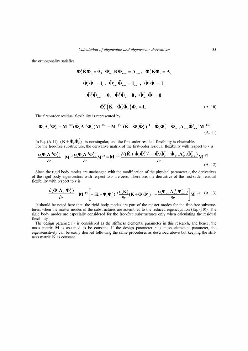
the orthogonality satisfies

(A. 10)

The first-order residual flexibility is represented by

(A. 11)

In Eq. (A.11), is nonsingular, and the first-order residual flexibility is obtainable.For the free-free substructure, the derivative matrix of the first-order residual flexibility with respect to r is

(A. 12)

Since the rigid body modes are unchanged with the modification of the physical parameter r, the derivativesof the rigid body eigenvectors with respect to r are zero. Therefore, the derivative of the first-order residualflexibility with respect to r is

(A. 13)

It should be noted here that, the rigid body modes are part of the master modes for the free-free substruc-tures, when the master modes of the substructures are assembled to the reduced eigenequation (Eq. (10)). Therigid body modes are especially considered for the free-free substructures only when calculating the residualflexibility.

The design parameter r is considered as the stiffness elemental parameter in this research, and hence, themass matrix M is assumed to be constant. If the design parameter r is mass elemental parameter, theeigensensitivity can be easily derived following the same procedures as described above but keeping the stiff-ness matrix K as constant.

K̃ Φ̃rΦ̃r

T+( )

calculation of eigenvalue and eigenvector derivatives with...

Documents