geographic concentration and vertical disintegration ... · geographic concentration and vertical...

Title Geographic concentration and vertical disintegration: Evidencefrom China

Author(s) Li, B; Lu, Y

Citation Journal Of Urban Economics, 2009, v. 65 n. 3, p. 294-304

Issued Date 2009

URL http://hdl.handle.net/10722/60229

Rights Creative Commons: Attribution 3.0 Hong Kong License

Geographic Concentration and Vertical Disintegration:

Evidence from China♣

Current version: December, 2008

Forthcoming at Journal of Urban Economics

Ben Li

Department of Economics University of Colorado, Boulder

USA Email: [email protected]

Yi Lu* Faculty of Business and Economics

University of Hong Kong Hong Kong

Email: [email protected]

Abstract Existing theoretical literature predicts that geographic concentration encourages vertical disintegration of firms. Nevertheless, empirical evidence of this prediction is limited, especially in developing countries. Using data on manufacturing firms from China, this paper documents a positive correlation between geographic concentration and vertical disintegration. Additionally, this paper uses the instrumental variable approach to address the issue of endogeneity and finds that geographic concentration has a positive causal effect on vertical disintegration. Keywords: Geographic concentration, vertical disintegration, outsourcing, China. JEL Code: R30, L23, D21.

♣ We are grateful for the helpful comments by Julan Du, Thomas Holmes, Wolfgang Keller, Zhigang Tao, Donald Waldman, as well as seminar participants at the 2007 IOMS Summer Workshop. We particularly thank the editor and two anonymous referees for their comments. Any remaining errors are ours. * Corresponding author: Y. Lu. Address: Faculty of Business and Economics, University of Hong Kong, Pokfulam Road, HK. Email: [email protected].

Geographic Concentration and Vertical Disintegration: Evidence from China

1. Introduction

Existing theoretical literature suggests that geographic concentration of industries has important

effects on the organization of individual firms. Marshall (1920) points out that geographic

concentration facilitates input sharing among firms,1 and Stigler (1951) argues that input sharing

can make firms more vertically disintegrated. Recent work further explores the mechanisms

through which geographic concentration promotes vertical disintegration, such as lowering cost

(Goldstein and Gronberg, 1984) and reducing opportunism (Helsley and Strange, 2007).

Empirical evidence regarding the relationship between geographic concentration and

vertical disintegration has not accumulated significantly. Although a number of case studies

show a connection between specialized suppliers and vertical disintegration,2 it remains unclear

whether such a connection can be generalized to other industries.3 Holmes (1999) carries out the

first rigorous empirical test using data from the 1987 U.S. Census of Manufacturers, and finds a

positive correlation between geographic concentration and vertical disintegration.

This paper uses Chinese manufacturing data to further investigate the impacts of geographic

concentration on vertical disintegration. The economic conditions in China, the largest

developing economy in the world, are substantially different from those in the U.S. Several

factors prompt us to investigate the relationship between geographic concentration and vertical

disintegration in China. First, overall industrial concentration is considerably lower in China than

in the U.S. According to the EG Index (Ellison and Glaeser, 1997), 80 percent of four-digit

1 Input sharing is one type of Marshallian externality. Marshallian externalities also include knowledge spillover and labor market pooling. See Strange (2005) for details. 2 See, for example, Allen (1929) with regard to the gun industry in nineteenth-century Birmingham, Hall (1959) and Lichtenberg (1960) concerning a number of industries that concentrate in New York, and Scott and Kwok (1989) on the printed circuit industry in Southern California. More evidence can be found in Scott (1988, 2000). 3 One important reason is that firm-level data were seldom available in the past (Yang and Ng, 1993; Zhang, 2004).

1

industries in China are classified as not very concentrated, whereas only 10 percent in the U.S.

can be considered as belonging to the same group (Lu and Tao, 2008). Compared to the U.S.

economy, the Chinese economy is much less integrated as a whole (Young, 2000; Poncet, 2003),

a factor that may obstruct the process of geographic concentration.

Second, in China, the agricultural sector employs about half the national labor force, and

town and village enterprises account for nearly a third of firms in the manufacturing sector (Au

and Henderson, 2002). In contrast, more than 75 percent of the U.S. populace lives in cities

(Rosenthal and Strange, 2006). Such structural differences in the labor force and in the

manufacturing sector may produce different patterns of industrial concentration and vertical

disintegration (Picard and Zeng, 2005).

Third, compared to the U.S., China is an unskilled-labor abundant economy where simple

processing and assembly activities predominate, thus placing it at the lower end of the world

value chain. Different production activities may cause differences in the organization of

production, and we accordingly seek to determine whether manufacturing of low added-value

products has the same relationship between geographic concentration and vertical disintegration.

Our study first replicates the analysis in Holmes (1999) using Chinese data, and discovers a

similar relationship between geographic concentration and vertical disintegration. Within the

same region and four-digit industry, the ratio of purchased intermediate inputs over output rises

with own-industry neighboring employment, suggesting that the positive correlation between

geographic concentration and vertical disintegration initially found by Holmes in the U.S. also

holds in China. This positive correlation is robust to different specifications, such as including

nonlinear terms, using more disintegrated (firm/region-level) data,4 and controlling for

firm/region-level characteristics. Our firm/region-level investigation also provides suggestive 4 Details on the data set will be discussed in Section 3.

2

evidence of Stigler’s (1951) hypothesis; namely, the extent of vertical integration increases for

young and very old firms, and decreases for mature firms.

Although Holmes (1999) provides an important contribution, it is still difficult to pinpoint

the causality between geographic concentration and vertical disintegration due to endogeneity.

For example, some missing variables causing both vertical disintegration and geographic

concentration can induce a spurious positive correlation between the two. It is also possible that

the presence of local suppliers encourages localization and thus reverses the causality.

As a second contribution, we investigate whether geographic concentration has a causal

effect on the degree of vertical disintegration using instrumental-variable estimation. Specifically,

we use the cross-region population of China in 1920 to instrument China’s geographic

concentration of industries in 2002.5 The validity of our instrumental variable is based on two

premises: (1) the demand of a larger population attracts more manufacturers in each industry,6

and (2) the distribution of population persists over time (Davis and Weinstein, 2002). In other

words, the geographic concentration of industries in 2002 varies with the distribution of

population as it stood more than 80 years ago, which should have no direct effect on the current

degree of vertical disintegration of firms. Figure 1 summarizes our instrumental variable

estimation strategy.

[Figure 1 about here]

The two-stage-least-squares (2SLS) estimates substantiate our early findings, showing that

geographic concentration leads firms to be more vertically disintegrated. Moreover, this effect is

stronger than what is captured by the ordinary-least-squares (OLS) estimates.

The rest of the paper is organized as follows. Section 2 presents a brief review of the related

5 As for the practice of using historical data as instrumental variables, see, for instance, Acemoglu et al. (2001, 2002). 6 See Krugman (1980) for a theoretical model, and Davis and Weinstein (2003) and Hanson (2005) for empirical supports.

3

literature. Section 3 describes the data and procedures used in constructing the data set. Sections

4 and 5 report and discuss the OLS and 2SLS results, respectively, including robustness checks.

Section 6 summarizes our findings and suggests directions for future research.

2. Literature

A fundamental question in economics concerns the factors that determine the degree of vertical

integration (or disintegration) of firms. This question can be traced back to Adam Smith (1776,

Chapter 1), who discusses the division of labor within firm boundaries and the relationship

between the division of labor and productivity. The idea is extended to specialization among

firms (Stigler, 1951; Young, 1928), and is tested by Murakami et al. (1996). Stigler (1951)

proposes another theory on vertical specialization through the lens of industry lifecycle, and his

main insights are empirically confirmed by Tucker and Wilder (1977) and Levy (1984).

Two distinct approaches emerge in the study of vertical integration. One is the

industrial-organization approach, which mainly attributes vertical integration to imperfect

competition, technological externalities, and asymmetric information.7 The other approach

examines vertical integration in the context of transaction cost theory (e.g., Coase, 1937;

Williamson, 1975, 1985) and property rights theory (e.g., Grossman and Hart, 1986; Hart and

Moore, 1990; Hart, 1995). These authors consider specific investment and hold-up issues, which

interact to determine the degree of vertical integration.8 Recently, interest in the determinants of

vertical integration has resurfaced.9 In particular, the recent rapid growth of international trade

7 See Perry (1989) for a review of the literature. 8 There are also empirical studies using this approach. For instance, Baker and Hubbard (2004), Feenstra and Hanson (2005), Hortaçsu and Syverson (2007), Joskow (1987), Lieberman (1991), Masten (1984), and Monteverde and Teece (1982). 9 To this end, there have been theoretical (e.g., Chen, 2005; Chen and Riordan, 2007) as well as empirical (e.g., Acemoglu et al. 2005, 2007a, 2007b) advancements.

4

has made firms more vertically disintegrated across borders,10 and has inspired a number of

theoretical papers, for instance, Antràs (2003), Antràs and Helpman (2004, 2006), Antràs et al.

(2006), Grossman and Helpman (2002, 2004, 2005), McLaren (1999), and Puga and Trefler

(2002).11

Our paper extends the discussion of vertical disintegration to include a consideration of the

effects of geographic concentration on individual firms. There are two primary underlying

reasons for the association between geographic concentration and vertical disintegration. First,

Goldstein and Gronberg (1984) indicate that geographic concentration encourages vertical

disintegration by lowering delivered prices for inputs based on proximity to suppliers.12 Second,

geographic concentration reduces opportunism, and thus substitutes for vertical integration

(Helsley and Strange, 2007).

3. Data and Statistics

Our primary data source is the National Statistical Bureau Enterprise Dataset 2002 (NSBED

2002). The NSBED is a large-scale data set maintained by the National Statistical Bureau of

China. It contains approximately 100 variables at the firm/region level, including sales revenue,

location, four-digit industry code, founding year, and employment. The industry section of the

China Statistical Yearbook 2003 was compiled based on this data set. To maintain comparability

with Holmes (1999), we focus on the manufacturing industries in the NSBED, and follow his

procedures in constructing our data set.

As the most comprehensive micro-level data set in China mainland, the NSBED collects

10 See, for example, Feenstra (1998), Hanson et al. (2005), and Hummels, et al. (1998). 11 See Spencer (2005), Antràs (2006), and Helpman (2006) for reviews of the literature. 12 Transport costs have long been identified to comprise the main reason for the geographic concentration of industries since Thünen (1826), see Keilbach (2000, Chap.3). Krugman (1991) and Krugman and Venables (1995) address the important role of transport costs with distinct models, and it is widely accepted that transport costs penalize vertical integration (Hummels et al., 2001). As for how geographic concentration affects input sharing, see Duranton and Puga (2001) and Helsley and Strange (2002).

5

data at the firm/region level. A firm may or may not have business operations located in regions

other than its domicile.13 If a firm has no business operations outside its domicile, the company

itself constitutes a firm/region-level observation in the data set. If a firm has branches that

engage in business operations in regions other than its domicile, each branch constitutes a

firm/region-level observation in the data set. For example, Beijing Huiyuan Beverage and Food

Group Co., Ltd. has six branches, in Jizhong (Hebei Province), Youyu (Shanxi Province),

Luzhong (Shandong Province), Qiqihar (Heilongjiang Province), Chengdu (Sichuan Province),

and Yanbian (Jilin Province); the NSBED accordingly counts them as six different

firm/region-level observations belonging to six different regions, in addition to their parent

company located in Beijing.

It is noteworthy that the U.S. census data used by Holmes (1999) are collected at the plant

level, which is more disaggregated than the firm/region level. Data collected at the firm/region

level have certain advantages over those collected at the plant level for our purposes. First, as

Eckard (1979) points out, the U.S. census assigns an industry code to a plant according to the

primary output of this plant; consequently, an integrated plant remains in its initial industry, and

thus a cross-industry transaction between it and its parent is counted as outsourcing. In the

NSBED, such a transaction will not be counted as outsourcing. In addition, outsourcing decisions,

which affect the competitive strategies of firms, are more likely to be made at the firm/region

level (the regional headquarter) rather than at the plant level.

In our exercise, the set of firm/region-level observations that belong to four-digit industry

and region is denoted by , =1,...,518, and =1,...,31.

i

a ( , )i aE i a 14 The costs of intermediate

13 Regions refer to 31 province-level regions in China, including 22 provinces, 5 autonomous regions, and 4 municipalities. 14 Due to limitations in the official data-collecting practice, the economic literature that investigates the agglomeration in China typically uses province-level or more aggregated data. See, for instance, Wen (2004) and Bai et al. (2004). Additionally, we use province-level region data because the province-level in China is similar to the state-level in the U.S. Input sharing is the most

6

inputs divided by sales revenue is defined as the purchased-inputs intensity (PII) for a

firm/region-level observation , and is used to measure the degree of vertical

disintegration.

),(∈ aiEx

15 These firm/region-level statistics are then aggregated to the industry/region

level by

( , )

( , )i a

i a x xx EPII w PII

∈=∑ ,

where is the purchased-inputs intensity of , and is the share of a given ),( aiPII ),( ai xw x in

the total output of ),( ai

( , )i a

xx

xx E

outputwoutput

∈

=∑

.

Since plant-level output is unavailable in Holmes’ (1999) data set, he uses employment share

instead. Fortunately, firm/region-level employment and output are both available in the NSBED

2002, so we use both weights in this paper.

We implement this study primarily at the industry/region level, and use firm/region-level

findings only as robustness checks. There are several reasons for this strategy. First, we intend

for our findings to be comparable to those of Holmes (1999), which aggregates available

plant-level data to the industry/region level. Second, an inherent defect of PII is that it can be

easily contaminated by micro-level productivity heterogeneity. Higher productivity can increase

added value, thereby decreasing the ratio of purchased intermediate inputs over output, which is

likely to be misinterpreted as less vertical disintegration. Productivity heterogeneity arguably

cancels out at more aggregated levels—such as the industry/region level—and consequently likely determinant in our context; Rosenthal and Strange (2001) find that reliance on inputs positively affects agglomeration at the state level, but this effect hardly exists at lower levels of the geographic unit. 15 There are a number of methods to measure vertical integration (or disintegration). For example, Chapman and Ashton (1914) use the number of equipment items; Gort (1962) uses employment in each industry; Guidelines for Vertical Restraints (1985) of the U.S. Department of Justice use the Herfindahl-Hirsclman index; Acemoglu et al. (2007b) use vertical integration coefficients. PII originates from Adelman (1955), and is widely used in the literature, e.g., Laffer (1969), Tucker and Wilder (1977), Levy (1984), and Holmes (1999). For a detailed discussion of vertical-integration measurement, see Perry (1989).

7

eliminates productivity heterogeneity from the measured degree of vertical disintegration. Third,

as discussed in the next section, our instrumental-variable data are available only at the region

level.

The employment of neighboring firms is used to measure geographic concentration. We

define three types of neighboring firms. Own-industry neighboring firms for a given x is the

observations other than x located in the same four-digit industry/region; their total employment

is denoted by . Own-industry neighboring employment in each is defined to be ownxEMP ),( ai

( , )

( , )i a

own owni a x xx E

EMP w EMP∈

=∑ .

Related-industry neighboring firms for a given x are defined as those belonging to the

same two-digit industry as x but different four-digit industries. Their total employment is

denoted by . Related-industry neighboring employment is defined to be relatedxEMP

( , )

( , )i a

related relatedi a x xx E

EMP w EMP∈

=∑ .

Finally, we introduce other-industry neighboring firms for a given x , each of which is

neither x ’s own-industry neighboring observations nor x ’s related-industry neighboring

observations, while they are in the same region as x . Other-industry neighboring employment

),a is defined in i as (

( , )

( , )i a

other otheri a x xx E

EMP w EMP∈

=∑ .

Table 1 summarizes the industry/region-level data set we use in this paper. Panels A and B

report the descriptive statistics of variables weighted by employment and output, respectively.

The statistics for related- and other-industry neighboring employment are identical in these two

panels, because the firms within the same industry/region have the same set of related- and

other-industry neighboring firms. The weighted sums of employment in these observations are

8

thus equal, whichever weights are adopted. Panel C presents descriptive statistics of the

instrumental variable, as well as other related information. The data on region-level population

for China in 1920, our instrumental variable, were collected by the China Continuation

Committee, a western missionary organization.16 In the absence of a national statistical

institution in China in the 1920s, this constitutes one of the most reliable data sources.

[Table 1 about here]

4. The OLS results

The first model in Holmes (1999) is specified as

* *( , ) ( , ) ( , )= +owni a i a i aPII αEMP ε*

,

where the asterisk means that the variable is demeaned by its industry average. By demeaning

the variables, this specification controls for industry fixed effects. Weighted-least-squares (WLS)

technique is then used to estimate the model, and the weights are given according to the number

of firm/region-level observations in each , with a correction to account for the asymmetry

of size among these observations.

),( ai

17,18 In Model 2 and Model 3, and are

incorporated sequentially. Model 4 introduces squared and cubic terms for each explanatory

variable. His results are reproduced in Table 2a.

relatedxEMP other

xEMP

[Table 2a about here]

We estimate Models 1–4 using Chinese data following the same procedure, and the results

are reported in Table 2b. Model 1 demonstrates a positive correlation between PII and

own-industry neighboring employment. The estimated coefficient is 0.017 (s.e.=0.001), which

16 Specifically, the data were collected by the Special Committee on Survey and Occupation of China Continuation Committee. Note that the divisions of regions used by the China Continuation Committee differ from those under the current Chinese regime, so that the population of each region has been recalculated according to the current regional divisions. 17 See the appendix of Holmes (1999) for details on constructing this weight. 18 We re-estimate these models without weights and obtain nearly identical results. Results are available upon request.

9

means that the conditional expectation of PII increases by 0.017 percentage points if

own-industry neighboring employment increases by 1,000. In terms of standard deviation, if

own-industry neighboring employment increases by one standard deviation, PII would rise by

0.228 (0.017 times 13.4) percentage points. This is comparable to Holmes’ (1999) finding with

the U.S. census data: PII rises by 0.188 (0.04 times 4.7)19 percentage points if own-industry

neighboring employment increases by one standard deviation.

[Table 2b about here]

The rationale behind this positive correlation is straightforward. Consider two motor-vehicle

manufacturers, one locating where peers are geographically concentrated, and the other not.

Ceteris paribus, the first motor-home manufacturer, would have a higher PII because it can

locally outsource parts at lower costs (not limited to lower transport costs), whereas the other

lacks this advantage. Another interpretation of this finding is that industrial concentration

depresses opportunism, and therefore motor-vehicle manufacturers do not take advantage of

local peers by incomplete contracts where peers are concentrated (Helsley and Strange, 2007). In

addition, proximity of potential outside options weakens the hold-up problem.

Model 2 and Model 3 lead to the same finding. Notably, the coefficient of own-industry

neighboring employment, although it drops in magnitude, is still significantly positive. The drop

is possibly because the coefficient of own-industry neighboring employment in Model 1 picks up

population scale effect as well;20 namely, large population, in addition to geographic

concentration of industries, also raises PII. This is not surprising because, as shown by Rosenthal

and Strange (2005), density of employment has a positive effect on the births of new firms,

19 The standard deviation of own-industry neighboring employment is 4.7 in Holmes (1999). 20 The population scale effect in this paper is conventionally called “urbanization effect” in the literature. We use the term “population scale effect” instead of “urbanization effect” because a large proportion of manufacturers in China are town and village enterprises (Au and Henderson, 2002), which are located in rural areas.

10

which are potential input suppliers of existing firms. Related- and other-industry neighboring

employments are included to control for the population scale effect; evidently, this does not

eliminate the correlation between own-industry neighboring employment and PII, clearly

attesting to the presence of a geographic-concentration effect. Model 4 demonstrates the same

concave relationship as Holmes (1999): positive coefficient of neighboring employments,

negative for squared terms, and positive for cubic terms.

The advantages of our data allow us to implement two robustness checks. First, since

Holmes (1999) does not have access to plant-level outputs, he uses plant-level employment to

weight neighboring employment instead. Fortunately, firm/region-level outputs are available in

the NSBED. We repeat the same procedure using output as our weight. The results are reported

as Models 5–8 of Table 2b, in which we find no essential differences from Models 1–4.

Second, Holmes (1999) aggregates establishment-level variables to the industry/region level

because he has no access to plant-level purchased inputs or outputs. The NSBED reports

firm/region-level purchased inputs and outputs, an advantage that allows us to implement a

micro-level investigation. Table 2c presents the results obtained with firm/region-level data,

leading to the same findings as the industry/region-level study. Comparing Table 2b with Table

2c, we observe only marginal differences in both magnitudes and significance levels of

coefficients.

[Table 2c about here]

Firm/region-level age and assets have been controlled for in Table 2c.21 Following Tucker

and Wilder (1977), we include the level, squared, and cubic terms of age, and find the same

pattern of their signs (Age -, Age2 +, Age3 -). This pattern is conventionally interpreted as

21 The size of firm/region measured by employment is not included, because it is, by construction, strongly linearly correlated with neighboring employment.

11

evidence of Stigler’s hypothesis: the extent of vertical integration increases for young and very

old firms, and decreases for mature firms (Stigler 1951; Tucker and Wilder, 1977; Levy, 1984).

As expected, the coefficient of assets is negative, since capital-intensive industries, such as steel

and chemistry industries, involve a higher degree of vertical integration for technical reasons

(Perry, 1989).

5. The 2SLS results

To address the concern that OLS estimates could be biased due to potential endogeneity, we

employ instrumental-variable estimation. We use the cross-region population of China in 1920 to

instrument China’s geographic concentration of industries in 2002. The theory of our

instrumental variable rests on two premises: (1) demand generated by a larger population attracts

more manufacturers in each industry, and (2) the distribution of population persists over time.

According to the model presented by Krugman (1980), the demand of a community rises with

the number of manufacturers located there, all of whom aim to minimize their transport costs.

Moreover, the larger the number of varieties, the lower the living costs, which attracts migration.

Thus, the number of manufacturers and the size of population are positively correlated in

equilibrium, which is called home market bias. This has been supported by a number of

empirical works (e.g., Davis and Weinstein, 2003; Hanson, 2005).


Figure 2 plots geographic concentration in the manufacturing sectors against the population

of 31 regions, showing a strong positive relationship between them. Regions where populations

are larger have stronger demand, and thus the size of the manufacturing sector is larger,

supporting our first premise at an aggregated level.

12

The support for premise (2) is derived from the location fundamentals theory, which predicts

that fundamental characteristics of locations change little over time. This premise is empirically

tested by Davis and Weinstein (2002) using Japanese data. Chinese data also support this

argument; as is evident from Figure 3, the population size in each region persists over time.


We use the natural logarithm of the population in 1920 to instrument . This identification

strategy is valid as long as the population in 1920 has no effect on the current degree of vertical

disintegration through channels other than current geographic concentration.

ownaiEMP ),(

The 2SLS estimates are presented in Table 3.22 Models 1 and 2 report the results with

variables weighted by employment and output, respectively. In the first stage of Table 3, the

logarithm of population in 1920 is shown to have a strong effect on current geographic

concentration. In the second stage, the coefficients of own-industry neighboring employment are

0.079 (when employment weight is used) and 0.098 (when output weight is used), approximately

five times larger than that estimated by OLS, thereby indicating that endogeneity causes the OLS

coefficient to be biased downward.23


We next implement several robustness checks. One possible concern is that the correlation

between historical population and industrial concentration may vary across industries. For

example, if transport costs are relatively small, the correlation between historical population and

industrial concentration is expected to be low, which undermines the validity of our instrument.

22 The data on the population of Ningxia and Qinghai in 1920 are unavailable, so the samples from these two provinces are not included in our 2SLS analysis. 23 There are several potential sources of endogeneity. First, as discussed in the introduction, manufacturers may localize where there are plenty of outsourcing opportunities; under certain conditions, this reverse causality makes OLS estimates biased downward. Omitted variables are also a likely source of endogeneity. For instance, technological spillovers may cause manufacturers to concentrate, but manufacturers choose to integrate their suppliers to keep their technological recipes—such as blueprint, specification, and requirements—confidential, causing downward bias in the estimated effect of geographic concentration on vertical disintegration.

13

To address this concern, we perform regressions of geographic concentration on historical

population with data from each of the 518 four-digit industries, and then plot a histogram of the

518 estimated coefficients. Figure 4 shows that the coefficients cluster between 0 and 1. We then

focus on a sub-sample of those four-digit industries with estimated coefficients smaller than 0.1.

The results reported in Table 4 show that geographic concentration still has a large and

statistically significant effect on the degree of vertical disintegration.24

[Figure 4 and Table 4 about here]

Another possible concern is that the correlation between own-industry neighboring

employment and population in 1920 may actually capture population scale effect. Specifically, a

region with a larger population may have larger own-industry neighboring employment as well

as larger related- and other-industry neighboring employments, and thus the coefficient picks up

the effect of larger population rather than that of geographic concentration. To address this

concern, we control for related- and other-industry neighboring employments in the 2SLS

regressions. Table 5 presents the results. The estimated coefficients of own-industry neighboring

employment are nearly the same as those in Table 3, in terms of both magnitude and significance

level. Meanwhile, the estimated coefficients of related-industry neighboring employment are also

nearly the same as those from the OLS estimation (see Model 3 and Model 7 in Table 2b).

Supposing that population scale effect is driving the results, we would observe that the

explanatory power of own-industry neighboring employment no longer exists once both related-

and other-industry neighboring employment are included in the regression. This is untrue in our

study, as shown by Table 5. Furthermore, the coefficient of other-industry neighboring

24 An interesting observation is that the estimated coefficients of own-industry neighboring employment are much higher compared with those in Table 3, e.g., 0.722 vs.0.079. One likely interpretation is that in this sub-sample where the correlation between population and concentration is low, factors other than transport costs may contribute more to industrial concentration, and further boost the degree of vertical disintegration. Agglomeration economies whose sources are knowledge spillovers, labor market pooling, or input sharing all manifest themselves in very similar ways (Rosenthal and Strange, 2004). A detailed discussion of this is beyond the scope of this paper.

14

employment is not significantly different from zero, also suggesting that population scale effect

is not a significant concern.


We also experiment with an alternative instrument variable: the geographic concentration of

industries across regions of China in 2002 is instrumented by that prior to 1978. In 1978, China

began its transition from a planned economy to a market economy. The economic environment

prior to 1978 was very different from that in 2002. Prior to 1978, most firms in China were

owned by the government, and the country was under a central-planning economic regime,

which allowed little room for firms to make independent business decisions. After nearly three

decades of reform, Chinese firms now have full control over their activities. Thus, geographic

concentration across industry/region prior to 1978 is expected to have no direct effects on the

outsourcing decisions of firms in 2002.

As employment and output data from the pre-1978 era are unavailable, we use the numbers

of firm/region-level observations established before 1978 in each industry/region as a measure of

geographic concentration. Number of manufacturing units is widely used in the literature to

measure the degree of geographic concentration. For example, Dinlersoz (2004) finds that U.S.

cities with larger populations tend to have higher manufacturing employment through a larger

number of establishments. We find in our sample that the number of firm/region-level

observations is strongly correlated with neighboring employment at the industry/region level.25

The results are reported in Table 6.26


Related- and other-industry neighboring employment data are also instrumented to address

25 The correlation coefficient is 0.88. 26 We omit the first-stage results to save space. They are available upon request.

15

the concern that a larger number of firm/region-level observations may be caused by population

scale effect. Consistent with our previous results, geographic concentration has a positive and

statistically significant effect on the degree of vertical disintegration. The magnitudes of the

coefficients (0.011 and 0.010) approximately double their OLS counterparts (0.005 and 0.006, in

Model 3 and Model 7 of Table 2b, respectively).27

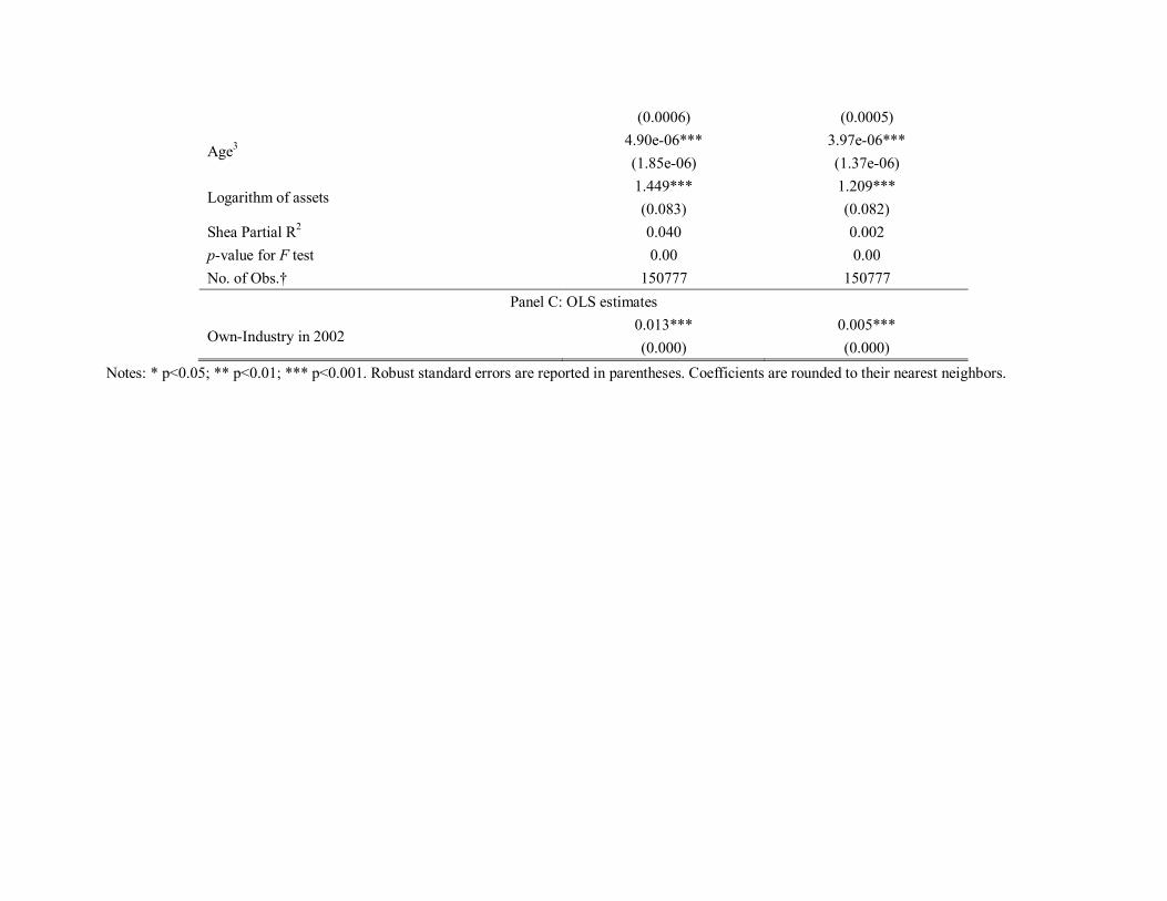
Furthermore, we conduct 2SLS regressions with firm/region-level data as a robustness check,

and the results are reported in Table 7.28,29 The 2SLS coefficient is 0.111, much higher than the

OLS coefficient 0.011 (see Table 2c), suggesting the same downward bias in the OLS estimate as

in the industry/region-level study. The signs of age variables still support Stigler’s (1951)

hypothesis mentioned earlier. These findings are also robust to the inclusion of related- and

other-industry neighboring employment.


6. Conclusion and Future Research

Using data from the U.S. Census of Manufacturers, Holmes (1999) finds a positive correlation

between geographic concentration and degree of vertical disintegration. China, the largest

developing economy in the world, has economic conditions very different from the U.S. We use

Chinese manufacturing data to replicate the work of Holmes (1999), and find the same

correlation between geographic concentration and vertical disintegration in China.

To investigate whether geographic concentration has a causal effect on vertical disintegration,

we next use population data from more than 80 years ago to instrument geographic concentration

27 Note that the 2SLS estimates using different instruments are asymptotically equivalent, but not necessarily equal. 28 In Table 7, we use dummy variables to control for two-digit- rather than four-digit-industry fixed effects, because regressions with 150,777 observations and 517 four-digit-industry dummy variables demand equipment that can do very intensive computing, to which we do not have access. 29 As the instrument (i.e., the cross-region population of China in 1920) is available only at the region level, these results should be interpreted with caution.

16

in China. Our estimates show that (1) geographic concentration has a positive and statistically

significant causal effect on the degree of vertical disintegration, and (2) the coefficient of

geographic concentration turns out to be much higher when endogeneity is treated. In other

words, geographic concentration actually has a stronger influence than previously expected.

Future research can expand upon the ideas presented in this paper in several ways. First, the

measure of vertical disintegration used in this study, as mentioned in Holmes (1999), “has

well-known inadequacies.” When data conditions permit, a study with other measures of vertical

disintegration should be undertaken. Second, future research should also examine whether the

effect of geographic concentration on vertical disintegration varies over time. Recent

technological developments are believed to be transforming the internal organization of firms

(Acemoglu et al., 2005). Thus, the role of geographic concentration is likely to change because

the importance of geographic concentration on vertical disintegration may wane in an idealized

“global village.”

Third, it will be interesting to investigate the relationship between the causality identified in

this paper and firm size, industrial structure, and corporate organization. Rosenthal and Strange

(2003, 2008) find that employment at small firms, compared to that at large firms, presents much

greater attraction to potential new arrivals, and creates a virtuous circle that favors the

entrepreneurial creation of more small establishments. Small firms can be either the outcome of

vertical disintegration, or the cause for vertical disintegration. Future research in this direction

may shed light on how external increasing return generates geographic concentration, which is a

fundamental question in urban economic discourse.

17

References Acemoglu, D., Aghion, P., Lelarge, C., Van Reenan, J., Fabrizio, Z., 2007a. Technology,

Information and the Decentralization of the Firm. Quarterly Journal of Economics 122(4), 1759-1799.

Acemoglu, D., Aghion, P., Griffith, R., Zilibotti, F., 2005. Vertical Integration and Technology: Theory and Evidence.

Acemoglu, D., Johnson, S., Mitton, T, 2007b. Determinants of Vertical Integration: Financial Development and Contracting Costs.

Acemoglu, D., Johnson, S., Robinson, J. A., 2001. The Colonial Origins of Comparative Development: An Empirical Investigation. American Economic Review 91 (5), 1369-1401.

Acemoglu, D., Johnson, S., Robinson, J. A., 2002. Reversal of Fortune: Geography and Institutions in the Making of the Modern World Income Distribution. Quarterly Journal of Economics 117 (4), 1231-1294.

Adelman, M. A., 1955. Concept of Statistical Measure of Vertical Integration, in: Stigler, G. J. (Ed.), Business Concentration and Price Policy. Princeton University Press, Princeton, MA.

Allen, G. C., 1929. The Industrial Development of Birmingham and the Black Country, 1860–1927. Allen and Unwin, London, United Kingdom.

Antràs, P., 2003. Firms, Contracts, and Trade Structure. Quarterly Journal of Economics 118, 1375-1418.

Antràs, P., 2006. Property Rights and the International Organization of Production. American Economic Review Papers and Proceedings 95 (2), 25-32.

Antràs, P., Helpman, E., 2004. Global Sourcing. Journal of Political Economy 112, 552-580. Antràs, P., Helpman, E., 2006. Contractual Frictions and Global Sourcing. NBER Working Paper

12747. Antràs, P., Garicano, L., Rossi-Hansberg, E., 2006. Offshoring in a Knowledge Economy.

Quarterly Journal of Economics 121 (1), 31-77. Au, C.-C., Henderson, V., 2002. How Migration Restrictions Limit Agglomeration and

Productivity in China. NBER Working Paper 8707. Bai, C.-E., Du, Y., Tao, Z., Tong, S. Y., 2004. Local Protectionism and Regional Specialization:

Evidence from China’s Industries. Journal of International Economics 63(2), 397-417. Baker, P., Hubbard, T. N., 2004. Contractibility and Asset Ownership: On-Board Computers and

Governance in US Trucking. Quarterly Journal of Economics 119 (4), 1443-1479. Chapman, S.J., Ashton, T.S., 1914. The Sizes of Businesses Mainly in the Textile Industries.

Journal of the Royal Statistical Society 77 (5), 469-555. Chen, Y., 2005. Vertical Disintegration. Journal of Economics and Management Strategy 14,

209-229. Chen, Y., Riordan, M., 2007. Vertical Integration, Exclusive Dealing, and ex post Cartelization.

RAND Journal of Economics 38, 1-21. Coase, R. H., 1937. The Nature of the Firm. Economica 4 (16), 386-405. Davis, D. R., Weinstein, D. E., 2002. Bones, Bombs, and Break Points: The Geography of

Economic Activity. American Economic Review 92 (5), 1269-1289.

18

Davis, D. R., Weinstein, D. E., 2003. Market Access, Economic Geography and Comparative Advantage: An Empirical Test. Journal of International Economics, 1-23.

Dinlersoz, E. M., 2004. Cities and the Organization of Manufacturing. Regional Science and Urban Economics 34(1), 71-100.

Duranton, G., Puga, D., 2001. Nursery Cities: Urban Diversity, Process Innovation, and the Life Cycle of Products. American Economic Review 91(5), 1454-1477.

Ellison, G., Glaeser, E. L., 1997. Geographic Concentration in U.S. Manufacturing Industries: A Dartboard Approach. Journal of Political Economy 105 (5), 889-927.

Eckard, E.W., 1979. A Note on the Empirical Measurement of Vertical Integration. Journal of Industrial Economics 28(1), 105-107.

Feenstra, R. C., Hanson, G. H., 2005. Ownership and Control in Outsourcing to China: Estimating the Property-Rights Theory of the Firm. Quarterly Journal of Economics 120 (2), 729-762.

Feenstra, R. C., 1998. Integration of Trade and Disintegration of Production in the Global Economy. Journal of Economic Perspectives 12 (4), 31-50.

Goldstein, G. S., Gronberg, T. J., 1984. Economies of Scope and Economies of Agglomeration. Journal of Urban Economics 16(1), 91-104.

Gort, M., 1962. Diversification and Integration in American Industry. Princeton University Press, Princeton, NJ.

Grossman, G., Helpman, E., 2002. Integration versus Outsourcing in Industry Equilibrium. Quarterly Journal of Economics 117 (1), 85-120.

Grossman, G., Helpman, E., 2004. Managerial Incentives and the International Organization of Production. Journal of International Economics 63 (2), 237-262.

Grossman, G., Helpman, E., 2005. Outsourcing in a Global Economy. Review of Economic Studies 72 (1), 135-159.

Grossman, S. J., Hart, O. D., 1986. The Costs and Benefits of Ownership: A Theory of Vertical and Lateral Integration. Journal of Political Economy 94 (4), 691-719.

Hall, M., 1959. Made in New York. Harvard University Press, Cambridge, MA. Hanson, G. H., 2005. Market Potential, Increasing Returns and Geographic Concentration.

Journal of International Economics 67 (1), 1-25. Hanson, G. H., Mataloni, R. J., Slaughter, M. J., 2005. Vertical Production Networks in

Multinational Firms." Review of Economics and Statistics 87 (4), 664-678. Hart, O., 1995. Firms, Contracts and Financial Structure. Oxford University Press, Oxford. Hart, O., Moore, J., 1990. Property Rights and the Nature of the Firm. Journal of Political

Economy 98 (6), 1119-1158. Helsley, R.W., Strange, W. C., 2002. Innovation and Input Sharing. Journal of Urban Economics

51(1), 25-45. Helsley, R.W., Strange, W. C., 2007. Agglomeration, Opportunism, and the Organization of

Production. Journal of Urban Economics 62(1), 55-75. Helpman, E., 2006. Trade, FDI, and the Organization of Firms. Journal of Economic Literature 44

(3), 589-630. Holmes, T.J., 1999. Localization of Industry and Vertical Disintegration. Review of Economics

19

and Statistics 81 (2), 314-325. Hortaçsu, A., C. Syverson, 2007. Cementing Relationships: Vertical Integration, Foreclosure,

Productivity, and Prices. NBER Working Paper 12894. Hummels, D., Ishii, J., Yi, K.-M., 2001. The Nature and Growth of Vertical Specialization in

World Trade. Journal of International Economics 54 (1), 75-96. Hummels, D., Rapoport, D., Yi, K.-M., 1998. Vertical Specialization and the Changing Nature of

World Trade. Economic Policy Review (Jun), 79-99. Joskow, P. L., 1987. Contract Duration and Relationship-Specific Investments: Empirical

Evidence from Coal Markets. American Economic Review 77 (1), 168-185. Keilbach, M., 2000. Spatial Knowledge Spillovers and the Dynamics of Agglomeration and

Regional Growth. Springer-Verlag New York Inc., New York, NY. Krugman, P., 1980. Scale Economies, Product Differentiation, and the Pattern of Trade. American

Economic Review 70 (5), 950-959. Krugman, P., 1991. Increasing Returns and Economic Geography. Journal of Political Economy

99 (3), 483-499. Krugman, P., A. Venables, 1995. Globalization and the Inequality of Nations. Quarterly Journal of

Economics 110 (4), 857-880. Laffer, A. B., 1969. Vertical Integration by Corporations, 1929-1965. Review of Economics and

Statistics 51 (1), 91-93. Levy, D., 1984. Testing Stigler's Interpretation of the Division of Labor is Limited by the Extent

of the Market. Journal of Industrial Economics 32 (3), 377-389. Lichtenberg, R., 1960. One-tenth of a Nation: National Forces in the Economic Growth of the

New York Region. Harvard University Press, Cambridge, MA. Lieberman, M. B., 1991. Determinants of Vertical Integration: An Empirical Test. Journal of

Industrial Economics 39 (5), 451-466. Lu, J., Tao, Z., 2006. Trends and Determinants of China’s Industrial Agglomeration. Journal of

Urban Economics, forthcoming. Marshall, A., 1920. Principles of economics. Macmillan and Co., Ltd., London, United Kingdom. Masten, S. E., 1984. The Organization of Production: Evidence from the Aerospace Industry.

Journal of Law and Economics 27 (2), 403-417. McLaren, J., 1999. Supplier Relations and the Market Context: A Theory of Handshakes. Journal

of International Economics 48 (1), 121-138. Monteverde, K., Teece, D. J., 1982. Supplier Switching Costs and Vertical Integration in the

Automobile Industry. Bell Journal of Economics 13 (1), 206-213. Murakami, N., Liu, D., Otsuka, K., 1996. Market Reform, Division of Labor, and Increasing

Advantage of Small-Scale Enterprises: The Case of the Machine Tool Industry in China. Journal of Comparative Economics 23 (3), 256-277.

National Bureau of Statistics of China, 2003. China Statistical Yearbook 2003. China Statistics Press, Beijing, China.

Perry, M., 1989. Vertical Integration: Determinants and Effects, in: Schmalensee R., Willig, R.D. (Eds.), Handbook of Industrial Organization, Elsevier Science Publishers B.V., New York,

20

NY. 183-255. Picard, P. M., Zeng, D.-Z., 2005. Agricultural Sector and Industrial Agglomeration. Journal of

Development Economics 77(1), 75-106. Poncet, S., 2003. Measuring Chinese Domestic and International Integration. China Economic

Review 14, 1-21 Puga, D., Trefler, D., 2002. Knowledge Creation and Control in Organizations. NBER Working

Paper 9121. Rosenthal, S.S., Strange, W.C., 2001. The Determinants of Agglomeration. Journal of Urban

Economics 50(2), 191-229. Rosenthal, S.S., Strange, W.C., 2003. Geography, Industrial Organization, and Agglomeration.

Review of Economics and Statistics 85(2), 377-393. Rosenthal, S.S., Strange, W.C., 2004. Evidence on the Nature and Sources of Agglomeration

Economies, in Henderson V., Thisse, J. (Eds.), Handbook of Urban and Regional Economics, Volume 4. Elsevier Science Publishers B.V., New York, NY.

Rosenthal, S.S., Strange, W.C., 2005. The Geography of Entrepreneurship in the New York Metropolitan Area.

Rosenthal, S.S., Strange, W.C. 2006. The Micro-Empirics of Agglomeration Economies, in: Arnott, D., McMillen, P. (Eds.), A Companion to Urban Economics (Blackwell Companions to Contemporary Economics). Wiley-Blackwell, Malden, MA.

Rosenthal, S.S., Strange, W.C. 2008. Small Establishments/Big Effects: Agglomeration, Industrial Organization and Entrepreneurship.

Scott, A.J., 1988. Metropolis. University of California Press, Berkley, CA. Scott, A.J., 2000. The Cultural Economy of Cities. Sage Publications, London, United Kingdom. Scott, A. J., Kwok, E. C., 1989. Inter-Firm Subcontracting and Locational Agglomeration: A Case

Study of the Printed Circuits Industry in Southern California. Regional Studies 25, 405-416. Smith, Adam, 1776. The Wealth of Nations, reprinted in 1976. University of Chicago Press,

Chicago, IL. Special Committee on Survey and Occupation of China Continuation Committee, 1987. Statistics

of China Christianism (revised edition by Chinese Academy of Social Sciences): 1901-1920. Chinese Academy of Social Sciences Press, Beijing, China.

Spencer, B. J., 2005. International Outsourcing and Incomplete Contracts. Canadian Journal of Economics 38(4), 1107-1135.

Stigler, G. J., 1951. The Division of Labor is Limited by the Extent of the Market. Journal of Political Economy 59 (3), 185-193.

Strange, W.C., 2005. Urban Agglomeration. Prepared for the New Palgrave Dictionary of Economics, 2nd Ed.

Tucker, I. B., Wilder, R. P., 1977. Trends in Vertical Integration in the U.S. Manufacturing Sector. Journal of Industrial Economics 26 (1), 81-94.

U.S. Department of Justice, 1985. Guidelines for Vertical Restraints, reprinted as a Special Supplement in Antitrust Trade and Regulation Report, No. 1199, January 24, 1985, 48, 3-12.

Wen, M., 2004. Relocation and Agglomeration of Chinese Industry. Journal of Development

21

Economics 73(1), 329-347. Williamson, O. E., 1975. Markets and Hierarchies: Analysis and Antitrust Implications. Free

Press, New York, NY. Williamson, O. E., 1985. The Economic Institutions of Capitalism. Free Press, New York, NY. Yang, X., Ng, Y.-K., 1993. Specialization and Economic Organization. North-Holland,

Amsterdam. Young, A.A., 1928. Increasing Returns and Economic Progress. Economic Journal 38 (152),

527-542. Young, A., 2000. The Razor’s Edge: Distortions and Incremental Reform in the People’s Republic

of China. Quarterly Journal of Economics 115(4), 1091-1135. Zhang, Y., 2004. Vertical Specialization of Firms: Evidence from China’s Manufacturing Sector.

University of Pittsburgh Working Paper.

22

TABLE 1: DESCRIPTIVE STATISTICS

Description Mean Std.Dev. Min. Max. Panel A: Summary Statistics of Employment-Weighted Variables

PII х 100 80.7 10.46 5.8 100 Neighboring Employment (1,000 employees)

Own-Industry 3.4 13.29 0 536.0 Related-Industry 76.7 106.79 0 820.9 Other-Industry 1651.7 1503.58 11.2 5776.6

Panel B: Summary Statistics of Output-Weighted Variables

PII х 100 81.1 10.82 5.8 100 Neighboring Employment (1,000 employees)

Own-Industry 3.4 13.35 0 536.3 Related-Industry 76.7 106.79 0 820.9 Other-Industry 1651.7 1503.58 11.2 5776.6

Panel C: Other

Population in 1920 (1,000 persons) 18486.1 13605.67 1054.8 60129.4 No. of firms in (i,a) 15.0 42.876 1 1682

No. of 4-digit China SIC industries 518 No. of 2-digit China SIC industries 29

No. of regions (provinces) 31

TABLE 2A: OLS RESULTS IN HOLMES (1999) Data: U.S. Census 1987 Level: Industry/Region

Model

Own-Industry Related-Industry Other-Industry

R2 Level

(1,000) Level

squared Level cubic

Level (1,000)

Level squared

Level cubic

Level (1,000)

Level squared

Level cubic

1 0.04

(0.01) 0.001

2 0.04

(0.02)

0.000 (0.003)

0.001

3 0.05

(0.02)

0.009 (0.004)

-0.0013 (0.0004)

0.002

4 0.35

(0.07) -0.013 (0.003)

0.00012 (0.00004)

-0.054 (0.023)

0.0009 (0.0003)

-3.0e-6 (1.2e-6)

0.0025 (0.0032)

-1.4e-5 (0.7e-5)

1.0e-8 (0.4e-8)

0.006

Note: This table is a duplicate of the first panel of Table 3 in Holmes (1999). Asterisks are not reported in the original table.

TABLE 2B: OLS RESULTS Data: China NSBED 2002

Level: Industry/Region

Model

Own-Industry Related-Industry Other-Industry Weighted

by R2 Level

(1,000) Level

squared Level cubic

Level (1,000)

Level squared

Level cubic

Level (1,000)

Level squared

Level cubic

1 0.017*** (0.001)

Employment 0.029

2 0.011*** (0.001)

0.008*** (0.0004)

Employment 0.071

3 0.005*** (0.001)

0.002*** (0.001)

0.0008*** (0.00004)

Employment 0.105

4 0.020*** (0.005)

-0.00009*** (0.00003)

1.15e-07*** (4.00e-08)

0.019*** (0.003)

-0.00005***

(9.49e-06)

4.22e-08***

(8.59e-09)

0.001** (0.0004)

-1.67e-07 (1.32e-07)

1.59e-11 (1.47e-11)

Employment 0.111

5 0.019*** (0.001)

Output 0.029

6 0.013*** (0.001)

0.010*** (0.0004)

Output 0.072

7 0.006*** (0.001)

0.002*** (0.001)

0.0008*** (0.00004)

Output 0.106

8 0.029*** (0.006)

-150.1*** (34.9)

2.00e-07*** (4.96e-08)

0.021*** (0.003)

-0.00006***

(0.00001)

4.39e-08***

(9.51e-09)

0.001** (0.0004)

-2.03e-07 (1.43e-07)

2.36e-11 (1.60e-11)

Output 0.113

Notes: * p<0.05; ** p<0.01; *** p<0.001. Robust standard errors are reported in parentheses. Coefficients are rounded to their nearest neighbors.

TABLE 2C: OLS RESULTS Data: China NSBED 2002

Level: Firm/Region

Model Own-Industry Related-Industry Other-Industry

Age Age2 Age3 Logarithm of assets

R2 Level (1,000)

Level squared

Level Cubic

Level (1,000)

Level squared

Level Cubic

Level (1,000)

Level squared

Level Cubic

1 0.013***

(0.000)

-0.051***

(0.007)

0.0003**

(0.0001)

-9.11e-07***

(3.48e-07)

-0.587***

(0.020) 0.12

2 0.011***

(0.000)

0.008***

(0.000)

-0.042***

(0.007)

0.0003**

(0.0001)

-8.92e-07**

(3.56e-07)

-0.592***

(0.020) 0.13

3 0.005***

(0.000)

0.002***

(0.000)

0.001***

(0.000)

-0.033***

(0.007)

0.0003**

(0.0001)

-9.66e-07***

(3.72e-07)

-0.609***

(0.020) 0.14

4 0.035***

(0.002)

-0.0001***

(0.0000)

1.51e-07***

(1.38e-08)

0.005***

(0.002)

-0.00001***

(4.90e-06)

1.33e-08***

(4.34e-09)

0.0008***

(0.0002)

1.38e-07

(8.66e-08)

-2.72e-11***

(9.07e-12)

-0.031***

(0.007)

0.0003**

(0.0001)

-9.76e-07***

(3.75e-07)

-0.622***

(0.020) 0.14


TABLE 3: 2SLS RESULTS Level: Industry/Region

Model 1 2

Employment weighted Output weighted

Panel A: Second stage (dependent variable: PII)

Own-industry neighboring employment in 2002 0.079*** (0.004)

0.098*** (0.005)

Panel B: First stage (dependent variable: own-industry neighboring employment in 2002)

Logarithm of population in 1920 1.754*** (0.057)

1.555*** (0.055)

Shea Partial R2 0.088 0.075

p-value for F test 0.000 0.000

No. of Obs. 9939 9939

Panel C: OLS estimates


0.019*** (0.001)


TABLE 4: ROBUSTNESS CHECK I: SUB-SAMPLE Level: Industry/Region

Model 1 2




0.796*** (0.101)



0.139*** (0.006)



No. of Obs. 2987 2987


TABLE 5: ROBUSTNESS CHECK II: POPULATION SCALE EFFECT Level: Industry/Region

Model 1 2




0.109*** (0.017)

Related-industry neighboring employment in 2002 0.002*** (0.0006)

0.003*** (0.0008)

Other-industry neighboring employment in 2002 -0.0001 (0.0002)

-0.0003 (0.0002)



0.550*** (0.062)

Related-industry neighboring employment in 2002 0.002

(0.005) -0.006 (0.005)

Other-industry neighboring employment in 2002 0.010*** (0.0004)

0.010*** (0.0004)



No. of Obs. 9939 9939


TABLE 6: ROBUSTNESS CHECK III: ALTERNATIVE IV Level: Industry/Region

Model 1 2


Panel A: 2SLS estimates, the second stage (dependent variable: PII)


0.010*** (0.003)


0.003*** (0.001)


0.0009*** (0.0001)

No. of Obs. 10129 10129

Panel B: OLS estimates (dependent variable: PII)


0.006*** (0.001)


0.002*** (0.001)


0.0008*** (0.00004)

No. of Obs. 10129 10129

Notes: * p<0.05; ** p<0.01; *** p<0.001. Robust standard errors are reported in parentheses. Coefficients are rounded to their nearest neighbors. The first-stage results are not reported due to space limit, but available upon request.

TABLE 7: ROBUSTNESS CHECK IV: BRANCH-LEVEL STUDY Level: Firm/Region

Model 1 2



0.179*** (0.016)

Related-industry neighboring employment in 2002 0.008***

(0.0007)

Other-industry neighboring employment in 2002 -0.001***

(0.0002)

Age -0.034***

(0.007) -0.037***

(0.008)

Age2 0.0005*** (0.0002)

0.0006*** (0.0002)

Age3 -1.47e-06*** (4.34e-07)

-1.68e-06*** (4.82e-07)

Logarithm of assets -0.752***

(0.022) -0.823***

(0.031) Panel B: First stage (dependent variable: own-industry neighboring employment in 2002)


3.25*** (0.15)

Related-Industry neighboring employment in 2002 -0.037***

(0.002)

Other-Industry neighboring employment in 2002 0.011***

(0.0001)

Age -0.120***

(.026) 0.015

(0.025) Age2 -0.0013** -0.0016***

(0.0006) (0.0005)

Age3 4.90e-06*** (1.85e-06)

3.97e-06*** (1.37e-06)

Logarithm of assets 1.449*** (0.083)

1.209*** (0.082)

Shea Partial R2 0.040 0.002 p-value for F test 0.00 0.00 No. of Obs.† 150777 150777

Panel C: OLS estimates

Own-Industry in 2002 0.013*** (0.000)

0.005*** (0.000)


FIGURE 1: IDENTIFICATION STRATEGY

020

0000

040

0000

060

0000

0C

once

ntra

tion

0 20000 40000 60000 80000 100000Population(in 1,000)

FIGURE 2: GEOGRAPHIC CONCENTRATION AND POPULATION

050

000

1000

00Po

pula

tion

in 2

002

(in 1

,000

)

0 20000 40000 60000Population in 1920 (in 1,000)

FIGURE 3: HISTORICAL AND CURRENT POPULATIONS

FIGURE 4: ESTIMATED COEFFICIENTS ACROSS 518 FOUR-DIGIT INDUSTRIES

geographic concentration and vertical disintegration ... · geographic concentration and vertical...

Documents