ER

DC

/G

RL T

R-2

0-5

Geointelligence – Geospatial Data Analysis and Decision Support

Local Spatial Dispersion for Multiscale

Modeling of Geospatial Data

Exploring Dispersion Measures to Determine Optimal Raster Data Sample Sizes

Ge

os

pa

tia

l R

es

ea

rch

La

bo

rato

ry

S. Bruce Blundell and Nicole M. Wayant February 2020

Approved for public release; distribution is unlimited.

The U.S. Army Engineer Research and Development Center (ERDC) solves

the nation’s toughest engineering and environmental challenges. ERDC develops

innovative solutions in civil and military engineering, geospatial sciences, water

resources, and environmental sciences for the Army, the Department of Defense,

civilian agencies, and our nation’s public good. Find out more at www.erdc.usace.army.mil.

To search for other technical reports published by ERDC, visit the ERDC online library

at https://erdc-library.erdc.dren.mil.

Geointelligence – Geospatial Data Analysis

and Decision Support

ERDC/GRL TR-20-5

February 2020

Local Spatial Dispersion for Multiscale

Modeling of Geospatial Data

Exploring Dispersion Measures to Determine Optimal Raster Data Sample Sizes

S. Bruce Blundell and Nicole M. Wayant

Geospatial Research Laboratory

U.S. Army Engineer Research and Development Center

7701 Telegraph Road

Alexandria, VA 22315-3864

Final Report

Approved for public release; distribution is unlimited.

Prepared for Headquarters, U.S. Army Corps of Engineers

Washington, DC 20314-1000

Under PE 62784/Project 855/Task 22 “New and Enhanced Tools for Civil-Military

Operations”

ERDC/GRL TR-20-5 ii

Abstract

Scale, or spatial resolution, plays a key role in interpreting the spatial

structure of remote sensing imagery or other geospatially dependent data.

These data are provided at various spatial scales. Determination of an

optimal sample or pixel size can benefit geospatial models and

environmental algorithms for information extraction that require multiple

datasets at different resolutions. To address this, an analysis was

conducted of multiple scale factors of spatial resolution to determine an

optimal sample size for a geospatial dataset. Under the NET-CMO project

at ERDC-GRL, a new approach was developed and implemented for

determining optimal pixel sizes for images with disparate and

heterogeneous spatial structure. The application of local spatial dispersion

was investigated as a three-dimensional function to be optimized in a

resampled image space. Images were resampled to progressively coarser

spatial resolutions and stacked to create an image space within which

pixel-level maxima of dispersion was mapped. A weighted mean of

dispersion and sample sizes associated with the set of local maxima was

calculated to determine a single optimal sample size for an image or

dataset. This size best represents the spatial structure present in the data

and is optimal for further geospatial modeling.

DISCLAIMER: The contents of this report are not to be used for advertising, publication, or promotional purposes.

Citation of trade names does not constitute an official endorsement or approval of the use of such commercial products.

All product names and trademarks cited are the property of their respective owners. The findings of this report are not to

be construed as an official Department of the Army position unless so designated by other authorized documents.

DESTRUCTION NOTICE – Destroy by any method that will prevent disclosure of contents or

reconstruction of the document.

ERDC/GRL TR-20-5 iii

Contents

Abstract .......................................................................................................................................................... ii

Figures and Tables ........................................................................................................................................ iv

Preface ............................................................................................................................................................. v

1 Introduction ............................................................................................................................................ 1

1.1 Background ..................................................................................................................... 1

1.2 Objectives ........................................................................................................................ 3

1.3 Approach ......................................................................................................................... 3

2 Methods .................................................................................................................................................. 5

2.1 Overview .......................................................................................................................... 5

2.2 Algorithmic approach ...................................................................................................... 6

2.3 Algorithm development .................................................................................................. 8

2.3.1 Hessian matrix optimization ............................................................................................... 8

2.3.2 Peakedness and optimal sample size .............................................................................. 11 2.4 Graphical user interface development ........................................................................ 13

3 Data ....................................................................................................................................................... 16

4 Results ..................................................................................................................................................18

4.1 Florida WorldView2 dataset ......................................................................................... 19

4.2 Cambodia tree cover dataset ....................................................................................... 21

4.3 Cambodia population density dataset ......................................................................... 24

4.4 Cambodia precipitation dataset .................................................................................. 27

5 Discussion ............................................................................................................................................ 30

6 Summary and Conclusions ............................................................................................................... 32

References ................................................................................................................................................... 33

Acronyms and Abbreviations .................................................................................................................... 34

Report Documentation Page

ERDC/GRL TR-20-5 iv

Figures and Tables

Figures

Figure 1. Spatial data model. ....................................................................................................................... 5

Figure 2. Local spatial dispersion analysis tool. ...................................................................................... 13

Figure 3. WorldView2 image (Florida). ....................................................................................................... 16

Figure 4. Tree cover data (Cambodia). ...................................................................................................... 16

Figure 5. Population density data (Cambodia). ........................................................................................ 17

Figure 6. Precipitation data (Cambodia). .................................................................................................. 17

Figure 7. Mean, median MAD vs. sample size (WorldView2 dataset). .................................................. 19

Figure 8. Number of Local maxima vs. sample size (WorldView2 dataset). ........................................ 20

Figure 9. Local maxima distribution at sample size 2.6 m (WorldView2 dataset). ............................. 20

Figure 10. Local maxima distribution in LSD space (WorldView2 dataset). ........................................ 21

Figure 11. Mean, median MAD vs. sample size (Cambodia tree cover dataset). ............................... 22

Figure 12. MAD heat map at sample size 89 m (Cambodia tree cover dataset). ............................... 22

Figure 13. Local maxima distribution, sample size 89 m (Cambodia tree cover

dataset). ..................................................................................................................................... 23

Figure 14. Peakedness histogram (Cambodia tree cover dataset). ...................................................... 23

Figure 15. Mean, median MAD vs. sample size (Cambodia population dataset). .............................. 24

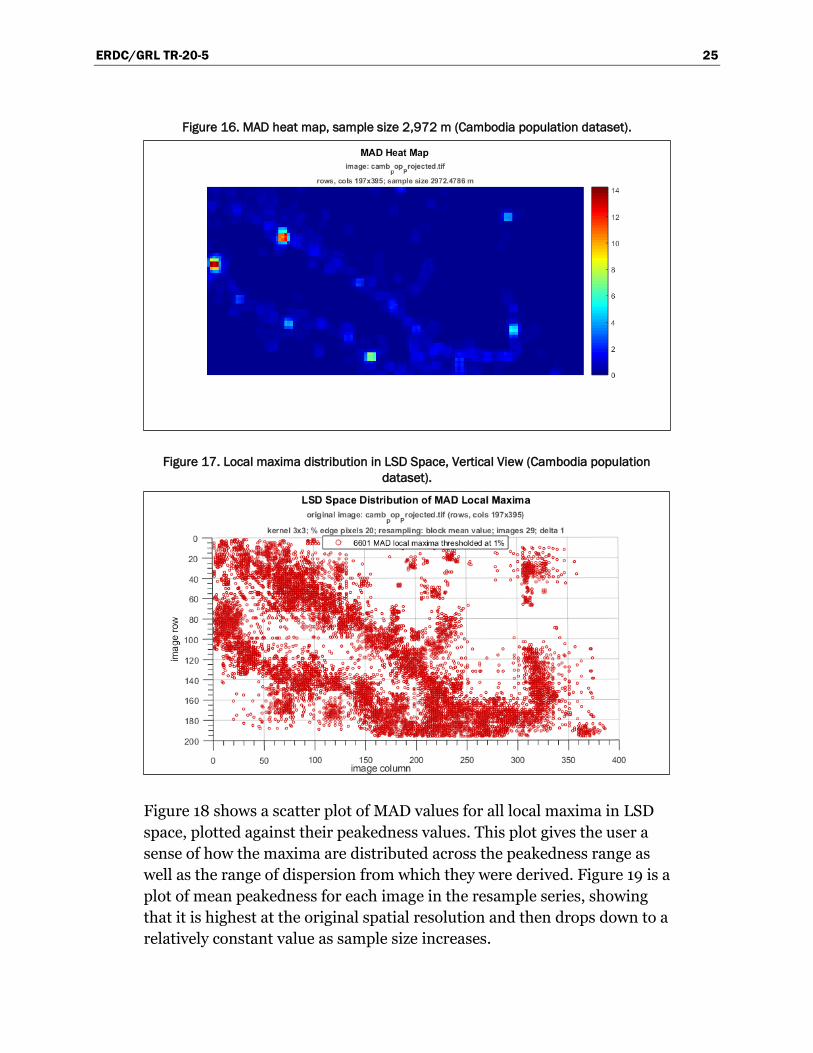
Figure 16. MAD heat map, sample size 2,972 m (Cambodia population dataset). ........................... 25

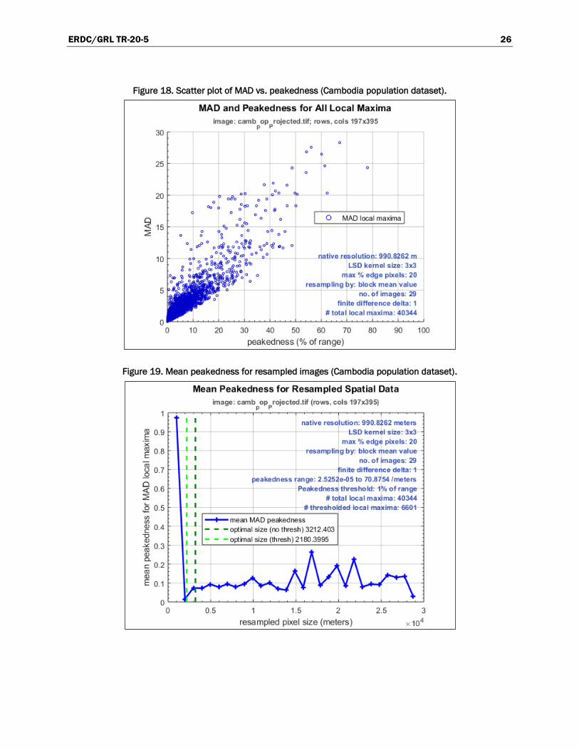
Figure 17. Local maxima distribution in LSD Space, Vertical View (Cambodia

population dataset). ................................................................................................................. 25

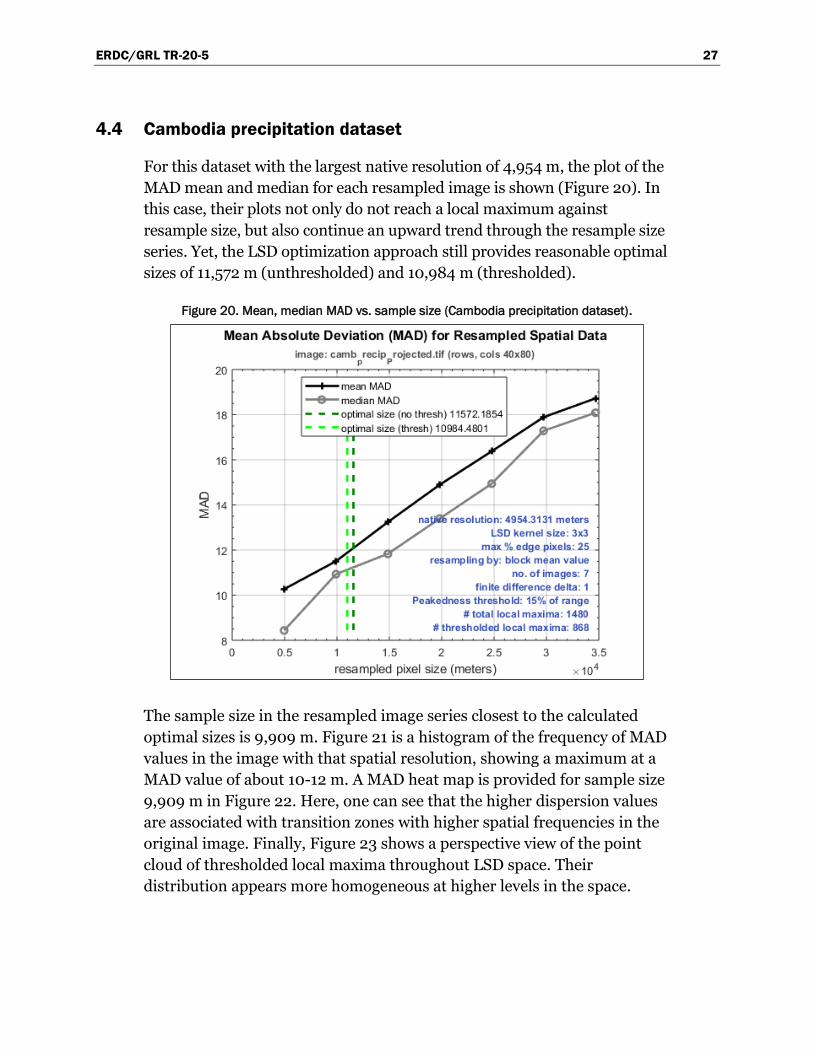
Figure 18. Scatter plot of MAD vs. peakedness (Cambodia population dataset). .............................. 26

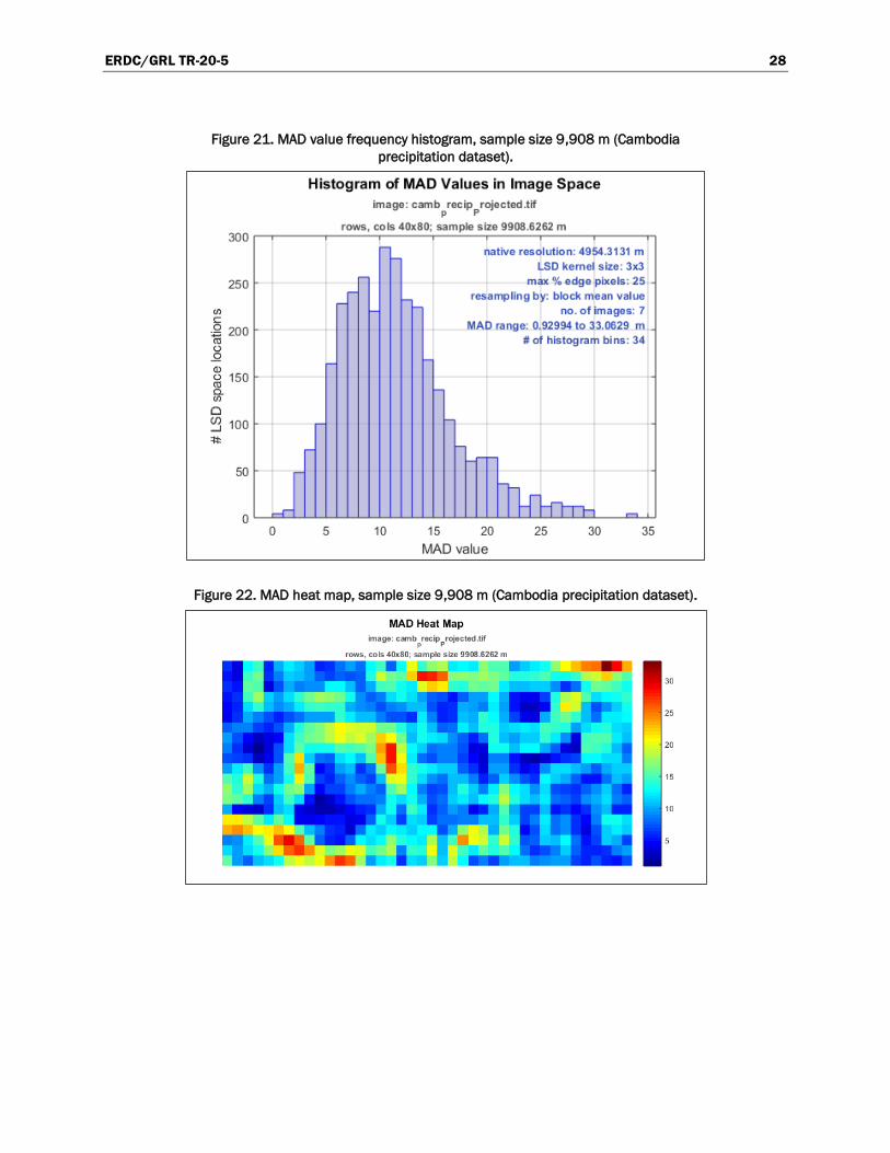
Figure 19. Mean peakedness for resampled images (Cambodia population dataset). .................... 26

Figure 20. Mean, median MAD vs. sample size (Cambodia precipitation dataset). .......................... 27

Figure 21. MAD value frequency histogram, sample size 9,908 m (Cambodia

precipitation dataset). .............................................................................................................. 28

Figure 22. MAD heat map, sample size 9,908 m (Cambodia precipitation dataset). ........................ 28

Figure 23. Local maxima distribution in LSD space (Cambodia precipitation dataset). .................... 29

Tables

Table 1. Dataset parameters and optimal sizes. ..................................................................................... 18

ERDC/GRL TR-20-5 v

Preface

This study was conducted for the Geospatial Research Laboratory (GRL)

under PE 62784/Project 855/Task 22, “NET-CMO.” The technical monitor

was Ms. Nicole Wayant.

The work was performed by the Data and Signature Analysis Branch (TR-

S) of the TIG Research Division (TR), U.S. Army Engineer Research and

Development Center, Geospatial Research Laboratory (ERDC-GRL). At

the time of publication, Ms. Jennifer L. Smith was Chief, TR-S;

Ms. Martha Kiene was Chief, TR; and Mr. Terrance Westerfield, TV-T was

the Technical Director for ERDC-GRL. The Deputy Director of ERDC-GRL

was Ms. Valerie L. Carney and the Director was Mr. Gary Blohm.

COL Teresa A. Schlosser was Commander of ERDC, and Dr. David W.

Pittman was the Director.

ERDC/GRL TR-20-5 vi

ERDC/GRL TR-20-5 1

1 Introduction

1.1 Background

Terrestrial features in remotely sensed imagery or geospatial data have

inherent and quantifiable spatial variability and heterogeneity. The spatial

resolution of a remotely sensed image represents the scale of sensor

observations on the land surface (i.e. the pixel size). Other types of spatially

sampled environmental data (e.g. precipitation) can be represented in

gridded or raster form. The selection of an appropriate scale depends on the

type of information desired as well as the size and variability of the land

phenomena under examination. In modeling processes on the Earth’s

surface, the spatial resolution must be considered. If the process is affected

by detail at a finer scale than provided by the data, the model’s output will

be misleading (Goodchild 2011).

The relationship between the size of objects or features in an image and

spatial resolution helps determine the spatial structure of the image. Fine

resolution, relative to scene object size, results in high correlation of

neighboring pixels, reducing the local spatial variance. Large pixel size,

relative to scene objects, results in a mixing of response from different

kinds of objects, also depressing local variance. The pixel size that results

in a maximum variance would then best capture the spatial variation in

the image (Rahman et al. 2003; McCloy and Bøcher 2007). As will be seen

in this study, this general principle may not hold for images with

heterogeneous spatial structure having a broad range of spatial frequency

of variation for image objects.

Understanding how an image and the features in it change as the spatial

resolution changes may allow for more efficient information extraction.

Yet, there is no generally recognized procedure for choosing an optimal

pixel size. Curran (2000) suggests that in classifying land cover by remote

sensing, results that are more accurate will be obtained if the spatial

resolution is similar to the size of a typical field. Using the local variance

approach, Woodcock and Strahler (1987) examined simulated images of

discrete land surface objects and found that a peak in a plot of local

variance against pixel size occurs at a range of ½ to ¾ of the object size.

Rahman et al. (2003) concluded that half the sample size associated with

the lowest peak was optimal for the vegetation types under study with

ERDC/GRL TR-20-5 2

hyperspectral data, as it agreed with semivariogram analysis and retained

characteristic spatial variation. This approach would seem to agree with

sampling theory as applied to digital images (Richards and Jia 1999).

However, McCloy and Bøcher (2007) found that the sample size associated

with the first trough in the local variance function is associated with the

highest classification accuracy for agricultural and forested scenes with

3-band imagery in the visible range. Choosing the sample size associated

with the peak introduced additional within-class variance, lowering the

classification accuracy.

Selection of a particular pixel for terrestrial land surface mapping or

modelling represents a sampling strategy in remote sensing. Careful

selection of an optimal sample size can enhance the precision of

measurement (Atkinson and Curran 1995). Marceau et al. (1994) defined

optimal spatial resolution as the sampling unit that corresponds to the

scale and aggregation level characteristic of the geographical entity under

consideration. The authors define the aggregation level as the degree to

which an earth surface feature is an assemblage of sub-elements. For

example, a tree is an aggregate of leaves, branches, and bark in a particular

arrangement. For a remote sensing image, the sampling unit is

represented by the resolution cell.

While increasing the resolution of geospatial data can provide more

information about its intrinsic subtle patterns, it can also make it more

difficult to model them accurately due to noise (Costanza and Maxwell

1994). Rahman et al. (2003) assessed image spatial structure of similar

vegetation by analyzing the mean local variance of pixel values at varied

spatial resolutions. The authors found that a maximum value for this

function may be related to an optimum pixel size for the segmentation of a

particular land surface process or feature type. Two competing concerns

are involved: finding a balance between reducing the correlation among

neighboring pixels having sizes smaller than the spatial structure, and

reducing effects of different spatial objects intermixed within a given pixel

(pixel mixing). The balance between these concerns is obtained by finding

the sample size associated with the maximum mean local variance of a

feature when plotted against pixel size (Woodcock and Strahler 1987). This

size will be tuned to the particular spatial structure of scene elements that

make up the feature or features under investigation.

ERDC/GRL TR-20-5 3

Whatever the strategy for choosing an optimal pixel size, the approach may

be suited to an image or image subset containing a dominant feature with a

characteristic spatial structure, but may not be effective for a scene with

multiple disparate features (e.g. mixed land cover types). In that case, the

spatial variance may not show a clear maximum as a function of spatial

resolution due to the mixing of a range of frequencies of spatial variation in

the scene. In this work, we build upon the literature to provide a method to

optimize the sample size of a geospatial dataset. Unlike previous research,

this method provides an optimal pixel size regardless of the heterogeneity of

the land surface features or geospatial data under consideration.

1.2 Objectives

This study is directly supporting the New and Enhanced Tools for Civil-

Military Operations (NET-CMO) project at the Engineer Research and

Development Center – Geospatial Research Laboratory (ERDC-GRL).

NET-CMO is concerned with the prediction and mapping of the spread of

disease across space and time by mosquito vectors. In epidemiology, land

cover, as derived from remote sensing, can be a critical variable in

assessing vector density and risk of disease (Curran et al. 2000). The

algorithms employed in the NET-CMO project require disparate spatial

datasets with a wide range of spatial resolutions that must be reconciled

through multiscale modeling techniques. Accordingly, the objective is to

devise a semi-automated method and workflow to determine the optimal

sample size for geospatial analysis and modelling within this project. To

address this objective, the role of local variance was examined in the

estimation of an optimal sample size for spatial data containing

environmental information. In this work, the term “sample size” is used to

indicate the pixel size that results from a particular level of image

resampling. A methodology was devised to select a spatial resolution that

will maximize the strength of the relationship between the sampled data in

an image and the biophysical variables of interest.

1.3 Approach

For any image or image subset with a relatively uniform spatial structure

or frequency of variation, measures of local variance often reach a

maximum at some level of resampling, and this sample size may be

optimal for various image or data processing functions. For many real-

world raster datasets with a heterogeneous spatial structure, this ideal

situation may not hold. When this happens, local variance can lose its

ERDC/GRL TR-20-5 4

value as an indicator for optimal sample size. In light of these difficulties, a

new approach was designed to the problem through multidimensional

analysis of resampled images with increasingly coarser spatial resolution.

A three-dimensional image space of resampled images was created and

Local Spatial Dispersion (LSD) throughout this space was calculated. As

used here, dispersion is a measure of the statistical distribution of image

values in some local neighborhood. Dispersion is represented by two

dispersion statistics: Local Spatial Variance (LSV) and Mean Absolute

Deviation (MAD). This “LSD space” was then optimized to create a set of

LSD local maxima, representing a subset of all LSD space locations. Rather

than seeking an elusive single maximum value of the local variance

function, the image sample sizes associated with the set of LSD space

locations of the local maxima in a weighted mean formulation were used to

arrive at an optimal sample size for the image under study. In this way, the

locality of variance throughout the multidimensional image space is

preserved and used to compute an optimal sample size for the dataset.

ERDC/GRL TR-20-5 5

2 Methods

In pursuit of our objectives, an algorithmic approach was developed that

addressed the creation of a spatial data model and a set of methods for

performing internal calculations to arrive at an optimal sample size. These

methods were required to compute and optimize LSD within the model

before calculating the optimal sample size based on the discovered set of

local maxima. A graphical user interface was then created in the MATLAB

software environment to perform the calculations and display the results

of LSD optimization.

2.1 Overview

Consider a three-dimensional model for spatial data with the image space

(row and column) comprising two independent dimensions and a third

dimension represented by the pixel aggregation level of the dataset’s

native resolution, or original sample size (Figure 1). The LSD of image

values for a particular dataset will vary throughout this spatial data model

and occupies what may be called “LSD space”.

Figure 1. Spatial data model.

LSD tells us how the local distribution of image values change as the image

location changes. A good choice for measuring LSD is LSV, but there are

other options, such as MAD. MAD is similar to LSV except the absolute

value is taken of the residuals rather than squaring them. Whatever the

dispersion statistic used, LSD values will vary across any particular image

according to the distribution of feature objects and their associated spatial

frequencies in the image or dataset. They will also vary in the orthogonal

direction for sample size at any image location. LSD can then be

represented in general as the trivariate function

ERDC/GRL TR-20-5 6

LSD = f(r,c,s)

where

r = row

c = column

s = sample size.

This multidimensional function cannot be easily represented visually and

must be estimated numerically. However, LSD space can be imagined as a

series of undulating surfaces stacked on top of each other, one for each

level of pixel aggregation of the spatial data’s native resolution. Any one of

these surfaces may have local maxima or minima due to the response of

LSD to particular spatial frequency regimes encountered at different

locations in LSD space. The authors are particularly interested in finding a

set of LSD local maxima, located throughout the multidimensional model,

for a chosen image or spatial dataset. A spatial dispersion maximum can

occur at a particular pixel aggregation level for a particular uniform

feature with an associated spatial frequency. The total set of these LSD

maxima values may allow us to determine an optimal sample or support

size for more efficient image segmentation, or provide a basis for

determining a uniform support size required by higher-level multiscale

modeling algorithms for spatial data.

2.2 Algorithmic approach

The first step in the process is to create the spatial data model by

populating it with resampled versions of the original image or spatial

dataset with progressively lower spatial resolution. To do this, a

resampling method must be chosen to create these pixel aggregation levels

calculated by a neighborhood function. Three resampling methods were

allowed: block processing of the mean of each set of neighborhood values,

bilinear interpolation, and bicubic interpolation.

Next, compute the local dispersion at each cell location for each resampled

image in the spatial data model. As mentioned previously, common

techniques for this purpose include LSV and MAD. The result is a set of

LSD “images,” each one having the spatial resolution of the resampled

image from which it was created. However, in order to proceed further

with the matrix algebra necessary to find the set of LSD maxima in this

multidimensional space, the spatial data model must have uniform

ERDC/GRL TR-20-5 7

granularity along all three orthogonal directions (r,c,s). This is required in

order to have a uniform distribution of LSD values. Due to the nature of

the pixel aggregation process, this granularity decreases in the sample size

(s) direction. Therefore, an interpolation scheme must be applied to each

LSD image to achieve the same spatial resolution as the original image.

Nearest neighbor interpolation will be employed for this purpose. This will

result in a uniform distribution of LSD values throughout LSD space.

In order to find the complete set of LSD maxima, the multidimensional

function LSD = f(r,c,s) must be optimized. Optimization strategies can be

classified into two groups depending on whether they require evaluation of

derivatives. Direct methods are those that do not require such

calculations; gradient methods are those that do (Chapra and Canale

2002). A gradient method involving a matrix of second-order partial

derivatives known as the Hessian matrix will be employed. This symmetric

matrix will have one row and column for each independent variable. The

procedure will be as follows: the original dataset will first be successively

re-sampled to provide the sample size dimension in LSD space. At each

level of resampling, LSD will be calculated for each row, column location.

The elements of the Hessian matrix H will then be evaluated by finite-

difference approximation for each LSD space location. For each 3-element

vector x=x(r,c,s) in LSD space, a particular series of determinants will be

computed based on three subsets of H. These determinants will allow us to

test the Hessian for a property known as negative definiteness. Describing

this property involves consideration of other concepts in linear algebra

and they will not be pursued further here. For the purposes of this report,

it can be shown that x will be a local maximum of f(r,c,s) if H(x) is

negative definite. The test for negative definiteness will involve the second

partial derivatives with respect to each variable, as well as the mixed

partials with respect to any two of the three variables.

The result will be a set of x vectors that provides the sample size, s,

associated with each local maximum of f(r,c,s) in the dataset. A weighted

average of these values can then be made based on the pixel aggregation

level associated with the sample size. This average will be taken as the

optimal sample size for the image or dataset under study.

ERDC/GRL TR-20-5 8

2.3 Algorithm development

2.3.1 Hessian matrix optimization

Let us first define the Hessian matrix for the three independent variables:

row (r), column (c), and sample size (s):

h11 h12 h13 ∂2f/∂r2 ∂2f/∂r∂c ∂2f/∂r∂s

Hrcs = h21 h22 h23 = ∂2f/∂c∂r ∂2f/∂c2 ∂2f/∂c∂s

h31 h32 h33 ∂2f/∂s∂r ∂2f/∂s∂c ∂2f/∂s2

In order to find the Hessian for each x vector, each element must be

evaluated numerically. A finite divided-difference approximation method

will be used for this purpose. The values of x in the row, column, and

sample dimensions will be perturbed by some small fractional value, δ, to

generate the partial derivatives. δ cannot be too small or too large. Too

small a value may not provide enough variation in the variable to capture

the functional trend at that location. Too large a value may cause excess

inaccuracy in the estimate for the derivative. Nominally, each δ increment

in LSD space can be taken as an adjoining raster grid cell (one pixel) along

one of the orthogonal axes r,c,s.

In employing the divided-difference method to approximate the partial

derivatives, one can normally choose from equations for a “forward,”

“centered,” or “backward” sampling scheme for the δ increment. Since the

centered difference equations are considered a more accurate

representation of the derivative, this approach will be used to estimate the

Hessian matrix elements. This requires adding and subtracting δ for each

independent variable in the approximation equations, maintaining a

consistent approach. However, because we cannot sample outside image

boundaries, Hessian elements for pixels within a distance δ of the r,c

edges for each image will not be able to be estimated. Normally, this

limitation would also apply along the s axis as well. However, because any

higher resolution images with sample sizes between s = 1 and s = δ may

contain a large amount of LSD local maxima information, these images

ERDC/GRL TR-20-5 9

will be retained by substituting delta increments that yield LSD samples in

the positive s direction.

The result of these divided-difference calculations is an estimated Hessian

matrix for each location in LSD space. The centered approximation

equations for the 9 Hessian elements hij (i=1,2,3; j=1,2,3) are provided

below. If assumed that the partials are continuous in the region

surrounding each location, x, in LSD space, the mixed partials will be

equivalent, e.g. ∂2f/∂r∂c = ∂2f/∂c∂r.

Centered Divided Difference:

h11 = ∂2f/∂r2 = [f(r+δr,c,s) – 2f(r,c,s) + f(r-δr,c,s)] / (δr)2

h22 = ∂2f/∂c2 = [f(r,c+δc,s) – 2f(r,c,s) + f(r,c-δc,s)] / (δc)2

h33 = ∂2f/∂s2 = [f(r,c,s+δs) – 2f(r,c,s) + f(r,c,s-δs)] / (δs)2

h21 = ∂2f/∂r∂c = ∂2f/∂c∂r = [f(r+δr,c+δc,s) – f(r+δr,c-δc,s) – f(r-δr,c+δc,s)

+ f(r-δr,c-δc,s)] / 4δrδc

h31 = ∂2f/∂r∂s = ∂2f/∂s∂r = [f(r+δr,c,s+δs) – f(r+δr,c,s-δs) – f(r-δr,c,s+δs)

+ f(r-δr,c,s-δs)] / 4δrδs

h32 = ∂2f/∂c∂s = ∂2f/∂s∂c = [f(r,c+δc,s+δs) – f(r,c+δc,s-δs) – f(r,c-δc,s+δs)

+ f(r,c-δc,s-δs)] / 4δcδs

where

h12 = h21; h13 = h31; and h23 = h32.

The next step in the process is to test each Hessian for the property of

negative definiteness. Every location, x, in LSD space for which H(x) is

negative definite will define a local maximum for f(r,c,s). To perform this

test, first find the determinants of three subset matrices H1, H2, H3 of the

Hessian, starting from the upper left position (h11). These are:

H1 = h11 (a 1x1 matrix)

ERDC/GRL TR-20-5 10

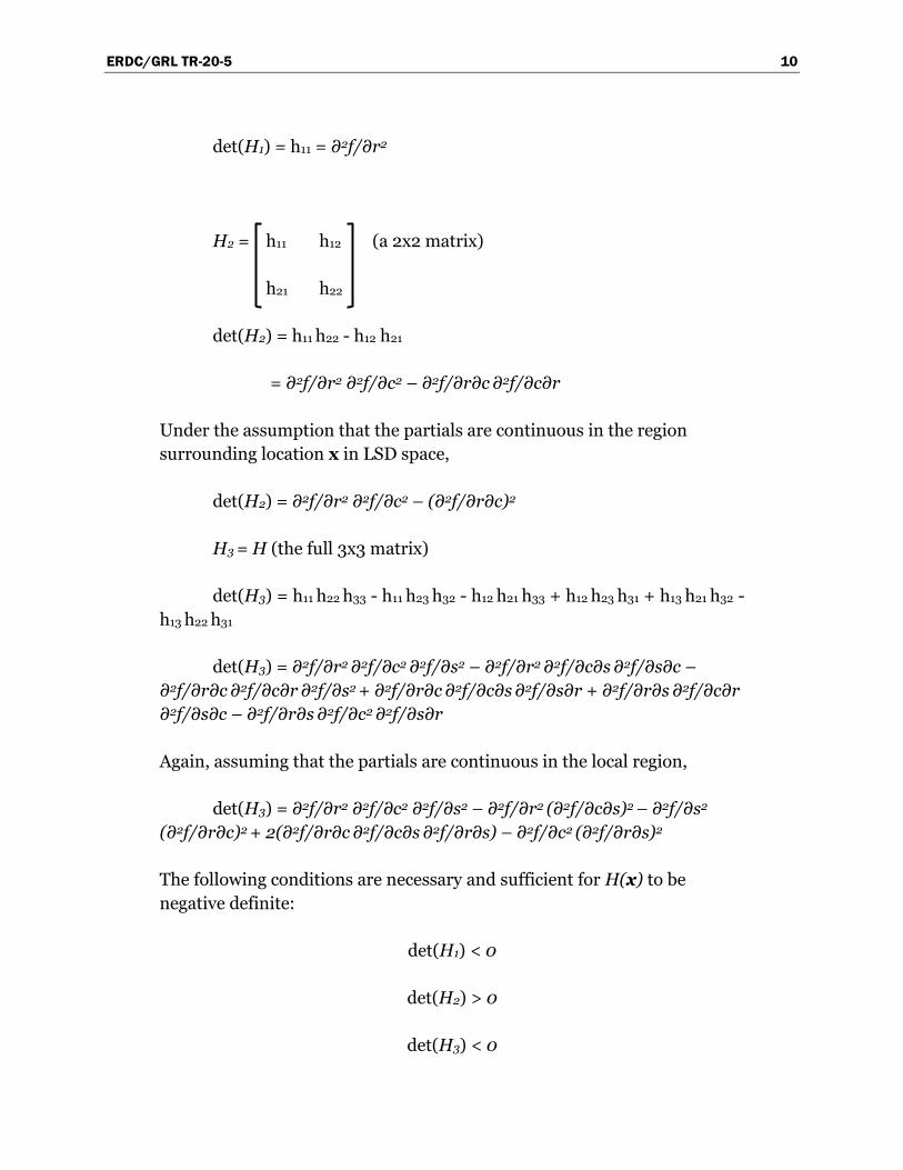
det(H1) = h11 = ∂2f/∂r2

H2 = h11 h12 (a 2x2 matrix)

h21 h22

det(H2) = h11 h22 - h12 h21

= ∂2f/∂r2 ∂2f/∂c2 – ∂2f/∂r∂c ∂2f/∂c∂r

Under the assumption that the partials are continuous in the region

surrounding location x in LSD space,

det(H2) = ∂2f/∂r2 ∂2f/∂c2 – (∂2f/∂r∂c)2

H3 = H (the full 3x3 matrix)

det(H3) = h11 h22 h33 - h11 h23 h32 - h12 h21 h33 + h12 h23 h31 + h13 h21 h32 -

h13 h22 h31

det(H3) = ∂2f/∂r2 ∂2f/∂c2 ∂2f/∂s2 – ∂2f/∂r2 ∂2f/∂c∂s ∂2f/∂s∂c –

∂2f/∂r∂c ∂2f/∂c∂r ∂2f/∂s2 + ∂2f/∂r∂c ∂2f/∂c∂s ∂2f/∂s∂r + ∂2f/∂r∂s ∂2f/∂c∂r

∂2f/∂s∂c – ∂2f/∂r∂s ∂2f/∂c2 ∂2f/∂s∂r

Again, assuming that the partials are continuous in the local region,

det(H3) = ∂2f/∂r2 ∂2f/∂c2 ∂2f/∂s2 – ∂2f/∂r2 (∂2f/∂c∂s)2 – ∂2f/∂s2

(∂2f/∂r∂c)2 + 2(∂2f/∂r∂c ∂2f/∂c∂s ∂2f/∂r∂s) – ∂2f/∂c2 (∂2f/∂r∂s)2

The following conditions are necessary and sufficient for H(x) to be

negative definite:

det(H1) < 0

det(H2) > 0

det(H3) < 0

ERDC/GRL TR-20-5 11

This test is applied to every location vector x in LSD space, ultimately

transforming LSD space into a “local maximum” space. x is a local

maximum of f(r,c,s) wherever H(x) is negative definite. The output from

these operations is, in theory, the set of optimal sample sizes associated

with the subset of x vectors defined by the negative definiteness property

of H(x) across the image or spatial dataset as determined by the LSD

approach. These may be mapped to particular feature objects in the data

with relatively uniform spatial frequencies to determine the optimal

sample sizes generated by different features. If a single optimal sample

size for the full dataset is desired, a weighted mean may be taken of the full

set of derived sample sizes.

In this treatment, the mean of the set of sample sizes associated with the

set of LSD local maxima determined by the above procedure will be

weighted by the LSD value associated with each local maximum. Because

every location in the dataset’s LSD space is investigated for a possible local

maximum, this single average sample size will be implicitly weighted by

the area of individual feature objects that generate similar optimal sample

sizes due to a relatively uniform spatial frequency response in the data.

2.3.2 Peakedness and optimal sample size

This complete set of local maxima may not be of uniform quality in terms

of the robustness of each maximum found for LSD = f(r,c,s). That is, there

may be some very weak or “shallow” maxima that are barely included in

the set because they meet the requirements for negative definiteness near

the limits of precision for the floating point numbers used in the

calculations. These maxima may have spurious accuracies and may not

represent the spatial frequencies of the underlying image or spatial data

feature. It may be useful, therefore, to apply a threshold to exclude these

lower-quality maxima. The term “peakedness” will be used to describe the

strength or quality of the LSD local maximum.

The peakedness of each local maximum will be calculated using the

Laplacian of the function LSD = f(r,c,s) evaluated at each point

determined by the Hessian matrix calculations. From vector analysis, the

Laplacian is a term that means the “divergence of the gradient” of a scalar

function, and is itself a scalar quantity. For a local maximum of a

multivariate function, the Laplacian will be a negative number. The more

“peaked” the local maximum, the more negative the number. In this way,

the range of Laplacian values can be calculated for the initial full set of

ERDC/GRL TR-20-5 12

local maxima, and then a chosen threshold can be applied expressed as a

percentage of that range to include only those maxima with Laplacian

values more negative than the threshold. The full set of local maxima in

LSD space is equivalent to a threshold of zero.

For the purposes here, the scalar function is LSD = f(r,c,s). The Laplacian

at any point (r,c,s) is then given by

∇2 f = ∂2f/∂r2 + ∂2f/∂c2 + ∂2f/∂s2

Fortunately, these second-order partial derivatives were already estimated

numerically when calculating the Hessian matrix for each location in LSD

space, and comprise the principal diagonal of the matrix. They are now

available to calculate the Laplacian for the set of local maxima determined

by the Hessian matrix analysis. To do this, the trace (the sum of elements

of the principal diagonal) is found of each Hessian matrix tr(Hrcs) in LSD

space. The full range of Laplacian values, or peakedness, in LSD space can

then be found.

The final step in this process is the calculation of optimal sample size.

Using peakedness, the effect of different thresholds on the process of

finding an optimal sample size for the whole image can be explored. The

optimal size is defined as the mean of the set of sample sizes associated

with the LSD space locations of the set of local maxima after applying a

chosen Laplacian threshold, if desired. This mean is weighted by the

number of local maxima and their associated LSD values at each sample

size. It is given by

𝑆𝑜𝑝𝑡 = ∑ 𝐿𝑆𝐷(𝑙𝑚𝑎𝑥𝑖,𝑗)𝑆𝑖

𝑛,𝑚

𝑖,𝑗=1

∑ 𝐿𝑆𝐷(𝑙𝑚𝑎𝑥𝑖,𝑗

𝑛,𝑚

𝑖.𝑗=1

⁄ )

where

Sopt = optimal sample size

i = resampled image number

n = total number of resampled images

m = total number of LSD local maxima in resampled image i

LSD(lmaxi,j) = for image i, the LSD value for each j of m local maxima with

peakedness above a given threshold

Si = sample size of image i

ERDC/GRL TR-20-5 13

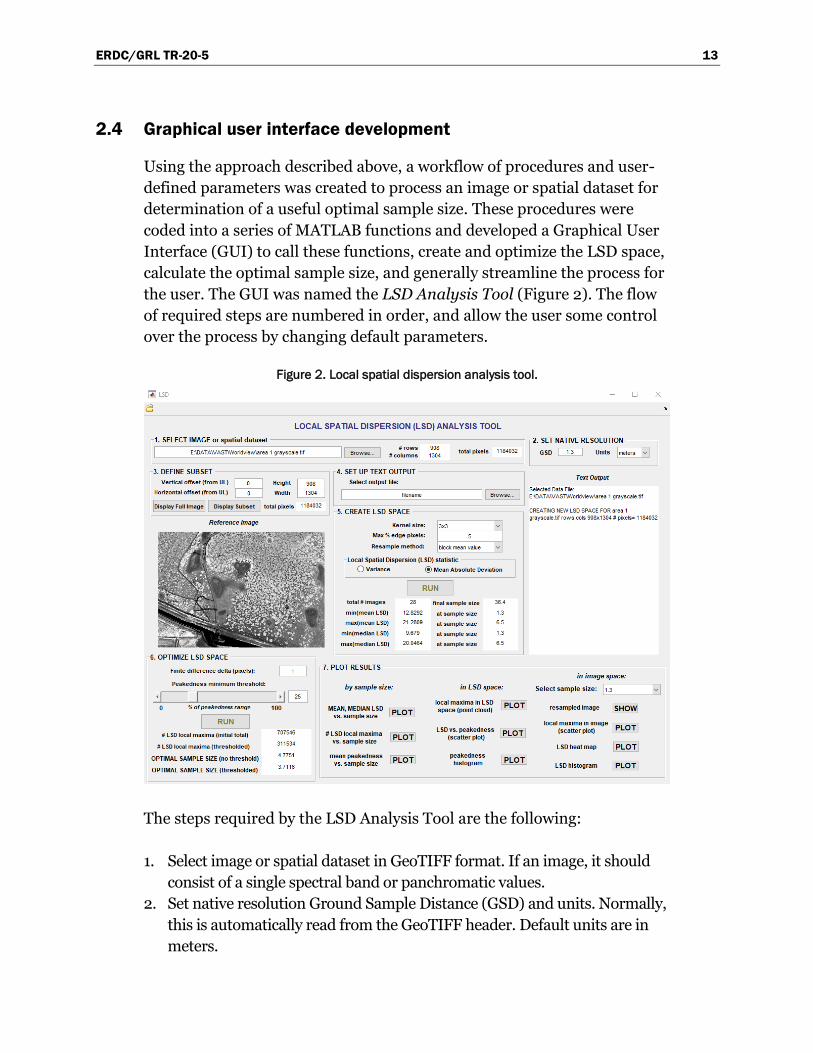
2.4 Graphical user interface development

Using the approach described above, a workflow of procedures and user-

defined parameters was created to process an image or spatial dataset for

determination of a useful optimal sample size. These procedures were

coded into a series of MATLAB functions and developed a Graphical User

Interface (GUI) to call these functions, create and optimize the LSD space,

calculate the optimal sample size, and generally streamline the process for

the user. The GUI was named the LSD Analysis Tool (Figure 2). The flow

of required steps are numbered in order, and allow the user some control

over the process by changing default parameters.

Figure 2. Local spatial dispersion analysis tool.

The steps required by the LSD Analysis Tool are the following:

1. Select image or spatial dataset in GeoTIFF format. If an image, it should

consist of a single spectral band or panchromatic values.

2. Set native resolution Ground Sample Distance (GSD) and units. Normally,

this is automatically read from the GeoTIFF header. Default units are in

meters.

ERDC/GRL TR-20-5 14

3. Define subset. The user can display and process a subset of the original

image by declaring the vertical and horizontal offsets from the upper left

corner of the image, and the height and width of the subset. Default values

are for the entire image.

4. Select output file to hold a text summary of processing output.

5. Create LSD space. LSD is calculated as a neighborhood function to find

residuals between each kernel element and the mean value of the kernel

throughout each resampled image. The user has control over the size of the

kernel (default is 3x3 pixels) as well as the choice of dispersion statistic:

LSV or MAD. As with LSV, MAD computes residuals, but takes their

absolute value rather than squaring them. The number of resampled

images created is controlled by the maximum percentage of edge pixels

(default 5%). The higher this number, the more images can be created.

There are three choices for the image resample method: pixel block mean

value (the default), bilinear interpolation, and bicubic interpolation. After

these parameters are chosen, the ‘RUN’ button is depressed to create the

LSD space from the sequence of resampled images.

6. Optimize LSD space. Here, the user can choose to set a minimum

peakedness threshold (default 25% of the peakedness range). The finite

difference delta (default 1) is the pixel interval used in the finite difference

equations needed for Hessian optimization. The optimization process

begins on depressing the ‘RUN’ button. The number of LSD local maxima

found is then shown, both with and without the peakedness threshold.

Finally, the relevant optimal sample sizes are displayed.

7. Plot results. The user can display the processed image at any sample size

and has nine plotting options to display the results of processing for the

chosen parameters. The various plotting options are grouped in relation to

sample size, LSD space, and image space. These plots show the behavior

and distribution of computed local maxima and LSD values, and may offer

clues to exploring other parameter options with repeated experimentation.

The available plots are:

a. Mean and median LSD vs. sample size

b. Number of LSD local maxima vs. sample size (semilog plot)

c. Mean peakedness vs. sample size

d. Point cloud distribution of local maxima in LSD space

e. Scatter plot of all LSD space values vs. peakedness

f. Histogram of peakedness for all local maxima

g. Scatter plot of local maxima for a chosen sample size

h. Heat map of LSD values for a chosen sample size

i. Histogram of LSD values for a chosen sample size

ERDC/GRL TR-20-5 15

The LSD Analysis Tool is designed to allow the user to quickly assess

spatial datasets of wide-ranging spatial structure for optimal sample size

by applying this novel approach of weighted means of distributed

dispersion local maxima. Trial-and-error runs can be performed easily,

using different combinations of user-controlled parameters. For example,

by changing the peakedness threshold and plotting results, the user can

explore the distribution of local maxima in relation to known features

across the image space for a chosen sample size, as well as in the

orthogonal sample size dimension.

ERDC/GRL TR-20-5 16

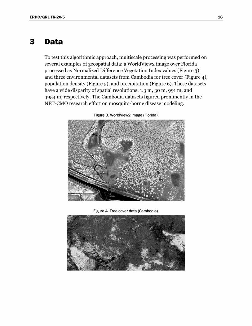
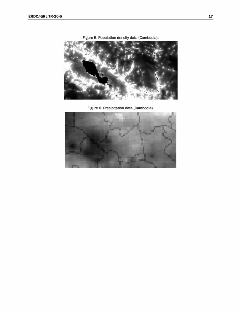
3 Data

To test this algorithmic approach, multiscale processing was performed on

several examples of geospatial data: a WorldView2 image over Florida

processed as Normalized Difference Vegetation Index values (Figure 3)

and three environmental datasets from Cambodia for tree cover (Figure 4),

population density (Figure 5), and precipitation (Figure 6). These datasets

have a wide disparity of spatial resolutions: 1.3 m, 30 m, 991 m, and

4954 m, respectively. The Cambodia datasets figured prominently in the

NET-CMO research effort on mosquito-borne disease modeling.

Figure 3. WorldView2 image (Florida).

Figure 4. Tree cover data (Cambodia).

ERDC/GRL TR-20-5 17

Figure 5. Population density data (Cambodia).

Figure 6. Precipitation data (Cambodia).

ERDC/GRL TR-20-5 18

4 Results

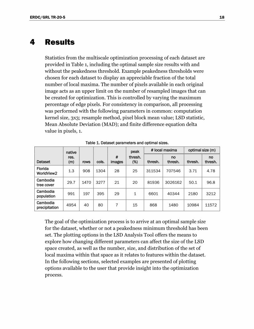
Statistics from the multiscale optimization processing of each dataset are

provided in Table 1, including the optimal sample size results with and

without the peakedness threshold. Example peakedness thresholds were

chosen for each dataset to display an appreciable fraction of the total

number of local maxima. The number of pixels available in each original

image acts as an upper limit on the number of resampled images that can

be created for optimization. This is controlled by varying the maximum

percentage of edge pixels. For consistency in comparison, all processing

was performed with the following parameters in common: computation

kernel size, 3x3; resample method, pixel block mean value; LSD statistic,

Mean Absolute Deviation (MAD); and finite difference equation delta

value in pixels, 1.

Table 1. Dataset parameters and optimal sizes.

Dataset

native

res.

(m) rows cols.

#

images

peak

thresh.

(%)

# local maxima optimal size (m)

thresh.

no

thresh. thresh.

no

thresh.

Florida

WorldView2 1.3 908 1304 28 25 311534 707546 3.71 4.78

Cambodia

tree cover 29.7 1470 3277 21 20 81936 3026162 50.1 96.8

Cambodia

population 991 197 395 29 1 6601 40344 2180 3212

Cambodia

precipitation 4954 40 80 7 15 868 1480 10984 11572

The goal of the optimization process is to arrive at an optimal sample size

for the dataset, whether or not a peakedness minimum threshold has been

set. The plotting options in the LSD Analysis Tool offers the means to

explore how changing different parameters can affect the size of the LSD

space created, as well as the number, size, and distribution of the set of

local maxima within that space as it relates to features within the dataset.

In the following sections, selected examples are presented of plotting

options available to the user that provide insight into the optimization

process.

ERDC/GRL TR-20-5 19

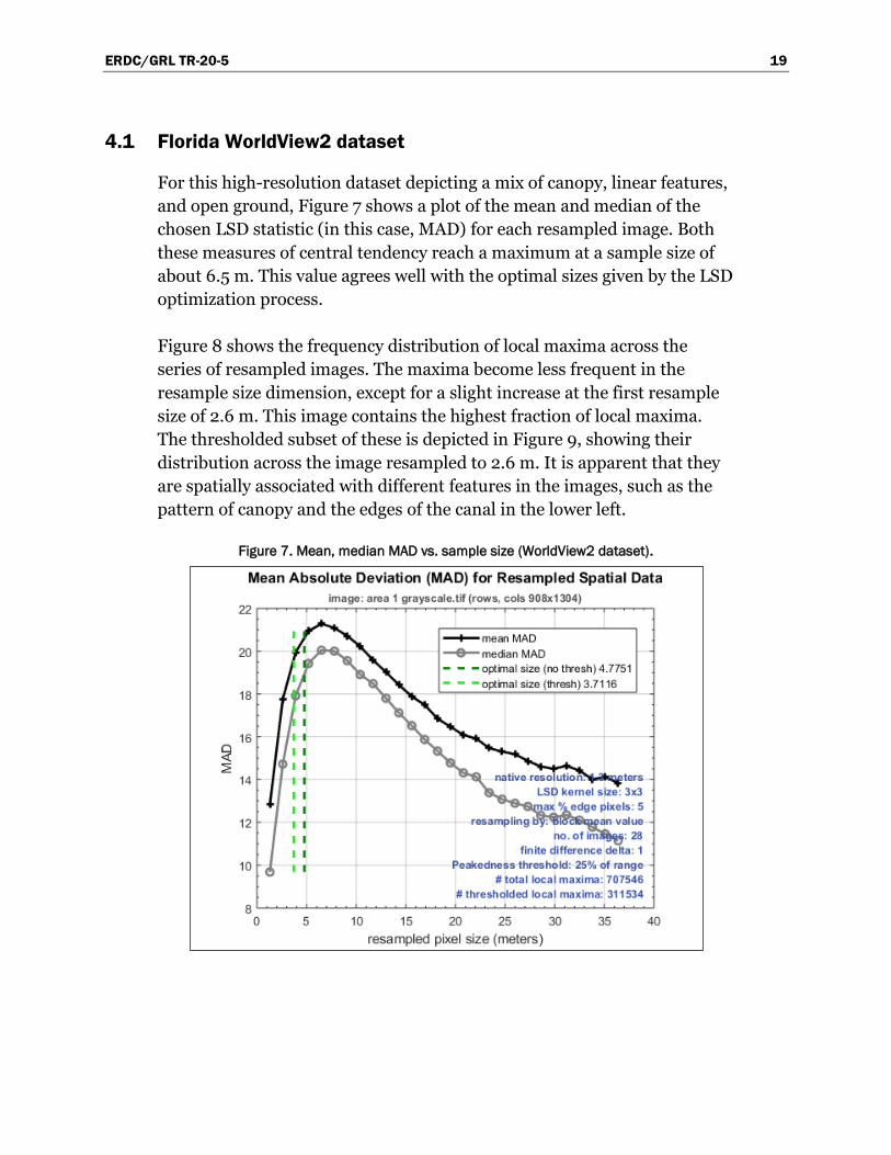
4.1 Florida WorldView2 dataset

For this high-resolution dataset depicting a mix of canopy, linear features,

and open ground, Figure 7 shows a plot of the mean and median of the

chosen LSD statistic (in this case, MAD) for each resampled image. Both

these measures of central tendency reach a maximum at a sample size of

about 6.5 m. This value agrees well with the optimal sizes given by the LSD

optimization process.

Figure 8 shows the frequency distribution of local maxima across the

series of resampled images. The maxima become less frequent in the

resample size dimension, except for a slight increase at the first resample

size of 2.6 m. This image contains the highest fraction of local maxima.

The thresholded subset of these is depicted in Figure 9, showing their

distribution across the image resampled to 2.6 m. It is apparent that they

are spatially associated with different features in the images, such as the

pattern of canopy and the edges of the canal in the lower left.

Figure 7. Mean, median MAD vs. sample size (WorldView2 dataset).

ERDC/GRL TR-20-5 20

Figure 8. Number of Local maxima vs. sample size (WorldView2 dataset).

Figure 9. Local maxima distribution at sample size 2.6 m (WorldView2 dataset).

The full distribution of thresholded local maxima in LSD space is shown as

a point cloud in perspective view in Figure 10. Note the influence of the

image’s linear features in the vertical distribution of local maxima.

ERDC/GRL TR-20-5 21

Figure 10. Local maxima distribution in LSD space (WorldView2 dataset).

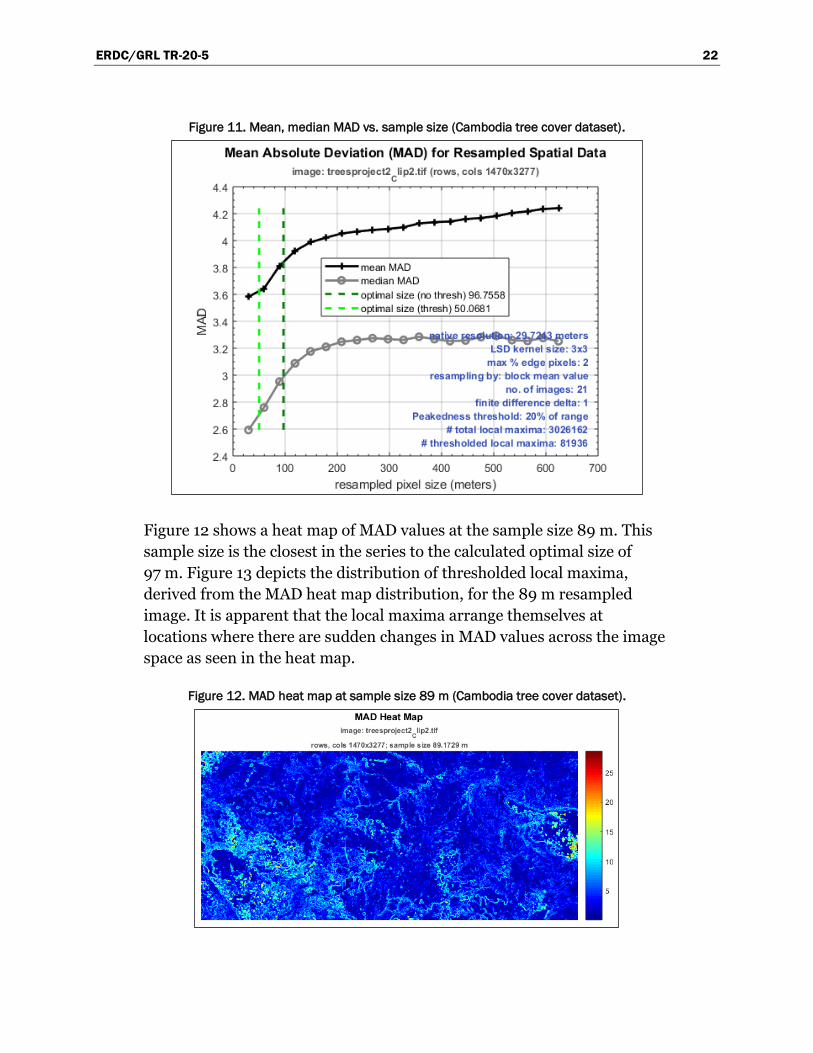
4.2 Cambodia tree cover dataset

Figure 11 shows a plot of the MAD mean and median for each resampled

image. In this case, their plots do not reach a local maximum against

resample size, so they do not give an indication of an optimal size. In spite

of this, the LSD optimization method provides optimal sizes of 97 m

(unthresholded) and 50 m (thresholded) for a native resolution of 30 m.

ERDC/GRL TR-20-5 22

Figure 11. Mean, median MAD vs. sample size (Cambodia tree cover dataset).

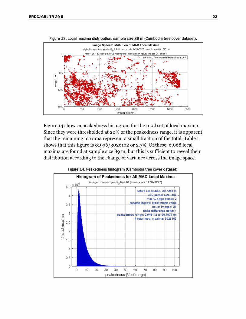
Figure 12 shows a heat map of MAD values at the sample size 89 m. This

sample size is the closest in the series to the calculated optimal size of

97 m. Figure 13 depicts the distribution of thresholded local maxima,

derived from the MAD heat map distribution, for the 89 m resampled

image. It is apparent that the local maxima arrange themselves at

locations where there are sudden changes in MAD values across the image

space as seen in the heat map.

Figure 12. MAD heat map at sample size 89 m (Cambodia tree cover dataset).

ERDC/GRL TR-20-5 23

Figure 13. Local maxima distribution, sample size 89 m (Cambodia tree cover dataset).

Figure 14 shows a peakedness histogram for the total set of local maxima.

Since they were thresholded at 20% of the peakedness range, it is apparent

that the remaining maxima represent a small fraction of the total. Table 1

shows that this figure is 81936/3026162 or 2.7%. Of these, 6,068 local

maxima are found at sample size 89 m, but this is sufficient to reveal their

distribution according to the change of variance across the image space.

Figure 14. Peakedness histogram (Cambodia tree cover dataset).

ERDC/GRL TR-20-5 24

4.3 Cambodia population density dataset

This dataset contains a large body of water within which there are no

values. Higher population densities surround the lake and line the

watercourses that empty into it. As reported in Table 1, the calculated

thresholded and unthresholded optimal sample sizes are 2,180 and

3,212 m, respectively, given the native spatial resolution of 991 m.

Figure 15 shows an upward trend in the MAD mean and median plots for

the lower sample sizes in the series of 29 images, along with the computed

optimal sizes of 2,180 m and 3,212 m for thresholded and unthresholded

peakedness, respectively.

Figure 15. Mean, median MAD vs. sample size (Cambodia population dataset).

Figure 16 shows the MAD heat map for the resample size 2,972 m, the size

closest to the unthresholded optimal value. The full point cloud

distribution of thresholded local maxima in LSD space derived from the

MAD values is shown in Figure 17. However, in this view, we are looking

straight down along the sample size axis at the local maxima found in the

entire resampled image series.

ERDC/GRL TR-20-5 25

Figure 16. MAD heat map, sample size 2,972 m (Cambodia population dataset).

Figure 17. Local maxima distribution in LSD Space, Vertical View (Cambodia population

dataset).

Figure 18 shows a scatter plot of MAD values for all local maxima in LSD

space, plotted against their peakedness values. This plot gives the user a

sense of how the maxima are distributed across the peakedness range as

well as the range of dispersion from which they were derived. Figure 19 is a

plot of mean peakedness for each image in the resample series, showing

that it is highest at the original spatial resolution and then drops down to a

relatively constant value as sample size increases.

ERDC/GRL TR-20-5 26

Figure 18. Scatter plot of MAD vs. peakedness (Cambodia population dataset).

Figure 19. Mean peakedness for resampled images (Cambodia population dataset).

ERDC/GRL TR-20-5 27

4.4 Cambodia precipitation dataset

For this dataset with the largest native resolution of 4,954 m, the plot of the

MAD mean and median for each resampled image is shown (Figure 20). In

this case, their plots not only do not reach a local maximum against

resample size, but also continue an upward trend through the resample size

series. Yet, the LSD optimization approach still provides reasonable optimal

sizes of 11,572 m (unthresholded) and 10,984 m (thresholded).

Figure 20. Mean, median MAD vs. sample size (Cambodia precipitation dataset).

The sample size in the resampled image series closest to the calculated

optimal sizes is 9,909 m. Figure 21 is a histogram of the frequency of MAD

values in the image with that spatial resolution, showing a maximum at a

MAD value of about 10-12 m. A MAD heat map is provided for sample size

9,909 m in Figure 22. Here, one can see that the higher dispersion values

are associated with transition zones with higher spatial frequencies in the

original image. Finally, Figure 23 shows a perspective view of the point

cloud of thresholded local maxima throughout LSD space. Their

distribution appears more homogeneous at higher levels in the space.

ERDC/GRL TR-20-5 28

Figure 21. MAD value frequency histogram, sample size 9,908 m (Cambodia

precipitation dataset).

Figure 22. MAD heat map, sample size 9,908 m (Cambodia precipitation dataset).

ERDC/GRL TR-20-5 29

Figure 23. Local maxima distribution in LSD space (Cambodia precipitation dataset).

ERDC/GRL TR-20-5 30

5 Discussion

In order to test this particular optimization approach, the algorithms that

implement it, and the LSD Analysis Tool, a small suite of images were

selected that represented a wide range of native resolutions, feature data

types, and spatial frequency regimes. Optimal sample sizes were

successfully calculated in all cases that scaled well with initial resolutions as

shown in Table 1. To maintain a degree of consistency, the following

processing parameters were kept constant for all four datasets: computation

kernel size, resample method, LSD statistic, and the delta interval for the

finite difference equations. At the time of writing, it is not known how

modification of these processing parameters would affect results in terms of

computed optimal sample sizes or local maxima distributions.

The results showed that optimal sizes for thresholded peakedness were

always slightly less than those that were unthresholded. The separation

depends on the choice of threshold. This suggests that local maxima with

lower values of peakedness are more concentrated near the top of LSD

space, increasing the representation of smaller resample sizes in the

weighting process. In fact, it was found that the mean peakedness for each

image in LSD space was highest for the original resolution of each dataset

in the study. This result, as depicted in Figure 19, is typical.

In this methodology, optimal sample size results are driven by the number

and distribution of LSD local maxima as well as the LSD values associated

with each local maximum. If a peakedness threshold is chosen, the set of

local maxima is first winnowed by a minimum peakedness value. Whatever

final set of maxima is used for optimization, they end up arranged in LSD

space according to feature locations at each sample size and define the

patterns of changing spatial frequencies therein (Figures 9, 13, and 17).

The setting of a peakedness threshold can be a useful tool for exploring the

distribution and peakedness of the local maxima set in LSD space by

examination of various plotting options in the LSD Analysis Tool. A

threshold is required if the retention of only high-value LSD optima for

optimal sample size calculations is indicated. However, a general strategy

has not been identified for choosing a threshold and, absent a supporting

rationale for its use, we recommend selecting the unthresholded optimal

size as a default procedure.

ERDC/GRL TR-20-5 31

Dispersion heat maps may be useful in depicting the pattern of subtle

changes of spatial frequency inherent in the data (Figures 12, 16, and 22).

These maps may show structure not easily gleaned from a casual

examination of the original spatial data. Figure 16 shows small

concentrations of population density within the general region of higher

dispersion values around the large lake as seen in Figure 5. This pattern is

reflected in the local maxima distribution map of Figure 17. The

distribution clearly associates with population density around the lake and

along several watercourses that empty into it.

Perspective view plots of the point cloud of local maxima in LSD space can

demonstrate how they are associated with features at various sample sizes

(Figures 10 and 23). This association may extend well into the upper

reaches of LSD space as vertical features (Figure 10), or appear to acquire

a more homogeneous distribution at some point above the lowest sample

sizes (Figure 23).

The WorldView2 dataset was the only one showing a distinct maximum (at

a sample size of 6-7 m) of the mean and median for the LSD function of

sample size (Figure 7). Tree cover dominates this image. As suggested by

previous research, this LSD maximum may reflect the average size of

individual canopies visible in the image, and may be most sensitive to the

image’s predominant spatial variation. Earlier researchers have considered

the LSD maximum, where it exists, in different ways in light of their image

analysis objectives. These results indicate an optimal sample size of 4.8 m,

slightly less than that indicated by the LSD function maximum.

Results from the WorldView2 dataset suggest that this optimization

approach is in general agreement with previous work on the interpretation

of the LSD function maximum for a particular sample size. As shown in

Figures 7 and 8, it is found that a somewhat smaller sample size than that

indicated by the LSD function maximum is optimal, and may be driven by

the preponderance of local LSD maxima at lower sample sizes.

Results show that this optimization technique for a multidimensional LSD

function successfully processes the inherent dispersion of image data with

heterogeneous spatial structure. Most importantly, it provides an optimal

sample size whether or not a maximum for the mean LSD function of

sample size exists (Figures 11, 15, and 20).

ERDC/GRL TR-20-5 32

6 Summary and Conclusions

The spatial characteristics of continuously varying phenomena on the

Earth’s surface directly inform remotely sensed data or other types of

environmental information collected in a geospatial context. The spatial

domain or structure of this data can be used to optimize its interpretation

or extraction of spatial information. Effective mapping or modeling of

spatially dependent information requires capturing the spatial variation

patterns of features of interest. A key consideration in image analysis is the

relationship between spatial resolution and the spatial frequency structure

of features found in the image data.

In this work, this relationship was examined through a multiscale

modeling approach to determine an optimal sample size for raster images

containing remotely sensed or other environmental data with variable

spatial structure. Resampling an image dataset in this way can increase the

efficiency of image processing functions, such as feature segmentation or

of geospatial models, such as that employed in the NET-CMO project at

ERDC-GRL. Four image datasets were analyzed with disparate native

resolutions collected over Florida and Cambodia. These datasets depict a

variety of environmental feature data with heterogeneous spatial

structure. In each case, a multidimensional dispersion space was created

from which sets of local maxima were extracted. These local maxima were

used in a weighted mean formulation to compute optimal sample sizes

that did not depend on the single-variable functional relationship between

mean dispersion and resample size. This approach captures the locality of

variance in heterogeneous spatial datasets rather than relying on an

overall mean dispersion value for each resampled image.

A useful tool and user interface was created, the LSD Analysis Tool, to

exercise our algorithmic approach and allow a user to process a dataset

while in control of particular processing parameters. Various plotting

options display relationships among LSD values, local LSD maxima,

maxima peakedness, and LSD space locations. These output features and

level of user control provide for repeated experimentation and a better

understanding of the spatial structure of the data.

The authors believe that this multiscale modeling approach to optimizing

sample size is an effective and robust method as applied to geospatial data.

ERDC/GRL TR-20-5 33

References

Atkinson, P. M., and P. J. Curran. 1995. Defining an optimal size of support for remote sensing investigations. IEEE Transactions on Geoscience and Remote Sensing 33:768-776.

Chapra, S. C., and R. P. Canale. 2002. Numerical methods for engineers: with software and programming applications. Fourth ed., p. 355. New York: McGraw-Hill.

Costanza, R., and T. Maxwell. 1994. Resolution and predictability: An approach to the scaling problem. Landscape Ecology 9(1):47-57.

Curran, P. J. 2001. Remote sensing: Using the spatial domain. Environmental and Ecological Statistics 8:331-344.

Curran, P. J., P. M. Atkinson, G. M. Foody, and E. J. Milton. 2000. Linking remote sensing, land cover, and disease. Advances in Parasitology 47:37-81.

Goodchild, M. F. 2011. Scale in GIS: An overview. Geomorphology 130:5-9.

Marceau, D. J., D. J. Gratton, R. A. Fournier, and J. P. Fortin. 1994. Remote sensing and the measurement of geographical entities in a forested environment 2. The optimal spatial resolution. Remote Sensing of Environment 49:105-117.

McCloy, K. R., and P .K. Bøcher. 2007. Optimizing image resolution to maximize the accuracy of hard classification. Photogrammetric Engineering and Remote Sensing 73(8):893-903.

Rahman, A. F., J. A. Gamon, D. A. Sims, and M. Schmidts. 2003. Optimum pixel size for hyperspectral studies of ecosystem function in southern California chaparral and grassland. Remote Sensing of Environment 84:192-207.

Richards, J. A., and X. Jia. 1999. Remote sensing digital image analysis: an introduction. 3rd ed., pp. 162-164. Berlin Heidelberg: Springer-Verlag.

Woodcock, C. E., and A. H. Strahler. 1987. The factor of scale in remote sensing. Remote Sensing of Environment 21:311-322.

ERDC/GRL TR-20-5 34

Acronyms and Abbreviations

Acronym Meaning

ERDC Engineer Research and Development Center

GRL Geospatial Research Laboratory

GSD Ground Sample Distance

GUI Graphical User Interface

LSD Local Spatial Dispersion

LSV Local Spatial Variance

MAD Mean Absolute Deviation

NET-CMO New and Enhanced Tools for Civil-Military Operations

USACE U.S. Army Corps of Engineers

REPORT DOCUMENTATION PAGE Form Approved OMB No. 0704-0188

Public reporting burden for this collection of information is estimated to average 1 hour per response, including the time for reviewing instructions, searching existing data sources, gathering and maintaining the data needed, and completing and reviewing this collection of information. Send comments regarding this burden estimate or any other aspect of this collection of information, including suggestions for reducing this burden to Department of Defense, Washington Headquarters Services, Directorate for Information Operations and Reports (0704-0188), 1215 Jefferson Davis Highway, Suite 1204, Arlington, VA 22202-4302. Respondents should be aware that notwithstanding any other provision of law, no person shall be subject to any penalty for failing to comply with a collection of information if it does not display a currently valid OMB control number. PLEASE DO NOT RETURN YOUR FORM TO THE ABOVE ADDRESS.

1. REPORT DATE (DD-MM-YYYY)

February 2020

2. REPORT TYPE

Final report 3. DATES COVERED (From - To)

4. TITLE AND SUBTITLE

Local Spatial Dispersion for Multiscale Modeling of Geospatial Data: Exploring Dispersion

Measures to Determine Optimal Raster Data Sample Sizes

5a. CONTRACT NUMBER

5b. GRANT NUMBER

5c. PROGRAM ELEMENT NUMBER

62784

6. AUTHOR(S)

S. Bruce Blundell and Nicole M. Wayant

5d. PROJECT NUMBER

855

5e. TASK NUMBER

22

5f. WORK UNIT NUMBER

7. PERFORMING ORGANIZATION NAME(S) AND ADDRESS(ES) 8. PERFORMING ORGANIZATION REPORT NUMBER

Geospatial Research Laboratory

U.S. Army Engineer Research and Development Center

7701 Telegraph Road

Alexandria, VA 22315-3864

ERDC/GRL TR-20-5

9. SPONSORING / MONITORING AGENCY NAME(S) AND ADDRESS(ES) 10. SPONSOR/MONITOR’S ACRONYM(S)

Headquarters, U.S. Army Corps of Engineers

Washington, DC 20314-1000

11. SPONSOR/MONITOR’S REPORT NUMBER(S)

12. DISTRIBUTION / AVAILABILITY STATEMENT

Approved for public release; distribution unlimited.

13. SUPPLEMENTARY NOTES

14. ABSTRACT

Scale, or spatial resolution, plays a key role in interpreting the spatial structure of remote sensing imagery or other geospatially

dependent data. These data are provided at various spatial scales. Determination of an optimal sample or pixel size can benefit

geospatial models and environmental algorithms for information extraction that require multiple datasets at different resolutions. To

address this, an analysis was conducted of multiple scale factors of spatial resolution to determine an optimal sample size for a

geospatial dataset. Under the NET-CMO project at ERDC-GRL, a new approach was developed and implemented for determining

optimal pixel sizes for images with disparate and heterogeneous spatial structure. The application of local spatial dispersion was

investigated as a three-dimensional function to be optimized in a resampled image space. Images were resampled to progressively

coarser spatial resolutions and stacked to create an image space within which pixel-level maxima of dispersion was mapped. A weighted

mean of dispersion and sample sizes associated with the set of local maxima was calculated to determine a single optimal sample size

for an image or dataset. This size best represents the spatial structure present in the data and is optimal for further geospatial modeling.

15. SUBJECT TERMS

Remote sensing

Geographic data

Geospatial data

Remote sensing images

Image processing

Optimization

Geographic information systems

Multiscale modeling

Algorithms

16. SECURITY CLASSIFICATION OF: 17. LIMITATION OF ABSTRACT

18. NUMBER OF PAGES

19a. NAME OF RESPONSIBLE PERSON

a. REPORT

UNCLASSIFIED

b. ABSTRACT

UNCLASSIFIED

c. THIS PAGE

UNCLASSIFIED SAR 42

19b. TELEPHONE NUMBER (include

area code)

Standard Form 298 (Rev. 8-98) Prescribed by ANSI Std. 239.18