Geometric Methods in Machine Learning

Arvind AgwaralDepartment of Computer Science

University of MarylandCollege Park Maryland, USA 20740

arvinda@cs.umd.edu

Abstract

The standard goal of machine learning to take a finite set of data and induce a model using that data that is ableto generalize beyond that finite set. In particular, a learning problem finds an appropriate statistical model from amodel space based on the training data from a data space. For many such problems, these spaces carry geometricstructures that can be exploited using geometric methods, or the problems themselves can be formulated in away that naturally appeals to geometry-based methods. In such cases, studying these geometric structures andthen using appropriate geometry-driven methods not only gives insight into existing algorithms, but also helpsbuild new and better algorithms. In my research, I apply geometric methods to a variety of learning problems, andprovide strong theoretical and empirical evidence in favor of using them.

The first part of my proposal is devoted to the study of the geometry of the space of probabilistic models associatedwith the statistical process that generated the data. This study – based on the theory well grounded in informationgeometry – allows me to reason about the appropriateness of conjugate priors from a geometric perspective, andhence gain insight into the large number of existing models that rely on these priors. Furthermore, I use this studyto build a family of kernels called generative kernels that can be used as off-the-shelf tool in any kernel learningmethod such as support vector machines. Preliminary experiments of generative kernels based on simple statisticalprocess show promising results, and in the future I propose to extend this work for more complex statisticalprocesses.

In the second part of the proposal, I apply geometric methods to the data space; in particular, I use existing toolsfrom computation geometry to build a unified framework for solving a well known problem multidimensionalscaling (MDS). This geometry-inspired framework results in algorithms which can solve different variants of MDSbetter than the previous state-of-the-art methods, and which have many other attractive properties: they aresimple, intuitive, easily parallelizable, scalable, and can handle missing data. Preliminary experiments showthe effectiveness of this framework for many variants of MDS. In future work, I plan to extend it for large scalestreaming data sets, and show its effectiveness by applying it to text documents.

Contents

1 Introduction 3

1.1 Goals of the proposed thesis . . . . . . . . . . . . . . . . . . . . . . . . . . . . . . . . . . . . . . . . . . . . 4

1.2 Proposal Outline . . . . . . . . . . . . . . . . . . . . . . . . . . . . . . . . . . . . . . . . . . . . . . . . . . . . 5

I Geoemetry in Models 6

2 Exponential Family and their Properties 7

2.1 Legendre Duality . . . . . . . . . . . . . . . . . . . . . . . . . . . . . . . . . . . . . . . . . . . . . . . . . . . 7

2.2 Bregman Divergence . . . . . . . . . . . . . . . . . . . . . . . . . . . . . . . . . . . . . . . . . . . . . . . . . 7

2.3 Exponential Family . . . . . . . . . . . . . . . . . . . . . . . . . . . . . . . . . . . . . . . . . . . . . . . . . . 8

3 A Geometric View of Conjugate Priors 10

3.1 Motivation . . . . . . . . . . . . . . . . . . . . . . . . . . . . . . . . . . . . . . . . . . . . . . . . . . . . . . . 10

3.2 Likelihood, Prior and Geometry . . . . . . . . . . . . . . . . . . . . . . . . . . . . . . . . . . . . . . . . . . 11

3.2.1 Likelihood in the form of Bregman Divergence . . . . . . . . . . . . . . . . . . . . . . . . . . . . 12

3.2.2 Conjugate Prior in the form of Bregman Divergence . . . . . . . . . . . . . . . . . . . . . . . . . 13

3.2.3 Geometric Interpretation of Conjugate Prior . . . . . . . . . . . . . . . . . . . . . . . . . . . . . . 14

3.2.4 Geometric Interpretation of Non-conjugate Prior . . . . . . . . . . . . . . . . . . . . . . . . . . . 15

3.3 Hybrid model . . . . . . . . . . . . . . . . . . . . . . . . . . . . . . . . . . . . . . . . . . . . . . . . . . . . . 15

3.3.1 Generalized Hybrid Model . . . . . . . . . . . . . . . . . . . . . . . . . . . . . . . . . . . . . . . . . 17

3.3.2 Geometry of the Hybrid Model . . . . . . . . . . . . . . . . . . . . . . . . . . . . . . . . . . . . . . 17

3.3.3 Prior Selection . . . . . . . . . . . . . . . . . . . . . . . . . . . . . . . . . . . . . . . . . . . . . . . . 18

3.4 Related Work and Conclusion . . . . . . . . . . . . . . . . . . . . . . . . . . . . . . . . . . . . . . . . . . . . 19

4 Generative Kernels 20

4.1 Background: Statistical Manifolds and Dualistic Structure . . . . . . . . . . . . . . . . . . . . . . . . . . 21

4.2 Generative Model to Metric . . . . . . . . . . . . . . . . . . . . . . . . . . . . . . . . . . . . . . . . . . . . . 22

4.3 Metric to Kernel . . . . . . . . . . . . . . . . . . . . . . . . . . . . . . . . . . . . . . . . . . . . . . . . . . . . 23

4.4 Preliminary Experiments . . . . . . . . . . . . . . . . . . . . . . . . . . . . . . . . . . . . . . . . . . . . . . . 24

1

4.5 Conclusion and Future Work . . . . . . . . . . . . . . . . . . . . . . . . . . . . . . . . . . . . . . . . . . . . 26

II Geoemetry in Data 27

5 Universal Multidimensional Scaling 28

5.1 Motivation . . . . . . . . . . . . . . . . . . . . . . . . . . . . . . . . . . . . . . . . . . . . . . . . . . . . . . . 28

5.2 Background and Existing Methods . . . . . . . . . . . . . . . . . . . . . . . . . . . . . . . . . . . . . . . . . 29

5.3 Definitions . . . . . . . . . . . . . . . . . . . . . . . . . . . . . . . . . . . . . . . . . . . . . . . . . . . . . . . 29

5.4 Algorithm . . . . . . . . . . . . . . . . . . . . . . . . . . . . . . . . . . . . . . . . . . . . . . . . . . . . . . . . 30

5.5 Experiments . . . . . . . . . . . . . . . . . . . . . . . . . . . . . . . . . . . . . . . . . . . . . . . . . . . . . . 32

6 Spherical Multidimensional Scaling 36

6.1 Algorithm . . . . . . . . . . . . . . . . . . . . . . . . . . . . . . . . . . . . . . . . . . . . . . . . . . . . . . . . 36

6.2 Experiments . . . . . . . . . . . . . . . . . . . . . . . . . . . . . . . . . . . . . . . . . . . . . . . . . . . . . . 37

6.3 Future Work: Application to Text Classification . . . . . . . . . . . . . . . . . . . . . . . . . . . . . . . . . 38

7 Large Scale Incremental Multidimensional Scaling 39

7.1 Existing Work . . . . . . . . . . . . . . . . . . . . . . . . . . . . . . . . . . . . . . . . . . . . . . . . . . . . . 39

7.2 Problem Definition . . . . . . . . . . . . . . . . . . . . . . . . . . . . . . . . . . . . . . . . . . . . . . . . . . 40

7.3 Batch Algorithm . . . . . . . . . . . . . . . . . . . . . . . . . . . . . . . . . . . . . . . . . . . . . . . . . . . . 41

7.4 Streaming Algorithm . . . . . . . . . . . . . . . . . . . . . . . . . . . . . . . . . . . . . . . . . . . . . . . . . 41

7.5 Future Work: Experimental Study . . . . . . . . . . . . . . . . . . . . . . . . . . . . . . . . . . . . . . . . . 42

8 Proposal at a glance 43

8.1 Timeline . . . . . . . . . . . . . . . . . . . . . . . . . . . . . . . . . . . . . . . . . . . . . . . . . . . . . . . . . 43

8.2 Contribution so far... . . . . . . . . . . . . . . . . . . . . . . . . . . . . . . . . . . . . . . . . . . . . . . . . . 43

8.3 Summary . . . . . . . . . . . . . . . . . . . . . . . . . . . . . . . . . . . . . . . . . . . . . . . . . . . . . . . . 44

Bibliography 45

2

Chapter 1

Introduction

Machine learning and geometry have mostly been two separate fields with little interdisciplinary researchbetween them. In the proposed research, my main goal is to show that the geometry-based methods can beused to gain insight into existing learning algorithms, and design new and better algorithms.

Here “geometric methods" refers to methods that treat data points as points (or vectors) in a geometric space andperform geometric operations on them. Examples of such operations include transformations, distance computation,the construction of geometric objects such as lines, triangles, or circles, and performing geometric operations onthese objects such as intersection computation. The strength of geometric methods lie in the fact that they help usvisualize the problem, thus providing additional insight into problems and existing algorithms, and often leadingto the development of new and better algorithms.

In machine learning, a learning problem takes a set of training points {x i}ni=1 as an input, which are assumed tocome from some space X, the data space. Given a such set of training points, the objective of a learning problem isto find a model defined by a set of parameters θ that explains the data well and generalizes to the future data.These parameters are selected from another space Θ, the model space. Under certain assumptions, these spacescarry inherent geometries to them which can be exploited using geometric methods. Since geometric methods relyexclusively on geometric operations, they have to respect the inherent geometry of the space associated with theproblem.

In this thesis, I apply geometric methods to a variety of problems, both in data space and in model space. I firststudy the geometric structure associated with the space of a problem, and then apply the appropriate geometrictools to solve it. I show that these methods are useful not only to gain insight into current learning algorithms,but also to design new algorithms that perform better than the state-of-the-art algorithms. These geometricmethods are based on the concepts based on information geometry [Spivak, 1999,Amari and Nagaoka, 2001],when analyzing the model space Θ; and concepts based on computational geometry [Preparata and Shamos, 1985]when analyzing the data space X.

This thesis is broadly divided into two parts. The first part is concerned with applying geometric methods to themodel space, while the second part concerns with applying these methods to the data space.

Geometric methods in model space: In the first part, I study the probabilistic models from a geometricperspective by treating the space of parameters Θ as geometric space and a parameter vector θ as a point inthat space. In machine learning, it is common to assume that the data is generated from an exponential familyparameterized by θ ∈ Θ, which has a geometric structure associated with it given by a natural metric (Fisherinformation metric) and an affine connection. In this work, I study this geometric structure, and use it to

3

reason about the appropriateness of conjugate priors, and hence gain insight into some existing models that relyon these priors. I also use this study to build a family of kernels called generative kernels. These kernels arebuilt considering the geometry associated with the generative model but are used in discriminative models, andtherefore they naturally combine the power of both discriminative and generative models. Preliminary experimentsdemonstrate this hybrid behavior i.e., performance of the discriminative/generative hybrid model is better than apure generative model, or a pure discriminative model alone.

Geometric methods in data space: In the second part of the thesis, I turn to the data space. Here the dataspace is given a similar treatment as the model space i.e., it is a geometric space, and points in this space areentities that are allowed to move, construct objects, and participate in arbitrary geometric operations. In machinelearning, it is a standard practice to treat data points as points (or vectors) in a geometric space, however it is invery few cases that these points actually participate in geometric operations leading to the development of thealgorithms. Often in machine learning, a learning problem is cast as an optimization problem, and the solution issought by directly solving the optimization problem using standard optimization methods. Although this approachto solving the learning problem is often successful, it is not the best solution for all problems. Many times, a bettersolution can be found by attacking the problem indirectly – by studying the geometry associated with the problem,and then using the appropriate geometric tools. For example, in my work, I solve a well known dimensionalityreduction problem called multidimensional scaling (MDS) by giving it a geometric treatment. Earlier methods solvethis problem by minimizing the cost function directly using the optimization methods, while I, on the other hand,use geometric operations (such as moving points in the space, adding two vectors, computing the vector-sum) tosolve it. By using these geometric operations, I am able to transform the original problem into a subproblem thatis well studied in computational geometry. This geometric treatment of the problem results in a framework thatnot only solves the original MDS problem in the Euclidean space more effectively than the state-of-the-art methods,but also generalizes to the other spaces i.e., spherical space; and has many desirable properties.

1.1 Goals of the proposed thesis

In this thesis, I claim that the geometric methods are useful not only to gain insight into existing algorithms, butalso to develop new algorithms. In order to support my claim, I take a variety of problems and show that thegeometric methods are indeed useful, by either getting a better understanding of the problem or by developingbetter algorithms to solve it. In this work, I specifically take three problems which cover a wide range of problemsin machine learning on many fronts. For example, these problems (or the proposed solutions) involve using thegeometry from both spaces, the data space and the model space; these problems cover different learning categoriese.g., supervised, semi-supervised, and unsupervised; they cover both kind of problems - analysis problems wheregeometric methods are used only to get a better understanding of the problem without resulting into any newalgorithms, and the problems where geometric methods are used not only to get a better understanding of theproblem, but also to develop new and better algorithms. The goals of this thesis are derived from these threeproblems, and are:

1. Understand the appropriateness of conjugate priors and their use in a generative/discriminative hybridmodel for classification.

2. Develop novel kernels that take into account the distribution associated with a generative model of the data.

3. Solve an unsupervised dimensionality reduction problem i.e. generalized multidimensional scaling.

4

1.2 Proposal Outline

In order to show the utility of geometric methods, I take a variety of problems, which as discussed above, cover awide range of learning problems – from supervised to semi-supervised to unsupervised. Under the semi-supervisedcategory, I use geometric methods to gain insight into hybrid models i.e., why it is appropriate to use the conjugateprior as a coupling prior to build these models(Chapter 3). In Chapter 4, I use geometric methods to build afamily of kernels called generative kernels that are then later used in supervised learning. Under the unsupervisedcategory, I use geometric methods to develop new algorithms for solving a dimensionality reduction problem, inparticular multidimensional scaling (MDS) (Chapters 5, 6, and 7).

Chapter 2 provides requisite background for the exponential family distributions. Additional background relevantto a specific section will appear in that section alone. The background provided in Chapter 2 is brief: for a morecomplete background, see [Amari and Nagaoka, 2001,Wainwright and Jordan, 2008].

A Geometric View of Conjugate Priors Chapter 3 is devoted to understanding how geometric methods canbe used to gain insight into existing algorithms by studying conjugate priors from a geometric perspective, andjustifying their use in hybrid generative/discriminative models. In Bayesian machine learning, conjugate priorsare popular, mostly due to mathematical and computational convenience. In this chapter, I study the geometryunderlying the exponential family distributions, and show that there are deeper reasons for choosing a conjugateprior. Specifically, I formulate the conjugate prior in the form of Bregman divergence and show that it is theinherent geometry of conjugate priors that makes them appropriate and intuitive. This geometric interpretationallows one to view the hyperparameters of conjugate priors as the effective sample points, and to reason about theuse of conjugate prior as a coupling prior in hybrid models.

Generative Kernels In Chapter 4, I use geometric methods to build generative kernels, a family of kernels thatcan be used as off-the-shelf tool in any kernel learning method such as support vector machines. These kernels arecalled generative kernels because they take into account the generative process of the data. My proposed methodconsiders the geometry of the space of statistical models associated with the distribution that generated the data,to build a set of efficient closed-form kernels best suited for that distribution. Although these kernels can be used inany kernel method, I use them in supervised text classification tasks, and observe improved empirical performance.

Universal Multi-Dimensional Scaling In the following chapters (5, 6, and 7) I apply geometric methods tothe data space, and show how these methods can be used to build powerful algorithms that can outperform thecurrent state-of-the-art algorithms. In Chapter 5, I show the utility of the geometric methods by building a unifiedalgorithmic framework for solving many known variants of MDS. The algorithms derived from my framework arebased on simple geometric operations as moving points in the space, computing intersections etc. In additionto the formal guarantees of convergence, these algorithms are accurate; in most cases, they converge to betterquality solutions than existing methods in comparable time. Moreover, they have a small memory footprint andscale effectively for large data sets. I expect that this framework will be useful for a number of MDS variants thathave not yet been studied. In Chapter 6, I use this unified MDS framework to solve a specific instance of MDS,known as spherical MDS, and propose to use in a text classification task assuming that the text documents lie on ahypersphere when represented as frequency vectors [Kass and Vos, 1997,Lebanon and Lafferty, 2004].

Large Scale Multidimensional Scaling In Chapter 7, I extend the unified MDS framework for large scalestreaming data. In particular, I propose an approximate version of the unified MDS framework which takesconstant time to process the new point in the stream, as opposed to the exact version that takes linear time. In thefuture, I plan to perform an empirical study of the proposed approximate algorithm.

5

Part I

Geoemetry in Models

6

Chapter 2

Exponential Family and their Properties

In chapters 3 and 4, I use the geometry underlying exponential family models to reason about conjugate priors, andbuild generative kernels. This chapter gives the required background, in particular, concepts related to Legendreduality, Bregman divergence, and exponential families.

2.1 Legendre Duality

Let M ⊆ Rd and Θ ⊆ Rd be two spaces and let F : M→ R+ and G : Θ→ R+ be two non-negative real valuedconvex functions. F and G are conjugate duals of each other if:

F(µ) := supθ∈Θ{⟨µ,θ ⟩ − G(θ)}, ∀µ ∈M (2.1)

and

G(θ) := supµ∈M{⟨θ ,µ⟩ − F(µ)}, ∀θ ∈Θ (2.2)

here ⟨a, b⟩ denotes the dot product of vectors a and b, R denotes the space of real numbers, Rd denotes thed-dimensional space of real numbers, and R+ denotes the space of non-negative real numbers. The spaces (Θand M) associated with these dual functions are called dual spaces; this relationship between them is know asLegendré duality or just the duality. There are standard notations to refer this duality i.e., G = F∗ and F = G∗.A particularly important connection between dual spaces is that: for each µ ∈M,∇F(µ) = θ ∈ Θ (denoted asµ∗ = θ)) and similarly, for each θ ∈ Θ,∇G(θ) = µ ∈M (or θ ∗ = µ)). For more details, refer to [Rockafellar,1996].

2.2 Bregman Divergence

I now give a brief overview of Bregman divergence (for more details see [Banerjee et al., 2005]). Let F : M→ R+be a continuously-differentiable real-valued and strictly convex function. The Bregman divergence (see Figure 2.1)associated with F for points µ1,µ2 ∈M is:

BF (µ1‖µ2) = F(µ1)− F(µ2)− ⟨∇F(µ2), (µ1 −µ2)⟩ (2.3)

7

µ2 µ1

F

BF (µ1‖µ2)

Figure 2.1: Geometric representation of Bregman divergence

If G is the conjugate dual of F then:

BF (µ1‖µ2) = BG(µ∗2‖µ

∗1) (2.4)

here µ∗1 and µ∗2 are the duals of µ1 and µ2 respectively. Note that the arguments are flipped in (2.4). Itis emphasized that Bregman divergence is not symmetric i.e., in general, BF (p‖q) 6= BF (q‖p), therefore it isimportant what directions these divergences are measured in.

2.3 Exponential Family

The exponential family is a set of distributions defined over a space X, whose probability density function for somex ∈ X can be expressed in the following form:

p(x;θ) = po(x)exp(⟨θ ,φ(x)⟩ − G(θ)) (2.5)

here φ(x) : X→ Rd is a vector potentials or sufficient statistics [Nielsen, 1978], po(x) is a function that dependson the base measure ν i.e., dν = p0(x) d x , and G(θ) is a normalization constant or log-partition function. Withthe potential functions φ(x) fixed, every θ induces a particular member p(x;θ) of the family. In the proposedresearch, I deal with exponential families that are regular and have the minimal representation. (For details on this,refer to [Wainwright and Jordan, 2008]).

The exponential family has a number of convenient properties and subsumes many common distributions. Itincludes the Gaussian, Binomial, Beta, Multinomial and Dirichlet distributions, hidden Markov models, Bayes nets,etc.. One important property of the exponential family is the existence of conjugate priors. Given any member ofthe exponential family as in (2.5), the conjugate prior is a distribution over its parameters with the following form:

p(θ |α,β) = m(α,β) exp(⟨θ ,α⟩ − βG(θ)) (2.6)

here α and β are hyperparameters of the conjugate prior. Importantly, the function G(·) is same between theexponential family member and its conjugate prior.

A second important property of exponential family member is that log-partition function G is a continuouslydifferentiable strictly convex function and defined over the convex set Θ := {θ ∈ Rd : G(θ )<∞}. These propertiesof log-partition function induce a Bregman divergence on the space Θ. Convexity of log-partition function Gensures that there exists a space M, dual to Θ and a dual function F defined over M. Here duality refers toLegendre duality. This convexity property also induces a Bregman divergence on both Θ and M.

8

θ1θn θ̂ML

µ1µn µML

Θ

M

G

F

Figure 2.2: Duality between mean parameters and canonical parameters. Notice the convex functions definedover both spaces. these functions are dual of each other and so are the spaces.

Another important property of the exponential family is the one-to-one mapping between the canonical parametersθ and the so-called “mean parameters” which we denote by µ. For each canonical parameter θ ∈ Θ, there exists aunique corresponding mean parameter µ, which belongs to the space M defined as:

M :=n

µ ∈ Rd : µ=

∫

φ(x)p(x;θ) d x , θ ∈Θo

(2.7)

My notation in the above expression has been deliberately suggestive. Θ and M are dual spaces, in the sense ofLegendre duality because of the following relationship between the log-partition function G(θ ) and the expectedvalue of the sufficient statistics φ(x):

∇G(θ) = E(φ(x)) =∫

φ(x)p(x;θ) d x = µ.

In Legendre duality, we know that two spaces Θ and M are dual of each other if for each θ ∈ Θ, ∇G(θ ) = µ ∈M.Under this duality, there exists a dual function F on M such that F = G∗. A pictorial representation of the dualitybetween canonical parameter space Θ and mean parameter space M is given in Figure 2.2.

9

Chapter 3

A Geometric View of Conjugate Priors

In this chapter I show how geometric methods can be used to gain insight into existing algorithms. More specifically,I study the geometry underlying exponential family models and use it to reason about the appropriateness ofconjugate priors. I use this study to gain insight into hybrid models [Lasserre et al., 2006] – a family of models builtby combining discriminative and generative models – and justify the use of conjugate prior to build one [Agarwaland Daumé III, 2009].

In probabilistic modeling, a practitioner typically chooses a likelihood function (model) based on her knowledge ofthe problem domain. With limited training data, a simple maximum likelihood estimation (MLE) of the parametersof this model will lead to overfitting and poor generalization. One can regularize the model by adding a prior, butthe fundamental question is: which prior? In this work, I give a turn-key answer to this problem by analyzing theunderlying geometry of the likelihood model and suggest choosing the unique prior with the same geometry asthe likelihood. This unique prior turns out to be the conjugate prior, in the case of the exponential family. Thisprovides justification beyond “computational convenience” for using the conjugate prior in machine learning anddata mining applications.

In this work, first I formulate the MLE problem into a completely geometric problem with no explicit mention ofprobability distributions (Section 3.2.1), and then give geometric argument in the favor of using conjugate priors(Sections 3.2.3 and 3.2.4). Empirical evidence showing the effectiveness of the conjugate priors can be found inour earlier work [Agarwal and Daumé III, 2009]. One important outcome of this analysis is that it allows us totreat the hyperparameters of the conjugate prior as the effective sample points drawn from the distribution underconsideration. Finally, this geometric interpretation of conjugate priors is extended to analyze the hybrid modelgiven by [Lasserre et al., 2006] in a purely geometric setting and justify the argument presented in our earlierwork [Agarwal and Daumé III, 2009] (i.e. a coupling prior should be conjugate) using a much simpler analysis(Section 3.3). More details can be found in our published work [Agarwal and Hal Daumé III, 2010].

3.1 Motivation

The motivation for this analysis is the desire to understand the geometry of the conjugate priors for the exponentialfamilies. I motivate this analysis by asking myself the following question: Given a parametric model p(x;θ) forthe data likelihood, and a prior on its parameters θ , p(θ ;α,β); what should the hyperparameters α and β ofthe prior encode? It is known that θ in the likelihood model is the estimation of the parameter using the givendata points. In other words, the estimated parameter fits the model according to the given data while the prioron the parameter provides the generalization. This generalization is enforced by some prior belief encoded in

10

the hyperparameters. Unfortunately, one does not know what is the likely value of the parameters; rather onemight have some belief in what data points are likely to be sampled from the model. Now the question is: Do thehyperparameters encode this belief in the parameters in terms of the sampling points? My analysis shows thatthe hyperparameters of the conjugate prior is nothing but the effective sampling points. In case of non-conjugatepriors, the interpretation of hyperparameters is not clear.

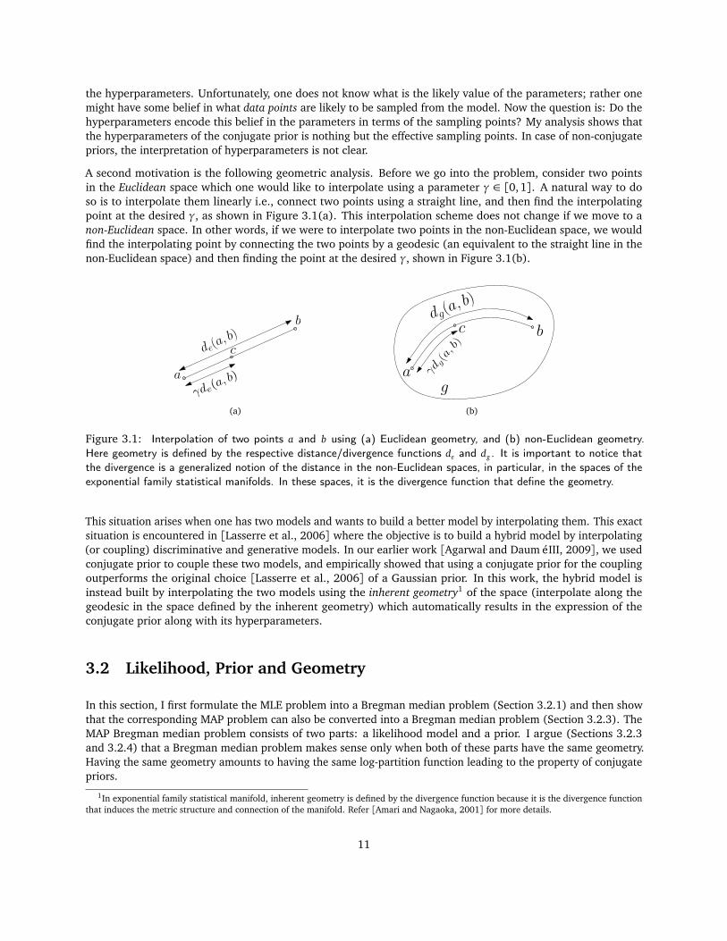
A second motivation is the following geometric analysis. Before we go into the problem, consider two pointsin the Euclidean space which one would like to interpolate using a parameter γ ∈ [0,1]. A natural way to doso is to interpolate them linearly i.e., connect two points using a straight line, and then find the interpolatingpoint at the desired γ, as shown in Figure 3.1(a). This interpolation scheme does not change if we move to anon-Euclidean space. In other words, if we were to interpolate two points in the non-Euclidean space, we wouldfind the interpolating point by connecting the two points by a geodesic (an equivalent to the straight line in thenon-Euclidean space) and then finding the point at the desired γ, shown in Figure 3.1(b).

a

c

b

de(a, b)

γde(a,

b)

(a)

bdg(a

, b)

γdg(a, b)

ga

c

(b)

Figure 3.1: Interpolation of two points a and b using (a) Euclidean geometry, and (b) non-Euclidean geometry.Here geometry is defined by the respective distance/divergence functions de and dg . It is important to notice thatthe divergence is a generalized notion of the distance in the non-Euclidean spaces, in particular, in the spaces of theexponential family statistical manifolds. In these spaces, it is the divergence function that define the geometry.

This situation arises when one has two models and wants to build a better model by interpolating them. This exactsituation is encountered in [Lasserre et al., 2006] where the objective is to build a hybrid model by interpolating(or coupling) discriminative and generative models. In our earlier work [Agarwal and Daumé III, 2009], we usedconjugate prior to couple these two models, and empirically showed that using a conjugate prior for the couplingoutperforms the original choice [Lasserre et al., 2006] of a Gaussian prior. In this work, the hybrid model isinstead built by interpolating the two models using the inherent geometry1 of the space (interpolate along thegeodesic in the space defined by the inherent geometry) which automatically results in the expression of theconjugate prior along with its hyperparameters.

3.2 Likelihood, Prior and Geometry

In this section, I first formulate the MLE problem into a Bregman median problem (Section 3.2.1) and then showthat the corresponding MAP problem can also be converted into a Bregman median problem (Section 3.2.3). TheMAP Bregman median problem consists of two parts: a likelihood model and a prior. I argue (Sections 3.2.3and 3.2.4) that a Bregman median problem makes sense only when both of these parts have the same geometry.Having the same geometry amounts to having the same log-partition function leading to the property of conjugatepriors.

1In exponential family statistical manifold, inherent geometry is defined by the divergence function because it is the divergence functionthat induces the metric structure and connection of the manifold. Refer [Amari and Nagaoka, 2001] for more details.

11

3.2.1 Likelihood in the form of Bregman Divergence

Let X be the input data space, and Θ be the parameter space such that for each θ ∈Θ, p(x;θ) is an exponentialfamily distribution as defined in (2.5) (the likelihood of the point x ∈ X under distribution given by θ). Following[Collins et al., 2001], we can write the log likelihood of exponential family distributions in terms of Bregmandivergence :

log p(x;θ) = log po(x) + F(φ(x))− BF (φ(x)‖∇G(θ)) (3.1)

This relationship depends on two observations: F(∇G(θ)) + G(θ) = ⟨∇G(θ),θ ⟩ and (∇F)−1(θ) = ∇G(θ)⇒(∇F)(∇G(θ )) = θ . These two observations can be used with (2.3) to see that (3.1) is equivalent to the probabilitydistribution defined in (2.5). This representation of likelihood in the form of Bregman divergence gives insight inthe geometry of the likelihood function.

In learning problems, one is interested in estimating the parameters θ of the model which results in lowgeneralization error, and perhaps, the most standard estimation method is maximum likelihood, which solves thefollowing problem:

Definition 1. MLE. Given a set of data points Xn and a family of distribution p(x;θ ) parametrized by θ ∈ Rd , MLEfinds θ̂M L ∈Θ such that θ̂M L = arg maxθ∈Θ

∑ni=1 log p(x i;θ).

It turns out that for exponential family distributions, the MLE problem can be transformed into a geometricproblem, in particular into a Bregman median problem.

Lemma 1. Let Xn be a set of n i.i.d. training data points drawn from the exponential family distribution with thelog partition function G, and F be the dual function of G. Then the dual of the MLE (θ̂M L) of Xn under the assumedexponential family model solves the following Bregman median problem:

θ̂ ∗M L = µ̂M L = arg minµ∈M

n∑

i=1

BF (φ(x i)‖µ) (3.2)

Proof. The log-likelihood of Xn under the assumed exponential family distribution is given by log p(Xn;θ) =∑n

i=1 log p(x i;θ) which along with (3.1) can be used to compute MLE i.e., θ̂M L:

θ̂M L = argmaxθ∈Θ

n∑

i=1

�

log po(x i) + F(φ(x i))− BF (φ(x i)‖∇G(θ))�

= argminθ∈Θ

n∑

i=1

BF (φ(x i)‖∇G(θ)) (3.3)

which using ∇G(θ) = µ, takes the entire problem into the M-space and gives the desired result.

The above theorem converts the problem of maximizing the log likelihood log p(Xn;θ) into an equivalentproblem of minimizing the corresponding Bregman divergences which is nothing but a Bregman median problem,the solution to which is given by µ̂M L =

1n

∑ni=1φ(x i). MLE θ̂M L can now be computed using the expression

∇G(θ) = µ, θ̂M L = (∇G)−1(µ̂M L).

Corollary 1 (MLE for Single Point). Let x i be the only point observed, µ̂i,M L under this observed point is φ(x i).

Proof. In Lemma 1, for single point, (3.2) is minimized when µ̂i,M L = φ(x i).

Unless otherwise stated, I will use µi instead of µ̂i,M L to make notations less cluttered.

12

µ1 µn

Mµ̂ML

BF (µ1||µ)

m-affine

θ1θn

θ̂ML

Θ

BG(θ||θ1)e-affine

Figure 3.2: MLE as Bregman median problem into Θ and M spaces for exponential family distributions. In Θspace, it is a problem over θis with optimal θ appearing in the first argument of the divergence function while inM-space, it is a problem over mean parameters with optimal µ appearing in the second argument in the divergencefunction.

Theorem 1 (MLE as Bregman Median). Let M and Θ be dual spaces as defined earlier, θi be the MLE of data pointx i under the exponential family parametric model p(x;θ) with log partition function G(θ). Given such {θ1, . . . ,θn}for all points {x1, . . . , xn}, θ̂M L is equivalent to:

θ̂M L = argminθ∈Θ

n∑

i=1

BG(θ‖θi) (3.4)

Proof. From Corollary 1, φ(x i) = µi , now replacing this in (3.2) gives µ̂M L = arg minµ∈M∑n

i=1 BF (µi‖µ). Now forµ1,µ2 ∈M and θ1,θ2 ∈ θ , using the relationship BF (µ1‖µ2) = BG(θ2‖θ1) takes the entire problem from M-spaceto Θ-space giving the desired result.

Figure 3.2 gives a pictorial summarization of these MLE(s) as Bregman median problems in Θ and M spaces.The above expression requires us to find a θ so that divergence from θ to other θi is minimized. Now note thatG is what defines this divergence and hence the geometry of the Θ space (as discussed earlier in Section 3.1).Since G is the log partition function of an exponential family, it is the log-partition function that determinesthe geometry of the space. I emphasize that divergence is measured from the parameter being estimated toother parameters θi(s), as shown in Figure 3.3.

3.2.2 Conjugate Prior in the form of Bregman Divergence

An expression similar to the likelihood can be written for the conjugate prior:

log p(θ |α,β) = log m(α,β) + β(⟨θ ,α

β⟩ − G(θ)) (3.5)

(3.5) can be written in the form of Bregman divergence by a direct comparison to (2.5), replacing φ(x) with α/β .

log p(θ |α,β) = log m(α,β) + β�

F�

α

β

�

− BF

�

α

β‖∇G(θ)

��

(3.6)

13

The expression for the joint probability of data and parameters is given by:

log p(x ,θ |α,β) = log po(x) + log m(α,β) + F(φ(x)) + βF�

α

β

�

−�

BF (φ(x)‖∇G(θ)) + βBF

�

α

β‖∇G(θ)

��

Combining all terms that do not depend on θ :

log p(x ,θ |α,β) = const− BF (φ(x)‖µ)− βBF

�

α

β‖µ�

(3.7)

3.2.3 Geometric Interpretation of Conjugate Prior

In this section I give a geometric interpretation of the term BF (φ(x)‖µ) + βBF (α

β‖µ) from (3.7).

Theorem 2 (MAP as Bregman median). Given a set Xn of n i.i.d. examples drawn from the exponential familydistribution with the log partition function G and a conjugate prior as in (3.6), MAP estimation of parameters isθ̂MAP = µ̂∗MAP where µ̂MAP solves the following problem:

µ̂MAP = arg minµ∈M

n∑

i=1

BF (φ(x i)‖µ) + βBF

�

α

β‖µ�

(3.8)

which admits the following solution:

µ̂MAP =

∑ni=1φ(x i) +α

n+ β

Proof. MAP estimation by definition maximizes (3.7) for all data points Xn which is equivalent to minimizingBF (x i‖µ) + βBF (

α

β‖µ). One can expand this expression using (2.3) and use conditions F(∇G(θ)) + G(θ) =

⟨∇G(θ),θ ⟩ and (∇F)−1(θ) =∇G(θ) to obtain the desired solution.

The above solution gives a natural interpretation of MAP estimation. One can think of prior as β number ofextra points at position α/β . β works as the effective sample size of the prior which is clear from the followingexpression of the dual of the θ̂MAP :

µ̂MAP =

∑ni=1φ(x i) +

∑β

i=1α

β

n+ β(3.9)

The expression (3.8) is analogous to (3.2) in the sense that both are defined in the dual space M. One can convert(3.8) into an expression similar to (3.4) in the dual space which is again a Bregman median problem in theparameter space.

θ̂MAP = argminθ∈Θ

n∑

i=1

BG(θ‖θi) +β∑

i=1

BG

�

θ‖(α

β)∗�

(3.10)

here ( αβ)∗ ∈ Θ is dual of α

β. The above problem is a Bregman median problem consisting of n + β points,

{θ1,θ2 . . .θn, (α/β)∗, . . . , (α/β)∗︸ ︷︷ ︸

β times

}, as shown in Figure 3.3 (left).

14

A geometric interpretation is also shown in Figure 3.3. When the prior is conjugate to the likelihood, they bothhave the same log-partition function (Figure 3.3, left). Therefore they induce the same Bregman divergence.Having the same divergence means that distances from θ to θi (in likelihood) and the distances from θ to (α/β)∗

are measured with the same divergence function, yielding the same geometry for both spaces.

It is easier to see using the median formulation of the MAP estimation problem that one must choose a prior thatis conjugate. If one chooses a conjugate prior, then the distances among all points are measured using the samefunction. It is also clear from (3.9) that in the conjugate prior case, the point induced by the conjugate priorbehaves as a sample point (α/β)∗. A median problem over a space that have different geometries is an ill-formedproblem, as discussed further in the next section.

3.2.4 Geometric Interpretation of Non-conjugate Prior

The expression (3.10) was considering the prior to be conjugate to the likelihood function. Had the prior beennon-conjugate with the log-partition function e.g., Q, one would have instead obtained:

θ̂M L =minθ∈Θ

n∑

i=1

BG(θ‖θi) +β∑

i=1

BQ

�

θ ‖�

α

β

�∗�

. (3.11)

Here G and Q are different functions defined over Θ. Since these are the functions that define the geometry of thespace parameter, having G 6= Q is equivalent to consider them as being defined over different (metric) spaces.Here, it should be noted that distance between the sample point (θi) and the parameter θ is measured using theBregman divergence BG . On the other hand, the distance between the point induced by the prior (α/β)∗ and θis measured using the divergence function BQ. This means that (α/β)∗ can not be treated as one of the samplepoints. This tells us that, unlike the conjugate case, belief in the non-conjugate prior can not be encoded in theform of the sample points.

Another problem with considering a non-conjugate prior is that the dual space of Θ under different functionswould be different. Thus, one will not be able to find the alternate expression for (3.11) equivalent to (3.8), andtherefore not be able to find the closed-form expression similar to (3.9). This tells us why non-conjugate does notgive us a closed form solution for θ̂MAP . A pictorial representation of this is also shown in Figure 3.3. Note that,unlike the conjugate case, in the non-conjugate case, the data likelihood and the prior both belong to differentspaces.

I emphasize that it is possible to find the solution of (3.11) i.e., in practice, there is nothing that prohibits theuse of non-conjugate prior, using the conjugate prior is intuitive, and allows one to treat the hyper-parameters aspseudo data points.

3.3 Hybrid model

In this section, I show an application of the above analysis to a common supervised and semi-supervised learningframework, in particular, to a generative/discriminative hybrid model [Agarwal and Daumé III, 2009,Druck et al.,2007,Lasserre et al., 2006] that has been shown to be successful in many applications.

The hybrid model is a mixture of discriminative and generative models, each of which has its own separate set ofparameters. These two sets of parameters (hence two models) are combined using a prior called the coupling prior.Let p(y|x,θd) be the discriminative component, p(x, y|θg) be the generative component and p(θd ,θg) be the prior

15

θ1

θ2 θ̂

{(αβ)∗}β

Rd θ1

θ2θ̂

RdConjugateNon-conjugate

{(αβ)∗}βBG(θ

‖θ1)

BG(θ‖θ

2 ) BG (θ‖( α

β ) ∗) BG(θ‖θ1

)

BG (θ‖θ

2 )

BQ(θ‖( α

β ) ∗)

Figure 3.3: Prior in the conjugate case has the same geometry as the likelihood while in the non-conjugate case, theyhave different geometries.

that couples discriminative and generative components. The joint likelihood of the data and parameters is:

p(x, y,θd ,θg) = p(θg ,θd)p(y|x,θd)p(x|θg) (3.12)

= p(θg ,θd)p(y|x,θd)∑

y ′p(x, y ′|θg)

here θd is a set of discriminative parameters, θg a set of generative parameters, and p(θg ,θd) provides the naturalcoupling between these two sets of parameters.

The most important aspect of this model is the coupling prior p(θg ,θd), which interpolates the hybrid modelbetween two extremes: fully generative when the prior forces θd = θg , and fully discriminative when the priorrenders θd and θg independent. In non-extreme cases, the goal of the coupling prior is to encourage the generativemodel and the discriminative model to have similar parameters. It is easy to see that this effect can be induced bymany functions. One obvious way is to linearly interpolate them as done by [Lasserre et al., 2006,Druck et al.,2007] using a Gaussian prior (or the Euclidean distance) of the following form:

p(θg ,θd)∝ exp�

−λ�

�

�

�θg − θd

�

�

�

�

2�

(3.13)

where, when λ= 0, model is purely discriminative while for λ=∞, model is purely generative. Thus λ in theabove expression is the interpolating parameter, and is same as the γ in Section 3.1. Note that the log of the prioris nothing but the squared Euclidean distance between two sets of parameters.

It has been noted multiple times [Bouchard, 2007, Agarwal and Daumé III, 2009] that a Gaussian prior is notalways appropriate, and the prior should instead be chosen according to models being considered. In our earlierwork [Agarwal and Daumé III, 2009], we suggested using a prior that is conjugate to the generative model. Ourmain argument for choosing the conjugate prior came from the fact that this provides a closed form solutionfor the generative parameters and therefore is mathematically convenient. In this work, I will show that it ismore than convenience that makes conjugate prior appropriate by using their geometric interpretation studiedin the previous section. In addition to providing a justification behind their use as a coupling prior, this analysisalso derives the expression and hyperparameters of the prior automatically (an additional advantage of usinggeometric methods).

16

θd

θg

Θd Θg

BG(θg‖θd)

λ

Figure 3.4: Parameters θd and θg are interpolated using the Bregman divergence

3.3.1 Generalized Hybrid Model

In order to see the effect of geometry, I first present the generalized hybrid model for distributions that belongto the exponential family and present them in the form of Bregman divergences. Following the expression usedin [Agarwal and Daumé III, 2009], the generative model can be written as:

p(x, y|θg) = h(x, y)exp(⟨θg , T (x, y)⟩ − G(θg)) (3.14)

where T (·) is the potential function similar to φ in (2.5), now only defined on (x, y).

Let G∗ be the dual function of G; the corresponding Bregman divergence (retaining only the terms that depend onthe parameter θ) is given by:

BG∗�

(x, y)‖∇G(θg)�

. (3.15)

Solving the generative model independently reduces to choosing a θg from the space of all generative parametersΘg which has a geometry defined by the log-partition function G. Similarly to the generative model, the exponentialform of the discriminative model is given as:

p(y|x,θd) = exp(⟨θd , T (x, y)⟩ −M(θd ,x)) (3.16)

Importantly, the sufficient statistics T are the same in the generative and discriminative models; such genera-tive/discriminative pairs occur naturally: logistic regression/naive Bayes and hidden Markov models/conditionalrandom fields are examples. However, observe that in the discriminative case, the log partition function M dependson both x and θd which makes the analysis of the discriminative model harder. Unlike the generative model, onedoes not have the explicit form of the log-partition function M that is independent of x. This means that thediscriminative component (3.16) can not be converted into an expression like (3.15), and the MLE problem cannot be reduced to the Bregman median problem like the one given in (3.4).

3.3.2 Geometry of the Hybrid Model

The analysis of the hybrid model is simplified by writing the discriminative model in an alternate form. Thisalternate form makes obvious the underlying geometry of the discriminative model. Note that the only differencebetween the two models is that discriminative model models the conditional distribution while the generativemodel models the joint distribution. This observation can be used to write the discriminative model in thefollowing alternate form using the expression p(y|x ,θ) = p(y,x |θ)

∑

y′ p(y ′ x |θ) and (3.14):

p(y|x ,θd) =h(x, y)exp(⟨θd , T (x, y)⟩ − G(θd))

∑

y ′ h(x, y ′)exp(⟨θd , T (x, y ′)⟩ − G(θd))(3.17)

17

Denote the space of parameters of the discriminative model by Θd . It is easy to see that geometry of Θd is definedby G since function G is defined over θd . This is same as the geometry of the parameter space of the generativemodel Θg . Now let us define a new space ΘH which is the affine combination of Θd and Θg . Now, ΘH will havethe same geometry as Θd and Θg i.e., geometry defined by G. Now the goal of the hybrid model is to find aθ ∈ ΘH that maximizes the likelihood of the data under the hybrid model. These two spaces are shown pictoriallyin Figure 3.4.

3.3.3 Prior Selection

As mentioned earlier, the coupling prior is the most important part of the hybrid model, which controls theamount of coupling between the generative and discriminative models. There are many ways to do this, one ofwhich is given by [Lasserre et al., 2006,Druck et al., 2007]. By their choice of Gaussian prior as coupling prior,they implicitly couple the discriminative and generative parameters by the squared Euclidean distance. I suggestcoupling these two models by a general prior, of which the Gaussian prior is a special case.

Bregman Divergence and Coupling Prior: Let a general coupling be given by BS(θg‖θd). Notice the directionof the divergence. This direction was chosen because the prior is induced on the generative parameters, and it isclear from (3.10) that parameters on which prior is induced, are placed in the first argument in the divergencefunction. The direction of the divergence is also shown in Figure 3.4.

Now recall the relation (3.6) between the Bregman divergence and the prior. Ignoring the function m (this isconsumed in the measure defined on the probability space) and replacing ∇G(θ) by θ ∗, we get the followingexpression:

log p(θg |α,β) = β(F(α

β)− BF (

α

β‖θ ∗g )) (3.18)

Now taking the α= λθ ∗d and β = λ, we get:

log p(θg |λθ ∗d ,λ) = λ(F(θ ∗d )− BF (θ∗d‖θ

∗g )) (3.19)

p(θg |λθ ∗d ,λ) = exp(λ(F(θ ∗d ))) exp(−λBF (θ∗d‖θ

∗g )) (3.20)

For the general coupling divergence function BS(θg‖θd), the corresponding coupling prior is given by:

exp(−λBS∗(θ∗d‖θ

∗g )) = exp(−λ(F(θ ∗d ))) p(θg |λθ ∗d ,λ) (3.21)

The above relationship between the divergence function (left side of the expression) and coupling prior (right sideof the expression) allows one to define a Bregman divergence for a given coupling prior and vise versa.

Coupling Prior for the Hybrid Model: It is known that that the geometry of the space underlying the Gaussianprior is just Euclidean, which does not necessarily match the geometry of the likelihood space. The relationshipbetween prior and divergence (3.21) allows one to first define the appropriate geometry for the model, and thendefine the prior that respects this geometry. In the above hybrid model, this geometry is given by the log partitionfunction G of the generative model. This argument suggests to couple the hybrid model by the divergence of theform BG(θg‖θd). The coupling prior corresponding to this divergence function can be written using (3.21) as:

exp(−λBG∗(θd∗‖θg

∗)) = p(θg |λθd∗,λ) exp(−λF(θ ∗d )) (3.22)

where λ = [0,∞] is the interpolation parameter, interpolating between the discriminative and generative extremes.In dual form, the above expression can be written as:

exp(−λBG(θg‖θd)) = p(θg |λθd∗,λ) exp(−λF(θ ∗d )). (3.23)

18

Here exp(−λF(θd∗)) = exp(λ(G(θd)− θd∇G(θd))) can be thought of as a prior on the discriminative parameters

p(θd). In the above expression, exp(−λBG(θg‖θd)) = p(θg |θg)p(θd) behaves as a joint coupling prior P(θd ,θg) asoriginally expected in the model (3.12). Note that hyperparameters of the prior α and β are naturally derivedfrom the geometric view of the conjugate prior. Here α= λθ ∗d and β = λ.

3.4 Related Work and Conclusion

To the best of my knowledge, there have been no previous attempts to understand Bayesian priors from a geometricperspective. However, one related piece of work [Snoussi and Mohammad-Djafari, 2002] uses the Bayesianframework to find the best prior for a given distribution. It is noted that, in that work, the authors use theδ-geometry for the data space and the α-geometry for the prior space, and then show different cases for differentvalues (δ,α). It is emphasized that even though it is possible to use different geometry for the both spaces, italways makes more sense to use the same geometry. As mentioned in remark 1 in [Snoussi and Mohammad-Djafari,2002], useful cases are obtained only when we consider the same geometry.

In this chapter, I have shown how geometry and the methods derived from it, are useful to get a better understand-ing of existing models. More specifically, I have considered the geometry underlying the model space and used it totransform the MLE problem into a geometric problem, Bregman median problem. This geometric interpretation ofthe space and the likelihood function allowed me to reason about the conjugate prior beyond their mathematicalconvenience. In addition to providing an insight in the hybrid model, this interpretation also justified the use ofconjugate prior as a coupling prior; and as an added advantage, derived the expression and the hyperparametersof this coupling prior.

19

Chapter 4

Generative Kernels

In this chapter, I use geometric methods to build a family of kernels that can be used as off-the-shelf tool for anykernel learning method such as support vector machines. Generative models provide a useful statistical languagefor describing data; discriminative methods achieve excellent classification performance. In this chapter, I usegeometric understanding of generative models to propose a family of kernels i.e., generative kernels, defined as afamily of kernels built around generative models for use in discriminative classifiers. The key idea of generativekernels is to use the generative model of the data to automatically define a statistical manifold, on which aparticular natural divergence (based on the Fisher information metric) can be translated into a positive definitekernel. My approach is applicable to any statistical model belonging to the exponential family, which includescommon distributions like the Gaussian and multinomial, as well as more complex models.

Apart from the geometric perspective, there are other reasons to consider the data distribution when constructingthe kernels. It is commonly observed that generative models perform well when only a small amount of datais available [Ng and Jordan, 2001], especially when the model is a true model of the data distribution [Liangand Jordan, 2008]. However, as the model becomes less true, or as the amount of data grows, discriminativeapproaches prevail, both theoretically and empirically [Ng and Jordan, 2001,Liang and Jordan, 2008]. Ideally,one would like to take advantage of both methods, and build a hybrid method, that performs well for smalltraining data and does not rely too much on the generative assumption. One way to build such a hybrid model isto combine discriminative and generative models using a coupling prior as I described in the previous chapter.Another way to build hybrid model is to encode the generative process information in the kernel and then use thiskernel in the discriminative method.

There have been previous efforts to build kernels from generative models: the Fisher kernel [Jaakkola andHaussler, 1999], the heat kernel [Lafferty and Lebanon, 2005], and the probability product (PP) kernel [Jebaraet al., 2004]. The first two consider the generative process by deriving the geometry for the statistical manifoldassociated with the generative distribution family using the fundamental principle of the information distance.Unfortunately, these kernels are intractable to compute exactly even for very simple distributions due to the needto compute the Fisher information metric. The approximations required to compute these kernels result in afunction that is not guaranteed to be positive definite [Martins et al., 2008]. More discussion on the related workcan be found in our published work [Agarwal and Daumé III, 2011]. There is another family of kernels namedsemi-group kernels [Cuturi et al., 2005] which turns out to have the same functional form as generative kernelsthough both are derived completely differently. Unlike [Cuturi et al., 2005], I consider the geometry of the datadistribution and reason why it is appropriate to call these kernels generative kernels. Note that semi-group kernelsare not generative kernels for general probability distributions therefore empirical study of these kernels underthe discriminative/generative paradigm is not considered in [Cuturi et al., 2005]. In this chapter, generativekernels are studied under generative/discriminative paradigm, in particular, experiments are performed to see

20

0 20 40 60 80 100 120 140 160 180 2000.05

0.1

0.15

0.2

0.25

0.3

0.35

0.4

0.45

Training examples per classC

lass

ifica

tion

erro

r

student vs. project

Exp

Inverse

PP

Heat

NB

Figure 4.1: A typical example of relative performance on real dataset from multinomial distribution. Exp and Inverse are thegenerative kernels.

what happens when the data generation assumption is violated i.e., when the model is mis-specified.

These generative kernels have a number of desirable properties:

• They are applicable to any exponential family distribution.

• They are built using the natural geometry of the model space associated with data distribution.

• They are closed-form, efficient to compute, and by construction are always positive definite.

• Empirical comparisons to the best published kernels using the same data and experimental setup showimproved performance.

• Empirical results with these kernels show that these kernels are able to exploit the generative properties i.e.,perform as well as a generative model when there is less training data.

Unlike other distribution-based kernels, a discriminative method based on the proposed generative kernel is able toexploit the properties of the generative methods i.e., perform well when not enough data is given. Figure 4.1 showstypical result from a real world classification task on the text data. The blue curve which represents the generativemethod (Naive Bayes (NB)) performs better when training size n is small but as n is increased, discriminativemethods (other curves) start to take over. Although other discriminative methods perform poorer than the NB forsmall n, discriminative methods when used with generative kernel, perform better for all n. Generative kernels(red and green curves) perform equal/better to NB when n is small, and outperform all other methods as n getslarge. Generative kernel curves are lower envelopes of all other curves, giving us the best of both worlds.

4.1 Background: Statistical Manifolds and Dualistic Structure

In this section, I define statistical manifolds and the dualistic structure associated with them. I in particular givereasons why it is important to choose the KL divergence to define the kernel for the exponential family. A statisticalmanifold S is a d-dimensional manifold S = {θ ∈Θ} such that every θ ∈Θ induces a probability distributionover some space X.

21

Following [Amari and Nagaoka, 2001], it is well known that all arbitrary divergences induce a dualistic structureand a metric. In particular, for statistical manifolds, the most natural divergence is the one that induces theFisher information metric. The Fisher information metric is a special Reimannian metric that has many attractiveproperties (e.g. invariance under reparameterization), and is considered to be a natural metric for statisticalmanifolds. A divergence function that induces the Fisher information metric on the exponential family manifolds isK L divergence. It is also known as D−1 divergence (a special case of Dη divergence for η =−1). Since exponentialfamily manifolds have dualistic structure (in fact they are dually flat), there exists a dual space, where one candefine the dual divergence i.e. D1 divergence. Following [Zhang, 2004], this duality is called referential duality.In referential duality, for two points p, q ∈Θ D−1(p‖q) = D1(q∗‖p∗) or K L(p‖q) = K L∗(q∗‖p∗). For exponentialfamily statistical manifold, this duality is closely related to the other form of duality i.e., Legendre duality, and isalso known as representational duality; and in such duality, BF (p‖q) = BG(q∗‖p∗), where F and G are dual of eachother.

4.2 Generative Model to Metric

In this section, I develop generative kernels. I first take the Bregman median problem corresponding to theexponential family distribution that generated the data, and transform it into a problem that minimizes the KLdivergence in Θ-space. As mentioned above, a natural divergence in Θ-space is the K L divergence. I use this K Ldivergence to build a metric in Θ-space. Using duality, this metric is projected into M-space, and then finally inthe Section 4.3, this projected metric is converted into a positive definite kernel.

Here, I first borrow the Bregman median problem from Section 3.2.1 corresponding to the generative modelbelonging to the exponential family. Recall, the Bregman median problem is:

θ̂M L = argminθ∈Θ

n∑

i=1

BG(θ‖θi)

where M and Θ are dual spaces of each other as defined earlier, and {θ1, . . . ,θn} are the MLE of data points{x1, . . . , xn}, under the exponential family model p(x;θ). Now this Bregman median problem in Θ-space can betransformed into a K L minimization problem using the following Lemma.

Lemma 2 (KL and Bregman for Exponential Family). Let K L(θ1‖θ2) be the KL divergence for θ1,θ2 ∈ Θ, thenK L(θ1‖θ2) = BG(θ2‖θ1)

Proof. This directly follows from the definitions of KL divergence and exponential family; and from the relation,Eθ (x) =∇G(θ) for exponential family.

Theorem 3. MLE θ̂M L of data points Xn generated from exponential family is now given by:

θ̂M L = arg minθ∈Θ

n∑

i=1

K L(θi‖θ) (4.1)

Proof. From Lemma 2, K L(θi‖θ) = BG(θ‖θi), substituting this in (3.4) gives the desired result.

In (4.1), It is worth nothing that the parameter being estimated comes in the second argument of K L divergence.This observation along with the following definition is used to construct a metric in Θ-space.

Definition 2 (JS Divergence). For θ1,θ2 ∈Θ and θ̃ = (θ1+θ2)2

, JS(θ1,θ2) is defined as:

JS(θ1,θ2) =1

2

�

K L(θ1‖θ̃) + K L(θ2‖θ̃)�

22

It is well known thatp

JS is a metric.p

JS have also been shown to be Hilbertian [Fuglede and Topsoe,2004, Berg et al., 1984]. A metric d(x , y) is said to be Hilbertian metric if and only if d2(x , y) is a negativedefinite(n.d.) [Schoenberg, 1938]. Since

pJS is a Hilbertian metric, JS is n.d..

It is important to understand the purpose of the above analysis in deriving the metric based on the JS divergence.I will call this metric as JS metric. This analysis builds a bridge between the JS metric and the generativemodels. The JS metric can therefore be used to build kernels that can exploit the generative properties of the data.Establishing the connection between the JS metric and the generative models in theory, and showing the efficacyof the kernels based on this metric in practice, is the main contribution of this chapter.

The JS metric, which is based on symmetrized KL divergence has been known for a long time [Cuturi et al., 2005].However, what is not known is the generative behavior of the JS metric. In the existing literature, JS metric isusually derived for any probability distribution, and for a general probability distribution, JS metric does notconsider the generative model of the data, and therefore can not be used to build generative kernels. I, in thiswork, only consider the distributions belonging to the exponential families, for which, the JS metric can be shownto have been derived considering the generative model. This connection between the JS metric and the generativemodel allows us to build kernels that can be used to build hybrid models.

Definition 3 (Dual JS Divergence). For µ1,µ2 ∈M and µ̃ = (µ1+µ2)2

, let K L∗(.‖.) be the dual of K L divergencethen the dual JS divergence DJS(µ1,µ2) is defined as:

DJS(µ1,µ2) =1

2

�

K L∗(µ̃‖µ1) + K L∗(µ̃‖µ2)�

Theorem 4. DJS is negative definite.

Proof. Result is direct consequence of the fact that JS divergence is symmetric. Using the relationship betweenK L and K L∗, one can simply take the dual of JS which is DJS(θ1,θ2) =

12(K L(θ1‖θ̃) + K L(θ2‖θ̃)) = JS(θ1,θ2)

which is n.d..

Theorem 5. Let ψ(µ1,µ2) = DJS(µ1,µ2) be a n.d. function on M, then

ψ(µ1,µ2) =F(µ1) + F(µ2)

2− F�µ1 +µ2

2

�

(4.2)

Proof. Using the duality, K L∗(µ1‖µ2) = BF (µ2‖µ1); DJS(µ1,µ2) =12(BF (µ1‖µ̃) + BF (µ2‖µ̃)). Expanding the

expression for the Bregman divergence and using some algebra yields the result.

Though not analyzed, this expression is also observed in [Chen et al., 2008]. It is to be noted that this metric(4.2) is defined over the mean parameters, so in order to define the metric over the data points Xn, one can useCorollary 1, according to which, ψ(µ1,µ2) =ψ(φ(x1),φ(x2)). Recall φ(x) here is the sufficient statistics.

4.3 Metric to Kernel

In this section, I convert the previously constructed Hilbertian metric (n.d. function) into a family of kernels thatwill be used later in the experiments. I now state some results that can be used along with (4.2) to build thekernels called “generative kernels“. Although there could be many ways [Berg et al., 1984,Schoenberg, 1938] totransform a metric into a kernel, I mention a few here:

23

Proposition 1 (Centering). Let function ψ : X×X→ R be a symmetric function, and x0 ∈ X. Let ϕ : X×X→ Rbe

ϕ(x , y) =ψ(x , x0) +ψ(y, x0)−ψ(x , y)−ψ(x0, x0),

then ϕ is n.d. if and only if ψ is positive definite (p.d.).

Proposition 2 (Exponentiated(Exp)). The function ψ : X×X→ R is n.d. if and only if exp(−tψ) is p.d. for allt > 0.

Proposition 3 (Inverse). The function ψ : X×X→ R is n.d. if and only if (t +ψ)−1 is p.d. for all t > 0.

Note that the computation complexity of generative kernels depends on the computational complexity of the dualof log-patition function.

4.4 Preliminary Experiments

In this section I evaluate generative kernels on several text categorization tasks (multinomial distributions), as afirst evidence of their effectiveness. Later in the proposed work, I plan to apply them for more complex models(tasks). In my preliminary experiments, I use multinomial distribution for this evaluation – mainly for two reasons.First, multinomial is one of the most widely used distributions after Gaussian1. Second, other principally similarkernels which I would like to compare against, have been shown to work only for the multinomial geometry, forcomputational reasons. Note that for multinomial distribution, φ(x) is simply the observed frequency vector.

I have performed experiments with six kernels: generative(centering, exp and inverse), linear, Heat and PP kernels.In these experiments, generative kernels are compared with some of the best published results for multinomialdistribution i.e., heat and PP kernel. In order to see the discriminative/generative behavior, I also include theresults of a generative model (NB with α-smoothing). In order to make graphs look less cluttered, I excludegenerative centering and linear kernels. In most of the cases they underperformed other kernels. For statisticalsignificance, all of the results are averaged over 20 runs. Although in my results, I only report the mean error,variance was found to be very low (∼ 0.0001), and hence not reported for the clarity. For evaluation, I use SVMtoolbox [Canu et al., 2005].

Here I report results on the synthetic data (generated from multinomial distribution) because these are moreintuitive and give insight into hybrid behavior. I have also performed experiments on real datasets mainly textclassification tasks (i.e. multinomial distribution) which can be found in our published work [Agarwal and DauméIII, 2011].

For the multinomial distribution, the relative size of each trial w compared to the dimension of the data d isimportant because that’s what makes problems difficult or easier. if multinomial distributions are considered to bethe documents, then long documents compared to the vocabulary size(low d/w, dense setting) makes problemeasier while short documents (high d/w, sparse settings) makes the problem difficult. I show results for bothdense and sparse settings. For each of these settings, I perform two kind of experiments, In one n is varied (nonoise), and in other the noise level( n = 50) is varied. Noise is introduced by copying the result of previoustrial with probability p =noise level. In sparse setting d/w = 100 while in dense d/w = 5 with w = 20. Theseresults are shown in Figure 4.2 and Figure 4.3 respectively. Since in all of these experiments, generative kernelsoutperform other kernel methods, an important comparison would be to see how a method based on generativekernels performs compared to a pure generative method (NB) mainly because discriminative models based ongenerative kernels can be thought of as a mixture of discriminative/generative models.

In all of these experiments, results are found to be interesting and consistent with previous known facts. In thenon-noise dense settings, it is observed that generative kernels based method outperforms all other methods

1Gaussian is uninteresting because all kernels, heat, PP and generative reduce to RBF

24

0 20 40 60 80 1000.05

0.1

0.15

0.2

0.25

0.3

0.35

0.4

0.45

Training examples per class

Cla

ssifi

catio

n er

ror

Dense data (Simple)

Exp

Inverse

PP

Heat

NB

0 20 40 60 80 1000.1

0.2

0.3

0.4

0.5

0.6

0.7

0.8

Training examples per class

Cla

ssifi

catio

n er

ror

Sparse data (Hard)

Exp

Inverse

PP

Heat

NB

Figure 4.2: Performance variation with n on random multinomial dataset in sparse and dense settings

0 0.1 0.2 0.3 0.4 0.5 0.6 0.7 0.80.05

0.1

0.15

0.2

0.25

0.3

0.35

0.4

Noise level

Cla

ssifi

catio

n er

ror

Dense data (simple)

Exp

Inverse

PP

Heat

NB

0 0.1 0.2 0.3 0.4 0.5 0.6 0.7 0.8

0.2

0.25

0.3

0.35

0.4

0.45

0.5

Noise level

Cla

ssifi

catio

n er

ror

Sparse data (hard)

Exp

Inverse

PP

Heat

NB

Figure 4.3: Performance variation with different noise levels on random multinomial dataset in sparse and densesettings

except for NB. It is known [Liang and Jordan, 2008] that in case of correct model assumption, generative modelsoutperform discriminative methods hence in this case, one can not hope to beat NB, though it beats all otherdiscriminative models for all n. It is also emphasized that when n is small generative kernels based methodperforms as well as the NB because for small n, generative properties dominate discriminative properties, but aswe increase the data, discriminative properties tend to dominate and model starts to perform poor. Similar resultsare obtained for the sparse setting except that problem is now harder, and for hard problem, relative differencebetween generative and discriminative is not very high.

An interesting phenomena occurs when I introduce noise, or when the model is mis-specified. Results are presentedin Figure 4.3. For simple problem (dense setting), NB outperforms all discriminative methods for all noise levels.In simple problem, introducing noise does not make much difference, and problem is still simple enough for NB toperform better, therefore, it is the hard problem that is more interesting. In hard problem (sparse setting), NBperforms better when there is less noise (∼ 10%), but as we increase the noise, correct model assumption breaksand generative kernels based method starts to outperform.

25

4.5 Conclusion and Future Work

In this chapter, I have used the geometric structure of the space associated with the generative models to build afamily of kernels called generative kernels that can be used as off-the-shelf tool in any kernel learning method.When used in discriminative models, these kernels exploit the properties of both, generative and discriminativemodels, giving us the best of both worlds. Empirical results demonstrate this hybrid behavior, in addition to thesuperior performance over the other state-of-the-art kernels.

Although in principle, generative kernels can be used for any exponential family models, I have yet to establishthe practical evidence. Many exponential family models can be represented as graphical models, and next studywould be to build generative kernels for such graphical models.

In the future work of this proposal, I plan to build generative kernels for the exponential families derived fromcomplex graphics model structures. Since the computation of these kernels requires the computation of the dualof the log partition function F , an important extension of this work is to study how to compute F . The plan is toconsider one task related to a graphical model, compute the dual of the log partition function F for the distributionassociated with that graphical model, and finally use this F to compute generative kernels. Although I plan tocompute these kernels for one specific graphical model problem, the main focus would be on building a generalframework that would allow one to compute these kernels for general graphical models.

26

Part II

Geoemetry in Data

27

Chapter 5

Universal Multidimensional Scaling

This chapter demonstrates the power of geometric methods by building a unified algorithmic framework to solvethe generalized multidimensional scaling (MDS) problem. By using simple tools from computational geometry, Iam able to build a framework that performs comparable to or better than the state-of-the-art methods for manyknown variants of MDS, and, at the same time, provides algorithms for the variants that have not yet beenstudied. In additional to superior performance, the algorithms derived from this geometry-driven framework havemany attractive properties i.e. they are simple, intuitive, easily parallelizable, and scale well to large data. Thisframework easily generalizes to the spaces other than the Euclidean space because it is based on simple geometricoperations such moving points in the space, intersection of line with surfaces etc., and a well known min-sumor centroid problem [Karcher, 1977, Buss and Fillmore, 2001], which is closely related to the facility locationproblem [Hochbaum, 1982,Bajaj, 1986], a problem well studied problem in theory and computational geometry.

5.1 Motivation

Multidimensional scaling (MDS) [Kruskal and Wish, 1978, Cox and Cox, 2000, Borg and Groenen, 2005] is awidely used method for embedding a general distance matrix into a low dimensional Euclidean space, used bothas a preprocessing step for many problems, as well as a visualization tool in its own right. MDS has been studiedand used in psychology since the 1930s [Young and Householder, 1938,Torgerson, 1952,Kruskal, 1964] to helpvisualize and analyze data sets where the only input is a distance matrix. More recently MDS has become astandard dimensionality reduction and embedding technique to manage the complexity of dealing with large highdimensional data sets [Cayton and Dasgupta, 2006,Chen and Buja, 2009,Pless and Simon, 2002,Bronstein et al.,2008].

In general, the problem of embedding an arbitrary distance matrix into a fixed dimensional Euclidean spacewith minimum error is nonconvex (because of the dimensionality constraint). Thus, in addition to the standardformulation [de Leeuw, 1977], many variants of MDS have been proposed, based on changing the underlyingerror function [Young and Householder, 1938,Cayton and Dasgupta, 2006]. There are also applications wherethe target space, rather than being a Euclidean space, is a manifold (e.g. a low dimensional sphere), and variousheuristics for MDS in this setting have also been proposed [de Leeuw and Mair, 2009,Bronstein et al., 2008]. Eachsuch variant is typically addressed by a different heuristic, including majorization [de Leeuw and Mair, 2009],the singular value decomposition [Torgerson, 1952], semidefinite programming [Cayton and Dasgupta, 2006],subgradient methods [Cayton and Dasgupta, 2006], and standard Lagrange-multipler-based methods (in bothprimal and dual settings) [de Leeuw and Mair, 2009]. Some of these heuristics are efficient, and others are not; ingeneral, every new variant of MDS seems to require different ideas for efficient heuristics.

28

In this chapter, I use geometric tools to build a unified algorithmic framework for solving many variants of MDS.My approach is based on an iterative local improvement method, and can be summarized as follows: “Pick apoint and move it so that the cost function is locally optimal. Repeat this process until convergence1.” Theimprovement step reduces to a well-studied and efficient family of iterative minimization techniques, where thespecific algorithm depends on the variant of MDS. This proposed method does not solve the optimization problemexplicitly, rather it breaks the problem into smaller subproblems where each subproblem can be solved by usingwell known geometric tools. The resulting algorithm is generic, efficient, and simple. The high level frameworkcan be written in 10-12 lines of MATLAB code, with individual function-specific subroutines needing only a fewmore lines each. A useful feature of this framework is that it is parameter-free, requiring no tuning parameters orLagrange multipliers in order to perform at its best. Further, this approach compares well with the best methodsfor all the variants of MDS, and scales to large data sets (because of small memory footprint), as we will see inChapter 7.

5.2 Background and Existing Methods

Multidimensional scaling is a family of methods for embedding a distance matrix into a low-dimensional Euclideanspace. There is a general taxonomy of MDS methods [Cox and Cox, 2000]; in this dissertation, I will focusprimarily on the metric and generalized MDS problems.

The traditional formulation of MDS [Kruskal and Wish, 1978] assumes that a given distance matrix D arises frompoints in some k-dimensional Euclidean space. Under this assumption, a simple transformation takes the distancematrix D to a matrix of similarities S = (si j), where si j = ⟨x i , x j⟩. The problem then reduces to finding a set ofpoints X = {x1, . . . xn} in k-dimensional space such that X X T approximates S in terms of squared error. This canbe done optimally using the top k singular values and vectors from the singular value decomposition of S.

A more direct approach called SMACOF that drops the k-dimensional Euclidean space assumption uses a techniqueknown as stress majorization [Marshall and Olkin, 1979, de Leeuw, 1977, de Leeuw and Mair, 2009]. It hasbeen adapted to many other MDS variants as well including restrictions of data to lie on quadratic surfaces andspheres [de Leeuw and Mair, 2009].

The above algorithms preserve the distances by minimizing the squared error between the original distances andthe distances computed from embedded points, and since the squared error metric is sensitive to outliers, Caytonand Dasgupta [Cayton and Dasgupta, 2006] proposed a robust variant based on an `1 error metric. They separatethe rank and cost constraints, solving the latter using either semidefinite programming or a subgradient heuristic,followed by a singular value decomposition to enforce the rank constraints.

5.3 Definitions

Let D = (di j) be an n× n matrix representing distances between all pairs of points in a set Y = {y1, . . . yn}. Ingeneral, it is assumed that D is symmetric (i.e di j = d ji), although my method does not formally require this.The multidimensional scaling problem takes as input D (if Y is given, D can be computed) and k, and asks for amapping π : D→ X from D to a set of points X in a k-dimensional target space T such that the difference betweenthe original and resulting distances is minimized. There are many different ways to measure the differencebetween the sets of distances, and these can be captured by the following general function:

C(X , D) =∑

i

∑

j

Err( f (x i , x j)− di j)

1The convergence proof can be found in our published work [Agarwal et al., 2010]

29

where Err measures the discrepancy between the source and target distances, and f denotes the function thatmeasures distance in the target space. Below are some instances of the above generalized MDS formulation forspecific choice of target space T , distance function f , and discrepancy measure Err.

• T = Rk, Err(δ) = δ2, f (x , x ′) = ‖x − x ′‖2: This is a general form of the MDS problem, which I refer to asfMDS.

• T = Rk, Err(δ) = |δ|, f (x , x ′) = ‖x − x ′‖2: This is a robust variant of MDS called rMDS, first suggested byCayton and Dasgupta [Cayton and Dasgupta, 2006].

• T = Sk, a k-dimensional sphere; Err(δ) = |δ| or δ2, f (x , x ′) is either chordal(c) or geodesic distance (g) onSk. I refer to this family of problems as {c,g}-{1,2}-sMDS (see Chapter 6).

It will be convenient to split the expression into component terms. I define

Ci(X , D) =∑

j

Err( f (x i , x j)− di j)

which allows us to write C(X , D) =∑

i Ci(X , D).

Notes The actual measure studied by Cayton and Dasgupta [Cayton and Dasgupta, 2006] is not rMDS. It is avariant which takes the absolute difference of the squared distance matrices. I call this measure r2MDS.

5.4 Algorithm

I now present the proposed algorithm PLACECENTER(D) that finds a mapping D→ X minimizing C(X , D). For nowit is assumed that we are given an initial embedding X0 ∈ Rk to seed the algorithm. The experimental results (seeSection 5.5 )indicate the SVD-based approach [Young and Householder, 1938] is almost always the best way toseed the algorithm, and I will use it unless specifically indicated otherwise.

Algorithm 1 PLACECENTER (D, t, C)Run any MDS strategy to obtain initial seed X0.X ← X0repeatε← C(X , D).for i = 1 to n do

x i ← PLACEi(X , D). {this updates x i ∈ X }end for

until (ε− C(X , D)< t) {for a fixed threshold t}Return X .

The algorithm operates by employing a technique from the block-relaxation class of heuristics. The cost functioncan be expressed as a sum of costs for each point x i , and so in each step of the inner loop it finds the bestplacement for x i while keeping all other points fixed, using the algorithm PLACEi(X , D). A key insight drivingthis approach is that PLACEi(X , D) can be implemented either iteratively or exactly for a wide class of distancefunctions. The process terminates when over all i, invoking PLACEi(X , D) does not reduce the cost C(X , D) bymore than a threshold t. The algorithm takes O(n2) for each iteration, since PLACEi(X , D) will take O(n) time andcomputing C(X , D) takes O(n2) time.

30

x1

x2

x

x̂1

x̂2

r1

r2

Figure 5.1: A geometric interpretation of the error term.

A Geometric Perspective on PLACEi(X , D): The routine PLACEi(X , D) is the heart of the proposed algorithm.This routine finds the optimal placement of a fixed point x i with respect to the cost function Ci(X , D) =∑

j Err( f (x i , x j) − di j). Set r j = di j . Then the optimal placement of x i is given by the point x∗ minimizingthe function

g(x) =∑

j

Err( f (x , x j)− r j).

Note that the terms f (x , x i) and ri = dii are zero, so we can ignore their presence in the summation for ease ofnotation.

There is a natural geometric interpretation of g(x), illustrated in Figure 5.1. Consider a sphere around the pointx j of radius r j . Let x̂ j be the point on this sphere that intersects the ray from x j towards x . Then the distancef (x , x̂ j) = | f (x , x j)− r j |. Thus, g(x) can be rewritten as

g(x) =∑

j

Err( f (x , x̂ j)).

This function is well-known in combinatorial optimization as the min-sum problem. For Err(δ) = δ2, g(x) findsthe point minimizing the sum-of-squared distances from a collection of fixed points (the 1-mean), which is thecentroid x∗ = 1

n

∑

j x̂ j . For Err(δ) = |δ|, g(x) finds the 1-median: the point minimizing the sum of distances froma collection of fixed points. Although there is no closed form expression for the 1-median, there are numerousalgorithms for solving this problem both exactly [Weiszfeld, 1937] and approximately [Bose et al., 2003]. Methodsthat converge to the global optimum exist for any Err(δ) = |δ|p, p ≤ 2; it is known that if p is sufficiently largerthan 2, then convergent methods may not exist [Brimberg and Love, 1993].

While g(x) can be minimized optimally for error functions Err of interest, the location of the points x̂ j depends onthe location of the solution x∗, which is itself unknown! This motivates an alternating optimization procedure,where the current iterate x is used to compute x̂ j , and then these x̂ j are used as input to the min-sum problem tosolve for the next value of x .

Implementing RECENTER: Up to this point, the description of PLACECENTER and PLACE has been generic, requiringno specification of Err and f . In fact, all the domain-specificity of the method appears in RECENTER, which solvesthe well known min-sum problem [Weiszfeld, 1937,Karcher, 1977]. Different implementations of RECENTER allowus to solve the different variants of MDS discussed above.

31

Algorithm 2 PLACEi(X , D)repeatε← g(x i)for j = 1 to n do

x̂ j ← intersection of sphere of radius r j around x j with ray from x j towards x i .end forx i ← RECENTER({ x̂1, x̂2, . . . , x̂n}).

until (ε− g(x i)< t) {for a fixed threshold t}Return x i .

5.5 Experiments

In this section I evaluate the performance of PLACECENTER (PC). Since PC generalizes to many different costfunctions, I compare it with the best known algorithm for each cost function, if one exists. For the fMDS problemthe leading algorithm is SMACOF [de Leeuw and Mair, 2009]; for the r2MDS problem the leading algorithm is byCayton and Dasgupta (CD) [Cayton and Dasgupta, 2006]. I know of no previous scalable algorithm designedfor rMDS. As mentioned earlier, the Cayton-Dasgupta algorithm REE does not exactly solve the r2MDS problem.Instead, it takes a non-Euclidean distance matrix and finds a Euclidean distance matrix that minimizes the errorwithout any rank restrictions. Thus, as suggested by the authors [Cayton and Dasgupta, 2006], to properlycompare the algorithms, I let CD refer to running REE and then projecting the result to a k-dimensional subspaceusing the SVD technique [Young and Householder, 1938] (my plots show this projection after each step). Withregards to each of these Euclidean measures I compare my algorithm with SMACOF and CD.

Data sets For all of the experiments, the d-dimensional data is generated by first generating the data to lie on ak-dimensional subspace, and then (full d-dimensional) noise is applied by perturbing all points uniformly up to amagnitude of 30% of the variation in any dimension to make it d-dimensional. These data points are then used toconstruct the Euclidean distance matrix D which is provided as input to the algorithms.

The rMDS Problem Figure 5.2 shows the cost function Err associated with rMDS plotted with respect toruntime. PLACECENTER always reaches the best local minimum, partially because only PLACECENTER can beadjusted for the rMDS problem. Note that the runtime is comparable to SMACOF and much faster than CD inorder to get to the same Err value. Although SMACOF initially reaches a smaller cost that PC, it later converges toa larger cost because it optimizes a different cost function (fMDS). This experiment is repeated for different valuesof k (equal to {2, 20, 50, 150}) to analyze the performance as a function of k in Figure 5.3. Note that PC performseven better for lower k in relation to CD. This is likely as a result of CD’s reliance on the SVD technique to reducethe dimension. At smaller k, the SVD technique has a tougher job to do, and optimizes the wrong metric. Also fork = 150 note that CD oscillates in its cost; this is again because the REE part finds a nearby Euclidean distancematrix which may be inherently very high dimensional and the SVD projection is very susceptible to changes inthis matrix for such large k. It is observed that SMACOF is the fastest method to reach a low cost, but does notconverge to the lowest cost value. The reason it achieves a cost close to that of PC is that for this type of data therMDS and fMDS cost functions are fairly similar.

The fMDS Problem I next evaluate the algorithms PC, SMACOF, and CD under the fMDS distance measure.The results are very similar to the rMDS case except now both SMACOF and PC optimizing the correct distancemeasure and converge to the same local minimum. SMACOF is still slightly faster that PC, but since they both runvery fast, the difference is of the order of less than a second even in the very worst part of the cost/time tradeoffcurve shown in Figure 5.4.

32

0 5 10 15 20 25 30

104.2

104.3

104.4

104.5

104.6

Time in sec

Cos

t fun

ctio

n

n=300 d=200 k=10

CD−SVD

PC−SVD

SMACOF−SVD

Figure 5.2: rMDS: A typical behavior of the PC, CD and SMACOF for rMDS problem.

0 20 40

105

Time in sec

Cos

t fun

ctio

n

n=300 d=200 k=2

0 50 100

104.1

104.2

Time in sec

Cos

t fun

ctio

n

n=300 d=200 k=20

CD−SVD

PC−SVD

SMACOF−SVD

0 20 40

104

Time in sec

Cos

t fun

ctio

n

n=300 d=200 k=50

0 50 100

103

Time in sec

Cos

t fun

ctio

n

n=300 d=200 k=150

Figure 5.3: rMDS: Variation with k = 2, 20,50, 150.

33

0 1 2 3 4 5

105

Time in sec

Cos

t fun

ctio

n

n=300 d=200 k=2

0 1 2 3 4 510

3

104

105

Time in sec

Cos

t fun

ctio

n

n=300 d=200 k=20

CD−SVD

PC−SVD

SMACOF−SVD

0 1 2 3 4 510

2

103

104

105

Time in sec

Cos

t fun

ctio

n

n=300 d=200 k=50

0 1 2 3 4 510

0

105

Time in secC

ost f

unct

ion

n=300 d=200 k=150

Figure 5.4: fMDS: Variation with k = 2,20, 50,150

0 20 40 60

105.1

105.8

Time in sec

Cos

t fun

ctio

n

n=300 d=200 k=2

10 20 30

105

Time in sec

Cos

t fun

ctio

n

n=300 d=200 k=20

CD−SVD

PC−SVD

SMACOF−SVD

0 20 40

105

Time in sec

Cos

t fun

ctio

n

n=300 d=200 k=50

0 20 4010

3

104

105

106

Time in sec

Cos

t fun

ctio

n

n=300 d=200 k=150

Figure 5.5: r2MDS: Variation with k = 2, 20,50,150

34

The r2MDS Problem In this setting CD is expected to perform consistently as well as PC because both minimizethe same cost function. However, this is not always the case because CD requires the SVD step to generate a pointset in Rk. As seen in Figure 5.5 this becomes a problem when k is small (k = 2, 10). For medium values of k, CDconverges slightly faster than PC and sometimes to a slightly lower cost solution, but again for large k (= 150), theREE part has trouble handling the amount of error and the solution cost oscillates. SMACOF is again consistentlythe fastest to converge, but unless k is very large (i.e. k = 150) then it converges to a significantly worse solutionbecause the fMDS and r2MDS error functions are different.

More experiments on large scale data sets and the performance when varying the amount of noise can be foundin [Agarwal et al., 2010]

In summary, here are the main conclusions that can be drawn from this experimental study. Firstly, PC isconsistently among the top performing methods, regardless of the choice of cost function, the nature of the input,or the level of noise in the problem. Occasionally, other methods will converge faster, but will not in general returna better quality answer, and different methods have much more variable behavior with changing inputs and noiselevels.

Summary In this chapter, I have shown how geometry can help us develop powerful algorithms, by solving anMDS problem using the simple tools from computational geometry. My method performs comparable/better thanthe state-of-the-art methods for existing variants of MDS, and at the same time, provides algorithms for othervariants that have not yet been studied. In addition to the superior performance, this geometry-driven methodcomes with many attractive features as it is simple, scalable, and free of tuning parameters.

35

Chapter 6

Spherical Multidimensional Scaling

In this chapter, I solve an important variant of MDS called spherical MDS, using the generalized MDS frameworkpresented in the last chapter. Spherical MDS is the problem of embedding a matrix of distances onto a (low-dimensional) sphere. Spherical MDS has applications in texture mapping and image analysis [Bronstein et al.,2008], and is a generalization of the spherical dimensionality reduction problem, where the goal is to map pointsfrom a high dimensional sphere onto a low-dimensional sphere. A spherical dimensionality reduction result is animportant step to representing high dimensional distributions in a lower-dimensional space of distributions, andwill have considerable impact in domains that represent data natively as histograms or distributions, such as indocument processing [Pereira et al., 1993, Joachims, 2002,Blei et al., 2003,Lebanon and Lafferty, 2004], imageanalysis [Lowe, 2004,Dalal and Triggs, 2005] and speech recognition [Gray et al., 1980]. My generalized MDSframework presented in the previous chapter applies directly to this setting, where for the local improvement stepI adapt a technique first developed by Karcher for finding geodesic means on a manifold [Karcher, 1977].

Many techniques have been proposed for performing spherical MDS. Among them are majorization methods( [Pietersz and Groenen, 2004] and SMACOF-Q [de Leeuw and Mair, 2009]), a multiresolution approach dueto Elad, Keller and Kimmel [Elad et al., 2005] and an approach based on computing the classical MDS andrenormalizing [Pless and Simon, 2002].

6.1 Algorithm

I use the generalized MDS framework from Chapter 5 to solve the spherical MDS problem with the specificimplementations of PLACE and RECENTER. As discussed earlier, in generalized MDS framework, PLACE determineshow to move points, while RECENTER computes the mean of points obtained from the PLACE step. For sphericalMDS, implementation of PLACE is easy. Rather than drawing spheres around each x j , we draw geodesic spheres,which are the set of points at a fixed geodesic distance from x j . On the sphere, this set of points can be easilydescribed as the intersection of an appropriately chosen halfplane with the sphere. Next, instead of computingthe intersection of this geodesic sphere with the ray from x j towards the current estimate of x i , we compute theintersection with a geodesic ray from x j towards x i .

However, implementation of RECENTER poses some challenges. Consider the case where Err(δ) = δ2, and f (x , x ′)is given by geodesic distance on the sphere. Now unlike in the case of Rk, simply computing the centroid of thegiven points will not work here because this centroid will not in general lie on the sphere, however one can forceit to lie on the sphere by projecting it. In my experiments, I use this approach – centroid followed by the projection– for the simplicity. Note that this approach no longer guarantees the optimality, and for the optimality, one will

36

have to resort to more principled way of computing this mean e.g., [Karcher, 1977].

For the robust case (Err(δ) = |δ|), the Karcher scheme no longer works. For this case, I make similar adaptationbut to the Weiszfeld approach i.e., Weiszfeld algorithm followed by the projection on the sphere. A more principledapproach in this case is [Fletcher et al., 2009].

6.2 Experiments

In this section, I take the spherical MDS problems {c,g}-{1,2}-sMDS, and compare the proposed algorithms forboth of these problems against SMACOF-Q, an adaptation of SMACOF to restrict data points to a low-dimensionalsphere, and a technique of Elad, Keller and Kimmel [Elad et al., 2005]. It turns out that the Elad et.al. approachconsistently performs poorly compared to both other techniques, and so I do not display it in the graphs. SMACOF-Q has a tunable parameter κ, a larger κ implying a stronger emphasis on satisfying spherical constraint, whilesmall value emphasizing on optimizing the cost. Since the solution produced via this procedure may not lie on thesphere, I normalize all points to the sphere after each step for a fair comparison.

0 10 20 30 40 50 601000

1500

2000

2500

3000

3500

4000

4500

Time in sec

Cos

t fun

ctio

n

n=300 d=200 k=10

PC

SMACOF−Q κ=1e2

SMACOF−Q κ=1e5

Figure 6.1: Comparing PC with SMACOF-Q for different values of penalty parameter κ for g-1-SMDS

Figure 6.1 and Figure 6.2 compares the performance of PC against SMACOF-Q for the g-1-SMDS and the c-2-SMDSproblems respectively. For g-1-SMDS, PC does not converge as quickly as SMACOF-Q with small κ, but it reachesa better cost value. However, when SMACOF-Q is run with a larger κ, then PC runs faster and reaches nearlythe same cost value. For my input data, the solution has similar g-1-MDS and c-1-MDS cost. When I compareSMACOF-Q with PC under c-2-MDS (Figure 6.2) then for an optimal choice of κ in SMACOF-Q, both PC andSMACOF-Q perform very similarly, converging to the same cost function and in about the same time. But for largerchoices of κ SMACOF-Q does much worse than PC.

In both cases, it is possible to find a value of κ that allows SMACOF-Q to match PC. However, this value is differentfor different settings, and varies from input to input. The key observation here is that since PC is parameter-free, itcan be run regardless of the choice of input or cost function, and consistently performs well.

37

0 1 2 3 41.4

1.6

1.8

2

2.2

2.4

2.6

2.8x 10

−11

Time in sec

Cos

t fun

ctio

n

n=300 d=50 k=5

c−2−smds

SMACOF−Q κ=1e2

SMACOF−Q κ=1e4

SMACOF−Q κ=1e5

Figure 6.2: Comparing PC with SMACOF-Q for different values of penalty parameter κ for for c-2-SMDS

6.3 Future Work: Application to Text Classification

In the future, I propose to apply the spherical MDS algorithm to a text classification task. It is well known [Kassand Vos, 1997,Lebanon and Lafferty, 2004] that text documents, when represented as term-frequency (tf) vectorscan be isometrically embedded into the positive orthant of a sphere, under the assumption that the text documentsare generated from a multinomial distribution, and a natural distance between these documents is the informationdistances (computed using the Fisher information metric on multinomial distribution). Since the documents arerepresented as term-frequency vectors, they are naturally of high dimension which being as high as the size of thevocabulary. In many machine learning problems, this high dimensional nature of the documents poses severalchallenge i.e., high computational complexity, sparsity. One obvious way to tackle these challenges is to preprocessthe documents and reduce their dimension.

There are many methods that can be used to reduce the dimension of the documents, one natural method wouldbe the one that preserves their geometric structure. Note that the documents have an inherent geometry to themi.e., they lie on a high-dimensional sphere, so when reducing the dimension of these documents, it would be usefulto preserve this inherent spherical property (they must lie on low-dimensional sphere), a problem that is exactlysolved by spherical MDS. Once the documents have been processed to reduce their dimension, their geometricstructure can be exploited when performing some task on these documents. One method that exploits the sphericalstructure of the text documents in a classification task is the method proposed by Lebanon et.al. [Lebanon, 2005] .They assume that the text documents lie on a sphere, and classify them using a hyperplane defined on the sphere.In future, I plan to use this classification method which will hopefully lead to a better classifier for text documents.

38

Chapter 7

Large Scale Incremental MultidimensionalScaling

In this chapter, I extend the generalized MDS framework for large scale streaming data. In the past, there hasbeen a considerable amount of research in the field of dimensionality reduction, but most of the research hasfocused on the batch setting i.e., all the data is available in-hand, before the dimensionality reduction (DR) isactually performed. Although useful, it is not always practical, since in many cases, all the data is not availablein-hand before, rather it comes in a stream and one needs to reduce the dimension of the data as it arrives. Thisstreaming setting is especially useful in the today’s world where the emergence of social media has given accessto a potentially infinite amount of data, and one is required to process this data online e.g., Tweets, blogs etc.This streaming setting is also important for the database applications, where one needs to store the data in itsreduced dimensional form for the efficient querying. Finding k-nearest neighbors [Samet, 2008], doing a similaritysearch [Tahmoush and Samet, 2008, Samet, 2010, Wichterich et al., 2008], or range queries are well-knownexamples of such applications.

Over the last decade, there have been a few efforts on building DR methods for streaming datasets, but none ofthem have focused of preserving distances, rather they preserve other properties of the data, such as transformeddistances (similarities), variance etc. Note that in machine learning, we very often come across algorithmsthat rely on the distances, and when applying such algorithms, it is important then we respect these distanceswhen performing the dimensionality reduction. This is also to say “preserve what you care about". Exampleof such learning algorithms are k-means clustering, k-nearest neighbor (k-nn) search/classification, similaritysearch [Wichterich et al., 2008], and metric learning.

In this chapter, I propose an extension to the generalized MDS framework from Chapter 5 which results in anon-linear unsupervised DR method that actually preserves distances. To the best of my knowledge, this is thefirst DR method that can handle streaming data and preserves distances. In its simplest form, complexity of themethod depends on the size of the stream which is not always practical. I overcome this problem by proposing anapproximate method that embeds the new point in the constant time, irrespective of the size of the stream.

7.1 Existing Work

In order to put this work among the vast amount of existing work on DR, I divide the existing DR methods intotwo categories: distance embedding methods, and spectral methods.

Among the distance embedding methods, multidimensional scaling (MDS) is probably the most popular. There are

39

many ways to solve the MDS problem in batch setting e.g. classical MDS [Kruskal and Wish, 1978], SMACOF [deLeeuw and Mair, 2009], and other gradient based approaches; none of them is useful for the streaming setting. Infact, I do not know of any algorithm that is suitable for streaming datasets and preserve the distances.

Spectral methods such as PCA are very popular in literature because of their simplicity and strong theoreticalfoundation. Among the spectral methods, I know of only one unsupervised method which is suitable for streamingdatasets i.e., incremental PCA (iPCA) [Artac et al., 2002]. In this method, the eigenvectors of the covariancematrix are updated incrementally as the new point comes. There are many ways to update these eigenvectors [Hallet al., 1998, Chandrasekaran et al., 1997]. Despite the attractive properties, one of the main problems withspectral methods is that they do not preserve distances. Another issue with spectral methods is that they are linearby nature, hence are not suitable for distance embedding which is a nonlinear problem.

Note that since spectral methods give a projection matrix, they can be adapted for the streaming setting, by simplyprojecting the new points using the projection matrix. There are many spectral methods for DR, two of them arespecial interest to us because they are based on landmarks, a technique I will also use in the proposed work. Firstof them is Landmark-MDS (LMDS) [Silva and Tenenbaum, 2003] where a constant number of landmark pointsare chosen, and then MDS is applied to embed these landmark points in a lower dimensional space. The rest ofthe points are then embedded as a linear combination of these landmark points. The other method is pivot-MDS(PMDS) [Brandes and Pich, 2007] which is also based on landmarks, but this method uses the transformeddistances from landmark points to all other n points to do the embedding instead of the pairwise transformeddistances just among the landmark points. The problem with both methods is that they preserve transformeddistances, not actual distances.

7.2 Problem Definition

In the streaming version of MDS, d-dimensional data points {y1, y2 . . .} ∈ Rd are presented in a stream, and thetask is to embed the current d-dimensional data point into a k-dimensional space for k� d such that distancesfrom the current point to all previous points are approximately preserved. Let {x1, . . . , x t−1} ∈ Rk be the datapoints at time step t that have already been embedded into a k-dimensional space, {r1, . . . , rt−1} be the givendistances from the new point in the stream yt to all other points (y1, . . . , yt−1). If the distances are not given, theyare computed as ri = di t = ‖yi − yt‖2. The objective of the problem is to find a point x t :

x t = argminp∈Rk

g(p), where g(p) =t−1∑

i=1

�

‖p− x i‖2 − ri�2. (7.1)

The batch version of MDS (bMDS) which finds all n points at the same time, in other words, given the pairwisedistances di j ∀i, j = 1, . . . , n, bMDS solves:

argminx1 ,...,xn∈Rk

C(X , D), where C(X , D) =n∑

i=1

n∑

j=1

(‖x i − x j‖2 − di j)2.

Note that in the above problem definition, we start with a distance matrix and embed that. On the other hand, inthe DR paradigm, we start with the points in the high dimensional space, and the distances are computed fromthese high dimensional points as needed. So it is important to note that if the distances are given, the complexityof the algorithm will not depend on d, while if the distances are to be computed, the complexity will depend on d.In the latter case one will also have to maintain a list of all high dimensional points i.e.. {y1, y2 . . . yt−1}, whichis not practical for streams. If d is extremely large, distance computation can be a significant obstacle too. Myapproximate version of the algorithm provides a practical solution for these obstacles.

40

Algorithm 3 PlaceCenter(D)Run any MDS strategy to obtain initial seed X .repeat {multipass loop}ε2← C(X , D). {cost of the total embedding}for i = 1 to n do {outer loop}

repeat {inner loop}ε1← g(x i) {cost of embedding point x i}for j = 1 to n do

x̂ j ← move x j towards x i by di j .end forx i ← mean({ x̂1, x̂2, . . . , x̂n}).

until (ε1 − g(x i)< τ1) {for a fixed threshold τ1}end for

until (ε2 − C(X , D)< τ2) {for a fixed threshold τ2}Return X .

7.3 Batch Algorithm

For the easiness of understanding, we rewrite the batch algorithm by expanding the “recenter” component, andpresent in it Algorithm 3. Note that, there are main two loops in the algorithm i.e., inner loop and outer loop. Innerloop corresponds to the PLACE problem, while outer simply iterates over all points, and for each point, calls theinner loop. There is also a multipass loop that simply repeats the outer loop multiple times. This algorithm hascomplexity of O(n2k) per iteration of the multipass loop, for the case when the distances are already given. Notethat distance computation takes an additional O(n2d) time.

7.4 Streaming Algorithm

I now show how the batch algorithm can be adapted for the streaming case. The streaming version is called“Landmark-PlaceCenter” (LPC) and is presented in Algorithm 4. As mentioned earlier, the batch algorithm hastwo levels of iteration (outer loop and inner loop), both with guaranteed convergence. For the cost function in(7.1), each step of the outer level chooses one point x t and solves (7.1) using all n points. The inner level reducesto iteratively applying two steps, move and mean until the change in x t is below a threshold. Now, since we aredealing with the streaming data, we no longer need the outer level, and in the inner level, instead of consideringall points, we only consider the t − 1 point i.e., all available points in the stream till time t. I call this algorithm asfull or exact version. Comparing Algorithm 4 with Algorithm 3, note that the multipass loop is no longer theresince only one pass over the data is allowed. The complexity of LPC (of placing one point) is O(tk) per iteration.

Approximate Streaming Algorithm: A approximate version of the algorithm that places the new point inconstant time is a very simple extension of the exact version. When optimizing for a point x t , instead ofconsidering all t − 1 points, only consider a constant number of h points. Since we are no longer optimizing withrespect to all previous points, we can no longer guarantee the convergence (with respect to the cost functionC(X , D)). And also, this brings up the issue as which h points to select from t − 1 points. In the proposed research,I plan to experiment with different landmark selection strategies i.e. choosing the latest h points, random sampling,picking the points that are farthest from each other etc. some of which are well known in literature [Silva et al.,2005]

41

Algorithm 4 LPC(x1 . . . x t−1, r1, . . . rt−1)Initialize x t randomly.repeat {inner loop}ε1← g(x t) {cost of embedding point x t}for j = 1 to t − 1 do {for approximate case: j = t − h to t − 1}

x̂ j ← move x j towards x t by (r j = dt j).end forx t ← mean({ x̂1, x̂2, . . . , x̂ t−1}).

until (ε1 − g(x t)< τ1) {for a fixed threshold τ1}Return x t .

7.5 Future Work: Experimental Study

Although the necessary algorithmic framework for large scale MDS is already developed, an empirical study stillremains. This empirical study would be required to understand how the proposed algorithm handles the largedata (i.e. data that cannot fit into the memory) in terms of its effectiveness and efficiency, compared to theexisting algorithms. Though there are not many distance embedding DR algorithms that scale to large data, Iplan to compare it with other large scale DR methods that preserve similarities rather than the distances becausesimilarities are closely related to the distances. I also plan to do a similar study for smaller data i.e., data that canfit into memory. Since we do have distance embedding DR methods for smaller data sets, and since the proposedalgorithm is an approximate algorithm, it would be interesting to know how the approximate algorithm performscompared to the exact algorithm.

A dimensionality reduction algorithm can be evaluated on two fronts: one is comparing the embedding error i.e.what is the embedding error after the data is embedded into the lower dimensional space (direct comparison),and the other is comparing its ability to perform on some end task e.g. what is the classification accuracy on thedata after it has been embedded into the lower dimensional space. In the future, I plan to perform this empiricalstudy on both fronts for various datasets.

42

Chapter 8

Proposal at a glance

In the work completed so far, I have shown the utility of the geometric methods on three fronts.

First, I have shown that the geometry associated with the statistical models can be used to gain insight into existingalgorithms by using it to reason about the appropriateness of the conjugate priors, and then using this reasoningto justify the use of these conjugate priors in hybrid models.

Second, I have shown that the geometry can also be used to build better machine learning tools to be used acrossvarious algorithms, by building a family of kernels called generative kernels. These kernels are more effectivethan the existing state-of-the-art kernels, and can be used as standard tool in any kernel learning method. Sincegenerative kernels require us to compute the dual of the log partition function, the focus of the study done so farhas been on the distributions for which dual is known. In the future I plan to extend this study for distributions forwhich dual is not known, especially for the distributions that can be represented as graphical models. The mainfocus of this study would be on devising a general framework that can compute these duals, and be applicable to awide range of distributions.

Third and finally I have shown that the geometric methods can also be used to build powerful algorithms, bybuilding one single framework to solve the generalized MDS problems. This framework not only handles differentvariants of MDS better than the existing state-of-the-art methods, but also has many desirable properties such assimple, intuitive, scalable, easily parallelizable, and can handle the missing data. Preliminary experiments haveshown the promising results, in the future, I plan to extend this framework for large scale data using sampling. Ialso plan to show the application of one important variant of MDS i.e. spherical MDS on a text classification task.

8.1 Timeline

The general plan of this research is to divide the work into three manageable tasks, based on the specific aimsdescribed in this proposal. The three tasks of this research are: Conjugate Prior and Hybrid Model, GenerativeKernels, and Universal MDS. Each of these phases of research are further divided into sub-tasks as listed in Table 8.1.

8.2 Contribution so far...

Table 8.2 contains a list of papers so far contributed, related to this proposal.

43

Conjugate Priors and Hybrid Model: Study the geometry associated with the exponential familymodels, and use this study to reason about conjugate priors, and their appropriateness in hybridmodels.

Completed

Ø 1. Build a hybrid model using conjugate priorØ 2. Develop the underlying theory behind the conjugate priorsØ 3. Use this theory of conjugate priors to explain hybrid modelGenerative Kernels: Build a family of kernels considering the generative exponential family distribu-tions and their geometry

3 months

Ø 4. Develop the theory underlying the exponential family and use it to build generative kernelsØ 5. Experimental study of these kernels for multinomial distributions

6. Experimental study of these kernels on complex models beyond multinomialUniversal Multidimensional Scaling: Use geometric tools to build a unified framework to solve thegeneralized MDS problem, extend it for large scale data sets and show its effectiveness

2 month

Ø 7. Build a framework to solve the generalized MDS problem : UMDSØ 8. Show its effectiveness on artificial datasetØ 9. Develop the necessary theory to extend UMDS for large data

10. Empirical study of large scale MDS11. Show its effectiveness by applying the spherical MDS to a text classification task

Writing the dissertation: Describe the findings from this research. 2 months

Table 8.1: Plan of work.

Contribution PublicationGeometric analysis of conjugate priors and its applications to hybridmodel

[Agarwal and Hal Daumé III,2010] (Best Student Paper)

Semi-supervised hybrid model using conjugate prior [Agarwal and Daumé III, 2009]Generative kernels for exponential family distributions [Agarwal and Daumé III, 2011]A unified framework for generalized MDS [Agarwal et al., 2010]Large scale MDS Under review

Table 8.2: List of publications from the work completed

8.3 Summary

Geometric methods are useful not only to gain insight into the working of the existing algorithms, but also to buildnew and effective algorithms. In this proposed research, I have strong theoretical and empirical evidences wherethe geometry has been used to help machine learning. In particular, I have shown that the probabilistic modelsbelonging to the exponential family have an inherent geometry to them which one can exploit to reason aboutconjugate priors and their appropriateness. This underlying geometry of the probabilistic models can also be usedto build new tools as we have seen i.e. generative kernels.

The use of the geometry does not limit itself to the model space, and can also be extended to the data space todesign better algorithms. My unified MDS framework is one such evidence which shows that one can use simplegeometric operations to build algorithms that are far more effective and stronger than the existing ones.

44

Bibliography

[Agarwal and Daumé III, 2009] Agarwal, A. and Daumé III, H. (2009). Exponential family hybrid semi-supervised learning.In International Joint Conference on Artificial Intelligence, Pasadena, CA.

[Agarwal and Daumé III, 2011] Agarwal, A. and Daumé III, H. (2011). Generative kernels for exponential families. InInternational Conference on Artificial Intelligence and Statistics (AISTATS).

[Agarwal and Hal Daumé III, 2010] Agarwal, A. and Hal Daumé III (2010). A geometric view of conjugate priors. MachineLearning Journal, 81:99–113.

[Agarwal et al., 2010] Agarwal, A., Phillips, J. M., and Venkatasubramanian, S. (2010). Universal multi-dimensional scaling.In KDD ’10: Proceedings of the 16th ACM SIGKDD international conference on Knowledge discovery and data mining, pages1149–1158. ACM.

[Amari and Nagaoka, 2001] Amari, S.-I. and Nagaoka, H. (2001). Methods of Information Geometry (Translations of Mathe-matical Monographs). American Mathematical Society.

[Artac et al., 2002] Artac, M., Jogan, M., and Leonardis, A. (2002). Incremental pca for on-line visual learning and recognition.In Pattern Recognition, 2002. Proceedings. 16th International Conference on, volume 3, pages 781 – 784 vol.3.

[Bajaj, 1986] Bajaj, C. (1986). Proving geometric algorithm non-solvability: An application of factoring polynomials. J. Symb.Comput., 2:99–102.

[Banerjee et al., 2005] Banerjee, A., Merugu, S., Dhillon, I. S., and Ghosh, J. (2005). Clustering with Bregman divergences.JMLR, 6:1705–1749.

[Berg et al., 1984] Berg, C., Christensen, J., and Ressel, P. (1984). Harmonic Analysis on Semigroups: Theory of Positive Definiteand Related Functions. Springer.

[Blei et al., 2003] Blei, D. M., Ng, A. Y., and Jordan, M. I. (2003). Latent Dirichlet allocation. J. Mach. Learn. Res., 3:993–1022.

[Borg and Groenen, 2005] Borg, I. and Groenen, P. J. F. (2005). Modern Multidimensional Scaling. Springer.

[Bose et al., 2003] Bose, P., Maheshwari, A., and Morin, P. (2003). Fast approximations for sums of distances, clustering andthe Fermat–Weber problem. Comput. Geom. Theory Appl., 24(3):135–146.

[Bouchard, 2007] Bouchard, G. (2007). Bias-variance tradeoff in hybrid generative-discriminative models. In ICMLA ’07,pages 124–129, Washington, DC, USA. IEEE Computer Society.

[Brandes and Pich, 2007] Brandes, U. and Pich, C. (2007). Eigensolver methods for progressive multidimensional scaling oflarge data. In GD’06: Proceedings of the 14th international conference on Graph drawing, pages 42–53, Berlin, Heidelberg.Springer-Verlag.

[Brimberg and Love, 1993] Brimberg, J. and Love, R. F. (1993). Global convergence of a generalized iterative procedure forthe minisum location problem with `p distances. Operations Research, 41(6):1153–1163.

[Bronstein et al., 2008] Bronstein, A. M., Bronstein, M. M., and Kimmel, R. (2008). Numerical Geometry of Non-Rigid Shapes.Springer.

[Buss and Fillmore, 2001] Buss, S. R. and Fillmore, J. P. (2001). Spherical averages and applications to spherical splines andinterpolation. ACM Transactions on Graphics, 20:95–126.

[Canu et al., 2005] Canu, S., Grandvalet, Y., Guigue, V., and Rakotomamonjy, A. (2005). SVM and kernel methods matlabtoolbox. Perception SystÃ́lmes et Information, INSA de Rouen, Rouen, France.

45

[Cayton and Dasgupta, 2006] Cayton, L. and Dasgupta, S. (2006). Robust Euclidean embedding. In Proc. 23rd InternationalConference on Machine Learning, pages 169–176.

[Chandrasekaran et al., 1997] Chandrasekaran, S., Ch, S., Manjunath, B. S., Wang, Y. F., Winkeler, J., and Zhang, H. (1997).An eigenspace update algorithm for image analysis.

[Chen and Buja, 2009] Chen, L. and Buja, A. (2009). Local multidimensional scaling for nonlinear dimension reduction,graph drawing, and proximity analysis. Journal of the Americal Statistical Association, 104:209–219.

[Chen et al., 2008] Chen, P., Chen, Y., and Rao, M. (2008). Metrics defined by Bregman divergences. Comm. in MathematicsSciences, 6(4):915–926.

[Collins et al., 2001] Collins, M., Dasgupta, S., and Schapire, R. E. (2001). A generalization of principal component analysisto the exponential family. In NIPS 14. MIT Press.

[Cox and Cox, 2000] Cox, T. F. and Cox, M. A. A. (2000). Multidimensional Scaling, Second Edition. Chapman & Hall/CRC.

[Cuturi et al., 2005] Cuturi, M., Fukumizu, K., and Vert, J.-P. (2005). Semigroup kernels on measures. J. Mach. Learn. Res.,6:1169–1198.

[Dalal and Triggs, 2005] Dalal, N. and Triggs, B. (2005). Histograms of oriented gradients for human detection. In Proc. IEEEComputer Society Conference on Computer Vision and Pattern Recognition, pages 886–893.

[de Leeuw, 1977] de Leeuw, J. (1977). Applications of convex analysis to multidimensional scaling. In Barra, J., Brodeau,F., Romier, G., and Van Custem, B., editors, Recent Developments in Statistics, pages 133–146. North Holland PublishingCompany.

[de Leeuw and Mair, 2009] de Leeuw, J. and Mair, P. (2009). Multidimensional scaling using majorization: SMACOF in R.Technical Report 537, UCLA Statistics Preprints Series.

[Druck et al., 2007] Druck, G., Pal, C., McCallum, A., and Zhu, X. (2007). Semi-supervised classification with hybridgenerative/discriminative methods. In KDD ’07, pages 280–289, New York, NY, USA. ACM.

[Elad et al., 2005] Elad, A. E., Keller, Y., and Kimmel, R. (2005). Texture mapping via spherical multi-dimensional scaling. InScale-Space, pages 443–455.

[Fletcher et al., 2009] Fletcher, P. T., Venkatasubramanian, S., and Joshi, S. (2009). The Geometric Median on RiemannianManifolds with Application to Robust Atlas Estimation. Neuroimage (invited to special issue), 45(1):S143–S152.

[Fuglede and Topsoe, 2004] Fuglede, B. and Topsoe, F. (2004). Jensen-Shannon divergence and Hilbert space embedding. InIEEE International Symposium on Information Theory, pages 31–31.

[Gray et al., 1980] Gray, R., Buzo, A., Gray Jr, A., and Matsuyama, Y. (1980). Distortion measures for speech processing.Acoustics, Speech and Signal Processing, IEEE Transactions on, 28(4):367–376.

[Hall et al., 1998] Hall, P. M., Marshall, D., and Martin, R. R. (1998). Incremental eigenanalysis for classification. In in BritishMachine Vision Conference, pages 286–295.

[Hochbaum, 1982] Hochbaum, D. S. (1982). Heuristics for the fixed cost median problem. Mathematical Programming,22:148–162.

[Jaakkola and Haussler, 1999] Jaakkola, T. S. and Haussler, D. (1999). Exploiting generative models in discriminativeclassifiers. In In Advances in Neural Information Processing Systems 11, pages 487–493. MIT Press.

[Jebara et al., 2004] Jebara, T., Kondor, R., and Howard, A. (2004). Probability product kernels. J. Mach. Learn. Res.,5:819–844.

[Joachims, 2002] Joachims, T. (2002). Learning to Classify Text Using Support Vector Machines – Methods, Theory, andAlgorithms. Kluwer/Springer.

[Karcher, 1977] Karcher, H. (1977). Riemannian center of mass and mollifier smoothing. Comm. on Pure and Appl. Math.,30:509–541.

[Kass and Vos, 1997] Kass, R. E. and Vos, P. W. (1997). Geometrical Foundations of Asymptotic Inference. Wiley-Interscience.

[Kruskal, 1964] Kruskal, J. B. (1964). Multidimensional scaling by optimizing goodness of fit to nonmetric hypothesis.Psychometrika, 29:1–27.

[Kruskal and Wish, 1978] Kruskal, J. B. and Wish, M. (1978). Multidimensional scaling. In Uslander, E. M., editor, QuantitativeApplications in the Social Sciences, volume 11. Sage Publications.

46

[Lafferty and Lebanon, 2005] Lafferty, J. and Lebanon, G. (2005). Diffusion kernels on statistical manifolds. J. Mach. Learn.Res., 6:129–163.

[Lasserre et al., 2006] Lasserre, J. A., Bishop, C. M., and Minka, T. P. (2006). Principled hybrids of generative and discrimina-tive models. In CVPR ’06, pages 87–94, Washington, DC, USA. IEEE Computer Society.

[Lebanon, 2005] Lebanon, G. (2005). Riemannian Geometry and Statistical Machine Learning. PhD thesis, School of ComputerScience, Carnegie Mellon University.

[Lebanon and Lafferty, 2004] Lebanon, G. and Lafferty, J. (2004). Hyperplane margin classifiers on the multinomial manifold.In ICML ’04: Proceedings of the twenty-first international conference on Machine learning, page 66, New York, NY, USA. ACM.

[Liang and Jordan, 2008] Liang, P. and Jordan, M. I. (2008). An asymptotic analysis of generative, discriminative, andpseudolikelihood estimators. In ICML.

[Lowe, 2004] Lowe, D. G. (2004). Distinctive image features from scale-invariant keypoints. Int. J. Comput. Vision, 60(2).

[Marshall and Olkin, 1979] Marshall, A. W. and Olkin, I. (1979). Inequalities: Theory of Majorization and Its Applications.Academic Press.

[Martins et al., 2008] Martins, A. F. T., Figueiredo, M. A. T., Aguiar, P. M. Q., Smith, N. A., and Xing, E. P. (2008). Nonextensiveentropic kernels. In ICML.

[Ng and Jordan, 2001] Ng, A. Y. and Jordan, M. I. (2001). On Discriminative vs. Generative classifiers: A comparison oflogistic regression and naive Bayes.

[Nielsen, 1978] Nielsen, O. B. (1978). Information and Exponential Families in Statistical Theory. John Wiley, New York.

[Pereira et al., 1993] Pereira, F., Tishby, N., and Lee, L. (1993). Distributional clustering of English words. In Proc. 31st AnnualMeeting of the Association for Computational Linguistics, pages 183–190.

[Pietersz and Groenen, 2004] Pietersz, R. and Groenen, P. (2004). Rank reduction of correlation matrices by majorization.Econometric institute report, Erasmus University Rotterdam, Econometric Institute.

[Pless and Simon, 2002] Pless, R. and Simon, I. (2002). Embedding images in non-flat spaces. In Proc. of the InternationalConference on Imaging Science, Systems, and Technology.

[Preparata and Shamos, 1985] Preparata, F. P. and Shamos, M. I. (1985). Computational geometry: an introduction. Springer-Verlag New York, Inc., New York, NY, USA.

[Rockafellar, 1996] Rockafellar, R. T. (1996). Convex Analysis (Princeton Mathematical Series). Princeton University Press.

[Samet, 2008] Samet, H. (2008). 3. similarity searching: Indexing, nearest neighbor finding, dimensionality reduction, andembedding methods for applications in multimedia databases. In 19th International Conference on Pattern Recognition, 2008.ICPR 2008.

[Samet, 2010] Samet, H. (2010). Techniques for similarity searching in multimedia databases. Proc. VLDB Endow., 3:1649–1650.

[Schoenberg, 1938] Schoenberg, I. J. (1938). Metric spaces and positive definite functions. Transactions of the AmericanMathematical Society, 44(3):522–536.

[Silva et al., 2005] Silva, J., Marques, J. S., and Lemos, J. M. (2005). Selecting landmark points for sparse manifold learning.In NIPS.

[Silva and Tenenbaum, 2003] Silva, V. D. and Tenenbaum, J. B. (2003). Global versus local methods in nonlinear dimension-ality reduction. In Advances in Neural Information Processing Systems 15, pages 705–712. MIT Press.

[Snoussi and Mohammad-Djafari, 2002] Snoussi, H. and Mohammad-Djafari, A. (2002). Information geometry and priorselection.

[Spivak, 1999] Spivak, M. (1999). A Comprehensive Introduction to Differential Geometry, volume One. Publish or Perish, Inc.,Houston, Texas, third edition.

[Tahmoush and Samet, 2008] Tahmoush, D. and Samet, H. (2008). High-dimensional similarity retrieval using dimensionalchoice. In Proceedings of the 2008 IEEE 24th International Conference on Data Engineering Workshop, pages 330–337,Washington, DC, USA. IEEE Computer Society.

[Torgerson, 1952] Torgerson, W. S. (1952). Multidimensional scaling: I. theory and method. Psychometrika, 17:401–419.

[Wainwright and Jordan, 2008] Wainwright, M. J. and Jordan, M. I. (2008). Graphical models, exponential families, andvariational inference. Found. Trends Mach. Learn., 1(1-2):1–305.

47

[Weiszfeld, 1937] Weiszfeld, E. (1937). Sur le point pour lequel la somme des distances de n points donnés est minimum.Tohoku Math. J., 43:355–386.

[Wichterich et al., 2008] Wichterich, M., Assent, I., Kranen, P., and Seidl, T. (2008). Efficient emd-based similarity searchin multimedia databases via flexible dimensionality reduction. In Proceedings of the 2008 ACM SIGMOD internationalconference on Management of data, SIGMOD ’08, pages 199–212, New York, NY, USA. ACM.

[Young and Householder, 1938] Young, G. and Householder, A. S. (1938). Discussion of a set of points in terms of theirmutual distances. Psychometrika, 3:19–22.

[Zhang, 2004] Zhang, J. (2004). Divergence function, duality, and convex analysis. Neural Comput., 16(1):159–195.

48