geostatistics for point processes - lebesgue

Geostatistics for point processesPredicting the intensity of partially observed point process data

Edith Gabriel1,2 & Joel Chadœuf2

1Laboratory of Mathematics, Avignon University2French National Institute for Agricultural Research

Stochastic Geometry and its ApplicationsNantes, 7th April 2016

Motivations

Predicting the local intensityDefining the predictor, similarly to a kriging interpolatorSolving a Fredholm equation to find the weights

⇒ approximated solutions

Illustrative results

Discussion

Motivations Predicting the local intensity Discussion

A well-known issue

The issueHow to extensively map the intensity of a point process in a large windowwhen observation methods are available at a much smaller scale only?

Geostatistics for point processes Edith Gabriel and Joel Chadœuf


Motivating examples

Estimating spatial repartition of a bird species at a nationalscale from observations made in windows of few hectares.

Detecting plant disease at the field scale from observationsdefined as spots of few square millimetres on leaves.

Mapping the presence of plant species at the catchment scalewhen the observation scale is the square metre.

⇒ The intensity of the process must be predicted from data issuedout of samples spread over the window of interest.



Context

Let Φ a point process assumed to be

stationary and isotropic,

λ =E [Φ(Sobs)]

ν(Sobs); g(r) =

1

2πr

∂K∗(r)

∂r

with K∗(r) = 1λE [Φ(b(0, r))− 1|0 ∈ Φ].

observed in Sobs ,

driven by a stationary random field, Z .



Our aim

Local intensity

We call local intensity of the point process Φ, its intensity giventhe random field, Z : λ(x |Z ).

Window of interest:

S = Sobs ∪ Sunobs

= (∪��) ∪ (∪��)

Φ = {•◦, •◦}; ΦSobs= {•◦}

Our aim

To predict the local intensity in an unobserved window Sunobs .



Example

Thomas process:

κ: intensity of the Poisson process parents, Z ,

µ: mean number of offsprings per parent,

σ: standard deviation of Gaussian displacement.

This process is stationary with intensity λ = κµ.

The local intensity corresponds to the intensity of theinhomogeneous Poisson process of offsprings,i.e. the intensity conditional to the parent process Z .

κ = 15, µ = 15, σ = 0.025

●

●●●

●

●

●

●

● ●●

●

●

● ●

●●

●

●

●

●●

●

●●

●

●

●

●

●

●

●

●

●●

●

●

●

●

●

●●●

●●

●

●

●●

●

●

●

●

●●

●●

●

●

●●

●●

●

●

●

●

●

●

● ●

●

●

●

●

●

●●

●

●

●●

●

●

●

●

●

●

●

●●●

●

●●

●●●

●

●

●

● ●

●

●

●●

●●

●

●●

●●●

●

●

●●

●

●

●

● ●●

●●

●●

●

●

●

●

●

●

●

●

●

●

●●

●

●

●

●●

●●●

●

●

●

●●

●

●

●

●

●

●

●

●

●

●●

● ●●

●

●

●

● ●

●

●

●●

●

●

●

● ●●

●

●

●●

●●

●●●

●

●

●●

●

●

●

●●

●●

●

●

●

●

●

● ●

●

●

●

●

●

●

●

●

●

●

●

●●●

●

●

●

●

●

●

●●

●●

●

●

●●●

●

●

●●

●●●

●

●

●

●

●

●

●

●

●

●

●

●

●

●

●●

●●

●

●

● ●

●

●●●●

●●

●

●

●

●

● ●

●

●

●

●

●

●

● ●●●●

●

● ●●

●

●

●

●●

●●●

● ●●

●

● ●

●

●

●

●

● ●

● ●●

●

●●

●●

●

●●

●

●

●

●

●

●

● ●●

● ●

●

●

●●

●

●

●

●

●●●●

●

●●

●

●

●●

●●

●

●●

● ●●

●

●●

●●●

●

●

●●

? More generally, we consider any processdriven by a stationary random field ?



Existing solutions

From the reconstruction of the process

Reconstruction method based on the 1st and 2d -ordercharacteristics of Φ (see e.g. Tscheschel & Stoyan, 2006).Get the intensity by kernel smoothing.

A simulation-based method ⇒ long computation times.

Intensity driven by a stationary random field

Diggle et al. (2007, 2013): Bayesian frameworkMonestiez et al. (2006, 2013): Close to classical geostatistics.

Models constrained within the class of Cox processes.



Our alternative approach

We want to predict the local intensity λ(x |Z )

outside the observation window,

without precisely knowing the underlying point process⇒ we only consider the 1st and 2d -order characteristics,

in a reasonable time.

We define an unbiased linear predictor

which minimizes the error prediction variance (as in thegeostatistical concept).

whose weights depend on the structure of the point process.



Our predictor

Proposition

The predictor λ(xo |Z ) =∑

x∈Φ∩Sobsw(x) is the BLUP of λ(xo |Z ).

The weights, w(x), are solution of the Fredholm equation of the 2d kind:

w(x)+λ

∫Sobs

w(y) (g(x − y)− 1) dy−1

ν(Sobs)

[1 +

∫S2obs

w(y) (g(x − y)− 1) dx dy

]

= λ (g(xo − x)− 1)−λ

ν(Sobs)

∫Sobs

(g(xo − x)− 1) dx

and satisfy∫Sobs

w(x) dx = 1.



Elements of proof

Linearity:

By definition, λ(xo |Z ) = limν(B)→0E [Φ(B ⊕ xo)|Z ]

ν(B).

Furthermore, E [Φ(B ⊕ xo)|Z ] =∑

cj∈G(Sobs ) α(cj ;B, xo)Φ(B ⊕ cj ) is the

BLUP of Φ(B ⊕ xo)1, where G(Sobs) is a grid superimposed on Sobs .

Thus, we propose

λ(xo |Z ) = limν(B)→0

∑cj∈G(Sobs )

α(cj ;B, xo)

ν(B)Φ(B ⊕ cj) =

∑x∈Φ∩Sobs

w(x).

1Gabriel et al. (2016) Adapted kriging to predict the intensity of partially observed point process data.



Elements of proof

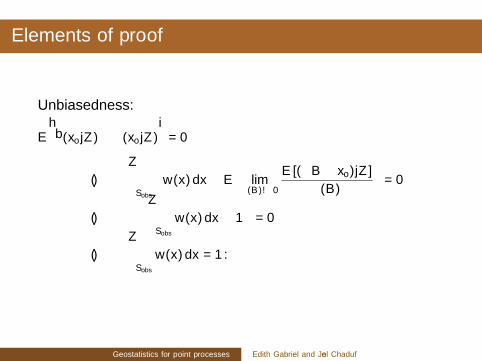
Unbiasedness:

E[λ(xo |Z )− λ(xo |Z )

]= 0

⇐⇒∫Sobs

λw(x) dx − E[

limν(B)→0

E [Φ(B ⊕ xo)|Z ]

ν(B)

]= 0

⇐⇒ λ

(∫Sobs

w(x) dx − 1

)= 0

⇐⇒∫Sobs

w(x) dx = 1.



Elements of proof

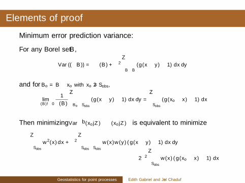
Minimum error prediction variance:

For any Borel set B,

Var (Φ(B)) = λν(B) + λ2∫B×B

(g(x − y)− 1) dx dy

and for Bo = B ⊕ xo with xo /∈ Sobs ,

limν(B)→0

1

ν(B)

∫Bo×Sobs

(g(x − y)− 1) dx dy =

∫Sobs

(g(xo − x)− 1) dx

Then minimizing Var(λ(xo |Z)− λ(xo |Z)

)is equivalent to minimize

λ

∫Sobs

w2(x) dx + λ2∫Sobs×Sobs

w(x)w(y) (g(x − y)− 1) dx dy

− 2λ2∫Sobs

w(x) (g(xo − x)− 1) dx



Elements of proof

Using Lagrange multipliers under the constraint on the weights, we set

T (w(x)) = λ

∫Sobs

w2(x) dx + λ2∫Sobs×Sobs

w(x)w(y) (g(x − y)− 1) dx dy

− 2λ2∫Sobs

w(x) (g(xo − x)− 1) dx + µ

(∫Sobs

w(x) dx = 1

)

Then, for α(x) = w(x) + ε(x),

T (α(x)) ≈ T (w(x)) + 2λ

∫Sobs

ε(x) [w(x)x + λw(y) (g(x − y)− 1) dy

−λ (g(x − o − x)− 1) +µ

2λ

]dx



Elements of proof

From variational calculation and the Riesz representation theorem,

T (α(x))− T (w(x)) = 0 ⇔∫Sobs

ε(x)

[w(x)x + λ

∫Sobs

w(y) (g(x − y)− 1) dy

− λ (g(xo − x)− 1) +µ

2λ

]dx = 0

⇔ w(x) + λ

∫Sobs

w(y) (g(x − y)− 1) dy

−λ (g(xo − x)− 1) +µ

2λ= 0

Thus,

1 + λ

∫S2obs

w(y) (g(x − y)− 1) dy dx − λ∫Sobs

(g(xo − x)− 1) dx +ν(Sobs)

2λµ = 0

from which we obtain µ and we can deduce the Fredholm equation

w(x)+λ

∫Sobs

w(y) (g(x − y)− 1) dy−1

ν(Sobs)

[1 +

∫S2obs

w(y) (g(x − y)− 1) dx dy

]

= λ (g(xo − x)− 1)−λ

ν(Sobs)

∫Sobs

(g(xo − x)− 1) dx



Solving the Fredholm equation

Any existing solution already considered in the literature can be used!

Our aim is to map the local intensity in a given window⇒ access to fast solutions.

Several approximations can be used to solve the Fredholm equation.

The weights w(x) can be defined as

step functions direct solution,

linear combination of known basis functions, e.g. splines

continuous approximation.

. . .

Here, we illustrate the ones with the less heavy calculations and implementation.



Step functions

Let consider the following partition of Sobs : Sobs = ∪nj=1Bj , with

B: elementary square centered at 0,Bj = B ⊕ cj : elementary square centered at cj ,Bk ∩ Bj = ∅,n: number of grid cell centers lying in Sobs .

For w(x) =∑n

j=1 wj

1{x∈Bj}ν(B) , we get λ(xo |Z ) =

∑nj=1 wj

Φ(Bj)

ν(B),

with w = (w1, . . . ,wn) = C−1Co + 1−1TC−1Co

1TC−11 C−11, where

C = λν(B)II + λ2ν2(B)(G − 1): covariance matrix

with G = {gij}i,j=1,...,n, gij = 1ν2(B)

∫B×B g(ci − cj + u − v) du dv ,

and II the n × n-identity matrix.

Co = λν(B)Ixo + λ2ν2(B)(Go − 1): covariance vector

with Ixo the n-vector with zero values and one term equals to one where xo = ci ,

and Go = {gio}i=1,...,n.



Step functions: variance of the predictor

We consider the Neuman series to invert the covariance matrix,C = λν(B)II + λ2ν2(B)(G − 1), when λν(B)→ 0:

C−1 =1

λν(B)[II + λν(B)Jλ] ,

where a generic element of the matrix Jλ is given by

Jλ[i , j] =∞∑k=1

(−1)kλk−1(g(xi , xl1 )− 1

) (g(xlk−1

, xj )− 1)

×∫Sk−1obs

k−2∏m=1

(g(xlm , xlm+1)− 1) dxl1 . . . dxlk−1

.

This leads to

Var(λ(xo |Z)

)= λ3ν2(B)(Go − 1)T (Go − 1) + λ4ν3(B)(Go − 1)T Jλ(Go − 1)

+1−

[λν(B)1T (Go − 1) + λ2ν2(B)1T Jλ(Go − 1)

]2

ν(Sobs )λ

+ ν2(B)1T Jλ1.



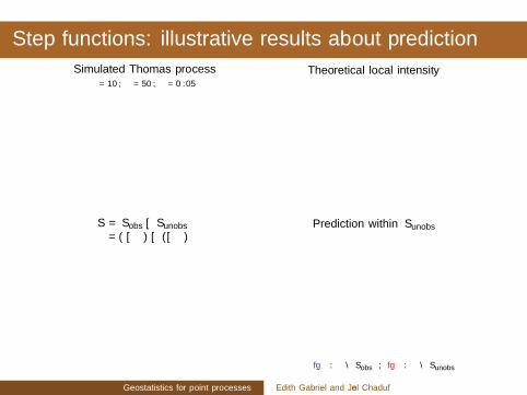
Step functions: illustrative results about prediction

Simulated Thomas processκ = 10, µ = 50, σ = 0.05

S = Sobs ∪ Sunobs= (∪��) ∪ (∪��)

Theoretical local intensity

Prediction within Sunobs

{•}: Φ ∩ Sobs ; {•}: Φ ∩ Sunobs



Spline basis

Let consider that the weights of λ(xo |Z ) =∑

x∈Φ∩Sobsw(x) are defined as

a degree d spline curve:

w(x) =k∑

i=1

hi,d(x),

where hi,d denotes the ith B-spline of order d .

A simplistic toy example in R:

Sobs = [0, L) ⊂ [0, L′] = S

Linear spline defined from equally-spaced knots xi :

w(x) =

a0 + b0x , x ∈ ∆0 = [x0, x1) = [0, L

k),

a1 + b1x , x ∈ ∆1 = [x1, x2) = [ Lk, 2L

k),

...

ak−1 + bk−1x , x ∈ ∆k−1 = [xk−1, xk ) = [ (k−1)Lk

, L),

= (ai + bi (x − xi )) 1{x∈∆i}



Spline basis

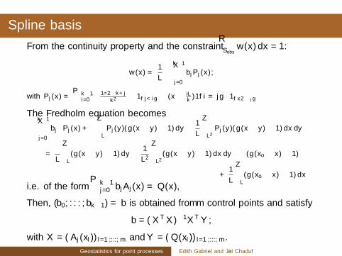
From the continuity property and the constraint∫Sobs

w(x) dx = 1:

w(x) =1

L−

k−1∑j=0

bjPj (x),

with Pj (x) =∑k−1

i=0

(1/2−k+j

k2 − 1{j<i} − (x − iLk

)1{i = j})

1{x∈∆i}

The Fredholm equation becomesk−1∑j=0

bj

[Pj (x) + λ

∫LPj (y)(g(x − y)− 1) dy −

1

L

∫L2

Pj (y)(g(x − y)− 1) dx dy

]

=λ

L

∫L(g(x − y)− 1) dy −

1

L2

∫L2

(g(x − y)− 1) dx dy − λ(g(xo − x)− 1)

+1

L

∫L(g(xo − x)− 1) dx

i.e. of the form∑k−1

j=0 bjAj(x) = Q(x),

Then, (b0, . . . , bk−1) = b is obtained from m control points and satisfy

b = (XTX )−1XTY ,

with X = (Aj(xl))l=1,...,m and Y = (Q(xl))l=1,...,m.



Spline basis: illustrative results

Thomas process in 1D (κ = 0.5, µ = 25, σ = 0.25)

0 5 10 15 20 25

0

20

40

60

x

loca

l int

ensi

ty

●●●●● ● ●● ●● ●● ●● ●● ●● ● ● ●● ●●● ●● ●●● ●●● ● ●● ●●●● ● ●● ● ●●● ●●●● ●● ●● ●● ●● ●●● ●● ●● ● ●● ●● ● ●●● ● ●● ● ●● ● ●● ●● ●● ●● ●●● ● ●● ●●●● ●●●●● ●●●●● ●● ●●● ● ●●● ●●● ● ●● ● ● ● ●● ●●●●●● ● ●● ● ●● ●●●● ●●● ●●● ●● ●● ●● ●● ●●●●● ●● ●●●●● ●● ● ●●●● ● ●● ● ●●● ●● ●● ● ●●● ●●● ● ●●●●●● ●●● ●●● ●● ●●●● ●●● ●● ●●●● ●● ●● ●●● ●● ●●● ●●●●● ●● ● ●● ●● ●●● ● ●●●●● ● ●●● ●●● ●● ●● ●● ● ● ● ●● ●●●●●●● ●● ● ●●● ●●●●●● ●●●●●● ● ●●● ● ●●●● ●●●● ● ● ●● ●●●●●●● ● ●● ●● ●● ●● ●● ●● ● ● ●● ●●● ●● ●●● ●●● ● ●● ●●●● ● ●● ● ●●● ●●●● ●● ●● ●● ●● ●●● ●● ●● ● ●● ●● ● ●●● ● ●●●● ●● ●●● ● ●●● ●●● ● ●● ● ● ● ●● ●●●●●● ● ●● ●●● ●● ● ●●●● ● ●● ● ●●● ●● ●● ● ●●● ●●● ● ●●●●●● ●●● ●●● ●● ●●●● ●●● ●● ●●●● ●● ●● ●●● ●● ●●● ●●●●● ●● ● ●● ●● ●●● ● ●●●●● ● ●●● ●●● ●● ●● ●●● ● ●● ●●●● ●●●● ● ●● ●●

0 5 10 15 20 25 30

0

20

40

60

80

x

loca

l int

ensi

ty● ●● ● ●●●●● ●●●●●●●● ●● ●●●● ●● ●●● ●●●● ●● ●●● ●●●●● ●● ●●● ●●●●●● ●● ●●●● ●● ● ●●●● ●● ● ●●●●● ●●● ●● ● ●●●●● ●●● ● ●●● ●●● ●●●● ●●● ●● ●●● ●●● ●●● ●●●● ●●● ● ●● ●●●●●●● ● ●●●● ●● ●● ●●●● ● ●● ● ●●● ●●●●● ●●● ●●●● ● ●●●●●● ● ●● ●● ●●● ●●●●●● ● ●●●● ●●●●●● ●● ●●● ●● ●●● ●●●●● ●●●● ●●● ● ●● ●● ●●● ●●● ●● ●●●● ● ●● ●● ●● ●●● ●●●● ● ●●●● ●● ●●● ●●● ● ●●●●●● ●●● ●●●● ●● ● ●●●● ●● ●●●●● ●● ●●● ●● ● ●● ● ●●●● ●●● ● ●● ● ● ●● ●●● ●● ●●●● ●● ●●● ●●●●● ●● ●●● ● ● ●●● ●● ● ●● ●●● ●●● ● ●● ●●● ●●● ● ●● ●● ●●●●● ●● ●● ●● ●●●● ●●●● ●●●●●● ●●● ● ● ● ●●● ●●●●● ●●●●● ●● ● ●●● ●●●●● ●●●●● ● ●● ●●● ●●●● ●● ●● ●● ● ●●●●● ●●● ● ●● ●●● ●●● ● ●● ●●● ●● ●● ●●●●● ●●● ●●● ●●● ●● ● ●●● ●● ●●●●● ●●●● ●●●●●●● ●●●●●●●● ●● ●●● ●● ●●●● ●●● ●● ●● ●●●● ●●●●●●● ● ●●●● ●●● ●●●● ●●●●● ●●●● ●● ●●●●● ●● ●●● ●●●●● ●● ●●● ●●●●●● ●● ●● ● ●●●●● ●●● ● ●●● ●●● ●●●● ●●● ●● ●●● ●●● ●●● ●●●● ●●● ● ●● ●●●●●●● ● ●●●● ●● ●● ●●●● ● ●●●● ● ●● ●● ●●● ●●●●●● ● ●●●● ●●●●●● ●● ●●● ●● ●●● ●●●●● ●●●● ●●● ● ●● ●● ●●● ●●● ●● ●●●● ● ●● ●● ●● ●●● ●●●● ●● ● ●●●● ●● ●●●●● ●● ●●● ●● ● ●● ● ●●●●● ●●●● ●● ●●● ●●●●● ●● ●●● ● ● ●●● ●● ● ●● ●●● ●●● ● ●● ●●● ●●● ● ●● ●● ●●●●● ●● ●● ●● ●●●● ●●●● ●●●●●● ●●● ● ● ● ●●● ●●●●● ●●●●● ●● ● ●●● ●●●●● ●●●●● ● ●● ●●● ●●●● ●● ●● ●● ● ●●●●● ●●● ● ●● ●●● ●●● ●●● ●●●●● ●● ●●● ●● ●●●● ●●● ●● ●● ●●●● ●●●●●●● ● ●●●● ●●● ●●●● ●●●●● ●●●● ●● ●●

−−−− Theoretical local intensity on Sobs ; −−−− Predicted values ; −− Intensity of Φ

{•} = ΦSobs ; {•} = ΦSunobs



In practice: g must be estimated

Simulated Thomas processκ = 10, µ = 50, σ = 0.05

Estimated pcf

Prediction within Sunobs(with the theoretical pcf)

R2 = 0.85

(with the estimated pcf)

R2 = 0.8

R2 in linear regressionof predicted and theoretical values

(with the theoretical pcf)

(with the estimated pcf)

{•}: Φ ∩ Sobs ; {•}: Φ ∩ Sunobs



In practice

Application to Montagu’s Harriers’ nest locations

Data collection

Estimated pcf Prediction

● ●●●

●

●

●

● ●

●●●

●

●

●

●

●

●●

●

●●

● ●

●

●

●

●●●

●

●

●

●

●

●

●

●

●

●

●●

●●

●

●

●

●

●

●●

●

●

●

●

●

●

●

●

●

●

●

●

●

●

●●

●

●

●

●

●

●●

●

●

●

●

●

●

●

●

●

●

● ●

●

●

●

●

●

●

●

●

●

●

●

●

●

●

●

●

●

● ●

●

●

●

●

●

●

●●

●

●●

●

●

●●

●

●

●

●

●●●●●

●●

●

●

●●

●

●

●

●

● ●

●

●

●

●

●

●

●

●

●

●

●●

●

●

●

●●

●● ●

●●

●●

●●

●

●

●

●

●

●

●

●●

●●

●●

●●●

●

●

●

●

●

●

●

●

●

●

●

●

●

●●

●

●

●

●

●

●

●

●●

●

●

●

●

●

● ●

●

●

●●●

●●

●

●

●

●●

●

●

●

● ●●

●

● ●

●●

●

●

●

● ●●

●

●

●

●

●

●

●

●

●

●●

●

●

●

●

●

●●

●

●

●

●

●

●

●

●

●

●

●

●

●

●

●

●

●

●

●

●

●●

●

●

●●

●

● ●

●

●

●

●

●

●

●

●

●

●●●

●●●

●

●

●

●

●

●●●

● ●

●

●

●

●

●

●

●

●●

●●

●● ●●●

●

●●

●

●

●

●

●●

●

●●

●

●● ●

●

●

●

●

●

●

●

●

●

●

●●

●

●

●●

●

● ●

●

●●

●

●

●●

●

●●●

●●

●

●●

●

●

●

●

●

●

●

●

●

●

●

●

●

●

●

●

●

●

●

●

{•} = ΦSobs; {•} = ΦSunobs



Work in progress

Take into account some covariates in the prediction.

Get results with splines on the plane.

Use finite elements method to solve the Fredholm equation.

Determine the properties of the related predictor.

Extend the approach to the spatio-temporal setting.



References

E. Bellier et al. (2013) Reducting the uncertainty of wildlife population abundance:model-based versus design-based estimates. Environmetrics, 24(7):476–488.

E. Gabriel et al. (2016) Adapted kriging to predict the intensity of partially observedpoint process data. Spatial statistics, in revision.

P. Diggle and P. Ribeiro (2007) Model-based geostatistics. Springer.

P. Diggle et al. (2013) Spatial and spatio-temporal log-gaussian cox processes:extending the geostatistical paradigm. Statistical Science, 28(4):542–563.

P. Monestiez et al. (2006) Geostatistical modelling of spatial distribution ofbalaenoptera physalus in the northwestern mediterranean sea from sparse count dataand heterogeneous observation efforts, Ecological Modelling, 193:615–628.

A. Tscheschel and D. Stoyan (2006) Statistical reconstruction of random pointpatterns. Computational Statistics and Data Analysis, 51:859–871.


geostatistics for point processes - lebesgue

Documents