getting started in r for biologists - university of hawaiimbutler/rquickstart/simpler.pdfgetting...
TRANSCRIPT
Getting Started in R for Biologists
Marguerite A. Butler1,2
1Department of Zoology, University of Hawaii, Honolulu, HI [email protected]
January 4, 2009

2

Contents
1 Preliminaries 5
1.1 Computer Requirements and Installing R . . . . . . . . . . . . . . . . . . 5
1.1.1 Installing from source . . . . . . . . . . . . . . . . . . . . . . . . . 5
1.2 R packages . . . . . . . . . . . . . . . . . . . . . . . . . . . . . . . . . . . 6
1.3 Comparative Methods in R References . . . . . . . . . . . . . . . . . . . 7
1.4 General R References . . . . . . . . . . . . . . . . . . . . . . . . . . . . . 7
1.5 General Comparative Methods References . . . . . . . . . . . . . . . . . 7
1.6 Help! and Useful References . . . . . . . . . . . . . . . . . . . . . . . . . 7
1.6.1 general R help . . . . . . . . . . . . . . . . . . . . . . . . . . . . . 7
1.6.2 comparative methods R help . . . . . . . . . . . . . . . . . . . . . 8
2 Playing with R for the first time 9
2.1 Instructions . . . . . . . . . . . . . . . . . . . . . . . . . . . . . . . . . . 9
2.2 R session . . . . . . . . . . . . . . . . . . . . . . . . . . . . . . . . . . . . 9
2.3 Insert Comments . . . . . . . . . . . . . . . . . . . . . . . . . . . . . . . 10
3 Finding Help 13
3.1 When you know the name of the function . . . . . . . . . . . . . . . . . . 13
3.2 Don’t know the name of the function . . . . . . . . . . . . . . . . . . . . 14
3.3 Package-specific help . . . . . . . . . . . . . . . . . . . . . . . . . . . . . 15
4 Creating Data Objects and Plotting 17
4.1 Data objects . . . . . . . . . . . . . . . . . . . . . . . . . . . . . . . . . . 17
3
4 CONTENTS
4.2 Simple plotting . . . . . . . . . . . . . . . . . . . . . . . . . . . . . . . . 20
4.2.1 Bivariate plot . . . . . . . . . . . . . . . . . . . . . . . . . . . . . 20
4.2.2 Univariate plot . . . . . . . . . . . . . . . . . . . . . . . . . . . . 21
5 What is it? 25
6 Data Input and Output 29
6.1 Getting your data into R . . . . . . . . . . . . . . . . . . . . . . . . . . . 29
6.1.1 read.csv . . . . . . . . . . . . . . . . . . . . . . . . . . . . . . . . 29
6.2 Summary statistics on your data . . . . . . . . . . . . . . . . . . . . . . . 31
6.2.1 merge . . . . . . . . . . . . . . . . . . . . . . . . . . . . . . . . . 32
6.3 write.csv . . . . . . . . . . . . . . . . . . . . . . . . . . . . . . . . . . . . 33
6.4 save . . . . . . . . . . . . . . . . . . . . . . . . . . . . . . . . . . . . . . 33
6.5 Saving plots . . . . . . . . . . . . . . . . . . . . . . . . . . . . . . . . . . 34
6.5.1 pdf . . . . . . . . . . . . . . . . . . . . . . . . . . . . . . . . . . . 36
6.6 Messier input files . . . . . . . . . . . . . . . . . . . . . . . . . . . . . . . 37
6.6.1 Input files generated by data loggers . . . . . . . . . . . . . . . . 37
7 The Workhorse Functions of Data Manipulation 41
7.1 Indexing and subsetting . . . . . . . . . . . . . . . . . . . . . . . . . . . 41
7.2 String Matching . . . . . . . . . . . . . . . . . . . . . . . . . . . . . . . . 44
7.3 Ordering Data . . . . . . . . . . . . . . . . . . . . . . . . . . . . . . . . . 45
7.4 Matching . . . . . . . . . . . . . . . . . . . . . . . . . . . . . . . . . . . 47
7.5 Merging . . . . . . . . . . . . . . . . . . . . . . . . . . . . . . . . . . . . 50
7.6 Reshaping R Objects . . . . . . . . . . . . . . . . . . . . . . . . . . . . . 51
8 Answers to Exercises – Creating Data Objects 55
9 Answers to Exercises – The Workhorse Functions of Data Manipulation 65
Chapter 1
Preliminaries
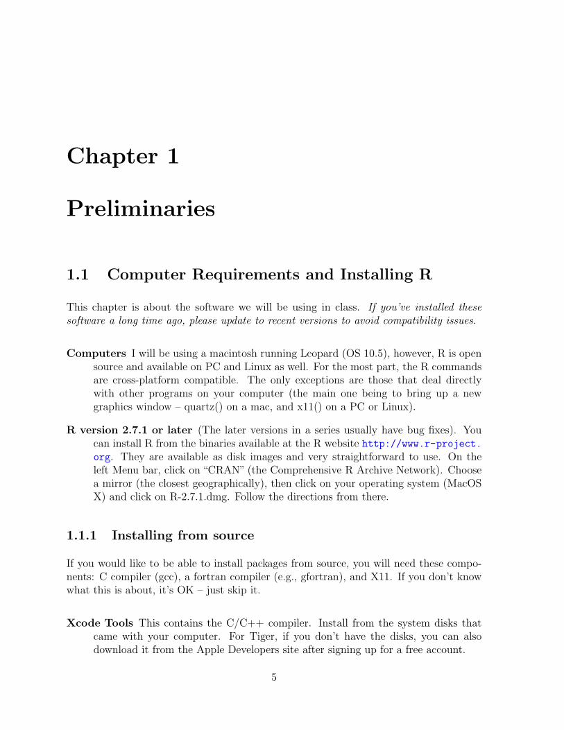
1.1 Computer Requirements and Installing R
This chapter is about the software we will be using in class. If you’ve installed thesesoftware a long time ago, please update to recent versions to avoid compatibility issues.
Computers I will be using a macintosh running Leopard (OS 10.5), however, R is opensource and available on PC and Linux as well. For the most part, the R commandsare cross-platform compatible. The only exceptions are those that deal directlywith other programs on your computer (the main one being to bring up a newgraphics window – quartz() on a mac, and x11() on a PC or Linux).
R version 2.7.1 or later (The later versions in a series usually have bug fixes). Youcan install R from the binaries available at the R website http://www.r-project.
org. They are available as disk images and very straightforward to use. On theleft Menu bar, click on “CRAN” (the Comprehensive R Archive Network). Choosea mirror (the closest geographically), then click on your operating system (MacOSX) and click on R-2.7.1.dmg. Follow the directions from there.
1.1.1 Installing from source
If you would like to be able to install packages from source, you will need these compo-nents: C compiler (gcc), a fortran compiler (e.g., gfortran), and X11. If you don’t knowwhat this is about, it’s OK – just skip it.
Xcode Tools This contains the C/C++ compiler. Install from the system disks thatcame with your computer. For Tiger, if you don’t have the disks, you can alsodownload it from the Apple Developers site after signing up for a free account.
5
6 CHAPTER 1. PRELIMINARIES
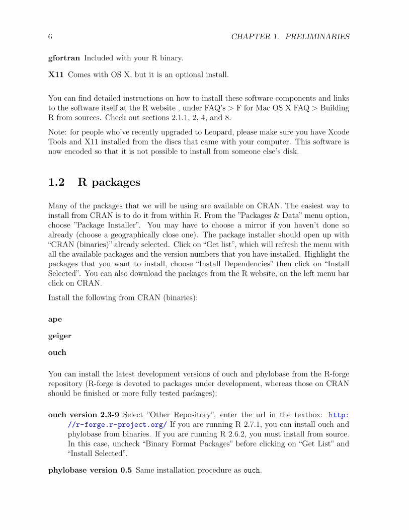
gfortran Included with your R binary.
X11 Comes with OS X, but it is an optional install.
You can find detailed instructions on how to install these software components and linksto the software itself at the R website , under FAQ’s > F for Mac OS X FAQ > BuildingR from sources. Check out sections 2.1.1, 2, 4, and 8.
Note: for people who’ve recently upgraded to Leopard, please make sure you have XcodeTools and X11 installed from the discs that came with your computer. This software isnow encoded so that it is not possible to install from someone else’s disk.
1.2 R packages
Many of the packages that we will be using are available on CRAN. The easiest way toinstall from CRAN is to do it from within R. From the ”Packages & Data” menu option,choose ”Package Installer”. You may have to choose a mirror if you haven’t done soalready (choose a geographically close one). The package installer should open up with“CRAN (binaries)” already selected. Click on “Get list”, which will refresh the menu withall the available packages and the version numbers that you have installed. Highlight thepackages that you want to install, choose “Install Dependencies” then click on “InstallSelected”. You can also download the packages from the R website, on the left menu barclick on CRAN.
Install the following from CRAN (binaries):
ape
geiger
ouch
You can install the latest development versions of ouch and phylobase from the R-forgerepository (R-forge is devoted to packages under development, whereas those on CRANshould be finished or more fully tested packages):
ouch version 2.3-9 Select ”Other Repository”, enter the url in the textbox: http:
//r-forge.r-project.org/ If you are running R 2.7.1, you can install ouch andphylobase from binaries. If you are running R 2.6.2, you must install from source.In this case, uncheck “Binary Format Packages” before clicking on “Get List” and“Install Selected”.
phylobase version 0.5 Same installation procedure as ouch.
1.3. COMPARATIVE METHODS IN R REFERENCES 7
1.3 Comparative Methods in R References
Phylogenetic Comparative Methods Wiki Tutorials and overview of methods avail-able in R for phylogenetic comparative analysis. The wiki grew out of a Hackathonon Comparative Methods in R held at the National Evolutionary Synthesis Center(NESCent) 10-14 December 2007.
Analysis of Phylogenetics and Evolution with R A book written by ?. This bookis a very useful reference on how to do evolutionary analyses using the ape package,written by one its developers. It is available from Springer and Amazon.
1.4 General R References
An introduction to R A comprehensive and easy-to-follow tutorial produced by theR Development Core Team.
R for Beginners A tutorial by Emmanuel Paradis.
1.5 General Comparative Methods References
The Comparative Method in Evolutionary Biology An book written by ?. It isgetting a bit old now, but it is still a comprehensive general reference and a usefuloverview of many methods.
Phylogenies and the Comparative Method in Animal Behavior A volume editedby ?, with explanation of methods and nice examples. Available at books.google.comfor preview.
Inferring Phylogenies Joe Felsenstein’s (?) book. It is mostly about phylogeny recon-struction, but there is a chapter on comparative methods that gives Felsenstein’sperspective on comparative analysis.
1.6 Help! and Useful References
1.6.1 general R help
Jonathan Baron’s R help page Bookmark this page! It is the best search engine tofind R help. It searches the huge archives of the R-help listserv as well as all Rdocumentation pages. For more technical help, you can also include the R-dev(developers) listserv in the search.

8 CHAPTER 1. PRELIMINARIES
1 page R reference card by Jonathan Baron.
4 page R reference card by Tom Short.
1.6.2 comparative methods R help
R-sig-phylo mailing list The listserv for the R Phylogenetic Comparative MethodSpecial Interest Group. It is archived here.
Chapter 2
Playing with R for the first time
2.1 Instructions
In this exercise, I want to introduce you to some of the built-in help facilities and docu-mentation in R, and get you started with manipulating variables in R.
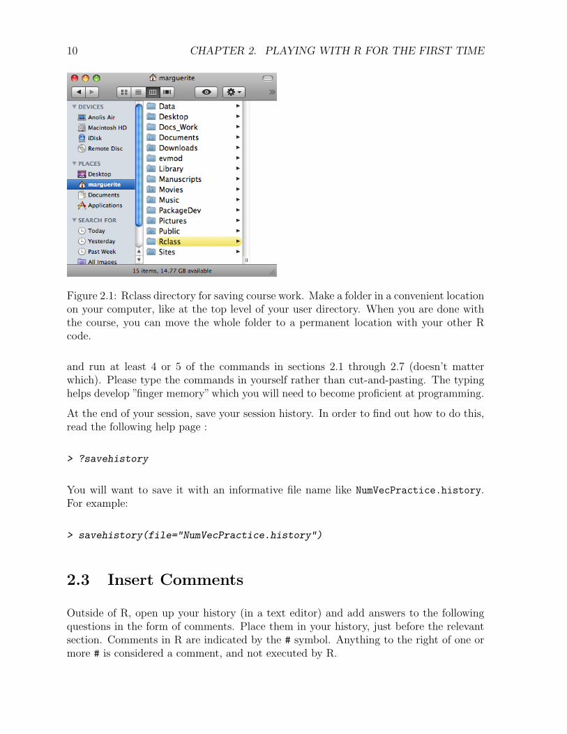
• If you haven’t already done so, make a directory for this class. I would recommendnaming it “Rclass” and putting it at some accessible location in your user directory(like at the top level of your User directory on a Mac, or at C:/ on a windowsmachine). On my computer it would be (Fig. 2.1):
• Start up R.
• Move to your Rclass directory by using the setwd("path to Rclass ") command.
> setwd("~/Rclass")
On a PC it will be something like:
> setwd("C:/Rclass")
• Open the help facility using the command
> help.start()
• Click on ”An Introduction to R”. The is ”the Bible” for learning R.
2.2 R session
Later, when you have more time, you will want to read and try out all of the section”Simple manipulations; numbers and vectors” (2.1 – 2.8). For now, take about 10 minutes
9
10 CHAPTER 2. PLAYING WITH R FOR THE FIRST TIME
Figure 2.1: Rclass directory for saving course work. Make a folder in a convenient locationon your computer, like at the top level of your user directory. When you are done withthe course, you can move the whole folder to a permanent location with your other Rcode.
and run at least 4 or 5 of the commands in sections 2.1 through 2.7 (doesn’t matterwhich). Please type the commands in yourself rather than cut-and-pasting. The typinghelps develop ”finger memory” which you will need to become proficient at programming.
At the end of your session, save your session history. In order to find out how to do this,read the following help page :
> ?savehistory
You will want to save it with an informative file name like NumVecPractice.history.For example:
> savehistory(file="NumVecPractice.history")
2.3 Insert Comments
Outside of R, open up your history (in a text editor) and add answers to the followingquestions in the form of comments. Place them in your history, just before the relevantsection. Comments in R are indicated by the # symbol. Anything to the right of one ormore # is considered a comment, and not executed by R.

2.3. INSERT COMMENTS 11
1. What is a numeric vector?Answer: ## A numeric vector is an ordered collection of numbers.
2. Is ordinary arithmetic (+, -, *, /) on vectors in R done element-by-element or usingmatrix math? (to test an example, try or think about x*y where:
x =
(12
)y =
(51
)3. What is a sequence?
4. What is an logical value? What is a logical vector?
5. What is a missing value?
6. What is a character vector?
7. What is an index vector?

12 CHAPTER 2. PLAYING WITH R FOR THE FIRST TIME
Chapter 3
Finding Help
R has great built-in help facilities. Once you get used to R’s syntax (the form of Rfunctions and data), you will find them incredibly useful.
Every object that comes with the R program is documented in some way – this meansevery function, internal dataset, as well as methods and classes (which we won’t havetime to cover).
3.1 When you know the name of the function
Say you want to find the mean of your data, so you guess that there is a function calledmean(). Finding help is easy:
> ?mean
Will bring up the help page, and is equivalent to:
> help(mean)
Notice that as you type help( you start to see the function definition on the bottom ofthe console window. It shows you how to call the function (what variables it expects).
Looking at the help page, notice that there are sections (these are common to most helppages):
Description what it does
Usage the format for calling the function (making it run)
13

14 CHAPTER 3. FINDING HELP
Arguments explanation for each of the arguments, their type, and what they represent
Details more explanation
Value what is returned from calling the function
Author
References
See Also other functions to check out
Examples Often the most valuable section, with examples that actually work. You cantest them out by cutting and pasting into the R console.
There are also hyperlinks in many help documents, to related help pages, so you can“surf” you way through help.
3.2 Don’t know the name of the function
But first to access the help for a specific function, you need to know what it is called.
Two good options are:
> help.start()
Which will bring up an an html browser, which you can browse. Click on “Packages”,then “base” if you are looking for a basic function that should be in the base distributionof R. Click on the package name if you are looking for a function in a package. Browsingthrough the help is very useful for beginners.
> help.search("plot")
Will do a “fuzzy” search (i.e., will also match words close in spelling – not exact – toplot). Of course, replace ”plot” with whatever you are looking for. This function searchesthrough the full text of the help docs, so for a common word like plot, this will return ahuge list, which you can look through package by package.
3.3. PACKAGE-SPECIFIC HELP 15
3.3 Package-specific help
Packages are generally a set of functions that are loaded from some (hidden) directoryon your computer into active memory, so that you can use them by name. Now that youknow the names of the functions, you can access specific help pages directly. Try the helppage for independent contrasts:
> help(pic)
Here’s a harder example. you might want to know more about the phylogeny plottingfunction in ape. If tree is a tree object in ape, you can useplot(tree) to call thefunction, so you might think that you can find the help page by using help(plot) or?plot. However, this brings up the generic plot function which doesn’t say anythingabout the one you want (the tree plotting function in ape.
What is going on is that ape has a method set for plotting objects of the class phylo,so that you don’t have to remember the specific function name. This is actually awonderful feature of object-oriented programming, otherwise you would have to rememberthousands of functions, all uniquely named.
So how do we find the one we want? You could try:
> help(plot, package="ape")
But you will see that this doesn’t return anything. This means that the actual plottingfunction in ape is named something else, so that there is no function in ape named ”plot”(R requires all named functions in packages to be documented).
Huh? How does plot() plot a phylogenetic tree when there is no function called plot inape? This is an example of a generic function. The function plot is actually a generic,with different specific functions for different types of objects – R automatically choosesthe correct one by looking at the objects class.
Anyway...
You have a couple more options (in addition to the general options above):
help(package=“ape”) will return the package’s main help page, where you can seea list of functions, but they are not clickable. Once you locate the name of thefunction you can follow up with a help(plot.phylo).
methods(plot) will return all of the methods written for the generic plot call. Lookingthrough it, you might guess that plot.phylo is the one you want. NOTE: thisonly works for S3 methods.

16 CHAPTER 3. FINDING HELP
Chapter 4
Creating Data Objects and Plotting
4.1 Data objects
Now that you have been introduced to R’s data objects, we’ll practice creating them. Rhas a rich collection of functions which are very helpful for creating and manipulatingobjects, so a bit of code can substitute for whole lot of typing!
The tables below list some helpful functions. Look up help for anything you don’t know.It will soon start making sense!
commands actionsc(n1, n2, n3) combines elements into an objectcbind(x, y) binds objects together by columnrbind(x, y) binds objects together by row
Table 4.1: Common combine functions used for creating data objects from existing objects
commands actionsseq() generate a sequence of numbers1:10 sequence from 1 to 10 by 1rep(x, times) replicates xsample(x, size, replace=FALSE) sample size elements from xrnorm(n, mean=0, sd=1) draw n samples from normal distribution
Table 4.2: Functions used for creating sequences and sampling
Factors are categorical data, for example, “large” and “small”, or “blue”, “red”’, and “yel-low”. Factors may be ordered, which means that the order of the categories has meaning(like size categories). By default, factors are unordered. Levels are the values (i.e., namesof the categories) that the factor can take.
17
18 CHAPTER 4. CREATING DATA OBJECTS AND PLOTTING
commands actionsvector() create a vectormatrix() create a matrixdata.frame() create a data.frameas.vector(x) coerces x to vectoras.matrix(x) coerces to matrixas.data.frame(x) coerces to data frameas.character(x) coerces to characteras.numeric(x) coerces to numericfactor(x) creates factor levels for elements of xlevels() orders the factor levels as specified
Table 4.3: Functions used for creating and coercing objects to new type/class
Examples
To get you started, here are some examples. Creating vectors:
> x <- c( 1, 5, 7, 14)
> x
[1] 1 5 7 14
> x <- rep( x, times=2)
> x
[1] 1 5 7 14 1 5 7 14
> y <- rnorm(8)
> y
[1] -0.5693700 1.8304079 -1.4685032 0.7484051 1.1500837 -0.8391118 1.4191586
[8] 0.5397137
> species <- letters[1:4] # special stored data object: lower case letters a - d
> species
[1] "a" "b" "c" "d"
> LETTERS[1:3] # A B C

4.1. DATA OBJECTS 19
[1] "A" "B" "C"
> treatment <- c("high", "med", "low")
> treat <- factor(treatment) # create a factor
> treat
[1] high med low
Levels: high low med
> as.numeric(treat) # coerce to numeric
[1] 1 3 2
> x <- factor(x) # factor
Notice that your work is only saved if you STORE the result in an obect
Creating a matrix:
> xy <- cbind(x,y) # column bind
> xy
x y
[1,] 1 -0.5693700
[2,] 2 1.8304079
[3,] 3 -1.4685032
[4,] 4 0.7484051
[5,] 1 1.1500837
[6,] 2 -0.8391118
[7,] 3 1.4191586
[8,] 4 0.5397137
> z <- matrix(1:25, nrow=5) #create a matrix with 5 rows
> z
[,1] [,2] [,3] [,4] [,5]
[1,] 1 6 11 16 21
[2,] 2 7 12 17 22
[3,] 3 8 13 18 23
[4,] 4 9 14 19 24
[5,] 5 10 15 20 25
Creating a data matrix:
> dat <- data.frame(species, x, y)

20 CHAPTER 4. CREATING DATA OBJECTS AND PLOTTING
4.2 Simple plotting
The generic function for plotting in R is plot.
4.2.1 Bivariate plot
When you supply two vectors to plot, is assumes that the first one is the X coordinate, andthe second is the Y. If the first object is a continuous variable, you will get a scatterplot.
> plot(y,x) # continuous variable first - plots as a scatterplot
●
●
●
●
●
●
●
●
−1.5 −1.0 −0.5 0.0 0.5 1.0 1.5
1.0
1.5
2.0
2.5
3.0
3.5
4.0
y
x
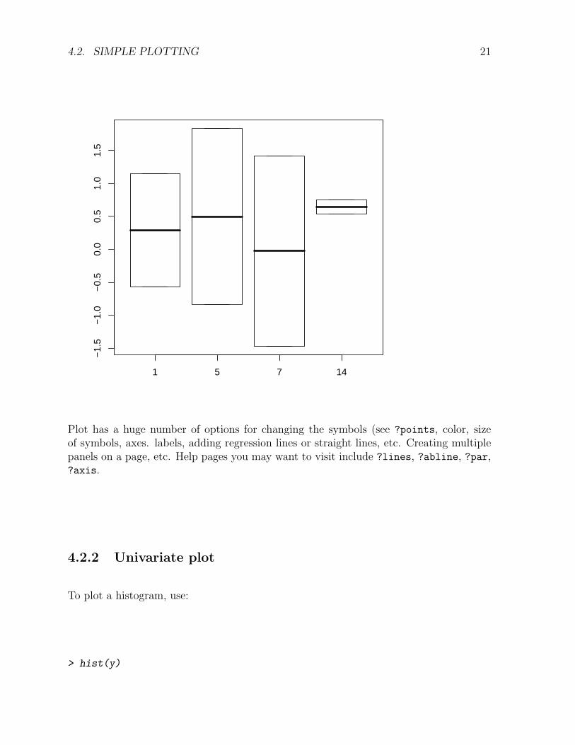
However, if the firstobject is a factor, you will get a boxplot.
> plot(x, y) # categorical variable first - plots as a boxplot
4.2. SIMPLE PLOTTING 21
1 5 7 14
−1.
5−
1.0
−0.
50.
00.
51.
01.
5
Plot has a huge number of options for changing the symbols (see ?points, color, sizeof symbols, axes. labels, adding regression lines or straight lines, etc. Creating multiplepanels on a page, etc. Help pages you may want to visit include ?lines, ?abline, ?par,?axis.
4.2.2 Univariate plot
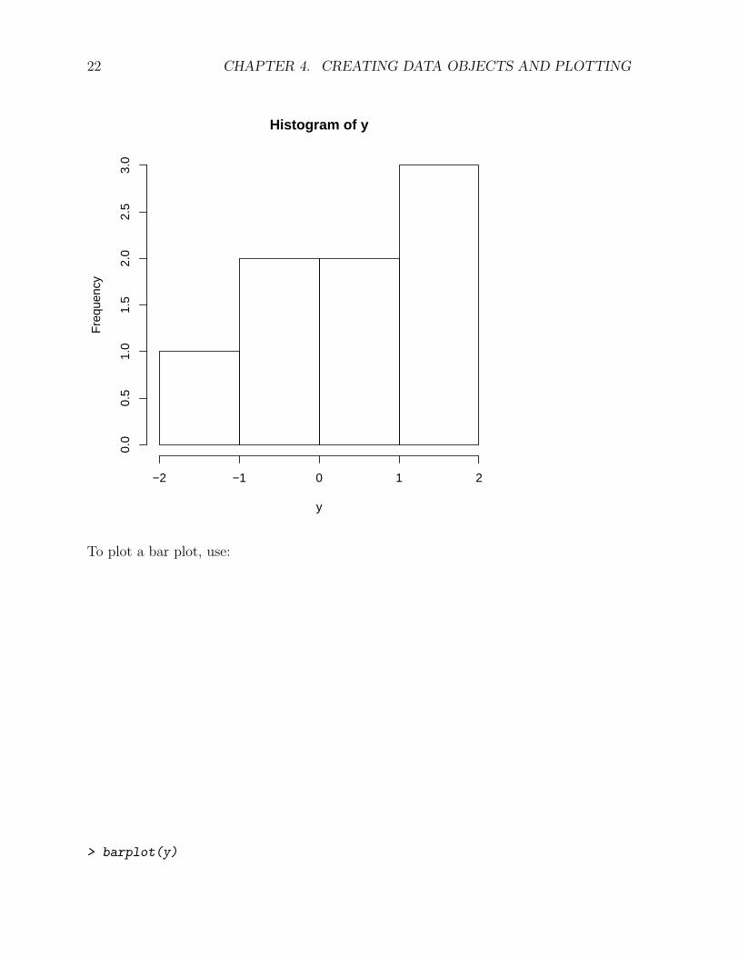
To plot a histogram, use:
> hist(y)
22 CHAPTER 4. CREATING DATA OBJECTS AND PLOTTING
Histogram of y
y
Fre
quen
cy
−2 −1 0 1 2
0.0
0.5
1.0
1.5
2.0
2.5
3.0
To plot a bar plot, use:
> barplot(y)

4.2. SIMPLE PLOTTING 23
−1.
0−
0.5
0.0
0.5
1.0
1.5
Practice
1. Create a dataset with simulated data using rnorm().
(a) Simulate 21 random data points drawn from a normal distribution (create anumeric vector), and save it in the variable “y”. Create a second set of 21points and save it as “y1”.
> y <- rnorm(21)
> y1 <- rnorm(21)
> y
[1] -0.11186058 -1.21675753 0.57724121 1.07825545 -0.64108807 -1.62443215
[7] 1.16993567 1.84654085 -0.72732573 0.98336334 0.05906814 -0.82409271
[13] -0.37663569 1.11170131 -0.87463772 0.61278171 0.60031860 -0.21237995
[19] -1.86681684 1.10421075 1.75443152
> y1

24 CHAPTER 4. CREATING DATA OBJECTS AND PLOTTING
[1] -0.58574022 -0.08278102 1.53222267 0.56692497 -0.18830992 0.17758962
[7] 0.65121116 -0.30428366 0.75080530 -0.47102748 1.60921356 -0.72107953
[13] -0.54004728 1.87995286 -0.38419521 0.38956171 0.15907504 -2.34570497
[19] -2.13285350 2.20112661 -1.50941706
(b) Create a treatment vector with levels “low”, “med”, and “high”, save it as afactor.
> treatment <- factor( c("low", "med", "high") )
> treatment
[1] low med high
Levels: high low med
(c) Our treatment has numeric values also, so create a numeric vector with thevalues 2, 4, 8, save it as x.
(d) Create a species vector with seven names.
(e) Create a matrix with y in the first column and x in the second column, saveit as dat.matrix.
(f) Create a data frame with species, x, treatment, y and y1, save as dat. Whycan’t you make a matrix with these columns?
(g) Make a bivariate plot of the numeric value of the treatment (x) versus theresponse (y). You may want to check the help documentation for ”plot”. Youwill have to select the columns of the data frame.
(h) Make a plot on the treatment as factor versus the response. What is thedifference between these two plots?
(i) Is the factor displayed in the plot in the order that makes sense? If not, fixthis by applying factor to the treatment column of dat again, but this timespecifying the levels vector with names of the levels in the order you want.You may want to look at the help page for factor. Plot it again.
(j) Let’s make a scatterplot (plot(y, y1)) to see if there is any structuring in thedata (eventually with respect to the treatment levels – the rest of this exerciseis in the chapter on Workhorse Functions of Data Analysis). While we’re atit, let’s make it prettier. Change the symbols to solid circles by adding theoptional parameter pch=16, and the points bigger by cex=2. Change the colorto red using col="red".
(k) Now let’s make some data which should differ. For the ”low” treatment, sim-ulate y and y1 as normally distributed data with mean = -2 and sd=.5, and”high” as mean=5, and sd=3. Remake the dataframe.
(l) Now make two boxplots: treatment vs. y and treatment vs. y1.
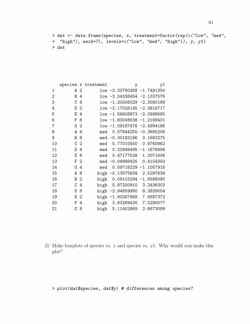
(m) Make boxplots of species vs. y and species vs. y1. Why would you make thisplot?

Chapter 5
What is it?
When working with a new package, you want to know what kind of object you are dealingwith. Check its class and attributes.
To illustrate, let’s make up some data:
> x <- 1:9
> x
[1] 1 2 3 4 5 6 7 8 9
> class(x)
[1] "integer"
x is a numeric vector. Vectors have length, but not dimension:
> length(x)
[1] 9
> dim(x)
NULL
However, we can easily change it into a matrix by giving it row and column dimensions.This has to be specified as a vector with number of rows, number of columns, here madewith the combine function: c(3,3)
25
26 CHAPTER 5. WHAT IS IT?
> dim(x) <- c(3,3)
> x
[,1] [,2] [,3]
[1,] 1 4 7
[2,] 2 5 8
[3,] 3 6 9
> class(x)
[1] "matrix"
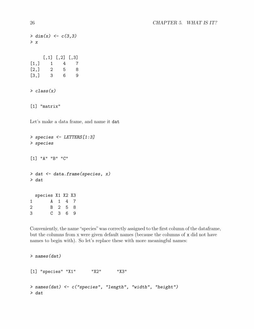
Let’s make a data frame, and name it dat
> species <- LETTERS[1:3]
> species
[1] "A" "B" "C"
> dat <- data.frame(species, x)
> dat
species X1 X2 X3
1 A 1 4 7
2 B 2 5 8
3 C 3 6 9
Conveniently, the name“species”was correctly assigned to the first column of the dataframe,but the columns from x were given default names (because the columns of x did not havenames to begin with). So let’s replace these with more meaningful names:
> names(dat)
[1] "species" "X1" "X2" "X3"
> names(dat) <- c("species", "length", "width", "height")
> dat
27
species length width height
1 A 1 4 7
2 B 2 5 8
3 C 3 6 9
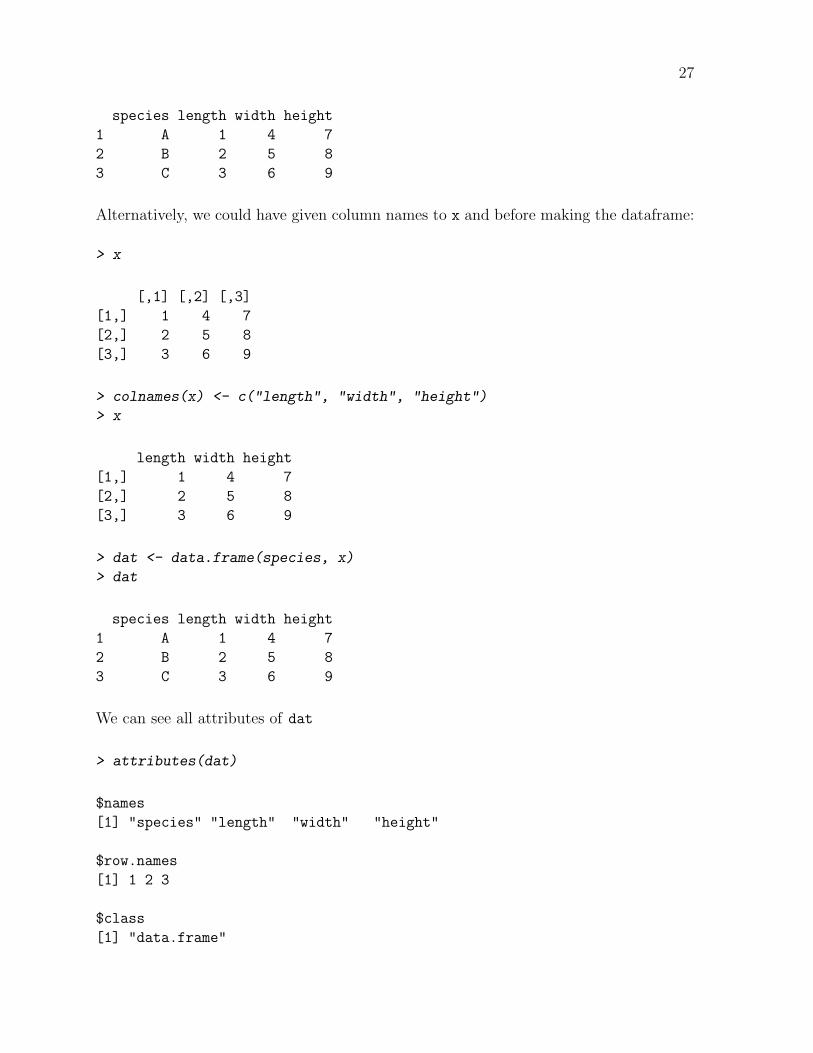
Alternatively, we could have given column names to x and before making the dataframe:
> x
[,1] [,2] [,3]
[1,] 1 4 7
[2,] 2 5 8
[3,] 3 6 9
> colnames(x) <- c("length", "width", "height")
> x
length width height
[1,] 1 4 7
[2,] 2 5 8
[3,] 3 6 9
> dat <- data.frame(species, x)
> dat
species length width height
1 A 1 4 7
2 B 2 5 8
3 C 3 6 9
We can see all attributes of dat
> attributes(dat)
$names
[1] "species" "length" "width" "height"
$row.names
[1] 1 2 3
$class
[1] "data.frame"

28 CHAPTER 5. WHAT IS IT?
A vector has no dimension. So it’s easy to turn x from a matrix back to a vector bygetting rid of its dimensions. NULL is a special R variable.
> dim(x) <- NULL
> x
[1] 1 2 3 4 5 6 7 8 9
> class(x)
[1] "integer"
Another useful ”What is it” function is str for structure, which nicely summarizes whatit is:
> str(dat)
'data.frame': 3 obs. of 4 variables:
$ species: Factor w/ 3 levels "A","B","C": 1 2 3
$ length : int 1 2 3
$ width : int 4 5 6
$ height : int 7 8 9

Chapter 6
Data Input and Output
So far, we have been working within R, either typing data in directly or using R’s functionsto generate data. In order to analyze your own data, you have to load data from anexternal file into R. Similarly, to save your work, you’ll probably want to write files fromR to your hard drive. Both of these require interacting with your computer’s operatingsystem. In this chapter, we’re just going to do it. We’ll talk more about what’s going onin a later section on the R Environment.
6.1 Getting your data into R
The most convenient way to read data into R is using the read.csv() function. Thisrequires that your data is saved in .csv format, which is possible from Microsoft Excel(save as... csv) or any spreadsheet format. It is a text format with data separated bycommas. It is very nice because it is unambiguous, not easily corruptible, and non-proprietary. Thus it is readable by nearly every program that reads in data.
First, within your “Rclass” folder, create a folder named“Data”. Copy the file “anolis.csv”and “Iguanamass.csv” into this folder.
Next, from within R, check which working directory you are in. You should be in yourRclass folder. If you are not, use setwd() to get there.
> getwd()
> setwd("~/Rclass") # my folder is at the top level of my user directory
6.1.1 read.csv
Getting the file in is easy. If it is in csv format, you just use:
29
30 CHAPTER 6. DATA INPUT AND OUTPUT
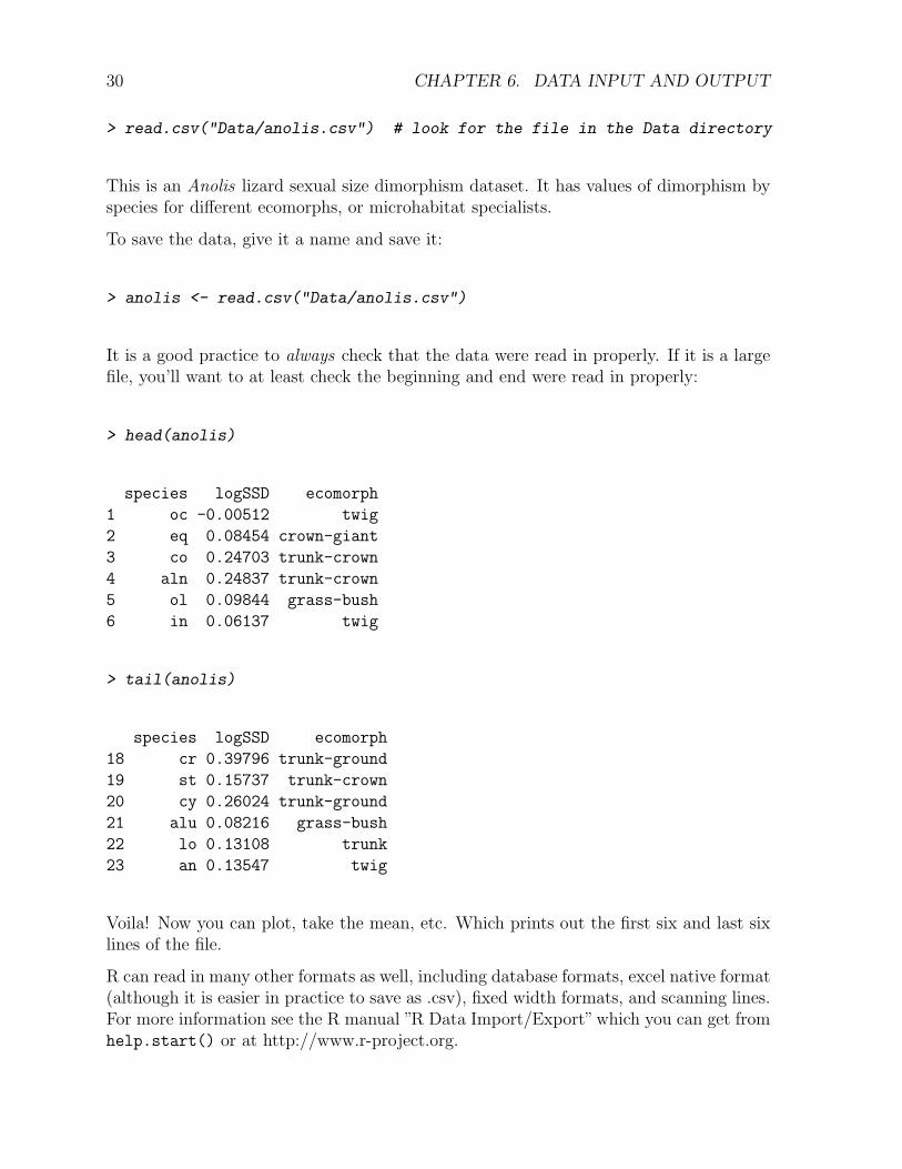
> read.csv("Data/anolis.csv") # look for the file in the Data directory
This is an Anolis lizard sexual size dimorphism dataset. It has values of dimorphism byspecies for different ecomorphs, or microhabitat specialists.
To save the data, give it a name and save it:
> anolis <- read.csv("Data/anolis.csv")
It is a good practice to always check that the data were read in properly. If it is a largefile, you’ll want to at least check the beginning and end were read in properly:
> head(anolis)
species logSSD ecomorph
1 oc -0.00512 twig
2 eq 0.08454 crown-giant
3 co 0.24703 trunk-crown
4 aln 0.24837 trunk-crown
5 ol 0.09844 grass-bush
6 in 0.06137 twig
> tail(anolis)
species logSSD ecomorph
18 cr 0.39796 trunk-ground
19 st 0.15737 trunk-crown
20 cy 0.26024 trunk-ground
21 alu 0.08216 grass-bush
22 lo 0.13108 trunk
23 an 0.13547 twig
Voila! Now you can plot, take the mean, etc. Which prints out the first six and last sixlines of the file.
R can read in many other formats as well, including database formats, excel native format(although it is easier in practice to save as .csv), fixed width formats, and scanning lines.For more information see the R manual ”R Data Import/Export” which you can get fromhelp.start() or at http://www.r-project.org.
6.2. SUMMARY STATISTICS ON YOUR DATA 31
6.2 Summary statistics on your data
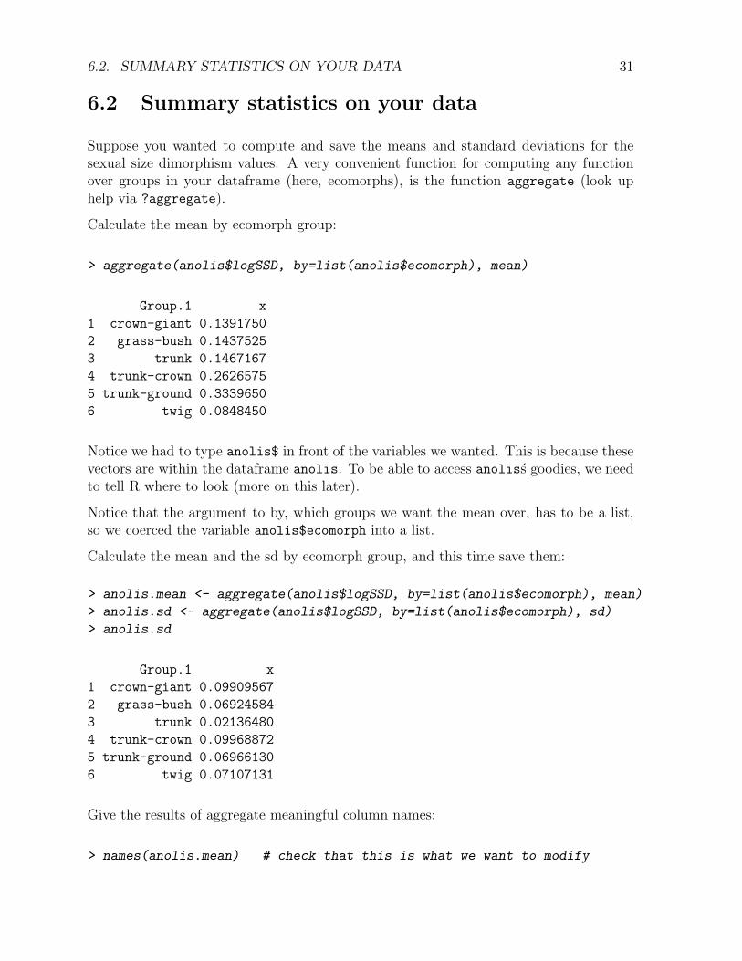
Suppose you wanted to compute and save the means and standard deviations for thesexual size dimorphism values. A very convenient function for computing any functionover groups in your dataframe (here, ecomorphs), is the function aggregate (look uphelp via ?aggregate).
Calculate the mean by ecomorph group:
> aggregate(anolis$logSSD, by=list(anolis$ecomorph), mean)
Group.1 x
1 crown-giant 0.1391750
2 grass-bush 0.1437525
3 trunk 0.1467167
4 trunk-crown 0.2626575
5 trunk-ground 0.3339650
6 twig 0.0848450
Notice we had to type anolis$ in front of the variables we wanted. This is because thesevectors are within the dataframe anolis. To be able to access anoliss goodies, we needto tell R where to look (more on this later).
Notice that the argument to by, which groups we want the mean over, has to be a list,so we coerced the variable anolis$ecomorph into a list.
Calculate the mean and the sd by ecomorph group, and this time save them:
> anolis.mean <- aggregate(anolis$logSSD, by=list(anolis$ecomorph), mean)
> anolis.sd <- aggregate(anolis$logSSD, by=list(anolis$ecomorph), sd)
> anolis.sd
Group.1 x
1 crown-giant 0.09909567
2 grass-bush 0.06924584
3 trunk 0.02136480
4 trunk-crown 0.09968872
5 trunk-ground 0.06966130
6 twig 0.07107131
Give the results of aggregate meaningful column names:
> names(anolis.mean) # check that this is what we want to modify
32 CHAPTER 6. DATA INPUT AND OUTPUT
[1] "Group.1" "x"
> names(anolis.mean) <- c("ecomorph", "mean")
> names(anolis.sd) <- c("ecomorph", "sd")
While we’re at it, let’s get the sample size so that we can calculate the standard error,which is the standard deviation divided by the square root of the sample size.
> anolis.N <- aggregate(anolis$logSSD, by=list(anolis$ecomorph), length)
> names(anolis.N) <- c("ecomorph", "N")
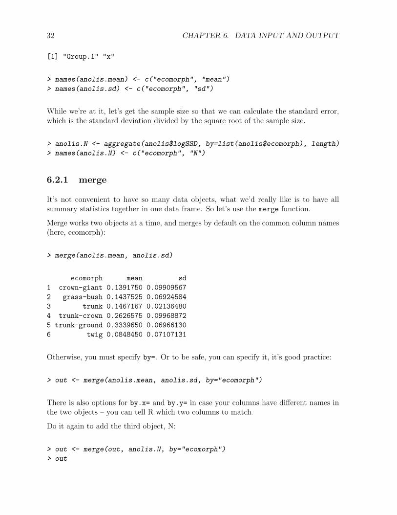
6.2.1 merge
It’s not convenient to have so many data objects, what we’d really like is to have allsummary statistics together in one data frame. So let’s use the merge function.
Merge works two objects at a time, and merges by default on the common column names(here, ecomorph):
> merge(anolis.mean, anolis.sd)
ecomorph mean sd
1 crown-giant 0.1391750 0.09909567
2 grass-bush 0.1437525 0.06924584
3 trunk 0.1467167 0.02136480
4 trunk-crown 0.2626575 0.09968872
5 trunk-ground 0.3339650 0.06966130
6 twig 0.0848450 0.07107131
Otherwise, you must specify by=. Or to be safe, you can specify it, it’s good practice:
> out <- merge(anolis.mean, anolis.sd, by="ecomorph")
There is also options for by.x= and by.y= in case your columns have different names inthe two objects – you can tell R which two columns to match.
Do it again to add the third object, N:
> out <- merge(out, anolis.N, by="ecomorph")
> out
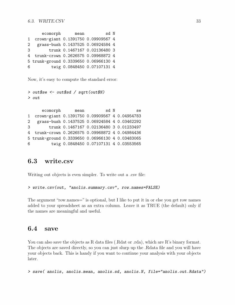
6.3. WRITE.CSV 33
ecomorph mean sd N
1 crown-giant 0.1391750 0.09909567 4
2 grass-bush 0.1437525 0.06924584 4
3 trunk 0.1467167 0.02136480 3
4 trunk-crown 0.2626575 0.09968872 4
5 trunk-ground 0.3339650 0.06966130 4
6 twig 0.0848450 0.07107131 4
Now, it’s easy to compute the standard error:
> out$se <- out$sd / sqrt(out$N)
> out
ecomorph mean sd N se
1 crown-giant 0.1391750 0.09909567 4 0.04954783
2 grass-bush 0.1437525 0.06924584 4 0.03462292
3 trunk 0.1467167 0.02136480 3 0.01233497
4 trunk-crown 0.2626575 0.09968872 4 0.04984436
5 trunk-ground 0.3339650 0.06966130 4 0.03483065
6 twig 0.0848450 0.07107131 4 0.03553565
6.3 write.csv
Writing out objects is even simpler. To write out a .csv file:
> write.csv(out, "anolis.summary.csv", row.names=FALSE)
The argument “row.names=” is optional, but I like to put it in or else you get row namesadded to your spreadsheet as an extra column. Leave it as TRUE (the default) only ifthe names are meaningful and useful.
6.4 save
You can also save the objects as R data files (.Rdat or .rda), which are R’s binary format.The objects are saved directly, so you can just slurp up the .Rdata file and you will haveyour objects back. This is handy if you want to continue your analysis with your objectslater.
> save( anolis, anolis.mean, anolis.sd, anolis.N, file="anolis.out.Rdata")
34 CHAPTER 6. DATA INPUT AND OUTPUT
The command to load these back in is:
> load("anolis.out.Rdata")
Which will restore your objects.
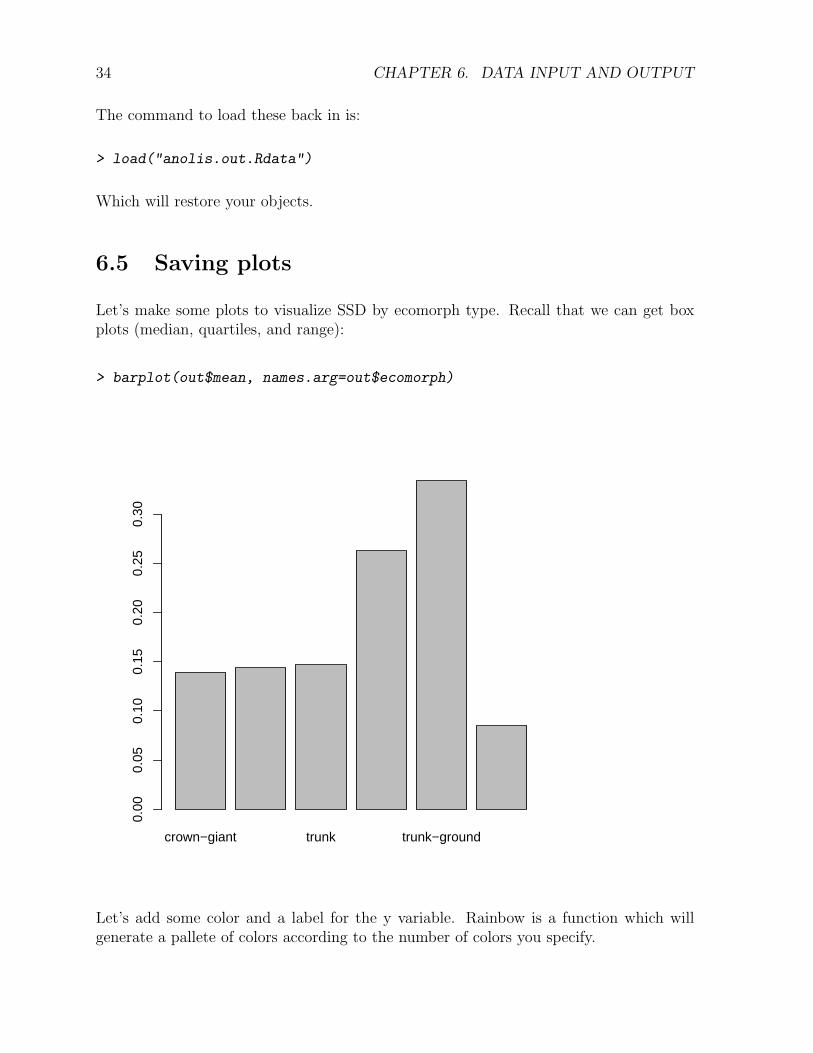
6.5 Saving plots
Let’s make some plots to visualize SSD by ecomorph type. Recall that we can get boxplots (median, quartiles, and range):
> barplot(out$mean, names.arg=out$ecomorph)
crown−giant trunk trunk−ground
0.00
0.05
0.10
0.15
0.20
0.25
0.30
Let’s add some color and a label for the y variable. Rainbow is a function which willgenerate a pallete of colors according to the number of colors you specify.
6.5. SAVING PLOTS 35
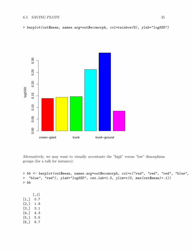
> barplot(out$mean, names.arg=out$ecomorph, col=rainbow(6), ylab="logSSD")
crown−giant trunk trunk−ground
logS
SD
0.00
0.05
0.10
0.15
0.20
0.25
0.30
Alternatively, we may want to visually accentuate the ”high” versus ”low” dimorphismgroups (for a talk for instance):
> bb <- barplot(out$mean, names.arg=out$ecomorph, col=c("red", "red", "red", "blue",
+ "blue", "red"), ylab="logSSD", cex.lab=1.5, ylim=c(0, max(out$mean)+.1))
> bb
[,1]
[1,] 0.7
[2,] 1.9
[3,] 3.1
[4,] 4.3
[5,] 5.5
[6,] 6.7
36 CHAPTER 6. DATA INPUT AND OUTPUT
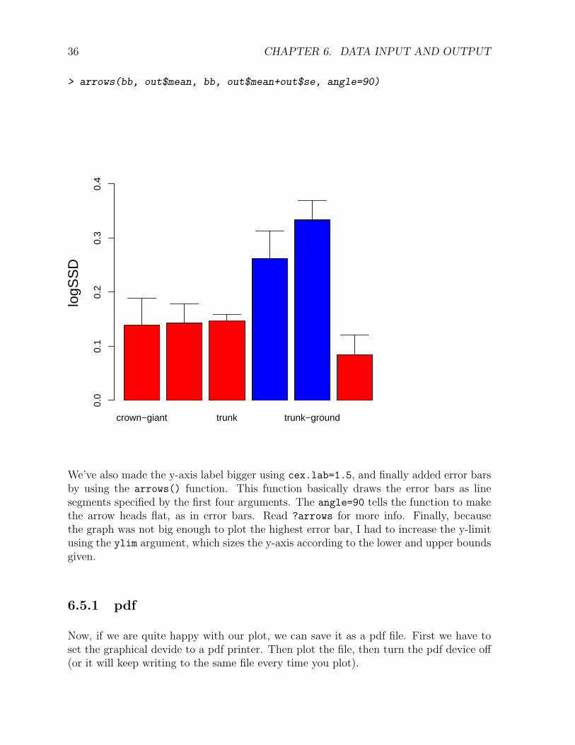
> arrows(bb, out$mean, bb, out$mean+out$se, angle=90)
crown−giant trunk trunk−ground
logS
SD
0.0
0.1
0.2
0.3
0.4
We’ve also made the y-axis label bigger using cex.lab=1.5, and finally added error barsby using the arrows() function. This function basically draws the error bars as linesegments specified by the first four arguments. The angle=90 tells the function to makethe arrow heads flat, as in error bars. Read ?arrows for more info. Finally, becausethe graph was not big enough to plot the highest error bar, I had to increase the y-limitusing the ylim argument, which sizes the y-axis according to the lower and upper boundsgiven.
6.5.1 pdf
Now, if we are quite happy with our plot, we can save it as a pdf file. First we have toset the graphical devide to a pdf printer. Then plot the file, then turn the pdf device off(or it will keep writing to the same file every time you plot).

6.6. MESSIER INPUT FILES 37
> pdf(file="anolisMeanSSD.pdf") # turns on the pdf device for plotting
> barplot(out$mean, names.arg=out$ecomorph, col=c("red", "red", "red", "blue",
+ "blue", "red"), ylab="logSSD", cex.lab=1.5)
> dev.off() # turns off pdf device for output
quartz
2
6.6 Messier input files
The first example of a csv file was very easy to bring in to R. If it was hand-entered, youmay have several issues including:
• extra delimiters in some rows (extra commas, etc.) so that some rows have extracolumns
• extra header lines
• lots of missing values
• mixed character and numeric input
Any of these issues will cause problems because what you are reading in is a data frame.R expects columns to be of the same type, and the object is square, and etc.
Extra header lines are really easy to fix using the skip= option. However, the otherissues will have to be fixed by editing your .csv file, or by writing code that reads in thelines one by one, makes the appropriate changes, and then writing out a “clean” .csv file.Which way to go should be determined by how much work it will be to hand-edit vs.program, which will depend a lot on how many problems the file contains, and whetherthey are unique or not. (Probably 80% or more of your R programming efforts are aimedat getting your input data into shape for analysis – which is why we cover these in thenext section).
6.6.1 Input files generated by data loggers
An easier case to handle: files that are generated by computer. Take, for example, the fileformat generated from our hand-held Ocean Optics specroradiometer. It is very regularin structure, and we have tons of data files, so it is well worth the programming effort tocode a script for automatic file input.
First, you can open the file below in a text editor. If you’d rather open it in R, you canuse:
38 CHAPTER 6. DATA INPUT AND OUTPUT
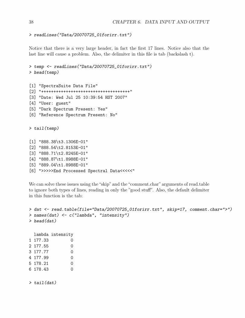
> readLines("Data/20070725_01forirr.txt")
Notice that there is a very large header, in fact the first 17 lines. Notice also that thelast line will cause a problem. Also, the delimiter in this file is tab (backslash t).
> temp <- readLines("Data/20070725_01forirr.txt")
> head(temp)
[1] "SpectraSuite Data File"
[2] "++++++++++++++++++++++++++++++++++++"
[3] "Date: Wed Jul 25 10:39:54 HST 2007"
[4] "User: guest"
[5] "Dark Spectrum Present: Yes"
[6] "Reference Spectrum Present: No"
> tail(temp)
[1] "888.38\t3.1306E-01"
[2] "888.54\t2.8153E-01"
[3] "888.71\t2.8245E-01"
[4] "888.87\t1.8988E-01"
[5] "889.04\t1.8988E-01"
[6] ">>>>>End Processed Spectral Data<<<<<"
We can solve these issues using the“skip”and the“comment.char”arguments of read.tableto ignore both types of lines, reading in only the ”good stuff”. Also, the default delimiterin this function is the tab:
> dat <- read.table(file="Data/20070725_01forirr.txt", skip=17, comment.char=">")
> names(dat) <- c("lambda", "intensity")
> head(dat)
lambda intensity
1 177.33 0
2 177.55 0
3 177.77 0
4 177.99 0
5 178.21 0
6 178.43 0
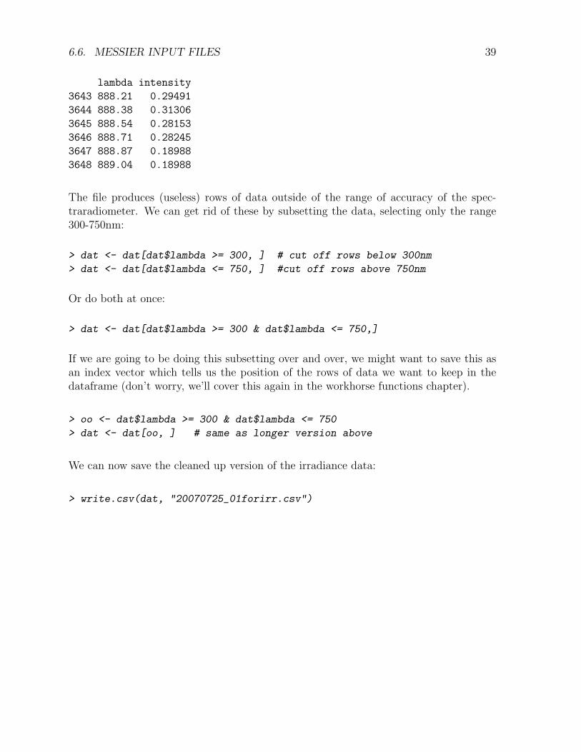
> tail(dat)
6.6. MESSIER INPUT FILES 39
lambda intensity
3643 888.21 0.29491
3644 888.38 0.31306
3645 888.54 0.28153
3646 888.71 0.28245
3647 888.87 0.18988
3648 889.04 0.18988
The file produces (useless) rows of data outside of the range of accuracy of the spec-traradiometer. We can get rid of these by subsetting the data, selecting only the range300-750nm:
> dat <- dat[dat$lambda >= 300, ] # cut off rows below 300nm
> dat <- dat[dat$lambda <= 750, ] #cut off rows above 750nm
Or do both at once:
> dat <- dat[dat$lambda >= 300 & dat$lambda <= 750,]
If we are going to be doing this subsetting over and over, we might want to save this asan index vector which tells us the position of the rows of data we want to keep in thedataframe (don’t worry, we’ll cover this again in the workhorse functions chapter).
> oo <- dat$lambda >= 300 & dat$lambda <= 750
> dat <- dat[oo, ] # same as longer version above
We can now save the cleaned up version of the irradiance data:
> write.csv(dat, "20070725_01forirr.csv")

40 CHAPTER 6. DATA INPUT AND OUTPUT
Chapter 7
The Workhorse Functions of DataManipulation
Chapter Topics/Skills:
Indexing/Subsetting accessing particular elements of your dataframe
String Matching using grep, sub
Sorting ordering data
Matching using logical comparisons to index
Merging matching two data frames or matrices by a common column and merging intoa new object
Reshaping R Objects changing the shape of matrices and dataframes, long-thin toshort-fat formats
Attributes, Classes the characteristics of data objects and how to manipulate them
As a biologist, these data manipulation topics may seem dry, but they are really pow-erful and will allow you do to much more sophisticated analyses, and to do them withconfidence. So it is well worth taking some time to learn how to use them well.
7.1 Indexing and subsetting
R has powerful database functionality. Subsetting (picking particular observations outof an R object) is something that you will have to do all the time.
41
42 CHAPTER 7. THE WORKHORSE FUNCTIONS OF DATA MANIPULATION
Let’s work with a dataframe that is provided with the phylobase package called geospiza_raw.It contains five morphological measurements for 13 species. First, let’s clear the workspace(or clear and start a new R session):
If you have the package phylobase installed, get the built-in dataset this way:
> rm(list=ls())
> require(phylobase)
> data(geospiza_raw) # load the dataset into the workspace
> ls() # list the objects in the workspace
[1] "geospiza_raw"
The object was named geospiza_raw. Let’s find out some basic information about thisobject:
> class(geospiza_raw)
[1] "list"
> attributes(geospiza_raw)
$names
[1] "tree" "data"
It is a list with two elements. Here we want the data
> geo <- geospiza_raw$data
> dim(geo)
[1] 13 5
If you don’t have phylobase installed, then please read in this .csv input file and proceed.
> geo <- read.csv("Data/geospiza_raw.csv")
> dim(geo)
It is a dataframe with 13 rows and 5 columns. If we want to know all the attributes ofgeo:

7.1. INDEXING AND SUBSETTING 43
> attributes(geo)
$names
[1] "wingL" "tarsusL" "culmenL" "beakD" "gonysW"
$row.names
[1] "fuliginosa" "fortis" "magnirostris" "conirostris" "scandens"
[6] "difficilis" "pallida" "parvulus" "psittacula" "pauper"
[11] "Platyspiza" "fusca" "Pinaroloxias"
$class
[1] "data.frame"
We see that it has a ”names” attribute, which refers to column names in a dataframe.Typically, the columns of a dataframe are the variables in the dataset. It also has”rownames” which contains the species names (so it does not have a separate column forspecies names).
In general, accessing elements of vectors, matrices, or dataframes is achieved throughindexing by:
inclusion a vector of positive integers indicating which elements of the vector to include
exclusion a vector of negative integers
logical values a vector of TRUE / FALSE values indicating which elements to include/ exclude
by name a character vector of names of columns (only) or columns and rows
blank index take the entire column, row, or object
Dataframes have two dimensions which we can use to index with: dataframe[row, col-umn].
> geo # the entire object, same as geo[] or geo[,]
> geo[c(1, 3), ] # select the first and third rows, all columns
> geo[, 3:5] # all rows, third through fifth columns
> geo[1, 5] # first row, fifth column (a single number)
> geo[1:2, c(3, 1)] # first and second row, third and first column (2x2 matrix)
> geo[-c(1:3, 10:13), ] # everything but the first three and last three rows
> geo[ 1:3, 5:1] # first three species, but variables in reverse order
Indexing a data frame by a single vector (meaning, no comma separating) selects anentire column. This can be done by name or by number:
44 CHAPTER 7. THE WORKHORSE FUNCTIONS OF DATA MANIPULATION
> geo[3] # third column
> geo["culmenL"] # same
> geo[c(3,5)] # third and fifth column
> geo[c("culmenL", "gonysW")] # same
We can also use the names (or rownames) attribute if we are lazy. Suppose we wantedall the species which began with ”pa”. we could find which position they hold in thedataframe by looking at the rownames, saving them to a vector, and then indexing bythem:
> sp <- rownames(geo)
> sp # a vector of the species names
[1] "fuliginosa" "fortis" "magnirostris" "conirostris" "scandens"
[6] "difficilis" "pallida" "parvulus" "psittacula" "pauper"
[11] "Platyspiza" "fusca" "Pinaroloxias"
> sp[c(7,8,10)] # the ones we want are #7,8, and 10
[1] "pallida" "parvulus" "pauper"
> geo[ sp[c(7,8,10)], ] # rows 7,8 and 10, same as geo[c(7, 8, 10)]
wingL tarsusL culmenL beakD gonysW
pallida 4.265425 3.08945 2.43025 2.01635 1.949125
parvulus 4.131600 2.97306 1.97442 1.87354 1.813340
pauper 4.232500 3.03590 2.18700 2.07340 1.962100
An equivalent way to index is by using the subset function. Some people prefer itbecause you have explicit parameters for what to select and which variables to include.See help page ?subset.
7.2 String Matching
A more useful feature is string matching. R has grep facilities, which can do partialmatching of character strings. For example, we could directly search for species (theobject or ”x”) names which contain ”p” (the pattern):
> sp <- rownames(geo)
> grep(pattern = "p", x = sp) # returns indices

7.3. ORDERING DATA 45
[1] 7 8 9 10 11
> grep("p", sp, value=T) # returns the species names which match
[1] "pallida" "parvulus" "psittacula" "pauper" "Platyspiza"
> grep("p", sp, ignore.case=T, value=T) # case-sensitive by default
[1] "pallida" "parvulus" "psittacula" "pauper" "Platyspiza"
[6] "Pinaroloxias"
> grep("^P", sp, value=T) # only those which start with (^) capital P
[1] "Platyspiza" "Pinaroloxias"
It is possible to use perl-type regular expressions, and the sub function is also available.Sub is related to grep, but substitutes a replacement value to the matched pattern. Noticethat there are two species which have upper case letters. We can fix this with:
> sp <- rownames(geo)
> sub(pattern = "^P", replacement = "p", sp)
[1] "fuliginosa" "fortis" "magnirostris" "conirostris" "scandens"
[6] "difficilis" "pallida" "parvulus" "psittacula" "pauper"
[11] "platyspiza" "fusca" "pinaroloxias"
> rownames(geo) <- sub(pattern = "^P", replacement = "p", sp) # to save changes
7.3 Ordering Data
Suppose we now want geo in alphabetical order. We can use the sort function to sortthe rownames vector, then use it to index the dataframe:
> sort(rownames(geo))
> geo[ sort(rownames(geo)), ]
A better option for dataframes, though, is order:
46 CHAPTER 7. THE WORKHORSE FUNCTIONS OF DATA MANIPULATION
> order(rownames(geo)) # the order that the species should take to be
[1] 4 6 2 1 12 3 7 8 10 13 11 9 5
> # sorted from a-z
> rbind(rownames(geo), order(rownames(geo))) # to illustrate
[,1] [,2] [,3] [,4] [,5] [,6]
[1,] "fuliginosa" "fortis" "magnirostris" "conirostris" "scandens" "difficilis"
[2,] "4" "6" "2" "1" "12" "3"
[,7] [,8] [,9] [,10] [,11] [,12]
[1,] "pallida" "parvulus" "psittacula" "pauper" "platyspiza" "fusca"
[2,] "7" "8" "10" "13" "11" "9"
[,13]
[1,] "pinaroloxias"
[2,] "5"
> oo <- order(rownames(geo))
> geo[oo,] # sorted in alpha order
wingL tarsusL culmenL beakD gonysW
conirostris 4.349867 2.984200 2.654400 2.513800 2.360167
difficilis 4.224067 2.898917 2.277183 2.011100 1.929983
fortis 4.244008 2.894717 2.407025 2.362658 2.221867
fuliginosa 4.132957 2.806514 2.094971 1.941157 1.845379
fusca 3.975393 2.936536 2.051843 1.191264 1.401186
magnirostris 4.404200 3.038950 2.724667 2.823767 2.675983
pallida 4.265425 3.089450 2.430250 2.016350 1.949125
parvulus 4.131600 2.973060 1.974420 1.873540 1.813340
pauper 4.232500 3.035900 2.187000 2.073400 1.962100
pinaroloxias 4.188600 2.980200 2.311100 1.547500 1.630100
platyspiza 4.419686 3.270543 2.331471 2.347471 2.282443
psittacula 4.235020 3.049120 2.259640 2.230040 2.073940
scandens 4.261222 2.929033 2.621789 2.144700 2.036944
Order can sort on multiple arguments, which means that you can use other columns tobreak ties. Let’s trim the species names to the first letter using the substring function,then sort using the first letter of the species name and breaking ties by tarsusL:
> sp <- substring(rownames(geo), first=1, last=1)
> oo <- order(sp , geo$tarsusL) # order by first letter species, then tarsusL
> geot <- geo[oo,]["tarsusL"] # ordered geo dataframe, take only the wingL column
> geo <- geo[oo,]
7.4. MATCHING 47
Note: using geo["tarsusL"] as a second index for order doesn’t work, because it is a onecolumn dataframe, as opposed to geo$tarsus which is a vector. It must match sp, whichis a vector. Check the dim and length of each. vectors have length only, dataframeshave dimension 2.
7.4 Matching
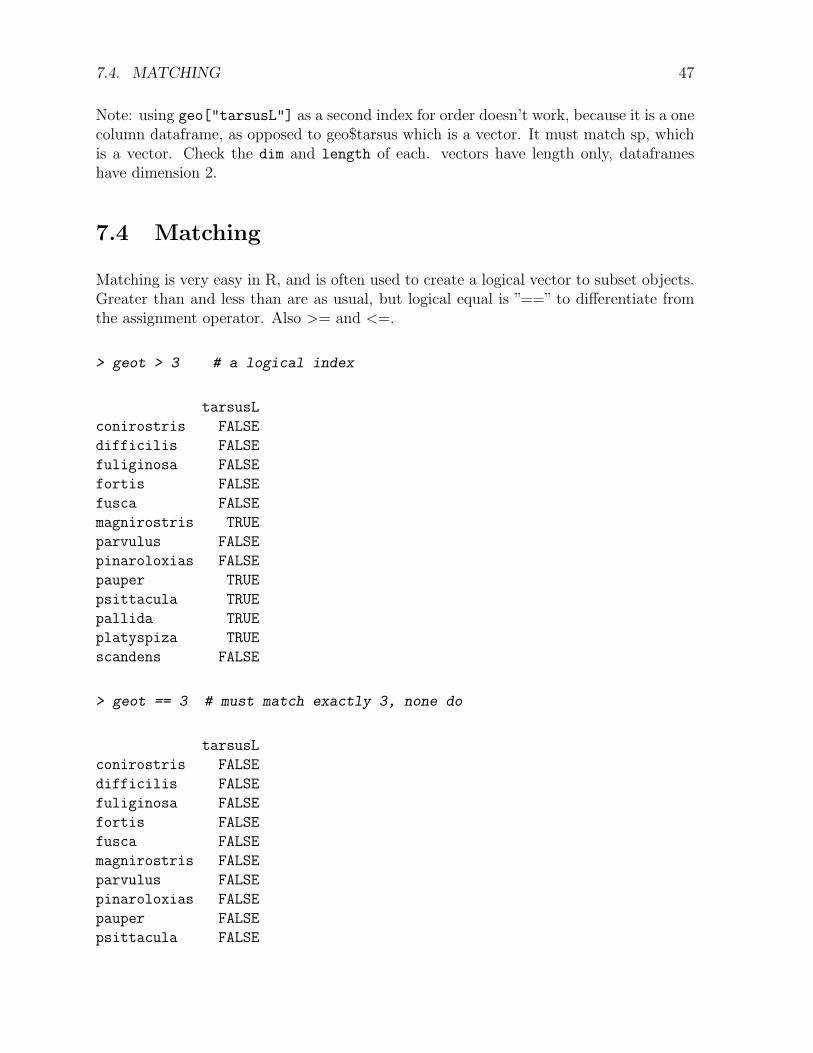
Matching is very easy in R, and is often used to create a logical vector to subset objects.Greater than and less than are as usual, but logical equal is ”==” to differentiate fromthe assignment operator. Also >= and <=.
> geot > 3 # a logical index
tarsusL
conirostris FALSE
difficilis FALSE
fuliginosa FALSE
fortis FALSE
fusca FALSE
magnirostris TRUE
parvulus FALSE
pinaroloxias FALSE
pauper TRUE
psittacula TRUE
pallida TRUE
platyspiza TRUE
scandens FALSE
> geot == 3 # must match exactly 3, none do
tarsusL
conirostris FALSE
difficilis FALSE
fuliginosa FALSE
fortis FALSE
fusca FALSE
magnirostris FALSE
parvulus FALSE
pinaroloxias FALSE
pauper FALSE
psittacula FALSE
48 CHAPTER 7. THE WORKHORSE FUNCTIONS OF DATA MANIPULATION
pallida FALSE
platyspiza FALSE
scandens FALSE
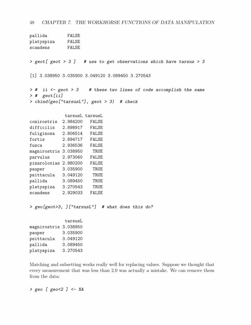
> geot[ geot > 3 ] # use to get observations which have tarsus > 3
[1] 3.038950 3.035900 3.049120 3.089450 3.270543
> # ii <- geot > 3 # these two lines of code accomplish the same
> # geot[ii]
> cbind(geo["tarsusL"], geot > 3) # check
tarsusL tarsusL
conirostris 2.984200 FALSE
difficilis 2.898917 FALSE
fuliginosa 2.806514 FALSE
fortis 2.894717 FALSE
fusca 2.936536 FALSE
magnirostris 3.038950 TRUE
parvulus 2.973060 FALSE
pinaroloxias 2.980200 FALSE
pauper 3.035900 TRUE
psittacula 3.049120 TRUE
pallida 3.089450 TRUE
platyspiza 3.270543 TRUE
scandens 2.929033 FALSE
> geo[geot>3, ]["tarsusL"] # what does this do?
tarsusL
magnirostris 3.038950
pauper 3.035900
psittacula 3.049120
pallida 3.089450
platyspiza 3.270543
Matching and subsetting works really well for replacing values. Suppose we thought thatevery measurement that was less than 2.0 was actually a mistake. We can remove themfrom the data:
> geo [ geo<2 ] <- NA
7.4. MATCHING 49
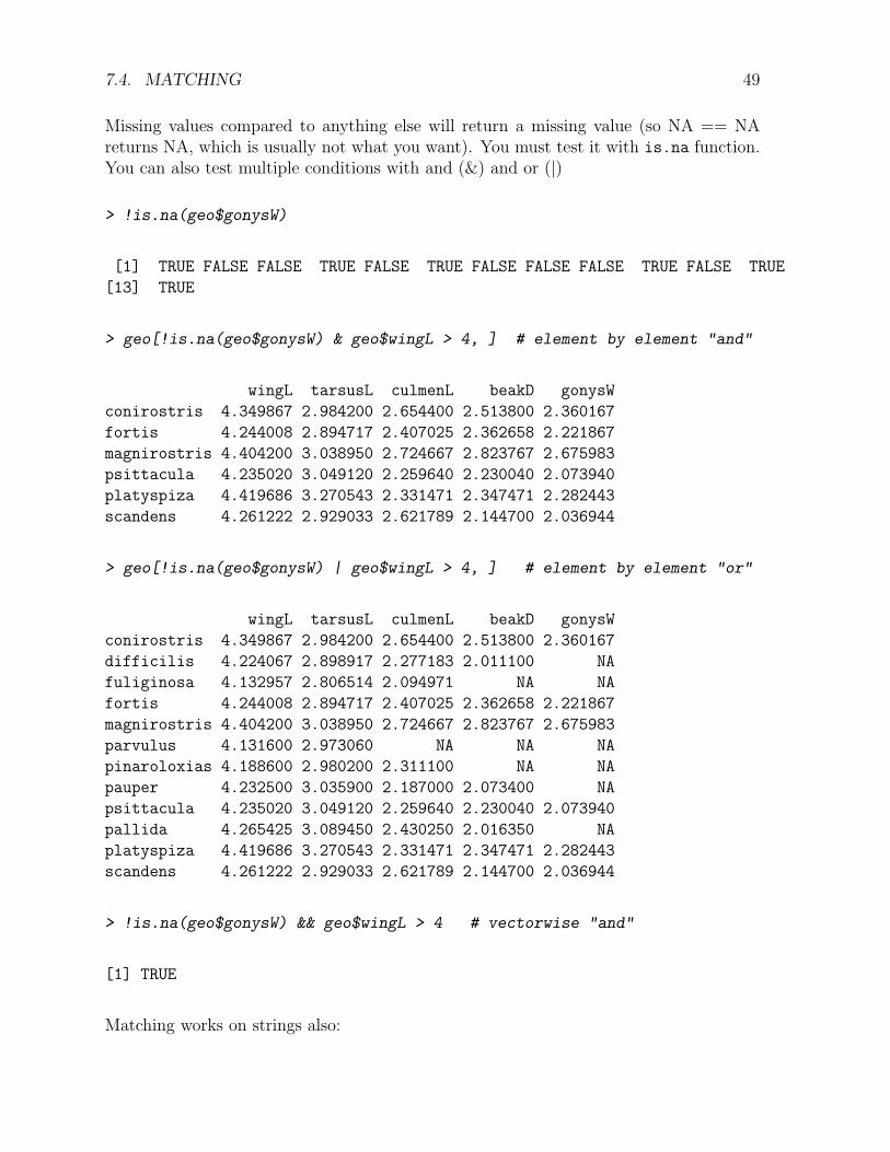
Missing values compared to anything else will return a missing value (so NA == NAreturns NA, which is usually not what you want). You must test it with is.na function.You can also test multiple conditions with and (&) and or (|)
> !is.na(geo$gonysW)
[1] TRUE FALSE FALSE TRUE FALSE TRUE FALSE FALSE FALSE TRUE FALSE TRUE
[13] TRUE
> geo[!is.na(geo$gonysW) & geo$wingL > 4, ] # element by element "and"
wingL tarsusL culmenL beakD gonysW
conirostris 4.349867 2.984200 2.654400 2.513800 2.360167
fortis 4.244008 2.894717 2.407025 2.362658 2.221867
magnirostris 4.404200 3.038950 2.724667 2.823767 2.675983
psittacula 4.235020 3.049120 2.259640 2.230040 2.073940
platyspiza 4.419686 3.270543 2.331471 2.347471 2.282443
scandens 4.261222 2.929033 2.621789 2.144700 2.036944
> geo[!is.na(geo$gonysW) | geo$wingL > 4, ] # element by element "or"
wingL tarsusL culmenL beakD gonysW
conirostris 4.349867 2.984200 2.654400 2.513800 2.360167
difficilis 4.224067 2.898917 2.277183 2.011100 NA
fuliginosa 4.132957 2.806514 2.094971 NA NA
fortis 4.244008 2.894717 2.407025 2.362658 2.221867
magnirostris 4.404200 3.038950 2.724667 2.823767 2.675983
parvulus 4.131600 2.973060 NA NA NA
pinaroloxias 4.188600 2.980200 2.311100 NA NA
pauper 4.232500 3.035900 2.187000 2.073400 NA
psittacula 4.235020 3.049120 2.259640 2.230040 2.073940
pallida 4.265425 3.089450 2.430250 2.016350 NA
platyspiza 4.419686 3.270543 2.331471 2.347471 2.282443
scandens 4.261222 2.929033 2.621789 2.144700 2.036944
> !is.na(geo$gonysW) && geo$wingL > 4 # vectorwise "and"
[1] TRUE
Matching works on strings also:
50 CHAPTER 7. THE WORKHORSE FUNCTIONS OF DATA MANIPULATION
> geo[rownames(geo) == "pauper",] # same as geo["pauper", ]
> geo[rownames(geo) < "pauper",]
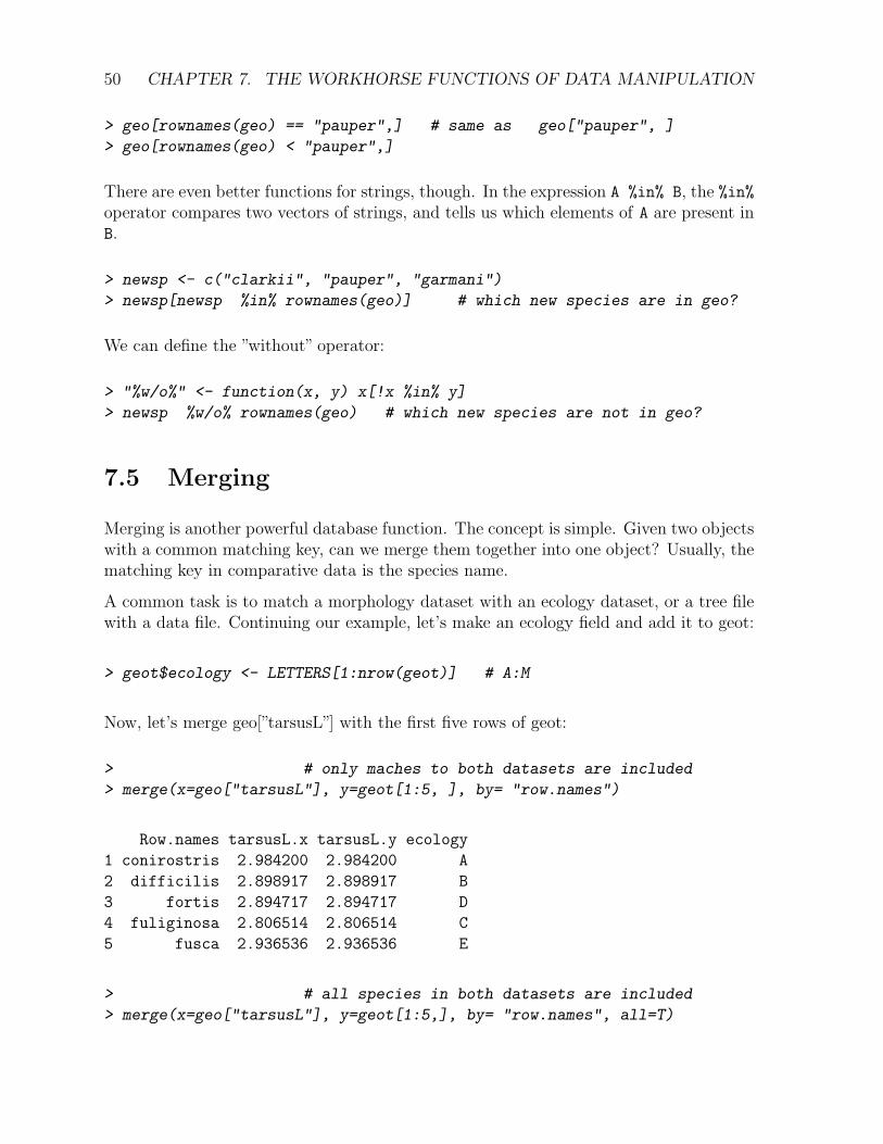
There are even better functions for strings, though. In the expression A %in% B, the %in%operator compares two vectors of strings, and tells us which elements of A are present inB.
> newsp <- c("clarkii", "pauper", "garmani")
> newsp[newsp %in% rownames(geo)] # which new species are in geo?
We can define the ”without” operator:
> "%w/o%" <- function(x, y) x[!x %in% y]
> newsp %w/o% rownames(geo) # which new species are not in geo?
7.5 Merging
Merging is another powerful database function. The concept is simple. Given two objectswith a common matching key, can we merge them together into one object? Usually, thematching key in comparative data is the species name.
A common task is to match a morphology dataset with an ecology dataset, or a tree filewith a data file. Continuing our example, let’s make an ecology field and add it to geot:
> geot$ecology <- LETTERS[1:nrow(geot)] # A:M
Now, let’s merge geo[”tarsusL”] with the first five rows of geot:
> # only maches to both datasets are included
> merge(x=geo["tarsusL"], y=geot[1:5, ], by= "row.names")
Row.names tarsusL.x tarsusL.y ecology
1 conirostris 2.984200 2.984200 A
2 difficilis 2.898917 2.898917 B
3 fortis 2.894717 2.894717 D
4 fuliginosa 2.806514 2.806514 C
5 fusca 2.936536 2.936536 E
> # all species in both datasets are included
> merge(x=geo["tarsusL"], y=geot[1:5,], by= "row.names", all=T)
7.6. RESHAPING R OBJECTS 51
Row.names tarsusL.x tarsusL.y ecology
1 conirostris 2.984200 2.984200 A
2 difficilis 2.898917 2.898917 B
3 fortis 2.894717 2.894717 D
4 fuliginosa 2.806514 2.806514 C
5 fusca 2.936536 2.936536 E
6 magnirostris 3.038950 NA <NA>
7 pallida 3.089450 NA <NA>
8 parvulus 2.973060 NA <NA>
9 pauper 3.035900 NA <NA>
10 pinaroloxias 2.980200 NA <NA>
11 platyspiza 3.270543 NA <NA>
12 psittacula 3.049120 NA <NA>
13 scandens 2.929033 NA <NA>
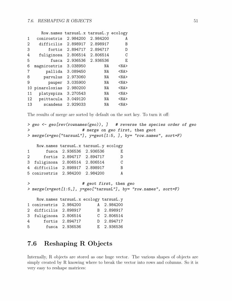
The results of merge are sorted by default on the sort key. To turn it off:
> geo <- geo[rev(rownames(geo)), ] # reverse the species order of geo
> # merge on geo first, then geot
> merge(x=geo["tarsusL"], y=geot[1:5, ], by= "row.names", sort=F)
Row.names tarsusL.x tarsusL.y ecology
1 fusca 2.936536 2.936536 E
2 fortis 2.894717 2.894717 D
3 fuliginosa 2.806514 2.806514 C
4 difficilis 2.898917 2.898917 B
5 conirostris 2.984200 2.984200 A
> # geot first, then geo
> merge(x=geot[1:5,], y=geo["tarsusL"], by= "row.names", sort=F)
Row.names tarsusL.x ecology tarsusL.y
1 conirostris 2.984200 A 2.984200
2 difficilis 2.898917 B 2.898917
3 fuliginosa 2.806514 C 2.806514
4 fortis 2.894717 D 2.894717
5 fusca 2.936536 E 2.936536
7.6 Reshaping R Objects
Internally, R objects are stored as one huge vector. The various shapes of objects aresimply created by R knowing where to break the vector into rows and columns. So it isvery easy to reshape matrices:

52 CHAPTER 7. THE WORKHORSE FUNCTIONS OF DATA MANIPULATION
> vv <- 1:10 # a vector
> mm <- matrix( vv, nrow=2) # a matrix
> mm
[,1] [,2] [,3] [,4] [,5]
[1,] 1 3 5 7 9
[2,] 2 4 6 8 10
> dim(mm) <- NULL
> mm <- matrix( vv, nrow=2, byrow=T) # a matrix, but cells are now filled by row
> mm
[,1] [,2] [,3] [,4] [,5]
[1,] 1 2 3 4 5
[2,] 6 7 8 9 10
> dim(mm) <- NULL
> mm # vector is now n a different order because the collapse occurred by column
[1] 1 6 2 7 3 8 4 9 5 10
Other means of ”collapsing” dataframes are:
> unlist(geo) # produces a vector from the dataframe
> # the atomic type of a dataframe is a list
> unclass(geo) # removes the class attribute, turning the dataframe into a
> # series of vectors plus any names attributes, same as setting
> # class(geo) <- NULL
> c(geo) # similar to unclass but without the attributes
Practice
1. Recall from the chapter on Data Objects that we were simulating data in differenttreatment groups, and wanting to visualize the groups. Now that we know how toindex and subset, we can use the points function to add different colored pointsto the plot for different groups.
(a) Now let’s make some data which should differ. For the ”low” treatment, sim-ulate y and y1 as normally distributed data with mean = -2 and sd=.5, and”high” as mean=5, and sd=3. Remake the dataframe.
7.6. RESHAPING R OBJECTS 53
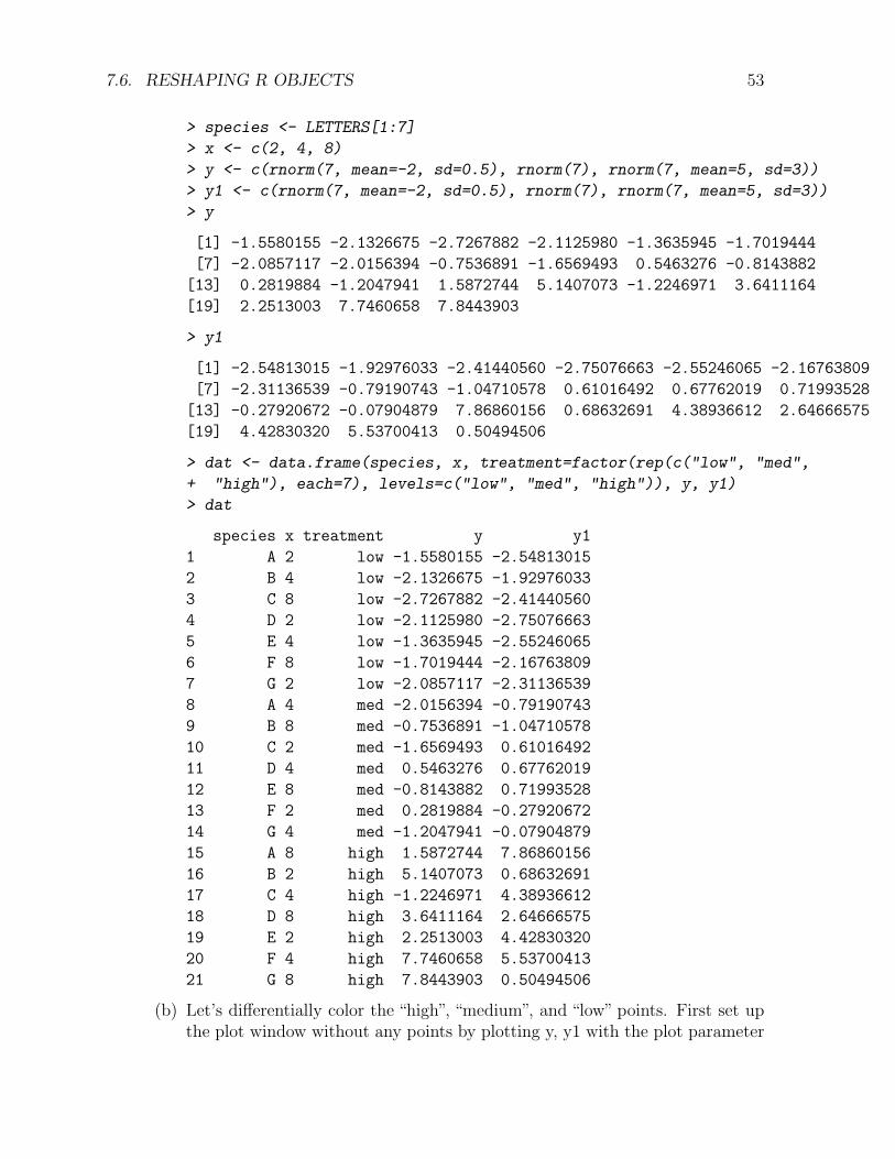
> species <- LETTERS[1:7]
> x <- c(2, 4, 8)
> y <- c(rnorm(7, mean=-2, sd=0.5), rnorm(7), rnorm(7, mean=5, sd=3))
> y1 <- c(rnorm(7, mean=-2, sd=0.5), rnorm(7), rnorm(7, mean=5, sd=3))
> y
[1] -1.5580155 -2.1326675 -2.7267882 -2.1125980 -1.3635945 -1.7019444
[7] -2.0857117 -2.0156394 -0.7536891 -1.6569493 0.5463276 -0.8143882
[13] 0.2819884 -1.2047941 1.5872744 5.1407073 -1.2246971 3.6411164
[19] 2.2513003 7.7460658 7.8443903
> y1
[1] -2.54813015 -1.92976033 -2.41440560 -2.75076663 -2.55246065 -2.16763809
[7] -2.31136539 -0.79190743 -1.04710578 0.61016492 0.67762019 0.71993528
[13] -0.27920672 -0.07904879 7.86860156 0.68632691 4.38936612 2.64666575
[19] 4.42830320 5.53700413 0.50494506
> dat <- data.frame(species, x, treatment=factor(rep(c("low", "med",
+ "high"), each=7), levels=c("low", "med", "high")), y, y1)
> dat
species x treatment y y1
1 A 2 low -1.5580155 -2.54813015
2 B 4 low -2.1326675 -1.92976033
3 C 8 low -2.7267882 -2.41440560
4 D 2 low -2.1125980 -2.75076663
5 E 4 low -1.3635945 -2.55246065
6 F 8 low -1.7019444 -2.16763809
7 G 2 low -2.0857117 -2.31136539
8 A 4 med -2.0156394 -0.79190743
9 B 8 med -0.7536891 -1.04710578
10 C 2 med -1.6569493 0.61016492
11 D 4 med 0.5463276 0.67762019
12 E 8 med -0.8143882 0.71993528
13 F 2 med 0.2819884 -0.27920672
14 G 4 med -1.2047941 -0.07904879
15 A 8 high 1.5872744 7.86860156
16 B 2 high 5.1407073 0.68632691
17 C 4 high -1.2246971 4.38936612
18 D 8 high 3.6411164 2.64666575
19 E 2 high 2.2513003 4.42830320
20 F 4 high 7.7460658 5.53700413
21 G 8 high 7.8443903 0.50494506
(b) Let’s differentially color the “high”, “medium”, and “low” points. First set upthe plot window without any points by plotting y, y1 with the plot parameter

54 CHAPTER 7. THE WORKHORSE FUNCTIONS OF DATA MANIPULATION
type="n". Then select only the ”high” points by subsetting. You’ll wantto make an index vector to choose only the points you want. Then use thepoints() function (which has the same form as the plot() function, butonly adds points to an existing plot. Choose three different colors for eachtreatment level and plot all the data. Is there any patterning in y, y1?
(c) Ooops! The data are actually supposed to be blocked by treatment (the firstseven rows correspond to low, the second 7 correspond to med, etc.) Can youremake the dataframe keeping the y and y1 in the same position, but fixingthe treatment?
(d) Make three plots: boxplot of treatment vs. y, treatment vs. y1, and three colorscatterplot of y vs. y1 (treatments should be indicated by different colors).
2. Matrix reshaping and indexing
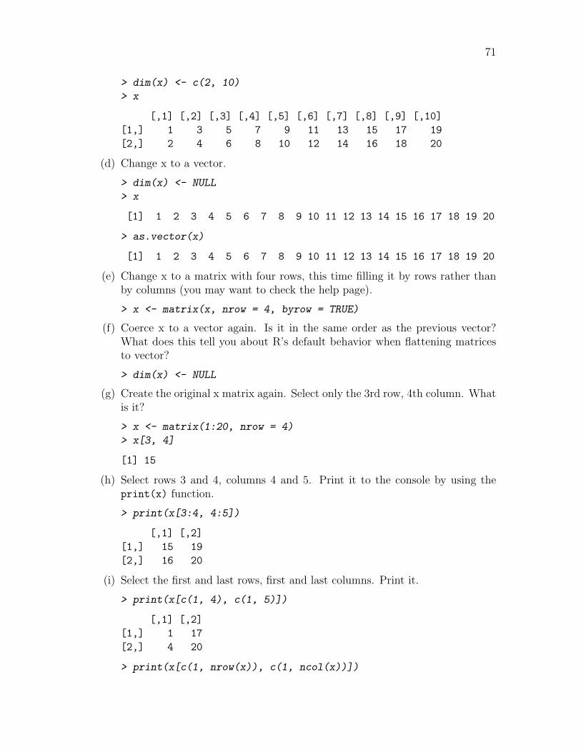
(a) Create a matrix with the values 1 through 20, filling four rows. Save it as “x”.item What are the attributes of x?
(b) Change it to a matrix with 2 rows and 10 columns by changing its attribute.item Change x to a vector.
(c) Change x to a matrix with four rows, this time filling it by rows rather thanby columns (you may want to check the help page).
(d) Coerce x to a vector again. Is it in the same order as the previous vector?What does this tell you about R’s default behavior when flattening matricesto vector?
(e) Create the original x matrix again. Select only the 3rd row, 4th column. Whatis it?
(f) Select rows 3 and 4, columns 4 and 5. Print it to the console by using theprint(x) function.
(g) Select the first and last rows, first and last columns. Print it.
3. Reading in Data and adding on
(a) Read in the external file bimac.csv in comma separated format. Save it as“bimac”.
(b) This is a phylogenetic tree and data for the OUCH package. Without goinginto details for now, this method allows biologists to specify selective regimeson branches of the phylogeny, by specifying categories which correspond toalternative “niches”. This is a body size evolution dataset, and “OU.LP” is ahypothesis with three size categories. We would like to make three additionalhypotheses. Add additional columns to this dataframe: OU.1 which has valuesof “global” for all rows, OU.3 which is the same as OU.LP, except those rowswith “NA” in the species names should get a value of “medium”, and OU.4which is again similar to OU.LP, except that those rows with “NA” in thespecies names get a value of “anc”.

Chapter 8
Answers to Exercises – CreatingData Objects
Practice
1. Create a dataset with simulated data using rnorm().
(a) Simulate 21 random data points drawn from a normal distribution (create anumeric vector), and save it in the variable “y”. Create a second set of 21points and save it as “y1”.
> y <- rnorm(21)
> y1 <- rnorm(21)
> y
[1] -1.7574988 -0.1199472 -2.1122496 -0.3110942 -0.2453429 0.5225224
[7] -1.1633751 -0.1948244 0.9785726 0.7678475 1.3574943 -0.3029250
[13] 0.6671354 0.0196097 -0.4265499 0.1839618 0.4749632 0.6700754
[19] 1.2702277 -0.5149302 0.8784322
> y1
[1] 1.11620178 -0.51097788 -1.27546731 -1.27632758 0.39144075 0.58795866
[7] 0.02636079 -2.40337715 -1.11326627 2.03374194 0.68305316 -0.73346041
[13] 2.54028332 1.09231928 0.89925111 -0.35779939 0.43452911 1.35573057
[19] 1.14789262 0.35294657 0.70047388
(b) Create a treatment vector with levels “low”, “med”, and “high”, save it as afactor.
> treatment <- factor( c("low", "med", "high") )
> treatment
[1] low med high
Levels: high low med
55

56 CHAPTER 8. ANSWERS TO EXERCISES – CREATING DATA OBJECTS
(c) Our treatment has numeric values also, so create a numeric vector with thevalues 2, 4, 8, save it as x.
> x <- c(2, 4, 8)
> x
[1] 2 4 8
(d) Create a species vector with seven names.
> species <- LETTERS[1:7]
> species
[1] "A" "B" "C" "D" "E" "F" "G"
(e) Create a matrix with y in the first column and x in the second column, saveit as dat.matrix.
> dat.matrix <- cbind( y, x )
> dat.matrix
y x
[1,] -1.7574988 2
[2,] -0.1199472 4
[3,] -2.1122496 8
[4,] -0.3110942 2
[5,] -0.2453429 4
[6,] 0.5225224 8
[7,] -1.1633751 2
[8,] -0.1948244 4
[9,] 0.9785726 8
[10,] 0.7678475 2
[11,] 1.3574943 4
[12,] -0.3029250 8
[13,] 0.6671354 2
[14,] 0.0196097 4
[15,] -0.4265499 8
[16,] 0.1839618 2
[17,] 0.4749632 4
[18,] 0.6700754 8
[19,] 1.2702277 2
[20,] -0.5149302 4
[21,] 0.8784322 8
(f) Create a data frame with species, x, treatment, y and y1, save as dat. Whycan’t you make a matrix with these columns?
> dat <- data.frame(species, x, treatment, y, y1)
(g) Make a bivariate plot of the numeric value of the treatment (x) versus theresponse (y). You may want to check the help documentation for ”plot”. Youwill have to select the columns of the data frame.

57
> plot( dat$x, dat$y )
●
●
●
●●
●
●
●
●
●
●
●
●
●
●
●
●
●
●
●
●
2 3 4 5 6 7 8
−2.
0−
1.5
−1.
0−
0.5
0.0
0.5
1.0
dat$x
dat$
y
(h) Make a plot on the treatment as factor versus the response. What is thedifference between these two plots?
> plot( dat$treatment, dat$y ) # scatterplot vs boxplot
58 CHAPTER 8. ANSWERS TO EXERCISES – CREATING DATA OBJECTS
●
●
high low med
−2.
0−
1.5
−1.
0−
0.5
0.0
0.5
1.0
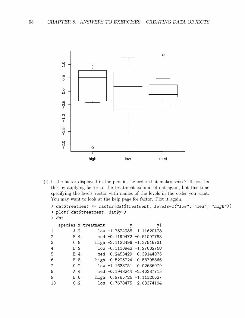
(i) Is the factor displayed in the plot in the order that makes sense? If not, fixthis by applying factor to the treatment column of dat again, but this timespecifying the levels vector with names of the levels in the order you want.You may want to look at the help page for factor. Plot it again.
> dat$treatment <- factor(dat$treatment, levels=c("low", "med", "high"))
> plot( dat$treatment, dat$y )
> dat
species x treatment y y1
1 A 2 low -1.7574988 1.11620178
2 B 4 med -0.1199472 -0.51097788
3 C 8 high -2.1122496 -1.27546731
4 D 2 low -0.3110942 -1.27632758
5 E 4 med -0.2453429 0.39144075
6 F 8 high 0.5225224 0.58795866
7 G 2 low -1.1633751 0.02636079
8 A 4 med -0.1948244 -2.40337715
9 B 8 high 0.9785726 -1.11326627
10 C 2 low 0.7678475 2.03374194

59
11 D 4 med 1.3574943 0.68305316
12 E 8 high -0.3029250 -0.73346041
13 F 2 low 0.6671354 2.54028332
14 G 4 med 0.0196097 1.09231928
15 A 8 high -0.4265499 0.89925111
16 B 2 low 0.1839618 -0.35779939
17 C 4 med 0.4749632 0.43452911
18 D 8 high 0.6700754 1.35573057
19 E 2 low 1.2702277 1.14789262
20 F 4 med -0.5149302 0.35294657
21 G 8 high 0.8784322 0.70047388
●
●
low med high
−2.
0−
1.5
−1.
0−
0.5
0.0
0.5
1.0
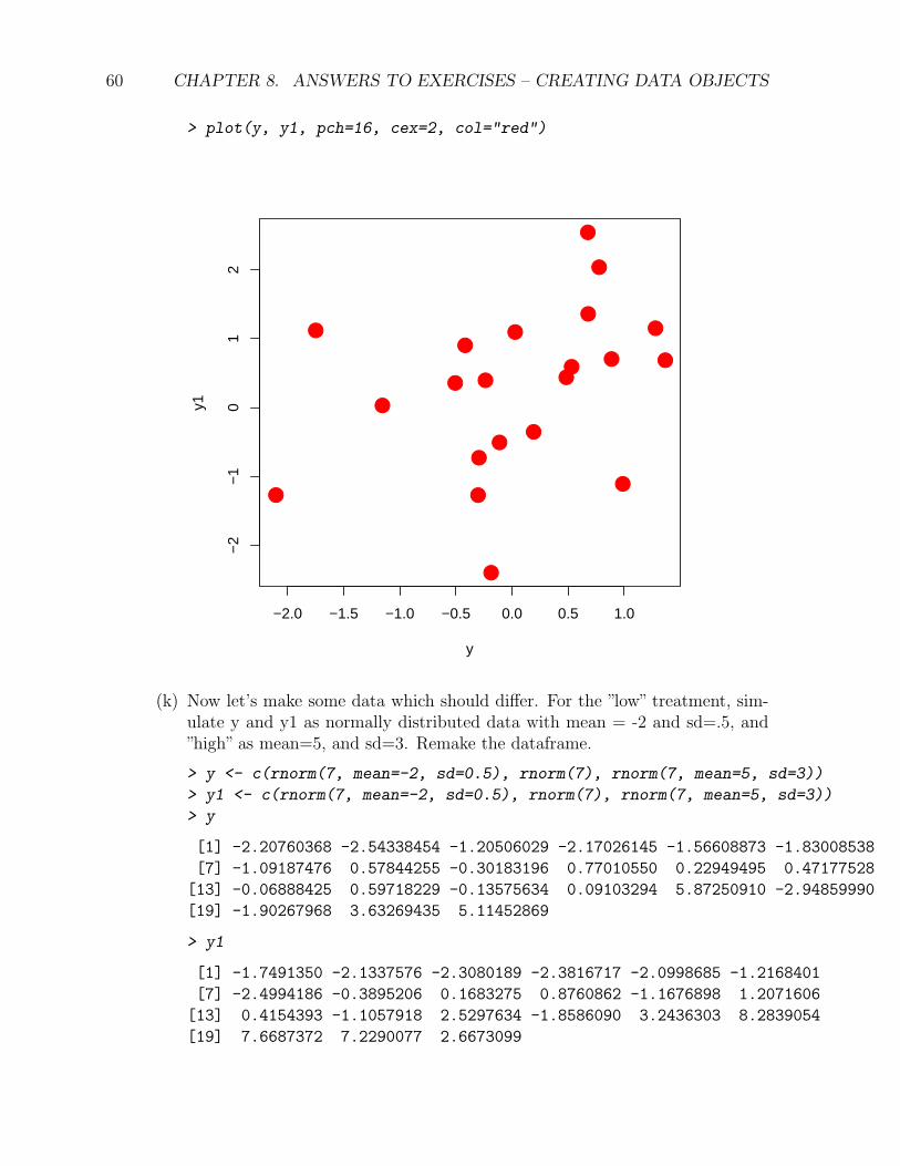
(j) Let’s make a scatterplot (plot(y, y1)) to see if there is any structuring in thedata (eventually with respect to the treatment levels – the rest of this exerciseis in the chapter on Workhorse Functions of Data Analysis). While we’re atit, let’s make it prettier. Change the symbols to solid circles by adding theoptional parameter pch=16, and the points bigger by cex=2. Change the colorto red using col="red".
60 CHAPTER 8. ANSWERS TO EXERCISES – CREATING DATA OBJECTS
> plot(y, y1, pch=16, cex=2, col="red")
●
●
● ●
●●
●
●
●
●
●
●
●
●●
●
●
●●
●
●
−2.0 −1.5 −1.0 −0.5 0.0 0.5 1.0
−2
−1
01
2
y
y1
(k) Now let’s make some data which should differ. For the ”low” treatment, sim-ulate y and y1 as normally distributed data with mean = -2 and sd=.5, and”high” as mean=5, and sd=3. Remake the dataframe.
> y <- c(rnorm(7, mean=-2, sd=0.5), rnorm(7), rnorm(7, mean=5, sd=3))
> y1 <- c(rnorm(7, mean=-2, sd=0.5), rnorm(7), rnorm(7, mean=5, sd=3))
> y
[1] -2.20760368 -2.54338454 -1.20506029 -2.17026145 -1.56608873 -1.83008538
[7] -1.09187476 0.57844255 -0.30183196 0.77010550 0.22949495 0.47177528
[13] -0.06888425 0.59718229 -0.13575634 0.09103294 5.87250910 -2.94859990
[19] -1.90267968 3.63269435 5.11452869
> y1
[1] -1.7491350 -2.1337576 -2.3080189 -2.3816717 -2.0998685 -1.2168401
[7] -2.4994186 -0.3895206 0.1683275 0.8760862 -1.1676898 1.2071606
[13] 0.4154393 -1.1057918 2.5297634 -1.8586090 3.2436303 8.2839054
[19] 7.6687372 7.2290077 2.6673099
61
> dat <- data.frame(species, x, treatment=factor(rep(c("low", "med",
+ "high"), each=7), levels=c("low", "med", "high")), y, y1)
> dat
species x treatment y y1
1 A 2 low -2.20760368 -1.7491350
2 B 4 low -2.54338454 -2.1337576
3 C 8 low -1.20506029 -2.3080189
4 D 2 low -2.17026145 -2.3816717
5 E 4 low -1.56608873 -2.0998685
6 F 8 low -1.83008538 -1.2168401
7 G 2 low -1.09187476 -2.4994186
8 A 4 med 0.57844255 -0.3895206
9 B 8 med -0.30183196 0.1683275
10 C 2 med 0.77010550 0.8760862
11 D 4 med 0.22949495 -1.1676898
12 E 8 med 0.47177528 1.2071606
13 F 2 med -0.06888425 0.4154393
14 G 4 med 0.59718229 -1.1057918
15 A 8 high -0.13575634 2.5297634
16 B 2 high 0.09103294 -1.8586090
17 C 4 high 5.87250910 3.2436303
18 D 8 high -2.94859990 8.2839054
19 E 2 high -1.90267968 7.6687372
20 F 4 high 3.63269435 7.2290077
21 G 8 high 5.11452869 2.6673099
(l) Make boxplots of species vs. y and species vs. y1. Why would you make thisplot?
> plot(dat$species, dat$y) # differences among species?

62 CHAPTER 8. ANSWERS TO EXERCISES – CREATING DATA OBJECTS
A B C D E F G
−2
02
46
> plot(dat$species, dat$y1)

63
A B C D E F G
−2
02
46
8

64 CHAPTER 8. ANSWERS TO EXERCISES – CREATING DATA OBJECTS
Chapter 9
Answers to Exercises – TheWorkhorse Functions of DataManipulation
Practice
1. Recall from the chapter on Data Objects that we were simulating data in differenttreatment groups, and wanting to visualize the groups. Now that we know how toindex and subset, we can use the points function to add different colored pointsto the plot for different groups.
(a) Now let’s make some data which should differ. For the ”low” treatment, sim-ulate y and y1 as normally distributed data with mean = -2 and sd=.5, and”high” as mean=5, and sd=3. Remake the dataframe.
> species <- LETTERS[1:7]
> x <- c(2, 4, 8)
> y <- c(rnorm(7, mean = -2, sd = 0.5), rnorm(7), rnorm(7, mean = 5,
+ sd = 3))
> y1 <- c(rnorm(7, mean = -2, sd = 0.5), rnorm(7), rnorm(7, mean = 5,
+ sd = 3))
> y
[1] -1.35675394 -1.46002699 -2.97437956 -2.18195253 -2.72455154 -1.60235344
[7] -2.50200360 1.12858736 0.73509477 -0.15948272 1.66442122 -1.37169030
[13] 0.09609262 -0.10948694 2.03646854 6.69888200 5.74442067 8.09971961
[19] 6.15534875 4.37892364 5.97545546
> y1
[1] -2.42076049 -1.51596326 -1.52024050 -2.30983016 -2.37689520 -1.33921323
[7] -2.12997281 -0.49157798 0.19920633 1.12167133 0.76742601 2.07451391
65
66CHAPTER 9. ANSWERS TO EXERCISES – THE WORKHORSE FUNCTIONS OF DATA MANIPULATION
[13] 0.85178268 0.16491571 4.73632224 5.14559468 2.26653806 2.90563718
[19] 0.03876202 11.95275699 2.47948626
> dat <- data.frame(species, x, treatment = factor(rep(c("low",
+ "med", "high"), each = 7), levels = c("low", "med", "high")),
+ y, y1)
> dat
species x treatment y y1
1 A 2 low -1.35675394 -2.42076049
2 B 4 low -1.46002699 -1.51596326
3 C 8 low -2.97437956 -1.52024050
4 D 2 low -2.18195253 -2.30983016
5 E 4 low -2.72455154 -2.37689520
6 F 8 low -1.60235344 -1.33921323
7 G 2 low -2.50200360 -2.12997281
8 A 4 med 1.12858736 -0.49157798
9 B 8 med 0.73509477 0.19920633
10 C 2 med -0.15948272 1.12167133
11 D 4 med 1.66442122 0.76742601
12 E 8 med -1.37169030 2.07451391
13 F 2 med 0.09609262 0.85178268
14 G 4 med -0.10948694 0.16491571
15 A 8 high 2.03646854 4.73632224
16 B 2 high 6.69888200 5.14559468
17 C 4 high 5.74442067 2.26653806
18 D 8 high 8.09971961 2.90563718
19 E 2 high 6.15534875 0.03876202
20 F 4 high 4.37892364 11.95275699
21 G 8 high 5.97545546 2.47948626
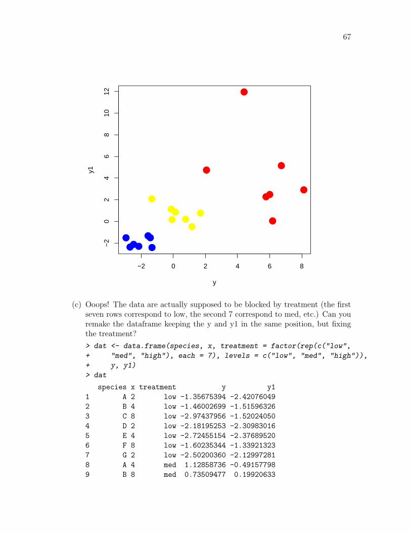
(b) Let’s differentially color the “high”, “medium”, and “low” points. First set upthe plot window without any points by plotting y, y1 with the plot parametertype="n". Then select only the ”high” points by subsetting. You’ll wantto make an index vector to choose only the points you want. Then use thepoints() function (which has the same form as the plot() function, butonly adds points to an existing plot. Choose three different colors for eachtreatment level and plot all the data. Is there any patterning in y, y1?
> plot(y, y1, type = "n")
> points(y[dat$treatment == "high"], y1[dat$treatment == "high"],
+ pch = 16, cex = 2, col = "red")
> points(y[dat$treatment == "med"], y1[dat$treatment == "med"],
+ pch = 16, cex = 2, col = "yellow")
> points(y[dat$treatment == "low"], y1[dat$treatment == "low"],
+ pch = 16, cex = 2, col = "blue")
67
−2 0 2 4 6 8
−2
02
46
810
12
y
y1 ●●
●●
●
●
●
●●
● ●
●
●●
●●●
●●
●●
(c) Ooops! The data are actually supposed to be blocked by treatment (the firstseven rows correspond to low, the second 7 correspond to med, etc.) Can youremake the dataframe keeping the y and y1 in the same position, but fixingthe treatment?
> dat <- data.frame(species, x, treatment = factor(rep(c("low",
+ "med", "high"), each = 7), levels = c("low", "med", "high")),
+ y, y1)
> dat
species x treatment y y1
1 A 2 low -1.35675394 -2.42076049
2 B 4 low -1.46002699 -1.51596326
3 C 8 low -2.97437956 -1.52024050
4 D 2 low -2.18195253 -2.30983016
5 E 4 low -2.72455154 -2.37689520
6 F 8 low -1.60235344 -1.33921323
7 G 2 low -2.50200360 -2.12997281
8 A 4 med 1.12858736 -0.49157798
9 B 8 med 0.73509477 0.19920633

68CHAPTER 9. ANSWERS TO EXERCISES – THE WORKHORSE FUNCTIONS OF DATA MANIPULATION
10 C 2 med -0.15948272 1.12167133
11 D 4 med 1.66442122 0.76742601
12 E 8 med -1.37169030 2.07451391
13 F 2 med 0.09609262 0.85178268
14 G 4 med -0.10948694 0.16491571
15 A 8 high 2.03646854 4.73632224
16 B 2 high 6.69888200 5.14559468
17 C 4 high 5.74442067 2.26653806
18 D 8 high 8.09971961 2.90563718
19 E 2 high 6.15534875 0.03876202
20 F 4 high 4.37892364 11.95275699
21 G 8 high 5.97545546 2.47948626
(d) Make three plots: boxplot of treatment vs. y, treatment vs. y1, and three colorscatterplot of y vs. y1 (treatments should be indicated by different colors).
> plot(dat$treatment, dat$y)
●
low med high
−2
02
46
8
> plot(dat$treatment, dat$y1)

69
●
low med high
−2
02
46
810
12
> plot(y, y1, type = "n")
> points(y[dat$treatment == "high"], y1[dat$treatment == "high"],
+ pch = 16, cex = 2, col = "red")
> points(y[dat$treatment == "med"], y1[dat$treatment == "med"],
+ pch = 16, cex = 2, col = "yellow")
> points(y[dat$treatment == "low"], y1[dat$treatment == "low"],
+ pch = 16, cex = 2, col = "blue")

70CHAPTER 9. ANSWERS TO EXERCISES – THE WORKHORSE FUNCTIONS OF DATA MANIPULATION
−2 0 2 4 6 8
−2
02
46
810
12
y
y1 ●●
●●
●
●
●
●●
● ●
●
●●
●●●
●●
●●
2. Matrix reshaping and indexing
(a) Create a matrix with the values 1 through 20, filling four rows. Save it as “x”.
> x <- matrix(1:20, nrow = 4)
> x
[,1] [,2] [,3] [,4] [,5]
[1,] 1 5 9 13 17
[2,] 2 6 10 14 18
[3,] 3 7 11 15 19
[4,] 4 8 12 16 20
(b) What are the attributes of x?
> attributes(x)
$dim
[1] 4 5
(c) Change it to a matrix with 2 rows and 10 columns by changing its attribute.
71
> dim(x) <- c(2, 10)
> x
[,1] [,2] [,3] [,4] [,5] [,6] [,7] [,8] [,9] [,10]
[1,] 1 3 5 7 9 11 13 15 17 19
[2,] 2 4 6 8 10 12 14 16 18 20
(d) Change x to a vector.
> dim(x) <- NULL
> x
[1] 1 2 3 4 5 6 7 8 9 10 11 12 13 14 15 16 17 18 19 20
> as.vector(x)
[1] 1 2 3 4 5 6 7 8 9 10 11 12 13 14 15 16 17 18 19 20
(e) Change x to a matrix with four rows, this time filling it by rows rather thanby columns (you may want to check the help page).
> x <- matrix(x, nrow = 4, byrow = TRUE)
(f) Coerce x to a vector again. Is it in the same order as the previous vector?What does this tell you about R’s default behavior when flattening matricesto vector?
> dim(x) <- NULL
(g) Create the original x matrix again. Select only the 3rd row, 4th column. Whatis it?
> x <- matrix(1:20, nrow = 4)
> x[3, 4]
[1] 15
(h) Select rows 3 and 4, columns 4 and 5. Print it to the console by using theprint(x) function.
> print(x[3:4, 4:5])
[,1] [,2]
[1,] 15 19
[2,] 16 20
(i) Select the first and last rows, first and last columns. Print it.
> print(x[c(1, 4), c(1, 5)])
[,1] [,2]
[1,] 1 17
[2,] 4 20
> print(x[c(1, nrow(x)), c(1, ncol(x))])
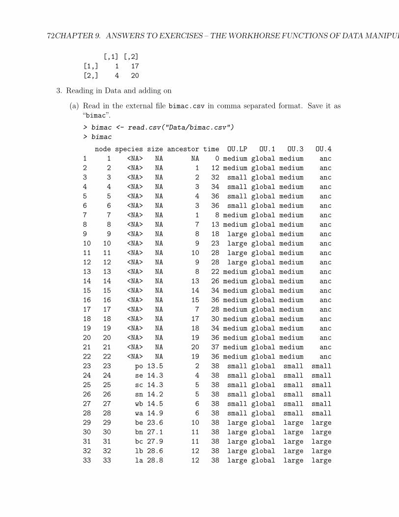
72CHAPTER 9. ANSWERS TO EXERCISES – THE WORKHORSE FUNCTIONS OF DATA MANIPULATION
[,1] [,2]
[1,] 1 17
[2,] 4 20
3. Reading in Data and adding on
(a) Read in the external file bimac.csv in comma separated format. Save it as“bimac”.
> bimac <- read.csv("Data/bimac.csv")
> bimac
node species size ancestor time OU.LP OU.1 OU.3 OU.4
1 1 <NA> NA NA 0 medium global medium anc
2 2 <NA> NA 1 12 medium global medium anc
3 3 <NA> NA 2 32 small global medium anc
4 4 <NA> NA 3 34 small global medium anc
5 5 <NA> NA 4 36 small global medium anc
6 6 <NA> NA 3 36 small global medium anc
7 7 <NA> NA 1 8 medium global medium anc
8 8 <NA> NA 7 13 medium global medium anc
9 9 <NA> NA 8 18 large global medium anc
10 10 <NA> NA 9 23 large global medium anc
11 11 <NA> NA 10 28 large global medium anc
12 12 <NA> NA 9 28 large global medium anc
13 13 <NA> NA 8 22 medium global medium anc
14 14 <NA> NA 13 26 medium global medium anc
15 15 <NA> NA 14 34 medium global medium anc
16 16 <NA> NA 15 36 medium global medium anc
17 17 <NA> NA 7 28 medium global medium anc
18 18 <NA> NA 17 30 medium global medium anc
19 19 <NA> NA 18 34 medium global medium anc
20 20 <NA> NA 19 36 medium global medium anc
21 21 <NA> NA 20 37 medium global medium anc
22 22 <NA> NA 19 36 medium global medium anc
23 23 po 13.5 2 38 small global small small
24 24 se 14.3 4 38 small global small small
25 25 sc 14.3 5 38 small global small small
26 26 sn 14.2 5 38 small global small small
27 27 wb 14.5 6 38 small global small small
28 28 wa 14.9 6 38 small global small small
29 29 be 23.6 10 38 large global large large
30 30 bn 27.1 11 38 large global large large
31 31 bc 27.9 11 38 large global large large
32 32 lb 28.6 12 38 large global large large
33 33 la 28.8 12 38 large global large large

73
34 34 nu 21.1 13 38 medium global medium medium
35 35 sa 18.3 14 38 medium global medium medium
36 36 gb 19.7 15 38 medium global medium medium
37 37 ga 18.8 16 38 medium global medium medium
38 38 gm 19.6 16 38 large global large large
39 39 oc 22.3 17 38 medium global medium medium
40 40 fe 28.4 18 38 medium global medium medium
41 41 li 18.7 20 38 medium global medium medium
42 42 mg 18.9 21 38 medium global medium medium
43 43 md 19.9 21 38 medium global medium medium
44 44 t1 21.3 22 38 medium global medium medium
45 45 t2 21.5 22 38 medium global medium medium
(b) This is a phylogenetic tree and data for the OUCH package. Without goinginto details for now, this method allows biologists to specify selective regimeson branches of the phylogeny, by specifying categories which correspond toalternative “niches”. This is a body size evolution dataset, and “OU.LP” is ahypothesis with three size categories. We would like to make three additionalhypotheses. Add additional columns to this dataframe: OU.1 which has valuesof “global” for all rows, OU.3 which is the same as OU.LP, except those rowswith “NA” in the species names should get a value of “medium”, and OU.4which is again similar to OU.LP, except that those rows with “NA” in thespecies names get a value of “anc”.
> bimac$OU.1 <- "global"
> bimac$OU.3 <- bimac$OU.LP
> bimac$OU.3[1:22] <- "medium"
> bimac$OU.3[is.na(bimac$species)] <- "medium"
> bimac$OU.4 <- as.character(bimac$OU.LP)
> bimac$OU.4[1:22] <- "anc"
> bimac$OU.4 <- factor(bimac$OU.4)
> bimac
node species size ancestor time OU.LP OU.1 OU.3 OU.4
1 1 <NA> NA NA 0 medium global medium anc
2 2 <NA> NA 1 12 medium global medium anc
3 3 <NA> NA 2 32 small global medium anc
4 4 <NA> NA 3 34 small global medium anc
5 5 <NA> NA 4 36 small global medium anc
6 6 <NA> NA 3 36 small global medium anc
7 7 <NA> NA 1 8 medium global medium anc
8 8 <NA> NA 7 13 medium global medium anc
9 9 <NA> NA 8 18 large global medium anc
10 10 <NA> NA 9 23 large global medium anc
11 11 <NA> NA 10 28 large global medium anc
12 12 <NA> NA 9 28 large global medium anc
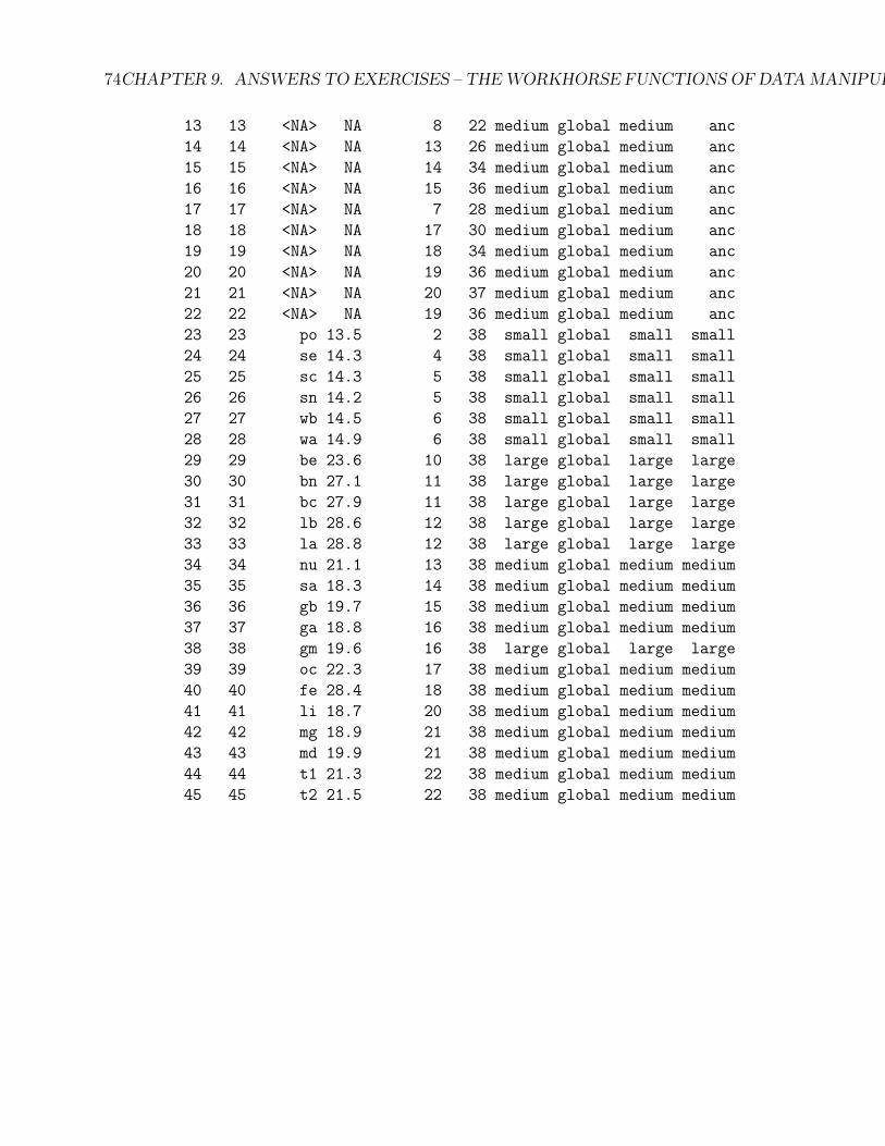
74CHAPTER 9. ANSWERS TO EXERCISES – THE WORKHORSE FUNCTIONS OF DATA MANIPULATION
13 13 <NA> NA 8 22 medium global medium anc
14 14 <NA> NA 13 26 medium global medium anc
15 15 <NA> NA 14 34 medium global medium anc
16 16 <NA> NA 15 36 medium global medium anc
17 17 <NA> NA 7 28 medium global medium anc
18 18 <NA> NA 17 30 medium global medium anc
19 19 <NA> NA 18 34 medium global medium anc
20 20 <NA> NA 19 36 medium global medium anc
21 21 <NA> NA 20 37 medium global medium anc
22 22 <NA> NA 19 36 medium global medium anc
23 23 po 13.5 2 38 small global small small
24 24 se 14.3 4 38 small global small small
25 25 sc 14.3 5 38 small global small small
26 26 sn 14.2 5 38 small global small small
27 27 wb 14.5 6 38 small global small small
28 28 wa 14.9 6 38 small global small small
29 29 be 23.6 10 38 large global large large
30 30 bn 27.1 11 38 large global large large
31 31 bc 27.9 11 38 large global large large
32 32 lb 28.6 12 38 large global large large
33 33 la 28.8 12 38 large global large large
34 34 nu 21.1 13 38 medium global medium medium
35 35 sa 18.3 14 38 medium global medium medium
36 36 gb 19.7 15 38 medium global medium medium
37 37 ga 18.8 16 38 medium global medium medium
38 38 gm 19.6 16 38 large global large large
39 39 oc 22.3 17 38 medium global medium medium
40 40 fe 28.4 18 38 medium global medium medium
41 41 li 18.7 20 38 medium global medium medium
42 42 mg 18.9 21 38 medium global medium medium
43 43 md 19.9 21 38 medium global medium medium
44 44 t1 21.3 22 38 medium global medium medium
45 45 t2 21.5 22 38 medium global medium medium