1

GIS Application in Water Balance

Modelling (Final paper)

By Hassan A. Eltoum

ID #240350

For

CRP 514: Introduction to GIS Term 051 – 12

th Offer

Course Instructor:

Dr. Baqer Al-Ramadan

Date 27, Dec, 2005

2

TABLE OF CONTENTS

Abstract 3

1- Introduction

……………………….. 5

2- Literature Review

……………………….. 6

3- Problem Statement

………………………... 6

4- Objectives

………………………… 7

5- Methodology

………………………… 7

5-1 Digital Elevation Map Processing

………………… 7

5-2 Selecting a Set of Flow Gages ………………. 10

5-3 Delineating Watersheds from Selected Gages ……. 10

5-4 Compiling Watershed Attributes ……………… 13

6- Discussion ………………………… 15

6-1 Atmospheric Water …………………………. 15

6-2 Soil Water …………………………. 17

6-3 Groundwater …………………………. 17

6-4 Surface Water …………………………. 18

6-5 Water Utilization …………………………. 19

7- Summary

…………………………. 21

References …………………………. 21

Appendix

22

3

ABSTRACT

The usage of GIS as a tool of water balance modeling is clearly seen in the literature; here

a lot of case studies were taken to come up with a clear, concise and brief report. The

whole budget of water balance could be subdivided into the flowing items: atmospheric

water balance, soil water balance, ground water balance, and surface water balance each

of these items has its own input and output. The most important step in the modelling of

water balance is the figuring out of the digital elevation map. (DEM) which help in assign

real direction of the water flow. By DEM along with aid of placing gages and setting of

watershed there will be a clear model for the area of interest. There are many papers

used in this report among which the most important one is that one come from Texas

University, it was used as a main reference.

4

1-INTRODUCTION

During the last decade there has been tremendous development in Hydrologic Modelling using

GIS. The use of digital terrain models has showed there were a potential number of analyses in

hydrology.

There are several possible applications of linking GIS with the hydrological models:

Hydrological Assessment to represent hazard or vulnerability (through weighted and

summed influences of significant factors rather than through physical laws)

Hydrological Parameter Determination, whereby the GIS provide inputs to the model in

terms of parameters such as surface slope, channel length, land use and soil characteristics.

Hydrological Modelling within the GIS, provides feasible time snapshots or temporal

averages are involved, not time – series.

Linking the GIS and hydrological model utilise the GIS as an input and display device,

including real time process monitoring if the necessary (remotely sensed) observations are

available.

However, the key factor to understand all of these aspects is rest on the understanding of water

balance which is define as a representation of the mass balance of water within a particular control

volume. It is a physical statement of the law of conservation of mass which states that matter

cannot be created or destroyed.(Daviad 1996)

The discussion will be briefly and short to give a general idea about how GIS could be an effective

tool special analysis of water balance. More over it will include the following items:

1- Atmospheric Water

2- Soil water

3- Ground water

4- Surface water

5- Water utilization

5

2- LITERATURE REVIEW

A number of researchers have used the atmospheric water balance to estimate hydrologic fluxes.

Among these researchers, Rasmusson, 1967, Brubaker et al., 1994, and Oki et al., 1995, describe

atmospheric water balance studies at river basin, continental, and global scales. Rasmusson, 1967,

analyzes the characteristics of total water vapor flux fields over North America and the Central

American Sea. A noteworthy observation made by Rasmusson is that a large diurnal wind system

covering the central United States, part of Mexico, and the Central American Sea produces

significant diurnal variations in the transport of water vapor. By decomposing the vertically

integrated vapor flux term into mean motion and transient eddy terms, where the mean motion

term is at a time scale of one month and the transient eddy term describes motion at a time scale of

less than one month, Brubaker et. al. also observe important vapor flux transport at sub-monthly

time scales. Brubaker et. al. note that poleward eddy flux transport from the Gulf of Mexico is

significant, particularly during the winter months. From these observations, Brubaker et. al.

surmise that the use of monthly-averaged or sparse data may significantly underestimate the eddy

flux component of vapor transport. These observations are relevant to the interpretation of our

results, as discussed in Section 3.3. Brubaker et al. also note that the accuracy of runoff estimates

made using atmospheric data increases with the size of the study area and cite a recommendation

by Rasmusson, 1977, that a minimum area of 106 km

2 should be used. The area of Texas is about

0.7 x 106 km

2. Improvements in observational networks and general circulation models may justify

runoff estimation on smaller areas in the future.

The Environmental Resource Management Division of the Environmental and Conservation

Services Department of the City of Austin (1995) has analyzed the storm water pollution and its

relation to the watershed development conditions. In this study, relations between pollutant

concentrations, impervious cover, runoff coefficients, etc. here the need of the water balance

modeling rise and it was one of the study items

6

3- PROBLEM STATMENT

There is a big demand for the special analysis of water recourses , surface water , contaminant ,

and waste water this demand reflect on the need of water balance modeling which will give a

better look to analysis any problem in water resources

4- OBJECTIVES

The objectives of this term paper are to :

(1) Elaborate on general idea for modeling water balance and,

(2) have a look to developing tools for predicting hydrographs and pollution, and to do this taking

into account the spatial of water balance. This mission will be accomplished by reviewing a lot of

published paper and come up with one coincide topic include all the discussion and

recommendation with appropriate methodology.

5- METHODS

There are many methodology in the publish literature for modeling water balance all of which,

used Arc view for special analysis. Each one will be described briefly to give an overview to the

resulting conclusion the most clear one is that described in project of Texas water balance which

include the fallowing major steps (1) DEM processing, (2) selecting a set of flow gages spanning

the appropriate period of record, (3) Compiling Watershed Attributes (4) determining the average

annual precipitation in each watershed, (5) determining the net measured inflow to each watershed,

(6) compiling a set of watershed attributes including percent urbanization, reservoir evaporation,

recharge, and spring flow, (7) plotting runoff per unit area versus rainfall per unit area and deriving

an "expected" runoff function, and (8) creating grids of expected runoff, actual runoff, and

evaporation.

7

5-1 Digital Elevation Map Processing:

Digital Elevation Models or DEMs are increasingly becoming the focus of attention within

the larger realm of digital topographic data. The quality and calibre if DEMs has been

extremely valuable in the hydrological applications. DEM provides a digital representation

of a portion of the earth’s terrain over a two dimensional surface (Figure1). DEM data are

available in the United States at 30m and 3" cell size, suitable for delineating watersheds and

stream networks within urban areas or in small river basins, at 15" cell size which is suitable for

regional studies of the size of Texas, to 30" cell size which is appropriate for continental scale

studies to 5' cell size covering the earth. The 30" DEM's for Africa and other regions being

constructed by Sue Jenson and her co-workers at the USGS using the Digital Chart of the World

are a significant contribution.

Delineation of watersheds from DEM data has become standardized on the eight-direction pour

point model in which each cell is connected to one of its eight neighbour cells (four on the

principal axes, four on the diagonals) according to the direction of steepest descent. Given an

elevation grid, a grid of flow directions is constructed, and from this is derived a grid of flow

accumulation, counting the number of cells upstream of a given cell. Streams are identified as lines

of cells whose flow accumulation exceeds a specified number of cells and thus a specified

upstream drainage area.

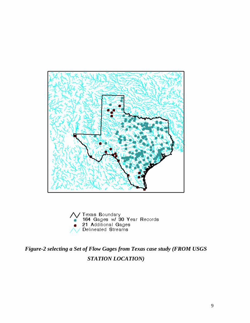
5-2 Selecting a Set of Flow Gages:

All monthly and daily flow records for the water certain years and for all USGS gaging stations in

specific place were extracted from the Hydrosphere CD-ROM "USGS Daily Values : West 2."

The Hydrosphere software is always used to write the flow records for all stations to a dBase file.

This dBase file also includes latitude, longitude, and other station information. Key attributes

available for each station record are latitude, longitude, starting year, ending year. Selecting asset

of flow gages is clearly seen in Texas water balance case study. Figure 2

8

Figure-1 Drainage Network Delineation (AFTER DAILY 1990)

9

Figure-2 selecting a Set of Flow Gages from Texas case study (FROM USGS

STATION LOCATION)

10

5-3 Delineating Watersheds from Selected Gages:

A standardized way of delineating watersheds and stream networks is the following:

1- Construct the stream network in the standard way by choosing a drainage area threshold;

2- Divide the stream network so created into individual stream links;

3- Find the outlet cell at the lower end of each link;

4- Delineate the watershed for each of these outlet cells.

By changing the threshold drainage area, sub watersheds can be delineated within watersheds in a

nicely scaled manner. This algorithm has a critical property - there is one and only one stream for

each watershed, which makes modeling of the flow of water from watersheds to the streams within

them feasible within GIS. Also, there is a one to one relation between the raster representation of

the landscape and the vector features of streams and watersheds derived from it.

5-4 Compiling Watershed Attributes:

There are many attribute that could be assigning to the watershed like:

1) Determining Mean Precipitation and Net Inflow, 2) Reservoir Evaporation, 3) Urban Land use,

4) Recharge 5) Springs

Each of these attribute has its important and significant and it is determined by long procedure

after determination of water shade.

11

Figure 3. Delineating Watersheds from Selected Gages(FROM TEXAS GROUP

OF GIS)

12

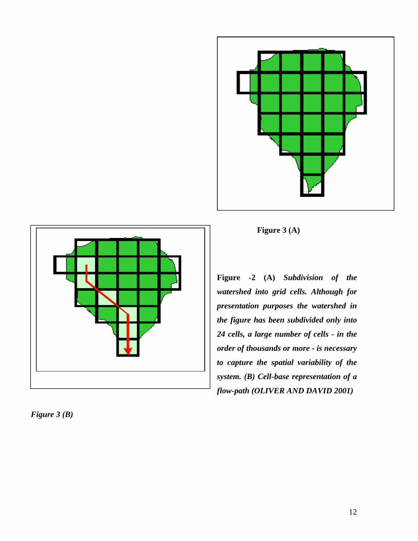
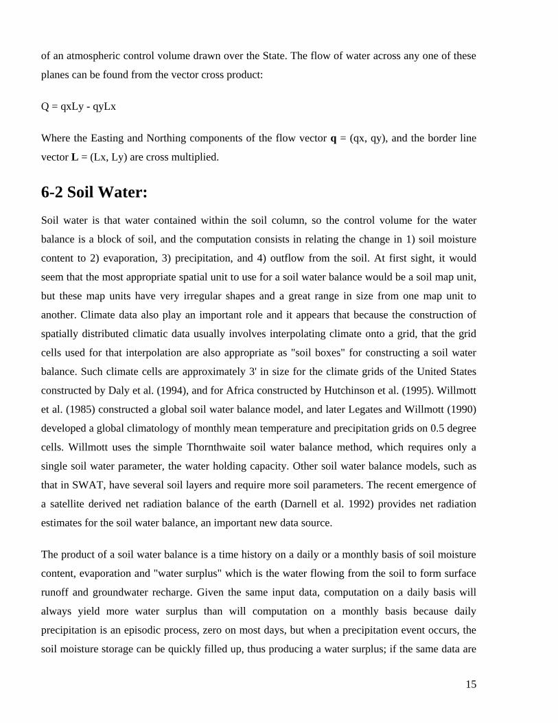
Figure 3 (A)

Figure -2 (A) Subdivision of the

watershed into grid cells. Although for

presentation purposes the watershed in

the figure has been subdivided only into

24 cells, a large number of cells - in the

order of thousands or more - is necessary

to capture the spatial variability of the

system. (B) Cell-base representation of a

flow-path (OLIVER AND DAVID 2001)

Figure 3 (B)

13

6- DISCUSSION

As a discussion here all results and methodology from review paper will be combined together for

the purpose of comparison. It is found that the use of GIS in the modeling water balance is a very

valuable tool that gives a better look to the water budget. For this purpose water budget is

classified to many domain each of which with its one parameters and individual small scale

budget. Those are: Atmospheric Water, Soil water, Ground water, Surface water, Water utilization

6-1 Atmospheric Water:

The first step to examine water balance is to examine the most water that falls on the land surface

which is derived from oceanic evaporation carried inland by atmospheric circulation, so it is

appropriate to begin the study of water by examining the motion of atmospheric water. The most

useful way of doing this in a GIS context is to use the results of GCM modeling, where the

acronym GCM means here General Circulation Model. The condition of the atmosphere

(temperature, density, wind velocity, air pressure, and moisture content) is calculated on a

geographic grid of 2 degree cells covering the earth, using a very short time interval of the order of

a few minutes, for a time horizon of a few days ahead. Each 12 hours, the forecasts are updated

with new observations, and the process repeated. Figure 4 shows how the expression of the

atmospheric modeling would be.

With atmospheric moisture flow being given by the product of the wind velocity and atmospheric

moisture content, vertically integrated over the height of the atmosphere, spatially averaged over

the 2 degree grid, and time averaged over a month,. An animation of these data, shows that the

bulk of the water precipitating over the central and eastern regions of any area is derived from

evaporation in the adjacent Sea

The atmospheric water balance for a region can be computed by taking the vector field of

atmospheric moisture flow, q, defined on the 2 degree grid, and interpolating the flow vectors onto

points lying on the border of the region at regular intervals. . The lines joining these border points

are also a set of vectors, L, which can be imagined to project vertically into the atmosphere and

form a closed set of planes surrounding the atmosphere of the State, which are the control surface

14

Figure4. A) (Up left) Degree Cells Overlaid on a region. B) (Up right) Computational Cells

Intersected with the Generalized certain region. C) How Moisture Flux Vectors appear in a

certain time.(TEXAS GROUP OF GIS)

15

of an atmospheric control volume drawn over the State. The flow of water across any one of these

planes can be found from the vector cross product:

Q = qxLy - qyLx

Where the Easting and Northing components of the flow vector q = (qx, qy), and the border line

vector L = (Lx, Ly) are cross multiplied.

6-2 Soil Water:

Soil water is that water contained within the soil column, so the control volume for the water

balance is a block of soil, and the computation consists in relating the change in 1) soil moisture

content to 2) evaporation, 3) precipitation, and 4) outflow from the soil. At first sight, it would

seem that the most appropriate spatial unit to use for a soil water balance would be a soil map unit,

but these map units have very irregular shapes and a great range in size from one map unit to

another. Climate data also play an important role and it appears that because the construction of

spatially distributed climatic data usually involves interpolating climate onto a grid, that the grid

cells used for that interpolation are also appropriate as "soil boxes" for constructing a soil water

balance. Such climate cells are approximately 3' in size for the climate grids of the United States

constructed by Daly et al. (1994), and for Africa constructed by Hutchinson et al. (1995). Willmott

et al. (1985) constructed a global soil water balance model, and later Legates and Willmott (1990)

developed a global climatology of monthly mean temperature and precipitation grids on 0.5 degree

cells. Willmott uses the simple Thornthwaite soil water balance method, which requires only a

single soil water parameter, the water holding capacity. Other soil water balance models, such as

that in SWAT, have several soil layers and require more soil parameters. The recent emergence of

a satellite derived net radiation balance of the earth (Darnell et al. 1992) provides net radiation

estimates for the soil water balance, an important new data source.

The product of a soil water balance is a time history on a daily or a monthly basis of soil moisture

content, evaporation and "water surplus" which is the water flowing from the soil to form surface

runoff and groundwater recharge. Given the same input data, computation on a daily basis will

always yield more water surplus than will computation on a monthly basis because daily

precipitation is an episodic process, zero on most days, but when a precipitation event occurs, the

soil moisture storage can be quickly filled up, thus producing a water surplus; if the same data are

16

averaged over a monthly interval, it is as if the precipitation falls as a gentle mist, which may

evaporate back to the atmosphere before the soil moisture capacity is filled. Interpolation of daily

precipitation onto a grid is an uncertain undertaking because the spatial variation in daily

precipitation is large. There is thus a challenge in constructing a GIS hydrology model for soil

water balance in choosing the appropriate time interval for calculation.

6-3 Groundwater:

There are two kinds of groundwater flow: unconfined flow, which occurs near the land surface and

for which the water table or phreatic surface is the upper boundary of the saturated aquifer, and

confined flow which occurs in deeper aquifers where the upper boundary on the flow is provided

by an overlying hydro geologic unit of low permeability. Unconfined flow is strongly influenced

by surface hydrologic conditions, especially by seepage from streams crossing the region where

the aquifer outcrops at the land surface. Confined flow is less influenced by surface conditions.

Groundwater flow models usually use rectangular or triangular spatial units to represent

elementary volumes of porous medium upon which the computations are to be performed. A GIS-

based groundwater model can similarly be constructed using polygonal units provided the

polygons are reasonably regularly shaped, but groundwater models constructed within GIS are not

very computationally efficient.

In constructing a groundwater balance model, there are two computations to be performed: first, a

water balance on each spatial unit in which all the inflows and outflows of the unit are used to

determine the change in water storage and thus of the piezometric head within the unit; second, a

flow computation between each pair of spatial units in which Darcy's law is used to determine the

rate of groundwater flow as a function of the difference in head and the flow properties of the

aquifer in the units. In a map-based groundwater modeling system, the first computation is done

over all the polygons making up the aquifer, while the second is done over all the boundary lines

of those polygons. Interaction between surface water in streams and underlying groundwater can

be similarly determined by applying Darcy's law to the difference in piezometric head between the

stream passing through an aquifer unit and the surrounding aquifer. All these computations need to

be done on reasonably small units not more than say 20 km in cell size, because otherwise the head

17

gradients in space become very small. Groundwater aquifers are usually quite confined in area and

do not extend over the whole landscape, so unlike surface water flow which takes place

everywhere, groundwater flow is more of a localized problem and a regional study needs to take

into account each aquifer in the region individually, rather than considering groundwater flow to

be a regional phenomenon.

6-4 Surface Water:

Surface water is water in streams, lakes, wetlands and reservoirs. This water system is in some

ways the most complex of all the phases of the hydrologic cycle, because it interacts with the other

three phases, namely atmospheric water, soil water and groundwater, because the flow velocity is

large compared to the velocity of groundwater flow, and because the flow environment is

complicated, depending in part on the characteristics of the land surface and in part on the

characteristics of the stream system. Fortunately, this is the area where GIS helps the most because

of the detailed description of land surface features which can be presented in GIS. As described

earlier, by making a suitable terrain analysis using DEM data, a conceptual model of the surface

drainage system can be built up in which each watershed has one and only one stream draining it,

and each watershed and stream pair can be assigned the same identification number. The

watersheds so constructed are of two types: a source or head watershed in which the stream

originates within the watershed, and an intermediate watershed where the stream flows both into

and out of the watershed.

The stream network is manipulated so that each stream is represented by a single arc, and the arcs

are flow ordered so that the from node is upstream and the to node is down stream. Each stream

arc is enclosed within its associated watershed polygon. Watershed boundaries are delineated from

each stream junction so at most a node can have two streams flowing into it and one flowing out of

it. Three flow variables can be associated with each watershed: "From Flow", "To Flow", and

"Polygon Flow". From Flow is that stream discharge at the from node; To Flow is the

corresponding discharge at the to node; and Polygon Flow is that discharge which comes into the

stream by drainage from the surrounding watershed. Polygon Flow is computed by applying a unit

hydrograph to the water surplus computed by the soil water balance model, and it may also include

a component representing exchange of water between the stream and the underlying groundwater

18

aquifer. This implies that the soil water surplus data may have to be spatially transferred from the

soil water balance spatial units to the watershed units by using polygon overlay functions. The

Polygon Flow can be divided by the length of the stream and added progressively to the discharge

along the path of the stream, so in a time-averaged calculation, the discharge at a distance D from

the upstream end of a stream of length L is given by:

Discharge = From Flow + (Polygon Flow / L) * D

In time-varying flow, the computation is more complex and stream routing methods such as the

Muskingum method (Fread, 1993) are appropriate for computing the time distribution of the To

Flow given the time distribution of the From Flow and the Polygon Flow. The time table structure

described earlier in the paper is used to record the results of these calculations with a separate table

being used for each of the three flow variables, a separate field for each watershed, and time on the

vertical axis of the table.

In doing such computations, there is a choice between sequencing the computations "first in space

and then in time" or "first in time and then in space", in other words, doing all the computations for

a given watershed through time and then moving to the next watershed, or doing the computations

for all watersheds for one time interval before moving to the next time interval. For regional

hydrologic studies where the watersheds don't influence one another the "first in space then in

time" method works best; for more localized hydraulic analyses where water level in the river

influences groundwater levels, the simultaneous nature of the interactions makes the "first in time

then in space" method necessary. The nature of the process interactions governs the computational

sequence.

6-5 Water Utilization:

All of the preceding discussion is valid for a pristine landscape untouched by human activity. But

reservoir construction, pumping of water from rivers and groundwater systems, and discharge of

wastewater all has profound effects on surface and groundwater flow and quality. Modeling the

effects of water utilization permits GIS hydrology models to be useful as a basis for planning

decisions on water facilities. Consider a pumping station withdrawing water from a river. In a

spatial sense, this can be represented by a point on a river with attributes describing the time

19

pattern of withdrawals. It is useful to locate this point by its relative distance from the upstream

end of the reach (D/L in the nomenclature defined previously). This "proportional aliasing"

provides a way of locating objects on river reaches which is somewhat independent of the scale of

the map used to define the river reach spatially. River reaches are always longer on maps of larger

scale but the relative location of a point remains reasonably stable across scales. Once the

withdrawal is located, it can be included in the discharge computation.

Including reservoirs in the computation is more complicated because a reservoir is a fairly

complicated system by itself, and its outflow depends on the manner in which the reservoir control

works are operated. A standard method of simulating water supply reservoirs is presented by

Chow, Maidment and Mays (1988).

7- SUMMARY

To facilitate the surface water balance, gaging stations were selected for analysis, and a digital

elevation model was used to delineate the drainage areas for each gage. A grid of mean annual

precipitation and mean annual runoff values compiled for each gage were used to derive a

relationship between mean annual precipitation (mm) and the mean annual surface runoff (mm).

and applies in areas without unusually large groundwater recharge, spring flow, urbanization, or

reservoir impoundment. Applying this relationship to the precipitation grid, a grid of expected

runoff was derived.

Many water balance methods - an atmospheric water balance, a soil-water balance, and a surface

water balance - have been used in an attempt to gain an improved understanding of the stocks of

water in different components of the hydrologic cycle and the fluxes between these components.

Given adequate data, the atmospheric water balance is a promising method for estimating regional

evaporation, runoff, and changes in basin storage; however, Estimates of mean annual divergence

over any area were made using both observed raw data and the output data from a general

circulation model.

20

The soil-water balance is a climatological approach which is instructive, but also contains

substantial uncertainties. The main reasons for the uncertainties in the soil-water balance are a

simplified representation of land surface hydrology, the use of monthly average rainfall data, and

the fact that there is no calibration with observed data of either soil moisture or runoff. Because of

these assumptions, the soil-water balance model predicts zero runoff over large areas of the State

where surface runoff actually does occur. The soil-water balance does provide qualitative

information about the space and time variability of soil moisture and evapo-transpiration that are

not revealed by the annual surface water balance, but a way to confirm these results has not been

worked out.

8- CONCLUSIONS

Three water balance methods - an atmospheric water balance, a soil-water balance, and a surface

water balance - have been used in an attempt to gain an improved understanding of the stocks of

water in different components of the hydrologic cycle and the fluxes between these components.

Given adequate data, the atmospheric water balance is a promising method for estimating regional

evaporation, runoff, and changes in basin storage; however if, data used in this study were not at a

high enough resolution to make accurate calculations for any region the estimate of mean annual

divergence over the it were made using both observed rawinsonde data and the output data from a

general circulation model.

The soil-water balance is a climatological approach which is instructive, but also contains

substantial uncertainties. The main reasons for the uncertainties in the soil-water balance are a

simplified representation of land surface hydrology, the use of monthly average rainfall data, and

the fact that there is no calibration with observed data of either soil moisture or runoff. Because of

these assumptions, the soil-water balance model predicts zero runoff over large areas of the region

surface runoff actually does occur. The soil-water balance does provide qualitative information

about the space and time variability of soil moisture and evapotranspiration that are not revealed

by the annual surface water balance, but a way to confirm these results has not been worked out.

21

A grid of mean annual expected evaporation could be estimated by subtracting the grid of expected

runoff from the precipitation grid. The values of expected evaporation range from 200 mm year-.

Using the evaporation grid, the net radiation grid, and a temperature grid, a map of mean annual

Bowen ratios for any region was created. These Bowen ratio values vary from from place to place

according to all water balance parameters .

8- RECOMMENDATIONS

As spatial data sets from remote sensing continue to improve along with tools like a GIS for

manipulating spatial data, hydrologists can think in terms of water maps both in the atmosphere

and on the land surface rather than thinking just in terms of point measurements Huns the use of

remote sensing is corner stone in this type of research .

Working with a GIS allows for the computation of water balances on arbitrary control volumes and

simplifies the use of complex spatial data. There for alarge amount of data for the state of region

will be useful to others in the future.

22

References

1. Alley, W.M., "On The Treatment Of Evapotranspiration, Soil Moisture Accounting, and

Aquifer Recharge in Monthly Water Balance Models," Water Resources Research, 20,1137-

1149,1984

2. Arnell, N.W., "Grid Mapping of River Discharge," Journal of Hydrology, 167, 39-56, 1995.

3. ASCE, Evapotranspiration and Irrigation Water Requirements, Jensen, M.E., R.D. Burman,

and R.G. Allen (editors), ASCE Manuals and Reports on Engineering Practice No. 70, 1990.

4. Atkinson, S.F., J.R. Thomlinson, B.A. Hunter, J.M. Coffey, and K.L. Dickson, "The

DRASTIC Groundwater Pollution Potential of Texas," prepared by The Center for Remote

Sensing and Landuse Analyses Institute of Applied Sciences, University of North Texas,

Denton, Texas, September, 1992.

5. Atkinson, S.F., J.R. Thomlinson, "An Examination of Ground Water Pollution Potential

Through GIS Modeling," ASPRS/ACSM Annual Convention and Exposition : Technical

Papers, Reno, Nevada, 1994.

6. Brubaker, K.L., D. Entekhabi, and P.S. Eagleson, "Atmospheric Water Vapor Transport and

Continental Hydrology over the Americas," Journal of Hydrology, 155, 407-428, 1994.

7. Brutsaert, W., Evaporation into the Atmosphere: Theory, History, and Applications, D.

Reidel Publishing Company, Dordrecht, Holland, 1982.

8. Chow, V.T., D.R. Maidment, and L.W. Mays, Applied Hydrology, McGraw-Hill, Inc., New

York, NY, 1988.

9. Church, M. R., G.D. Bishop, and D.L. Cassell, "Maps of Regional Evapotranspiration and

Runoff/Precipitation Ratios in the Northeast United States," Journal of Hydrology, 168, 283-

298, 1995.

10. Daly, C., R. Neilson, and D. Phillips, "A Statistical-Topographic Model for Mapping

Climatological Precipitation over Mountainous Terrain," Journal of Applied Meteorology ,

33, 2, February 1994.

11. Darnell, W.L., W.F. Staylor, S.K. Gupta, N.A. Ritchey, and A.C. Wilber, "Seasonal

Variation of Surface Radiation Budget Derived from ISCCP-C1 Data," J. Geophysical. Res.,

97, 15741-15760, 1992.

23

12. Darnell, W.L., W.F. Staylor, S.K. Gupta, N.A. Ritchey, and A.C. Wilber, "A Global Long-

term Data Set of Shortwave and Longwave Surface Radiation Budget," GEWEX News, 5,

No.3, August 1995.

13. Dingman, S.L., Physical Hydrology, Prentice Hall, Inc., Englewood Cliffs, NJ, 1994.

14. Dugas, W.A., and C.G. Ainsworth, Agroclimatic Atlas of Texas, Part 6: Potential

Evapotranspiration, Report MP 1543, Texas Agricultural Experiment Station, College

Station, December, 1983.

15. Dyck, S., "Overview on the Present Status of the Concepts of Water Balance Models," New

Approaches in Water Balance Computations (Proceedings of the Hamburg Workshop),

IAHS Publ. No. 148, 1983.

16. Dunne, K.A., and C.J. Willmott, "Global Distribution of Plant-extractable Water Capacity of

Soil," International Journal of Climatology, 16, 841-859, 1996.

17. "Global Energy and Water Cycle Experiment (GEWEX) News," World Climate Research

Programme, August, 1995, V. 5, No. 3.

18. Gutman, G., and L. Rukhovetz, "Towards Satellite-Derived Global Estimation of Monthly

Evapotranspiration Over Land Surfaces," Adv. Space Res., 18, No. 7, 67-71, 1996.

19. Hydrodata CD-ROM, "NCDC Summary of the Day - West 2," Hydrosphere, Boulder, CO,

1994.

20. Hydrodata CD-ROM, "USGS Daily Values - West 2," Hydrosphere, Boulder, CO, 1994.

21. Kreyszig, E., Advanced Engineering Mathematics, 7th

Edition, John Wiley and Sons, Inc.,

1993.

22. Legates, D.R., and Willmott, C.J., "Mean Seasonal and Spatial Variability in Gauge-

Corrected, Global Precipitation," International Journal of Climatology, 10, 111-127, 1990.

23. Lullwitz, T. and A. Helbig, "Grid Related Estimates of Streamflow within the Weser River

Basin, Germany," Modeling and Management of Sustainable Basin-scale Water Resource

Systems, Symposium Proceedings, Boulder, Colorado, IAHS Publ. No. 231, 1995.

24. Maidment, D.R., "GIS and Hydrologic Modeling - an Assessment of Progress,"

http://www.ce.utexas.edu/prof/maidment/GISHydro/meetings/santafe/santafe.html.