gis-modelling of potential natural vegetation (pnv): a
TRANSCRIPT

GIS-modelling of potential natural vegetation
(PNV): A methodological case study from
south-central Norway
GIS-modellering av potensiell naturleg vegetasjon
(PNV): Eit metode studie frå sentrale Sør-Noreg
Lars Østbye Hemsing
Departmentofecologyandnaturalresourcemanagement
MasterThesis30credits2010


I
Preface
-
project: 189977), initiated by The Norwegian Forest and Landscape Institute (TNFLI) and the
Norwegian Hospitality Association and with financial support from The Research Council of
Norway, as well as other partners. TNFLI provided me with financial support and has been a
collaborating partner during the course of my work on this project.
I would like to thank my supervisor Terje Gobakken for helpful and constructive comments.
Special thanks are also due to my secondary supervisor Dr Anders Bryn, who has provided
support and good advice throughout the whole writing process. He deserves special thanks for
assisting me with the vegetation mapping during the summer of 2009.
In additi -
Oslo for allowing me to participate in their internal Maxent seminar. Finn-Arne Haugen also
deserves thanks for reviewing the manuscript and for valuable discussion on the mapping of
PNVE prior to the mapping of my study area. I would also like to thank Catriona Turner for
helping me with correcting the language.
I am especially grateful to my girlfriend, Elisabeth, for being patient and supporting me
throughout the time spent in connection with this study.
Norwegian University of Life Sciences
Ås, 15. May 2010
______________________________
Lars Østbye Hemsing


III
Summary
Potential natural vegetation (PNV) is a hypothetic natural state of vegetation that shows
PNV with actual vegetation, anthropogenic influences can be assessed and quantified. Actual
vegetation in a mid-south Norwegian mountain region, located around the village of
Beitostølen in Valdres, was mapped during fieldwork in summer 2009. This vegetation map
formed the basis for the development of PNV using three different modelling methods. The
purpose was to explore the different methods and attempt to locate anthropogenic
disturbances. The first method was based on an expert-valuated manual mapped PNV map
(PNVE) created simultaneously while mapping actual vegetation. The second model was
created as a rule-based envelope GIS model (RBM), while the third model was created with a
statistical predictive GIS modelling method, Maxent. RMB and Maxent were created with a
basis in actual vegetation in addition to environmental predictor variables.
All models predicted the same vegetation types for 61% of total area, while different
vegetation types were only predicted for 2% of total area. PNVE and Maxent were the two
methods with highest accordance (87% of total area). Differences among modelling outputs
were related to determine the upper potential forest limit for dominating tree species (birch
and spruce), to model PNV for areas which are moderately to heavily disturbed by humans
(e.g. farmland, housing estates, drained forests/swamps), and to model vegetation types that
occur in their ecological extremities (e.g. humid types, rich types, successional state). The
general tendencies for all three PNV models show a considerable increase and elevation of
spruce forest, with a stable amount of birch forest, and decreasing amounts of boreal heath
and meadow communities. Areas with boreal heath and meadow communities are
transformed into mountain birch forest, whereas birch forest at lower altitudes is transformed
into spruce forest.
PNV maps and actual vegetation maps were compared to reveal traces of earlier human
disturbance; areas where vegetation types differed were considered as anthropogenically
disturbed. All models predicted that more than 50% of vegetation from the actual vegetation
map would be prevented from reaching its biotic potential. PNVE was the only model which
captured human disturbance above the upper potential forest limit in the PNV maps. Shifts in
forest distribution are known to be one of the major consequences of land-use changes in
mountain areas.

V
Samandrag
Potensiell naturleg vegetasjon (PNV) er ein hypotetisk naturleg tilstand som vegetasjon syner
naturens biotiske potensiale, forutsett at menneskeleg påverknad og forstyrring aldri har funne
stad. Ved å samanlikne PNV og aktuell vegetasjon kan menneskeleg påverknad verta kartfesta
og kvantifisert. Aktuell vegetasjonen vart kartlagt gjennom feltarbeid sommaren 2009. Dette
vegetasjonskartet danna grunnlaget for seinare utvikling av PNV kart ved hjelp av tre ulike
tilnærmingar for ein sentral Sør-Norsk fjellregion, lokalisert rundt Beitostølen i Valdres.
Hensikta var å undersøkje ulike tilnærmingar, og forsøkje å kartfesta menneskeskapte
forstyrringar av naturen. Første tilnærming er basert på eit ekspert evaluert, manuell kartlagt
PNV kart (PNVE) som vart danna fortløpande med kartlegging av aktuell vegetasjon. Den
andre tilnærminga er danna som ein regelstyrt konvolutt-modell (RBM) i GIS, medan den
tredje tilnærminga er oppretta med ein statistisk prediktiv GIS-modellerings metode, Maxent.
Dei to GIS-modellane vart danna på grunnlag av aktuell vegetasjon og miljøvariablar.
Alle tilnærmingane predikerte same vegetasjonstyper for 61% av det totale areal, medan berre
2% av totalt areal vart predikert med ulike vegetasjonstypar. PNVE og Maxent var dei to
tilnærmingane med høgast samsvar (total 87% av areal). Skilnadar mellom
tilnærmingsmåtane var knytta til fastsetjing av øvre potensielle skoggrense for dominerende
treslag (bjørk og gran), til å lage PNV for område som er moderat til sterkt forstyrra av
menneskeleg endringar (t.d. jordbruksområder, boligfelt, drenerte skogar/myrar) og til å
predikera vegetasjonstypar som førekjem i deira økologiske ytterpunkt (t.d fuktige typar, rike
typar, ulike suksesjonsstadium). Generelle trendar for alle PNV tilnærmingane syner ei
tydeleg auke i mengd og auke av granskogen, med stabil arealmessig mengde bjørkeskog, og
ein betydeleg reduksjon av boreale lyngheiear, og boreale engsamfunn. Område med boreale
lyngheiar og engamfunn blir omdanna til fjellbjørkeskog, medan bjørkeskogen ved lågare
høgder vert omdanna til granskog.
PNV kart og aktuellt vegetasjonskart vart samanlikna for å avdekke tidligere menneskeleg
forstyrring. Område som førekom med ulike vegetasjonstypar vart sett på som påverka av
menneskelege forstyringar. Alle tilnærmingar predikerte at meir enn 50% av vegetasjon frå
gjeldande vegetasjonskart vart forhindra frå å nå sitt biotiske potensial. PNVE var den eineste
modellen som fanga opp menneskelege forstyrringar ovanfor øvre potensial skoggrensen i
PNV karta. Endringar i skogfordelinga er kjent som ein av dei største konsekvensane av
arealbruksendringar i sørnorske fjellområde.


VII
Table of contents
1 Introduction ........................................................................................................................... 1
2 Materials and method ........................................................................................................... 4
2.1 Study area ...................................................................................................................................... 4
2.2 Data material ................................................................................................................................ 7
2.3 Modelling of potential natural vegetation ..................................................................................... 8
2.4 Uncertainty relating to the models .............................................................................................. 13
2.5 Anthropogenic influence .............................................................................................................. 13
2.6 Statistics ...................................................................................................................................... 14
3 Results .................................................................................................................................. 14
3.1 Model accordance ....................................................................................................................... 14
3.2 Anthropogenic influence .............................................................................................................. 17
3.3 Vegetation type change ............................................................................................................... 19
3.4 Forest limit change ...................................................................................................................... 24
4 Discussion ............................................................................................................................. 26
4.1 Modelling methods ...................................................................................................................... 26
4. 2 Vegetation transitions and anthropogenic disturbance .............................................................. 34
4.3 Forest limit changes .................................................................................................................... 36
5 Conclusion ............................................................................................................................ 38
6 References ............................................................................................................................ 39
Appendices

VIII

1
1 Introduction
Human activities have either directly or indirectly influenced almost every part of our world
(Liu 2001), and are increasingly affecting the vegetation dynamics (Pickett 2005). These
activities affect the landscape in numerous ways, ranging from landscape without any
significant human impact to urban landscapes (Forman & Godron 1986). Land-use changes
are identified as the major result of human influence (Chapin & Körner 1995), and in the
Nordic region they are mostly related to altered agricultural activities (Hallanaro &
Pylvänäinen 2002). Agricultural change is an ongoing process throughout Europe, where
general trends show intensification of fertile and accessible areas, while poor and inaccessible
areas are abandoned (MacDonald et al. 2000). The effects of agricultural abandonment are
particularly noticeable in mountain areas (MacDonald et al. 2000). The same trends are
identified for Norway (Fjellstad & Dramstad 1999). Changes may affect current landscape
biodiversity, aesthetics, recreation, tourism, and agricultural management (Bryn et al. In
press; Fjellstad & Dramstad 1999). It is important to understand the underlying processes due
to their varying environmental consequences (Gellrich et al. 2007).
Norwegian mountain regions have been used for summer dairy farming for centuries (Reinton
1955). The oldest traces of this seasonal activity date back to the Late Neolithic, 2600 2400
BC (Prescott 1999). Such extensive farming practices included the clearing of pastures,
grazing by domestic animals, and the collection of firewood and winter fodder (Aas &
Faarlund 1995; Prescott 1999). The use of summer dairy farms reached its peak around the
mid-19th century, when there were c.90,000 farms (Aas & Faarlund 1996). However, in the
last 100 years the practice has decreased considerably, especially after World War II
(Daugstad 2000). Today, there are only c.1300 mountain farms remaining in the whole of
Norway (TNFLI 2008).
The decline in summer dairy farming affects the majority of outfields, which are no longer
being used in traditional ways. This has led to a woodland succession all over Norway, but
particularly in the subalpine vegetation zone (Potthoff 2007), where open areas and fields are
gradually covered by shrubs and small trees (Øyen & Gjølsjø 2007). Large-scale
encroachment by trees and shrubs has led to decreasing biodiversity and extensive landscape
changes (Sickel et al. 2004). Forest distribution shifts have been observed as the major
consequence of land-use changes in rural districts and mountain areas (Bryn 2008; Gehrig-
Fasel et al. 2007; Gellrich et al. 2008; Vittoz et al. 2008). These areas are also subject to
another type of land-use change which alters and changes the mountain ecosystem, namely

2
the conversion of former summer dairy farming areas to tourist destinations and cabin villages
(Taugbøl et al. 2001). This results in a fragmented and altered landscape where anthropogenic
influences can be readily detected (Mæland 2005). In contrast, traces of former land-use are
not as easy to detect as modern landscape changes. With increasingly modified and altered
landscape structures, becomes it more important to understand how human disturbance affects
the ecosystem and successions (Pickett 2005). Following disturbance, the ecosystem
transforms through succession towards a dynamic balance between disturbance and
development, until the disturbing factor no longer is considered a threat (Forman & Godron
1986). Former disturbed areas exist today as secondary regrowth successions towards a state
of dynamic equilibrium. Through the application of ecological knowledge, such traces can be
investigated and quantified using a number of Geographic Information System (GIS) related
techniques (O'Sullivan & Unwin 2003).
The increased use of GIS tools for analysis and also statistical techniques has led to
considerable use of GIS-models in ecology (Guisan & Zimmermann 2000). Simultaneous
with improvements in methods and techniques, also species occurrence data with good
precision and environmental data with high spatial resolution are more common and
accessible (Bakkestuen et al. 2008; Elith et al. 2006). The variety of modelling methods
available can be used to the benefit of a range of management activities (Barry & Elith 2006),
such as the creation of species distribution models (Wollan et al. 2008), modelling of
threatened species (Gibson et al. 2007), the application of spatial models for management and
monitoring (Bryn et al. In press; Koniak & Noy-Meir 2009), large-scale spatial landscape
models (Scheller & Mladenoff 2007), and models of vegetation and disturbance dynamics
(Bryn 2008; Carranza et al. 2003; Gehrig-Fasel et al. 2007; Wallentin et al. 2008). In the latter
case, has vegetation mapping proved useful as a reference for evaluating vegetation
disturbance (Carranza et al. 2003).

3
Human influence on landscapes can be assessed and quantified through the comparison of
actual vegetation and potential natural vegetation (PNV) (Ricotta et al. 2000). The idea of the
development and mapping of potential natural vegetation was introduced by Tüxen (1956) as
a hypothetic natural state for vegetation in order to show the biotic potential in nature. A
hypothetical vegetation map can be constructed based on actual vegetation, where the existing
vegetation serves as a reference point for potential distribution to sites of similar habitats, but
where such vegetation is absent (Moravec 1998). The construction and use of PNV maps is
increasing and such maps are evidently useful for determining the effects of human impact on
vegetation patterns (Capelo et al. 2007; Carranza et al. 2003; Gehrig-Fasel et al. 2007; Ricotta
et al. 2002).
The main purpose of this study is to explore three different methods to model potential natural
vegetation maps. The second aim is to try to locate anthropogenic disturbances around
Beitostølen, a rural district in the southern part of central Norway using these three
modelling methods.

4
2 Materials and method
2.1 Study area
The study area is located in connection to the vicinity of Beitostølen and the rural district of
Beito, in the northern part of Øystre Slidre Municipality, in the valley of Valdres, Oppland
County, in southern central Norway (Figure 1). The study area stretches from Mount Bitihorn
in the north (61º17'N) to Lake Øyangen in the south (61º14'N). The total mapped area is 34.2
km2, and ranges in altitude from c.680 m a.sl. to c.1600 m a.sl.
Figure 1: Location of study area, Map projection EUREF89/UTM zone 32N (source: www.gislink.no)
2.1.1 Geology
Most of the study area is situated on metamorphic sedimentary rock and volcanic rock
consisting of primary quartzite/quartz schist and phyllite dating to the Cambro-Silurian era.
The south-eastern part consists of metamorphic gneiss dating from the middle late
Proteozotic era. In the highest altitudes of the northern part of the area there is a small zone of
Valdres-sparagmite. The bedrock is mainly covered by moraine from the last ice age, but
large areas are also covered by peat and bogs (Lutro & Tveten 1996; Sollid & Trollvik 1991).

5
2.1.2 Climate
The precipitation for the area is registered at a weather station situated in Beito (754 m a.s.l.;
WGS84/UTM33N, 6805398 N, 170565 E). The annual average precipitation recorded for the
period 1895 to the present is 723 mm. This station does not record temperature data, so these
are collected from the closest weather station (c.17 km south-east), Løken weather station in
Volbu (521 m a.s.l.; WGS84/UTM33N, 6790881N, 180348E). The annual mean temperature
with 13.1°C. The average monthly normal temperature values for the growth season (June
August) was 12.4°C for the period 1962 2009 and has slightly increased over the years
(Figure 2) (TNMI 2010).
Figure 2: Yearly average summer temperature (June, July and August) from Løken weather station 1962 2009. Registrations from 1987 1996, 2001, 2003 and 2004 were not recorded. The registrations were divided into two groups (dashed line), older temperatures (1962-1986) and recent temperatures (1997-2009). Average temperature from each group were compared and tested statistically for differences.
2.1.3 Nature
The vegetation stretches from the middle boreal zone to the mid-alpine zone, where the border
is situated at c.850 m a.s.l. Beitostølen is located in a transitional climatic zone, an
intermediate stage between a continental climate and an oceanic climate (Bakkestuen et al.
2008; Moen 1999). The lower part of the valley side up from Lake Øyangen towards
Beitostølen is dominated by Norway spruce forest (Picea abies). Moderate to richer
deciduous forest with birch (Betula pubescens ssp. pubescens) and aspen (Populus tremula)
dominates the eastern part of the study area, around the agricultural landscape in Beito

6
(c.700 850 m a.s.l.). The area between Beito and Beitostølen has especially high productivity
(Axelsen 1975). Fens and bogs are mainly located on the flattest areas within the study area,
especially above present upper potential forest limit for birch, where there is a mosaic of
mires and dwarf shrub heaths. Fens and bogs dominate also the lower lying plain to the north
of Lake Øyangen and the area below Beitostølen . Forest stands of mountain birch (Betula
pubescens ssp. tortuosa) were registered up to approximately 1090 m a.s.l. during the
fieldwork. Forest stands of spruce were registered up to 920 m a.s.l., but smaller stands were
observed up to 1020 m a.s.l. Podzol soil dominates the majority of the area in the
municipality, but grey-brown podzols occur in places and improve the forest productivity,
especially in sloping terrain (Axelsen 1975). Low-alpine vegetation types were observed
down to 820 m a.s.l. The low-alpine zone is dominated by fens and dwarf shrub heath with
small proportions of tall forb meadows and lichen heaths. Higher up, there is a mid-alpine
zone dominated by dry grass heath, boulder fields, and exposed bedrock with small patches of
snow-bed vegetation.
2.1.4 Historical land-use
There has been extensive human agricultural activity in the area around Beitostølen for
centuries. Cultural remains indicate the earliest human settlement occurred in the Younger
Stone Age (Møller 2003). Originally, Beitostølen comprised a summer dairy farm village, and
summer dairy farming has been traditionally practised for more than 200 years. Around the
year 1920 there were 16 summer dairy farms in Beitostølen, and the area was used for
summer dairy farming until the last farm was abandoned there around 1970 (Møller 2003).
The traditional summer dairy farms in the area produced dairy products for their own
households and for sale, and this required considerable amounts of firewood. In addition, all
of the fields in the proximity of the summer dairy farms were managed, and when birch forest
seedlings sprouted they were prevented from growing by immediate removal, grazing and
manual clearing. The majority of the bogs contain large amounts of iron ore, and hence are a
useful source of raw materials for iron production. The discovery of several early coal pits
indicate that the production of iron was practised around Beitostølen for centuries, and this
tradition continued until the beginning of the 19th century. This may indicate that large trees
once grew in the area (Møller 2003). Matgrass (Nardus stricta) was harvested in the outlying
fields, and sedges (Carex spp.) were cut from bogs for use as livestock fodder during the
winter months. Foliage from birch, aspen and alder (Alnus incana) was collected and used in
large quantities, both as new-grown leaves in spring and after defoliation in autumn. Different
types of cup lichen (Cladonia spp.) were collected during summer and transported down to

7
the main farm during the winter (Gjesdahl 1965). Moss and peat for fuel were also collected
on the summer farms (Møller 2003). According to Axelsen (1975), 20 25% of the area below
the potential forest limit in Øystre Slidre Municipality has been deforested as a result of
mountain farming activities.
Many domestic animals graze today in the outlying fields in Øystre Slidre Municipality. As
the general trend in Norway, the total numbers have decreased the last decades (Bye et al.
2005). The total number of goats in Øystre Slidre Municipality started to decrease around
1950, when 2132 goats were recorded (Gjesdahl 1965), and by 2008 the number had fallen to
734 (SSB 2008). The numbers of sheep also decreased, from 4946 in 1989 to 2745 in 2008.
Cattle, on the other hand, showed a small increase in the same period, from 2388 to 2594.
Valdres is among the areas in Norway where summer dairy farming was most widespread in
the past (Reinton 1955) and the tradition still has solid roots there (TNFLI 2008). On a
national scale this tradition is decreasing (Bryn & Daugstad 2001). This is also the case in
Øystre Slidre Municipality, which had 502 summer dairy farms in 1939 (Gjesdahl 1965) but
only 73 in 2008. Despite this fall in numbers, the municipality has the most summer dairy
farms still in use in Norway. Out of the total in the municipality, six are located within the
study area: three with goats, two with cattle, and one with both cattle and goats (TNFLI
2008). With the exception of one farm, all are located in the dairy farm cluster of Hornstølen,
at a lower altitude south of Bitihorn (Figure 1).
Beitostølen has undergone enormous expansion as a tourist destination in the past century; the
first 200 tourists came around the year 1900, and in 2004 more than 200,000 guest days were
recorded (Alpinanleggenes Landsforening 2005). Especially during the last 50 years,
Beitostølen has changed from a summer dairy farm cluster to a tourist destination and cabin
village (Møller 2003). Today, cabins, hotels and ski lifts dominate the centre of Beitostølen.
2.2 Data material
2.2.1 Mapping actual vegetation
mapping system for vegetation at scales 1:20,000 to 1:50,000 in the period late July early
August 2009. The system has 45 vegetation types and 12 other land cover types (explained in
Bryn 2006). Unique vegetation types are separated based on homogenous species
composition, indicator species and vegetation physiognomy. Symbols were used to add
additional information to vegetation types, such as ditched areas, sparse forest, and soil

8
characteristics (Appendix 3). Using portable lens stereoscopes in the field, vegetation types
were drawn onto colour aerial photos at a scale of 1:35,000 (Appendix 1)(Rekdal & Larsson
2005). Almost all drawn polygons were visited during the course of the fieldwork and the
minimum figure size was c. 0.2 hectares. Originally includes the system use of mosaic figures
in combination of two vegetation types, this practice were excluded to simplify the later
modelling of potential natural vegetation maps in GIS.
2.2.2 Environmental variables
Environmental predictor variables for the modelling were selected with results from the built-
in jackknife test of variable importance in Maxent (Phillips & Dudik 2008). Environmental
variables that showed low contribution to the development of the model were not used. The
following available variables were tested: DEM (Digital Elevation Model), aspect, slope, soil
nutrient, soil humidity, soil characteristics, bedrock, and sediments. The variables selected for
the study, DEM and soil characteristics, were those which stood out from the others variables
in the jackknife test.
A DEM with 2 m resolution was obtained from The Norwegian Forest and Landscape
Institute. This DEM is based on LiDAR scanning performed by Blom Geomatics in 2007. The
DEM formed the basis when designing both the rule-based model and the Maxent model. Due
to the lack of environmental variables with proper resolution, the altitude (taken from the
DEM) was used as a proxy factor for summer temperature (Austin 2002). Most researchers,
however, agree that the uppermost potential climatic forest limit is mainly regulated by
summer temperatures (Brockmann-Jerosch 1919; Bryn 2008; Bryn 2009; Danby & Hik 2007;
Daubenmire 1954; Fang & Li 2002; Holtmeier 2003; Körner & Paulsen 2004; Mork 1968;
Walter 1968; Wielgolaski 2005). Information about soil properties was derived from the
actual vegetation map (AVM) grouped, prepared, and used in the statistical modelling to rule
out inappropriate soil characteristics relating to the establishment of tree stands.
2.3 Modelling of potential natural vegetation
First, a manual PNV map based on expert knowledge (PNVE) was produced simultaneously
with mapped actual vegetation in the study area. The construction of potential natural
vegetation extrapolates present vegetation types to similar habitats, but where these classes do
not presently exist (Moravec 1998). This expert-
judgment and understanding of ecology and natural succession. This type of subjective expert
knowledge is crucial for defining potential natural vegetation based on the relationship
between actual vegetation, vegetation dynamics, and environmental factors (Ricotta et al.

9
2000). Second, a rule-based exploratory envelop model (RBM) was produced in a GIS using
the actual vegetation map as a basis. General rules of change were dedicated to each
vegetation polygon at all altitudinal levels. This modell captures key changes, and for the
purpose of reducing uncertainty a qualitative outcome is more important than a quantitative
outcome (Perry & Millington 2008). Third, a statistical modelling approach, Maxent
(maximum entropy), was used for two of the dominating tree species in the most common
forested vegetation types, in order to create a statistical PNV map. This is a machine learning
method that uses environmental variables and evaluates the combinations and interactions
among the variables to predict the distribution of suitable habitats for particular species
(Newbold et al. 2009; Phillips et al. 2006; Wollan et al. 2008).
2.3.1 Mapping of expert-evaluated potential natural vegetation
The expert-evaluated potential natural vegetation and actual vegetation were mapped
simultaneously. During the fieldwork, I (assisted by Dr. Anders Bryn), registered which type
the actual vegetation type should have been originally, unless the vegetation already had
reached the potential dynamic equilibrium state. Prior to the fieldwork, collective inspection
of the area was performed to highlight any cases of doubt and to coordinate subjective
judgments. This use of the expert-evaluated method to model PNV had been tried out earlier
for two territories in western and northern Norway. The manually mapped PNV map was
compared to the GIS-models, and was intended to serve as a control for the GIS-
reliability. The accuracy of the modelled PNV maps was tested against actual vegetation maps
(Chahouki et al. 2010).
2.3.2 Rule-based modelling of potential natural vegetation
A rule-based envelope model was developed with the intention of making rules for polygons,
at all altitudinal levels. The rules for modelling were grounded on specific findings in nature
from within the study area. Vegetation types from the actual vegetation map and the DEM
was implemented together through a standard overlay procedure in ESRIs ArcMap 9.3
(Ormsby et al. 2001). Actual vegetation types were divided into elevation levels every 20th
altitudinal metre. An attribute table connected to the actual vegetation map, with classes
divided into altitudinal zones, was exported and reorganized for the implementation of
modelling rules (Table 1) in Microsoft Excel 2010, and joined back using standard join
procedure in ArcMap 9.3 to the actual vegetation map (Bryn 2006). Among other purposes,
the model was designed to change a polygon with alpine vegetation, if it occurred lower than
the identified upper forest limit, to the most reasonable forest type at that location. This is
10
dependent on the properties stored on the actual vegetation map, such as soil properties
(moisture, nutrients and substrate), human influence, and altitude (Bryn 2008). Aspect was
ruled out, since most of the study area is in a southern position.
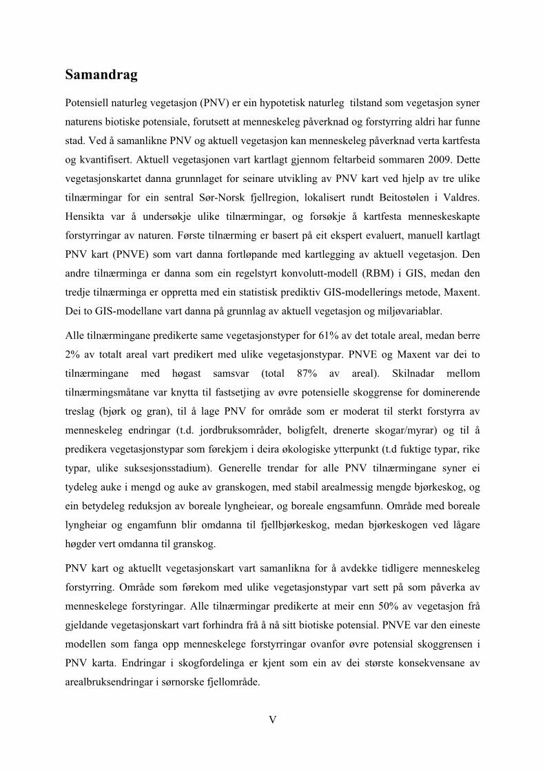
Table 1: Altitudinal vegetation type transition rules for the rule-based envelope modelling. See Appendix 2 for vegetation type description and Appendix 3 for additional information relating to the vegetation types.
Vegetation group Actual vegetation type Altitude (m a.s.l.) Potential vegetation type Poor and dry vegetation types
2c%, 2e% 2c%B 2c> 4a, 4a%] 7a&
< 1100 < 1100 < 1100 < 1000 < 1000
4a]% 4a]%B 4a]B 7a, 7a%] 7a
Intermediate vegetation types
2e, 2e!,2e& 2eg, 2eF, 2ej 2e!F 2e&< 2ev% 1b, 1bB,4b,7b& 4b]
< 1120 < 1100 < 1120 < 1120 < 1020 < 1020
4b 8c& 4b< 4b]% 7b 7b]
Rich vegetation types 3bs, 3b&s, 3bsg 3b,4c 4c, 4c] 7c&
< 1140 < 1140 1040 < 1040 < 1040
4c! 4c 7c, 7c] 7c
Wetlands and peatland forest
8c&, 8d& 9cs, 9c! 9cs, 9c!, 9c&! 9c& 9c& 9c&!k
< 1000 < 1050 950 < 950 < 1050 950 < 950 < 1050 950
8c*&, 8d*& 8c&! 8c*! 8d& 8d*& 8d&!
Anthropogenic types 11a 4g, 11b, 12d, 12e, 12f 4g, 11b, 12d, 12e, 12f 12f
< 1140 < 1120 1020 < 1020 > 1120
4c 4b 7b 2e
Ditched types 3bgT 4cT 9aT, 9cT 11aT, 8d&T 11bT, 12dT, 12eT, 12fT 11bT, 12dT, 12eT, 12fT
< 1100 < 1000
< 1000 < 1100 1000 < 1000
8d& 8d* 9a, 9c 8d*& 8c& 8c*
Unchanged types 1a 1b 2a, 2b 2c, 2e%, 2e., 2e:, 2eÅ 3a, 3b, 3b{ 7a, 7b, 7c 8c& 9a, 9b, 9c, 9e 12b, 12c
> 1120
> 1100 > 1140
> 1100
1a 1b 2a, 2b 2c, 2e%, 2e., 2e:, 2eÅ 3a, 3b{ 7a, 7b, 7c 8c& 9a, 9b, 9c, 9e 12b, 12c
2.3.2.1 Defining upper potential forest limit
Since modelling rules had to be manually set for the rule-based model, the upper potential
forest limit for birch and spruce needed to be manually identified. A forest is defined as an
area consisting of trees > 2.5 m high with a crown cover of at least 25% (Rekdal & Larsson
2005). The upper potential forest limits were identified in five ways (Table 2). First, the upper
potential forest limit was derived from the actual vegetation map and observations made
during the fieldwork. Second, the upper potential forest limit was identified from the PNVE

11
model. Third, the upper potential forest limit for birch was identified on a regional scale by
following the upper forest limit on eight surrounding topographic maps at a scale 1:50,000
(Norwegian Mapping Authorities N50 series, map number: 1616 I, 1616 IV, 1617 I, 1617 III,
1617 IV, 1716 IV, 1717 III, 1717 IV). The same method was also used for spruce, but was
done by following the upper forest limit on The Norwegian Forest and Landsca
area resource map (theme: type of wood) (TNFLI 2010) within the same area as for the
topographic maps (where the theme cover corresponded). Fourth, the upper potential forest
limit was found in registrations from a major subject survey carried out in the mid-1970s in
Øystre Slidre Municipality (Axelsen 1975). Fifth, and finally, the upper potential forest limit
(2000) registrations around Beitostølen from the early
1960s.
Table 2: Registration of upper forest limit and upper potential forest limit within and around the study area; p = poor forest, i = intermediate forest, r = rich forest.
Source Betula pubescens (m a.s.l.) Picea abies (m a.s.l.)
Vegetation map 990p/1100i/1070r 930p/850i/830r
Topographic map 1180 1080
Axelsen 1975 1130 1040*
Aas & Faarlund 2000 1100 975
Chosen upper potential forest limit 1140r/1120i/1100p 1040r/1020i/1000p *Registration from Mellsenstølane dairy farm cluster located c. 26 km south-east of Beitostølen.
2.3.3 Statistical predictive modelling
Maxent version 3.3.1, based on a maximum entropy algorithm (Phillips et al. 2006; Phillips &
Dudik 2008), was used to prepare a statistical predictive model for the potential distribution of
birch and spruce. Since Maxent uses occurrence data to develop the model, random plots were
assigned to vegetation types where birch and spruce occurred, either as primary or secondary
type of wood, using the Hawts analysis tools v.3.27 extension in ArcMap 9.3: 105 plots for
birch and 75 plots for spruce. A few plots (< 10) were added for both species to ensure good
spatial representation of both populations (Hengl et al. 2009). Since the vegetation figures
with spruce were distributed to a lower part of the study area, 27 additional plots were
assigned from single spruce stands identified from aerial photos to prevent bias in the
sampling and to provide a better basis for the later statistical modelling (Figure 2). High
resolution aerial photographs made it easy to identify separate spruce stands in the mountain
birch forest (Figure 3). Random spruce plots tended to serve as supplementary species-
presence data. Default values for all parameters (features, auto; regularization value, 1;
convergence threshold, 10 5; maximum iterations, 500; and background points, 10,000) were

12
accepted when running the model (Gibson et al. 2007; Riordan & Rundel 2009), except for
random test percentages, which were set at 25% for spruce and 30% for birch.
Figure 3: Aerial photo of spruce stands (a) and single spruces (b) in the mountain birch forest. (Scale 1:1500. (Source: www.norgeibilder.no, photographed June 2008)
The predictions results from Maxent are evaluated by a threshold-independent receiver
operating characteristic (ROC) analysis, known as AUC values, calculated within the
ict the relative distribution
probability of species (Elith et al. 2006). The closer to 1 these AUC values are, the greater the
e in a random prediction
model (i.e. no different from random models); values < 0.7 indicate poor prediction ability,
values 0.7 0.9 indicate moderate prediction ability; and values > 0.9 indicate significant
prediction performance (Pearce & Ferrier 2000).
cells with equal or lower value (Deblauwe et al. 2008; Phillips et al. 2006). The probability
scales are all relative occurrence probabilities, and therefore a given value is not directly
comparable to a value that is twice as high (Jimenez-Valverde & Lobo 2007). Sensible
threshold probability needs to be set when converting a continuous relative model to a
categorical map (Fielding & Bell 1997). Maximum sum threshold (MST) were used to set the
thresholds for upper potential forest limit in the Maxent predictions of spruce and birch
(Jimenez-Valverde & Lobo 2007). This is the value along the ROC curve which occurs at
greatest distance from the y = x line:
MST = Sensitivity (1-Training omission) + (1-Specificity(Fractional area))

13
Soil properties from the actual vegetation map were combined with Maxent distribution
predictions for birch and spruce in ArcMap to divide the predicted forest distribution into
poor, intermediate, rich, and peatland forest. For types 12d, 12e and 12f on actual vegetation
map, soil properties were derived and implemented from PNVE.
2.4 Uncertainty relating to the models
Making prediction models is difficult and there are many uncertainties (Barry & Elith 2006).
Two different uncertainty maps were designed to assess uncertainties between the different
models and in the modelling of various vegetation types. An overlay procedure was run
between the three prediction models to assess the differences among the prediction models.
The predictions were compared on vegetation type level (without additional information). The
uncertainty map for modelling vegetation types was based on expert knowledge of how
different ecological characteristics can affect the development towards a natural dynamic
equilibrium state.
2.5 Anthropogenic influence
The actual vegetation map was compared thr
ArcMap 9.3 (Ormsby et al. 2001) with PNV maps, to identify anthropogenic influences on the
nature and vegetation structure in the study area. The differences between the vegetation types
on the actual vegetation map and the PNV maps were considered to be due to anthropogenic
influences (Bryn 2009; Gehrig-Fasel et al. 2007), since these types have not yet reached their
natural state of dynamic equilibrium (Bryn 2009).
2.5.1 Vegetation transitions
The vegetation group changes were derived from the area information relating to each PNV-
map and exported for calculation and comparison in Microsoft Excel 2007. The comparisons
of the upper potential forest limits were performed using a grid resolution of 100 m. The
upper forest limit for each vegetation map was derived in the crossover to the grid. To assess
the quantity of each vegetation type that was transformed to other vegetation type(s), a point
grid with 50 m spacing was used, resulting in 13,695 representative points (Nakagoshi et al.
1998). Information about actual vegetation and PNVE vegetation was assigned to the points.
Points with vegetation information were used to calculate the vegetation transitions among
models.

14
2.6 Statistics
Statistical tests were performed using SPSS (Statistical Package for Social Science) Version
17. Differences between the models in mean altitudinal changes of potential upper forest limit
were tested with the Kruskal-Wallis one-way analysis of variance with subsequent Mann-
Whitney U-tests. Divergence in the previous average summer temperature (1962-1986) from
the recent average summer temperature (1997-2009) were tested with the Mann-Withney U-
test. Non-parametric tests were used in both cases. The cause for this was non-normal data
distribution and different variability in the data-sets (Mackenzie 2005).
3 Results
3.1 Model accordance
The three PNV-models predicted the same vegetation types for 61% of the study area (Table
3; Figure 4). Only 2% of the area differed among all three PNV models. Common to the
vegetation types within the 2% is that they are influenced by different soil moisture levels.
They grow in bog, peatland forest, drained agricultural land, or ditched non-productive areas,
or where alpine heath and/or meadow communities occurring between different modelled
potential forest limits. Only PNVE and RBM models predict the same vegetation type for
10% of total area (71% in total), which is mainly where the Maxent model predicts lower
upper potential forest limits for both birch and spruce. Only the Maxent model and PNVE
predicted same vegetation types for 26% of total area (87% in total), which is mainly between
the upper potential forest limit for spruce and birch.
Table 3: Area calculations of model accordance among the different models.
Accordance among: Area (km2) % of total area All models 21 61% No models 0,6 2% RBM and Maxent 0,4 1% PNVE and Maxent 8,8 26% PNVE and RBM 3,3 10% Total 34,2 100%

15
Figure 4: Accordance map of comparisons between the outputs of the different PNV models. Map projection WGS84/UTM zone 33N.
In general, there is greater uncertainty related to the modelling of PNV at higher altitudes in
alpine heath or alpine meadow communities (Figure 5). Below the potential forest limit, the
greatest modelling uncertainty relates to non-productive areas (12c, 12d, 12f), farmland (11a,
11b), and other areas which are largely under anthropogenic influences (e.g. drained forests).
The greatest certainty for modelling at lower altitudes relates to wetlands and spruce forests.
The large share of birch forest in the study area is modelled with comparatively less
uncertainty.

16
Figure 5: Map of uncertainty for modelling different vegetation types. Map projection WGS84/UTM zone 33N.

17
3.2 Anthropogenic influence
The divergence between the actual vegetation map of 2009 and the three PNV maps is
probably a result of long and frequent human disturbances (see Discussion), and hereafter
affected areas are referred to as anthropogenically influenced areas. All three PNV models
estimated that more than 50% of vegetation recorded on the actual vegetation map still has not
reached its expected natural dynamic equilibrium status (Figure 6; Table 4).
Figure 6: Variation between the models on predicted human influence within the study area. Map projection WGS84/UTM zone 33N.

18
The RBM predicted the highest difference from the actual vegetation map (60%) (Table 4),
while the Maxent model predicted the lowest difference from the actual vegetation map (54%)
(Table 4). The area with the greatest influenced is situated below the upper potential forest
limit. The small shares of influenced areas situated above the potential forest limit are small
units of pasture or non-productive areas on the actual vegetation map (Figure 7). The PNVE
model is the only method which predicts human disturbance above the upper potential forest
limit for vegetation types other than the 12 types. Further, it was found that anthropogenic
influences had mainly disturbed the development of lichen heaths.
Table 4: Predicted anthropogenic influences among different PNV models.
Model Anthropogenicaly influenced area (km2)
% of total area
PNVE 19.2 56% RBM 20.6 60% Maxent 18.5 54%

19
3.3 Vegetation type change
The actual vegetation situation (Figure 7) differs considerably from all three PNV maps
(Figures 8 10). More than 50% of the area changes vegetation type on PNV maps. General
tendencies for all of the PNV models show increasing amounts of spruce forest, with
subsequent decreasing amounts of alpine heath and alpine meadow communities, and with a
stable proportion of birch forest (Figures 8 10). Areas with alpine heath and alpine meadow
communities are transformed into mountain birch forest, whereas birch forest at lower
altitudes is transformed into spruce forest. In addition, all pastures, cultivated land, and
human-made, non-productive areas were excluded from the PNV models.
Figure 7: Vegetation map from the area around Beitostølen in 2009. Map projection WGS84/UTM zone 33N.

20
The landscape changes from the actual vegetation map to PNVE were dominated by the
expansion of spruce forest and reduction in alpine vegetation types, particularly alpine heath
communities (Figure 8). The expansion of spruce added 10.6km2 to the total spruce forest in
the area. Almost 80% of the actual birch forest has been transformed into spruce forest.
Despite this, the amount of birch forest is roughly stable (aberration 0.1 km2 compared to the
actual vegetation map).
Figure 8: Vegetation map produced using the expert-evaluated PNV model (PNVE). Map projection WGS84/UTM zone 33N.
21
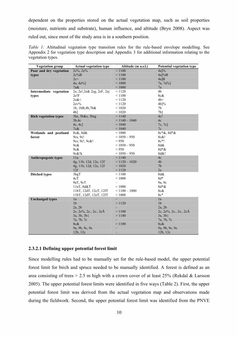
The landscapes changes from the actual vegetation map to the RBM were dominated by
reductions in the alpine heath and meadow communities and birch forest, while the spruce
forest advanced (Figure 9). Both spruce and birch forest advanced to higher altitudes, but
there was a corresponding decrease in birch forest as spruce forest expanded. This PNV
models predicts the highest amount of spruce forest (15.7 km2) and the largest advance for
peatland forests (1.4 km2) at the expense of wetlands.
Figure 9: Vegetation map produced using the rule-based envelope PNV model (RBM). Map projection WGS84/UTM zone 33N.

22
The landscapes changes from the actual vegetation map to the Maxent model were dominated
by a small reduction in alpine heath communities and the advance of spruce forest (Figure
10). This method models the lowest reduction in alpine vegetation types, and the smallest
expansion of the spruce forest (9.1 km2 in total). The total area with birch forest is almost
equal to that on the actual vegetation map (8.3 km2), but is displaced to higher altitudes.
Figure 10: Vegetation map produced using the Maxent-predicted PNV model. Map projection WGS84/UTM zone 33N.
The elevation advance of birch and spruce forest to higher altitudes would reduce the alpine
vegetation from 12.3 km2 to 5.8 km2 in the PNVE model, 5.1 km2 in the RBM, and 7.8 km2 in
the Maxent model. Snow-bed vegetation would not be affected, but approximately half of the
area of alpine heath communities and meadow communities would be replaced, and the
majority of birch forest (Figure 12). In addition, a small share at lower altitudes would be
replaced with spruce forest. All models predict that spruce will expand in terms of both
altitude and land cover. On the actual vegetation map covers spruce forest only 2.4% of the
total area. All models predict a considerable increase, to 30.9% in the PNVE, 46.2% in the
RBM, and 26.7% in the Maxent model. The total area of birch forest is predicted to be stable
according to the actual vegetation map in the PNVE model and the Maxent model, while in
the RBM birch forest covers a considerably lower area (Figure 11).

23
Figure 11: Vegetation groups as a percentage of total area (34.2 km2). Total area statistic for vegetation types in Appendix 2.
The vegetation group expected to show the largest advance is spruce forest. Almost every
vegetation group has the potential for spruce forest, with the exception of snow-bed
vegetation, peatland forest, wetlands, and natural non-productive areas. All models predict
that peatland forest has a slightly larger potential than observed in the actual vegetation. The
potential is located in the alpine meadow communities, non-productive areas, and wetlands.
Despite this increased potential, a small share of the peatland forest has the potential for being
wetlands (Figure 12). The proportion of wetland seems stable and undisturbed (Figure 11),
but the low share (3.5%) that is transferred to peatland forest is replaced with very low
proportions of non-productive areas, farmland, and alpine meadow communities. Among the
alpine vegetation, alpine heath communities are expected to experience the largest reduction
in total area. However, in the PNVE model, alpine meadow communities are predicted to
experience the largest reduction in percentage (c.78%) of their original area. The majority of
alpine meadow communities will be transferred to birch forest on firm ground. The small
areas of humid types will be transferred to wetlands and peatland forest. The majority of the
farmland on the actual vegetation map (73%) originally have the potential for being spruce
forest, while smaller shares have the potential for birch forest (17.7%), wetlands (7.7%), and a
negligible proportion of alpine meadow communities (Figure 12).
0%
10%
20%
30%
40%
50%
60%
70%
80%
90%
100%
Actual PNVE RBM Maxent
Vegetation map
1 Snow-bed vegetation
2 Alpine heath communities
3 Alpine meadowcommunities
4 Deciduous forest
7 Spruce forest
8 Peatland forest
9 Wetlands
11 Farmland
12 Non-productive areas

24
Figure 12: Main vegetation transition from present situation to expert-evaluated PNV model. The area given in square kilometres is the area in the present situation. The percentages refer to the proportion of the present vegetation group transferred to a given vegetation type.
3.3.1 Maxent prediction
The Maxent predictions for the distribution of spruce forest (AUC = 0.883)(Appendix 4) were
better than predictions for birch forest (AUC = 0.769)(Appendix 5). According to the built-in
jackknife procedure in Maxent, the proxy variable for temperature (DEM) contributed most to
the potential spruce forest model (73%), while soil properties contributed considerably to the
development of the potential birch forest model (56%). Calculation of MST resulted in
choosing cumulative value 13 for spruce and 4 for birch when drawing maximum dispersal of
the species.
3.4 Forest limit change
The RBM predicts the highest altitudinal average forest limit for both birch (1116 m a.s.l.)
and spruce (1026 m a.s.l.), while the Maxent model predicts the lowest altitudinal average
forest limit for both birch (1055 m a.s.l.) and spruce (950 m a.s.l.) (Figure 13).

25
Figure 13: Average altitude for the present situation and the three vegetation models based on the grid dataset (Error bars: 95% CI).
The present mean continuous upper potential forest limit for birch and spruce is significantly
reduced (p < 0.001) according to all three PNV models. The general situation shows that the
quantity of birch forest recorded on the actual vegetation map will remain stable (Figure 11)
on the PNV maps, but will become displaced to higher altitudes. The actual vegetation map
shows that 25.5% of the area is covered with birch forest. This is almost equal to the PNVE
and Maxent predictions, which respectively predict that 25.5% and 24.1% of the total area has
the potential for birch forest at the theoretical dynamic equilibrium state (Figure 11). This is
not the situation for the RBM, which predicted the elevation for spruce to be considerable
higher and on this basis predicts the distribution of mountain birch to be less extensive, i.e.
only 12.7% of total area.
The statistical test of difference in average summer temperature (June, July and August)
showed a significant change (p<0.05) on 1 °C from recent temperature registrations (1997-
2009), 12.7 °C, compared to older temperature registrations (1962-1986), 11.7 °C.

26
4 Discussion
4.1 Modelling methods
Vegetation maps have proved to be useful in spatial GIS-modelling (Bryn 2008; Carranza et
al. 2003; Chytry 1998; Dirnbock et al. 2003; Moravec 1998; Tichy 1999). In the present study
three different modelling methods were used, resulting in three different PNV maps. The three
maps made predictions with a fault rate of < 40% according to corresponding vegetation
types. In general, the different models result in similar trends on the PNV maps.
First, the three models predict different altitudinal levels for the upper potential forest limit.
The RBM predicts the highest altitudinal forest limit with minimal vertical variation. This is
not affected by ecological properties or altitudinal variations that may occur on a small spatial
scale. Instead, is it related to the concepts of exploratory modelling, as well as envelope
modelling. The goal of exploratory modelling is to capture key traits and general trends, and
the details are less important (Perry & Millington 2008), whereas the methodology of
envelope modelling restricts variations within the chosen envelope (Guisan & Zimmermann
2000). PNVE and Maxent are contrasting modelling methods to RBM, and make allowances
for ecological differences and gradients to a larger degree than RBM.
Second, all modelling methods have problems with modelling PNV on types strongly
influenced by human disturbance (i.e. types 11a, 11b, 12d, 12e, and 12f). Especially drained
types from vegetation groups 11 and 12 are modelled differently among all models. Human-
modified areas where the original vegetation has been completely removed and where
restoration is impossible are hard to model. It was originally recommended that these types
should be excluded from the modelling and left as open areas on the PNV map (Tüxen 1956).
More recently, Moravec (1998) and Zerbe (1998) have recommended that these types should
be manually interpreted on the PNV map to reduce uncertainty. This uncertainty is especially
present in the RBM and Maxent models. Uncertainty in modelling these types is almost
avoided on the PNVE map since this map is based on field observations and created by using
the remaining fragments of intact vegetation as a reference point (Moravec 1998). The PNVE
is the only model which gives good predictions for vegetation types 12c, 12d and 12e.
Third, modelling performs well on successional vegetation types, but is complicated where
types occur in their ecological extremities. Especially factors such as humidity, nutrient
richness, and successional state complicate the modelling. The fact that the PNVE model
captures extremities for types is related to the PNVE model being compiled from actual
vegetation in the field. Observations of species composition and physiognomy in field may

27
explain why some types are predicted to develop differently than when modelled with RBM
and Maxent, and why variations in additional information that were meant to capture
ecological extremities did not work as well in models as anticipated. For example, semi-
humid types may appear in a state that is not humid enough to be identified using the
additional sign of humidity. This may also be the case with the poorer types, e.g. poor types of
dwarf shrub heath are modelled to lichen and heather birch forest in PNVE, while Maxent and
RBM model the same polygons to blueberry birch forest. This may be due either to
insufficient registration of additional information regarding poor/shallow soil, or insufficient
implementation of rules in the RBM. The assumption during the vegetation mapping was that
poor types were intercepted with additional information regarding bare ground, soil depth or
lichen cover. Disturbance in lichen cover is an additional information sign that probably
should be included in future surveys. PNVE was the only model that captured disturbance
above the present forest limit in alpine heath communities. Disturbance was especially related
to lichen cover in lichen heaths. Here, it is evident that additional information did not capture
all essential information for later GIS-modelling of vegetation disturbance.
4.1.1 What is modelled?
From a literature search, the modelling from this study does not appear to fall into any
specific classification, except for the general acknowledge that it models the potential
distribution of species. Products from distribution models based on species data and
(Capelo et al. 2007),
(Soberon & Peterson 2005) (Li et al.
2009; Peterson et al. 2007), among other terms. Hence, it is the inconsistent use of terms and
different understandings of the niche concept in species distribution modelling/models (SDM)
which contributes to the uncertainty of what prediction outputs represents (Kearney 2006).
There are at least three main niche theories implemented in the various SDMs: i) Grinellian
niche, environmental characteristics needed by a species to survive in without immigration
(Grinnell 1917); ii) Eltonian niche, species interactions with other species (Elton 1927); and
-dimensional hypervolume, where species are not able to utilize their entire
fundamental niche, but are limited to their realized niche due to biological interactions,
mainly focused on competition (Hutchinson 1957). However, each of these concepts has been
modified and criticized since they have been introduced (Hirzel & Le Lay 2008). Theories
that have developed in recent decades, e.g. the metapopulation theory (see e.g. (Hanski 1999))
and the source-sink theory (see e.g. (Pulliam 1988)), have shown the limitations of these niche
definitions.

28
The rule-
- (Guisan & Zimmermann 2000; Heikkinen et al. 2006). The
statistical Maxent modelling technique used in this study is also an SDM (Phillips et al. 2006;
Phillips & Dudik 2008). According to Phillips et al. (2006) is also Maxent a niche-based
model where the output represents the modelled species niche in relation to the actual
species distributions using the relationships between species occurrence data and
environmental predictor variables as the basis (Raes & ter Steege 2007). According to Guisan
& Thuiller (2005), the output of SDMs is a map of habitat suitability. Habitat suitability
models (HSM) assume that a species-
environmental
However, HSMs make good contributions in revealing the niche characteristics of species
(Hirzel & Le Lay 2008). Kearney (2006 p. 190)
the association between organisms and featu
the vegetation classes used in this study. In other words, modelling of the vegetation maps
might be considered a type of habitat modelling. However, it cannot be implemented in the
HSM term since it models habitat distribution rather than possible habitats for species. The
special advantage with the Maxent model in this study is that the predicted distribution for
birch and spruce (species) forms the foundation for the potential spatial distribution of the
vegetation types (habitats) associated with these species.
The modelling performed in this study did not include sufficiently complex environmental
variables which may contribute to the modelling of species niches. However, the possible
distribution of species is modelled on a spatial scale based on environmental variables. A
better term for the Maxent modelling would therefore probably be spatial prediction
modelling (SPM), a term coined by Rune Halvorsen (30. April 2010 at the University of
Oslo).
4.1.2 Environmental variables
The GIS-based models are designed to be produced with minimal complexity with vegetation
types were changes and succession patterns are known from an earlier study (Bryn 2008),
where time series were used to identify a similar but more restricted modelling. In general, the
selection of environmental variables is crucial and often relies on expert knowledge (Guisan
& Zimmermann 2000; Manel et al. 2001). However, the purpose of modelling and scientific

29
experience was normative for the variables selected for the modelling (Metzger et al. 2005),
together with the available variables (Bakkestuen et al. 2008). The DEM and the soil
characteristics were the only two available predictors in proper resolution for our study area
which contributed in the modelling of the PNV maps.
4.1.3 Time aspect
A high level of uncertainty is associated with determining the time aspect for the occurrence
of the predicted changes to the PNV maps, or whether it will occur at all. A variety of biotic
and abiotic factors may affect the successional regrowth rate and forest establishment, and
hence the same vegetation type may transform at different rates at different locations due to
different microclimatic conditions and historical use (Huntley 2005). This idiosyncratic
in birch
establishes relatively fast, while spruce establishes more slowly. Hence, the history of
anthropogenic disturbances and landscape properties affect the vegetation dynamics and
regrowth patterns (Didier 2001). Regrowth does not react as a linear response to land
abandonment (Bryn 2006). Therefore may areas that apparently seem to be in different
successional stages have been abandoned at the same time. It is also difficult to assess when
abandonment terminated, but increased time since abandonment favours succession and
natural regrowth (Tasser et al. 2007). In addition to optimal climate conditions (Dalen &
Hofgaard 2005), do successional regrowth speed depends on factors such as geology,
elevation, exposure, and slope. After land abandonment do, especially elevation, soil moisture
and nutrient status play an important role in successional regrowth speed (Bryn et al. In press;
Tasser & Tappeiner 2002). Numerous factors might have influenced the vegetation
disturbances around Beitostølen. Earlier, grazing, forage harvesting, logging, and other
agricultural related activities dominated the use of outfields in the study area (Gjesdahl 1965).
Decreased grazing in the outfields and the reduced need for firewood are the main controlling
factors for forest regeneration after abandonment of summer dairy farms in the Swiss Alps
(Gehrig-Fasel et al. 2007; Gellrich & Zimmermann 2007). Grazing by domestic animals
especially affects birch forest where logging and mowing is also practised (Bryn & Daugstad
2001). Decline in these activities presumably can explain the established anthropogenic
influence within the study area.
The recent increase in summer temperature within the study area (figure 2), have probably
contributed to increased forest growth and elevated potential forest limits (Barnett et al. 2001;
Bjune 2005). However, this would not have changed the PNV models of this study. Firstly,
the recent climate improvement are not yet reflected in higher actual forest limits. Kullmann

30
(2001) proposed a time-lag of 30 years in Sweden for the forest limit to respond to changing
climate. If the summer temperature continue to increase, the upper potential forest limit will
be raised to higher elevations than expected in this study, because the upper potential forest
limit is correlated with summer temperature (Bryn 2008; Mäkinen et al. 2002). If this is the
case, the PNV models presented in this study will underestimate the potential forest regrowth,
but at the same time you will be sure not to exagerate the effect of human disturbance.
Secondly, improved temperatures can increase the regrowth rate and subsequently speed up
the succession towards the PNV condition (Rössler et al. 2008). Thirdly, increased summer
temperature would drive the forest to higher elevations (Moen et al. 2004). However, this
study models PNV related to the present environmental conditions. Raised summer
temperatures would change the conditions and subsequently give other PNV models.
4.1.4 Reliability
The PNV maps are hypothetic models of a natural ecosystem, which probably will never be
reached. The main purpose of preparing such maps is to gain an overview of which areas are
influenced by humans and what these influenced areas will transform into when human use
cease. These maps show the relationship between vegetation types and environmental
variables, and will provide a good basis for decision making in management issues (Gallizia
Vuerich et al. 2001). Besides being a good starting point in management issues, the PNV
maps are a good null model for modelling climatic scenarios (Bryn 2009; Lapola et al. 2008;
Rio & Penas 2006). Producing climatic scenarios without taking anthropogenic disturbances
into consideration will give incorrect results and furthermore the estimates of vegetation
response to climatic changes will be incorrect too. There is great difficulty in modelling
climatic changes in relation to non-ecological factors (Rössler & Löffler 2007). This applies
especially to the development of the forest limit (Hofgaard 1997; Holtmeier 2003). As a
consequence, models which assume a direct relationship between the present forest limit and
the climate will make incorrect predictions on a regional scale (Rössler & Löffler 2007).
4.1.5 Objectivity
It is difficult to model PNV without including a degree of subjective judgment (Capelo et al.
2007). PNVE is model with highest subjectivity since it is created with expert knowledge as
the basis. The RBM is objective and based on ecological findings, but also has elements of
subjectivity since some rules are implemented with a basis in knowledge and not based on
findings from the study area. The Maxent model performs with the greatest objectivity since it
is based on ecological findings which work as a foundation for statistical modelling. Even

31
though the RBM and Maxent are considered more objective methods for mapping compared
to PNVE, they may also have been affected by subjectivity during the mapping of actual
vegetation. The subjective decisions are related to the drawing of borders between different
vegetation types during fieldwork (Tichy 1999). Also, Maxent will not perform very well in
areas that have high levels of human disturbance. Maxent relies totally on the present
distribution pattern of modelled species and might therefore underestimate the potential
distribution of species that are highly influenced by the human disturbance. In contrast, RMB
is more appropriate for modelling types or species which are suppressed by anthropogenic
disturbance. Hence, objectivity is maintained by using findings from the study area which are
adjusted based on ecological knowledge.
4.1.6 Scale
The PNV models discussed in this study present potential vegetation transitions on vegetation
type level, representing the scale of the classification system used for field registrations. The
use of another system, e.g. Naturtyper i Norge (Nature types in Norway) (NiN) (Halvorsen et
al. 2008) or a more detailed vegetation mapping system, e.g. Fremstad (1997), would provide
vegetation classification at a smaller scale. Identification of vegetation and vegetation
transitions at smaller scale leads to more variation in the vegetation pattern, and hence predict
greater amounts of human-influenced land. In contrast, vegetation classification on a larger
scale would predict both less variation in vegetation and less anthropogenic influence.
4.1.7 Manual made expert-evaluated potential natural vegetation map
PNV map based on field registrations must be assumed to be the most precise and credible
model, since they are based purely on field observations of remaining actual vegetation.
According to Tüxens (1956) original proposal for creating PNV maps, this is one of the
strengths with this method. The field-related method provides larger larger possibilities for
capturing vegetation gradients, which occurs in ecological extremities, successions, or small-
scale variation. This variations might be generalized and neglected in the actual vegetation
maps, which are the basis for modelling PNV with RBM and Maxent. Thus, this method
provides a better method in reconstructing areas exposed to heavily human alterations, since
small patches of vegetation still may provide information of e.g. physiognomy, soil type and
humidity, which contributes to reveal earlier vegetation types. However, heavily human
disturbed areas are often proposed to be left outside in models of PNV (Moravec 1998).

32
4.1.8 Rule-based model
The RBM model is the most general model and captures the key traits rather than the small-
scale changes (Perry & Millington 2008). The purpose of envelope modelling is described by
Malczewski (2000 p. 21)
GIS-based decision analysis is to provide insights and understanding, rather than to prescribe
model captures the key traits, it was nevertheless
developed to be as correct as possible (like PNVE). The greatest uncertainty related to this
model, apart from modelling the heavily human-utilized areas, is probably connected with
drawing the upper border of potential forest limit. However, PNV modelling at a larger scale
than 1:25,000 reduces the problems connected with drawing exact borders (Bryn 2008;
Chytry 1998; Ricotta et al. 2002).
detecting complex ecological systems (Perry & Millington 2008). Accordingly, are this
strategy used for exploring human disturbance and testing the effects of different management
strategies (Bryn 2006; Perry & Millington 2008).
4.1.9 Maxent
The use of presence-only data has proved useful for modelling species distribution (Elith et al.
2006; Riordan & Rundel 2009; Wollan et al. 2008). Maxent is among the GIS-modelling
techniques that give the best predictions (Elith et al. 2006). In addition, it has the capability to
make appropriate distribution predictions beyond the present realized distribution (Phillips et
al. 2006). Even though models based on presence-only data are regarded as being less precise
than presence/absence models, presence-only and presence/absence models are closely
correlated (Hirzel et al. 2006).
Evaluation and defining threshold
Statistical Maxent models for birch and spruce performed better than moderately well (AUC
< 0.7). This means that both predictions performed well, but not perfectly. However, AUC
values tend to be higher for species with narrower ecological amplitude, without the model
necessarily being better (Phillips & Dudik 2008). Since both birch and spruce are more
generalists then specialists, both models can be more precise than evaluation through AUC
values. This can indicate that the predicted distribution of both tree species is good overall.
The evaluation by predictive distribution models with a threshold-independent accuracy
measure, such as ROC (AUC-values), is standard procedure for the evaluation of biological
prediction models (Fielding & Bell 1997), but has received criticism in recent years (Austin

33
2007; Lobo et al. 2008). AUC is the only measure that can translate continuous prediction
models as present/absence sites without threshold definition (Zucchetta et al. In press).
Evaluation through AUC relates true positive predictions and false positive predictions to
results in a continuous range of threshold levels (Cumming 2000; Erasmus et al. 2002).
(Liu et al. 2005). Continuous
probabilities prediction from species distribution models needs to define a specific threshold
for converting the predictions to presence/absence on a map. There are several ways of
defining thresholds for conversion of continuous maps to categorical presence/absence maps
(Jimenez-Valverde & Lobo 2007; Liu et al. 2005). In the present study threshold was derived
from the values in a ROC plot, although ROC plots in themselves do not provide such
classification rules (Fielding & Bell 1997). Jimenez-Valverde & Lobo (2007) found that
defining thresholds based on the relationship between the ROC-plots sensitivity and
specificity values (minimized different threshold (MDT) and MST) produced the most
accurate predictions. Hence, these were most related to prevalence of the test species. MDT
balances the relationship between sensitivity and specificity (Cantor et al. 1999), while MST
(Manel et al. 2001). MST was used in this study since it was
more important for identifying the distribution of birch and spruce than identifying their
absence.
Samples
There is no given rule on how many sample points are needed to form the basis for a
satisfactory prediction. The number depends to a large extent on the properties of the study
area and the selected species. In general, smaller sample sizes lead to lower levels of accuracy
(Hernandez et al. 2006). However, accuracy is usually greater for species with more
specialized niches (Chahouki et al. 2010; Hernandez et al. 2006; Phillips et al. 2006). Since
birch and spruce can be classified as more general species (Lid et al. 2005), this may have
affected the modelling performance by leading to lower AUC values (Phillips & Dudik 2008).
However, Hengl et al. (2009) emphasize that the geographical representation of samples is
much more important than the number of samples.
The statistical modelling of Maxent is one method for species distribution modelling (SDM).
The purpose of SDM is to spatially predict species occurrence using the relationships between
species occurrence data and environmental predictors as the basis (Raes & ter Steege 2007).
The special advantage of this method is that the prediction models for birch and spruce form
the foundation for the potential distribution of vegetation types (habitat).
34
Species distribution models (SDMs) attempt to predict the potential distribution of species by
interpolating identified relationships between species presence/absence or presence-only data
on the one hand, and environmental predictors on the other hand, to a geographical area of
interest.
Maxent: Modelling of forest limit, treeline or species limit
Modelling based on species occurrence data, as mentioned above, results in a habitat
suitability model (HSM) for actual species. When modelling the potential distribution of tree
species, as was done in this study, the question arises as to whether the output map represents
the upper potential forest limit of the trees, the treeline, or the upper potential presence for the
actual species. For the present study, a tree is defined as a full-grown individual, standing 2.5
m tall in the case of birch and 5.0 m tall in the case of spruce. The treeline is the uppermost
border for normally formed trees above the upper potential forest limit, while the species limit
is the upper boundary at which the species occurs (Aas & Faarlund 2000).
The answer to the above question may be neither definite nor exact. The output from the
models represents the input for the predictions. Thus, if the occurrence data represent the
highest occurrences of trees within the area, the output will probably also represent the same.
On the other hand, if the modelling is performed with upper findings from established forest
of actual tree species, is it more likely that the prediction model will reflect the upper potential
forest limit for that tree species within the actual area. Another aspect in this consideration is
how the threshold for drawing the exact distribution border from the relative prediction scale
is defined. Clearly, different threshold definitions result in a different predicted result
(Jimenez-Valverde & Lobo 2007).
4. 2 Vegetation transitions and anthropogenic disturbance
The actual vegetation map (AVM) and PNV maps show differences for most of the
investigated area. This indicates that a large share of the present vegetation still has not
reached its natural state of dynamic equilibrium (Ricotta et al. 2000) and is prevented from
reaching this state due to continued human disturbance and the time lag needed for forest
establishment at these altitudes. Hence, the development of the disturbed areas is assumed to
be prevented by anthropogenic influences (Ricotta et al. 2000), since the development of
natural succession is known to be disturbed by such influences (Gellrich et al. 2007;
MacDonald et al. 2000; Olsson et al. 2000).

35
Termination or strongly reduced management immediately initiates a state of natural
succession (regrowth) (Fremstad & Moen 2001; Potthoff 2007; Tasser & Tappeiner 2002).
Natural regrowth is an ongoing trend observed in all Norwegian mountain regions (Aas &
Faarlund 1995; Bryn 2008; Bryn & Debella-Gilo 2010 In Press). The same trend is also
observed in the Swiss Alps, where it has been observed as regrowth following agricultural
abandonment (Gehrig-Fasel et al. 2007; Gellrich et al. 2008; Motta & Nola 2001). The
influenced area around Beitostølen is primarily situated below the existing forest limit. This
largely corresponds to most of the forested landscapes being influenced by humans (Bryn
2009; Garbarino et al. 2009). Large areas below the present upper potential forest limit are
disturbed in the natural development towards the dynamic equilibrium state by human
activities. Logging, grazing and mowing are among the historical activities with the greatest
impact on this development. Hence, these activities decreased considerably in Norway after
1950s (Almås et al. 2004). Above the existing forest limit, alpine pastures, agricultural land,
and land with grass and scrub vegetation are all primarily influenced by human activities
(Gellrich et al. 2007). This trend has also been observed within the study area.
The identification of earlier anthropogenic disturbance and subsequent regrowth within the
study area indicates a trend of decreased human nature utilization, where human actions are
intensified and concentrated, with considerably greater ecological consequences. Modelling
and mapping using PNV models substantiates this finding where the heavily disturbed classes
(11a, 12c, 12d and 12e) were very difficult to model and map due to the fact that there were
few traces of actual vegetation. Vegetation types exposed to medium disturbance (11b,
drained forest, peatland forest and mires) were also mapped and modelled with high degrees
of uncertainty, but more traces of actual vegetation, makes the construction of PNV for these
types more reliable. This reflects the dominant trend for the development of the landscape in
Norway. Where the introduction of machines and fertilizer has led to increasing demands for
productivity and effectivity with subsequent intensification of the agricultural industry, the
mosaic-dominated landscape has gradually disappeared (Dramstad & Puschmann 2008).
Research from European mountain areas has revealed similar traces of reduced human
utilization of outfields but decreased intensification of utilized areas (Gellrich et al. 2007;
Gellrich & Zimmermann 2007; MacDonald et al. 2000). Gellrich & Zimmermann (2007)
proved that abandonment of agricultural areas in Swiss mountains first occurred in areas with
poor and shallow soil properties, where the slopes are steep or the road infrastructure is poor
developed. Abandonment took place where most of the employees primarily worked in
connection with the secondary and tertiary sectors. This corresponds well with the

36
employment situation in Øystre Slidre Municipality, where c.90% of workforce is related to
these two sectors (SSB 2009).
Bryn (In press 2010) showed statistically that the intensity of human land-use within the
outfields was higher closer to farms and summar dairy farms than further away. According to
Bryn, the consequence of more intensive land-use was higher probability of deforested areas
surrounding the farms and summar dairy farms. It is therefore likely that the findings reported
here, also mainly relates to human disturbance. Alternative explanations, e.g. forest fires or
caterpillar outbreaks, might have influenced the within vegetation type variation, but will
most probably not have shifted the vegetation types per se. The vegetation type transitions
modelled as the difference between PNV and AVM, is also spatially closely linked to the
farms and summar dairy farms.
Forest regeneration will occur up to the upper potential forest limit if the abandonment of
agricultural activities ceases, and natural succession will occur without interference (Gehrig-
Fasel et al. 2007; Gellrich et al. 2007). This represents a natural succession to a dynamic
equilibrium state dominated by coniferous forest. Clearings within coniferous forest initiate
the first succession step back to coniferous forest with a colonization and regrowth session of
birch (Aas & Faarlund 1996). Birch forest also constitutes a climax state between coniferous
forest and alpine vegetation in Scandinavian mountains (Aas & Faarlund 1995).
4.2.1 Unchanged types
Several vegetation types have not been modified, particularly fens, peatland forest, and snow-
bed vegetation. These types may either have been clear of former human land-use or the
length of time since such disturbance has been sufficient that they are now in a late natural
succession state (Bryn 2006). Formerly, scything and grazing on fens in Norway were
commonly practised to accumulate stores of fodder, but mainly ceased after World War II
(Almås et al. 2004). This was also a common practice on the fens in the study area (Gjesdahl
1965). Thus, it is probable that fen types in the area have been disturbed in the past and occur
today in a later natural succession state.
4.3 Forest limit changes
The PNV maps indicate that there is great potential for forest distribution to increase in the
investigated area, with elevated upper forest limits for birch and spruce. This reflects the
potential for forest expansion into the mountain region of southern Norway (Aas & Faarlund
1995; Bryn 2008). The forest expansion is probably related to altered and decreasing

37
agricultural activities in the outfields. Earlier, logging cleared the forests and subsequent
mowing and grazing in outfields prevented forests from establishing in mountain areas.
Studies from Norway (Bryn 2008) and mountainous countries in Europe (Capelo et al. 2007;
Carranza et al. 2003; Chahouki et al. 2010; Gehrig-Fasel et al. 2007; Wallentin et al. 2008)
indicate that the observed expansion of forest limits is related to regrowth after earlier land-
use and the abandonment of traditional agricultural management.
A northern and height-related expansion of the boreal forest has been observed since the
beginning of the 20th century (Vittoz et al. 2008). This has been explained as due to the
increasing temperatures after the Little Ice Age (Esper et al. 2002), since treeline vegetation in
Fennoscandia is sensitive to climate-related environmental changes (Seppä et al. 2002).
However, it is important to distinguish between the elevation of forest limits resulting from
climatic changes and those influenced by land abandonment (Bryn 2009; Tinner & Theurillat
2003). Several authors agree that the observed forest limit expansion is a response to changing
climate (Holtmeier & Broll 2005; Kullman 2001) since the upper potential forest line is
constrained by air temperature (Körner 1998). This may be supported by the fact that the
forest limit in Norway has fluctuated through time and forests have been established
considerably higher than seen today. For instance, pollen analysis (Bjune 2005) and analysis
of macrofossils (Aas & Faarlund 1988) have revealed that in the past birch forest has grown
up to c.1300 m a.s.l. in Mid-Holocene in Jotunheimen. However, it has been documented by
several researchers that most of the forest expansion that has appeared during the last 50 years
in mountainous Norway has been primarily driven by the lack of human disturbance (Bryn
2008; Engum 2006; Rössler et al. 2008). These authors also point to climatically improved
growth conditions in the last decade, and claim that this will probably speed up the future
regrowth rate and further raise the upper potential climatic forest limit. In the last 50 years,
however, the impact of climate changes on the regrowth rate and upper potential forest has
been very low compared to the effect of reduced land-use (Bryn 2009). Monitoring treeline
elevation is proposed as an (Kullman
1998). This can lead to an overestimation of climatic consequences since the present treeline
has been lowered as a result of human influence (Hofgaard 1997).

38
5 Conclusion
All three investegated models produce reasonable PNV maps, although the Maxent model is
closest to the PNVE model with 87% accordance in matching vegetation types. The RBM and
PNVE have weaker accordance, with 71%. In general, PNV models show the potential for
spruce forest to increase in area, with stable proportions of birch forest and subsequent
decreased amounts of boreal heath and meadow communities. Adjustment of additional signs
used for supplementary information to vegetation mapping may contribute to better modelling
of PNV in the RBM model. Uncertainty in making PNV maps relates to identifying the upper
potential forest limit for dominating tree species, modelling areas that are exposed to
moderate to high human disturbance, and modelling vegetation types that occur in ecological
extremities. Modelling of PNV maps is easier on previously less disturbed areas than on areas
exposed to more severe utilization today.
Comparison of the actual vegetation map with PNV maps showed that all models predicted
that more than 50% of total area has been prevented from reaching its natural dynamic
equilibrium state. These disturbances are assumed to be caused by anthropogenic influences
and reveal that earlier human land-use was considerably more extensive than what is observed
today. However, with decreased extent, the intensity and consequences of the human
utilization have increased enormously.

39
6 References
Aas, B. & Faarlund, T. (1988). Postglasiale skoggrenser i sentrale sørnorske fjelltrakter. 14C-datering av subfossile furu- og bjørkerester. Norsk Geografisk Tidsskrift - Norwegian Journal of Geography, 42: 25-61.
Aas, B. & Faarlund, T. (1995). Forest limit development in Norway, with special regard to the 20th century. AmS-Varia, 24: 89100.
Aas, B. & Faarlund, T. (1996). The present and the Holocene subalpine birch belt in Norway. Paleoclimate Research, 20: 19-42.
Aas, B. & Faarlund, T. (2000). Forest limits and the subalpine birch belt in north Europe with a focus on Norway. AmS-Varia, 37: 103-147.
Almås, R., Gjerdåker, B., Lunden, K., Myhre, B. & Øye, I. (2004). Norwegian Agricultural History. Trondheim: Tapir Academic Press. 365 pp.
Alpinanleggenes Landsforening. (2005). Beitostølen fjellbygda med eventyrlig utvikling. Skiheisen, p. 7.
Austin, M.P. (2002). Spatial prediction of species distribution: An interface between ecological theory and statistical modelling. Ecological Modelling, 157 (2-3): 101-118.
Austin, M.P. (2007). Species distribution models and ecological theory: A critical assessment and some possible new approaches. Ecological Modelling, 200 (1-2): 1-19.
Axelsen, B.J. (1975). Ressursutnyttelse i et fjellområde: Seterfjellet i Øystre Slidre - utnyttelse av og påvirkning på naturgrunnlaget. Oslo: B.J. Axelsen, University of Oslo. 111 pp.
Bakkestuen, V., Erikstad, L. & Halvorsen, R. (2008). Step-less models for regional environmental variation in Norway. Journal of Biogeography, 35 (10): 1906-1922.
Barnett, C., Dumayne-Peaty, L. & Matthews, J.A. (2001). Holocene climatic change and tree-line response in Leirdalen, central Jotunheimen, south central Norway. Review of Palaeobotany and Palynology, 117 (1-3): 119-137.
Barry, S. & Elith, J. (2006). Error and uncertainty in habitat models. Journal of Applied Ecology, 43 (3): 413-423.
Bjune, A.E. (2005). Holocene vegetation history and tree-line changes on a north-south transect crossing major climate gradients in southern Norway - evidence from pollen and plant macrofossils in lake sediments. Review of Palaeobotany and Palynology, 133 (3-4): 249-275.
Brockmann-Jerosch, H. (1919). Baumgrenze und Klimacharacter. Beiträge zur Beogotanischen Landesaufhame der Schweiz. 6. Zürich: Rascher & Cie. 255 pp.
Bryn, A. (2006). A scenario for vegetation changes in a Norwegian mountain district: The combination of regrowth and climate change. Geographia Polonica, 79: 41-64.
Bryn, A. (2008). Recent forest limit changes in south-east Norway: Effects of climate change or regrowth after abandoned utilisation? Norsk Geografisk Tidsskrift-Norwegian Journal of Geography, 62 (4): 251-270.
Bryn, A. (2009). Vegetation Mapping and Landscape Changes in Norway - GIS-modelling and Analysis of Vegetation Transitions, Forest Limits and Expected Future Forest Expansion. PhD Thesis. Bergen: University of Bergen, Department of Geography.
Bryn, A. (In press 2010). GIS-Modelling of potential natural vegetation in a south-eastern Norwegian mountain district. Submitted Erdkunde.
40
Bryn, A. & Daugstad, K. (2001). Summer farming in the subalpine birch forest. In Wielgolaski, F.E. (ed.) Nordic Mountain Birch Ecosystem, UNESCO Man and Biosphere Series vol. 27, pp. 307-315. New York: Parthenon Publishing Group.
Bryn, A. & Debella-Gilo, M. (2010 In Press). Gis-based prognosis of potential forest regeneration affecting tourism destinations and cultural landscapes in south Norway.
Bryn, A., Dramstad, W., Fjellstad, W. & Hofmeister, F. (In press). Rule-based GIS-modelling for managment purposes: A case study from the islands of Froan, Sør-Trøndelag, mid-western Norway. Norsk Geografisk Tidsskrift - Norwegian Journal of Geography.
Bye, A.S., Gundersen, G.I., Sandmo, T. & Berge, G. (2005). Jordbruk og miljø, resultatkontroll jordbruk 2005. Rapportar 2005/31: Statistisk sentralbyrå. 108 pp.
Cantor, S.B., Sun, C.C., Tortolero-Luna, G., Richards-Kortum, R. & Follen, M. (1999). A Comparison of C/B Ratios from Studies Using Receiver Operating Characteristic Curve Analysis. Journal of Clinical Epidemiology, 52 (9): 885-892.
Capelo, J., Mesquita, S., Costa, J.C., Ribeiro, S., Arsenio, P., Neto, C., Monteiro-Henriques, T., Aguiar, C., Honrado, J., Espirito-Santo, D. & Lousa, M. (2007). A methodological approach to potential vegetation modeling using GIS techniques and phytosociological expert-knowledge: application to mainland Portugal. Phytocoenologia, 37 (3-4): 399-415.
Carranza, M.L., Ricotta, C., Fortini, P. & Blasi, C. (2003). Quantifying landscape change with actual vs. potential natural vegetation maps. Phytocoenologia, 33: 591-601.
Chahouki, M.A.Z., Azarnivand, H., Jafari, M. & Tavili, A. (2010). Multivariate statistical methods as a tool for model-based prediction of vegetation types. Russian Journal of Ecology, 41 (1): 84-94.
Chapin, F.S., III & Körner, C. (1995). Patterns, causes, changes, and consequences of biodiversity in arctic and alpine ecosystems. In Chapin, F.S., III & Körner, C. (eds) Ecological Studies 113, Arctic and Alpine Biodiversity. Patterns, Causes and Ecosystem Consequences. vol., pp. 313-320. Berlin: Springer Verlag.
Chytry, M. (1998). Potential Replacement Vegetation: An Approach to Vegetation Mapping of Cultural Landscapes. Applied Vegetation Science, 1 (2): 177-188.
Cumming, G.S. (2000). Using between-model comparisons to fine-tune linear models of species ranges. Journal of Biogeography, 27 (2): 441-455.
Dalen, L. & Hofgaard, A. (2005). Differential regional treeline dynamics in the Scandes Mountains. Arctic Antarctic and Alpine Research, 37 (3): 284-296.
Danby, R.K. & Hik, D.S. (2007). Variability, contingency and rapid change in recent subarctic alpine tree line dynamics. Journal of Ecology, 95 (2): 352-363.
Daubenmire, R.F. (1954). Alpine timberlines in the Americas and their interpretation. Butler University Botanical Studies, 11: 119-136.
Daugstad, K. (2000). Mellom romantikk og realisme: om seterlandskapet som ideal og realitet. Dr. polit. Trondheim: NTNU, Department of Geography. 494 pp.
Deblauwe, V., Barbier, N., Couteron, P., Lejeune, O. & Bogaert, J. (2008). The global biogeography of semi-arid periodic vegetation patterns. Global Ecology and Biogeography, 17 (6): 715-723.
Didier, L. (2001). Invasion patterns of European larch and Swiss stone pine in subalpine pastures in the French Alps. Forest Ecology and Management, 145 (1-2): 67-77.

41
Dirnbock, T., Greimler, J., Lopez, P. & Stuessy, T.F. (2003). Predicting future threats to the native vegetation of Robinson Crusoe Island, Juan Fernandez Archipelago, Chile. Conservation Biology, 17 (6): 1650-1659.
Dramstad, W. & Puschmann, O. (2008). Kulturlandskapets verdier - en tapt kamp? In Berntsen, B. & Hågvar, S. (eds) Norsk natur - farvel? En illustrert historie vol., pp. 205-221. Oslo: Unipub.
Elith, J., Graham, C.H., Anderson, R.P., Dudik, M., Ferrier, S., Guisan, A., Hijmans, R.J., Huettmann, F., Leathwick, J.R., Lehmann, A., Li, J., Lohmann, L.G., Loiselle, B.A., Manion, G., Moritz, C., Nakamura, M., Nakazawa, Y., Overton, J.M., Peterson, A.T., Phillips, S.J., Richardson, K., Scachetti-Pereira, R., Schapire, R.E., Soberon, J., Williams, S., Wisz, M.S. & Zimmermann, N.E. (2006). Novel methods improve prediction of species' distributions from occurrence data. Ecography, 29 (2): 129-151.
Elton, C.S. (1927). Animal ecology. London: Sidgwick & Jackson. 207 pp.
Engum, H.-C. (2006). Alpine tre- og skoggrenseendringer: indikator på klimaforandringer eller endret arealbruk? :en studie i Bergsdalen Vaksdal kommune. Master. Bergen: University of Bergen. 133 pp.
Erasmus, B.F.N., Van Jaarsveld, A.S., Chown, S.L., Kshatriya, M. & Wessels, K.J. (2002). Vulnerability of South African animal taxa to climate change. Global Change Biology, 8 (7): 679-693.
Esper, J., Cook, E.R. & Schweingruber, F.H. (2002). Low-frequency signals in long tree-ring chronologies for reconstructing past temperature variability. Science, 295: 2250-2253.
Fang, J.Y. & Li, Y. (2002). Climatic factors for limiting northward distribution of eight temperate tree species in Eastern North America. Acta Botanica Sinica, 44 (2): 199-203.
Fielding, A.H. & Bell, J.F. (1997). A review of methods for the assessment of prediction errors in conservation presence/absence models. Environmental Conservation, 24 (1): 38-49.
Fjellstad, W. & Dramstad, W. (1999). Patterns of change in two contrasting Norwegian agricultural landscapes. Landscape and Urban Planning, 45:4: 177-191.
Forman, R.T.T. & Godron, M. (1986). Landscape ecology. New York: John Wiley & Sons. 619 pp.
Fremstad, E. (1997). Vegetasjonstyper i Norge. Trondheim: Norsk institutt for naturforskning. 279 pp.
Fremstad, E. & Moen, A. (2001). Truete vegetasjonstyper i Norge. Trondheim: Norges teknisk-naturvitenskapelige universitet, Vitenskapsmuseet. 231 pp.
Gallizia Vuerich, L., Poldini, L. & Feoli, E. (2001). Model for the potential natural vegetation mapping of Friuli Venezia-Giulia (NE Italy) and its application for a biogeographic classification of the region. Plant Biosystems - An International Journal Dealing with all Aspects of Plant Biology: Official Journal of the Societa Botanica Italiana, 135 (3): 319 - 335.
Garbarino, M., Weisberg, P.J. & Motta, R. (2009). Interacting effects of physical environment and anthropogenic disturbances on the structure of European larch (Larix decidua Mill.) forests. Forest Ecology and Management, 257 (8): 1794-1802.
Gehrig-Fasel, J., Guisan, A. & Zimmermann, N.E. (2007). Tree line shifts in the Swiss Alps: Climate change or land abandonment? Journal of Vegetation Science, 18 (4): 571-582.

42
Gellrich, M. & Zimmermann, N.E. (2007). Investigating the regional-scale pattern of agricultural land abandonment in the Swiss mountains: A spatial statistical modelling approach. Landscape and Urban Planning, 79 (1): 65-76.
Gellrich, M., Baur, P., Koch, B. & Zimmermann, N.E. (2007). Agricultural land abandonment and natural forest re-growth in the Swiss mountains: A spatially explicit economic analysis. Agriculture Ecosystems & Environment, 118 (1-4): 93-108.
Gellrich, M., Baur, P., Robinson, B.H. & Bebi, P. (2008). Combining classification tree analyses with interviews to study why sub-alpine grasslands sometimes revert to forest: A case study from the Swiss Alps. Agricultural Systems, 96 (1-3): 124-138.
Gibson, L., Barrett, B. & Burbidge, A. (2007). Dealing with uncertain absences in habitat modelling: A case study of a rare ground-dwelling parrot. Diversity and Distributions, 13 (6): 704-713.
Gjesdahl, K.M. (1965). Næringsvegane. In Hermundstad, K. (ed.) Valdres bygdebok vol. 2, p. 636.
Grinnell, J. (1917). Field Tests of Theories Concerning Distributional Control. The American Naturalist, 51 (602): 115-128.
Guisan, A. & Zimmermann, N.E. (2000). Predictive habitat distribution models in ecology. Ecological Modelling, 135 (2-3): 147-186.
Guisan, A. & Thuiller, W. (2005). Predicting species distribution: offering more than simple habitat models. Ecology Letters, 8 (9): 993-1009.
Hallanaro, E.-L. & Pylvänäinen, M. (2002). Nature in Northern Europe: Biodiversity in a Changing Environment. NORD. København: Nordisk Ministerråd. 350 pp.
Halvorsen, R., Andersen, T., Blom, H.H., Elvebakk, A., Elven, R., Erikstad, L., Gaarder, G., Moen, A., Mortensen, P.B., Norderhaug, A., Nygaard, K., Thorsnes, T. & Ødegaard, F. (2008). Naturtyper i Norge - et nytt redskap for å beskrive variasjonen i naturen. Naturtyper i Noreg Bakgrunnsdokument 1. 1-17 pp.
Hanski, I. (1999). Metapopulation Ecology. Oxford Series in Ecology and Evolution. Oxford: Oxford University Press.
Heikkinen, R.K., Luoto, M., Araujo, M.B., Virkkala, R., Thuiller, W. & Sykes, M.T. (2006). Methods and uncertainties in bioclimatic envelope modelling under climate change. Progress in Physical Geography, 30 (6): 751-777.
Hengl, T., Sierdsema, H., Radovic, A. & Dilo, A. (2009). Spatial prediction of species' distributions from occurrence-only records: Combining point pattern analysis, ENFA and regression-kriging. Ecological Modelling, 220 (24): 3499-3511.
Hernandez, P.A., Graham, C.H., Master, L.L. & Albert, D.L. (2006). The effect of sample size and species characteristics on performance of different species distribution modeling methods. Ecography, 29 (5): 773-785.
Hirzel, A.H. & Le Lay, G. (2008). Habitat suitability modelling and niche theory. Journal of Applied Ecology, 45 (5): 1372-1381.
Hirzel, A.H., Le Lay, G., Helfer, V., Randin, C. & Guisan, A. (2006). Evaluating the ability of habitat suitability models to predict species presences. Ecological Modelling, 199 (2): 142-152.
Hofgaard, A. (1997). Inter-Relationships between treeline position, species diversity, land use and climate change in the central Scandes Mountains of Norway. Global Ecology and Biogeography Letters, 6 (6): 419-429.

43
Holtmeier, F.K. (2003). Mountain Timberlines - Ecology, Patchiness, and Dynamics. Dordrecht: Kluwer Academic.
Holtmeier, F.K. & Broll, G. (2005). Sensitivity and response of northern hemisphere altitudinal and polar treelines to environmental change at landscape and local scales. Global Ecology and Biogeography, 14 (5): 395-410.
Huntley, B. (2005). North temperate responses. In Lovejoy, T.E. & Hannah, L. (eds) Climate Change and Biodiversity vol., pp. 109-124. New Haven: Yale University Press.
Hutchinson, G.E. (1957). Concluding remarks. Cold Spring Harbour Symposium on Quantitative Biology, 22: 415-427.
Jimenez-Valverde, A. & Lobo, J.M. (2007). Threshold criteria for conversion of probability of species presence to either-or presence-absence. Acta Oecologica-International Journal of Ecology, 31 (3): 361-369.
Kearney, M. (2006). Habitat, environment and niche: what are we modelling? Oikos, 115 (1): 186-191.
Koniak, G. & Noy-Meir, I. (2009). A hierarchical, multi-scale, management-responsive model of Mediterranean vegetation dynamics. Ecological Modelling, 220 (8): 1148-1158.
Kullman, L. (1998). Tree-limits and montane forests in the Swedish Scandes: Sensitive biomonitors of climate change and variability. Ambio, 27 (4): 312-321.
Kullman, L. (2001). 20th century climate warming and tree-limit rise in the southern Scandes of Sweden. Ambio, 30 (2): 72-80.
Körner, C. (1998). A re-assessment of high elevation treeline positions and their explanation. Oecologia, 115 (4): 445-459.
Körner, C. & Paulsen, J. (2004). A world-wide study of high altitude treeline temperatures. Journal of Biogeography, 31 (5): 713-732.
Lapola, D.M., Oyama, M.D., Nobre, C.A. & Sampaio, G. (2008). A new world natural vegetation map for global change studies. Annals of the Brazilian Academy of Sciences, 80 (2): 397-408.
Li, B.N., Ma, J., Hu, X.N., Liu, H.J. & Zhang, R.J. (2009). Potential Geographical Distributions of the Fruit Flies Ceratitis capitata, Ceratitis cosyra, and Ceratitis rosa in China. Journal of Economic Entomology, 102 (5): 1781-1790.
Lid, J., Lid, D.T., Elven, R. & Alm, T. (2005). Norsk flora. Oslo: Samlaget. 1230 pp.
Liu, C., Berry, P.M., Dawson, T.P. & Pearson, R.G. (2005). Selecting thresholds of occurrence in the prediction of species distributions. Ecography, 28: 385-393.
Liu, J. (2001). Integrating ecology with human demography, behavior, and socioeconomics: Needs and approaches. Ecological Modelling, 140 (1-2): 1-8.
Lobo, J.M., Jiménez-Valverde, A. & Real, R. (2008). AUC: a misleading measure of the performance of predictive distribution models. Global Ecology and Biogeography, 17 (2): 145-151.
Lutro, O. & Tveten, E. (1996). Geologisk kart over Norge, berggrunnskart Årdal M 1:250.000: Norges geologiske undersøkelse.
MacDonald, D., Crabtree, J.R., Wiesinger, G., Dax, T., Stamou, N., Fleury, P., Gutierrez Lazpita, J. & Gibon, A. (2000). Agricultural abandonment in mountain areas of Europe: Environmental consequences and policy response. Journal of Environmental Management, 59 (1): 47-69.

44
Mackenzie, A. (2005). Mathematics & Statistics for Life Scientists. New York: Taylor & Francis.
Malczewski, J. (2000). On the use of weighted linear combination method in GIS: Common and best practice approaches. Transactions in GIS, 4 (1): 5-22.
Manel, S., Williams, H.C. & Ormerod, S.J. (2001). Evaluating presence-absence models in ecology: The need to account for prevalence. Journal of Applied Ecology, 38 (5): 921-931.
Metzger, M.J., Bunce, R.G.H., Jongman, R.H.G., Mücher, C.A. & Watkins, J.W. (2005). A climatic stratification of the environment of Europe. Global Ecology & Biogeography, 14 (6): 549-563.
Moen, A. (1999). National Atlas of Norway. Vegetation. Hønefoss: Norwegian Mapping Authority.
Moen, J., Aune, K., Edenius, L. & Angerbjorn, A. (2004). Potential effects of climate change on treeline position in the Swedish mountains. Ecology and Society, 9 (1): 11.
Moravec, J. (1998). Reconstructed natural versus potential natural vegetation in vegetation mapping: A discussion of concepts. Applied Vegetation Science, 1 (2): 173-176.
Mork, E. (1968). Økologiske undersøkelser i fjellskogen i Hirkjølen forsøksområde. Meddelelser fra Det Norske Skogforsøksvesen, 93 (25): 463-614.
Motta, R. & Nola, P. (2001). Growth trends and dynamics in sub-alpine forest stands in the Varaita Valley (Piedmont, Italy) and their relationships with human activities and global change. Journal of Vegetation Science, 12 (2): 219-230.
Mäkinen, H., Nöjd, P., Kahle, H.-P., Neumann, U., Tveite, B., Mielikäinen, K., Röhle, H. & Spiecker, H. (2002). Radial growth variation of Norway spruce (Picea abies (L.) Karst.) across latitudinal and altitudinal gradients in central and northern Europe. Forest Ecology and Management, 171 (3): 243-259.
Mæland, S. (2005). Fjellnatur, hytter, landskapsendring. Lillehammer: Naturvernforbundet i Oppland. 64 pp.
Møller, A. (2003). Beitostølen: fra stølsgrend til turistmetropol. Lillehammer: Thorsrud, Lokalhistorisk forl. 119 pp.
Nakagoshi, N., Hikasa, M., Koarai, M., Goda, T. & Sakai, I. (1998). Grid map analysis and its application for detecting vegetation changes in Japan. Applied Vegetation Science, 1 (2): 219-224.
Newbold, T., Gilbert, F., Zalat, S., El-Gabbas, A. & Reader, T. (2009). Climate-based models of spatial patterns of species richness in Egypt's butterfly and mammal fauna. Journal of Biogeography, 36 (11): 2085-2095.
O'Sullivan, D. & Unwin, D. (2003). Geographic Information Analysis. Hoboken, N.J.: Wiley. 436 pp.
Olsson, E.G.A., Austrheim, G. & Grenne, S.N. (2000). Landscape change patterns in mountains, land use and environmental diversity, Mid-Norway 1960-1993. Landscape Ecology, 15: 155-170.
Ormsby, T., Napoleon, E., Burke, R., Groessl, C. & Feaster, L. (2001). Getting to Know ArcGIS Desktop: Basics of ArcView, ArcEditor, and ArcInfo. Redlands, CA: ESRI Press. 541 pp.
Pearce, J. & Ferrier, S. (2000). Evaluating the predictive performance of habitat models developed using logistic regression. Ecological Modelling, 133 (3): 225-245.

45
Perry, G.L.W. & Millington, J.D.A. (2008). Spatial modelling of succession-disturbance dynamics in forest ecosystems: Concepts and examples. Perspectives in Plant Ecology Evolution and Systematics, 9 (3-4): 191-210.
Peterson, A.T., Papes, M. & Eaton, M. (2007). Transferability and model evaluation in ecological niche modeling: a comparison of GARP and Maxent. Ecography, 30 (4): 550-560.
Phillips, S.J. & Dudik, M. (2008). Modeling of species distributions with Maxent: new extensions and a comprehensive evaluation. Ecography, 31 (2): 161-175.
Phillips, S.J., Anderson, R.P. & Schapire, R.E. (2006). Maximum entropy modeling of species geographic distributions. Ecological Modelling, 190: 231-259.
Pickett, S.T.A. (2005). Vegetation dynamics. In Maarel, E.v.d. (ed.) Vegetation ecology vol., pp. 172-198. Malden, Mass.: Blackwell Publishing.
Potthoff, K. (2007). Persistence of alpine grass-dominated vegetation on abandoned mountain summer farms in Western Norway. Norsk Geografisk Tidsskrift-Norwegian Journal of Geography, 61 (4): 192-206.
Prescott, C. (1999). Long-term patterns of non-agrarian exploitation in southern Norwegian highlands. Settlement and landscape, Århus, pp. 213-223: Jutland Archaeological Society and Aarhus University Press, Aarhus.
Pulliam, H.R. (1988). Sources, sinks and population regulation. Am Nat., 132: 652-661.
Raes, N. & ter Steege, H. (2007). A null-model for significance testing of presence-only species distribution models. Ecography, 30 (5): 727-736.
Reinton, L. (1955). Sæterbruket i Noreg. Sætertypar og driftsformer. Instituttet for sammenlignende kulturforskning, Serie B, Skrifter. Oslo: Novus. 3 b. pp.
Rekdal, Y. & Larsson, J.Y. (2005). Veiledning i vegetasjonskartlegging: M 1:20.000-50.000. Ås: NIJOS, Norsk institutt for jord- og skogkartlegging. 108 pp.
Ricotta, C., Carranza, M.L., Avena, G. & Blasi, C. (2000). Quantitative comparison of the diversity of landscapes with actual vs. potential natural vegetation. Applied Vegetation Science, 3 (2): 157-162.
Ricotta, C., Carranza, M.L., Avena, G. & Blasi, C. (2002). Are potential natural vegetation maps a meaningful alternative to neutral landscape models? Applied Vegetation Science, 5 (2): 271-275.
Rio, S.D. & Penas, A. (2006). Potential areas of evergreen forests in Castile and Leon (Spain) according to future climate change. Phytocoenologia, 36 (1): 45-66.
Riordan, E.C. & Rundel, P.W. (2009). Modelling the distribution of a threatened habitat: The California sage scrub. Journal of Biogeography, 36 (11): 2176-2188.
Rössler, O. & Löffler, J. (2007). Uncertainties of treeline alterations due to climatic change during the past century in the central Norwegian Scandes. Geoöko, 28: 104-114.
Rössler, O., Brauning, A. & Löffler, J. (2008). Dynamics and driving forces of treeline fluctuation and regeneration in Central Norway during the past decades. Erdkunde, 62 (2): 117-128.
Scheller, R.M. & Mladenoff, D.J. (2007). An ecological classification of forest landscape simulation models: Tools and strategies for understanding broad-scale forested ecosystems. Landscape Ecology, 22 (4): 491-505.

46
Seppä, H., Nyman, M., Korhola, A. & Weckström, J. (2002). Changes of treelines and alpine vegetation in relation to post-glacial climate dynamics in northern Fennoscandia based on pollen and chironomid records. Journal of Quaternary Science, 17 (4): 287-301.
Sickel, H., Ihse, M., Norderhaug, A. & Sickel, M.A.K. (2004). How to monitor semi-natural key habitats in relation to grazing preferences of cattle in mountain summer farming areas - An aerial photo and GPS method study. Landscape and Urban Planning, 67 (1-4): 67-77.
Soberon, J. & Peterson, A.T. (2005). Interpretation of models of fundamental ecological niches and species' distributional areas. Biodiversity Informatics, 2: 1-10.
Sollid, J.L. & Trollvik, J.A. (1991). Oppland fylke, Kvartærgeologi og geomorfologi, 1:250000 Institutt fro naturgeografi Universitetet i Oslo.
SSB. (2008). Husdyr på utmarksbeite. 2006. Available at: http://www.ssb.no/emner/10/04/jordbruk_miljo/tabeller4.2/beitedyr_2006_05.html (accessed: 29.04.2010).
SSB. (2009). Tall om Øystre Slidre kommune. Available at: http://www.ssb.no/kommuner/hoyre_side.cgi?region=0544 (accessed: 29.04.2010).
Tasser, E. & Tappeiner, U. (2002). Impact of land use changes on mountain vegetation. Applied Vegetation Science, 5 (2): 173-184.
Tasser, E., Walde, J., Tappeiner, U., Teutsch, A. & Noggler, W. (2007). Land-use changes and natural reforestation in the Eastern Central Alps. Agriculture, Ecosystems & Environment, 118 (1-4): 115-129.
Taugbøl, T., Vistad, O.I., Nellemann, C., Kaltenborn, B.P., Flyen, A.C., Swensen, G., Nybakken, A., Horgen, B.C., Grefsrud, R., Lein, K., Sivertsen, J.B. & Gurigard, K. (2001). Hyttebygging i Norge. En oppsumering og vurdering av ulike miljø- og samfunnsmessige effekter av hyttebygging i fjell- og skogtraktene i Sør-Norge. NINA Oppdragsmelding 709. 65 pp.
Tichy, L. (1999). Predictive modeling of the potential natural vegetation pattern in the Podyji National Park, Czech Republic. Folia Geobotanica, 34 (2): 243-AR2.
Tinner, W. & Theurillat, J.P. (2003). Uppermost limit, extent, and fluctuations of the timberline and treeline ecocline in the Swiss Central Alps during the past 11,500 years. Arctic Antarctic and Alpine Research, 35 (2): 158-169.
TNFLI. (2008). The Norwegian Forest and Landscape Institute - Beitelagskart 2008. Available at: http://kart4.skogoglandskap.no/karttjenester/beite/.
TNFLI. (2010). The Norwegian Forest and Landscape Institute - Area resources. Available at: http://kart4.skogoglandskap.no/karttjenester/arealressurs/.
TNMI. (2010). The Norwegian Meteorological Institute - eklima. Available at: http://eklima.met.no.
Tüxen, R. (1956). Die heutige potentielle naturliche Vegetation als Gegenstad der Vegetationskartierung. Angew. Pflanzensoziol. (Stolzenau), 13: 4-42.
Vittoz, P., Rulence, B., Largey, T. & Frelechoux, F. (2008). Effects of climate and land-use change on the establishment and growth of cembran pine (Pinus cembra L.) over the altitudinal treeline ecotone in the Central Swiss Alps. Arctic Antarctic and Alpine Research, 40 (1): 225-232.
Wallentin, G., Tappeiner, U., Strobl, J. & Tasser, E. (2008). Understanding alpine tree line dynamics: An individual-based model. Ecological Modelling, 218 (3-4): 235-246.

47
Walter, H. (1968). Die vegetation der Erde in Öko-physiologischer Betrachtung. Band II. Die Gemässigten und Arktischen Zonen. Jena: Gustav Fischer Verlag.
Wielgolaski, F.-E. (2005). History and environment of the Nordic mountain birch. In Wielgolaski, F.-E. (ed.) Plant Ecology, Herbivory, and Human Impact in Nordic Mountain Birch Forests vol. XXIV, p. 365. Berlin: Springer Verlag.
Wollan, A.K., Bakkestuen, V., Kauserud, H., Gulden, G. & Halvorsen, R. (2008). Modelling and predicting fungal distribution patterns using herbarium data. Journal of Biogeography, 35 (12): 2298-2310.
Zerbe, S. (1998). Potential Natural Vegetation: Validity and Applicability in Landscape Planning and Nature Conservation. Applied Vegetation Science, 1 (2): 165-172.
Zucchetta, M., Franco, A., Torricelli, P. & Franzoi, P. (In press). Habitat distribution model for European flounder juveniles in the Venice lagoon. Journal of Sea Research.
Øyen, B.-H. & Gjølsjø, S. (2007). Gjenngroing - prbolemer, men også nye muligheter. Glimt fra Skog og landskap 02/02: 2.

Appendices
Appendix 1: Information about colour aerial photos used for mapping actual vegetation
Company: Blom Geomatic A.S Date of photography 5. August 2006
Task number 06057 Picture: Stripe 17-5, picture no. 24
Stripe 17-6, picture nos. 22 and 24
Appendix 2: Vegetation type description and area statistic for actual vegetation map and the
different models.
Vegetation type Actual situation (km2)
PNVE (km2)
RBM (km2)
Maxent (km2)
1a - Moss snow-bed 0.01 0.01 0.01 0.01 1b - Sedge and grass snow-bed 0.43 0.43 0.43 0.43 2a - Mid-alpine heath 0.08 0.08 0.08 0.08 2b - Dry grass heath 0.46 0.46 0.46 0.46 2c - Lichen heath 1.24 1.21 1.18 1.24 2e - Dwarf shrub heath 9.08 3.46 2.93 5.33 3a - Low herb meadow 0.004 0.004 0.004 0.004 3b - Tall forb meadow 0.97 0.20 0.10 0.27 4a - Licen- and heather birch forest 0.66 0.35 0.12 0.22 4b - Bluberry birch forest 5.08 7.07 3.90 6.56 4c - Meadow birch forest 2.91 1.12 0.31 1.46 4g - Pastureland forest 0.09 - - - 7a - Lichen- and heather spruce forest 0.14 0.75 0.91 0.60 7b - Blueberry spruce forest 0.59 5.17 10.40 4.15 7c - Meadow spruce forest 0.08 4.67 4.43 4.35 8c - Poor swamp forest 0.01 0.01 0.80 0.01 8d - Rich swamp forest 0.32 0.94 0.59 0.70 9a - Bog 0.64 0.66 0.64 0.64 9b - Deer-grass fen 0.30 0.30 0.30 0.30 9c - Fen 6.30 6.34 5.63 6.40 9d - Mud-bottom fens and bogs 0.28 0.28 0.28 0.28 9e - Sedge marsh 0.02 0.02 0.02 0.02 11a - Cultivated land 0.87 - - - 11b - Pastures 0.55 - - - 12b - Boulder field 0.28 0.28 0.28 0.28 12c - Exposed bedrock 0.38 0.38 0.38 0.38 12d - Built-up areas 1.14 - - - 12e - Scattered housing 0.70 - - - 12f - Artificial impediment 0.59 - - - Total 34.21 34.21 34.21 34.21

Appendix 3: Additional signs used for adding additional information to vegetation types.
o) Deciduous trees, unspecified + Scots pine * Norway spruce Aspen j More than 50% cover of Juniperus communis
25-50% cover of Salix sp. s More than 50% cover of Salix sp. o)) Unspecified deciduous shrub g More than 50% cover of grass n More than 50% cover of Nardus stricta v 25 - 50% cover of lichens x More than 50% cover of lichens ^ 25 50 % of area < 30 cm soil thickness _ ^
> 50 % of area < 30 soil thickness
25-50% cover of stone block
50-75% cover of stone block
25-50% cover of bare ground 50-75% cover of bare ground . 25-50% cover of earth, stone and gravel : 50-75% cover of earth, stone and gravel
G Abandoned pastures and cultivated land, with more than 50% grass cover
U Abandoned pastures and cultivated land, with less than 50% grass cover
F Moisture types of 2c, 2e, 3a, 10a, 10b TE Bare ground, no potential of forest because of
peak power ~ Unproductive areas, with 10 - 25 % cover of vegetation r Rich fen (9c) k Lime-demanding subtypes ] 25-50% cover of trees T Drained areas

Appendix 4: Output map from Maxent with cumulative probability values for birch. Map
projection WGS84/UTM zone 33N

Appendix 5: Output map from Maxent with cumulative probability values for spruce. Map
projection WGS84/UTM zone 33N