global and local spatial indices of urban segregation

Feitosa, F. F.; Câmara, G.; Monteiro, A. M. V; Koschitzki, T.; Silva, M.P.S. “Global and Local Spatial Indices of Urban Segregation”. Forthcoming in the International Journal of Geographical Information Science.

1

Global and Local Spatial Indices of Urban Segregation

FLÁVIA F. FEITOSA†, GILBERTO CÂMARA†, ANTÔNIO M. V. MONTEIRO†,

THOMAS KOSCHITZKI ‡, MARCELINO P. S. SILVA †§

†INPE - Instituto Nacional de Pesquisas Espaciais. DPI - Divisão de Processamento de

Imagens, C.P. 515, 12227-001, São José dos Campos (SP), Brazil.

‡Martin-Luther Universität Halle-Wittenberg. Institut für Geographie, Von-Seckendorff-

Platz 4, 06120, Halle (Saale), Germany.

§UERN - Universidade do Estado do Rio Grande do Norte, BR 110, Km 48, 59610-090,

Mossoró, RN, Brazil.


2

Urban segregation has received an increasing attention in literature due to the negative

impacts that it causes on urban populations. Indices of urban segregation are useful

instruments for understanding the problem as well as for setting up public policies. The

usefulness of spatial segregation indices depends on their ability to account for the spatial

arrangement of population and to show how segregation varies across the city. This paper

proposes global spatial indices of segregation that capture interaction among population

groups at different scales. We also decompose the global indices to obtain local spatial

indices of segregation, which enable visualisation and exploration of segregation patterns.

We propose the use of statistical tests to determine the significance of the indices. The

proposed indices are illustrated using an artificial dataset and a case study of socio-

economic segregation in São José dos Campos (SP, Brazil).

Keywords: Urban segregation; Spatial segregation indices; Global and local indices


3

1 Introduction

Urban segregation is a concept used to indicate the separation between different social

groups in an urban environment. It occurs in various degrees in most large modern cities,

including the developed and the developing world. Although the articulation between social

groups can also occur by non-geographical means, this paper considers the case where the

concept of urban segregation is explicitly spatial. Location is a key issue in many situations

of urban segregation. For example, racial and ethnic ghettos are a persistent feature of most

large US cities (Massey and Denton, 1987). In Latin America, high-income families

concentrate in areas that expand from the historical centre into a single geographical

direction, whereas the poorest families mostly settle in the roughly equipped far peripheries

(Sabatini et al., 2001, Torres and Oliveira, 2001). In this paper, since we focus on spatially

sensitive indices of urban segregation, we use ‘urban segregation’ as a synonym for ‘spatial

urban segregation’.

Urban segregation has different meanings and effects depending on the specific

form and structure of the metropolis, as well as the cultural and historical context. Its

categories include income, class, race, and ethnical spatial segregation (Jargowsky, 1996,

Reardon and O'Sullivan, 2004, Villaça, 2001, White, 1983, Wong, 1998a, Wong, 2005).

Segregation causes negative impacts on the cities and lives of their inhabitants. It imposes

severe restrictions to certain population groups, such as the denial of basic infrastructure

and public services, fewer job opportunities, intense prejudice and discrimination, and

higher exposure to violence. Several studies point out that disadvantaged urban populations

would benefit from a more nonsegregated distribution of people in urban areas. These

studies have increased the attention on this theme and demanded a more detailed

understanding of urban segregation (Caldeira, 2000, Massey and Denton, 1993, Rodríguez,

2001, Sabatini et al., 2001, Torres, 2004).

Because urban segregation is significant for public policy, several authors have

proposed measures whose intent is to capture its different dimensions (Bell, 1954, Duncan

and Duncan, 1955, Jakubs, 1981, Jargowsky, 1996, Massey and Denton, 1988, Morgan,

1975, Reardon and O'Sullivan, 2004, Sakoda, 1981, Wong, 1993, Wong, 1998a, Wong,

2005). The earliest measures aimed at differentiation between two population groups (Bell,


4

1954, Duncan and Duncan, 1955). Following these measures, a second generation of

segregation indices was proposed to capture the segregation between several groups

(Jargowsky, 1996, Morgan, 1975, Sakoda, 1981). However, these indices were insensitive

to the spatial arrangement of population, a fact that motivated the development of measures

that are able to capture the spatial dimension of segregation (Jakubs, 1981, Morgan, 1983,

Morrill, 1991, Reardon and O'Sullivan, 2004, White, 1983, Wong, 1993, Wong, 1998a,

Wong, 2005). The most recent spatial indices of segregation allow researchers to specify

their own definition about how population groups interact across the spatial features

considered in the analysis (Wong, 1998a, Reardon and O'Sullivan, 2004, Wong, 2005).

The mentioned measures are global and express the degree of segregation for the

city as a whole. Besides these measures, local indices have been also developed and used

(Wong, 1996, Wong, 1998b, Wong, 2002, Wong, 2003). Local indices are able to portray

the degree of segregation in different areas of the city and can be visualised as ‘maps of

segregation’.

This paper proposes new global and local indices of segregation that are spatially

sensitive. The global indices use Wong’s idea of modelling interaction across areal units by

a weighted average (Wong, 2005). The paper introduces global spatial indices of

dissimilarity, exposure, isolation and neighbourhood sorting. The proposed indices allow

the use of different concepts of neighbourhood and scales of analysis. The paper introduces

local indices that depict how the different areas of the city contribute to the result of the

proposed global indices. By computing these local indices, it is possible to detect intra-

urban patterns of segregation. The paper also addresses the issue of interpreting the results

of the presented indices, since the magnitude of their values changes according to the scale

of analysis.

We illustrate our proposed methods with an artificial dataset and with a temporal

study of urban segregation in São José dos Campos, a medium-sized city located in the

State of São Paulo, Brazil. The paper is an extended and fully revised version of an earlier

work by the authors (Feitosa et al., 2004).


5

2 Spatial segregation indices: a review of the literature

In this section, we provide a review of the literature on segregation. The first generation of

segregation indices measured segregation between two population groups. It included the

dissimilarity index D (Duncan and Duncan, 1955) and the exposure/isolation index (Bell,

1954). In the 1970s, segregation studies started to focus on multigroup issues, including the

segregation among social classes or among White, Blacks and Hispanics. To meet these

needs, a second generation of segregation indices was proposed by generalizing versions of

existing two-group measures (Jargowsky, 1996, Morgan, 1975, Reardon and Firebaugh,

2002, Sakoda, 1981). However, these measures are insensitive to the spatial arrangement of

population among areal units. This state of affairs leads to what White (1983) describes as

the ‘checkerboard problem’. Given two checkerboards, the first all black on one half and all

white on the other half, and the second with an alternation of black and white squares, an

aspatial segregation measure such as the D index (Duncan and Duncan, 1955) produces the

same value in both cases.

To overcome the ‘checkerboard problem’, several studies proposed spatial measures

of segregation (Jakubs, 1981, Morgan, 1983, Morrill, 1991, Reardon and O'Sullivan, 2004,

White, 1983, Wong, 1993, Wong, 1998a). White (1983) developed the index of spatial

proximity SP, which calculates the weighted average of the distance between members of

the same group and between members of different groups. Jakubs (1981) and Morgan

(1983) developed a distance-based index of dissimilarity that measures the distance that

residents would have to move to achieve integration.

Following these distance-based measures, Morrill (1991) introduced another spatial

version of the dissimilarity index by including information about tract contiguity. The

proposed index, called D(adj), calculates Duncan´s dissimilarity index D and subtracts the

group’s interaction across contiguous tracts from the original index D. Wong (1993)

proposed an improved version of D(adj). He argued that spatial interaction among groups

depends also on geometric characteristics of the areal units, such as their perimeter-area

ratio and the length of the common boundary between two tracts.

Another approach for computing spatial measures of segregation allows researchers

to specify functions that define how population groups interact across spatial features


6

(Wong, 1993, Wong, 1998a, Reardon and O'Sullivan, 2004). Wong (1998) proposed a

spatial version of the generalized dissimilarity index D(m) developed by Sakoda (1981). In

its original version, the D(m) index is a multigroup variant of the dissimilarity index D.

Wong replaced the population counts of the tracts in the generalized dissimilarity index

D(m) by composite population counts, which are obtained by grouping individuals that

interact across tract boundaries. Wong (2005) adopted the same concept to generate a

spatial version of the dissimilarity index D.

Reardon and O’Sullivan (2004) developed several spatial indices and suggested

their use in a complementary manner in order to capture different spatial dimensions of

segregation. Their approach depicts segregation as a continuous surface in space and relies

on the use of individual residential locations instead of areal tracts. However, since

individual data are seldom available, the authors suggest several methods for estimating

population densities from aggregated data, including kernel density estimation, Tobler’s

pycnophylactic smoothing, and dasymetric mapping. Reardon and O’Sullivan (2004)

extend a set of traditional segregation measures by replacing the population counts of the

tracts by geographically-weighted population density values.

This paper builds on this earlier work to propose spatial indices of segregation. The

proposed measures use the idea of composite population counts, which models interaction

across boundaries by a weighted average (Wong, 1998a, Wong, 2005). To compute this

weighted average, the paper proposes the use of a kernel function. Based on Reardon and

O’Sullivan’s (2004) suggestions, this work introduces measures for different spatial

dimensions of segregation. The next section provides details about the concepts used for

generating the new spatial indices.

3 Spatial segregation indices: concepts used in the paper

It is a consensus among researchers that urban segregation is a multidimensional process,

whose depiction requires different indices for each dimension. In 1988, Massey and Denton

pointed out five dimensions of segregation: evenness, exposure, clustering, centralization,

and concentration (Massey and Denton, 1988). The dimension evenness concerns the

differential distribution of population groups. Exposure involves the potential contact

between different groups. Clustering refers to the degree to which members of a certain


7

group live disproportionately in contiguous areas. Centralization measures the degree to

which a group is located near the centre of an urban area. Concentration indicates the

relative amount of physical space occupied. According to the authors, evenness and

exposure are aspatial dimensions of segregation, while clustering, centralization and

concentration are spatial since they need information about location, shape and/or size of

areal units.

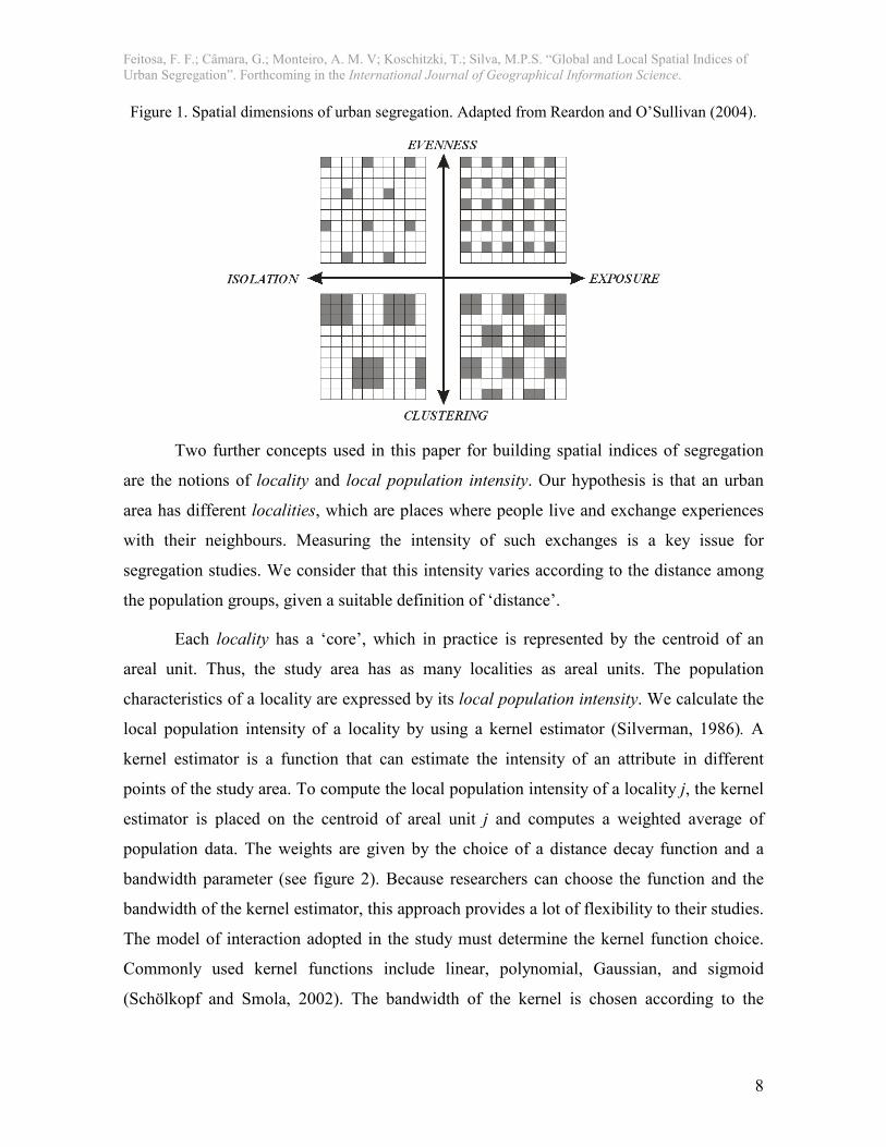
By arguing that segregation has no aspatial dimension, Reardon and O’Sullivan

(2004) reviewed Massey and Denton’s work. According to these authors, the difference

between the aspatial dimension evenness and the spatial dimension clustering is an effect of

data aggregation at different scales. The evenness degree at a certain scale of aggregation

(e.g., census tracts) is related to the clustering degree at a lower level of aggregation (e.g.,

blocks) (Reardon and O'Sullivan, 2004). Reardon and O’Sullivan combined both concepts

into the spatial evenness/clustering dimension, which refers to the balance of the

distribution of population groups. Centralization and concentration were considered

subcategories of the spatial evenness/clustering dimension. Reardon and O’Sullivan

conceptualized the dimension exposure as explicitly spatial. They proposed the spatial

exposure/isolation dimension, which refers to the chance of having members from

different groups (or the same group, if we consider isolation) living side-by-side (Reardon

and O'Sullivan, 2004).

Our work relies on Reardon and O’Sullivan’s dimensions of segregation and builds

spatial indices of segregation for each of them. Figure 1 presents a diagram where Reardon

and O’Sullivan’s dimensions are illustrated.


8

Figure 1. Spatial dimensions of urban segregation. Adapted from Reardon and O’Sullivan (2004).

Two further concepts used in this paper for building spatial indices of segregation

are the notions of locality and local population intensity. Our hypothesis is that an urban

area has different localities, which are places where people live and exchange experiences

with their neighbours. Measuring the intensity of such exchanges is a key issue for

segregation studies. We consider that this intensity varies according to the distance among

the population groups, given a suitable definition of ‘distance’.

Each locality has a ‘core’, which in practice is represented by the centroid of an

areal unit. Thus, the study area has as many localities as areal units. The population

characteristics of a locality are expressed by its local population intensity. We calculate the

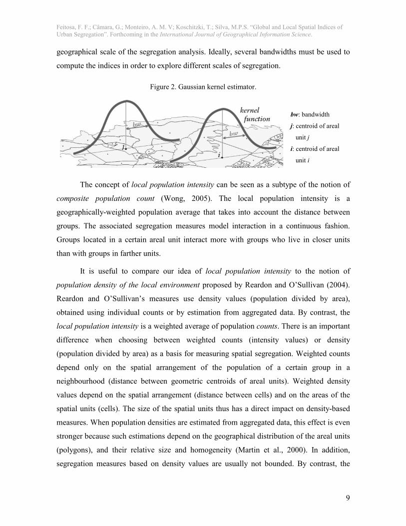
local population intensity of a locality by using a kernel estimator (Silverman, 1986). A

kernel estimator is a function that can estimate the intensity of an attribute in different

points of the study area. To compute the local population intensity of a locality j, the kernel

estimator is placed on the centroid of areal unit j and computes a weighted average of

population data. The weights are given by the choice of a distance decay function and a

bandwidth parameter (see figure 2). Because researchers can choose the function and the

bandwidth of the kernel estimator, this approach provides a lot of flexibility to their studies.

The model of interaction adopted in the study must determine the kernel function choice.

Commonly used kernel functions include linear, polynomial, Gaussian, and sigmoid

(Schölkopf and Smola, 2002). The bandwidth of the kernel is chosen according to the


9

geographical scale of the segregation analysis. Ideally, several bandwidths must be used to

compute the indices in order to explore different scales of segregation.

Figure 2. Gaussian kernel estimator.

bw: bandwidth

j: centroid of areal

unit j

i: centroid of areal

unit i

The concept of local population intensity can be seen as a subtype of the notion of

composite population count (Wong, 2005). The local population intensity is a

geographically-weighted population average that takes into account the distance between

groups. The associated segregation measures model interaction in a continuous fashion.

Groups located in a certain areal unit interact more with groups who live in closer units

than with groups in farther units.

It is useful to compare our idea of local population intensity to the notion of

population density of the local environment proposed by Reardon and O’Sullivan (2004).

Reardon and O’Sullivan’s measures use density values (population divided by area),

obtained using individual counts or by estimation from aggregated data. By contrast, the

local population intensity is a weighted average of population counts. There is an important

difference when choosing between weighted counts (intensity values) or density

(population divided by area) as a basis for measuring spatial segregation. Weighted counts

depend only on the spatial arrangement of the population of a certain group in a

neighbourhood (distance between geometric centroids of areal units). Weighted density

values depend on the spatial arrangement (distance between cells) and on the areas of the

spatial units (cells). The size of the spatial units thus has a direct impact on density-based

measures. When population densities are estimated from aggregated data, this effect is even

stronger because such estimations depend on the geographical distribution of the areal units

(polygons), and their relative size and homogeneity (Martin et al., 2000). In addition,

segregation measures based on density values are usually not bounded. By contrast, the


10

spatial segregation based on weighted counts proposed in this paper will always be

bounded from zero (0) to one (1) and are easier to interpret.

4 Global spatial indices of urban segregation

This section describes our proposed indices for measuring urban segregation on a global

scale. Based on the notion of local population intensity, we propose four new indices:

(a) the generalized spatial dissimilarity index )(mD(

, which is a measure of how the

population of each locality differs, on average, from the population composition as a

whole;

(b) the spatial exposure index *),( nmP

( that measures the potential contact between the

population groups m and n;

(c) the spatial isolation index mQ(

that measures the potential contact between people

belonging to the same population group; and

(d) the spatial neighbourhood sorting index ISN(, which measures the population

disparities between different localities of the study area.

The generalized spatial dissimilarity index )(mD(

, the spatial exposure index *),( nmP

(,

and the spatial isolation index mQ(

are more suitable for studies using categorical data, such

as those focused on racial or ethnical segregation. The spatial neighbourhood sorting index

ISN( is more suitable for socio-economic studies based on continuous data such as income

segregation.

All the spatial indices proposed in this paper require estimating the local population

intensity of all the localities of the city. The local population intensity of a locality j ( jL()

expresses its population characteristics:

( )∑=

=J

j

jj NkL1

(, (1)

where Nj is the total population in areal unit j; J is the total number of areal units in the

study area; and k is the kernel estimator which estimates the influence of each areal unit


11

on the locality j. We can calculate the local population intensity of group m in the locality j

( jmL(

) by replacing the total population in areal unit j (Nj) with the population of group m in

areal unit j (Njm) in equation (1):

( )∑=

=J

j

jmjm NkL1

(. (2)

4.1 The generalized spatial dissimilarity index

The generalized spatial dissimilarity index )(mD(

is a spatial version of the generalized

dissimilarity index )(mD developed by Sakoda (1981). The D(m) index is a measure of

how population proportions of each areal unit differs, on average, from the population

composition of the whole study area. Our spatial version of the generalized dissimilarity

index considers localities instead of areal units. The index measures the average difference

of the population composition of the localities from the population composition of the

urban area as a whole. Given a set of population groups, the generalized spatial

dissimilarity index )(mD(

captures the dimension evenness/clustering. The formula of

)(mD(

is:

mjm

J

j

M

m

j

NI

NmD ττ −=∑∑

= =

((

1 1 2)( (3)

where

( )( )∑=

−=M

m

mmI1

1 ττ and j

jm

jmL

L(

(

(=τ . (4) (5)

In equations (3) and (4), N is the total population of the city; Nj is the total

population in areal unit j; mτ is the proportion of group m in the city; jmτ(

is the local

proportion of group m in locality j; J is the total number of areal units in the study area; and

M is the total number of population groups. In equation (5), jmL(

is the local population

intensity of group m in locality j; and jL( is the local population intensity of locality j.


12

The index )(mD(

varies from 0 to 1, where 0 stands for the minimum degree of

evenness and 1 for the maximum degree. It is important to recognize the difference

between )(mD and )(mD(

. The aspatial dissimilarity index D(m) uses the proportion of

group n in the areal unit j instead of the local proportion jmτ(

of group m in locality j used in

)(mD(

. Therefore, the aspatial index )(mD does not measure the intensity of the interaction

across boundaries of areal unit j. By contrast, the spatial index )(mD(

is sensitive to the local

interaction. As an example, consider a mixed multiracial community where the census

tracts have been designed to be as homogeneous as possible in terms ethnicity. In this case,

the aspatial index might point out a high value of dissimilarity, whereas the spatial index

might be significantly lower and reflect the interaction between groups through the census

tract boundaries.

4.2 The spatial exposure and isolation indices

The spatial exposure index *),( nmP

( and the spatial isolation index mQ

( are spatial versions of

the exposure/isolation indices proposed by Bell (1954). These indices capture the

dimension exposure/isolation. Given two population groups in an urban area, we propose

the spatial exposure index of group m to group n ( *),( nmP

(), which measures the average

proportion of group n in the localities of each member of group m:

=∑

= j

jnJ

j m

jm

nmL

L

N

NP (

((

1

*),( , (6)

where Njm is the population of group m in areal unit j; Nm is the population of group m in

the study region; jnL(

is the local population intensity of group n in locality j; and jL( is the

local population intensity of locality j.

The index *),( nmP

( expresses the potential contact between the two population groups,

and ranges from 0 (minimum exposure) to 1 (maximum exposure). It is important to point

out the difference between *),( nmP

( and its aspatial version *

),( nmP . The aspatial index *),( nmP

uses the proportion of group n in the areal unit j and cannot capture the intensity of the

interaction between neighbouring areal units. By contrast, the spatial index *),( nmP

( is


13

sensitive to the interaction across areal boundaries. Even if an areal unit has a small internal

proportion of group n, the exposure index *),( nmP

( may still be high depending on the

proportion of individuals of group n in its neighbours. For example, a predominantly Black

areal unit with a low proportion of Hispanics inside may still present a high exposure index

between both groups, if its neighbourhood is mainly Hispanic.

Given one population group in an urban area, the spatial isolation index of group m

( mQ(

) is a particular case of the exposure index that expresses the exposure of group m to

itself:

=∑

= j

jmJ

j m

jm

mL

L

N

NQ (

((

1

, (7)

where jmL(

is the local population intensity of group m in locality j and the other equation

parameters are as in equation (6). The isolation index measures the average proportion of

group m in the localities of each member of the same group, and it varies from 0 (minimum

isolation) to 1 (maximum isolation).

The results of the exposure/isolation indices depend on the overall composition of

the city. For example, the exposure index of group m to group n ( *),( nmP

() usually will have

higher values if the proportion of group n in the city is high. In this case, it is more likely

that individuals from group n interact with other groups. Because of this property, the

exposure index is asymmetric, in other words, *),( nmP

( is not the same as *

),( mnP(

, except if the

city has the same proportion of people belonging to the groups m and n.

4.3 The spatial neighbourhood sorting index

The spatial neighbourhood sorting index ISN( is a spatial version of the neighbourhood

sorting index NSI (Jargowsky, 1996, Rodríguez, 2001), which is a variance-based measure

that captures the dimension evenness/clustering. The neighbourhood sorting index NSI has

the advantage of considering the original distribution of continuous data and, therefore, it is

suitable for socio-economic segregation studies based on data such as income. Considering

a continuous variable X, the NSI relies on the fact that the total variance of X in the city is

the sum of the between-area variance and the intra-area variance of X:


14

22between

2

intratotal σσσ += . (8)

The NSI is the ratio of the between-area variance of X ( 2betweenσ ) to the total variance

of X ( 2totalσ ). It is possible to build a spatial version of the NSI index. The idea of a spatial

NSI is to evaluate how much of the variance between the different localities contributes to

the total variance of the variable X. A greater contribution of the variance between localities

to the total variance expresses a smaller chance of interaction among the different

population groups and therefore a greater segregation between these groups. The proposed

spatial version of NSI ( ISN() represents the proportion of the variance between the different

localities ( 2betweenσ( ) that contributes to the total variance of X ( 2

totalσ( ) in the city:

2

2

total

betweenISNσσ(

((= . (9)

The variance of X between the different localities of the city is:

( )

∑

∑

=

=

−

=J

j

j

J

j

jj

between

L

XXL

1

1

22

2

(

(((

(σ , (10)

where

∑=

=M

m

mjmj XX1

τ((

and

∑

∑

=

==J

j

j

J

j

jj

L

XL

X

1

1

)(

(

((

( . (11)(12)

In equations (10) and (12), jL( is the local population intensity of locality j; J is the

total number of areal units in the study area; jX(

is the weighted average of X considering

the local proportion of all groups in the locality j; and X(

is the weighted average of jX(

in

the city. In equation (11), jmτ(

is the local proportion of group m in locality j; mX is the

value of X for group m; and M is the number of groups in the city.

The total variance of X in the city, considering the different localities, is:

∑=

−=M

m

mmtotal XX1

22 )((

(( τσ , (13)


15

where mτ(

is the proportion of group m in the city, considering the local population intensity

of all localities. Like the other indices, the ISN( varies from 0 to 1: the value 0 is the

minimum degree of segregation, and the value 1 represents the maximum degree.

5 Local spatial indices of urban segregation

The measures introduced until now - )(mD(

, *),( nmP

(, mQ(

and ISN( - represent global indices,

which summarize the segregation degree of the entire city. However, segregation is a

spatially variant process (Wong, 2002): a city may have areas with a significant degree of

segregation that global indices are not able to capture. This issue is especially important in

large urban areas, which have complex spatial patterns of segregation. To detect the local

variability of the phenomenon, local indices have been used in segregation studies (Wong,

1996, Wong, 1998b, Wong, 2002, Wong, 2003). Regarding the traditional measures, the

entropy diversity index (White, 1986) is able to capture local aspects of segregation in its

original form. Wong (1996) generated local measures by decomposing the dissimilarity

index D and its multi-group version D(m). In order to consider spatial parameters in local

analyses, Wong (2002) modified the entropy diversity index and proposed a set of spatial

local indices.

This paper proposes new local indices of segregation by decomposing the global

indices )(mD(

, *),( nmP

( and mQ

(. These local indices show how much each locality contributes

to the global segregation measure of a city. We can display these indices as maps and

identify the most critical areas. The formula of the local version of the spatial dissimilarity

index )(mD(

, which we refer as )(md j

(, is:

∑=

−=M

m

mjm

j

jNI

Nmd

1 2)( ττ(

( , (14)

where the equation parameters are the same as in equation (3).

Similarly, the local version of the exposure index of group m to group n ( *),( nmj

p(

) is:

=

j

jn

m

imnm

L

L

N

Np

j(

(

(*),(

, (15)


16

where the equation parameters are the same as in equation (6).

We calculate the local version of the isolation index of group m ( mjq(

) by replacing

jnL(

with the local population intensity of the group m in locality j ( jmL(

). Unlike the other

indices, the ISN( does not allow the generation of local indices from the approach

presented in this section.

6 Validation of spatial indices of segregation

Although the proposed measures have an established meaning, it is hard to interpret the

magnitude of the values obtained from their computation: do they indicate a segregated

population distribution? This issue is inherent to all segregation measures – aspatial or

spatial – since their values are quite sensitive to the scale of the data. Indices computed for

smaller areal units tend to present higher values than indices computed for larger areal

units. This is called the ‘grid problem’ (White, 1983). Since smaller areal units usually

present a more homogeneous distribution, this problem is expected and has been

empirically observed in several studies (Wong, 1997, Wong, 2004, Sabatini et al., 2001,

Rodríguez, 2001).

In the case of spatial measures that allow researchers to specify their own definition

of neighbourhood, as the ones proposed in this paper, this scale variability is also related to

the bandwidth used in the computation of the measures. An index computed with a small

bandwidth will have higher values than one that is computed with a large bandwidth. Since

the indices calculated for distinct bandwidths have different ranges of magnitude, there is

no fixed threshold that asserts whether the results indicate a segregated situation. In order to

provide an insight in this direction, we propose the use of a random permutation test

(Anselin, 1995) for the measures presented in this paper. By applying this test, it is possible

to verify if the spatial arrangement of the areal units in the study area promotes segregation

among different population groups.

In the permutation test, we randomly permute the population data of areal units to

produce spatially random layouts with the same data as observed. For each random layout,

we calculate local population intensity values for all localities and compute the segregation


17

index. The spatial permutation of original data among the areal units generates very

different values of local population intensities and therefore different values of segregation

indices.

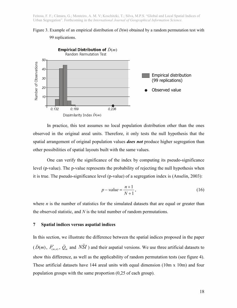
From the segregation indices computed for each random layout, one can build an

empirical distribution of the index to which the segregation index computed for the original

dataset will be compared. Figure 3 presents the example of an empirical distribution of the

dissimilarity index )(mD(

built with 99 replications. The empirical distribution (grey bars in

figure 3) ranges from 0,132 to 0,169 while the value of the index computed for the original

data is 0,236 (black point). This shows that the original population distribution of areal

units represents an arrangement with a higher segregation level than randomly generated

arrangements.

One may argue that it is practically impossible to find an empirical example where

the same would not be observed, since the population distribution of real cities will always

be more segregated than a randomly generated one. This may be true for the dissimilarity

)(mD(

or isolation index mQ(

, but the application of the test is particularly interesting for the

exposure index *),( nmP

(. It is feasible to find real examples where the degree of exposure

between two population groups is lower, equal or higher than the ones obtained by

permuting the original values.


18

Figure 3. Example of an empirical distribution of D(m) obtained by a random permutation test with

99 replications.

In practice, this test assumes no local population distribution other than the ones

observed in the original areal units. Therefore, it only tests the null hypothesis that the

spatial arrangement of original population values does not produce higher segregation than

other possibilities of spatial layouts built with the same values.

One can verify the significance of the index by computing its pseudo-significance

level (p-value). The p-value represents the probability of rejecting the null hypothesis when

it is true. The pseudo-significance level (p-value) of a segregation index is (Anselin, 2003):

1

1

++

=−N

nvaluep , (16)

where n is the number of statistics for the simulated datasets that are equal or greater than

the observed statistic, and N is the total number of random permutations.

7 Spatial indices versus aspatial indices

In this section, we illustrate the difference between the spatial indices proposed in the paper

( )(mD(

, *),( nmP

(, mQ(

and ISN(

) and their aspatial versions. We use three artificial datasets to

show this difference, as well as the applicability of random permutation tests (see figure 4).

These artificial datasets have 144 areal units with equal dimension (10m x 10m) and four

population groups with the same proportion (0,25 of each group).

Empirical distribution (99 replications)

Observed value

)(mD(

)(mD(


19

In each dataset, the distribution of population groups is different. Dataset A is a case

of extreme segregation, where each areal unit has just individuals of one group and the

units characterized by the same group are clustered. In dataset B, each areal unit has also

just individuals of one group, but the distribution of these units is well-balanced. Dataset C

is a case of extreme integration, where each areal unit has the same population composition

of the entire set.

Figure 4. Artificial datasets.

Group 1

Group 2

Group 3

Group 4

DATASET A DATASET B DATASET C

We calculated the aspatial indices D(m) and NSI and the spatial indices )(mD(

and

ISN( for each dataset (see table 1). We used Gaussian kernel estimators with bandwidth of

10m and 30m for computing the spatial indices )(mD(

and ISN(. To calculate the averages

and variances required in NSI and ISN(, we assigned a different numerical value to each

group (0 to 3). For datasets A and B, we validated the spatial indices by a random

permutation test with 99 replications. The same procedure was not possible for the dataset

C because all units have the same data and random permutation would not change the

spatial arrangement.


20

Table 1. Comparison between )(mD , )(mD(

, NSI and ISN(

.

Generalized Dissimilarity Indices - )(mD and )(mD(

Aspatial Gaussian kernel, bandwidth 10m

Gaussian kernel, bandwidth 30m

)(mD p-value )(mD(

p-value )(mD(

p-value

Dataset A 1 - 0.86 0.01 0.54 0.01

Dataset B 1 - 0.05 1 0.04 1

Dataset C 0 - 0 - 0 -

Neighbourhood Sorting Indices - NSI and ISN(

Aspatial Gaussian kernel, bandwidth 10m


NSI p-value ISN(

p-value ISN(

p-value

Dataset A 1 - 0.82 0.01 0.39 0.01

Dataset B 1 - 0.007 1 0.001 1

Dataset C 0 - 0 - 0 -

As seen in table 1, although dataset A has a much more segregated distribution than

dataset B, the aspatial measures point out both datasets as examples of maximum

segregation (D(m) = 1 and NSI = 1). Such result illustrates the ‘checkerboard problem’: if

only individuals of the same group occupy the areal units, the result of aspatial indices will

be always extreme, regardless the spatial arrangement of the units. Because they consider

neighbourhood relations, the spatial indices allow distinguishing between dataset A and B.

The spatial indices for dataset A have high values which are significant (p-value = 0.01)

and the spatial indices for dataset B have low values which are nonsignificant (p-value =

1).

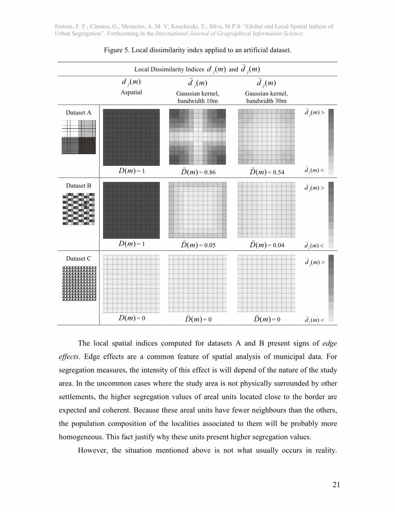
To promote further insight into the problem of estimating spatial segregation, we

have calculated the )(md j

( local index of dissimilarity for datasets A, B, and C, as shown in

figure 5. The spatial variation of )(md j

( allows identifying the most segregated areas. In

dataset A, the most segregated units are close to the borders, whereas the most integrated

units are in the centre, where different groups are close to one another.


21

Figure 5. Local dissimilarity index applied to an artificial dataset.

Local Dissimilarity Indices )(md j and )(md j

(

)(md j

Aspatial

)(md j

(


)(md j

(


Dataset A

)(mD = 1 )(mD

(= 0.86 )(mD

(= 0.54

Dataset B

)(mD = 1 )(mD

(= 0.05 )(mD

(= 0.04

Dataset C

)(mD = 0 )(mD

(= 0 )(mD

(= 0

The local spatial indices computed for datasets A and B present signs of edge

effects. Edge effects are a common feature of spatial analysis of municipal data. For

segregation measures, the intensity of this effect is will depend of the nature of the study

area. In the uncommon cases where the study area is not physically surrounded by other

settlements, the higher segregation values of areal units located close to the border are

expected and coherent. Because these areal units have fewer neighbours than the others,

the population composition of the localities associated to them will be probably more

homogeneous. This fact justify why these units present higher segregation values.

However, the situation mentioned above is not what usually occurs in reality.

>)(md j

(

>

<)(md j

(

<

>)(md j

(

>

<)(md j

(

<

>)(md j

(

>

<)(md j

(

<


22

People who live close to the boundaries of a city interact with people who live in the

neighbouring city. In this case, the higher segregation values at the border are unrealistic

since they are a merely consequence of the lack of data beyond city borders. We consider

that the impact of these edge effects could only be minimized if data for neighbouring

cities would be available. If it is not possible, the analyst must be aware that the

segregation measures are mostly appropriate for inner-city analysis.

Figure 5 also shows the result of using different bandwidths for the kernel

estimators. As mentioned in section 6, larger bandwidths produce lower indices of

segregation. The larger the bandwidth, the more the localities assimilate the population

characteristics of a greater number of tracts. The bandwidth of the spatial index is therefore

associated with the extent of the neighbourhood influence in the study area. By using

different bandwidths, the proposed indices work as an exploratory tool for analysing

segregation at different scales.

Since segregation measures rely on the population composition of the areal units (or

localities) of a certain study area, the issue of scale is fundamental in any empirical analysis

about the phenomenon and has been addressed by several studies (Sabatini et al., 2001,

Sabatini, 2000, Torres, 2004, Rodríguez, 2001, Wong, 2004). It is feasible that different

scales of segregation present different trends along the years. Segregation can increase at a

certain scale and decrease at another one (Sabatini et al., 2001, Sabatini, 2000, Rodríguez,

2001, Torres, 2004). It is possible that negative impacts of segregation (e.g., violence or

unemployment) are stronger at a certain scale, while segregation at other scales can be even

associated to positive aspects (Sabatini et al., 2001, Sabatini, 2000).

There is no ‘right’ scale for analysing segregation. The analyst should observe the

phenomenon at different scales by choosing different bandwidths for the segregation

indices. The segregation indices proposed in the paper allow the use of neighbourhood

functions in different scales. The next section presents a case study that adopts different

bandwidths in the computation of the segregation measures.


23

8 A case study: São José dos Campos, Brazil

To illustrate the use of the proposed spatial indices of segregation, we applied them to an

empirical example of socio-economic urban segregation in the city of São José dos

Campos. The city had 532,711 inhabitants in the 2000 census, and is located in the State of

São Paulo, Brazil. São José dos Campos is a city with recent industrialization and is host to

most of the Brazilian aerospace sector. The city also has car manufacturers, an oil refinery,

and other traditional industries. São José dos Campos has the ninth highest GDP among

Brazilian cities, and a per capita GDP of US$ 10,715, nearly three times higher than the

country’s average. Nevertheless, the city also has a large quantity of poor and excluded

classes. Because most of the jobs in the industrial sector need skilled labour, there is a

sizable portion of the population that is excluded from the city’s economic wealth

(Genovez et al., 2003).

Since the 1950’s, São José dos Campos presented a large-scale segregation pattern

known as ‘Centre-Periphery’ (Caldeira, 2000, Torres et al., 2002). In other words, the city

was characterised by a strong contrast between the rich central area, legalized and well

equipped, and the poor outskirts, precarious and usually illegitimate.

However, economical and social changes that occurred in the 1980s introduced

changes in the dichotomous segregation pattern that has prevailed until then. The main

feature of this changing was the proliferation of “gated communities” for medium and high-

income families in different areas of the city, including poor neighbourhoods. This

phenomenon has been well documented in the literature about segregation in Latin

American cities (Caldeira, 2000, Sabatini et al., 2001, Villaça, 1998) and is related to a

decrease in the scale of segregation1 (Sabatini et al., 2001). The growing of favelas in most

part of the cities, including the wealthy central area, is another process that has also

promoted the decrease in the scale of segregation.

Villaça (1998) asserts that despite the spreading of gated communities and favelas -

processes that establish smaller distances among different social groups - it is important to

observe the city in relation to its macrosegregation. The process of self-segregation of

1 In this context, the term “scale” refers to the proximity between elements in space, and not to the

cartographic meaning of the word.


24

medium and high-income groups follows a certain direction of territorial expansion starting

from the central area of the city. In addition, cities still attract new contingents of poor

families that locate in far areas of the cities and establish large homogeneous settlements. It

is possible to observe these both trends in São José dos Campos, which are related to an

increase in the scale of segregation.

By this brief review, it is possible to note that the segregation pattern of São José

dos Campos, as well other Latin American cities, has become more complex and ruled by

antagonistic forces that deal with different scales of segregation. This complexity has

operational consequences and points out the importance of measuring segregation in

different scales. This study case shows the potential of the proposed measures by using

kernel estimators with several different bandwidths to compute the indices.

Because the most important aspects to portray segregation in São José dos Campos

are socio-economic, we selected the attributes ‘family head income’ and ‘family head

education’ to represent the socio-economic status of families. The Brazilian Census

provides these variables in artificially built intervals of income and years of study rather

than the values for individuals (see table 2). This fact represents a limitation for the use of

these variables, since they are not truly categorical (suitable for the indices )(mD(

, *),( nmP

(

and mQ(

) and also not truly continuous (suitable for the index ISN(). However, this

drawback is an outcome of real challenges concerning Brazilian Census data: income and

education are not provided as continuous variables and socioeconomic categorical

variables, such as occupation, are only collected by sample. Because this is a common

problem to which many researchers have to deal, we decided to use the available variables

and demonstrate how to extract meaningful segregation analyses from them.

Table 2. Groups of population considered in the analyses. Family head income - Groups Family head education - Groups

• No income. • Income inferior than 2 minimum wages*. • Income between 2 and 5 minimum wages. • Income between 5 and 10 minimum wages. • Income between 10 and 20 minimum wages. • Income greater than 20 minimum wages.

• 0 or less than 1 year of schooling. • 1 to 3 years of schooling. • 4 to 7 years of schooling. • 8 to 10 years of schooling • 11 to 14 years of schooling. • 15 years of schooling or more.

*Minimum wage is the lowest level of work compensation secured by law. The Brazilian minimum wage was CR$ 17.000 per month (U$ 50) in 1991 and R$ 151,00 per month (U$ 85) in 2000.


25

The data about family head income and education was derived from the 1991 and

2000 Census. The Census records the number of family heads in each of the groups

presented in table 2. Figure 6 shows the composition of population groups in São José dos

Campos during the years 1991 and 2000 according to the variables family head income and

education. The graphics of figure 6 reveals that an improvement in socio-economic

indicators, mainly education, has occurred during the period 1991-2000.

Figure 6. Population composition according to the variables family head income and education

(1991 and 2000).

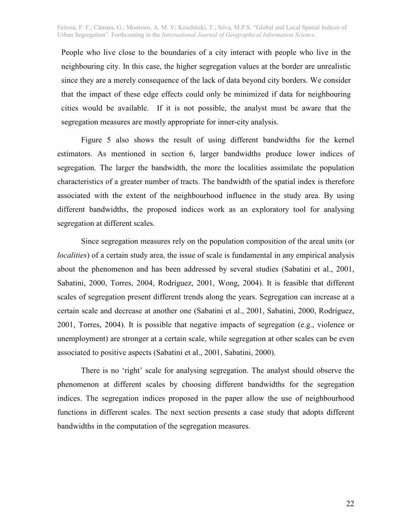
Figure 7 shows summary maps of the income distribution in the years 1991 and

2000. The maps presented in figure 7 depict clear signs of a ‘Centre-Periphery’ pattern in

1991, where higher-income groups are close to the centre, lower-income groups are located

in far peripheries, and groups with income between 2 and 10 minimum wages are in

intermediary areas. The 2000 map shows a more complex segregation pattern. The high-

income families have expanded from the centre towards the western part of the city. The

education of family heads has a similar spatial distribution to the one presented in figure 7.


26

Figure 7. Predominance of income groups in São José dos Campos, 1991 and 2000.

Income of Family Heads

1991 2000

The variables ‘family head income’ and ‘education’ are aggregated by Census

tracts, whose boundaries change over time. To compare the results for 1991 and 2000, we

produced a single partition of space that combines both geometries. The resulting data

comprised 421 areal units. Small polygons represent areas with a high density of families,

while large polygons comprise areas with lower population density.

Table 3 presents the indices of socio-economic segregation of São José dos Campos

in the years 1991 and 2000. To compute the ISN(

index (neighbourhood sorting), it was

necessary to estimate the variance of the chosen variables, which is not available in tract-

level census data. We adopted a method proposed by Jargowsky (1996), which is based on

assumptions about the distribution of the heads of families. After several tests, the author

has assumed linear distributions for lower intervals and Pareto distributions for the intervals

above the mean of the attribute in the city.

Predominance of heads of family with:

No income or income inferior than 2 MW

Income between 2 and 10 MW

Income greater than 10 MW


27

Table 3. Indices computed for São José dos Campos data.

Dimension Spatial Evenness/Clustering:

Symbol Spatial segregation index

)(mD(

Generalized spatial dissimilarity index (for income and education).

ISN( Spatial neighbourhood sorting index (for income and education).

Dimension Spatial Exposure/Isolation:

Symbol Spatial segregation index

20>Q( Spatial isolation index of family heads with income greater than 20 MW.

15>Q( Spatial isolation index of family heads with 15 years of schooling or more.

0Q( Spatial isolation index of family heads with no income.

*)20,0( >P

( Spatial exposure index of family heads with no income to family heads with income greater

than 20 minimum wages (MW).

Gaussian kernel estimators with eight different bandwidths (from 200m to 4400m)

were used to define the localities and compute their local population intensity. The

aspatial versions of the indices were also computed. To calculate the pseudo-significance

level of the spatial indices, we produced 99 random datasets (same attributes, different

locations) and calculated the indices in each case. Figures 8 and 9 present the results of

segregation indices for the dimension evenness/clustering ( )(mD(

and ISN(). The graphics

present indices computed for income and education indicators and with different

bandwidths. They also show the results of the aspatial indices )(mD and NSI .


28

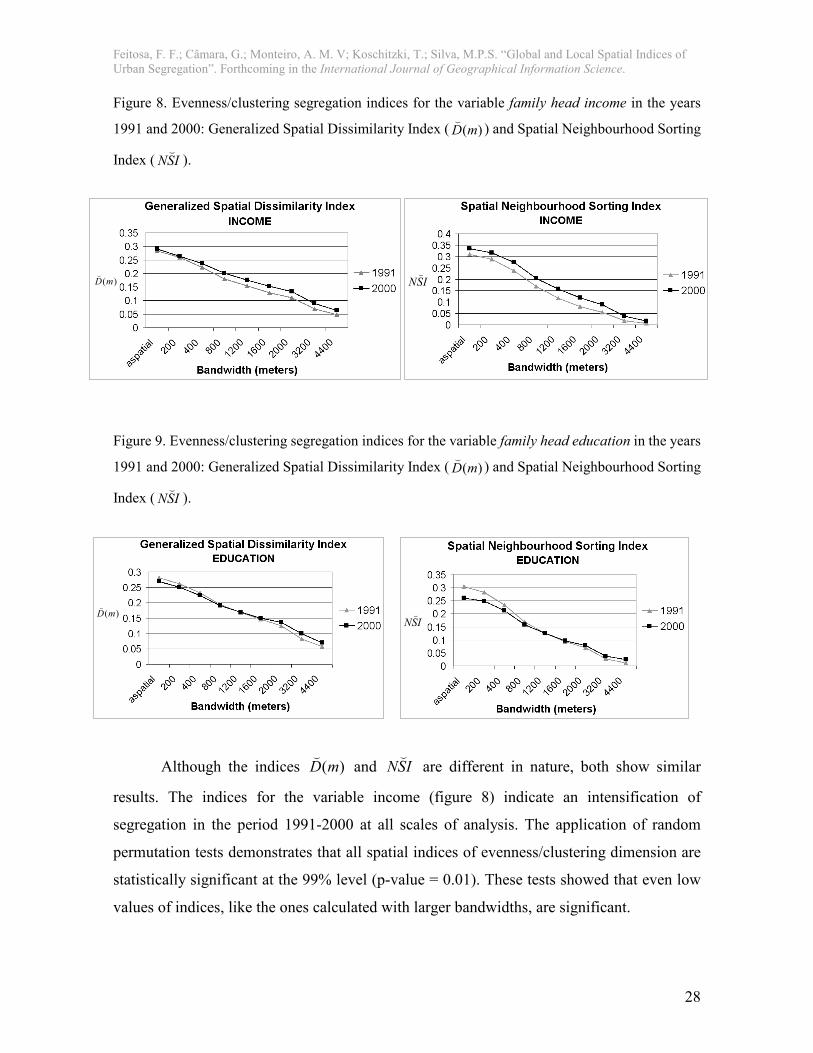
Figure 8. Evenness/clustering segregation indices for the variable family head income in the years

1991 and 2000: Generalized Spatial Dissimilarity Index ( )(mD(

) and Spatial Neighbourhood Sorting

Index ( ISN().

Figure 9. Evenness/clustering segregation indices for the variable family head education in the years

1991 and 2000: Generalized Spatial Dissimilarity Index ( )(mD(

) and Spatial Neighbourhood Sorting

Index ( ISN().

Although the indices )(mD(

and ISN( are different in nature, both show similar

results. The indices for the variable income (figure 8) indicate an intensification of

segregation in the period 1991-2000 at all scales of analysis. The application of random

permutation tests demonstrates that all spatial indices of evenness/clustering dimension are

statistically significant at the 99% level (p-value = 0.01). These tests showed that even low

values of indices, like the ones calculated with larger bandwidths, are significant.

)(mD(

ISN(

)(mD(

ISN(


29

The evenness/clustering indices computed for education (figure 9) show different

results when compared to the indices computed for income. Segregation in education for

the period 1991-2000 presents different trends according to the scale of analysis. Indices

computed with smaller bandwidths showed a lower degree of segregation in 2000 than in

1991. Indices computed with larger bandwidths indicate an increase in segregation during

the period. The result is related to the improvement of education indicators that occurred in

the period 1991-2000. The improvement in education levels has not yet resulted in a

corresponding gain in income. Thus, many heads of family with higher levels of education

now live in neighbourhoods that are also occupied by groups with lower levels of

education.

Additional insight into segregation patterns is provided by computing local indices

that are suitable for visualization as maps that show the degree of segregation in different

parts of the city. We computed the local dissimilarity index )(md j

( for the 1991 and 2000

data sets. Figure 10 presents the change map of the local index )(md j

( computed for a local

scale (bandwidth of 400m) for the variable education of family heads. The maps show that

segregation increased in the outskirts of the city, mainly in the western and southern

regions. Segregation decreases in dense areas of the city, such as downtown. By these

results, it is possible to assert that the increasing diversity of these dense areas are

responsible for the decreasing of segregation pointed out by the global indices )(mD(

computed for lower scales. This example demonstrates the importance of analysing

segregation using global and local indices in a complementary manner.


30

Figure 10. Change map 1991-2000: local dissimilarity index, bandwidth of 400 m, computed for the

variable education of family heads

Change Map 1991-2000: Local Dissimilarity Index )(md j

(

Education of family heads - Gaussian kernel, bandwidth = 400m

Figure 11 presents maps of the local index )(md j

( computed for a larger scale

(bandwidth of 3200m), considering the variable education of family heads. In these maps,

we identify macrosegregation patterns in the city, which means, groups of neighbourhoods

where social groups are clustered (Villaça, 1998). Peripheral clusters of low-education

family heads in the northern, eastern and southern region are encircled in grey in figure 11.

These clusters have different types of occupation. The southern cluster has social housing

built by the City. The eastern cluster contains several settlements, mainly illegal and

characterized by self-constructed housing. The northern cluster corresponds to an area with

sparse occupation with rural characteristics. Figure 11 also shows a cluster encircled in

black that is predominantly occupied by high-education family heads. The maps show a

remarkable increase in the segregation of this high-income clustering in the period 1991-

2000. The local segregation indices maps are susceptible to edge effects, which are more

intense with the increasing in the bandwidths.

LEGEND

)(md j

( 1991 > )(md j

( 2000

)(md j

( 2000 > )(md j

( 1991


31

Figure 11. Local dissimilarity index maps (1991 and 2000), bandwidth of 3200m, computed for the

variable education of family heads.

Local Dissimilarity Index

Gaussian kernel, bandwidth = 3200m

1991 - )(mD(

=0.08 2000 - )(mD(

=0.10

Figure 12 presents the aspatial isolation index ( mQ ) and the spatial isolation indices

( mQ(

) for the highest income and education groups, computed for several bandwidths. The

indices were computed for family heads with income greater than 20 MW ( 20>Q(

and 20>Q )

and family heads with 15 years of schooling or more ( 15>Q(

and 15>Q ). Because the results

of isolation indices vary according to the proportion of population groups in the city, we

also provide this information (τ).

)(md j

(


32

Figure 12. Isolation indices for the highest income and education groups: family heads with income

greater than 20 MW ( 20>Q(

and 20>Q ) and family heads with 15 years of schooling or more ( 15>Q(

and 15>Q ).

The indices computed for family heads with the highest income and education

levels ( 20>Q(

and 15>Q(

) present much higher values than the proportion of the group in the

city. This feature was particularly evident in the variable income. In 2000, the value of the

isolation index of high-income family heads ( 20>Q(

) computed with a bandwidth of 400m

was 0.28, while the proportion of this group in the city was only 0.07. The average

proportion of the highest-income group in the localities where the members of this same

group live is four times higher than the groups’ proportion in the city as a whole. The

increase in the isolation indices of this group during the period 1991-2000 was much

greater than the variability of its proportion. These results lead to the assumption that high-

income family heads had a significant role in the increment of segregation in São José dos

Campos.

Figure 13 shows the maps of the local isolation indices of family heads with income

greater than 20 MW during the years 1991 and 2000 (bandwidth of 400m). The figure

confirms an increase in the local isolation indices of high-income family heads in the

western region (encircled in black). This result suggests that the increase in the isolation of

this region was the main promoter of the increment of the global isolation index (from 0.20

in 1991 to 0.28 in 2000, considering the bandwidth of 400m).

20>Q( 15>Q

(


33

Figure 13. Local isolation index maps - family heads with income greater than 20 minimum wages

(1991 and 2000), bandwidth of 400m.

Isolation Index of family heads with income greater than 20 minimum wages

Gaussian kernel, bandwidth = 400m

1991 - 20>Q(

=0.20 2000 - 20>Q(

=0.28

To provide a comparison between spatial and aspatial indices of segregation, we

calculated local isolation and exposure indices for two different low-income areas of the

city. The first area is a favela located in downtown and surrounded by medium- and high-

income areas. The second area is settlement with social housing promoted by the State and

located in a poor homogeneous region at the periphery of the city. We decomposed aspatial

segregation indices to obtain local indices and computed them to both low-income areas.

We also computed spatial local indices with different bandwidths.

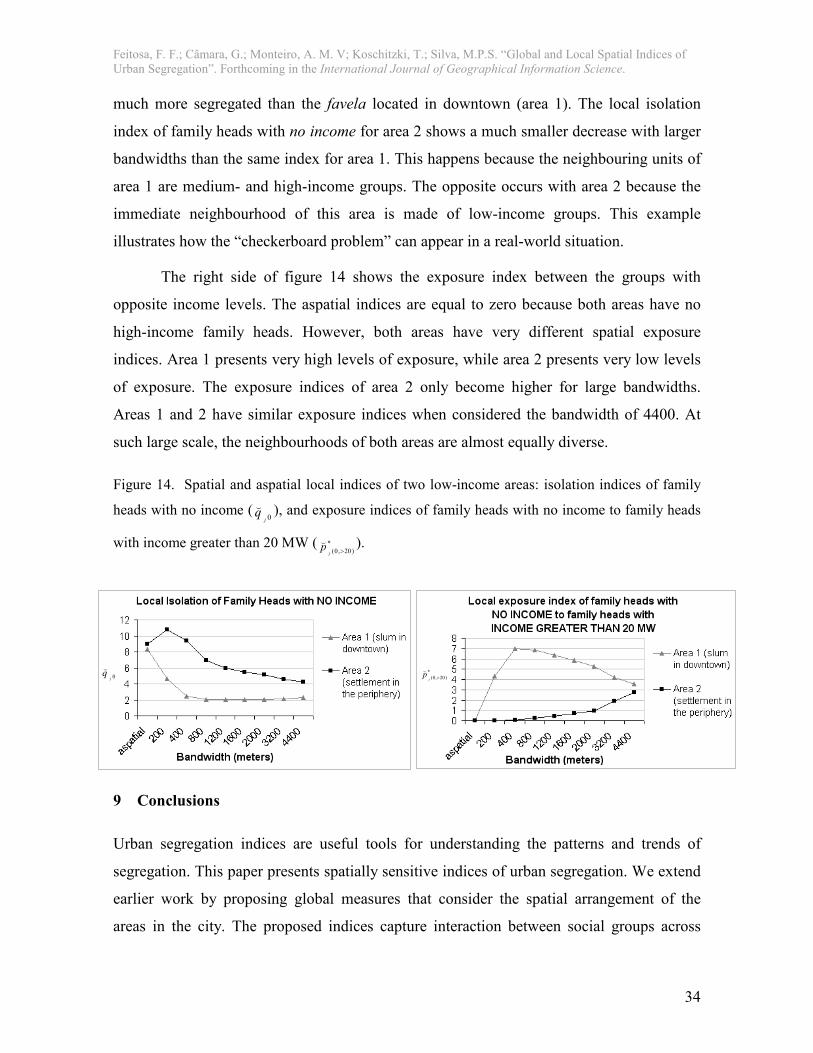
Figure 14 shows the results of the local indices for both low-income areas. The left

side presents isolation indices of family heads with no income. The right side presents

exposure indices of family heads with no income to family heads with income greater than

20 MW. According to the aspatial indices, both areas present similar degrees of segregation.

By contrast, the spatial indices point out that the settlement in the periphery (area 2) is

<>20jq(


34

much more segregated than the favela located in downtown (area 1). The local isolation

index of family heads with no income for area 2 shows a much smaller decrease with larger

bandwidths than the same index for area 1. This happens because the neighbouring units of

area 1 are medium- and high-income groups. The opposite occurs with area 2 because the

immediate neighbourhood of this area is made of low-income groups. This example

illustrates how the “checkerboard problem” can appear in a real-world situation.

The right side of figure 14 shows the exposure index between the groups with

opposite income levels. The aspatial indices are equal to zero because both areas have no

high-income family heads. However, both areas have very different spatial exposure

indices. Area 1 presents very high levels of exposure, while area 2 presents very low levels

of exposure. The exposure indices of area 2 only become higher for large bandwidths.

Areas 1 and 2 have similar exposure indices when considered the bandwidth of 4400. At

such large scale, the neighbourhoods of both areas are almost equally diverse.

Figure 14. Spatial and aspatial local indices of two low-income areas: isolation indices of family

heads with no income (0j

q( ), and exposure indices of family heads with no income to family heads

with income greater than 20 MW ( *)20,0( >j

p( ).

9 Conclusions

Urban segregation indices are useful tools for understanding the patterns and trends of

segregation. This paper presents spatially sensitive indices of urban segregation. We extend

earlier work by proposing global measures that consider the spatial arrangement of the

areas in the city. The proposed indices capture interaction between social groups across

*)20,0( >P

( 0jq( *

)20,0( >jp(


35

boundaries of areal units, by using the ideas of locality and local population intensity.

Interaction across boundaries is computed by a kernel estimator. The flexibility provided by

the choice of the parameters of the kernel estimator allows analysis on different scales, an

issue that is particularly important in studies of urban segregation. Because the proposed

approach is general, we can use it for extending other aspatial indices.

In addition, this paper presents local indices of segregation, which show the

intensity of segregation in different localities of the city. The local indices can be displayed

as maps that allow visualisation of segregation patterns. This paper also recommends the

use of a permutation test for the statistical validation of the indices. Although this test does

not support statements about the intensity of segregation, it provides a way for verifying if a

certain population distribution is segregated or not. It is also possible to apply permutation

tests to local indices and identify which areas inside the city present significant levels of

segregation.

With the purpose of evaluating the proposed indices, we applied them on an

artificial dataset and on a real case study in São José dos Campos. The study using the

artificial dataset showed the limitations of the aspatial indices compared to spatially

sensitive ones. The São José dos Campos case study showed that local indices are useful

for exploratory data analysis and visualisation. The flexibility provided by kernel estimators

was also demonstrated. By using different bandwidths, we could reveal patterns of

segregation on different scales. The spatial indices can also allow other types of analyses if

we use more complex kernel estimators, such as estimators that are able to consider

transport networks or obstacles.

References

ANSELIN, L., 1995, Local indicators of spatial association - LISA. Geographical Analysts, 27, pp. 93-115.

ANSELIN, L., 2003, GeoDa 0.9 User's Guide, pp. 82 (Urbana-Champaign: University of Illinois).

BELL, W., 1954, A probability model for the measurement of ecological segregation. Social Forces, 32, pp. 337-364.


36

CALDEIRA, T., 2000, City of walls: Crime, Segregation and Citizenship in Sao Paulo, pp. 487 (Berkeley: University of California Press).

DUNCAN, O. D. and DUNCAN, B., 1955, A methodological analysis of segregation indexes. American Sociological Review, 20, pp. 210-217.

FEITOSA, F. F., CÂMARA, G., MONTEIRO, A. M. V., KOSCHITZKI, T. and SILVA, M. P. S., 2004, Spatial measurement of residential segregation. In VI Brazilian Symposium on GeoInformatics, 22-24 Nov 2004, Campos do Jordão (Geneve: IFIP), pp.59-73.

GENOVEZ, P. C., MONTEIRO, A. M. V., CÂMARA, G. and FREITAS, C. C., 2003, Análise espacial da dinâmica de exclusão/Inclusão social em São José dos Campos (1991-

2000): Definição de áreas pilotos para planejamento e direcionamento de políticas

públicas, pp.47 (São José dos Campos: Instituto Nacional de Pesquisas Espaciais).

JAKUBS, J. F., 1981, A distance-based segregation index. Journal of Socio-Economic Planning Sciences, 61, pp. 129-136.

JARGOWSKY, P. A., 1996, Take the money and run: Economic segregation in U.S. metropolitan areas. American Journal of Sociology, 61, pp. 984-999.

MARTIN, D., TATE, N. J. and LANGFORD, M., 2000, Refining population surface models: Experiments with Northern Ireland Census Data. Transactions in GIS, 4, pp. 343-360.

MASSEY, D. S. and DENTON, N. A., 1987, Trends in the residential segregation of Hispanics, Blacks and Asians: 1970-1980. American Sociological Review, 52, pp. 802-824.

MASSEY, D. S. and DENTON, N. A., 1988, The dimensions of residential segregation. Social Forces, 67, pp. 281-315.

MASSEY, D. S. and DENTON, N. A., 1993, American apartheid: segregation and the making of the underclass, pp. 292 (Cambridge: Harvard University Press).

MORGAN, B. S., 1975, The segregation of socioeconomic groups in urban areas: A comparative analysis. Urban Studies, 12, pp. 47-60.

MORGAN, B. S., 1983, A temporal perspective on the properties of the index of dissimilarity. Environment and Planning A, 15, pp. 379-389.

MORRILL, R. L., 1991, On the measure of spatial segregation. Geography Research Forum, 11, pp. 25-36.

REARDON, S. and O'SULLIVAN, D., 2004, Measures of spatial segregation. Sociological Methodology, 34, pp. 121-162.


37

REARDON, S. F. and FIREBAUGH, G., 2002, Measures of multigroup segregation. Sociological Methodology, 32, pp. 33-67.

RODRÍGUEZ, J., 2001, Segregación residencial socioeconómica: que és?, cómo de mide?, que está pasando?, importa?, pp. 80 (Santiago de Chile: CELADE / United Nations).

SABATINI, F., 2000, Reforma de los mercados de suelo en Santiago, Chile: efectos sobre los precios de la tierra y la segregación residencial. EURE (Santiago), 26, pp. 49-80.

SABATINI, F., CÁCERES, G. and CERDA, J., 2001, Residential segregation pattern changes in main Chilean cities: Scale shifts and increasing malignancy. In International Seminar on Segregation in the City, 26-28 July 2001, Lincoln Institute of Land Policy, Cambridge. Available online at: www.lincolninst.edu/pubs/dl/615_sabatini_caceres_cerda.pdf (accessed 22 Aug 2005).

SAKODA, J., 1981, A generalized index of dissimilarity. Demography, 18, pp. 245-250.

SCHÖLKOPF, B. and SMOLA, A. J., 2002, Learning with Kernels : Support Vector Machines, Regularization, Optimization, and Beyond, pp. 626 (Cambridge, MA ; London: MIT Press).

SILVERMAN, B. W., 1986, Density estimation for statistics and data analysis, pp. 175 (London; New York: Chapman and Hall).

TORRES, H. G., 2004, Segregação residencial e políticas públicas: São Paulo na década de 1990. Revista Brasileira de Ciências Sociais, 19, pp. 41-56.

TORRES, H. G., MARQUES, E. C., FERREIRA, M. P. and BITAR, S., 2002, Poverty and space: Pattern of segregation in São Paulo. In Workshop on Spatial Segregation and Urban Inequality in Latin America, November, 15-16 (Austin, Texas).

TORRES, H. G. and OLIVEIRA, G. C., 2001, Primary education and residential segregation in the Municipality of São Paulo: a study using geographic information systems. In International Seminar on Segregation in the City, 26-28 July 2001, Lincoln Institute of Land Policy, Cambridge. Available online at: www.centrodametropole.org.br/pdf/torres_coelho.pdf (accessed 22 Aug 2005).

VILLAÇA, F., 1998, Espaço Intra-Urbano no Brasil, pp. 373 (São Paulo: Studio Nobel).

VILLAÇA, F., 2001, Segregation in the Brazilian Metropolis. In International Seminar on Segregation in the City, 26-28 July 2001, Lincoln Institute of Land Policy, Cambridge. Available online at: www.lincolninst.edu/pubs/dl/620_villaca.pdf (accessed 22 Aug 2005).

WHITE, M. J., 1983, The measurement of spatial segregation. American Journal of Sociology, 88, pp. 1008-1018.


38

WHITE, M. J., 1986, Segregation and diversity measures in population distribution. Population Index, 52, pp. 198-221.

WONG, D. W. S., 1993, Spatial indices of segregation. Urban Studies, 30, pp. 559-572.

WONG, D. W. S., 1996, Enhancing segregation studies in GIS. Computers, Environment and Urban Systems, 20, pp. 99-109.

WONG, D. W. S., 1997, Spatial dependency of segregation indices. The Canadian Geographer, 41, pp. 128-136.

WONG, D. W. S., 1998a, Measuring multiethnic spatial segregation. Urban Geography, 19, pp. 77-87.

WONG, D. W. S., 1998b, Spatial patterns of ethnic integration in the United States. Professional Geographer, 50, pp. 13-30.

WONG, D. W. S., 2002, Modeling local segregation: A spatial interaction approach. Geographical and Environmental Modelling, 6, pp. 81-97.

WONG, D. W. S., 2003, Spatial decomposition of segregation indices: a framework toward measuring segregation at multiple levels. Geographical Analysis, 35, pp. 179-194.

WONG, D. W. S., 2004, Comparing traditional and spatial segregation measures: a spatial scale perspective. Urban Geography, 1, pp. 66-82.

WONG, D. W. S., 2005, Formulating a general spatial segregation measure. The Professional Geographer, 57, pp. 285-294.

global and local spatial indices of urban segregation

Documents