Global and Planetary Change 77 (2011) 49–61

Contents lists available at ScienceDirect

Global and Planetary Change

j ourna l homepage: www.e lsev ie r.com/ locate /g lop lacha

Two-dimensional reconstruction of the Mediterranean sea level over 1970–2006from tide gage data and regional ocean circulation model outputs

B. Meyssignac a,⁎, F.M. Calafat b, S. Somot c, V. Rupolo d, P. Stocchi e, W. Llovel a, A. Cazenave a

a LEGOS/CNES, 14, Avenue E. Belin, 31400 Toulouse, Franceb IMEDEA (CSIC-UIB), Miquel Marques, 21, Esporles 07190, Mallorca, Baleares, Spainc Météo-France/CNRS, CNRM-GAME, 31057 Toulouse cedex, Franced ACS-CLIM MOD, ENEA, Bldg F19, Room 112 Sp. 91 CR Casaccia, Via Anguillarese 301, 00060 Santa Maria di Galeria, Rome, Italye DEOS, Faculty of Aerospace Engineering, TUDelft, Delft, The Netherlands

⁎ Corresponding author at: LEGOS, 14 Avenue EdoFrance. Tel.: +33 5 61 33 29 90; fax: +33 5 61 25 32 0

E-mail address: benoit.meyssignac@legos.obs-mip.fr

0921-8181/$ – see front matter © 2011 Elsevier B.V. Aldoi:10.1016/j.gloplacha.2011.03.002

a b s t r a c t

a r t i c l e i n f o

Article history:Received 19 January 2011Accepted 22 March 2011Available online 29 March 2011

Keywords:sea levelMediterranean Seareconstructioninterannual sea level variabilityaltimetrytide gagesempirical orthogonal functionsEastern Mediterranean Transient

Two-dimensional reconstructions of the Mediterranean sea level corrected for the atmospheric effects areproposed at monthly interval over the period 1970–2006 using 14 tide gage records and 33-year long (1970–2002) sea level grids from the NEMOMED8 regional ocean circulation model (NM8) and the PROTHEUS SystemAtmosphere–Ocean coupledmodel (PS). They are comparedwith a similar reconstruction using decade-long sealevel grids from altimetry (Topex/Poseidon and Jason1) and a published reconstruction by Calafat and Gomis(2009). Tests with extra tide gages, not used in the computation, show that interannual variability is bettercapturedwhen using long (33-year) spatial grids. In particular the NM8-based reconstruction reproduces betterthe sea level variability at all independent tide gages. An empirical Orthogonal Function decomposition of thisreconstruction over 1970–2006 shows that the temporal curve of the two first modes are highly correlatedwiththeNorth Atlantic Oscillation.Wenote in particular different behaviors over the 1970–1994 and 1994–2006 timespans. Results suggest that the North Atlantic Oscillation forcing modified the spatial patterns of theMediterranean sea level around the year 1993 close to the date of occurrence of the Eastern MediterraneanTransient (amajor change in thedeepwater formationof the Levantine and Ionianbasin that occurred in theearly1990s).

uard Belin, 31400 Toulouse,5.(B. Meyssignac).

l rights reserved.

© 2011 Elsevier B.V. All rights reserved.

1. Introduction

Long term sea level rise is a critical issue of the global climate changebecause of its potential huge impacts (IPCC 2007). It has beenextensively studied in recent years in order to understand the drivingmechanisms of its spatial and temporal variability. Since 1993, sea levelis accurately monitored by satellite altimetry (i.e. Topex/Poseidon,Jason1, Jason2 and Envisat among others) with a global coverage and ashort revisit time. Theseobservationshave shownthat sea level doesnotrise uniformly. In some regions it rises faster than the global averagewhile in others, the rise is slower (Bindoff et al., 2007). Cabanes et al.(2001), and then Lombard et al. (2005) showed that most of theseregional variations could be explained by the geographical variations ofocean thermal expansionalthough someotherprocessesmayalsoplayarole in regional sea level trends (e.g. the solid Earth response to the lastdeglaciation, Milne et al., 2009). A number of studies have shown thatspatial trend patterns in thermal expansion are not stationary but

fluctuate in space and time in response to forcingmodes of the coupledAtmosphere–Ocean system, such as ENSO (El Nino-Southern Oscilla-tion), PDO(PacificDecadalOscillation),NAO(NorthAtlanticOscillation)and others (Lombard et al., 2005; Bindoff et al., 2007). Thus the regionalvariability seen by satellite altimetry over 1993–2009 is likely notrepresentative of the past few decades.

However it is important to know past regional variability andunderstand how it changes with time on interannual/decadal/multi-decadal time scales. This helps to understand the local dominantmodesof variability and assess the potential regional impacts of sea level rise. Itis particularly important in vulnerable populated area such as theMediterranean basin. Unfortunately, for the past decades, there are nodirect basin-scale observations informing on spatial trend patterns inMediterranean sea level. In this study, we develop a reconstructionmethodof pastMediterranean sea level (since 1970) that combines longtide gage records of limited spatial coverage with 2-D sea level patternsbased either on satellite altimetry or on runs from Regional Oceancirculation Models (here after noted ROM) (see Section 2 below for thedescription of the models). Gridded time series that cover the wholeMediterranean basin over the tide gage records time span are obtainedas a result, giving some information on the past spatial trend patternsvariability in Mediterranean sea level.

50 B. Meyssignac et al. / Global and Planetary Change 77 (2011) 49–61

Such a reconstruction method has previously been developed for theglobal sea level over the past 50 years by Church et al. (2004) and Llovelet al. (2009). For the Mediterranean sea, a regional reconstruction is alsoavailable from Calafat and Gomis (2009) (hereafter C&G). They used theoptimal interpolation method of Kaplan et al. (2000) (as used in Churchet al., 2004) to interpolate the long tide gage records with the spatialpatterns of the 2-D sea level grids from altimetry. In this studywe expandthe earlier work of C&G by reconstructing with the same method, theatmospheric-corrected Mediterranean sea level variability. Indeed, C&Gdid not correct the sea level data for the inverted barometer – IB – effect(the response of the sea surface to atmospheric pressure). In theMediterranean sea, this signal is strong (Tsimplis and Josey (2001),Marcos and Tsimplis (2007)). If one is interested in the climate variabilitysignalonly, it shouldbe removed.Bymakinguseof atmospheric-correctedMediterranean sea level we get a closer view of the long-term, non-meteorological influence on the Mediterranean sea level. The study byC&G used as well spatial patterns (spatial component of the EOFs of thesea level, see Section 2) deduced from satellite altimetry over a limitedtime span (13 years: 1993–2006), a period affected by the strong changein the central and eastern Mediterranean circulation that occurred in theearly 1990s: the Eastern Mediterranean Transient (EMT hereafter)(Roether et al., 1996; Klein et al., 1999; Lascaratos et al., 1999; Theochariset al., 1999; Zervakis et al., 2004; Roether et al., 2007). The EMT ischaracterized by a change in the Eastern Mediterranean deep watercharacteristics. For almost theentire20th century, thesedeepwaterswereof Adriatic origin, and in the early 1990s they were formed in the AegeanSea after some climatic events; among them, a change in the surfacecirculation of the Ionian and Levantine basin (Malanotte-Rizzoli et al.,1999; Samuel et al., 1999; Theocharis and Kontoyiannis, 1999), an intensewinter convection in the Aegean Sea in 1987 and two successive very coldwinters in the Aegean Sea in 1992 and 1993 (Josey, 2003; Beuvier et al.,2010). The EMT impacted the Mediterranean circulation during the 1990and still has an influence nowadays (Roether et al., 2007). It seems to beresponsible for a change of surface circulation from anti-cyclonic tocyclonic in the Ionianbasin in1998 (Tsimplis et al., 2009;Vera et al., 2009)andmay have interannual to interdecadal impacts on sea level variabilityas suggested by Tsimplis et al. (2005). In particular the EMT is likely tohave strongly impacted the Mediterranean sea level patterns over theshort altimetry period, making them exceptional and poorly representa-tive of the past decades patterns. This non-stationarity of the sea levelpatterns in timeand space canalter the reconstructionof thepast sea level(see Llovel et al., 2009). By making use of short term sea level spatialpatterns from altimetry that are dominated by the EMT, C&G reconstruc-tion may be too much influenced by this exceptional event which seemsto have occurred once in the XXth century (Beuvier et al., 2010). In thisstudy, in addition to a reconstruction based on short term sea levelpatterns deduced from altimetry (like in C&G), we develop two otherreconstructions on the basis of long-term sea level patterns deduced frommodels instead of altimetry on the assumption that they better capturethe decadal variability of the spatial trend patterns.

The long-term sea level patterns are computed from long runs ofROM of the Mediterranean basin: the ARPERA-forced NEMOMED8model (Sevault et al., 2009; Beuvier et al., 2010; Herrmann et al., 2010)(NM8 here after) and the coupled model PROTHEUS SYSTEM (Artaleet al., 2009) (PS here after). These long-term model outputs (we took33 years of simulation; between 1970 and 2002 because the PS modelends in2002, see below) are usedwith thehope that theyprovidebetterrepresentative sea level patterns of the whole reconstructed period1970–2006 (instead of only the EMT period). The resulting reconstruc-tions are compared to an altimetry-based reconstruction computedwith the same tide gage dataset, and with the C&G reconstructioncorrected a posteriori for the Inverse Barometer – IB – effects over thecommon period (i.e. 1970–2000).

The advantage of the approach proposed in this study is twofold:(1) the direct reconstruction of the IB-corrected sea level variabilityshould ensure a reliable reconstruction of the low residual sea level

variability only influenced by non-meteorological effect in the Medi-terranean region, (2) the 33-year long coverage of the ROM grids inprinciple minimizes the possible non stationarity of the spatial patternsduring the altimetry period (because of the exceptional EMT event).

The structure of thework is as follows.Wefirst select andprocess thedata used to carry out the 3 reconstructions (i.e. the tide gage datasetand the 2-D sea level grids from altimetry and the two ROMs. SeeSection 2). The methodology of sea level reconstruction is presented inSection 3. In Section 4, the results of the three reconstructions over1970–2006, in terms of Empirical Orthogonal Functions (EOFs) andmaps of spatial trends, are given and validated by comparisons withaltimetry and extra tide gage records not used in the reconstructionprocesses. All results are summarized, discussed and compared inSection 5 before the conclusion.

2. Datasets processing

2.1. Tide gage records

The tide gage records used for the reconstruction were selectedamong the monthly sea level series available from the database of thePermanent Service for Mean Sea Level (PSMSL) (Woodworth andPlayer, 2003). The longest continuous records were chosen to get thelongest reconstruction. Only 10 records longer than 40 years wereavailable while a minimum of 13 records is needed to get a consistentreconstruction (see Section 4). The best trade-off between longest timespan and minimum number of tide gage records made us finally select13 records from the PSMSL database that span the 36 years period:1970–2006. All these records are on the north coast of the Mediterra-nean. To compensate this geographical bias, an extra tide gage recordfrom Alexandria (Egypt) over 1970–2006 was added. The Alexandriarecord is incomplete in the PSMSL database. However, an updatedrecordwas provided to us byO. Frihy of the Coastal Research Institute atAlexandria (Frihy et al., 2010). The tide gage dataset used for thereconstruction had finally 14 records sparsely distributed around theMediterranean.

The location of the 14 tide gages is shown in Fig. 1 (black dots). Allrecords (except Alexandria) are Revised Local Reference (RLR) data. TheRLR label ensures that the records do not contain datum shifts resultingfrom re-leveling adjustments reported by the PSMSL datum history. Inthis study the reduction to common reference datum is useless since thereconstruction process uses changes in tide gage sea level instead ofabsolute tide gage sea level (see Section 3) but jumps in the recordswould have undoubtly an impact on the decadal reconstructed sea levelvariability if not corrected. For this reason, the Alexandria record waschecked with a shift detector based on the generalized likelihood ratiostatistic developed by Becker et al. (2009) to verify that no datum shiftswas to be found over the 1970–2006 period. Moreover we checked thatthe updatedAlexandria tide gage record (Frihy et al., 2010) is consistentwith the Alexandria record from the PSMSL over the common period1970–1989. Among the 13 records left, somepresented gaps larger than2 years: Soudhas (Greece), Siros (Greece) and Marseille (France). Forthe Soudhas that ends in 2002, and the Siros record that has a gap of13 years between 1984 and 1997, PSMSL provides some extra datacalled metric record: the term “metric” refers to non-RLR records in thePSMSL database. Sowe completed themuntil 2006with their respectivemetric record. The RLR recordswere concatenatedwith their respectivemetric record ensuring that the global mean equaled the mean of thelong RLR record. The Marseille RLR record only shows a small gapof ~2.5 years between 1996 and 1999. Following the same approach,wecompleted this gap with the Toulon record since these records show avery high correlation of 0.90 (at a significance level (SL) of more than99%) over the common time span. For the Venezia (Punta della Salute)record ending in 2000, no metric record was actually available fromPSMSL but the Italian tide gage network (www.idromare.it) providesdata that covers theperiod1986 to 2010.Wecompleted theVeneziaRLR

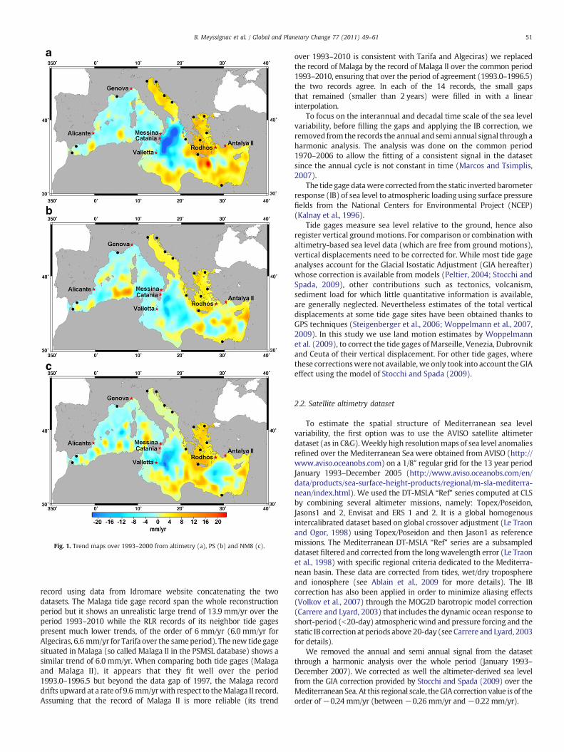
Fig. 1. Trend maps over 1993–2000 from altimetry (a), PS (b) and NM8 (c).

51B. Meyssignac et al. / Global and Planetary Change 77 (2011) 49–61

record using data from Idromare website concatenating the twodatasets. The Malaga tide gage record span the whole reconstructionperiod but it shows an unrealistic large trend of 13.9 mm/yr over theperiod 1993–2010 while the RLR records of its neighbor tide gagespresent much lower trends, of the order of 6 mm/yr (6.0 mm/yr forAlgeciras, 6.6 mm/yr for Tarifa over the sameperiod). The new tide gagesituated in Malaga (so called Malaga II in the PSMSL database) shows asimilar trend of 6.0 mm/yr. When comparing both tide gages (Malagaand Malaga II), it appears that they fit well over the period1993.0–1996.5 but beyond the data gap of 1997, the Malaga recorddrifts upward at a rate of 9.6 mm/yrwith respect to theMalaga II record.Assuming that the record of Malaga II is more reliable (its trend

over 1993–2010 is consistent with Tarifa and Algeciras) we replacedthe record of Malaga by the record of Malaga II over the common period1993–2010, ensuring that over the period of agreement (1993.0–1996.5)the two records agree. In each of the 14 records, the small gapsthat remained (smaller than 2 years) were filled in with a linearinterpolation.

To focus on the interannual and decadal time scale of the sea levelvariability, before filling the gaps and applying the IB correction, weremoved from the records the annual and semi annual signal through aharmonic analysis. The analysis was done on the common period1970–2006 to allow the fitting of a consistent signal in the datasetsince the annual cycle is not constant in time (Marcos and Tsimplis,2007).

The tide gage datawere corrected fromthe static inverted barometerresponse (IB) of sea level to atmospheric loading using surface pressurefields from the National Centers for Environmental Project (NCEP)(Kalnay et al., 1996).

Tide gages measure sea level relative to the ground, hence alsoregister vertical groundmotions. For comparison or combination withaltimetry-based sea level data (which are free from ground motions),vertical displacements need to be corrected for. While most tide gageanalyses account for the Glacial Isostatic Adjustment (GIA hereafter)whose correction is available from models (Peltier, 2004; Stocchi andSpada, 2009), other contributions such as tectonics, volcanism,sediment load for which little quantitative information is available,are generally neglected. Nevertheless estimates of the total verticaldisplacements at some tide gage sites have been obtained thanks toGPS techniques (Steigenberger et al., 2006; Woppelmann et al., 2007,2009). In this study we use land motion estimates by Woppelmannet al. (2009), to correct the tide gages of Marseille, Venezia, Dubrovnikand Ceuta of their vertical displacement. For other tide gages, wherethese correctionswere not available, we only took into account theGIAeffect using the model of Stocchi and Spada (2009).

2.2. Satellite altimetry dataset

To estimate the spatial structure of Mediterranean sea levelvariability, the first option was to use the AVISO satellite altimeterdataset (as in C&G).Weekly high resolutionmaps of sea level anomaliesrefined over the Mediterranean Sea were obtained from AVISO (http://www.aviso.oceanobs.com) on a 1/8° regular grid for the 13 year periodJanuary 1993–December 2005 (http://www.aviso.oceanobs.com/en/data/products/sea-surface-height-products/regional/m-sla-mediterra-nean/index.html). We used the DT-MSLA “Ref” series computed at CLSby combining several altimeter missions, namely: Topex/Poseidon,Jasons1 and 2, Envisat and ERS 1 and 2. It is a global homogenousintercalibrated dataset based on global crossover adjustment (Le Traonand Ogor, 1998) using Topex/Poseidon and then Jason1 as referencemissions. The Mediterranean DT-MSLA “Ref” series are a subsampleddataset filtered and corrected from the longwavelength error (Le Traonet al., 1998) with specific regional criteria dedicated to the Mediterra-nean basin. These data are corrected from tides, wet/dry troposphereand ionosphere (see Ablain et al., 2009 for more details). The IBcorrection has also been applied in order to minimize aliasing effects(Volkov et al., 2007) through the MOG2D barotropic model correction(Carrere and Lyard, 2003) that includes the dynamic ocean response toshort-period (b20-day) atmospheric wind and pressure forcing and thestatic IB correction at periods above 20-day (see Carrere and Lyard, 2003for details).

We removed the annual and semi annual signal from the datasetthrough a harmonic analysis over the whole period (January 1993–December 2007). We corrected as well the altimeter-derived sea levelfrom the GIA correction provided by Stocchi and Spada (2009) over theMediterranean Sea. At this regional scale, theGIA correction value is of theorder of−0.24 mm/yr (between−0.26 mm/yr and−0.22 mm/yr).

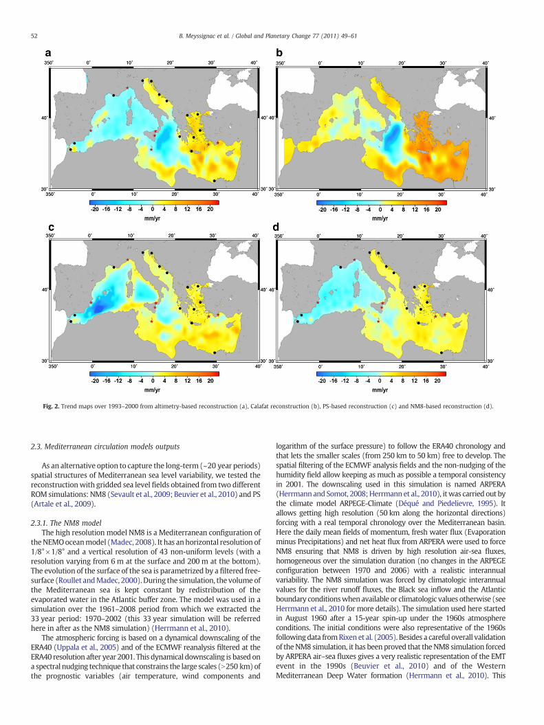
Fig. 2. Trend maps over 1993–2000 from altimetry-based reconstruction (a), Calafat reconstruction (b), PS-based reconstruction (c) and NM8-based reconstruction (d).

52 B. Meyssignac et al. / Global and Planetary Change 77 (2011) 49–61

2.3. Mediterranean circulation models outputs

As an alternative option to capture the long-term (~20 year periods)spatial structures of Mediterranean sea level variability, we tested thereconstructionwith gridded sea level fields obtained from two differentROM simulations: NM8 (Sevault et al., 2009; Beuvier et al., 2010) and PS(Artale et al., 2009).

2.3.1. The NM8 modelThe high resolution model NM8 is a Mediterranean configuration of

theNEMOoceanmodel (Madec, 2008). It has anhorizontal resolution of1/8°×1/8° and a vertical resolution of 43 non-uniform levels (with aresolution varying from 6 m at the surface and 200 m at the bottom).The evolution of the surface of the sea is parametrized by a filtered free-surface (Roullet andMadec, 2000).During the simulation, the volume ofthe Mediterranean sea is kept constant by redistribution of theevaporated water in the Atlantic buffer zone. The model was used in asimulation over the 1961–2008 period from which we extracted the33 year period: 1970–2002 (this 33 year simulation will be referredhere in after as the NM8 simulation) (Herrmann et al., 2010).

The atmospheric forcing is based on a dynamical downscaling of theERA40 (Uppala et al., 2005) and of the ECMWF reanalysis filtered at theERA40 resolution after year 2001. This dynamical downscaling is based ona spectral nudging technique that constrains the large scales (N250 km)ofthe prognostic variables (air temperature, wind components and

logarithm of the surface pressure) to follow the ERA40 chronology andthat lets the smaller scales (from 250 km to 50 km) free to develop. Thespatial filtering of the ECMWF analysis fields and the non-nudging of thehumidity field allow keeping as much as possible a temporal consistencyin 2001. The downscaling used in this simulation is named ARPERA(Herrmannand Somot, 2008;Herrmann et al., 2010), itwas carried out bythe climate model ARPEGE-Climate (Déqué and Piedelievre, 1995). Itallows getting high resolution (50 km along the horizontal directions)forcing with a real temporal chronology over the Mediterranean basin.Here the daily mean fields of momentum, fresh water flux (Evaporationminus Precipitations) and net heat flux from ARPERA were used to forceNM8 ensuring that NM8 is driven by high resolution air-sea fluxes,homogeneous over the simulation duration (no changes in the ARPEGEconfiguration between 1970 and 2006) with a realistic interannualvariability. The NM8 simulation was forced by climatologic interannualvalues for the river runoff fluxes, the Black sea inflow and the Atlanticboundary conditionswhenavailable or climatologic values otherwise (seeHerrmann et al., 2010 for more details). The simulation used here startedin August 1960 after a 15-year spin-up under the 1960s atmosphereconditions. The initial conditions were also representative of the 1960sfollowingdata fromRixen et al. (2005). Besides a careful overall validationof theNM8 simulation, it has been proved that theNM8 simulation forcedby ARPERA air–sea fluxes gives a very realistic representation of the EMTevent in the 1990s (Beuvier et al., 2010) and of the WesternMediterranean Deep Water formation (Herrmann et al., 2010). This

Fig. 3. Correlation maps over 1993–2000 between altimetry and our altimetry-based reconstruction (a), C&G reconstruction (b), PS-based reconstruction (c) and NM8-basedreconstruction (d).

53B. Meyssignac et al. / Global and Planetary Change 77 (2011) 49–61

version of NM8 includes the coding of the sea level including the absolutesteric sea level but excluding the pressure effect and the changes in theAtlantic Ocean sea level.

2.3.2. The PS modelThe PS model is an Atmosphere–Ocean regional climate model for

the Mediterranean basin. It is composed of the RegCM3 atmosphericregional model (Pal et al., 2007) and a Mediterranean configuration ofthe MITgcm ocean model (Artale et al., 2009) coupled through theOASIS3 coupler (Valcke and Redler, 2006). In the current study, we onlyuse the outputs of the ocean component of PS that is to say TheMITgcmmodel. It is a free-surface model with 1/8°×1/8° horizontal resolutionand 42non-uniformvertical levels (with a resolution varying from10 mat the surface and 300 m at the bottom). The volume of theMediterranean sea is kept constant during the 37 year simulation as inNM8 but since the freshwater forcing (Evaporationminus Precipitationminus river runoff) is applied as a virtual salt flux, here the net volumetransport through the Strait of Gibraltar is zero. Atmospheric forcing(wind stress, heatfluxes, evaporation and precipitation) is computed bythe RegCM3 (RegCM3 is a 3-dimensional, sigma coordinate hydrostaticregional climate model with a uniform horizontal resolution of 30 km).Only the river runoff fluxes are climatologic values computed apart(Struglia et al., 2004). The inflow from the Black sea is considered as anextra river flux. In this simulation the lateral boundary conditions aresuppliedby theERA40 reanalysis (Uppala et al., 2005)while theMITgcmcomponent provides the Sea Surface Temperature (SST) field.

ThePS run starts in1958andends in2002. For consistent comparisonswith the NM8 model, we extracted from this simulation the 33 yearsperiod 1970–2002.

Fromboth simulations, total sea level change is computed as the sumof circulation and steric components. The circulation sea level change isgiven by the surface deformation while the steric sea level change isdeduced at each grid point from the vertical integration of the specificvolume anomaly caused by temperature and salinity anomalies. Whencomputing global mean sea level from ocean reanalyses, it is classical toapply a basin-averaged, time-varying factor corresponding to theuniform steric effect (as explained by Greatbatch, 1994). However,here this correction is useless because we remove the total basin-average timevarying sea level from themodels (and the altimetrywhenit is used). Indeed we only use the spatial patterns of the sea level fromthe models (or the altimetry) to interpolate the tide gage records andreconstruct the past Mediterranean sea level. Moreover since we areonly interested in the interannual tomultidecadal sea level fluctuations,the annual and semi annual signalswere removed aswell from both sealevel fields through an harmonic analysis over thewhole period January1970–December 2002.

Fig. 1 shows the trends over 1993–2000 of the sea level computedfrom a) altimetry, b) the PS run and c) the NM8 run. The very goodagreement between the three maps confirms that the two ROM runsreproducewell theMediterranean sea level at least over the last decade.The signal in the ROM runs appears slightly smaller but the negativepatterns of theWestern and Ionian basin and the positive pattern of theAegean basin are consistent with the altimetry.

Fig. 4. Comparison of the altimetry reconstruction (a), Calafat reconstruction (b), PS-based reconstruction (c) and NM8-based reconstruction (d) with the tide gages of Alicante,Genova, Antalya II, Rodhos, Valletta, Catania and Messina (from top to bottom on the figure).

54 B. Meyssignac et al. / Global and Planetary Change 77 (2011) 49–61

3. Reconstruction methodology

Themethod used to reconstruct past (over 1970–2006) sea level in 2dimensions over the Mediterranean Basin is based on the reducedoptimal interpolation described by Kaplan et al. (2000) and used byChurch et al. (2004) and C&G to reconstruct past sea level. The ideaconsists in interpolating in 2-D the long tide gage records thanks to atime varying linear combination of the spatial patterns of a 2-D sea levelgrid (eitherAltimetryor ROMs). Thismethodhas 2 steps. In thefirst stepan EOF decomposition (Preisendorfer, 1988; Toumazou and Cretaux,2001) of a 2-D sea level grid (from altimetry or a Regional CirculationModel) is done. This decomposition allows to separate the spatiallywellresolved signal (here represented by a matrix H, with m lines for eachspatial point andn columns for each date) into spatialmodes (EOFs) andtheir related temporal amplitude as follow:

H x; y; tð Þ = U x; yð Þα tð Þ: ð1Þ

In this equation U(x,y) stands for the spatial modes and α(t) fortheir amplitude. Assuming that the spatial modes U(x,y) arestationary in time (see the discussion below), we deduce that thereconstructed sea level field of the Mediterranean basin over the longperiod 1970–2006 (called hereHR(x,y, t)) has an Empirical OrthogonalDecomposition as follow:

HR x; y; tð Þ = U x; yð ÞαR tð Þ

where αR(t) represents the new amplitudes of the EOFs over 1970–2006.

The second step consists of computing the new amplitudes overthewhole period 1970–2006 thanks to the tide gage records. It is donethrough a least square optimal procedure that minimizes thedifference between the reconstructed field and the tide gage recordsat the tide gage locations.

In the first step, the EOFmodes and amplitudes of the 2-D sea levelgrids are computed through a singular value decomposition approach,such that:

H = USVt ð2Þ

whereU(x,y) still stands for theEOF spatialmodes, S is a diagonalmatrixcontaining the singular values of Hand Vrepresents the temporal eigenmodes. At this stage the amplitude of the EOF modes can be simplywritten as α(t)=SVT. Conceptually, each EOF k (kth column of U(x,y)multiplied by the kth line of α(t):Uk(x,y).αk(t)) is a spatio-temporalpattern of sea level variability that accounts for a percentage of the totalvariance of the sea level signal.

The low-order EOFs (eigenvectors of the largest singular values)explain most of the variance and contain the largest spatial scales of thesignal. The higher-order EOFs contain smaller spatial scale patterns andare increasingly affected by noise. Besides, their amplitude is decreas-ingly well resolved by the least squares procedure because thesparseness of the set of in situ gages does not allow resolving toosmall scale patterns. For efficiency, the reconstruction over theMediterranean basin uses a subset of the Mlowest-order EOFs (thebest fit between maximum variance explained and minimum noiseperturbation led us to choose M=3, which account for at least 69% of

Table 1Correlation and trend's differences between the independent tide gage records (indicated by stars on the maps and shown in Fig. 1) and the corresponding reconstructed time series.Correlations and trend differences are computed over 2 different periods: until 2001 to be able to compare themwith the reconstruction of Calafat and Gomis and until 2006 to have thecorrelations over the whole reconstructed time span. All the correlations computed have a significance level higher than 99% (except for the correlation between the C&G reconstructionand the Messina record).

Name ofthe tidegage

Calafat and Gomisreconstruction

Altimetry-based reconstruction PS-based reconstruction NM8-based reconstruction

Corr→2001

Trenddiff→2006

Correlation Trend difference in mm/yr Correlation Trend difference in mm/yr Correlation Trend difference in mm/yr

→2001 →2006 → 2001 → 2006 →2001 →2006 → 2001 → 2006 →2001 →2006 → 2001 → 2006

Alicante 0.67 −0.3±0.4 0.59 0.59 −0.1±0.4 −0.1±0.4 0.44 0.44 0.0±0.7 −0.1±0.7 0.50 0.50 1.9±0.5 1.9±0.5Genova 0.54 −1.8±1.0 0.49 0.49 0.2±1.1 0.2±1.1 0.42 0.41 −3.4±1.1 −3.4±1.1 0.59 0.59 −1.1±1.0 −1.1±1.0Antalya II 0.48 1.8±2.3 0.43 0.46 −1.6±2.3 −2.2±2.1 0.47 0.51 −2.5±2.0 −3.0±1.8 0.46 0.50 −2.6±2.1 −3.1±1.8Rodhos 0.39 1.07±0.9 0.57 0.55 0.3±0.7 0.0±0.6 0.55 0.54 1.6±0.7 1.1±0.6 0.56 0.55 1.3±0.7 0.8±0.5Valletta 0.45 −2.8±2.1 0.25 0.27 −3.8±2.5 −2.1±1.4 0.36 0.40 2.9±2.6 0.2±1.5 0.32 0.39 0.7±2.8 −0.5±1.6Catania 0.54 −6.9±4.9 0.51 0.51 3.2±6.6 3.2±6.6 0.67 0.67 0.2±4.7 0.1±4.7 0.69 0.69 −0.4±4.2 −0.4±4.2Messina −0.08 −27.4±6.6 0.10 0.16 −23.6±6.8 −12.4±3.7 0.30 0.28 −17.5±6.8 −11.7±3.6 0.31 0.32 −18.1±6.7 −11.0±3.6

55B. Meyssignac et al. / Global and Planetary Change 77 (2011) 49–61

the total variance of the sea level grid data). Consequently, the datamatrix H can be written as:

HM = UM x; yð Þ:α tð Þ

where α(t)=SMVMT is the matrix of the amplitude of theMlowest EOFs.

Following Kaplan et al. (2000), in the second step, we compute, at eachtime step over the time span of the in situ records, the amplitudes byminimizing the cost function:

S αð Þ = PUMα−H0� �T

R−1 PUMα−H0� �

+ αTΛ−1α ð3Þ

In S(α),H0 is the sea level observed by the tide gages, Pis a projectionmatrix equal to 1 when and where in situ records are available and0 otherwise and Λ is a diagonal matrix of the largest eigenvalues of thecovariance matrix. R is the error covariance matrix accounting for thedata error covariance matrix (instrumental error) and the error due tothe truncation of the set of EOFs to only the first M EOFs. The secondterm on the right hand side of the function is a constraint on the EOFspectrum of the solution. It prevents the least squares procedure to becontaminated by high-frequency noise (it filters out non significantsolutions that display too much variance at grid points without nearbyobservations). The least squares procedure is then applied to the virtualin situ tide gage records (H0). It provides the reconstructed amplitudeαR of the EOFs.

Since tide gage records are all relative to their own local datum thatare not cross-referenced over the basin, this solutionmay bepolluted byspatial variability of the in situ tide gage records reference surface notnecessarily consistent with the altimetry reference surface or the ROMreference surface. To copewith this problem, we have solved Eq. (3) forchanges in sea level between adjacent steps following Church et al.(2004). Once changes in amplitude have been obtained at each timestep, the amplitudes themselves have been recovered, integratingbackward in time. The integration constants are chosen to equal thereconstructed EOF amplitudes mean to the 2-D gridded sea level EOFamplitude mean over the 2-D gridded sea level field period, ensuringconsistency between both sets of EOFs.

Another issue with sea level reconstruction in the Mediterraneanbasin is the strong basin-average signal of theMediterranean basin. Thissignal, that is contained in the tide gages, is hardly captured by the fewEOFs we use. The reason is that before the computation of the EOFs, foreach gridded times series (the 2 ROMs and the altimetry) we haveremoved the basin-averaged time varying sea level (see Section 2) sothe set of EOFs we use is not adapted to reconstruct any basin averagesea level. Hence, as in Church et al. (2004), we added in the set of EOFs aspatially uniform EOF (so called EOF0 in Church et al., 2004 and in C&G)to capture, from the tide gages, the basin-averaged signal of theMediterranean in the past. An advantage of this procedure is that itavoids pouring the strong basin-average sea level signal in different

EOFs. Note that tests carried out with and without the EOF0 resulted inalmost the same reconstructions.

Finally the reconstructed field of sea level is obtained bymultiplyingthe first three EOFs plus the EOF0 with their reconstructed amplitude:

HR = UM x; yð Þ⋅αR tð Þ ð4Þ

At this point, the correction for the atmospheric effects of the tidegage dataset and the altimetry dataset appears particularly importantbecause of the sparsely distribution of the tide gage data set. Indeed,changes over time in atmospheric pressure patterns can be mis-represented with such a sparse network of tide gages biased towardthe north of the Mediterranean basin. For example if atmosphericpressure patterns had a bias toward the north in the past this wouldbe misinterpreted as a change in past global Mediterranean sea levelalthough it is not the case. As discussed above, beyond 20-day periods,the correction applied to account for the ocean response toatmospheric forcing is the static IB (1 mbar corresponds to 1 cm sealevel). It is known that in the Mediterranean Sea, there is a slight low-frequency non static component. However this effect remains small(a few% of the static part) and for the purpose of the present study canbe neglected (F. Lyard, personal communication).

4. Reconstructed sea level

4.1. Validation over the altimetry period

Afirstway to check the validity of the reconstructions is to look at thereconstructed sea level over the altimetry period and check that thereconstructed spatial trend patterns and variability are similar to theobserved one by the altimetry. Fig. 2 shows the spatial trend maps(uniform trend removed) over 1993–2000 (because the C&G recon-struction ends inDecember 2000) of the altimetry-based reconstruction(Fig. 2a), the C&G reconstruction (see Fig. 2b) and from the twoROM-based reconstructions (Fig. 2c and d). For this comparison, theC&G reconstructionwas a posteriori corrected for the IB effect. This wasdone by simply removing at each time step, NCEP IB grids to the C&Greconstructed sea level.

We note a good agreement between the spatial trend patterns of thereconstructed maps and satellite altimetry presented in Fig. 1a. Ouraltimetry reconstruction and the C&G reconstruction are very close toeach other and they are very consistent with the satellite altimetrysignal (Fig. 1a) as expected. The only difference that can benoticed is thelower negative pattern in the Ionian Sea in our altimetry reconstruction.To a lesser extent, the two ROM-based reconstructed trend patterns areconsistent as well with the satellite altimetry patterns in each basin butthey show a lower negative pattern in the Ionian Sea and a lowerpositive pattern in the Aegean Sea.

Fig. 5. EOF decomposition over 1970–2006 of the reconstructions. a) and b) show the modes 1 and 2 of the altimetry-based reconstruction. c) and d) show the modes 1 and 2 of thePS-based reconstruction and e) and f) show the modes 1 and 2 of the NM8-based reconstruction. The temporal curves have been smoothed with a 12-month running mean.

56 B. Meyssignac et al. / Global and Planetary Change 77 (2011) 49–61

57B. Meyssignac et al. / Global and Planetary Change 77 (2011) 49–61

We compare as well the reconstructed sea level variability with theobserved one over the same period 1993–2000. To do so, we computed,at each grid point, the correlation between the reconstructed time seriesand the observed altimetry time series over the period 1993–2000. Theresults are presented in Fig. 3. All reconstructions present positivesignificant correlations in the central and easternMediterranean basins.Correlations are less good in the western basin. C&G reconstruction(Fig. 3b) shows particularly good correlations in the Ionian basin whileour altimetry-based reconstruction (Fig. 3a) performs less in this region.This is probably due to the fact that C&G used the tide gage of Vallettaover 1989–2000 to do their reconstruction: it must have constrainedbetter their reconstructed variability in this region. Nevertheless ouraltimetry-based reconstruction seems to perform slightly better in thewestern basin. It is probably linked to the choice of the tide gages in thisregion as well. The reconstruction that performs the best in terms ofreproduced variability over 1993–2000 appears to be the NM8-basedreconstruction (Fig. 3d). The geographically averaged correlations foreach case amount to0.46 for our altimetry based reconstruction, 0.49 forthe C&G reconstruction, 0.44 for the PS-based reconstruction and 0.50for the NM8-based reconstruction. This clearly shows the ability of themodel-based reconstructions (especially the NM8-based reconstruc-tion) to reproduce reliably the past sea level variability.

4.2. Validation with tide gage records

Another way to validate the reconstructions over the whole period1970–2006 is to compare the reconstructed sea level fields with tidegage records that were not taken into account in the reconstructionprocess.

Note that the coastal tide gage records we use are monthly averagesand contain potential contributions from regional or local coastalprocesses (e.g. local variability of narrow shelf currents,flooding events,wind-forced coastal waves, etc.) aswell as landmotion unrelated to thesignal we are attempting to reconstruct here. Moreover, with thereconstructed sea level fields, the optimal interpolation method usesonly part of the total sea level grids variance to reconstruct the total sealevel. Consequently, we expect to reconstruct only part of the totalobserved variance of the tide gage records but it should be represen-tative of the reconstruction validity.

Fig. 4 shows the comparison of the reconstructed fields with 7 tidegage records that were not used in our reconstruction. These are theAlicante and Genova records in thewestern basin (data from the PSMSLdatabase), the Valletta, Catania and Messina records in the Ionian Sea(data from the Italian tide gage network (www.idromare.it)) and theRodhos and the Antalya II records in the eastern basin (data fromPSMSL). Location of the tide gages is indicated in Fig. 1 (black stars). Foreach record, we applied the same corrections as explained earlier inSection 2.1: the annual and semi annual signals were removed, and IBand GIA corrections were applied. In Fig. 4, observed tide gage recordsare plotted in red and reconstructions at the gages location are in black.Table 1 sum up the correlation and the trend differences computed onthe basis of this figure. Fig. 4 and Table 1 illustrate the strengths andweaknesses of each of the reconstructions (and of the tide gage recordsas well):

• In thewesternMediterranean, 2 long RLR records from PSMSL, Alicanteand Genova, are available to check the reconstructions. Their variabilityis fairly well reproduced (correlation ~0.5) by both altimetryreconstructions (C&G reconstruction and our reconstruction) (Fig. 4aand b and Table 1 columns 2 and 4). Alicante record variability isexceptionally well reproduced (correlation of 0.67) by the C&Greconstruction certainly because this record is used in their reconstruc-tion process. The trends appear consistent with each other except atGenova for the C&G reconstruction that underestimates its trend by1.8 mm/yr. Looking at the ROM and our altimetry reconstruction overthewhole period (until 2006) (Fig. 4b, c and d and Table 1 columns 5, 9

and 13) the NM8 reconstruction appears to perform better in term ofinterannual variability.

• The variability at Antalya II is quite well reproduced by both altimetryreconstructions with a similar correlation of ~0.45 (Fig. 4a and b andTable 1 columns 2 and 4) but the C&G reconstruction shows asignificantly lower correlation for the Rodhos record (correlation of0.39) than ours (correlation of 0.57). The model reconstructions(Fig. 4c and d and Table 1 columns 9 and 13) appear homogenous overthe Levantine basin with correlations of ~0.5 with both tide gagerecords (as for the altimetry reconstruction) (Fig. 4a and Table 1column 5).

• In the Ionian basin, unfortunately we could not find long records tocheck the reconstructions. The longest available record is the RLRrecord of Valletta from PSMSL over 1989–2006. Two additionalrecords could be found in the Ionian basin, the Catania and Messinarecord from the Idromare database (www.idromare.it). These areactually too short to give a reliable verification of the reconstructedtrend but they give interesting insights on the interannual variabilityof the Ionian sea level. TheMessina record was selected because of itsinteresting location. However, it should be taken with caution since itshows many suspicious jumps (in particular in 1998) as previouslynoticed by Fenoglio-Marc et al. (2004). The two altimetry reconstruc-tions (Fig. 4a and b and Table 1 columns 2 and 4) show very similarcorrelations with the tide gage records except for the Valletta recordthat shows higher correlation with the C&G reconstruction (probablybecause this record was used in the C&G reconstruction). Over1970–2006, the model reconstructions show consistent, and highercorrelations at all tide gages in the Ionian basin than the altimetryreconstruction (Fig. 4a, c and d and column 5, 9 and 13 of Table 1).They show an exceptionally high correlation of 0.68 with the Cataniarecord.As for the trendof theValletta record it is actuallywell resolvedonly by the ROM reconstructions while it is strongly underestimatedby the altimetry reconstruction (column 6, 10 and 14 of Table 1).

4.3. Mediterranean sea level variability

In Fig. 5, we present, the 2-D reconstructed fields based on thealtimetry dataset, the PS and the NM8 runs respectively. We haveperformed an EOF decomposition over the whole reconstructed timespan 1970–2006 for the three fields. Only the first 2 modes (EOF1 andEOF2) are presented because they account for the largest percentage ofthe total variance of the signal. The temporal curves have beensmoothed with a 12-month running mean in order to emphasize theinterannual variability. EOFmodes 1 of eachof the three reconstructions(Fig. 5a, c and e) – 39, 78 and 24% of total variance respectively – showno trend and amaximum in 1990 in its temporal amplitude. EOFmodes2 (31, 5 and19%of total variance respectively, see Fig. 5b, d and f) exhibithigh and low frequency signal (period ~15 years) over 1970–2006. TheEOF spatial patterns differ from one reconstruction to another. We notestrong similarities between EOFmode1 patterns of each reconstruction,with a global dipole marked by a positive pattern in the Western basinand a negative pattern in the Levantine basin.Nevertheless they differ inthe Ionian Sea: the NM8 reconstruction shows a negative patternwhereas the altimetry reconstruction shows a positive one and the PSreconstruction a pattern somehow between the both. Concerning theEOF mode 2 patterns, the three reconstructions are fairly consistent inthe Ionian and Levantine basin with a strong positive anomaly in theIonian and Levantine Sea and negative one in the Agean Sea. In thewestern basin, the altimetry-based and the PS-based reconstructionsagree well, with a dipole positive in the eastern part while the NM8-based reconstruction patterns are inversed there. In Fig. 6, thereconstructed basin-average sea level (i.e., the EOF0 of each recon-struction) is shown and compared to the satellite altimetry sea levelover 1993–2006. As for the EOFs, it has been smoothed by a 12-monthrunning mean to emphasize the interannual to decadal variability. Thefour reconstructed sea level curves show the same decadal variability.

Fig. 6. Basin-average sea level from Satellite altimetry (black dashed line), our altimetry-based reconstruction (blue plain line), the C&G reconstruction (cyan plain line), the PS-basedreconstruction (green plain line) and the NM8-based reconstruction (red plain line). The temporal curves have been smoothed with a 12-month running mean.

58 B. Meyssignac et al. / Global and Planetary Change 77 (2011) 49–61

Their interannual variability is very similar as well over the periods1970–1985 and 1994–2006. But somedifferences appear between 1985and 1995: the PS-based reconstructed basin average sea level shows ahigh level that does not appear in the other reconstructions. Over thealtimetry era, all reconstructions show a mean sea level similar to theobserved, altimetry-based global mean sea level. In Fig.6, the gray zonerepresents the uncertainty in the NM8-based reconstructed mean sealevel. This uncertainty is based on the sum of errors due to the least-squares inversion (as presented in Section 3) and errors of the in siturecords. This latter error is estimated from a bootstrap method (Efronand Tibshirani, 1993) for standard errors of the in situ water levels foreach month (significant at the 95% level).

5. Discussion

The altimetry-based reconstruction developed in this study has beencompared with the C&G one over the period 1970–2000 only, becausethe C&G reconstruction stops in December 2000. We note very similarcorrelations between the two altimetry-based reconstructions and thetide gage records (Table 1, columns 1 and 3). It suggests that the twoaltimetry reconstructions are consistent and that the techniques used inC&G and the present study, end up with very close results. This meansthat removing IB before the reconstruction (this study) or after has littleimpact on the results.

The Valletta record cannot actually be considered as an independentreference to compare with the two altimetry reconstructions since it isused in C&G reconstruction (between 1995 and 2000) and not in theother (by using only tide gage records that spanned the whole period1970–2006 and excluding others like Valletta, we ensured thereconstruction to be homogenous over the whole time span). As forthe Rhodos record it is not clear why it shows higher correlation withour altimetry reconstruction. An explanation could be that ourreconstruction is more constrained in the Levantine basin thanks tothe use of the Alexandria record. But this remains to be confirmed.

Considering the reconstructed variability of the basin-averagedMediterranean sea level, the consistency of the two altimetryreconstructions, while the tide gage dataset differ, gives confidence inthe robustness of the results presented by C&G and in this study.However, the spatial trend maps do not match as well (see Fig. 7). Thetwomethods lead to the samebasin-averaged trend of ~1.1 mm/yr over1970–2000 (1.0 mm/yr and 1.2 mm/yr for C&G and this studyrespectively) but differ in the trend patterns. The two reconstructionsshow the same geometry in the trend patterns (positive pattern in theIonian Sea and in the Tyrrhenian Sea) but the C&G reconstructionexhibits lower variability. The comparison of the reconstructions withindependent long tide gage record (Table 1) tend to show that in the

western basin the trends of our altimetry-based reconstruction arecloser to the trends observed at tide gages (see columns 3 and 6 ofTable 1 for the Alicante and the Genova records). In the eastern basin,the C&G reconstruction tend to overestimate the trends by ~1 mm/yrwhile our altimetry reconstruction tend to underestimate the trend atAntalya, as shown by the comparison with the Antalya and the Rodhostide gage trends. In the Ionian basin the tide gage trends used for thevalidation are not reliable because of too short records. Bothreconstructions seem to underestimate the trend at Valletta, but wecannot extrapolate for the rest of the Ionian Sea.

The three reconstructions presented here (altimetry and ROMbased) have been computed by the same process (same tide gagedataset). They only differ by the initial sea level grids used to estimatethe spatial variability statistics of theMediterranean sea level. Looking atthe correlations (Table 1, columns 5, 9 and 13) we note a goodconsistency of the three reconstructed sea level fields: the correlationsof each reconstructionwith independent tide gages never differ bymorethan 0.2 from one another. Looking more carefully, both modelreconstructions appear particularly consistent since their correlationswith tide gages do not differ by more than 0.06, except for the Genovarecord which has a surprising very low correlation with the PSreconstruction. Hence the two models give similar reconstructedinterannual variability. This point gives confidence in the robustnessof the model-based reconstruction process. Among the threereconstructions, even if they show similar results, the NM8 reconstruc-tion shows the highest correlations with the test tide gages.

At sub-basin scale, the conclusion is less clear. Some discrepanciesappear among the reconstructions. While in the eastern basin, thethree reconstructions have similar correlations with the test tidegages, in the western basin, the NM8 and the altimetry reconstructionshow higher correlation (see columns 5, 9 and 13 of Table 1 for theAntalya and Rodhos records).

It is in the Ionian Sea where the highest discrepancies can be seen:bothmodel reconstructions showsignificanthigher correlationwith thetest tide gages of Valletta, Catania and Messina than the altimetryreconstruction. As said earlier, the Ionian basin waters have beenstrongly impacted by the EMT. This event impacted the Mediterraneancirculation during the 1990s until now (Roether et al., 2007) and seemsto be responsible for a change in surface circulation, from anti-cyclonicto cyclonic in the Ionian basin in 1998 (Vera et al., 2009). This change incirculation is characterized by the very strong negative pattern in theIonian Sea that can be seen in the trend maps of the models and thealtimetry over the period 1993–2000 (see Fig. 2) (Vera et al., 2009). Thisexceptional signal dominates the altimetry EOFs since the altimetrydataset only cover the EMT-period (i.e. since 1993). It is less strong inboth model-based reconstructions because they capture a long term

Fig. 7. Map of sea level trends over 1970–2006 of a) the altimetry reconstruction., b) the C&G reconstruction, c) the PS reconstruction and d) the NM8 reconstruction. For each mapwe have removed the basin-averaged sea level trend computed over 1970–2006which is of 1.2 mm/yr for the altimetry reconstruction, 1.0 for the C&G reconstruction, 0.8 mm/yr forthe PS reconstruction and 1.4 mm/yr for the NM8 reconstruction.

59B. Meyssignac et al. / Global and Planetary Change 77 (2011) 49–61

signal not dominated by the EMT event. This could explain thedifference of correlations between the reconstructions in the Ionianbasin. Looking at Fig. 4a, c and d, the model-based reconstructionsappear indeed to better reconstruct the signal prior to the 1990s for theValletta record for example.

In terms of trends over the period 1970–2000, the three re-constructions of this study plus C&G present strong discrepancies.Only the ROM reconstructions appear to properly reconstruct theValletta record trend (Table 1 column 15). In the western basin thealtimetry-based reconstruction (of this study) is the only one that seemsto reproduce both the Genova and Alicante trends. In the eastern basinthe trends of Rodhos and Antalya II are not captured by anyreconstruction despite their proximity. This point highlights thesensitivity of this region.

The NM8 reconstruction shows better interannual to decadalreconstructed variability so itwas used as the reference reconstructionto investigate the potential past influence of some forcingmodes of thecoupled Atmosphere–Ocean system on the Mediterranean sea level.Fig. 8 compares the amplitude of EOF1 and of the negative EOF2 of theNM8 reconstructionwith the North Atlantic Oscillation –NAO – index.For the NAO index we used the monthly index from the ClimateAnalysis Section NCAR at Boulder, USA (Hurrell, 1995) based on thedifference of normalized sea level pressure between Ponta Delgada(Azores) and Reykjavik (Iceland). The NAO index was smoothed by a12-month running mean and compared to the EOFs of the NM8

reconstruction (smoothed as well by the 12-month running mean). Itturns out that before ~1993.5 (date indicated by a gray bar in Fig. 8),the EOF1 temporal curve of the NM8 reconstruction shows acorrelation with the NAO index of up to 0.60 (with a significancelevel N0.99) while over the period 1993.5–2006 the correlation getsdown to −0.37. On the other hand, after ~1993.5 the negative EOF2temporal curve of the NM8 reconstruction shows a high correlationwith NAO index of 0.54 (with a SL N0.99) while over the period1970–1993.5 it only amounts to−0.30. It is interesting to note that thecorrelation with NAO switches from EOF1 to EOF2 at the epoch of theEMT occurrence.

6. Conclusions

Concerning the interannual/decadal variability of the Mediterra-nean sea level, the overall agreement of the reconstructions with eachother and with the test tide gage records gives confidence in thereconstructed sea level fields. The comparison of model-basedreconstructions and altimetry-based reconstructions confirms thisrobustness since they agree on global scale. At sub-basin scale, theROM-based reconstructions (especially the NM8-based reconstruc-tion) perform better in the Ionian basin than altimetry-based, and thisis probably due to a too strong representation of the EMT event in thealtimetry EOFs. This point highlights the advantage of using long ROM

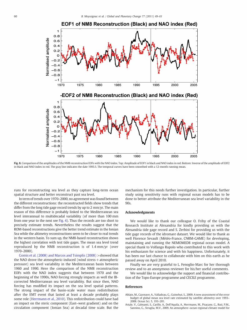
Fig. 8. Comparison of the amplitudes of theNM8 reconstruction EOFswith theNAO index. Top: Amplitude of EOF1 in black andNAO index in red. Bottom: Inverse of the amplitude of EOF2in black and NAO index in red. The gray line indicates the date 1993.5. The temporal curves have been smoothed with a 12-month running mean.

60 B. Meyssignac et al. / Global and Planetary Change 77 (2011) 49–61

runs for reconstructing sea level as they capture long-term oceanspatial structure and better reconstruct past sea level.

In termof trends over 1970–2000, no agreementwas foundbetweenthe different reconstructions: the reconstructed fields show trends thatdiffer from the long tide gage record trends by up to 2 mm/yr. Themainreason of this difference is probably linked to the Mediterranean sealevel interannual to multidecadal variability (of more than 100 mmfrom one year to the next see Fig. 4). Thus the records are too short toprecisely estimate trends. Nevertheless the results suggest that theROM-based reconstructions give the better trend estimate in the IonianSea while the altimetry reconstructions seem to be closer to real trendsin the western basin. To sum up, the NM8-based reconstruction showsthe highest correlation with test tide gages. The mean sea level trendreproduced by the NM8 reconstruction is of 1.4 mm/yr (over1970–2000).

Gomis et al. (2008) andMarcos and Tsimplis (2008) >showed thatthe NAO drove the atmospheric-induced (wind stress+atmosphericpressure) sea level variability in the Mediterranean basin between1960 and 1990. Here the comparison of the NM8 reconstructionEOFs with the NAO index suggests that between 1970 and thebeginning of the 1990s, NAO forcing strongly impacts as well the IB-corrected Mediterranean sea level variability. But since then, NAOforcing has modified its impact on the sea level spatial patterns.The strong impact of the basin-scale water mass redistributionafter the EMT event that lasted at least a decade probably playssome role (Herrmann et al., 2010). This redistribution could have hadan impact on the steric component (East–west gradient) and on thecirculation component (Ionian Sea) at decadal time scale. But the

mechanism for this needs further investigation. In particular, furtherstudy using sensitivity runs with regional ocean models has to bedone to better attribute the Mediterranean sea level variability in the90s.

Acknowledgments

We would like to thank our colleague O. Frihy of the CoastalResearch Institute at Alexandria for kindly providing us with theAlexandria tide gage record and S. Zerbini for providing us with thetide gage records of the idromare dataset. We would like to thank aswell Florence Sevault (Météo-France, CNRM-GAME) for developing,maintaining and running the NEMOMED8 regional ocean model. Aspecial thank to Volfango Rupolo who contributed to this work withhis enthusiasm for science and with his happiness. Unfortunately, ithas been our last chance to collaborate with him on this earth as hepassed away on April 2010.

Finally we are very grateful to L. Fenoglio-Marc for her thoroughreview and to an anonymous reviewer for his/her useful comments.

We would like to acknowledge the support and financial contribu-tion of the Topo-Europe programme and CECILE programme.

References

Ablain, M., Cazenave, A., Valladeau, G., Guinehut, S., 2009. A new assessment of the errorbudget of global mean sea level rate estimated by satellite altimetry over 1993–2008. Ocean Sci. 5, 193–201.

Artale, V., Calmanti, S., Carillo, A., Dell'Aquila, A., Herrmann, M., Pisacane, G., Ruti, P.M.,Sannino, G., Struglia, M.V., 2009. An atmosphere–ocean regional climate model for

61B. Meyssignac et al. / Global and Planetary Change 77 (2011) 49–61

the Mediterranean area: assessment of a present climate simulation. OceanModelling 30, 56–72.

Becker, M., Karpytchev, M., Davy, M., Doekes, K., 2009. Impact of a shift in mean on thesea level rise: application to the tide gauges in the Southern Netherlands.Continental Shelf Res. 29, 741–749.

Beuvier, J., Sevault, F., Herrmann, M., Kontoyiannis, H., Ludwig, W., Rixen, M., Stanev, E.,Beranger, K., Somot, S., 2010. Modelling the Mediterranean Sea interannualvariability during 1961–2000: focus on the Eastern Mediterranean Transient(EMT). J. Geophys Res. 115, C08017. doi:10.1029/2009JC005850.

Bindoff, N.L., Willebrand, J., Artale, V., Cazenave, A., Gregory, J.M., Gulev, S., Hanawa, K., LeQuéré, C., Levitus, S., Nojiri, Y., Shum, C.K., Talley, L.D., Unnikrishnan, A.S., 2007.Observations: oceanic climate change and sea level. Climate Change 2007:The Physical Science Basis. Cambridge University Press, pp. 385–432.

Cabanes, C., Cazenave, A., Le Provost, C., 2001. Sea level change from Topex-Poseidonaltimetry for 1993–999 and possible warming of the southern oceans. Geophys.Res. Lett. 28, 9–12.

Calafat, F.M., Gomis, D., 2009. Reconstruction of Mediterranean sea level fields for theperiod 1945–2000. Glob. Planet. Change 66, 225–234.

Carrere, L., Lyard, F., 2003. Modeling the barotropic response of the global ocean toatmospheric wind and pressure forcing — comparisons with observations.Geophys. Res. Lett. 6, 1275. doi:10.1029/2002GL016473.

Church, J.A., White, N.J., Coleman, R., Lambeck, K., Mitrovica, J.X., 2004. Estimates of theregional distribution of sea level rise over the 1950–2000 period. J. Clim. 17,2609–2625.

Déqué, M., Piedelievre, J.P., 1995. High-resolution climate simulation over Europe. Clim.Dyn. 11, 321–339.

Efron, B., Tibshirani, R.J., 1993. An Introduction to the Bootstrap. Chapman & Hall.Fenoglio-Marc, L., Groten, E., Dietz, C., 2004. Vertical land motion in the Mediterranean

sea from altimetry and tide gauge stations. Marine Geodey 27, 683–701.Frihy, O.E., Deabes, E.A., Shereet, S.M., Abdalla, F.A., 2010. Alexandria-Nile Delta coast,

Egypt: update and future projection of relative sea-level rise. Earth EnvironmentScience 2, 253–273. doi:10.1007/s12665-009-0340-x.

Gomis, D., Ruiz, S., Sotillo, M.G., Alvarez-Fanjul, E., Terradas, J., 2008. Low frequencyMediterranean sea level variability: the contribution of atmospheric pressure andwind. Glob. Planet. Change 63, 215–229.

Greatbatch, R.J., 1994. A note on the representation of steric sea-level in models thatconserve volume rather than mass. J. Geophys. Res. 99, 12767–12771.

Herrmann, M.J., Somot, S., 2008. Relevance of ERA40 dynamical downscaling formodeling deep convection in the Mediterranean Sea. Geophys. Res. Lett. 35,L04607. doi:10.1029/2007GL032442.

Herrmann, M., Sevault, F., Beuvier, J., Somot, S., 2010. What induced the exceptional2005 convection event in the northwestern Mediterranean basin? Answers from amodeling study. J. Geophys. Res. 115, C12051. doi:10.1029/2010JC006162.

Hurrell, J.W., 1995. Decadal trends in the North Atlantic Oscillation — regionaltemperatures and precipitations. Science 269, 676–679.

Josey, S.A., 2003. Changes in the heat and freshwater forcing of the easternMediterraneanand their influence on deep water formation. J. Geophys. Res. 108, 3237–3255.doi:10.1029/2003JC001778.

Kalnay, E., Kanamitsu, M., Kistler, R., Collins, W., Deaven, D., Gandin, L., Iredell, M., Saha, S.,White, G.,Woollen, J., Zhu, Y., Chelliah,M., Ebisuzaki,W., Higgins,W., Janowiak, J., Mo,K.C., Ropelewski, C., Wang, J., Leetmaa, A., Reynolds, R., Jenne, R., Joseph, D., 1996. TheNCEP/NCAR 40-year reanalysis project. Bull. Amer. Meteor. Soc. 77, 437–471.

Kaplan, A., Kushnir, Y., Cane, M.A., 2000. Reduced space optimal interpolation ofhistorical marine sea level pressure: 1854–1992. J. Clim. 13, 2987–3002.

Klein, B., Roether, W., Manca, B.B., Bregant, D., Beitzel, V., Kovacevic, V., Luchetta, A., 1999.The large deep water transient in the Eastern Mediterranean. Deep Sea Res. I. 46,371–414.

Lascaratos, A., Roether, W., Nittis, K., Klein, B., 1999. Recent changes in deep waterformation and spreading in the eastern Mediterranean Sea: a review. Progress inOceanography 44, 5–36.

Le Traon, P.Y., Nadal, F., Ducet, N., 1998. An improved mapping method of multisatellitealtimeter data. J. atmospheric oceanic technology 15, 522–534.

Le Traon, P.Y., Ogor, F., 1998. ERS-1/2 orbit improvement using TOPEX/POSEIDON: the2 cm challenge. J. Geophys. Res. 103, 8045–8057.

Llovel, W., Cazenave, A., Rogel, P., Lombard, A., Nguyen, M.B., 2009. Two-dimensionalreconstruction of past sea level (1950–2003) from tide gauge data and an OceanGeneral Circulation Model. Climate of the Past 5, 217–227.

Lombard, A., Cazenave, A., DoMinh, K., Cabanes, C., Nerem, R.S., 2005. Thermosteric sealevel rise for the past 50 years; comparisonwith tide gauges and inference onwatermass contribution. Glob. Planet. Change 4, 303–312.

Madec, G., 2008. Nemo ocean engine. Note du pôle modélisation no. 27. IPSL France.ISSN n°1288–1619.

Malanotte-Rizzoli, P., Manca, B.B., d'Alcala, M.R., Theocharis, A., Brenner, S., Budillon, G.,Ozsoy, E., 1999. The EasternMediterranean in the 80s and in the90s: the big transitionin the intermediate and deep circulations. Dynamics of Atmospheres and Oceans 29,365–395.

Marcos, M., Tsimplis, M.N., 2007. Variations of the seasonal sea level cycle in southernEurope. J. Geophys. Res. 112, C12011. doi:10.1029/2006JC004049.

Marcos, M., Tsimplis, M.N., 2008. Coastal sea level trends in southern Europe. Int. J.Geophys. 175, 70–82.

Milne, G.A., Gehrels, W.R., Hughes, C.W., Tamisiea, M.E., 2009. Identifying the causes ofsea-level change. Nature Geoscience 2, 471–478.

Pal, J.S., Giorgi, F., Bi, X.Q., Elguindi, N., Solmon, F., Gao, X.J., Rauscher, S.A., Francisco, R.,Zakey, A., Winter, J., Ashfaq, M., Syed, F.S., Bell, J.L., Diffenbaugh, N.S., Karmacharya, J.,Konare, A., Martinez, D., da Rocha, R.P., Sloan, L.C., Steiner, A.L., 2007. Regional climatemodeling for the developing world — the ICTP RegCM3 and RegCNET. Bull. Amer.Meteor. Soc. 88, 1395–1409.

Peltier, W.R., 2004. Global glacial isostasy and the surface of the ice-age earth: the ice-5G(VM2) model and grace. Ann. Rev. Earth Planet. Sci. 32, 111–149.

Preisendorfer, R.W., 1988. Principal component analysis in meteorology and oceanog-raphy. Developments in Atmospheric Science, vol. 17. Elsevier. 425 pp.

Rixen,M., Beckers, J.M., Levitus, S., Antonov, J., Boyer, T.,Maillard, C., Fichaut,M., Balopoulos, E.,Iona, S., Dooley,H., Garcia,M.J.,Manca, B., Giorgetti, A.,Manzella,G.,Mikhailov,N., Pinardi,N., Zavatarelli, M., 2005. The western Mediterranean deep water: a proxy for climatechange. Geophys. Res. Lett. 32, L12608. doi:10.1029/2005GL022702.

Roether, W., Manca, B.B., Klein, B., Bregant, D., Georgopoulos, D., Beitzel, V., Kovacevic,V., Luchetta, A., 1996. Recent changes in eastern Mediterranean deep waters.Science 271, 333–335.

Roether, W., Klein, B., Manca, B.B., Theocharis, A., Kioroglou, S., 2007. Transient EasternMediterranean deep waters in response to the massive dense-water output of theAegean Sea in the 1990s. Progress in Oceanography 74, 540–571.

Roullet, G., Madec, G., 2000. Salt conservation, free surface, and varying levels: a newformulation for ocean general circulationmodels. J. Geophys. Res. 105, 23927–23942.

Samuel, S., Haines, K., Josey, S., Myers, P.G., 1999. Response of the Mediterranean Seathermohaline circulation to observed changes in the winter wind stress field in theperiod 1980–1993. J. Geophys. Res. 104, 7771–7784.

Sevault, F., Somot, S., Beuvier, J., 2009. A regional version of the NEMO ocean engine on theMediterranean sea:NEMOMED8user's guide.Note de centreno107, CNRM, Toulouse,France.

Steigenberger, P., Rothacher,M., Dietrich, R., Fritsche,M., Rulke, A., Vey, S., 2006. Reprocessingof a global GPS network. J. Geophys. Res. 111, B05402. doi:10.1029/2005JB003747.

Stocchi, P., Spada, G., 2009. Influence of glacial isostatic adjustment upon current sealevel variations in the Mediterranean. Tectonophysics 474, 56–68.

Struglia, M.V., Mariotti, A., Filograsso, A., 2004. River discharge into the MediterraneanSea: climatology and aspects of the observed variability. J. Clim. 17, 4740–4751.

Theocharis, A., Nittis, K., Kontoyiannis, K., Papageorgiou, E., Balopoulos, E., 1999.Climatic changes in the Aegean Sea influence the Eastern Mediterraneanthermohaline circulation (1986–1997). Geophys. Res. Lett. 26, 1617–1620.

Theocharis., A., Kontoyiannis, K., 1999. Interannual variability of the circulation andhydrography in the Eastern Mediterranean (1986–1995). In: Kluwer AcademicPublishing (Ed) NATO Sciences Series. Dordrecht, The Netherlands pp453–464.

Toumazou, V., Cretaux, J.F., 2001. Using a Lanczos eigensolver in the computation ofempirical orthogonal functions. Mon. Weather Rev. 129, 1243–1250.

Tsimplis, M.N., Josey, S., 2001. Forcing of the Mediterranean Sea by atmosphericoscillations over the North Atlantic. Geophys. Res. Lett. 28, 803–806.

Tsimplis, M.N., Alvarez-Fanjul, E., Gomis, D., Fenoglio-Marc, L., Perez, B., 2005.Mediterranean Sea level trends: atmospheric pressure and wind contribution.Geophys. Res. Lett. 20, L20602. doi:10.1029/2005GL023867.

Tsimplis, M.N., Marcos, M., Colin, J., Somot, S., Pascual, A., Shaw, A.G.P., 2009. Sea levelvariability in the Mediterranean Sea during the 1990s on the basis to two 2d andone 3d model. J. Marine Systems. 18, 109–123. doi:10.1016/j.jmarsys.2009.04.003.

Uppala, S.M., Kallberg, P.W., Simmons, A.J., Andrae, U., Bechtold, V.D., Fiorino, M., Gibson, J.K.,Haseler, J., Hernandez, A., Kelly, G.A., Li, X., Onogi, K., Saarinen, S., Sokka, N., Allan, R.P.,Andersson, E., Arpe, K., Balmaseda, M.A., Beljaars, A.C.M., Van De Berg, L., Bidlot, J.,Bormann, N., Caires, S., Chevallier, F., Dethof, A., Dragosavac, M., Fisher, M., Fuentes, M.,Hagemann, S., Holm, E., Hoskins, B.J., Isaksen, L., Janssen, P.A.E.M., Jenne, R.,McNally, A.P.,Mahfouf, J.F., Morcrette, J.J., Rayner, N.A., Saunders, R.W., Simon, P., Sterl, A., Trenberth,K.E., Untch, A., Vasiljevic, D., Viterbo, P., Woollen, J., 2005. The ERA-40 re-analysis.Quarterly J. Royal Meterological Society 131, 2961–3012.

Valcke, S., Redler, R., 2006. OASIS3 user guide. PRISM support Initiative report no 4. 60 pp.Vera, J.D., Criado-Aldeanueva, F., Garcia-Lafuente, J., Soto-Navarro, F.J., 2009. A new

insight on the decreasing sea level trend over the Ionian basin in the last decades.Glob. Planet. Change 68, 232–235.

Volkov, D.L., Larnicol, G., Dorandeu, J., 2007. Improving the quality of satellite altimetry dataover continental shelves. J. Geophys. Res. 112, C06020. doi:10.1029/2006JC003765.

Woodworth, P.L., Player, R., 2003. The permanent service for mean sea level: an updateto the 21st century. J. Coast. Res. 19, 287–295.

Woppelmann, G., Miguez, B.M., Bouin,M.N., Altamimi, Z., 2007. Geocentric sea-level trendestimates fromGPS analyses at relevant tide gaugesworld-wide. Glob. Planet. Change57, 396–406.

Woppelmann, G., Letetrel, C., Santamaria, A., Bouin, M.N., Collilieux, X., Altamimi, Z.,Williams, S.P.D., Martin Miguez, B., 2009. Rates of sea level change over the pastcentury in a geocentric reference frame. Gephys. Res. Lett. 36, L12607. doi:10.1029/2008GL038720.

Zervakis, V., Georgopoulos, D., Karageorgis, A.P., Theocharis, A., 2004. On the responseof the Aegean sea to climatic variability: a review. Int. J. Climat. 24, 1845–1858.