Journal of Applied Geophysics 84 (2012) 77–85

Contents lists available at SciVerse ScienceDirect

Journal of Applied Geophysics

j ourna l homepage: www.e lsev ie r .com/ locate / jappgeo

Equation estimation of porosity and hydraulic conductivity of Ruhrtal aquifer inGermany using near surface geophysics

Sri Niwas a,⁎, Muhammed Celik b

a Department of Earth Sciences, Indian Institute of Technology Roorkee, Roorkee-247667, Indiab Institute of Geology, Geophysics and Mineralogy, Ruhr University, Bochum, Germany

⁎ Corresponding author. Tel.: +91 1332 285570; fax:E-mail address: srsnpfes@iitr.ernet.in (S. Niwas).

0926-9851/$ – see front matter © 2012 Elsevier B.V. Alldoi:10.1016/j.jappgeo.2012.06.001

a b s t r a c t

a r t i c l e i n f o

Article history:Received 20 April 2012Accepted 4 June 2012Available online 13 June 2012

Keywords:PorosityHydraulic conductivityVertical electrical soundingHydrogeophysics

Vertical Electrical Sounding (VES) data are used to estimate the porosity and the hydraulic conductivity of theRuhrtal aquifer in western Germany in addition to mapping the aquifer therein. Two theoretical methodsbased respectively on Kozeny–Archie equations and Ohm's–Darcy's laws are used for better confidencelevel in estimated values from VES data. Estimated hydraulic conductivity values from VES data and those de-termined from pumping test are strongly correlated.

© 2012 Elsevier B.V. All rights reserved.

1. Introduction

Near surface geophysical explorationmethods such as geoelectricsand seismic refraction have attracted interest of engineers and hydro-geologists for exploring and delimiting aquifers with success for sev-eral decades. The basic equations for geoelectrical exploration aredeveloped assuming that the medium is porous, the matrix is gener-ally an insulator and electrical currents flows through the water pre-sent in the pore spaces. The aquifer's electrical resistivity is mainlyinfluenced by porosity and fluid resistivity in the pores. The geo-electrical data recorded on the surface therefore contain useful infor-mation about the aquifer which can be interpreted by experiencedgeophysicists for hydrogeological studies.

In an ideal setting, the physical condition controlling the electric cur-rent flow i.e. tortuosity and porosity also controls the flow of the waterin a porousmedia. Using this analogy a large number of empirical equa-tions are reported in the literature that correlate electrical resistivity tohydraulic conductivity. These empirical equations imply a somewhatpuzzling message as both direct and inverse relationships between hy-draulic conductivity and electrical resistivity are reported (Mazac et al.,1985, 1990; Purvance and Andricevic, 2000). The empirical equationshave generally very limited applicability in comparison to more broadrelationships implied by rigorous theoretical derivationwhich, however,hold in idealized conditions. For example, experimental and analyticalwork on clean sandstone support a relationship between electrical resis-tivity and hydraulic permeability, which is a property of a porous rock

+91 1332 273560.

rights reserved.

regarding any fluid flow through the pore spaces (not just water), andhaving dimension of area (Croft, 1971). Starting from Archie's (1942,1950) equation for electrical resistivity (ρ):

ρ ¼ aρwφ−m ð1Þ

and using Kozeny (1953) equation for intrinsic permeability (kf):

kf ¼d2

180φ3

1−φð Þ2 ð2Þ

where

a Electrical tortuosity parameter(Lynch, 1964) [−]ρw Resistivity of groundwater [Ohm m]φ Porosity of aquifer [−]m Cementation factor[−], see Table 1 for valuesd Grain size [m],

we see that, kf , can effectively be computed using surface geoelectricalmeasurements.

Archie (1942) observed that “from a study of many group of data,mhas been found to range between 1.8 and 2.0 for consolidated sand-stones. For clean unconsolidated sands packed in the laboratory, thevalue ofm appears to be about 1.3.” Furthermore for sandstone, a rangeof values form used in log analysis are given in Table 1 (Doveton, 1986).

Heigold et al. (1979) combined Darcy's equation and Archie'sequation to relate intrinsic permeability and porosity with limitedsuccess. As pointed out by Lima and Niwas (2000) hydraulic conduc-tivity, K (in m/s) is a more meaningful parameter which depends on

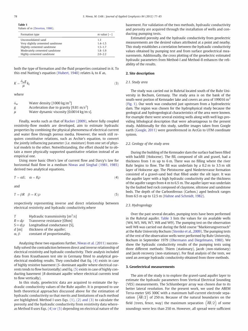
Table 1Values of m (Doveton, 1986).

Formation type m value [−]

Unconsolidated sand 1.3Very slightly cemented sandstone 1.4–1.5Slightly cemented sandstone 1.5–1.7Moderately cemented sandstone 1.8–1.9Highly cemented sandstone 2.0–2.2

78 S. Niwas, M. Celik / Journal of Applied Geophysics 84 (2012) 77–85

both the type of formation and the fluid properties contained in it. Tothis end Nutting's equation (Hubert, 1940) relates kf to K as,

K ¼ δwgμ

kf ð3Þ

where

δw Water density [1000 kg/m3]g Acceleration due to gravity [9.81 m/s2]μ Water dynamic viscosity [0.0014 kg/m s].

Finally, works such as that of Rucker (2009), where fully coupledresistivity‐flow models are developed, aim to estimate hydraulicproperties by combining the physical phenomena of electrical currentand water flow through porous media. However, the work still re-quires constitutive relations, such as Archie's equation, to convertthe jointly influencing parameter (i.e. moisture) from one set of phys-ical models to the other. Notwithstanding, the effort should be to ob-tain a more physically supported quantitative relation instead of anempirical one.

Using more basic Ohm's law of current flow and Darcy's law forhorizontal fluid flow in a medium Niwas and Singhal (1981, 1985)derived two analytical equations,

T ¼ αS; α ¼ Kρ ð4Þ

and

T ¼ βR β ¼ K=ρ ð5Þ

respectively representing inverse and direct relationship betweenelectrical resistivity and hydraulic conductivity,where

T Hydraulic transmissivity [m2/s]R=dρ Transverse resistance [Ohm]S=d/ρ Longitudinal conductance [S],d [m] thickness of the aquifer;α, β constant of proportionality.

Analyzing these two equations further, Niwas et al. (2011) success-fully solved the contradiction between direct and inverse relationship ofelectrical resistivity and hydraulic conductivity. Their analysis includeddata from Krauthausen test site in Germany fitted to analytical geo-electrical modeling results. They concluded that Eq. (4) exists in caseof highly resistive basement (S- dominant aquifer where electrical cur-rents tends toflowhorizontally) and Eq. (5) exists in case of highly con-ducting basement (R-dominant aquifer where electrical currents tendto flow vertically).

In this study, geoelectric data are acquired to estimate the hy-draulic conductivity values of the Ruhr aquifer. It is proposed to useboth theoretical approaches discussed above for the estimation ofhydraulic conductivity so that merits and limitations of each methodare highlighted. Method I uses Eqs. (1), (2) and (3) to calculate theporosity and the hydraulic conductivity from resistivity data where-as Method II uses Eqs. (4) or (5) depending on electrical nature of the

basement. For validation of the two methods, hydraulic conductivityand porosity are acquired through the installation of wells and con-ducting pumping tests.

Estimated porosity and the hydraulic conductivity from geoelectricmeasurements are the desired values attributed at a point and nearby.This study establishes a correlation between the hydraulic conductivityvalues obtained by pumping test and from surface geoelectrical mea-surements. Additionally, the cross plotting of the geoelectric estimatedhydraulic parameters from Method-I and Method-II enhances the reli-ability of the results.

2. Site description

2.1. Study area

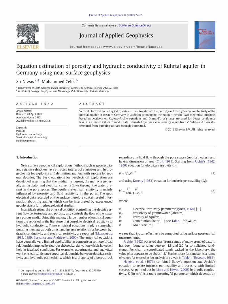
The study was carried out in Ruhrtal located south of the Ruhr Uni-versity in Bochum, Germany. The study area is on the bank of thesouth-west portion of Kemnader lake and covers an area of 199016 m2

(Fig. 1). Our work was conducted just upstream from a hydroelectricdam. The region was chosen for the hydrophysical study because thegeological and hydrogeological characteristics of the area were known.For example there were several existing wells along with well logs pro-viding lithological description that were advantageous to the presentstudy. Additionally for this study, satellite images taken from Googleearth (Google, 2011) were georeferenced in ArcGis to UTM coordinatesystem.

2.2. Geology of the study area

During the building of the Kemnader dam the surface had been filledwith backfill (Holocene). The fill, composed of silt and gravel, had athickness from 1 m up to 6 m. There was no filling where the riverRuhr begins to flow. The fill was underlain by a 0.2 m to 3.5 m siltlayer of Holocene age. The Pleistocene aged Niederterrasse formationconsisted of a gravel-sand bed that filled under the silt layer. It wasthe aquifer layer with a high hydraulic conductivity and the thicknessof the aquifer ranges from4 m to 6.5 m. The aquifer layer was underlainby the faulted bed rock composed of claystone, siltstone and sandstonebeds. The depth of the Carboniferous (Carbon.) aged bedrock rangesfrom 6.5 m up to 12.5 m (Hahne and Schmidt, 1982).

2.3. Hydrogeology

Over the past several decades, pumping tests have been performedin the Ruhrtal aquifer. Table 3 lists the values for six available wells(W4, W5, W6, W7, W8 and W9). The pumping test on the observationwell W8 was carried out during the field course “Markierungsversuch”at the Ruhr University Bochum (Stemke et al., 2009). The pumping testsof the rest of the observation wells were performed by Ruhr University,Bochum in September 1979 (Obermann and Diegelmann, 1980). Weshow the hydraulic conductivity results of the pumping tests usingthree different methods: Thiem (stationary), Jacob (non-stationary)and Jacob recovery (non-stationary). For final analysis of the tests, weused an average hydraulic conductivity obtained from three methods.

3. Geoelectrical measurements

The aim of the study is to explore the gravel-sand aquifer layer toestimate the hydraulic parameters from Vertical Electrical Sounding(VES) measurements. The Schlumberger array was chosen due to itsbetter lateral resolution. For the present work, we used the ABEMTerra-meter SAS 300C with a maximum half-current electrode sepa-ration AB=2

� �of 250 m. Because of the natural boundaries on the

field (trees, fence, way) the maximum separation AB=2� �

of some

soundings were less than 250 m. However, all spread were sufficient

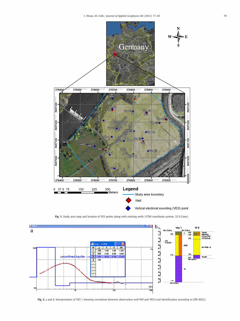
Fig. 1. Study area map and location of VES points along with existing wells (UTM coordinate system, 32 N Zone).

Fig. 2. a and b. Interpretation of VES 1 showing correlation between observation well W9 and VES1(soil identification according to DIN 4022).

79S. Niwas, M. Celik / Journal of Applied Geophysics 84 (2012) 77–85

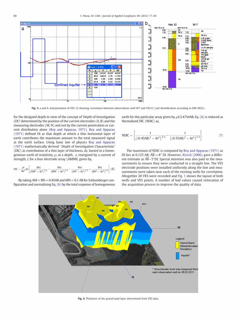
Fig. 3. a and b. Interpretation of VES 12 showing correlation between observations well W7 and VES12 (soil identification according to DIN 4022).

80 S. Niwas, M. Celik / Journal of Applied Geophysics 84 (2012) 77–85

for the designed depth in view of the concept of ‘Depth of Investigation(DI)’ determined by the position of the current electrodes (A, B) and themeasuring electrodes (M, N) and not by the current penetration or cur-rent distribution alone (Roy and Apparao, 1971). Roy and Apparao(1971) defined DI as that depth at which a thin horizontal layer ofearth contributes the maximum amount to the total measured signalat the earth surface. Using basic law of physics Roy and Apparao(1971) mathematically derived ‘ Depth of Investigation Characteristic’(DIC) as contribution of a thin layer of thickness, dz, buried in a homo-geneous earth of resistivity, ρ, at a depth , z, energized by a current ofstrength, I, for a four electrode array (AMNB) given by,

DIC ¼ ρI4π2 dz

8πz

AM2 þ 4z2� �3=2 − 8πz

BM2 þ 4z2� �3=2 − 8πz

AN2 þ 4z2� �3=2 þ 8πz

BN2 þ 4z2� �3=2

" #:ð6Þ

By taking AM=BN=0.45AB andMN=0.1AB for Schlumberger con-figuration and normalizing Eq. (6) by the total response of homogeneous

Fig. 4. Thickness of the gravel/sand l

earth for this particular array given by, ρI/2.475πAB, Eq. (6) is reduced asNormalized DIC (NDIC) as,

NDIC ¼ 1

0:45ABð Þ2 þ 4z2� �3=2 −

1

0:55ABð Þ2 þ 4z2� �3=2

" #: ð7Þ

The maximum of NDIC is computed by Roy and Apparao (1971) asDI lies at 0.125 AB; AB=8* DI. However, Kirsch (2006) gave a differ-ent estimate as AB ~5*DI. Special attention was also paid to the mea-surements to ensure they were conducted in a straight line. The VESelectrode positions were installed uniformly along the line and mea-surements were taken near each of the existing wells for correlation.Altogether 20 VES were recorded and Fig. 1 shows the layout of bothwells and VES points. A number of bad values caused reiteration ofthe acquisition process to improve the quality of data.

ayer determined from VES data.

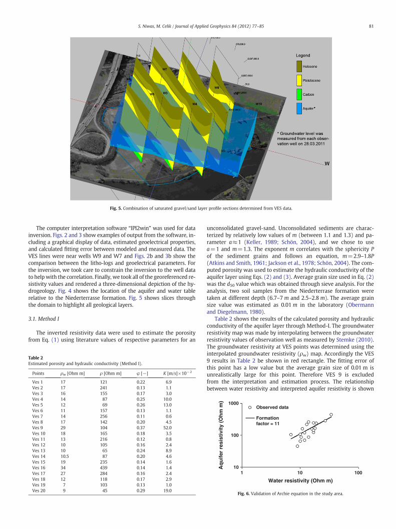
Fig. 5. Combination of saturated gravel/sand layer profile sections determined from VES data.

81S. Niwas, M. Celik / Journal of Applied Geophysics 84 (2012) 77–85

The computer interpretation software “IPI2win” was used for datainversion. Figs. 2 and 3 show examples of output from the software, in-cluding a graphical display of data, estimated geoelectrical properties,and calculated fitting error between modeled and measured data. TheVES lines were near wells W9 and W7 and Figs. 2b and 3b show thecomparison between the litho-logs and geoelectrical parameters. Forthe inversion, we took care to constrain the inversion to the well datato help with the correlation. Finally, we took all of the georeferenced re-sistivity values and rendered a three-dimensional depiction of the hy-drogeology. Fig. 4 shows the location of the aquifer and water tablerelative to the Niederterrasse formation. Fig. 5 shows slices throughthe domain to highlight all geological layers.

3.1. Method I

The inverted resistivity data were used to estimate the porosityfrom Eq. (1) using literature values of respective parameters for an

Table 2Estimated porosity and hydraulic conductivity (Method I).

Points ρw [Ohm m] ρ [Ohm m] φ [−] K [m/s]×10−2

Ves 1 17 121 0.22 6.9Ves 2 17 241 0.13 1.1Ves 3 16 155 0.17 3.0Ves 4 14 87 0.25 10.0Ves 5 12 69 0.26 13.0Ves 6 11 157 0.13 1.1Ves 7 14 256 0.11 0.6Ves 8 17 142 0.20 4.5Ves 9 29 104 0.37 52.0Ves 10 18 165 0.18 3.5Ves 11 13 216 0.12 0.8Ves 12 10 105 0.16 2.4Ves 13 10 65 0.24 8.9Ves 14 10.5 87 0.20 4.6Ves 15 19 235 0.14 1.6Ves 16 34 439 0.14 1.4Ves 17 27 284 0.16 2.4Ves 18 12 118 0.17 2.9Ves 19 7 103 0.13 1.0Ves 20 9 45 0.29 19.0

unconsolidated gravel-sand. Unconsolidated sediments are charac-terized by relatively low values of m (between 1.1 and 1.3) and pa-rameter a≈1 (Keller, 1989; Schön, 2004), and we chose to usea=1 and m=1.3. The exponent m correlates with the sphericity Pof the sediment grains and follows an equation, m=2.9–1.8P(Atkins and Smith, 1961; Jackson et al., 1978; Schön, 2004). The com-puted porosity was used to estimate the hydraulic conductivity of theaquifer layer using Eqs. (2) and (3). Average grain size used in Eq. (2)was the d50 value which was obtained through sieve analysis. For theanalysis, two soil samples from the Niederterrase formation weretaken at different depth (6.7–7 m and 2.5–2.8m). The average grainsize value was estimated as 0.01 m in the laboratory (Obermannand Diegelmann, 1980).

Table 2 shows the results of the calculated porosity and hydraulicconductivity of the aquifer layer through Method-I. The groundwaterresistivity map was made by interpolating between the groundwaterresistivity values of observation well as measured by Stemke (2010).The groundwater resistivity at VES points was determined using theinterpolated groundwater resistivity (ρw) map. Accordingly the VES9 results in Table 2 be shown in red rectangle. The fitting error ofthis point has a low value but the average grain size of 0.01 m isunrealistically large for this point. Therefore VES 9 is excludedfrom the interpretation and estimation process. The relationshipbetween water resistivity and interpreted aquifer resistivity is shown

1000Observed data

Formationfactor = 11

100

101 10

Water resistivity (Ohm m)

Aq

uif

er r

esis

tivi

ty (

Oh

m m

)

100

Fig. 6. Validation of Archie equation in the study area.

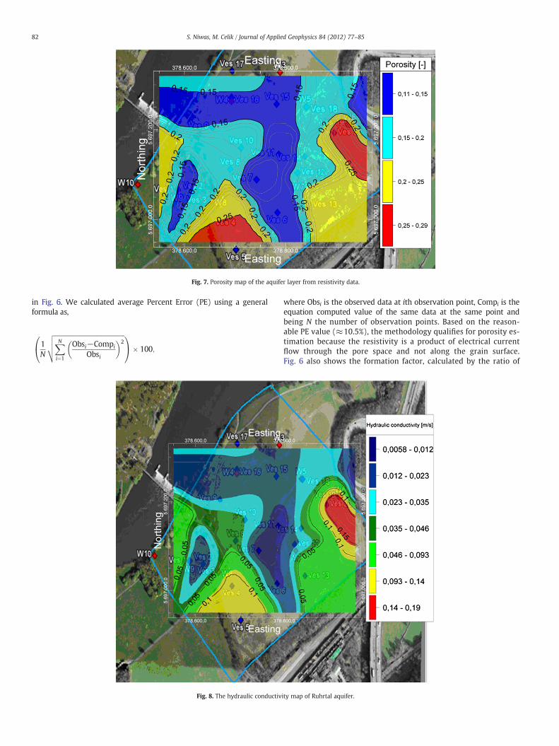
Fig. 7. Porosity map of the aquifer layer from resistivity data.

82 S. Niwas, M. Celik / Journal of Applied Geophysics 84 (2012) 77–85

in Fig. 6. We calculated average Percent Error (PE) using a generalformula as,

1N

ffiffiffiffiffiffiffiffiffiffiffiffiffiffiffiffiffiffiffiffiffiffiffiffiffiffiffiffiffiffiffiffiffiffiffiffiffiffiffiffiffiffiffiffiffiXNi¼1

Obsi−Compi

Obsi

2vuut

0@

1A� 100;

Fig. 8. The hydraulic conductiv

where Obsi is the observed data at ith observation point, Compi is theequation computed value of the same data at the same point andbeing N the number of observation points. Based on the reason-able PE value (≈10.5%), the methodology qualifies for porosity es-timation because the resistivity is a product of electrical currentflow through the pore space and not along the grain surface.Fig. 6 also shows the formation factor, calculated by the ratio of

ity map of Ruhrtal aquifer.

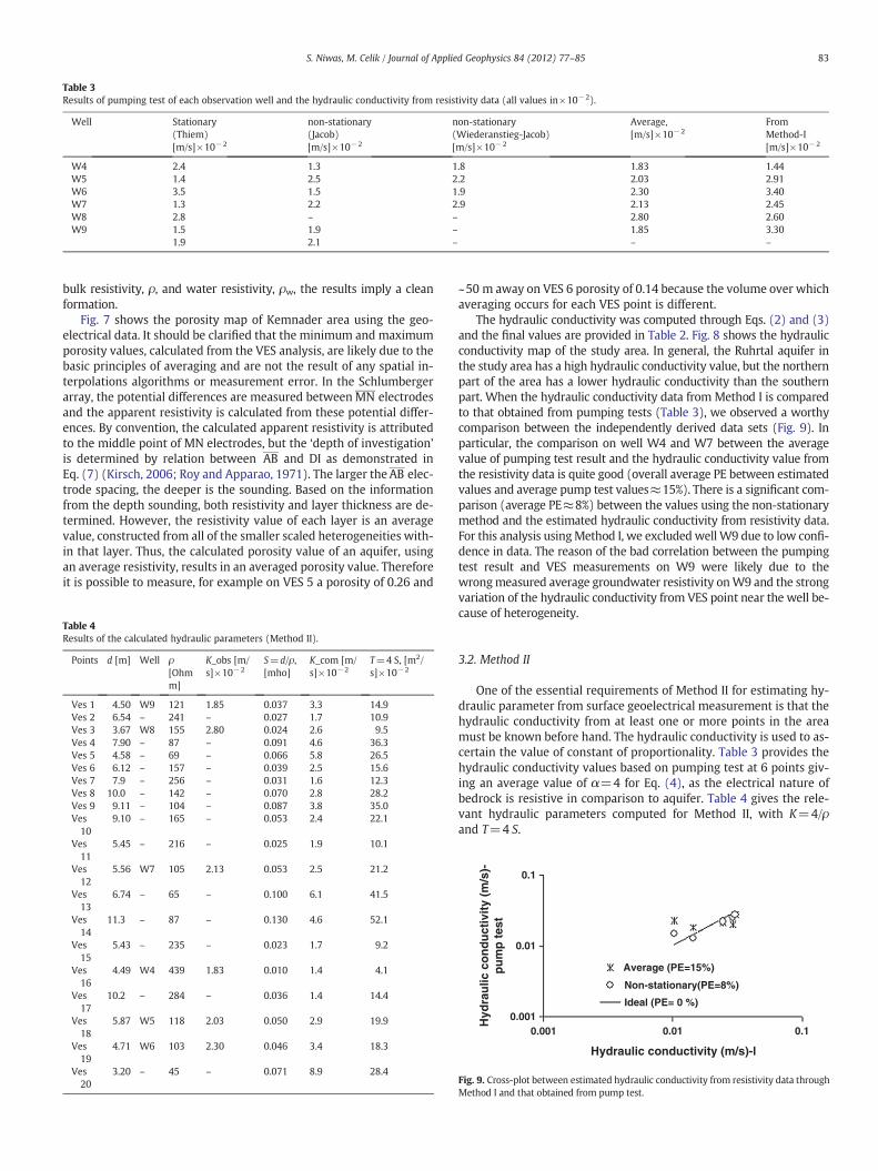
Table 3Results of pumping test of each observation well and the hydraulic conductivity from resistivity data (all values in×10−2).

Well Stationary(Thiem)[m/s]×10−2

non-stationary(Jacob)[m/s]×10−2

non-stationary(Wiederanstieg-Jacob)[m/s]×10−2

Average,[m/s]×10−2

FromMethod-I[m/s]×10−2

W4 2.4 1.3 1.8 1.83 1.44W5 1.4 2.5 2.2 2.03 2.91W6 3.5 1.5 1.9 2.30 3.40W7 1.3 2.2 2.9 2.13 2.45W8 2.8 – – 2.80 2.60W9 1.5 1.9 – 1.85 3.30

1.9 2.1 – – –

83S. Niwas, M. Celik / Journal of Applied Geophysics 84 (2012) 77–85

bulk resistivity, ρ, and water resistivity, ρw, the results imply a cleanformation.

Fig. 7 shows the porosity map of Kemnader area using the geo-electrical data. It should be clarified that the minimum and maximumporosity values, calculated from the VES analysis, are likely due to thebasic principles of averaging and are not the result of any spatial in-terpolations algorithms or measurement error. In the Schlumbergerarray, the potential differences are measured betweenMN electrodesand the apparent resistivity is calculated from these potential differ-ences. By convention, the calculated apparent resistivity is attributedto the middle point of MN electrodes, but the ‘depth of investigation’is determined by relation between AB and DI as demonstrated inEq. (7) (Kirsch, 2006; Roy and Apparao, 1971). The larger theAB elec-trode spacing, the deeper is the sounding. Based on the informationfrom the depth sounding, both resistivity and layer thickness are de-termined. However, the resistivity value of each layer is an averagevalue, constructed from all of the smaller scaled heterogeneities with-in that layer. Thus, the calculated porosity value of an aquifer, usingan average resistivity, results in an averaged porosity value. Thereforeit is possible to measure, for example on VES 5 a porosity of 0.26 and

Table 4Results of the calculated hydraulic parameters (Method II).

Points d [m] Well ρ[Ohmm]

K_obs [m/s]×10−2

S=d/ρ,[mho]

K_com [m/s]×10−2

T=4 S, [m2/s]×10−2

Ves 1 4.50 W9 121 1.85 0.037 3.3 14.9Ves 2 6.54 – 241 – 0.027 1.7 10.9Ves 3 3.67 W8 155 2.80 0.024 2.6 9.5Ves 4 7.90 – 87 – 0.091 4.6 36.3Ves 5 4.58 – 69 – 0.066 5.8 26.5Ves 6 6.12 – 157 – 0.039 2.5 15.6Ves 7 7.9 – 256 – 0.031 1.6 12.3Ves 8 10.0 – 142 – 0.070 2.8 28.2Ves 9 9.11 – 104 – 0.087 3.8 35.0Ves10

9.10 – 165 – 0.053 2.4 22.1

Ves11

5.45 – 216 – 0.025 1.9 10.1

Ves12

5.56 W7 105 2.13 0.053 2.5 21.2

Ves13

6.74 – 65 – 0.100 6.1 41.5

Ves14

11.3 – 87 – 0.130 4.6 52.1

Ves15

5.43 – 235 – 0.023 1.7 9.2

Ves16

4.49 W4 439 1.83 0.010 1.4 4.1

Ves17

10.2 – 284 – 0.036 1.4 14.4

Ves18

5.87 W5 118 2.03 0.050 2.9 19.9

Ves19

4.71 W6 103 2.30 0.046 3.4 18.3

Ves20

3.20 – 45 – 0.071 8.9 28.4

~50 m away on VES 6 porosity of 0.14 because the volume over whichaveraging occurs for each VES point is different.

The hydraulic conductivity was computed through Eqs. (2) and (3)and the final values are provided in Table 2. Fig. 8 shows the hydraulicconductivity map of the study area. In general, the Ruhrtal aquifer inthe study area has a high hydraulic conductivity value, but the northernpart of the area has a lower hydraulic conductivity than the southernpart. When the hydraulic conductivity data from Method I is comparedto that obtained from pumping tests (Table 3), we observed a worthycomparison between the independently derived data sets (Fig. 9). Inparticular, the comparison on well W4 and W7 between the averagevalue of pumping test result and the hydraulic conductivity value fromthe resistivity data is quite good (overall average PE between estimatedvalues and average pump test values≈15%). There is a significant com-parison (average PE≈8%) between the values using the non-stationarymethod and the estimated hydraulic conductivity from resistivity data.For this analysis usingMethod I, we excludedwell W9 due to low confi-dence in data. The reason of the bad correlation between the pumpingtest result and VES measurements on W9 were likely due to thewrongmeasured average groundwater resistivity onW9 and the strongvariation of the hydraulic conductivity from VES point near the well be-cause of heterogeneity.

3.2. Method II

One of the essential requirements of Method II for estimating hy-draulic parameter from surface geoelectrical measurement is that thehydraulic conductivity from at least one or more points in the areamust be known before hand. The hydraulic conductivity is used to as-certain the value of constant of proportionality. Table 3 provides thehydraulic conductivity values based on pumping test at 6 points giv-ing an average value of α=4 for Eq. (4), as the electrical nature ofbedrock is resistive in comparison to aquifer. Table 4 gives the rele-vant hydraulic parameters computed for Method II, with K=4/ρand T=4 S.

0.1

0.1

0.01

0.010.001

0.001

Average (PE=15%)

Non-stationary(PE=8%)

Ideal (PE= 0 %)

Hydraulic conductivity (m/s)-l

Hyd

rau

lic c

on

du

ctiv

ity

(m/s

)-p

um

p t

est

Fig. 9. Cross-plot between estimated hydraulic conductivity from resistivity data throughMethod I and that obtained from pump test.

1.00E+00K values K = 5/Rho

1.00E-01

1.00E-02

1.00E-03

Aquifer resisitivity (Ohm m)

Hyd

rau

lic c

on

du

ctiv

ity

(m/s

)

10 100 1000

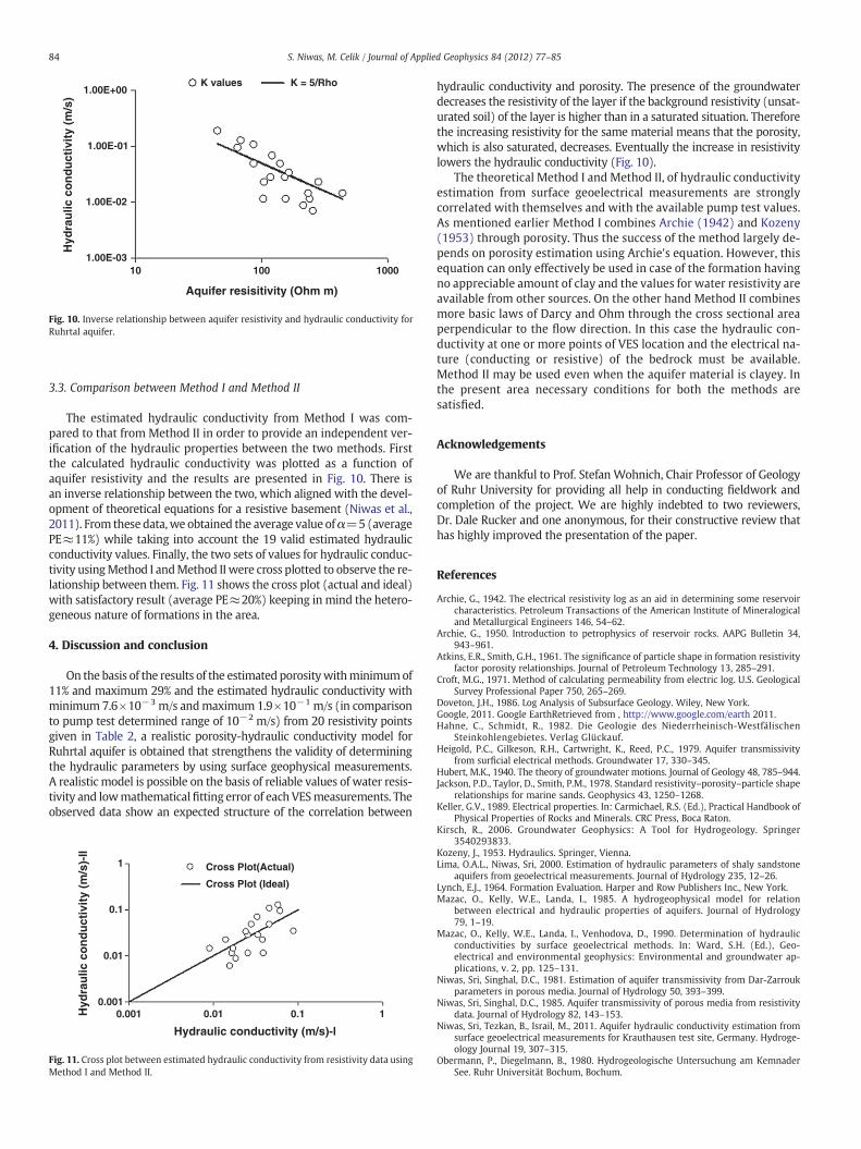
Fig. 10. Inverse relationship between aquifer resistivity and hydraulic conductivity forRuhrtal aquifer.

84 S. Niwas, M. Celik / Journal of Applied Geophysics 84 (2012) 77–85

3.3. Comparison between Method I and Method II

The estimated hydraulic conductivity from Method I was com-pared to that from Method II in order to provide an independent ver-ification of the hydraulic properties between the two methods. Firstthe calculated hydraulic conductivity was plotted as a function ofaquifer resistivity and the results are presented in Fig. 10. There isan inverse relationship between the two, which aligned with the devel-opment of theoretical equations for a resistive basement (Niwas et al.,2011). From these data,we obtained the average value ofα=5(averagePE≈11%) while taking into account the 19 valid estimated hydraulicconductivity values. Finally, the two sets of values for hydraulic conduc-tivity usingMethod I andMethod II were cross plotted to observe the re-lationship between them. Fig. 11 shows the cross plot (actual and ideal)with satisfactory result (average PE≈20%) keeping in mind the hetero-geneous nature of formations in the area.

4. Discussion and conclusion

On the basis of the results of the estimated porositywithminimumof11% and maximum 29% and the estimated hydraulic conductivity withminimum 7.6×10−3 m/s andmaximum 1.9×10−1 m/s (in comparisonto pump test determined range of 10−2 m/s) from 20 resistivity pointsgiven in Table 2, a realistic porosity-hydraulic conductivity model forRuhrtal aquifer is obtained that strengthens the validity of determiningthe hydraulic parameters by using surface geophysical measurements.A realistic model is possible on the basis of reliable values of water resis-tivity and lowmathematicalfitting error of each VESmeasurements. Theobserved data show an expected structure of the correlation between

1

0.1

Cross Plot(Actual)

Cross Plot (Ideal)

0.01

0.0010.001

Hydraulic conductivity (m/s)-l

Hyd

rau

lic c

on

du

ctiv

ity

(m/s

)-ll

0.01 0.1 1

Fig. 11. Cross plot between estimated hydraulic conductivity from resistivity data usingMethod I and Method II.

hydraulic conductivity and porosity. The presence of the groundwaterdecreases the resistivity of the layer if the background resistivity (unsat-urated soil) of the layer is higher than in a saturated situation. Thereforethe increasing resistivity for the same material means that the porosity,which is also saturated, decreases. Eventually the increase in resistivitylowers the hydraulic conductivity (Fig. 10).

The theoretical Method I and Method II, of hydraulic conductivityestimation from surface geoelectrical measurements are stronglycorrelated with themselves and with the available pump test values.As mentioned earlier Method I combines Archie (1942) and Kozeny(1953) through porosity. Thus the success of the method largely de-pends on porosity estimation using Archie's equation. However, thisequation can only effectively be used in case of the formation havingno appreciable amount of clay and the values for water resistivity areavailable from other sources. On the other hand Method II combinesmore basic laws of Darcy and Ohm through the cross sectional areaperpendicular to the flow direction. In this case the hydraulic con-ductivity at one or more points of VES location and the electrical na-ture (conducting or resistive) of the bedrock must be available.Method II may be used even when the aquifer material is clayey. Inthe present area necessary conditions for both the methods aresatisfied.

Acknowledgements

We are thankful to Prof. Stefan Wohnich, Chair Professor of Geologyof Ruhr University for providing all help in conducting fieldwork andcompletion of the project. We are highly indebted to two reviewers,Dr. Dale Rucker and one anonymous, for their constructive review thathas highly improved the presentation of the paper.

References

Archie, G., 1942. The electrical resistivity log as an aid in determining some reservoircharacteristics. Petroleum Transactions of the American Institute of Mineralogicaland Metallurgical Engineers 146, 54–62.

Archie, G., 1950. Introduction to petrophysics of reservoir rocks. AAPG Bulletin 34,943–961.

Atkins, E.R., Smith, G.H., 1961. The significance of particle shape in formation resistivityfactor porosity relationships. Journal of Petroleum Technology 13, 285–291.

Croft, M.G., 1971. Method of calculating permeability from electric log. U.S. GeologicalSurvey Professional Paper 750, 265–269.

Doveton, J.H., 1986. Log Analysis of Subsurface Geology. Wiley, New York.Google, 2011. Google EarthRetrieved from , http://www.google.com/earth 2011.Hahne, C., Schmidt, R., 1982. Die Geologie des Niederrheinisch-Westfälischen

Steinkohlengebietes. Verlag Glückauf.Heigold, P.C., Gilkeson, R.H., Cartwright, K., Reed, P.C., 1979. Aquifer transmissivity

from surficial electrical methods. Groundwater 17, 330–345.Hubert, M.K., 1940. The theory of groundwater motions. Journal of Geology 48, 785–944.Jackson, P.D., Taylor, D., Smith, P.M., 1978. Standard resistivity–porosity–particle shape

relationships for marine sands. Geophysics 43, 1250–1268.Keller, G.V., 1989. Electrical properties. In: Carmichael, R.S. (Ed.), Practical Handbook of

Physical Properties of Rocks and Minerals. CRC Press, Boca Raton.Kirsch, R., 2006. Groundwater Geophysics: A Tool for Hydrogeology. Springer

3540293833.Kozeny, J., 1953. Hydraulics. Springer, Vienna.Lima, O.A.L., Niwas, Sri, 2000. Estimation of hydraulic parameters of shaly sandstone

aquifers from geoelectrical measurements. Journal of Hydrology 235, 12–26.Lynch, E.J., 1964. Formation Evaluation. Harper and Row Publishers Inc., New York.Mazac, O., Kelly, W.E., Landa, I., 1985. A hydrogeophysical model for relation

between electrical and hydraulic properties of aquifers. Journal of Hydrology79, 1–19.

Mazac, O., Kelly, W.E., Landa, I., Venhodova, D., 1990. Determination of hydraulicconductivities by surface geoelectrical methods. In: Ward, S.H. (Ed.), Geo-electrical and environmental geophysics: Environmental and groundwater ap-plications, v. 2, pp. 125–131.

Niwas, Sri, Singhal, D.C., 1981. Estimation of aquifer transmissivity from Dar-Zarroukparameters in porous media. Journal of Hydrology 50, 393–399.

Niwas, Sri, Singhal, D.C., 1985. Aquifer transmissivity of porous media from resistivitydata. Journal of Hydrology 82, 143–153.

Niwas, Sri, Tezkan, B., Israil, M., 2011. Aquifer hydraulic conductivity estimation fromsurface geoelectrical measurements for Krauthausen test site, Germany. Hydroge-ology Journal 19, 307–315.

Obermann, P., Diegelmann, B., 1980. Hydrogeologische Untersuchung am KemnaderSee. Ruhr Universität Bochum, Bochum.

85S. Niwas, M. Celik / Journal of Applied Geophysics 84 (2012) 77–85

Purvance, D.T., Andricevic, R., 2000. On the electric-hydraulic conductivity correlationin aquifers. Water Resources Research 36, 2905–2913.

Roy, A., Apparao, A., 1971. Depth of investigation in direct current methods. Geophysics36, 943–959.

Rucker, D.F., 2009. A coupled electrical resistivity-infiltration model for wetting frontevaluation. Vadose Zone Journal 8, 383–388.

Schön, J.H., 2004. Physical Properties of Rocks. Elsevier, Amsterdam.

Stemke, M., 2010. Labor und Feldversuche zur Desorptionscharakteristik vonFluoreszenzfarbstoffen im Talgrundwasserleiter der Ruhr. Ruhr University, Bochum,Germany.

Stemke, M., Wiesner, B., Celik, M., 2009. Auswertung des Markierungsversuches amKemnader See. Ruhr University, Bochum, Germany.