Journal of Applied Geophysics 126 (2016) 1–12

Contents lists available at ScienceDirect

Journal of Applied Geophysics

j ourna l homepage: www.e lsev ie r .com/ locate / j appgeo

Redatuming controlled-source electromagnetic data using Stratton–Chutype integral transformations

Michael Zhdanov a,b,c, Hongzhu Cai a,⁎a Consortium for Electromagnetic Modeling and Inversion (CEMI), University of Utah, Salt Lake City, UT 84112, USAb TechnoImaging, Salt Lake City, UT 84107, USAc Moscow Institute of Physics and Technology, Moscow 141700, Russia

⁎ Corresponding author.E-mail address: caihongzhu@hotmail.com (H. Cai).

http://dx.doi.org/10.1016/j.jappgeo.2016.01.0030926-9851/© 2016 Elsevier B.V. All rights reserved.

a b s t r a c t

a r t i c l e i n f o

Article history:Received 27 June 2015Received in revised form 2 December 2015Accepted 5 January 2016Available online 9 January 2016

We present a newmethod of analyzing controlled-source electromagnetic (CSEM) data based on redatuming ofthe observed data from the actual receivers into the virtual receivers. We use the Stratton–Chu type integraltransform to calculate the EM field in the virtual receivers. The virtual receivers can be placed at any desirableposition, including close to the target, which increases the sensitivity of the EM data to the target. The developedmethod provides an effective model-based interpolation/extrapolation tool for electromagnetic field data. Thispaper demonstrates that redatuming can be used for designing the optimized CSEM survey configuration. Thenumerical examples, for the Kevin Dome Electromagnetic Project Site, illustrate the practical effectiveness ofthe developed method.

© 2016 Elsevier B.V. All rights reserved.

Keywords:Electromagnetic redatumingAnalytical continuationInterpolationElectromagnetic theory

1. Introduction

The land controlled-source electromagnetic (CSEM) surveys havebeenwidely used inmineral exploration (Zhdanov, 2009, 2010). Duringthe last decade, we have observed also a growing interest in an applica-tion of the marine version of this method to identifying oil- and gas-bearing reservoirs (Constable, 2010). Another emerging technique isbased on using the borehole transmitter and a grid of the surfacereceivers for detailed mapping of the subsurface resistivity of the oil-and gas-producing fields (He et al., 2005, 2010). This method is oftencalled Borehole-to-Surface Electromagnetic (BSEM) surveying. For ex-ample, a successful pilot BSEM field survey was executed recently inSaudi Arabia to identify oil- and water-bearing reservoir layers of a car-bonate oil field water-injection zone (Marsala et al., 2011a, 2011b).

However, the target of the CSEM survey (e.g., BSEM),may be locateddeep underground, which may result in a relatively weak EM responsein the receivers displayed on the surface of the earth. One way to over-come this problem is to move the receivers to the downhole beneaththe overburden and closer to the reservoir target. However, this ap-proach requires using downhole receivers, which is much more techni-cally challenging and expensive than surface observations. In this paperwe propose a numerical approach to estimate the EM field close tothe estimated location of HC reservoir or other potential target. Thisapproach is based on introducing the virtual receivers, located close to

the target, and redatuming the observed data from the actual receiversto the virtual one.

Another possible application of this approach is for solving the datainterpolation and/or extrapolation problem. Themodernmethod for in-terpretation of CSEM survey data is based on a 3D inversion of the ob-served data to estimate the subsurface conductivity distribution. Theresolution of the recovered conductivity is significantly affected by thenumber of available data points on the observation surface, their spatialdensity and the size of the survey area covered by the actual receivers.One method to improve the model resolution of the inversion is to in-crease the number of receivers which requires significantly more effort.This paper develops a numerical method to determine the EM field ina much denser distributed virtual receiver covering the larger area ofobservation, if necessary.

Our developedmethod is based on the ideas of analytical downwardand upward continuation of EM field between the observation surfaceand the surface located closer to a potential target. The principles of an-alytical continuation were originally introduced for the transformationof potential field data, and later on extended for the analytical continu-ation of electromagnetic and seismic field data by Zhdanov (Zhdanov,1988). During the last decades the similar ideas became used in seismicexploration, where they appeared in the form of “redatuming” ofseismic data, or seismic interferometry (Bakulin and Calvert, 2006;Schuster and Zhou, 2006; Schuster, 2009; Wapenaar et al., 2010). Re-cently, the same ideas were re-introduced for EM field continuationunder the name of” electromagnetic interferometry” (Hunziker et al.,2009; Wapenaar et al., 2008). In this paper we demonstrate that thetheory of analytical continuation of the EM field based on classical

2 M. Zhdanov, H. Cai / Journal of Applied Geophysics 126 (2016) 1–12

Stratton–Chu type integrals can be effectively used for solving thisproblem.

The developed EM redatuming theory and method may find a wideapplication in the EM field modeling, interpretation, survey design,interpolation, and extrapolation. In some special case, the method canbe treated as a model-based interpolation.

In this paper, as an example, we consider a typical BSEM survey toillustrate the basic theory of EM redatuming. We also demonstrate theeffectiveness of this method for optimizing the survey configurationfor a geoelectrical model of the Kevin Dome Project Site.

2. Integral representations of the EM field in an inhomogeneousmedium

It was demonstrated by Zhdanov (Zhdanov, 1988), that the Lorentzlemma can be used for deriving the integral representations of the EMfields in inhomogeneous medium similar to the Stratton–Chu formulasfor a homogeneous medium (Berdichevsky and Zhdanov, 1984;Stratton, 1941). We will use here a similar approach to obtain integralrepresentations of the EM field in an inhomogeneous medium.

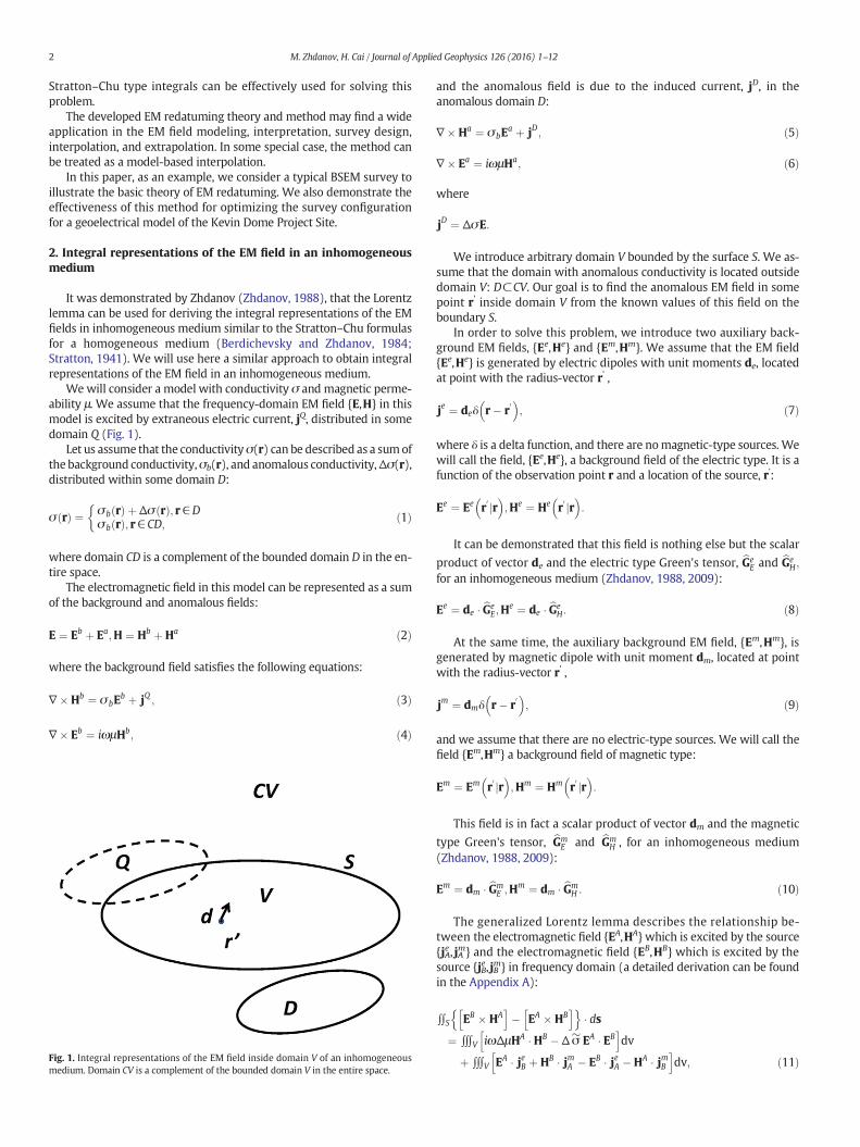
We will consider a model with conductivity σ and magnetic perme-ability μ. We assume that the frequency-domain EM field {E,H} in thismodel is excited by extraneous electric current, jQ, distributed in somedomain Q (Fig. 1).

Let us assume that the conductivityσ(r) can be described as a sumofthe background conductivity,σb(r), and anomalous conductivity,Δσ(r),distributed within some domain D:

σ rð Þ ¼ σb rð Þ þ Δσ rð Þ; r ∈Dσb rð Þ; r ∈ CD;

�ð1Þ

where domain CD is a complement of the bounded domain D in the en-tire space.

The electromagnetic field in this model can be represented as a sumof the background and anomalous fields:

E ¼ Eb þ Ea;H ¼ Hb þ Ha ð2Þ

where the background field satisfies the following equations:

∇�Hb ¼ σbEb þ jQ ; ð3Þ

∇� Eb ¼ iωμHb; ð4Þ

Fig. 1. Integral representations of the EM field inside domain V of an inhomogeneousmedium. Domain CV is a complement of the bounded domain V in the entire space.

and the anomalous field is due to the induced current, jD, in theanomalous domain D:

∇� Ha ¼ σbEa þ jD; ð5Þ

∇� Ea ¼ iωμHa; ð6Þ

where

jD ¼ ΔσE:

We introduce arbitrary domain V bounded by the surface S. We as-sume that the domain with anomalous conductivity is located outsidedomain V: D⊂CV. Our goal is to find the anomalous EM field in somepoint r' inside domain V from the known values of this field on theboundary S.

In order to solve this problem, we introduce two auxiliary back-ground EM fields, {Ee,He} and {Em,Hm}. We assume that the EM field{Ee,He} is generated by electric dipoles with unit moments de, locatedat point with the radius-vector r' ,

je ¼ deδ r� r0

� �; ð7Þ

where δ is a delta function, and there are nomagnetic-type sources. Wewill call the field, {Ee,He}, a background field of the electric type. It is afunction of the observation point r and a location of the source, r':

Ee ¼ Ee r0 jr

� �;He ¼ He r

0 jr� �

:

It can be demonstrated that this field is nothing else but the scalar

product of vector de and the electric type Green's tensor, GbeE and Gbe

H;

for an inhomogeneous medium (Zhdanov, 1988, 2009):

Ee ¼ de � GbeE;H

e ¼ de � GbeH : ð8Þ

At the same time, the auxiliary background EM field, {Em,Hm}, isgenerated by magnetic dipole with unit moment dm, located at pointwith the radius-vector r' ,

jm ¼ dmδ r� r0

� �; ð9Þ

and we assume that there are no electric-type sources. We will call thefield {Em,Hm} a background field of magnetic type:

Em ¼ Em r0 jr

� �;Hm ¼ Hm r

0 jr� �

:

This field is in fact a scalar product of vector dm and the magnetic

type Green's tensor, GbmE and Gbm

H , for an inhomogeneous medium(Zhdanov, 1988, 2009):

Em ¼ dm � GbmE ;H

m ¼ dm � GbmH : ð10Þ

The generalized Lorentz lemma describes the relationship be-tween the electromagnetic field {EA,HA} which is excited by the source{jAe , jAm} and the electromagnetic field {EB,HB} which is excited by thesource {jBe, jBm} in frequency domain (a detailed derivation can be foundin the Appendix A):

∫∫S EB � HAh i

� EA � HBh in o

� ds¼ ∫∫∫V iωΔμHA �HB � Δσ� EA � EB

h idv

þ ∫∫∫V EA � jeB þ HB � jmA � EB � jeA �HA � jmBh i

dv; ð11Þ

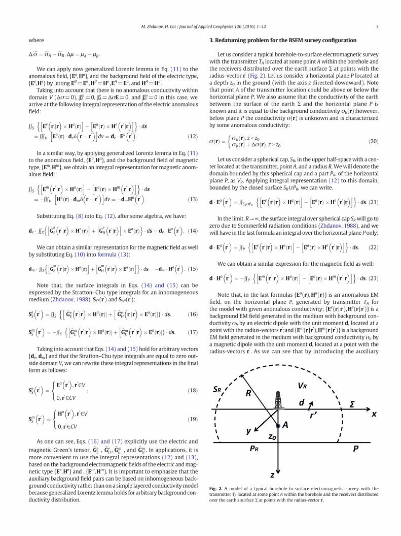
Fig. 2. A model of a typical borehole-to-surface electromagnetic survey with thetransmitter TA located at some point A within the borehole and the receivers distributedover the earth's surface Σ at points with the radius-vector r'.

3M. Zhdanov, H. Cai / Journal of Applied Geophysics 126 (2016) 1–12

where

Δσ� ¼ σ�A � σ�B;Δμ ¼ μA � μB:

We can apply now generalized Lorentz lemma in Eq. (11) to theanomalous field, {Ea,Ha}, and the background field of the electric type,{Ee,He} by letting EB=Ee ,HB=He ,EA=Ea, and HA=Ha.

Taking into account that there is no anomalous conductivity withindomain V (Δσ=0), jAm=0, jAe=ΔσE=0, and jBm=0 in this case, wearrive at the following integral representation of the electric anomalousfield:

∬S Ee r0 jr

� ��Ha rð Þ

h i� Ea rð Þ �He r

0 jr� �h in o

� ds¼ ∭V Ea rð Þ � deδ r� r

0� �h i

dv ¼ de � Ea r0

� �: ð12Þ

In a similar way, by applying generalized Lorentz lemma in Eq. (11)to the anomalous field, {Ea,Ha}, and the background field of magnetictype, {Em,Hm}, we obtain an integral representation formagnetic anom-alous field:

∬S Em r0 jr

� ��Ha rð Þ

h i� Ea rð Þ �Hm r

0 jr� �h in o

� ds¼ �∭V Ha rð Þ � dmδ r� r

0� �h i

dv ¼ �dmHa r0

� �: ð13Þ

Substituting Eq. (8) into Eq. (12), after some algebra, we have:

de � ∫∫S GeE r

0 jr� �

�Ha rð Þh i

þ GeH r

0 jr� �h i

� Ea rð Þn o

� ds ¼ de � Ea r0

� �: ð14Þ

We can obtain a similar representation for themagnetic field aswellby substituting Eq. (10) into formula (13):

dm � ∫∫S GmE r

0 jr� �

�Ha rð Þh i

þ GmH r

0 jr� �

� Ea rð Þh in o

� ds ¼ �dm �Ha r0

� �: ð15Þ

Note that, the surface integrals in Eqs. (14) and (15) can beexpressed by the Stratton–Chu type integrals for an inhomogeneousmedium (Zhdanov, 1988), SEa(r') and SHa(r'):

SeS r0

� �¼ ∬S Gbe

E r0 jr

� ��Ha rð Þ� þ Gbe

H r0 jr

� �� Ea rð Þ�g � ds;

hhnð16Þ

SmS r0

� �¼ �∬S Gbm

E r0 jr

� ��Ha rð Þ� þ Gbm

H r0 jr

� �� Ea rð Þ�g � ds:

hhnð17Þ

Taking into account that Eqs. (14) and (15) hold for arbitrary vectors{de, dm} and that the Stratton–Chu type integrals are equal to zero out-side domain V, we can rewrite these integral representations in the finalform as follows:

SeS r0

� �¼

Ea r0

� �; r

0∈V

0; r0∈CV

8<: ; ð18Þ

SmS r0

� �¼

Ha r0

� �; r

0∈V

0; r0∈CV

8<: ð19Þ

As one can see, Eqs. (16) and (17) explicitly use the electric and

magnetic Green's tensor, GbeE , Gbe

H , GbmE , and Gbm

H . In applications, it ismore convenient to use the integral representations (12) and (13),based on the background electromagnetic fields of the electric andmag-netic type {Ee,He} and , {Em,Hm}. It is important to emphasize that theauxiliary background field pairs can be based on inhomogeneous back-ground conductivity rather than on a simple layered conductivitymodelbecause generalized Lorentz lemmaholds for arbitrary background con-ductivity distribution.

3. Redatuming problem for the BSEM survey configuration

Let us consider a typical borehole-to-surface electromagnetic surveywith the transmitter TA located at some point Awithin the borehole andthe receivers distributed over the earth surface Σ at points with theradius-vector r' (Fig. 2). Let us consider a horizontal plane P located ata depth z0 in the ground (with the axis z directed downward). Notethat point A of the transmitter location could be above or below thehorizontal plane P. We also assume that the conductivity of the earthbetween the surface of the earth Σ and the horizontal plane P isknown and it is equal to the background conductivity σb(r);however,below plane P the conductivity σ(r) is unknown and is characterizedby some anomalous conductivity:

σ rð Þ ¼ σb rð Þ; z b z0σb rð Þ þ Δσ rð Þ; z N z0

�ð20Þ

Let us consider a spherical cap, SR, in the upper half-spacewith a cen-ter located at the transmitter, pointA, and a radius R. Wewill denote thedomain bounded by this spherical cap and a part PR, of the horizontalplane P, as VR. Applying integral representation (12) to this domain,bounded by the closed surface SR∪PR, we can write.

d � Ea r0

� �¼ ∬SR∪PR Ee r

0 jr� �

� Ha rð Þh i

� Ea rð Þ �He r0 jr

� �h in o� ds: ð21Þ

In the limit, R→∞, the surface integral over spherical cap SRwill go tozero due to Sommerfeld radiation conditions (Zhdanov, 1988), and wewill have in the last formula an integral over the horizontal plane P only:

d � Ea r0

� �¼ ∬P Ee r

0 jr� �

� Ha rð Þh i

� Ea rð Þ �He r0 jr

� �h in o� ds: ð22Þ

We can obtain a similar expression for the magnetic field as well:

d �Ha r0

� �¼ �∬P Em r

0 jr� �

� Ha rð Þh i

� Ea rð Þ �Hm r0 jr

� �h in o� ds: ð23Þ

Note that, in the last formulas {Ea(r),Ha(r)} is an anomalous EMfield, on the horizontal plane P, generated by transmitter TA forthe model with given anomalous conductivity; {Ee(r |r'),He(r |r')} is abackground EM field generated in the medium with background con-ductivity σb by an electric dipole with the unit moment d, located at apoint with the radius-vectors r';and {Em(r |r'),Hm(r |r')} is a backgroundEM field generated in the mediumwith background conductivity σb bya magnetic dipole with the unit moment d, located at a point with theradius-vectors r'. As we can see that by introducing the auxiliary

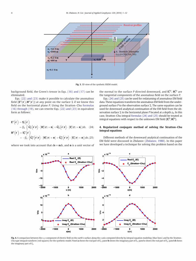
Fig. 3. 3D view of the synthetic BSEM model.

4 M. Zhdanov, H. Cai / Journal of Applied Geophysics 126 (2016) 1–12

background field, the Green's tensor in Eqs. (16) and (17) can beeliminated.

Eqs. (22) and (23) make it possible to calculate the anomalousfield {Ea(r'),Ha(r')} at any point on the surface Σ if we know thisfield on the horizontal plane P. Using the Stratton–Chu formulas(16) through (19), we can rewrite Eqs. (22) and (23) in equivalentform as follows:

Ea r0

� �¼ SeP r

0� �

¼ ∬S GbeE r

0 jr� �

� Haτ rð Þ � n

� �þ GbeH r

0 jr� �

� Eaτ rð Þ � n

� �gds;nð24Þ

Ha r0

� �¼ SmP r

0� �

¼ �∬S GbmE r

0 jr� �

� Haτ rð Þ � n

� �þ GbmH r

0 jr� �

� Eaτ rð Þ � n

� �gds;nð25Þ

where we took into account that ds=nds, and n is a unit vector of

Fig. 4. A comparison between the x, y component of electric field on the earth's surface along thChu type integral transform (red squares) for the syntheticmodel. Panel a shows the real part ofthe imaginary part of Ey.

the normal to the surface P directed downward, and EτPa, Hτ

Pa arethe tangential components of the anomalous field on the surface P.

Eqs. (24) and (25) can be used for redatuming of anomalous EM fielddata. These equations transform the anomalous EMfield from the under-ground surface P to the observation surface Σ. The same equation can beused for downward analytical continuation of the EM field from the ob-servation surface Σ to the horizontal plane P located at a depth z0. In thiscase, Stratton–Chu integral formulas (24) and (25) should be treated asintegral equations with respect to the unknown EM field {EτPa,Hτ

Pa}.

4. Regularized conjugate method of solving the Stratton–Chuintegral equations

Different methods of the downward analytical continuation of theEM field were discussed in Zhdanov (Zhdanov, 1988). In this paperwe have developed a technique for solving this problem based on the

e x axis computed directly by integral equationmodeling (blue lines) and by the Stratton–Ex; panel b shows the imaginary part of Ex; panel c shows the real part of Ey; panel d shows

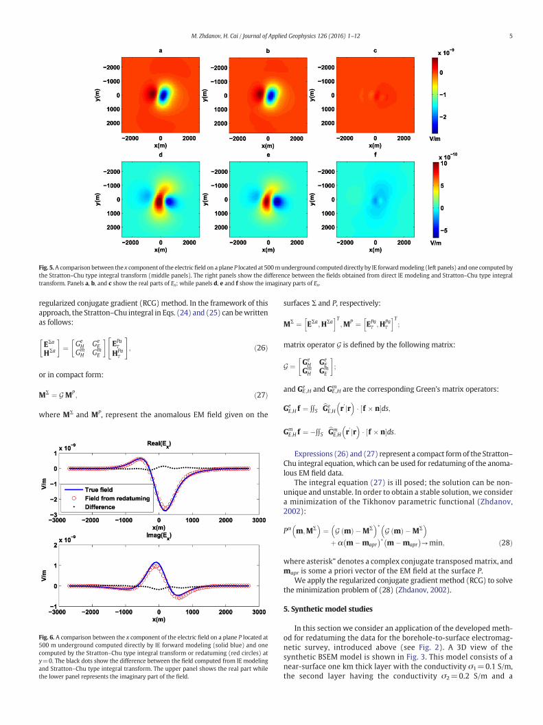
Fig. 5.A comparison between the x component of the electricfield on a plane P located at 500munderground computeddirectly by IE forwardmodeling (left panels) and one computed bythe Stratton–Chu type integral transform (middle panels). The right panels show the difference between the fields obtained from direct IE modeling and Stratton–Chu type integraltransform. Panels a, b, and c show the real parts of Ex; while panels d, e and f show the imaginary parts of Ex.

5M. Zhdanov, H. Cai / Journal of Applied Geophysics 126 (2016) 1–12

regularized conjugate gradient (RCG) method. In the framework of thisapproach, the Stratton–Chu integral in Eqs. (24) and (25) can bewrittenas follows:

EΣa

HΣa

� �¼ Ge

H GeE

GmH Gm

E

� �EPaτ

HPaτ

" #; ð26Þ

or in compact form:

MΣ ¼ G MP ; ð27Þ

where MΣ and MP, represent the anomalous EM field given on the

Fig. 6. A comparison between the x component of the electric field on a plane P located at500 m underground computed directly by IE forward modeling (solid blue) and onecomputed by the Stratton–Chu type integral transform or redatuming (red circles) aty=0. The black dots show the difference between the field computed from IE modelingand Stratton–Chu type integral transform. The upper panel shows the real part whilethe lower panel represents the imaginary part of the field.

surfaces Σ and P, respectively:

MΣ ¼ EΣa;HΣah iT

;MP ¼ EPaτ ;HPa

τ

h iT;

matrix operator G is defined by the following matrix:

G ¼ GeH Ge

EGmH Gm

E

� �;

and GE ,He and GE ,H

m are the corresponding Green's matrix operators:

GeE;H f ¼ ∬S Gbe

E;H r0 jr

� �� f � n½ �ds;

GmE;H f ¼ �∬S Gbm

E;H r0 jr

� �� f � n½ �ds:

Expressions (26) and (27) represent a compact form of the Stratton–Chu integral equation, which can be used for redatuming of the anoma-lous EM field data.

The integral equation (27) is ill posed; the solution can be non-unique and unstable. In order to obtain a stable solution, we considera minimization of the Tikhonov parametric functional (Zhdanov,2002):

Pα m;MΣ� �

¼ G mð Þ �MΣ� ��

G mð Þ �MΣ� �

þ α m�mapr � m�mapr

→min; ð28Þ

where asterisk” denotes a complex conjugate transposedmatrix, andmapr is some a priori vector of the EM field at the surface P.

We apply the regularized conjugate gradient method (RCG) to solvethe minimization problem of (28) (Zhdanov, 2002).

5. Synthetic model studies

In this section we consider an application of the developed meth-od for redatuming the data for the borehole-to-surface electromag-netic survey, introduced above (see Fig. 2). A 3D view of thesynthetic BSEM model is shown in Fig. 3. This model consists of anear-surface one km thick layer with the conductivity σ1=0.1 S/m,the second layer having the conductivity σ2=0.2 S/m and a

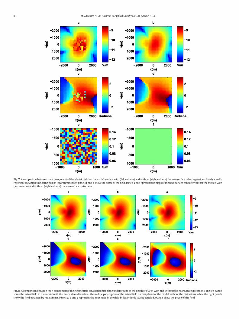
Fig. 7. A comparison between the x component of the electric field on the earth's surface with (left column) and without (right column) the nearsurface inhomogeneities. Panels a and brepresent the amplitude of the field in logarithmic space; panels c and d show the phase of the field. Panels e and f present themaps of the near surface conductivities for themodels with(left column) and without (right column) the nearsurface distortions.

Fig. 8. A comparison between the x component of the electric field on a horizontal plane underground at the depth of 500mwith and without the nearsurface distortions. The left panelsshow the actual field in the model with the nearsurface distortion; the middle panels present the actual field on this plane for the model without the distortions, while the right panelsshow the field obtained by redatuming. Panels a, b and c represent the amplitude of the field in logarithmic space; panels d, e and f show the phase of the field.

6 M. Zhdanov, H. Cai / Journal of Applied Geophysics 126 (2016) 1–12

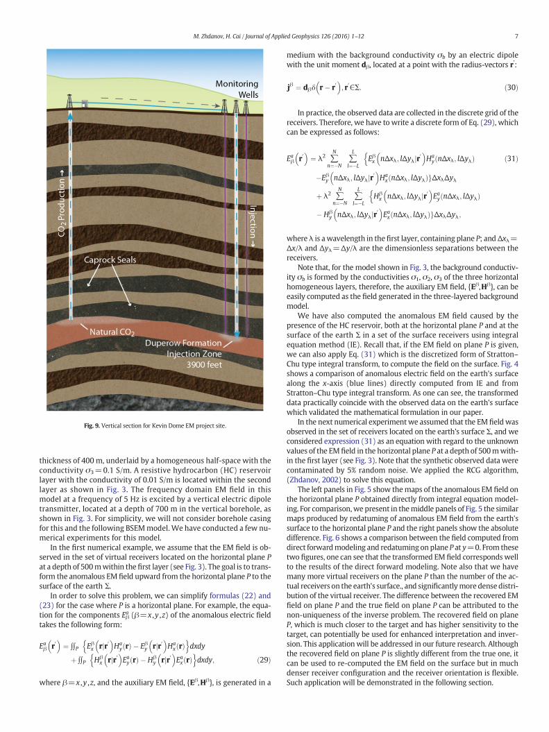
Fig. 9. Vertical section for Kevin Dome EM project site.

7M. Zhdanov, H. Cai / Journal of Applied Geophysics 126 (2016) 1–12

thickness of 400 m, underlaid by a homogeneous half-space with theconductivity σ3=0.1 S/m. A resistive hydrocarbon (HC) reservoirlayer with the conductivity of 0.01 S/m is located within the secondlayer as shown in Fig. 3. The frequency domain EM field in thismodel at a frequency of 5 Hz is excited by a vertical electric dipoletransmitter, located at a depth of 700 m in the vertical borehole, asshown in Fig. 3. For simplicity, we will not consider borehole casingfor this and the following BSEMmodel. We have conducted a few nu-merical experiments for this model.

In the first numerical example, we assume that the EM field is ob-served in the set of virtual receivers located on the horizontal plane Pat a depth of 500mwithin the first layer (see Fig. 3). The goal is to trans-form the anomalous EM field upward from the horizontal plane P to thesurface of the earth Σ.

In order to solve this problem, we can simplify formulas (22) and(23) for the case where P is a horizontal plane. For example, the equa-tion for the components Eβa (β=x ,y ,z) of the anomalous electric fieldtakes the following form:

Eaβ r0

� �¼ ∬P Eβx rjr0

� �Ha

y rð Þ � Eβy rjr0� �

Hax rð Þ

n odxdy

þ ∬P Hβx rjr0� �

Eay rð Þ � Hβy rjr0� �

Eax rð Þn o

dxdy; ð29Þ

where β=x ,y ,z, and the auxiliary EM field, {Eβ,Hβ}, is generated in a

medium with the background conductivity σb by an electric dipolewith the unit moment dβ, located at a point with the radius-vectors r':

jβ ¼ dβδ r� r0

� �; r

0∈Σ: ð30Þ

In practice, the observed data are collected in the discrete grid of thereceivers. Therefore, we have to write a discrete form of Eq. (29), whichcan be expressed as follows:

Eaβ r0

� �¼ λ2 ∑

N

n¼�N∑L

l¼�LEβx nΔxλ; lΔyλjr

0� �

Hay nΔxλ; lΔyλð Þ

n�Eβy nΔxλ; lΔyλjr

0� �

Hax nΔxλ; lΔyλð ÞgΔxλΔyλ

þ λ2 ∑N

n¼�N∑L

l¼�LHβ

x nΔxλ; lΔyλjr0

� �Eay nΔxλ; lΔyλð Þ

n� Hβ

y nΔxλ; lΔyλjr0

� �Eax nΔxλ; lΔyλð ÞgΔxλΔyλ;

ð31Þ

where λ is a wavelength in thefirst layer, containing plane P; andΔxλ=Δx/λ and Δyλ=Δy/λ are the dimensionless separations between thereceivers.

Note that, for the model shown in Fig. 3, the background conductiv-ity σb is formed by the conductivities σ1, σ2, σ3 of the three horizontalhomogeneous layers, therefore, the auxiliary EM field, {Eβ,Hβ}, can beeasily computed as the field generated in the three-layered backgroundmodel.

We have also computed the anomalous EM field caused by thepresence of the HC reservoir, both at the horizontal plane P and at thesurface of the earth Σ in a set of the surface receivers using integralequation method (IE). Recall that, if the EM field on plane P is given,we can also apply Eq. (31) which is the discretized form of Stratton–Chu type integral transform, to compute the field on the surface. Fig. 4shows a comparison of anomalous electric field on the earth's surfacealong the x-axis (blue lines) directly computed from IE and fromStratton–Chu type integral transform. As one can see, the transformeddata practically coincide with the observed data on the earth's surfacewhich validated the mathematical formulation in our paper.

In the next numerical experimentwe assumed that the EM field wasobserved in the set of receivers located on the earth's surface Σ, and weconsidered expression (31) as an equation with regard to the unknownvalues of the EM field in the horizontal plane P at a depth of 500mwith-in the first layer (see Fig. 3). Note that the synthetic observed data werecontaminated by 5% random noise. We applied the RCG algorithm,(Zhdanov, 2002) to solve this equation.

The left panels in Fig. 5 show themaps of the anomalous EM field onthe horizontal plane P obtained directly from integral equation model-ing. For comparison,we present in themiddle panels of Fig. 5 the similarmaps produced by redatuming of anomalous EM field from the earth'ssurface to the horizontal plane P and the right panels show the absolutedifference. Fig. 6 shows a comparison between the field computed fromdirect forwardmodeling and redatumingon plane P at y=0. From thesetwo figures, one can see that the transformed EM field correspondswellto the results of the direct forward modeling. Note also that we havemany more virtual receivers on the plane P than the number of the ac-tual receivers on the earth's surface., and significantlymore dense distri-bution of the virtual receiver. The difference between the recovered EMfield on plane P and the true field on plane P can be attributed to thenon-uniqueness of the inverse problem. The recovered field on planeP, which is much closer to the target and has higher sensitivity to thetarget, can potentially be used for enhanced interpretation and inver-sion. This applicationwill be addressed in our future research. Althoughthe recovered field on plane P is slightly different from the true one, itcan be used to re-computed the EM field on the surface but in muchdenser receiver configuration and the receiver orientation is flexible.Such application will be demonstrated in the following section.

8 M. Zhdanov, H. Cai / Journal of Applied Geophysics 126 (2016) 1–12

Previously, we have assumed that therewere no nearsurface inhomo-geneities in ourmodel and that the EManomalywas caused by the targetonly. In practical application of electromagnetic survey, the measuredfield could be significantly distorted by the nearsurface inhomogeneities,and this effect should be properly treated for the correct interpretation ofthe observed electromagnetic field data (Hördt and Scholl, 2004). Thenearsurface inhomogeneities can be well delineated using conventionalmethods such as DC electric surveys (Zhdanov, 2009) . Our proposedredatuming method provides an approach to reducing the nearsurfacedistortion by downward continuation of the observed field from the sur-face down to a horizontal plane close to the target.

As an example, we have introduced nearsurface inhomogeneitiesrandomly distributed in the 20 m thick nearsurface layer as shown inFig. 7 (panel e). This figure also shows a comparison of the EM fieldson the surfacewith andwithout the effect of the nearsurface inhomoge-neities. For a better comparison, we present the amplitude and phase ofthe fields. One can clearly see the distortions caused by the nearsurfaceinhomogeneities. The left panels of Fig. 8 show the field on the horizon-tal plane at a depth of 500 m for the model with the nearsurface inho-mogeneities, while the middle panels present the field on this planefor the model without the nearsurface distortions. One can clearly seethat the field on the underground plane is less distorted by thenearsurface inhomogeneities comparing to the field observed on theearth's surface. The right panels of this figure show the EM fields onthe underground plane obtained by redatuming for the model withnearsurface distortion. Remarkably, the field produced by redatuming(the right panels) is less distorted by the nearsurface inhomogeneitiesand it is very close to the true field (the left panels). This result

Fig. 10. A 3D resistivity model f

illustrates the robustness of the method for redatuming through theinhomogeneous medium and a possibility of using this technique forreducing the distortion effects of the near surface inhomogeneities.

6. Redatuming for Kevin Dome BSEM project

Kevin Dome is a large underground geological structure in TooleCounty, Montana. The CSEM survey is designed primary to monitor theCO2 sequestration (Zhdanov et al., 2013). In this area, there is an abun-dance of CO2 naturally occurring that has been trapped in places for mil-lions of years indicating strong cap rock formations. Also, CO2 can beextracted from the top portion of the dome and piped a relatively shortdistance down the dome's flank and outside the natural CO2 accumula-tion to the inject site. Fig. 9 is a vertical section for Kevin Dome project.

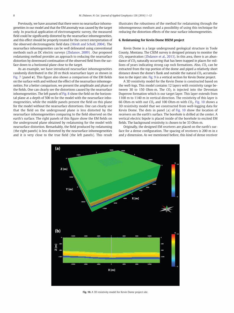
A 3D resistivity model for the Kevin Dome is constructed based onthe well-logs. This model contains 12 layers with resistivity range be-tween 30 to 150 Ohm-m. The CO2 is injected into the DevonianDuperow formation which is our target layer. This layer extends from1100 m to 1140 m in vertical direction. The resistivity of this layer is66 Ohm-m with out CO2 and 100 Ohm-m with CO2. Fig. 10 shows a3D resistivity model that we constructed from well-logging data forKevin Dome. The dots in panel (a) of Fig. 10 show the location ofreceivers on the earth's surface. The borehole is drilled at the center. Avertical electric bipole is placed inside of the borehole to excited EMfields. The background resistivity is chosen to be 33 Ohm-m.

Originally, the designed EM receivers are placed on the earth's sur-face for a dense configuration. The spacing of receivers is 200 m in xand y dimension. As we mentioned before, this kind of dense receiver

or Kevin Dome project site.

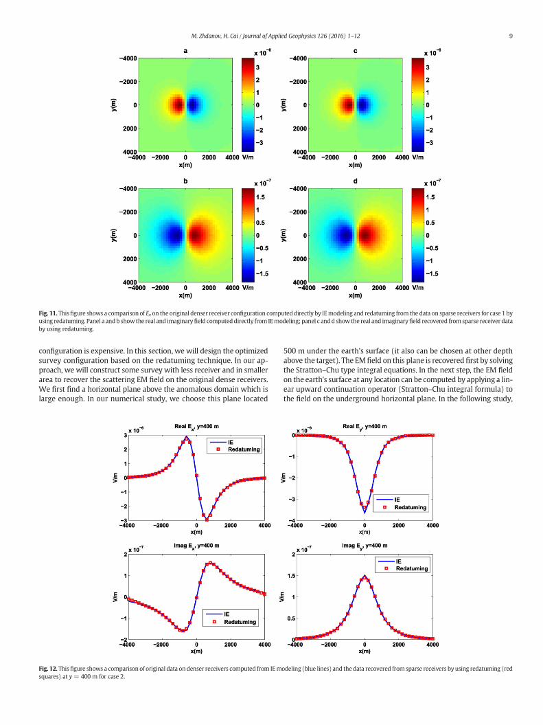
Fig. 11. Thisfigure shows a comparison of Ex on the original denser receiver configuration computed directly by IEmodeling and redatuming from the data on sparse receivers for case 1 byusing redatuming. Panel a andb showthe real and imaginaryfield computed directly from IEmodeling; panel c andd show the real and imaginaryfield recovered from sparse receiver databy using redatuming.

9M. Zhdanov, H. Cai / Journal of Applied Geophysics 126 (2016) 1–12

configuration is expensive. In this section, we will design the optimizedsurvey configuration based on the redatuming technique. In our ap-proach, we will construct some survey with less receiver and in smallerarea to recover the scattering EM field on the original dense receivers.We first find a horizontal plane above the anomalous domain which islarge enough. In our numerical study, we choose this plane located

Fig. 12. Thisfigure shows a comparison of original data on denser receivers computed from IEmsquares) at y = 400 m for case 2.

500 m under the earth's surface (it also can be chosen at other depthabove the target). The EM field on this plane is recovered first by solvingthe Stratton–Chu type integral equations. In the next step, the EM fieldon the earth's surface at any location can be computed by applying a lin-ear upward continuation operator (Stratton–Chu integral formula) tothe field on the underground horizontal plane. In the following study,

odeling (blue lines) and the data recovered from sparse receivers byusing redatuming (red

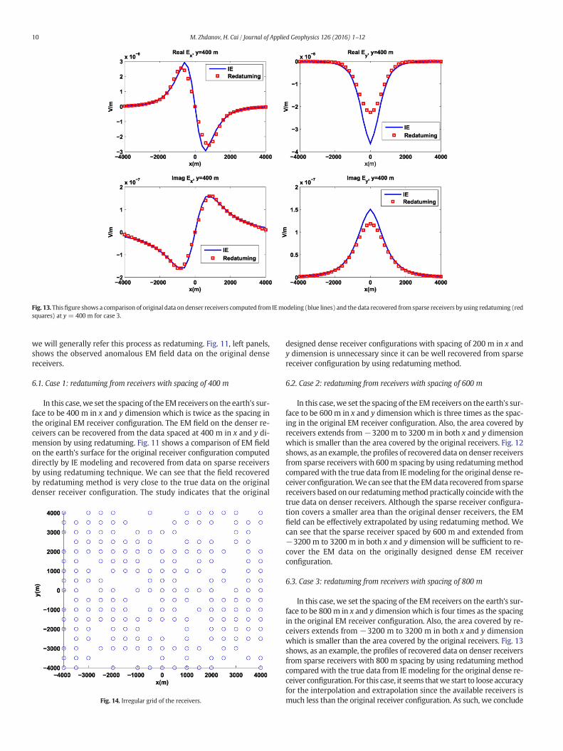
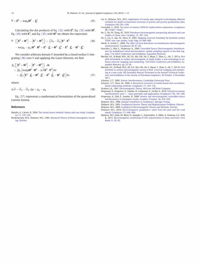
Fig. 13. Thisfigure shows a comparison of original data on denser receivers computed from IEmodeling (blue lines) and the data recovered from sparse receivers byusing redatuming (redsquares) at y = 400 m for case 3.

10 M. Zhdanov, H. Cai / Journal of Applied Geophysics 126 (2016) 1–12

we will generally refer this process as redatuming. Fig. 11, left panels,shows the observed anomalous EM field data on the original densereceivers.

6.1. Case 1: redatuming from receivers with spacing of 400 m

In this case, we set the spacing of the EM receivers on the earth's sur-face to be 400 m in x and y dimension which is twice as the spacing inthe original EM receiver configuration. The EM field on the denser re-ceivers can be recovered from the data spaced at 400 m in x and y di-mension by using redatuming. Fig. 11 shows a comparison of EM fieldon the earth's surface for the original receiver configuration computeddirectly by IE modeling and recovered from data on sparse receiversby using redatuming technique. We can see that the field recoveredby redatuming method is very close to the true data on the originaldenser receiver configuration. The study indicates that the original

Fig. 14. Irregular grid of the receivers.

designed dense receiver configurations with spacing of 200 m in x andy dimension is unnecessary since it can be well recovered from sparsereceiver configuration by using redatuming method.

6.2. Case 2: redatuming from receivers with spacing of 600 m

In this case, we set the spacing of the EM receivers on the earth's sur-face to be 600m in x and y dimension which is three times as the spac-ing in the original EM receiver configuration. Also, the area covered byreceivers extends from−3200 m to 3200 m in both x and y dimensionwhich is smaller than the area covered by the original receivers. Fig. 12shows, as an example, the profiles of recovered data on denser receiversfrom sparse receivers with 600m spacing by using redatumingmethodcomparedwith the true data from IEmodeling for the original dense re-ceiver configuration.We can see that the EMdata recovered fromsparsereceivers based on our redatumingmethod practically coincidewith thetrue data on denser receivers. Although the sparse receiver configura-tion covers a smaller area than the original denser receivers, the EMfield can be effectively extrapolated by using redatuming method. Wecan see that the sparse receiver spaced by 600 m and extended from−3200 m to 3200 m in both x and y dimension will be sufficient to re-cover the EM data on the originally designed dense EM receiverconfiguration.

6.3. Case 3: redatuming from receivers with spacing of 800 m

In this case, we set the spacing of the EM receivers on the earth's sur-face to be 800 m in x and y dimension which is four times as the spacingin the original EM receiver configuration. Also, the area covered by re-ceivers extends from −3200 m to 3200 m in both x and y dimensionwhich is smaller than the area covered by the original receivers. Fig. 13shows, as an example, the profiles of recovered data on denser receiversfrom sparse receivers with 800 m spacing by using redatuming methodcompared with the true data from IE modeling for the original dense re-ceiver configuration. For this case, it seems thatwe start to loose accuracyfor the interpolation and extrapolation since the available receivers ismuch less than the original receiver configuration. As such, we conclude

Fig. 15. This figure shows a comparison of original data on denser receivers computed from IE modeling (blue lines) and the data recovered from sparse and irregular receivers by usingredatuming (red squares) at y = 400 m for case 4.

11M. Zhdanov, H. Cai / Journal of Applied Geophysics 126 (2016) 1–12

that this survey configuration is too sparse and the receiver configurationin case 2 spaced by 600 m is the optimized one for the proposed CSEMsurvey in Kevin Dome EM Project Site.

6.4. Case 4: redatuming from the field observed on irregular distributedreceivers

Previously, we have assumed that the receivers on the earth's sur-face are located on a regular grid. However, in a real case, the receiverscan be deployed on irregular grids only due to various reasons (avail-ability of difficult-to-access areas, costs optimization, etc.). It is wellknown that, using the data observed on a regular grid has a significantadvantage over analyzing the data on an irregular grid in order to pro-duce a robust inversion result (e.g., Cai and Zhdanov, 2015). In this sec-tion, we consider that the data are collected on an irregular grid asshown in Fig. 14 We have applied the redatuming method to recoverthe EM field in the receivers distributed densely on a regular grid.Fig. 15 shows the profiles of recovered data in the densely distributedreceivers in comparison with the true data generated by rigorous IEmodeling on the same regular grid. One can clearly see that the recov-ered EM data on the regular grid are very close to the true data on theregular grid even though the actual receivers were located on a sparseand irregular grid. Thus, we can conclude that redatuming provides amodel based method of interpolation of the EM field data.

7. Conclusions

Wehave developed amethod of redatuming observed EMdata fromactual receivers, located on the earth's surface into virtual receivers lo-cated at depth. Themethod is based on using Stratton–Chu type integraltransforms. The redatuming is achieved by using the regularized conju-gate gradientmethod of solving an ill-posed inverse problem. The appli-cation of the regularization theory makes it possible to apply thismethod to the noisy observed data. We should also emphasize in theconclusion that the developed redatuming method can be used for thecases with the inhomogeneous background conductivity distribution.

We consider an application of thismethod for processing BSEMdata.By placing virtual receivers close to the top of an HC reservoir, we gen-erate the synthetic EM data which can be potentially used for locating

the reservoir. One of the advantages of the redatuming method is thatthe number of virtual receivers can be much bigger than the numberof the actual receivers on the earth's surface. Once the EM field isfound underground by using redatuming, we can use it to re-computethe EM field on the surface but in a much denser receiver configuration.Such approach can be viewed as an model-based interpolation methodfor electromagnetic field. The method can be used to design the opti-mized survey configuration as we demonstrated in the study of KevinDome EM Project Site.

Acknowledgements

The authors acknowledge the University of Utah Consortium forElectromagnetic Modeling and Inversion (CEMI), and TechnoImagingfor the support of this research and permission to publish.

Appendix A. Generalized Lorentz lemma

This appendix reviews the basic theorem characterizing the rela-tionships between the surface and volume distributions of the EM fieldsin arbitrary inhomogeneous media. Let us consider two models of EMparameters distribution, Model A with complex conductivity σ�A andmagnetic permeability μA, and Model B with complex conductivity σ�B

and magnetic permeability μB, respectively. We assume that thefrequency-domain EM field {EA,HA} in Model A is excited by the electricand magnetic sources, {jAe , jAm};while the EM field {EB,HB} in Model B isexcited by the sources, {jBe , jBm}, and that both electromagnetic fieldshave the same frequency ω. These fields satisfy the correspondingMaxwell's equations:

∇� HA ¼ σ�AEA þ jeA; ð32Þ

∇� EA ¼ iωμAHA � jmA ; ð33Þ

∇� HB ¼ σ�BEB þ jeB; ð34Þ

12 M. Zhdanov, H. Cai / Journal of Applied Geophysics 126 (2016) 1–12

∇� EB ¼ iωμBHB � jmB : ð35Þ

Calculating the dot products of Eq. (32) with EB, Eq. (33) with HB,Eq. (34) with EA, and Eq. (35) with HA we obtain the expression

∇ � EB �HAh i

� EA �HBh in o

¼ σ�B � σ�A

� �EA � EB

� iω μB � μAð ÞHA �HB þ EA � jeB þ HB � jmA � EB � jeA �HA � jmB :

ð36Þ

We consider arbitrary domain V, bounded by a closed surface S. Inte-grating (36) over V and applying the Gauss theorem, we find

∫∫S EB �HAh i

� EA �HBh in o

� ds¼ ∫∫∫V iωΔμHA � HB � Δσ�EA � EB

h idv

þ ∫∫∫V EA � jeB þHB � jmA � EB � jeA �HA � jmBh i

dv; ð37Þ

where

Δσ� ¼ σ�A � σ�B;Δμ ¼ μA � μB: ð38Þ

Eq. (37) represents a mathematical formulation of the generalizedLorentz lemma.

References

Bakulin, A., Calvert, R., 2006. The virtual source method: theory and case study. Geophys-ics 71, 139–150.

Berdichevsky, M.N., Zhdanov, M.S., 1984. Advanced Theory of Deep Geomagnetic Sound-ing. Elsevier.

Cai, H., Zhdanov, M.S., 2015. Application of Cauchy-type integrals in developing effectivemethods for depth-to-basement inversion of gravity and gravity gradiometry data.Geophysics 80, G81–G94.

Constable, S., 2010. Ten years of marine CSEM for hydrocarbon exploration. Geophysics75 (75A67–75A81).

He, Z., Hu, W., Dong, W., 2010. Petroleum electromagnetic prospecting advances and casestudies in China. Surv. Geophys. 31, 207–224.

He, Z., Liu, X., Qiu, W., Zhou, H., 2005. Mapping reservoir boundary by borehole surfaceTFEM: two case studies. Lead. Edge 24, 896–900.

Hördt, A., Scholl, C., 2004. The effect of local distortions on timedomain electromagneticmeasurements. Geophysics 69, 87–96.

Hunziker, J., Slob, E., Wapenaar, K., 2009. Controlled Source Electromagnetic Interferom-etry by multidimen-sional deconvolution: spatial sampling aspects in Sea Bed Log-ging. 71st EAGE Conference and Exhibition, Expanded Abstracts.

Marsala, A.F., Al-Buali, M.H., Ali, Z.A., Ma, S.M., He, Z., Biyan, T., Zhao, G.,., He, T., 2011a. Firstpilot of borehole to surface electromagnetic in Saudi Arabia: a new technology to en-hance reservoir mapping and monitoring. 73rd EAGE Conference and Exhibition, Ex-panded Abstracts, pp. 23–26.

Marsala, A.F., Al-Buali, M.H., Ali, Z.A., Ma, S.M., He, Z., Biyan, T., Zhao, G., He, T., 2011b. Firstborehole to surface electromagnetic survey in KSA: reservoir mapping and monitor-ing at a new scale. SPE Extended Abstract Presented at the Annual Technical Confer-ence and Exhibition of the Society of Petroleum Engineers, 30 October–2 November2011.

Schuster, G.T., 2009. Seismic Interferometry. Cambridge University Press.Schuster, G.T., Zhou, M., 2006. A theoretical overview of model-based and correlation-

based redatuming methods. Geophysics 71, 103–110.Stratton, J.A., 1941. Electromagnetic Theory. McGraw-Hill Book Company.Wapenaar, K., Draganov, D., Snieder, R., Campman, X., Verdel, A., 2010. Tutorial on seismic

interferometry: part 1 — basic principles and applications. Geophysics 75A, 195–209.Wapenaar, K., Slob, E., Snieder, R., 2008. Seismic and electromagnetic controlled-source

interferometry in dissipative media. Geophys. Prospect. 56, 419–434.Zhdanov, M.S., 1988. Integral Transforms in Geophysics. Springer-Verlag.Zhdanov, M.S., 2002. Geophysical Inverse Theory and Regularization Problems. Elsevier.Zhdanov, M.S., 2009. Geophysical Electromagnetic Theory and Methods. Elsevier.Zhdanov, M.S., 2010. Electromagnetic geophysics: notes from the past and the road

ahead. Geophysics 75, A49–A66.Zhdanov, M.S., Endo, M., Black, N., Spangler, L., Fairweather, S., Hibbs, A., Eiskamp, G.A., Will,

R., 2013. Electromagnetic monitoring of CO2 sequestration in deep reservoirs. FirstBreak 31, 85–92.