Journal of Applied Geophysics 112 (2015) 175–189

Contents lists available at ScienceDirect

Journal of Applied Geophysics

j ourna l homepage: www.e lsev ie r .com/ locate / j appgeo

Application of EM38 and ERT methods in estimation of saturatedhydraulic conductivity in unsaturated soil

Mohammad Farzamian a,⁎, Fernando A. Monteiro Santos a, Mohamed A. Khalil a,b

a IDL-Universidade de Lisboa, Faculdade de Ciências, Campo Grande, Ed. C8, 1749–016 Lisboa, Portugalb National Research Institute of Astronomy and Geophysics, Helwan, Cairo, Egypt

⁎ Corresponding author. Tel no.: +351217500880.E-mail address: mohammadfarzamian@fc.ul.pt (M. Fa

http://dx.doi.org/10.1016/j.jappgeo.2014.11.0160926-9851/© 2014 Elsevier B.V. All rights reserved.

a b s t r a c t

a r t i c l e i n f o

Article history:Received 27 May 2014Accepted 21 November 2014Available online 29 November 2014

Keywords:ERTEM38Unsaturated flow simulationHydraulic conductivity estimation

Soil apparent electrical conductivity is being considerably used as a surrogatemeasure for soil properties and hy-draulic parameters. In this study, measurements of electrical conductivity were accomplished with electrical re-sistivity tomography (ERT) and EM38 to developmultiple datasets for defining spatiotemporal moisture contentvariations and estimating saturated hydraulic conductivity under natural conditions in an experimental site lo-cated in Lisbon, Portugal. In addition, EM38 capability inmonitoring electrical conductivity variations in compar-ison with ERT method was examined. In order to achieve these objectives, appropriate relationships werederived based on determination of experimental curve resistivity vs. degree of saturation by in-situ investigationto convert electrical resistivity maps inferred from ERT and EM38 data to moisture content distribution maps. Inaddition, the surface temperature variations during the experimentweremeasured and the effects of the temper-ature variations were removed by assuming 2% change in electrical resistivity per °C change in temperature. Theconducted experiment proves that the soil is fairly homogenous and semi-pervious sediment and the spatiotem-poral moisture content variations during the experiment barely exceed 10%. Our calculations constrain the rangeof saturated hydraulic conductivity to be 3–9 (cm/day) range.

© 2014 Elsevier B.V. All rights reserved.

1 . Introduction

The importance of soil characterization in the top 1–2 m is widelyrecognized as a key parameter in agriculture and is critical for optimalcrop management. Development of the means to monitor soil moisturespatiotemporally in agricultural fields is very important for effective soilmoisture management. Moreover, hydraulic conductivity is an impor-tant soil property when determining the potential for water movementin topsoil and in spite of its importance; soil hydraulic conductivity re-mains one of themost difficult of soil properties to assess and laboratorymethods have limitations due to the size of the samples and usually in-situ methods are required to estimate hydraulic conductivity.

Methods of soil moisture determination are often classified into directand indirect methods (Muñoz-Carpena, 2004). Direct methods involvetaking the weight of a soil sample before and after oven drying. Directmethods are based on drilling and causemajor disturbance to the naturalconditions. In addition, direct measurements by sample collection cannotbe repeated over time on the same place, while hydrologic characteriza-tion of topsoil requires a repetition of data collection from a specifiedfield site. Moreover, direct measurements do not usually cover a largearea allowing only localized investigation and cause uncertainty in hydro-logic characterization of unsaturated zone. Due to the destructive nature

rzamian).

of soil sampling, indirect measurements of soil moisture using neutronprobes, capacitance probes and time-domain reflectometry are preferredfor repeated in-situ measurement of soil moisture. These soil moisturesensors have been extensively used in soil water monitoring under awide range of soil types, vegetation and experimental sites (e.g. FaresandAlva, 2000; Fares et al., 2004). Evett et al. (2002) presented a compar-ison of the abovementioned sensors in soil water contentmeasurementsunder a wide range of soil types on four continents to examine the accu-racy and precision of each method and also conditions of successful use.While these in-situ techniques can provide accurate information on soilmoisture, the spatial range of the sensors is limited to tens of centimetersand extension of the information to a large area can be problematic.

Recent research has shown that geophysical methods particularlyground-penetrating radar (GPR), ERT and Electromagnetic inductionmethods (EMI) using non-invasive methods are a viable alternative totraditional techniques for soil characterization. Geophysical methodshave been widely used to investigate unsaturated zone (e.g. Binleyand Kemna, 2005; Binley et al., 2001, 2002a,b; Huisman et al., 2001,2002; Looms et al., 2008a,b; Triantafilis and Monteiro Santos, 2010;Triantafilis et al., 2009). Soil apparent electrical conductivity (ECa) is asurrogate measure for soil properties and can be correlated with soilproperties such as cation exchange capacity (Triantafilis et al., 2009),depth to bedrock and soil texture (Zhu et al., 2010) or clay contentand salinity (Corwin and Lesch, 2005). In addition, time-lapse geophys-ical monitoring is also a powerful tool to estimate those hydrologic

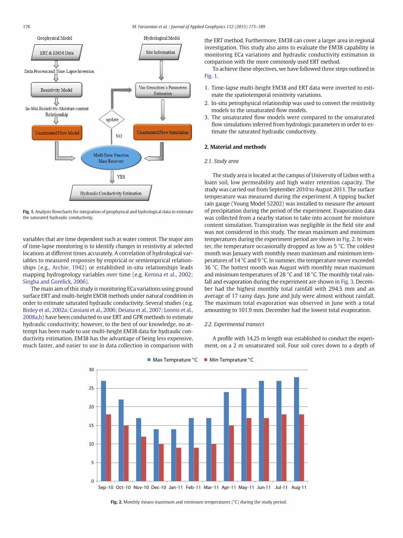
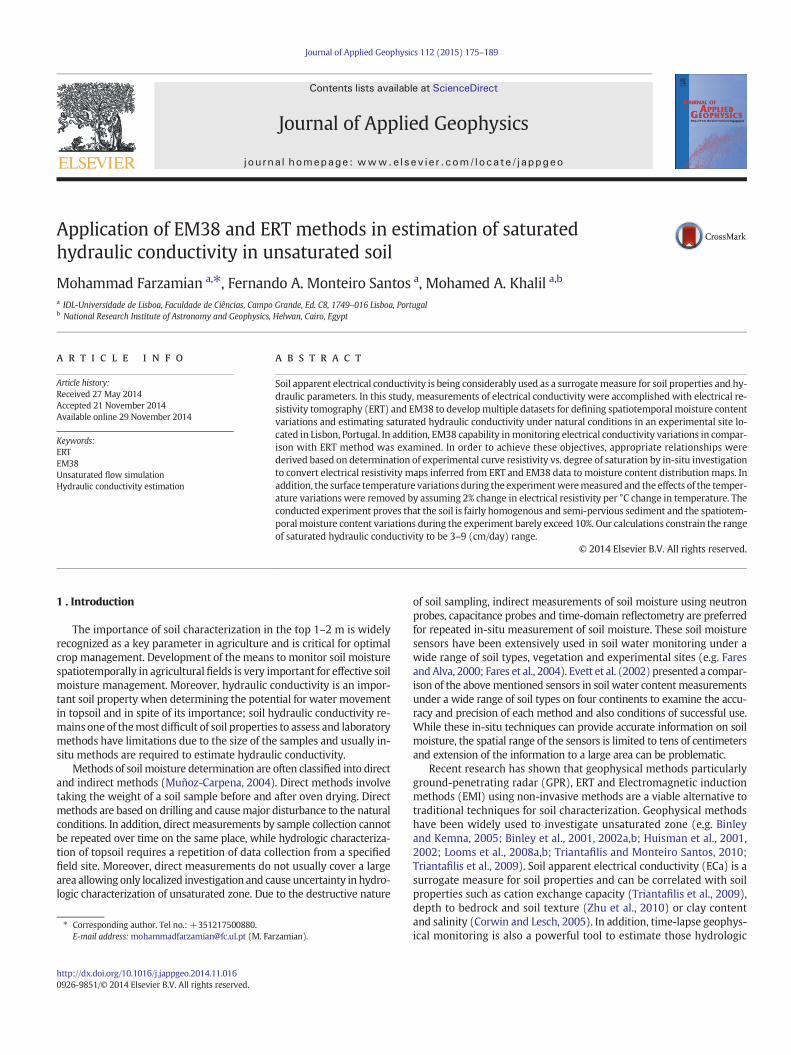
Fig. 1. Analysis flowcharts for integration of geophysical and hydrological data to estimatethe saturated hydraulic conductivity.

176 M. Farzamian et al. / Journal of Applied Geophysics 112 (2015) 175–189

variables that are time dependent such aswater content. Themajor aimof time-lapse monitoring is to identify changes in resistivity at selectedlocations at different times accurately. A correlation of hydrological var-iables to measured responses by empirical or semiempirical relation-ships (e.g., Archie, 1942) or established in-situ relationships leadsmapping hydrogeology variables over time (e.g. Kemna et al., 2002;Singha and Gorelick, 2006).

Themain aimof this study ismonitoring ECa variations using groundsurface ERT andmulti-height EM38methods under natural condition inorder to estimate saturated hydraulic conductivity. Several studies (e.g.Binley et al., 2002a; Cassiani et al., 2006;Deiana et al., 2007; Looms et al.,2008a,b) have been conducted to use ERT and GPRmethods to estimatehydraulic conductivity; however, to the best of our knowledge, no at-tempt has been made to use multi-height EM38 data for hydraulic con-ductivity estimation. EM38 has the advantage of being less expensive,much faster, and easier to use in data collection in comparison with

0

5

10

15

20

25

30

Sep-10 Oct -10 Nov-10 Dec-10 Jan-11 Feb-11

Max Temprature °C

Fig. 2. Monthly means maximum and minimum

the ERT method. Furthermore, EM38 can cover a larger area in regionalinvestigation. This study also aims to evaluate the EM38 capability inmonitoring ECa variations and hydraulic conductivity estimation incomparison with the more commonly used ERT method.

To achieve these objectives,we have followed three steps outlined inFig. 1.

1. Time-lapse multi-height EM38 and ERT data were inverted to esti-mate the spatiotemporal resistivity variations.

2. In-situ petrophysical relationship was used to convert the resistivitymodels to the unsaturated flow models.

3. The unsaturated flow models were compared to the unsaturatedflow simulations inferred from hydrologic parameters in order to es-timate the saturated hydraulic conductivity.

2. Material and methods

2.1. Study area

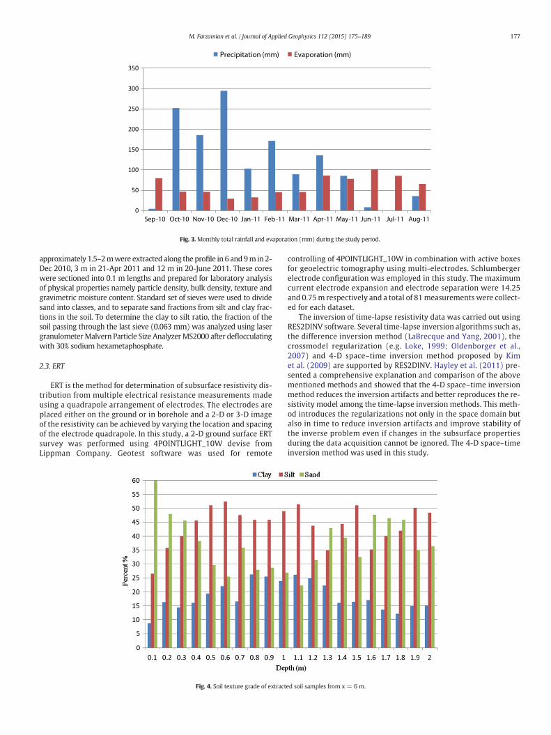
The study area is located at the campus of University of Lisbonwith aloam soil, low permeability and high water retention capacity. Thestudywas carried out from September 2010 to August 2011. The surfacetemperature was measured during the experiment. A tipping bucketrain gauge (Young Model 52202) was installed to measure the amountof precipitation during the period of the experiment. Evaporation datawas collected from a nearby station to take into account for moisturecontent simulation. Transpiration was negligible in the field site andwas not considered in this study. The mean maximum and minimumtemperatures during the experiment period are shown in Fig. 2. In win-ter, the temperature occasionally dropped as low as 5 °C. The coldestmonth was January with monthly meanmaximum and minimum tem-peratures of 14 °C and 9 °C. In summer, the temperature never exceeded36 °C. The hottest month was August with monthly mean maximumandminimum temperatures of 28 °C and 18 °C. The monthly total rain-fall and evaporation during the experiment are shown in Fig. 3. Decem-ber had the highest monthly total rainfall with 294.5 mm and anaverage of 17 rainy days. June and July were almost without rainfall.The maximum total evaporation was observed in June with a totalamounting to 101.9 mm. December had the lowest total evaporation.

2.2. Experimental transect

A profile with 14.25 m length was established to conduct the experi-ment, on a 2 m unsaturated soil. Four soil cores down to a depth of

Mar-11 Apr-11 May-11 Jun-11 Jul-11 Aug-11

Min Temprature °C

temperatures (°C) during the study period.

0

50

100

150

200

250

300

350

Sep-10 Oct-10 Nov-10 Dec-10 Jan-11 Feb-11 Mar-11 Apr-11 May-11 Jun-11 Jul-11 Aug-11

Precipitation (mm) Evaporation (mm)

Fig. 3.Monthly total rainfall and evaporation (mm) during the study period.

177M. Farzamian et al. / Journal of Applied Geophysics 112 (2015) 175–189

approximately 1.5–2mwere extracted along the profile in 6 and9m in 2-Dec 2010, 3 m in 21-Apr 2011 and 12 m in 20-June 2011. These coreswere sectioned into 0.1 m lengths and prepared for laboratory analysisof physical properties namely particle density, bulk density, texture andgravimetric moisture content. Standard set of sieves were used to dividesand into classes, and to separate sand fractions from silt and clay frac-tions in the soil. To determine the clay to silt ratio, the fraction of thesoil passing through the last sieve (0.063 mm) was analyzed using lasergranulometerMalvern Particle Size AnalyzerMS2000 after deflocculatingwith 30% sodium hexametaphosphate.

2.3. ERT

ERT is the method for determination of subsurface resistivity dis-tribution from multiple electrical resistance measurements madeusing a quadrapole arrangement of electrodes. The electrodes areplaced either on the ground or in borehole and a 2-D or 3-D imageof the resistivity can be achieved by varying the location and spacingof the electrode quadrapole. In this study, a 2-D ground surface ERTsurvey was performed using 4POINTLIGHT_10W devise fromLippman Company. Geotest software was used for remote

Fig. 4. Soil texture grade of extract

controlling of 4POINTLIGHT_10W in combination with active boxesfor geoelectric tomography using multi-electrodes. Schlumbergerelectrode configuration was employed in this study. The maximumcurrent electrode expansion and electrode separation were 14.25and 0.75m respectively and a total of 81measurements were collect-ed for each dataset.

The inversion of time-lapse resistivity data was carried out usingRES2DINV software. Several time-lapse inversion algorithms such as,the difference inversion method (LaBrecque and Yang, 2001), thecrossmodel regularization (e.g. Loke, 1999; Oldenborger et al.,2007) and 4-D space–time inversion method proposed by Kimet al. (2009) are supported by RES2DINV. Hayley et al. (2011) pre-sented a comprehensive explanation and comparison of the abovementioned methods and showed that the 4-D space–time inversionmethod reduces the inversion artifacts and better reproduces the re-sistivity model among the time-lapse inversion methods. This meth-od introduces the regularizations not only in the space domain butalso in time to reduce inversion artifacts and improve stability ofthe inverse problem even if changes in the subsurface propertiesduring the data acquisition cannot be ignored. The 4-D space–timeinversion method was used in this study.

ed soil samples from x = 6 m.

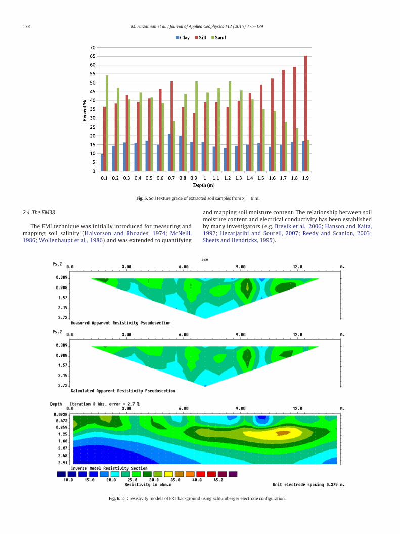
Fig. 5. Soil texture grade of extracted soil samples from x = 9 m.

178 M. Farzamian et al. / Journal of Applied Geophysics 112 (2015) 175–189

2.4. The EM38

The EMI technique was initially introduced for measuring andmapping soil salinity (Halvorson and Rhoades, 1974; McNeill,1986; Wollenhaupt et al., 1986) and was extended to quantifying

Fig. 6. 2-D resistivity models of ERT background

and mapping soil moisture content. The relationship between soilmoisture content and electrical conductivity has been establishedby many investigators (e.g. Brevik et al., 2006; Hanson and Kaita,1997; Hezarjaribi and Sourell, 2007; Reedy and Scanlon, 2003;Sheets and Hendrickx, 1995).

using Schlumberger electrode configuration.

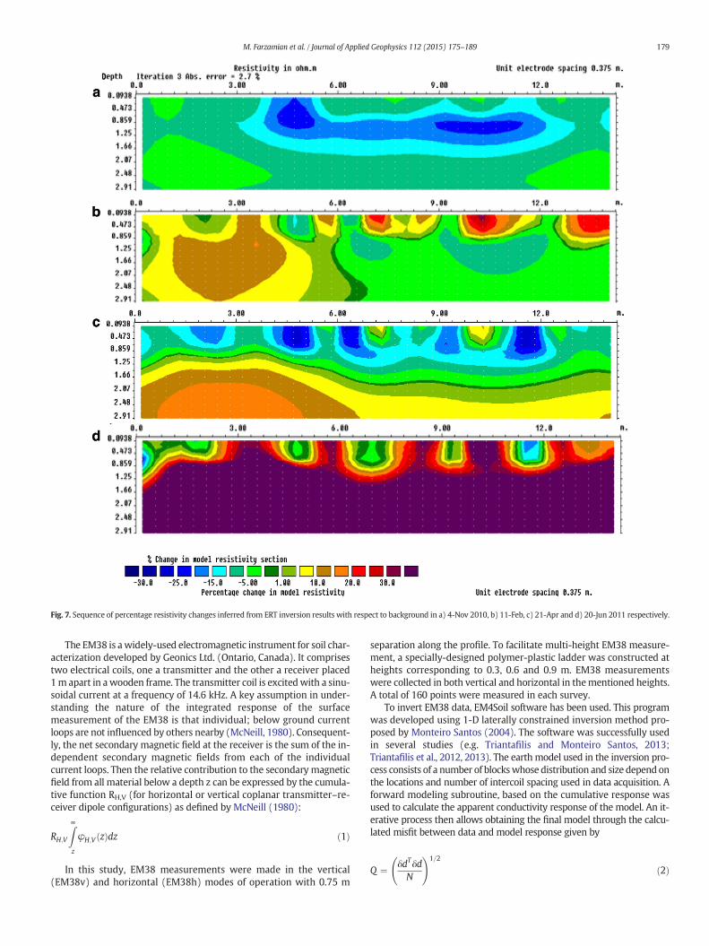
Fig. 7. Sequence of percentage resistivity changes inferred from ERT inversion results with respect to background in a) 4-Nov 2010, b) 11-Feb, c) 21-Apr and d) 20-Jun 2011 respectively.

179M. Farzamian et al. / Journal of Applied Geophysics 112 (2015) 175–189

The EM38 is awidely-used electromagnetic instrument for soil char-acterization developed by Geonics Ltd. (Ontario, Canada). It comprisestwo electrical coils, one a transmitter and the other a receiver placed1m apart in awooden frame. The transmitter coil is excitedwith a sinu-soidal current at a frequency of 14.6 kHz. A key assumption in under-standing the nature of the integrated response of the surfacemeasurement of the EM38 is that individual; below ground currentloops are not influenced by others nearby (McNeill, 1980). Consequent-ly, the net secondary magnetic field at the receiver is the sum of the in-dependent secondary magnetic fields from each of the individualcurrent loops. Then the relative contribution to the secondary magneticfield from all material below a depth z can be expressed by the cumula-tive function RH,V (for horizontal or vertical coplanar transmitter–re-ceiver dipole configurations) as defined by McNeill (1980):

RH;V

Z∞z

φH;V zð Þdz ð1Þ

In this study, EM38 measurements were made in the vertical(EM38v) and horizontal (EM38h) modes of operation with 0.75 m

separation along the profile. To facilitate multi-height EM38 measure-ment, a specially-designed polymer-plastic ladder was constructed atheights corresponding to 0.3, 0.6 and 0.9 m. EM38 measurementswere collected in both vertical and horizontal in thementioned heights.A total of 160 points were measured in each survey.

To invert EM38 data, EM4Soil software has been used. This programwas developed using 1-D laterally constrained inversion method pro-posed by Monteiro Santos (2004). The software was successfully usedin several studies (e.g. Triantafilis and Monteiro Santos, 2013;Triantafilis et al., 2012, 2013). The earth model used in the inversion pro-cess consists of a number of blockswhose distribution and size depend onthe locations and number of intercoil spacing used in data acquisition. Aforward modeling subroutine, based on the cumulative response wasused to calculate the apparent conductivity response of the model. An it-erative process then allows obtaining the final model through the calcu-lated misfit between data and model response given by

Q ¼ δdTδdN

!1=2

ð2Þ

5

10

15

20

25

30

35

40

0 0.75 1.5 2.25 3 3.75 4.5 5.25 6 6.75 7.5 8.25 9 9.75 10.5 11.25 12 12.75 13.5 14.25

ECa

(mS/

m)

X (m)

V₀ H₀ V(0.3m) H(0.3m) V(0.6m) H(0.6m) V(0.9m) H(0.9m)

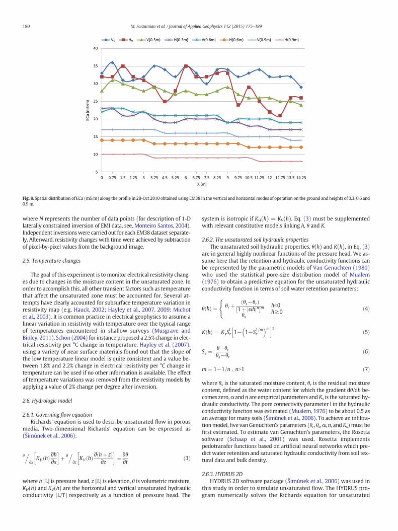
Fig. 8. Spatial distribution of ECa (mS/m) along the profile in 28-Oct 2010 obtained using EM38 in the vertical and horizontalmodes of operation on the ground and heights of 0.3, 0.6 and0.9 m.

180 M. Farzamian et al. / Journal of Applied Geophysics 112 (2015) 175–189

where N represents the number of data points (for description of 1-Dlaterally constrained inversion of EMI data, see, Monteiro Santos, 2004).Independent inversionswere carried out for each EM38 dataset separate-ly. Afterward, resistivity changes with time were achieved by subtractionof pixel-by-pixel values from the background image.

2.5. Temperature changes

The goal of this experiment is to monitor electrical resistivity chang-es due to changes in the moisture content in the unsaturated zone. Inorder to accomplish this, all other transient factors such as temperaturethat affect the unsaturated zone must be accounted for. Several at-tempts have clearly accounted for subsurface temperature variation inresistivity map (e.g. Hauck, 2002; Hayley et al., 2007, 2009; Michotet al., 2003). It is common practice in electrical geophysics to assume alinear variation in resistivity with temperature over the typical rangeof temperatures encountered in shallow surveys (Musgrave andBinley, 2011). Schön (2004) for instance proposed a 2.5% change in elec-trical resistivity per °C change in temperature. Hayley et al. (2007),using a variety of near surface materials found out that the slope ofthe low temperature linear model is quite consistent and a value be-tween 1.8% and 2.2% change in electrical resistivity per °C change intemperature can be used if no other information is available. The effectof temperature variations was removed from the resistivity models byapplying a value of 2% change per degree after inversion.

2.6. Hydrologic model

2.6.1. Governing flow equationRichards' equation is used to describe unsaturated flow in porous

media. Two-dimensional Richards' equation can be expressed as(Šimůnek et al., 2006):

∂.

∂xKH hð Þ ∂h∂x� �

þ ∂.

∂zKV hð Þ ∂ hþ zð Þ

∂z

� �¼ ∂θ

∂t ð3Þ

where h [L] is pressure head, z [L] is elevation, θ is volumetric moisture,KH(h) and KV(h) are the horizontal and vertical unsaturated hydraulicconductivity [L/T] respectively as a function of pressure head. The

system is isotropic if KH(h) = KV(h). Eq. (3) must be supplementedwith relevant constitutive models linking h, θ and K.

2.6.2. The unsaturated soil hydraulic propertiesThe unsaturated soil hydraulic properties, θ(h) and K(h), in Eq. (3)

are in general highly nonlinear functions of the pressure head. We as-sume here that the retention and hydraulic conductivity functions canbe represented by the parametric models of Van Genuchten (1980)who used the statistical pore-size distribution model of Mualem(1976) to obtain a predictive equation for the unsaturated hydraulicconductivity function in terms of soil water retention parameters:

θ hð Þ ¼ θr þθs−θrð Þ

1þ αhj jn½ �mθs

hb0h≥0

8<: ð4Þ

K hð Þ ¼ KsSle 1− 1−S1=me

� �mh i2 ð5Þ

Se ¼θ−θrθs−θr

ð6Þ

m ¼ 1−1=n ; nN1 ð7Þ

where θs is the saturated moisture content, θr is the residual moisturecontent, defined as the water content for which the gradient dθ/dh be-comes zero,α and n are empirical parameters and Ks is the saturated hy-draulic conductivity. The pore connectivity parameter l in the hydraulicconductivity function was estimated (Mualem, 1976) to be about 0.5 asan average for many soils (Šimůnek et al., 2006). To achieve an infiltra-tionmodel, five vanGenuchten's parameters (θr, θs,α, n, and Ks)must befirst estimated. To estimate van Genuchten's parameters, the Rosettasoftware (Schaap et al., 2001) was used. Rosetta implementspedotransfer functions based on artificial neural networks which pre-dict water retention and saturated hydraulic conductivity from soil tex-tural data and bulk density.

2.6.3. HYDRUS 2DHYDRUS 2D software package (Šimůnek et al., 2006) was used in

this study in order to simulate unsaturated flow. The HYDRUS pro-gram numerically solves the Richards equation for unsaturated

Resistivity in ohm.m

a

b

c

d

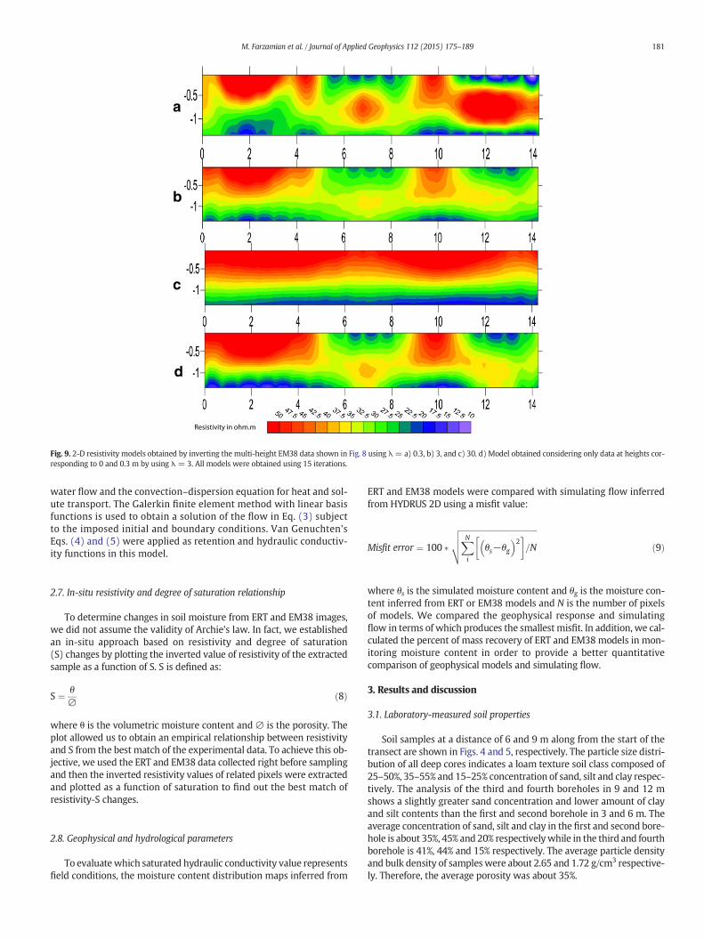
Fig. 9. 2-D resistivity models obtained by inverting the multi-height EM38 data shown in Fig. 8 using λ= a) 0.3, b) 3, and c) 30. d) Model obtained considering only data at heights cor-responding to 0 and 0.3 m by using λ = 3. All models were obtained using 15 iterations.

181M. Farzamian et al. / Journal of Applied Geophysics 112 (2015) 175–189

water flow and the convection–dispersion equation for heat and sol-ute transport. The Galerkin finite element method with linear basisfunctions is used to obtain a solution of the flow in Eq. (3) subjectto the imposed initial and boundary conditions. Van Genuchten'sEqs. (4) and (5) were applied as retention and hydraulic conductiv-ity functions in this model.

2.7. In-situ resistivity and degree of saturation relationship

To determine changes in soil moisture from ERT and EM38 images,we did not assume the validity of Archie's law. In fact, we establishedan in-situ approach based on resistivity and degree of saturation(S) changes by plotting the inverted value of resistivity of the extractedsample as a function of S. S is defined as:

S ¼ θ∅ ð8Þ

where θ is the volumetric moisture content and∅ is the porosity. Theplot allowed us to obtain an empirical relationship between resistivityand S from the best match of the experimental data. To achieve this ob-jective, we used the ERT and EM38 data collected right before samplingand then the inverted resistivity values of related pixels were extractedand plotted as a function of saturation to find out the best match ofresistivity-S changes.

2.8. Geophysical and hydrological parameters

To evaluatewhich saturated hydraulic conductivity value representsfield conditions, the moisture content distribution maps inferred from

ERT and EM38 models were compared with simulating flow inferredfrom HYDRUS 2D using a misfit value:

Misfit error ¼ 100 �ffiffiffiffiffiffiffiffiffiffiffiffiffiffiffiffiffiffiffiffiffiffiffiffiffiffiffiffiffiffiffiffiffiffiffiffiffiffiffiXNi

θs−θg� �2� �

=N

vuut ð9Þ

where θs is the simulated moisture content and θg is the moisture con-tent inferred from ERT or EM38 models and N is the number of pixelsof models. We compared the geophysical response and simulatingflow in terms of which produces the smallest misfit. In addition, we cal-culated the percent of mass recovery of ERT and EM38 models in mon-itoring moisture content in order to provide a better quantitativecomparison of geophysical models and simulating flow.

3. Results and discussion

3.1. Laboratory-measured soil properties

Soil samples at a distance of 6 and 9 m along from the start of thetransect are shown in Figs. 4 and 5, respectively. The particle size distri-bution of all deep cores indicates a loam texture soil class composed of25–50%, 35–55% and 15–25% concentration of sand, silt and clay respec-tively. The analysis of the third and fourth boreholes in 9 and 12 mshows a slightly greater sand concentration and lower amount of clayand silt contents than the first and second borehole in 3 and 6 m. Theaverage concentration of sand, silt and clay in the first and second bore-hole is about 35%, 45% and 20% respectivelywhile in the third and fourthborehole is 41%, 44% and 15% respectively. The average particle densityand bulk density of sampleswere about 2.65 and 1.72 g/cm3 respective-ly. Therefore, the average porosity was about 35%.

Percentage change in model resistivity %

b

a

c

d

e

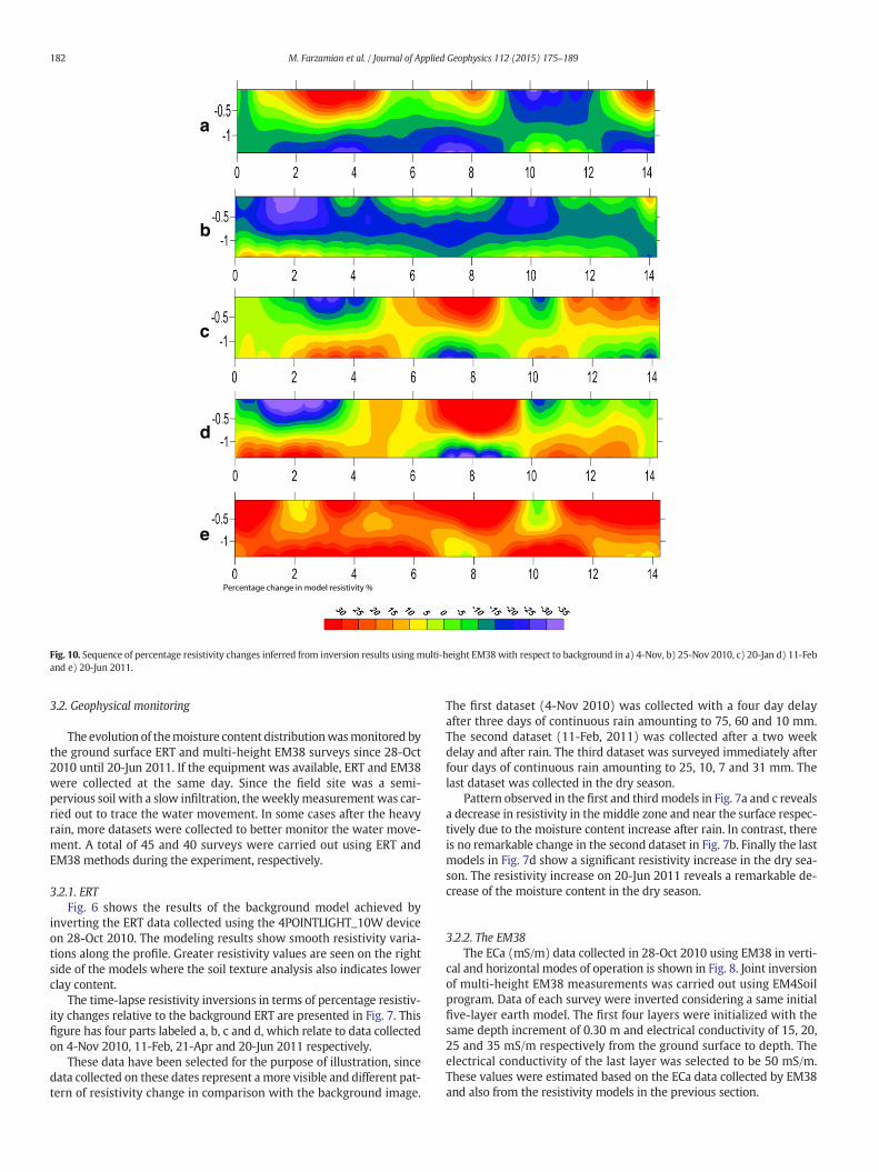
Fig. 10. Sequence of percentage resistivity changes inferred from inversion results using multi-height EM38 with respect to background in a) 4-Nov, b) 25-Nov 2010, c) 20-Jan d) 11-Feband e) 20-Jun 2011.

182 M. Farzamian et al. / Journal of Applied Geophysics 112 (2015) 175–189

3.2. Geophysical monitoring

The evolution of themoisture content distributionwasmonitored bythe ground surface ERT and multi-height EM38 surveys since 28-Oct2010 until 20-Jun 2011. If the equipment was available, ERT and EM38were collected at the same day. Since the field site was a semi-pervious soil with a slow infiltration, the weeklymeasurement was car-ried out to trace the water movement. In some cases after the heavyrain, more datasets were collected to better monitor the water move-ment. A total of 45 and 40 surveys were carried out using ERT andEM38 methods during the experiment, respectively.

3.2.1. ERTFig. 6 shows the results of the background model achieved by

inverting the ERT data collected using the 4POINTLIGHT_10W deviceon 28-Oct 2010. The modeling results show smooth resistivity varia-tions along the profile. Greater resistivity values are seen on the rightside of the models where the soil texture analysis also indicates lowerclay content.

The time-lapse resistivity inversions in terms of percentage resistiv-ity changes relative to the background ERT are presented in Fig. 7. Thisfigure has four parts labeled a, b, c and d, which relate to data collectedon 4-Nov 2010, 11-Feb, 21-Apr and 20-Jun 2011 respectively.

These data have been selected for the purpose of illustration, sincedata collected on these dates represent amore visible and different pat-tern of resistivity change in comparison with the background image.

The first dataset (4-Nov 2010) was collected with a four day delayafter three days of continuous rain amounting to 75, 60 and 10 mm.The second dataset (11-Feb, 2011) was collected after a two weekdelay and after rain. The third dataset was surveyed immediately afterfour days of continuous rain amounting to 25, 10, 7 and 31 mm. Thelast dataset was collected in the dry season.

Pattern observed in the first and thirdmodels in Fig. 7a and c revealsa decrease in resistivity in the middle zone and near the surface respec-tively due to the moisture content increase after rain. In contrast, thereis no remarkable change in the second dataset in Fig. 7b. Finally the lastmodels in Fig. 7d show a significant resistivity increase in the dry sea-son. The resistivity increase on 20-Jun 2011 reveals a remarkable de-crease of the moisture content in the dry season.

3.2.2. The EM38The ECa (mS/m) data collected in 28-Oct 2010 using EM38 in verti-

cal and horizontal modes of operation is shown in Fig. 8. Joint inversionof multi-height EM38 measurements was carried out using EM4Soilprogram. Data of each survey were inverted considering a same initialfive-layer earth model. The first four layers were initialized with thesame depth increment of 0.30 m and electrical conductivity of 15, 20,25 and 35 mS/m respectively from the ground surface to depth. Theelectrical conductivity of the last layer was selected to be 50 mS/m.These values were estimated based on the ECa data collected by EM38and also from the resistivity models in the previous section.

y = 20.243x -1.703

R² = 0.9372

0

50

100

150

200

250

300

350

400

0 0.1 0.2 0.3 0.4 0.5 0.6 0.7 0.8 0.9 1

(ohm

.m)

S

a

y = 24.008x-1.133

R² = 0.8665

0

50

100

150

200

250

0 0.1 0.2 0.3 0.4 0.5 0.6 0.7 0.8 0.9 1

(ohm

.m)

S

b

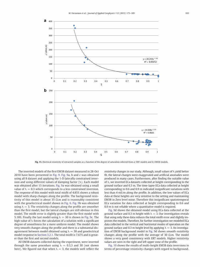
Fig. 11. Electrical resistivity of extracted samples as a function of the degree of saturation inferred from a) ERT models and b) EM38 models.

183M. Farzamian et al. / Journal of Applied Geophysics 112 (2015) 175–189

The invertedmodels of the first EM38 dataset measured in 28-Oct2010 have been presented in Fig. 9. Fig. 9a, b and c was obtainedusing all 8 dataset and applying the 1-D laterally constrained inver-sion and using different values of damping factor (λ). Each modelwas obtained after 15 iterations. Fig. 9a was obtained using a smallvalue of λ = 0.3 which corresponds to a less constrained inversion.The response of this model with total misfit of 4.85% shows a robustmodel with sharp changes along the profile. The background resis-tivity of this model is about 35 Ω.m and is reasonably consistentwith the geoelectrical model shown in Fig. 6. Fig. 9b was obtainedusing λ = 3. The resistivity changes along the profile are smootherthan the first model, but the lateral changes are still obvious in thismodel. The misfit error is slightly greater than the first model with5.18%. Finally the last model using λ = 30 is shown in Fig. 9c. Thehigh value of λ forces the calculation of a solution with a significantdegree of smoothness for a more uniform model. The model showsvery smooth changes along the profile and there is a substantial dis-agreement between model obtained using λ = 30 and geoelectricalmodel response in Section 3.2.1. The total misfit is 7.67% and is great-er than the first and second models.

All EM38 datasets collected during the experiment, were invertedthrough the same procedure using λ = 0.3,3 and 30 (not shownhere). We figured out that when λ = 3, the models well reflect the

resistivity changes in our study. Although, small values of λ yield betterfit, the lateral changes were exaggerated and artificial anomalies wereproduced in many cases. Furthermore, after finding the suitable valueof λ, we inverted ECa datasets collected at height corresponding to theground surface and 0.3 m. The time-lapse ECa data collected at heightcorresponding to 0.6 and 0.9 m indicated insignificant variations withless than 4 mS/m along the profile. In addition, the low values of ECadata at these heights are very sensitive to the setting and maintainingEM38 in Zero level noise. Therefore this insignificant spatiotemporalECa variation for data collected at height corresponding to 0.6 and0.9 m is not reliable where a quantitative model is required.

Fig. 9d shows the obtained model using ECa data collected at theground surface and 0.3 m height with λ = 3. Our investigation revealsthat using only these data reduces the total misfit error and slightly im-proves themodels. Therefore, for further investigation wemodeled ECadata collected in the vertical and horizontal modes of operation on theground surface and 0.3 m height level by applying λ= 3. An investiga-tion of EM38 background model in Fig. 9d shows smooth resistivitychanges along the profile with the average of 30 Ω.m. The modelshows a very good consistency with ERT models. Higher resistivityvalues are seen in the right and left upper zone of the profile.

Fig. 10 shows the results of multi-height EM38 data inversions interms of percentage resistivity changes with regard to background.

a

c

d

e

b

Moisture content %

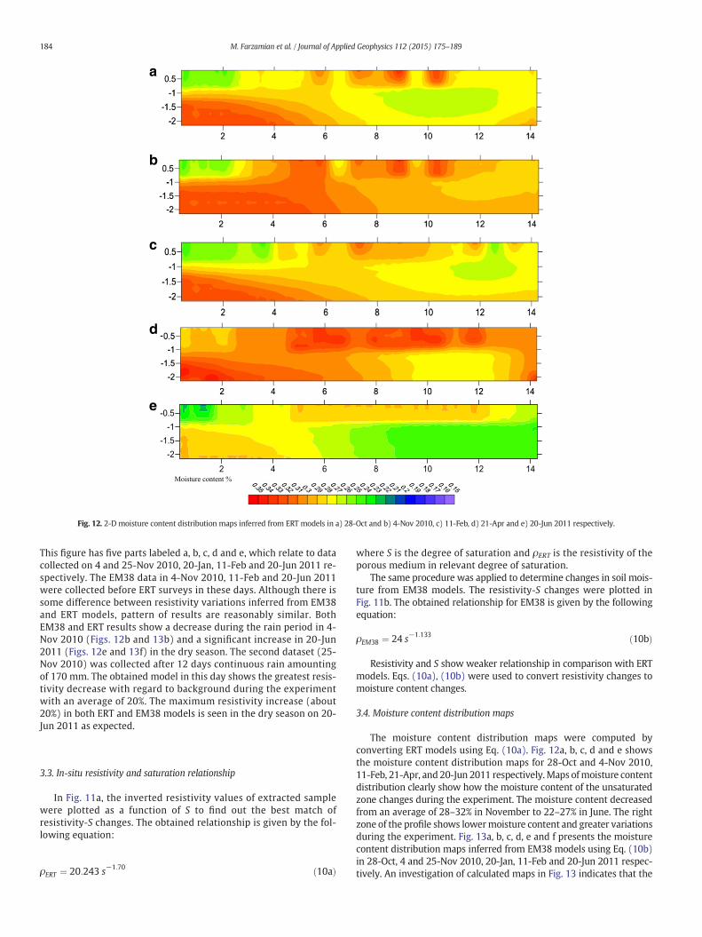
Fig. 12. 2-D moisture content distribution maps inferred from ERT models in a) 28-Oct and b) 4-Nov 2010, c) 11-Feb, d) 21-Apr and e) 20-Jun 2011 respectively.

184 M. Farzamian et al. / Journal of Applied Geophysics 112 (2015) 175–189

This figure has five parts labeled a, b, c, d and e, which relate to datacollected on 4 and 25-Nov 2010, 20-Jan, 11-Feb and 20-Jun 2011 re-spectively. The EM38 data in 4-Nov 2010, 11-Feb and 20-Jun 2011were collected before ERT surveys in these days. Although there issome difference between resistivity variations inferred from EM38and ERT models, pattern of results are reasonably similar. BothEM38 and ERT results show a decrease during the rain period in 4-Nov 2010 (Figs. 12b and 13b) and a significant increase in 20-Jun2011 (Figs. 12e and 13f) in the dry season. The second dataset (25-Nov 2010) was collected after 12 days continuous rain amountingof 170 mm. The obtained model in this day shows the greatest resis-tivity decrease with regard to background during the experimentwith an average of 20%. The maximum resistivity increase (about20%) in both ERT and EM38 models is seen in the dry season on 20-Jun 2011 as expected.

3.3. In-situ resistivity and saturation relationship

In Fig. 11a, the inverted resistivity values of extracted samplewere plotted as a function of S to find out the best match ofresistivity-S changes. The obtained relationship is given by the fol-lowing equation:

ρERT ¼ 20:243 s−1:70 ð10aÞ

where S is the degree of saturation and ρERT is the resistivity of theporous medium in relevant degree of saturation.

The same procedure was applied to determine changes in soil mois-ture from EM38 models. The resistivity-S changes were plotted inFig. 11b. The obtained relationship for EM38 is given by the followingequation:

ρEM38 ¼ 24 s−1:133 ð10bÞ

Resistivity and S show weaker relationship in comparison with ERTmodels. Eqs. (10a), (10b) were used to convert resistivity changes tomoisture content changes.

3.4. Moisture content distribution maps

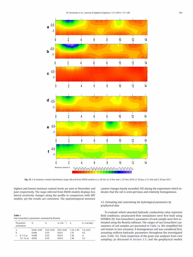
The moisture content distribution maps were computed byconverting ERT models using Eq. (10a). Fig. 12a, b, c, d and e showsthe moisture content distribution maps for 28-Oct and 4-Nov 2010,11-Feb, 21-Apr, and 20-Jun 2011 respectively.Maps ofmoisture contentdistribution clearly show how the moisture content of the unsaturatedzone changes during the experiment. The moisture content decreasedfrom an average of 28–32% in November to 22–27% in June. The rightzone of the profile shows lowermoisture content and greater variationsduring the experiment. Fig. 13a, b, c, d, e and f presents the moisturecontent distribution maps inferred from EM38 models using Eq. (10b)in 28-Oct, 4 and 25-Nov 2010, 20-Jan, 11-Feb and 20-Jun 2011 respec-tively. An investigation of calculated maps in Fig. 13 indicates that the

Moisture content %

a

b

c

d

e

f

Fig. 13. 2-D moisture content distribution maps inferred from EM38 models in a) 28-Oct, b) 4-Nov and c) 25-Nov 2010, d) 20-Jan, e)11-Feb and f) 20-Jun 2011.

185M. Farzamian et al. / Journal of Applied Geophysics 112 (2015) 175–189

highest and lowest moisture content levels are seen in November andJune respectively. The maps inferred from EM38 models displays lesslateral resistivity changes along the profile in comparison with ERTmodels, yet the results are consistent. The spatiotemporal moisture

Table 1Van Genuchten's parameters estimated by Rosetta.

Parameterestimation

θr θs α (cm−1) n ks (cm/day)

a 0.041–0.05 0.33–0.36 0.01–0.02 1.32–1.45 3.5–8.25b 0.046 0.35 0.015 1.35 4.5c 0–7.5 m 0.048 0.35 0.015 1.36 4

7.5–15 m 0.043 0.35 0.014 1.38 5.3

content changes barely exceeded 10% during the experiment which in-dicates that the soil is semi-pervious and relatively homogeneous.

3.5. Estimating and constraining the hydrological parameters bygeophysical data

To evaluate which saturated hydraulic conductivity value representfield conditions, unsaturated flow simulations were first built usingHYDRUS 2D. Van Genuchten's parameters of each sample were first es-timated using the Rosetta software. The ranges of van Genuchten's pa-rameters of soil samples are presented in Table 1a. We simplified thesoil texture to two scenarios. A homogeneous soil was considered first,assuming uniform hydraulic parameters throughout the investigatedarea (Table 1b). Close inspection of the grain size analyses from coresampling (as discussed in Section 3.1) and the geophysical models

0

0.05

0.1

0.15

0.2

0.25

0.3

0 1 2 3 4 5 6 7 8 9 10

Mis

fit e

rror

k=4.5 cm/day K=1 cm/day K=8 cm/day K=16 cm/day

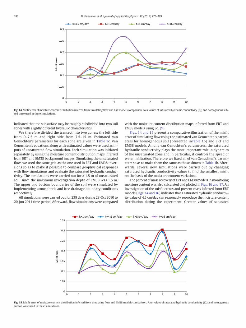
Fig. 14.Misfit error ofmoisture content distribution inferred from simulating flow and ERTmodels comparison. Four values of saturated hydraulic conductivity (Ks) and homogenous sub-soil were used in these simulations.

186 M. Farzamian et al. / Journal of Applied Geophysics 112 (2015) 175–189

indicated that the subsurface may be roughly subdivided into two soilzones with slightly different hydraulic characteristics.

We therefore divided the transect into two zones; the left sidefrom 0–7.5 m and right side from 7.5–15 m. Estimated vanGenuchten's parameters for each zone are given in Table 1c. VanGenuchten's equations along with estimated values were used as in-puts of unsaturated flow simulation. Each simulation was initiatedseparately by using the moisture content distribution maps inferredfrom ERT and EM38 background images. Simulating the unsaturatedflow, we used the same grid as the one used in ERT and EM38 inver-sions so as to make it possible to compare geophysical responseswith flow simulations and evaluate the saturated hydraulic conduc-tivity. The simulations were carried out for a 1.5 m of unsaturatedsoil, since the maximum investigation depth of EM38 was 1.5 m.The upper and bottom boundaries of the soil were simulated byimplementing atmospheric and free drainage boundary conditionsrespectively.

All simulations were carried out for 238 days during 28-Oct 2010 to20-Jun 2011 time period. Afterward, flow simulations were compared

0

0.05

0.1

0.15

0.2

0.25

0.3

0.35

0 1 2 3 4

Mis

fit e

rror

k=1 cm/day k=4.5 cm/day

Fig. 15.Misfit error of moisture content distribution inferred from simulating flow and EM38 msubsoil were used in these simulations.

with the moisture content distribution maps inferred from ERT andEM38 models using Eq. (9).

Figs. 14 and 15 present a comparative illustration of the misfiterror of simulating flow using the estimated van Genuchten's param-eters for homogeneous soil (presented inTable 1b) and ERT andEM38 models. Among van Genuchten's parameters, the saturatedhydraulic conductivity plays the most important role in dynamicsof the unsaturated zone and in particular, it controls the speed ofwater infiltration. Therefore we fixed all of van Genuchten's param-eters so as to make them the same as those shown in Table 1b. After-wards, several new simulations were carried out by changingsaturated hydraulic conductivity values to find the smallest misfiton the basis of the moisture content variations.

The percent ofmass recovery of ERT and EM38models inmonitoringmoisture content was also calculated and plotted in Figs. 16 and 17. Aninvestigation of the misfit errors and present mass inferred from ERTmodels (Figs. 14 and 16) indicates that a saturated hydraulic conductiv-ity value of 4.5 cm/day can reasonably reproduce the moisture contentdistribution during the experiment. Greater values of saturated

5 6 7 8 9 10

k=8 cm/day k=16 cm/day

odels comparison. Four values of saturated hydraulic conductivity (Ks) and homogenous

80

85

90

95

100

105

110

0 1 2 3 4 5 6 7 8 9 10

Perc

ent M

ass

k=4.5 cm/day K=1 cm/day k=8 cm/day k=16 cm/day

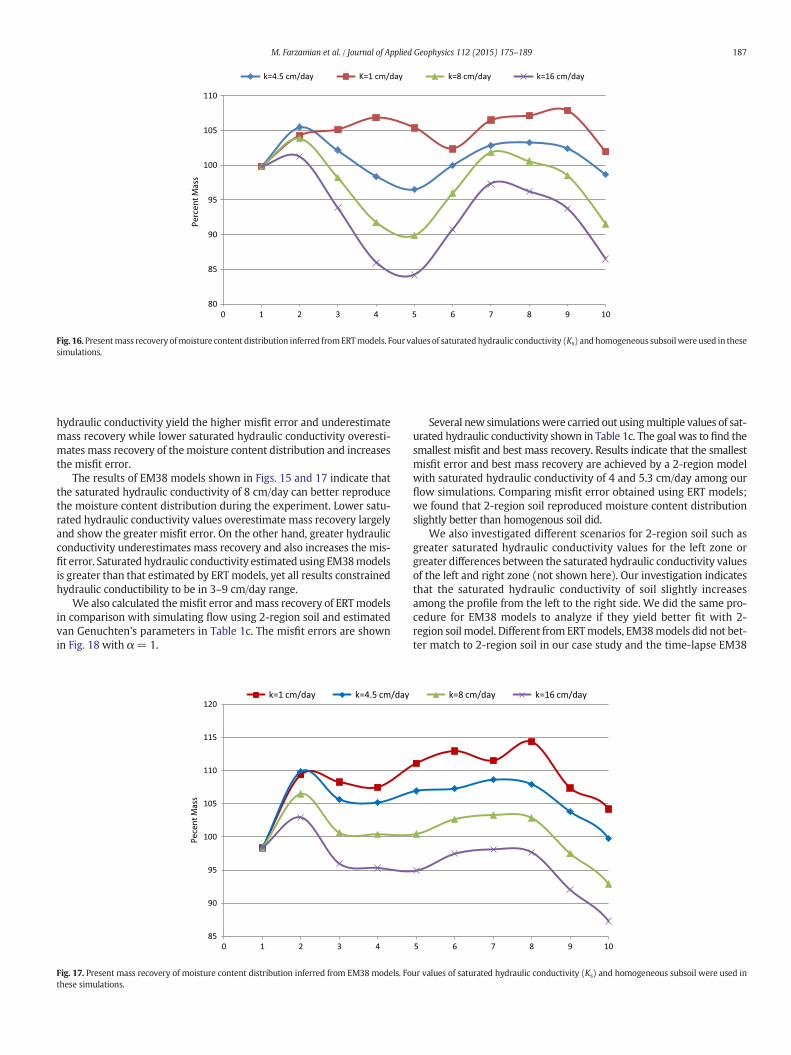
Fig. 16. Presentmass recovery ofmoisture content distribution inferred fromERTmodels. Four values of saturatedhydraulic conductivity (Ks) and homogeneous subsoilwere used in thesesimulations.

187M. Farzamian et al. / Journal of Applied Geophysics 112 (2015) 175–189

hydraulic conductivity yield the higher misfit error and underestimatemass recovery while lower saturated hydraulic conductivity overesti-mates mass recovery of themoisture content distribution and increasesthe misfit error.

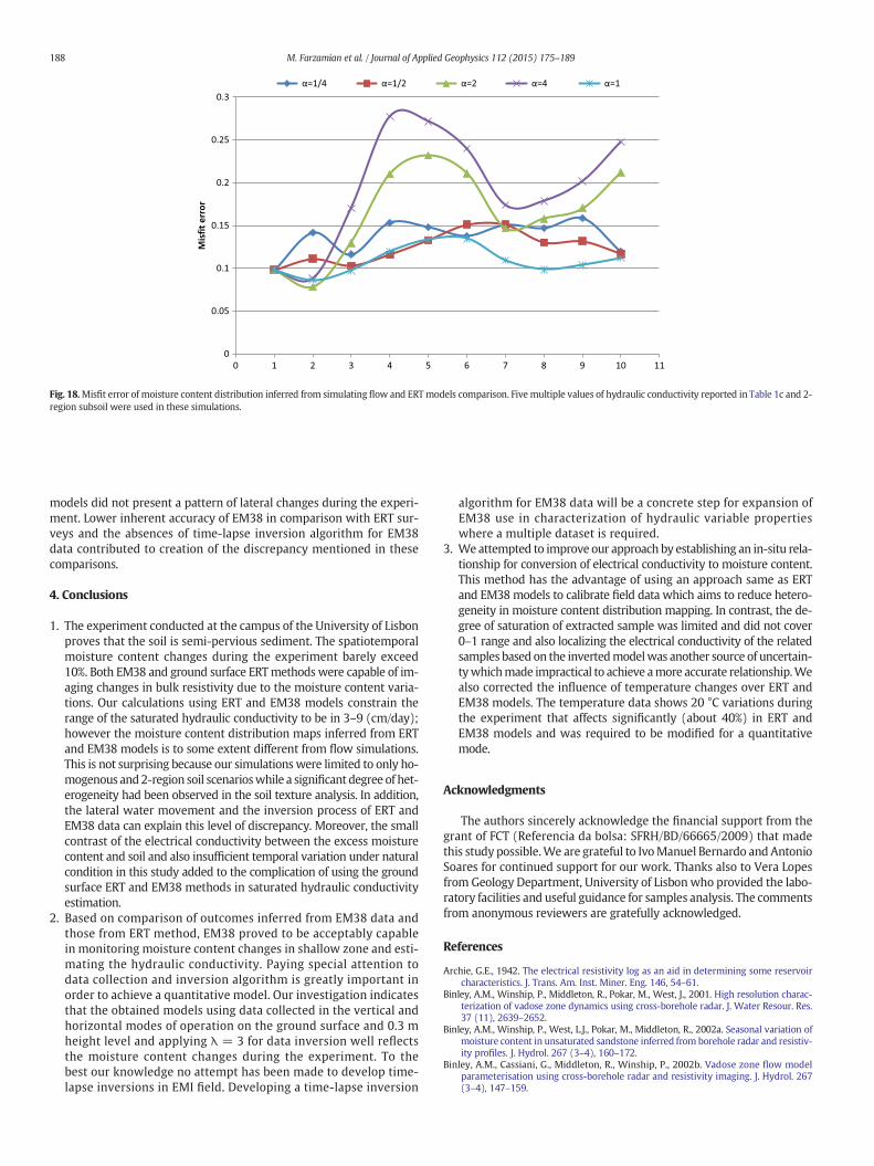
The results of EM38 models shown in Figs. 15 and 17 indicate thatthe saturated hydraulic conductivity of 8 cm/day can better reproducethe moisture content distribution during the experiment. Lower satu-rated hydraulic conductivity values overestimate mass recovery largelyand show the greater misfit error. On the other hand, greater hydraulicconductivity underestimates mass recovery and also increases the mis-fit error. Saturated hydraulic conductivity estimated using EM38modelsis greater than that estimated by ERT models, yet all results constrainedhydraulic conductibility to be in 3–9 cm/day range.

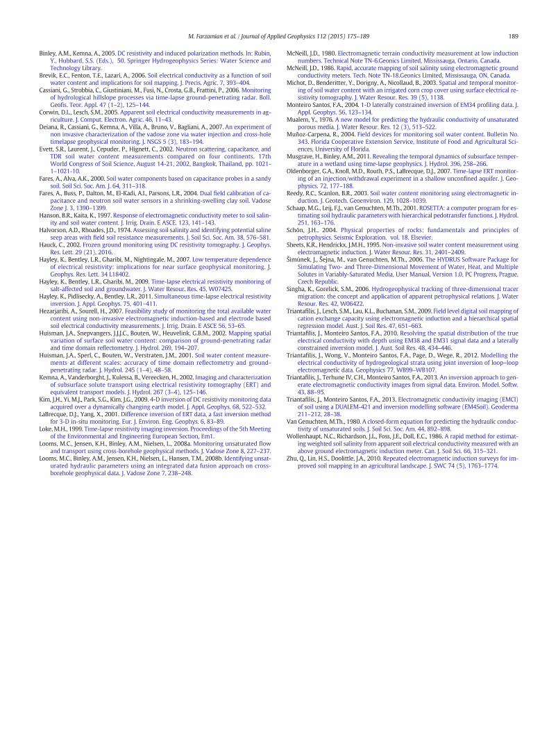
We also calculated themisfit error andmass recovery of ERTmodelsin comparison with simulating flow using 2-region soil and estimatedvan Genuchten's parameters in Table 1c. The misfit errors are shownin Fig. 18 with α = 1.

85

90

95

100

105

110

115

120

0 1 2 3 4

Pece

nt M

ass

k=1 cm/day k=4.5 cm/day

Fig. 17. Present mass recovery of moisture content distribution inferred from EM38 models. Fothese simulations.

Several new simulationswere carried out usingmultiple values of sat-urated hydraulic conductivity shown in Table 1c. The goal was to find thesmallest misfit and best mass recovery. Results indicate that the smallestmisfit error and best mass recovery are achieved by a 2-region modelwith saturated hydraulic conductivity of 4 and 5.3 cm/day among ourflow simulations. Comparing misfit error obtained using ERT models;we found that 2-region soil reproduced moisture content distributionslightly better than homogenous soil did.

We also investigated different scenarios for 2-region soil such asgreater saturated hydraulic conductivity values for the left zone orgreater differences between the saturated hydraulic conductivity valuesof the left and right zone (not shown here). Our investigation indicatesthat the saturated hydraulic conductivity of soil slightly increasesamong the profile from the left to the right side. We did the same pro-cedure for EM38 models to analyze if they yield better fit with 2-region soil model. Different from ERTmodels, EM38models did not bet-ter match to 2-region soil in our case study and the time-lapse EM38

5 6 7 8 9 10

k=8 cm/day k=16 cm/day

ur values of saturated hydraulic conductivity (Ks) and homogeneous subsoil were used in

0

0.05

0.1

0.15

0.2

0.25

0.3

0 1 2 3 4 5 6 7 8 9 10 11

α=1/4 α=1/2 α=2 α=4 α=1

Fig. 18.Misfit error of moisture content distribution inferred from simulating flow and ERTmodels comparison. Five multiple values of hydraulic conductivity reported in Table 1c and 2-region subsoil were used in these simulations.

188 M. Farzamian et al. / Journal of Applied Geophysics 112 (2015) 175–189

models did not present a pattern of lateral changes during the experi-ment. Lower inherent accuracy of EM38 in comparison with ERT sur-veys and the absences of time-lapse inversion algorithm for EM38data contributed to creation of the discrepancy mentioned in thesecomparisons.

4. Conclusions

1. The experiment conducted at the campus of the University of Lisbonproves that the soil is semi-pervious sediment. The spatiotemporalmoisture content changes during the experiment barely exceed10%. Both EM38 and ground surface ERTmethodswere capable of im-aging changes in bulk resistivity due to the moisture content varia-tions. Our calculations using ERT and EM38 models constrain therange of the saturated hydraulic conductivity to be in 3–9 (cm/day);however the moisture content distribution maps inferred from ERTand EM38 models is to some extent different from flow simulations.This is not surprising because our simulations were limited to only ho-mogenous and2-region soil scenarioswhile a significant degree of het-erogeneity had been observed in the soil texture analysis. In addition,the lateral water movement and the inversion process of ERT andEM38 data can explain this level of discrepancy. Moreover, the smallcontrast of the electrical conductivity between the excess moisturecontent and soil and also insufficient temporal variation under naturalcondition in this study added to the complication of using the groundsurface ERT and EM38 methods in saturated hydraulic conductivityestimation.

2. Based on comparison of outcomes inferred from EM38 data andthose from ERT method, EM38 proved to be acceptably capablein monitoring moisture content changes in shallow zone and esti-mating the hydraulic conductivity. Paying special attention todata collection and inversion algorithm is greatly important inorder to achieve a quantitative model. Our investigation indicatesthat the obtained models using data collected in the vertical andhorizontal modes of operation on the ground surface and 0.3 mheight level and applying λ = 3 for data inversion well reflectsthe moisture content changes during the experiment. To thebest our knowledge no attempt has been made to develop time-lapse inversions in EMI field. Developing a time-lapse inversion

algorithm for EM38 data will be a concrete step for expansion ofEM38 use in characterization of hydraulic variable propertieswhere a multiple dataset is required.

3. We attempted to improve our approach by establishing an in-situ rela-tionship for conversion of electrical conductivity to moisture content.This method has the advantage of using an approach same as ERTand EM38models to calibrate field data which aims to reduce hetero-geneity in moisture content distribution mapping. In contrast, the de-gree of saturation of extracted sample was limited and did not cover0–1 range and also localizing the electrical conductivity of the relatedsamples based on the invertedmodelwas another source of uncertain-tywhichmade impractical to achieve amore accurate relationship.Wealso corrected the influence of temperature changes over ERT andEM38 models. The temperature data shows 20 °C variations duringthe experiment that affects significantly (about 40%) in ERT andEM38 models and was required to be modified for a quantitativemode.

Acknowledgments

The authors sincerely acknowledge the financial support from thegrant of FCT (Referencia da bolsa: SFRH/BD/66665/2009) that madethis study possible.We are grateful to IvoManuel Bernardo and AntonioSoares for continued support for our work. Thanks also to Vera Lopesfrom Geology Department, University of Lisbon who provided the labo-ratory facilities and useful guidance for samples analysis. The commentsfrom anonymous reviewers are gratefully acknowledged.

References

Archie, G.E., 1942. The electrical resistivity log as an aid in determining some reservoircharacteristics. J. Trans. Am. Inst. Miner. Eng. 146, 54–61.

Binley, A.M., Winship, P., Middleton, R., Pokar, M., West, J., 2001. High resolution charac-terization of vadose zone dynamics using cross-borehole radar. J. Water Resour. Res.37 (11), 2639–2652.

Binley, A.M., Winship, P., West, L.J., Pokar, M., Middleton, R., 2002a. Seasonal variation ofmoisture content in unsaturated sandstone inferred from borehole radar and resistiv-ity profiles. J. Hydrol. 267 (3–4), 160–172.

Binley, A.M., Cassiani, G., Middleton, R., Winship, P., 2002b. Vadose zone flow modelparameterisation using cross-borehole radar and resistivity imaging. J. Hydrol. 267(3–4), 147–159.

189M. Farzamian et al. / Journal of Applied Geophysics 112 (2015) 175–189

Binley, A.M., Kemna, A., 2005. DC resistivity and induced polarization methods. In: Rubin,Y., Hubbard, S.S. (Eds.), 50. Springer Hydrogeophysics Series: Water Science andTechnology Library.

Brevik, E.C., Fenton, T.E., Lazari, A., 2006. Soil electrical conductivity as a function of soilwater content and implications for soil mapping. J. Precis. Agric. 7, 393–404.

Cassiani, G., Strobbia, C., Giustiniani, M., Fusi, N., Crosta, G.B., Frattini, P., 2006. Monitoringof hydrological hillslope processes via time-lapse ground-penetrating radar. Boll.Geofis. Teor. Appl. 47 (1–2), 125–144.

Corwin, D.L., Lesch, S.M., 2005. Apparent soil electrical conductivity measurements in ag-riculture. J. Comput. Electron. Agric. 46, 11–43.

Deiana, R., Cassiani, G., Kemna, A., Villa, A., Bruno, V., Bagliani, A., 2007. An experiment ofnon invasive characterization of the vadose zone via water injection and cross-holetimelapse geophysical monitoring. J. NSGS 5 (3), 183–194.

Evett, S.R., Laurent, J., Cepuder, P., Hignett, C., 2002. Neutron scattering, capacitance, andTDR soil water content measurements compared on four continents. 17thWorld Congress of Soil Science, August 14-21, 2002, Bangkok, Thailand, pp. 1021-1–1021-10.

Fares, A., Alva, A.K., 2000. Soil water components based on capacitance probes in a sandysoil. Soil Sci. Soc. Am. J. 64, 311–318.

Fares, A., Buss, P., Dalton, M., El-Kadi, A.I., Parsons, L.R., 2004. Dual field calibration of ca-pacitance and neutron soil water sensors in a shrinking-swelling clay soil. VadoseZone J. 3, 1390–1399.

Hanson, B.R., Kaita, K., 1997. Response of electromagnetic conductivity meter to soil salin-ity and soil water content. J. Irrig. Drain. E ASCE. 123, 141–143.

Halvorson, A.D., Rhoades, J.D., 1974. Assessing soil salinity and identifying potential salineseep areas with field soil resistance measurements. J. Soil Sci. Soc. Am. 38, 576–581.

Hauck, C., 2002. Frozen ground monitoring using DC resistivity tomography. J. Geophys.Res. Lett. 29 (21), 2016.

Hayley, K., Bentley, L.R., Gharibi, M., Nightingale, M., 2007. Low temperature dependenceof electrical resistivity: implications for near surface geophysical monitoring. J.Geophys. Res. Lett. 34 L18402.

Hayley, K., Bentley, L.R., Gharibi, M., 2009. Time-lapse electrical resistivity monitoring ofsalt-affected soil and groundwater. J. Water Resour. Res. 45, W07425.

Hayley, K., Pidlisecky, A., Bentley, L.R., 2011. Simultaneous time-lapse electrical resistivityinversion. J. Appl. Geophys. 75, 401–411.

Hezarjaribi, A., Sourell, H., 2007. Feasibility study of monitoring the total available watercontent using non-invasive electromagnetic induction-based and electrode basedsoil electrical conductivity measurements. J. Irrig. Drain. E ASCE 56, 53–65.

Huisman, J.A., Snepvangers, J.J.J.C., Bouten, W., Heuvelink, G.B.M., 2002. Mapping spatialvariation of surface soil water content: comparison of ground-penetrating radarand time domain reflectometry. J. Hydrol. 269, 194–207.

Huisman, J.A., Sperl, C., Bouten, W., Verstraten, J.M., 2001. Soil water content measure-ments at different scales: accuracy of time domain reflectometry and ground-penetrating radar. J. Hydrol. 245 (1–4), 48–58.

Kemna, A., Vanderborght, J., Kulessa, B., Vereecken, H., 2002. Imaging and characterizationof subsurface solute transport using electrical resistivity tomography (ERT) andequivalent transport models. J. Hydrol. 267 (3–4), 125–146.

Kim, J.H., Yi, M.J., Park, S.G., Kim, J.G., 2009. 4-D inversion of DC resistivity monitoring dataacquired over a dynamically changing earth model. J. Appl. Geophys. 68, 522–532.

LaBrecque, D.J., Yang, X., 2001. Difference inversion of ERT data, a fast inversion methodfor 3-D in-situ monitoring. Eur. J. Environ. Eng. Geophys. 6, 83–89.

Loke,M.H., 1999. Time-lapse resistivity imaging inversion. Proceedings of the 5thMeetingof the Environmental and Engineering European Section, Em1.

Looms, M.C., Jensen, K.H., Binley, A.M., Nielsen, L., 2008a. Monitoring unsaturated flowand transport using cross-borehole geophysical methods. J. Vadose Zone 8, 227–237.

Looms, M.C., Binley, A.M., Jensen, K.H., Nielsen, L., Hansen, T.M., 2008b. Identifying unsat-urated hydraulic parameters using an integrated data fusion approach on cross-borehole geophysical data. J. Vadose Zone 7, 238–248.

McNeill, J.D., 1980. Electromagnetic terrain conductivity measurement at low inductionnumbers. Technical Note TN-6.Geonics Limited, Mississauga, Ontario, Canada.

McNeill, J.D., 1986. Rapid, accurate mapping of soil salinity using electromagnetic groundconductivity meters. Tech. Note TN-18.Geonics Limited, Mississauga, ON, Canada.

Michot, D., Benderitter, Y., Dorigny, A., Nicollaud, B., 2003. Spatial and temporal monitor-ing of soil water content with an irrigated corn crop cover using surface electrical re-sistivity tomography. J. Water Resour. Res. 39 (5), 1138.

Monteiro Santos, F.A., 2004. 1-D laterally constrained inversion of EM34 profiling data. J.Appl. Geophys. 56, 123–134.

Mualem, Y., 1976. A new model for predicting the hydraulic conductivity of unsaturatedporous media. J. Water Resour. Res. 12 (3), 513–522.

Muñoz-Carpena, R., 2004. Field devices for monitoring soil water content. Bulletin No.343. Florida Cooperative Extension Service, Institute of Food and Agricultural Sci-ences, University of Florida.

Musgrave, H., Binley, A.M., 2011. Revealing the temporal dynamics of subsurface temper-ature in a wetland using time-lapse geophysics. J. Hydrol. 396, 258–266.

Oldenborger, G.A., Knoll, M.D., Routh, P.S., LaBrecque, D.J., 2007. Time-lapse ERT monitor-ing of an injection/withdrawal experiment in a shallow unconfined aquifer. J. Geo-physics. 72, 177–188.

Reedy, R.C., Scanlon, B.R., 2003. Soil water content monitoring using electromagnetic in-duction. J. Geotech. Geoenviron. 129, 1028–1039.

Schaap, M.G., Leij, F.J., van Genuchten, M.Th., 2001. ROSETTA: a computer program for es-timating soil hydraulic parameterswith hierarchical pedotransfer functions. J. Hydrol.251, 163–176.

Schön, J.H., 2004. Physical properties of rocks: fundamentals and principles ofpetrophysics. Seismic Exploration. vol. 18. Elsevier.

Sheets, K.R., Hendrickx, J.M.H., 1995. Non-invasive soil water content measurement usingelectromagnetic induction. J. Water Resour. Res. 31, 2401–2409.

Šimůnek, J., Šejna, M., van Genuchten, M.Th., 2006. The HYDRUS Software Package forSimulating Two- and Three-Dimensional Movement of Water, Heat, and MultipleSolutes in Variably-Saturated Media, User Manual, Version 1.0, PC Progress, Prague,Czech Republic.

Singha, K., Gorelick, S.M., 2006. Hydrogeophysical tracking of three-dimensional tracermigration: the concept and application of apparent petrophysical relations. J. WaterResour. Res. 42, W06422.

Triantafilis, J., Lesch, S.M., Lau, K.L., Buchanan, S.M., 2009. Field level digital soil mapping ofcation exchange capacity using electromagnetic induction and a hierarchical spatialregression model. Aust. J. Soil Res. 47, 651–663.

Triantafilis, J., Monteiro Santos, F.A., 2010. Resolving the spatial distribution of the trueelectrical conductivity with depth using EM38 and EM31 signal data and a laterallyconstrained inversion model. J. Aust. Soil Res. 48, 434–446.

Triantafilis, J., Wong, V., Monteiro Santos, F.A., Page, D., Wege, R., 2012. Modelling theelectrical conductivity of hydrogeological strata using joint inversion of loop–loopelectromagnetic data. Geophysics 77, WB99–WB107.

Triantafilis, J., Terhune IV, C.H., Monteiro Santos, F.A., 2013. An inversion approach to gen-erate electromagnetic conductivity images from signal data. Environ. Model. Softw.43, 88–95.

Triantafilis, J., Monteiro Santos, F.A., 2013. Electromagnetic conductivity imaging (EMCI)of soil using a DUALEM-421 and inversion modelling software (EM4Soil). Geoderma211–212, 28–38.

Van Genuchten, M.Th., 1980. A closed-form equation for predicting the hydraulic conduc-tivity of unsaturated soils. J. Soil Sci. Soc. Am. 44, 892–898.

Wollenhaupt, N.C., Richardson, J.L., Foss, J.E., Doll, E.C., 1986. A rapid method for estimat-ing weighted soil salinity from apparent soil electrical conductivity measured with anabove ground electromagnetic induction meter. Can. J. Soil Sci. 66, 315–321.

Zhu, Q., Lin, H.S., Doolittle, J.A., 2010. Repeated electromagnetic induction surveys for im-proved soil mapping in an agricultural landscape. J. SWC 74 (5), 1763–1774.