Journal of Applied Geophysics 99 (2013) 24–34

Contents lists available at ScienceDirect

Journal of Applied Geophysics

j ourna l homepage: www.e lsev ie r .com/ locate / j appgeo

The use of the ARP© system to reduce the costs of soil survey forprecision viticulture

M.C. Andrenelli a,⁎, S. Magini a, S. Pellegrini a, R. Perria b, N. Vignozzi a, E.A.C. Costantini a

a CRA-ABP Consiglio per la Ricerca e la sperimentazione in Agricoltura - Centro di ricerca per l'Agrobiologia e la Pedologia, Piazza M. D'Azeglio 30, 50121 Firenze, Italyb CRA-VIC Consiglio per la Ricerca e la sperimentazione in Agricoltura - Unità di ricerca per la Viticoltura, Via Romea 53, 52100 Arezzo, Italy

⁎ Corresponding author. Tel.: +39 055 2491245; fax: +E-mail address: mariacostanza.andrenelli@entecra.it (

0926-9851/$ – see front matter © 2013 Elsevier B.V. All rihttp://dx.doi.org/10.1016/j.jappgeo.2013.09.012

a b s t r a c t

a r t i c l e i n f o

Article history:Received 11 March 2013Accepted 20 September 2013Available online 1 October 2013

Keywords:Automatic Resistivity ProfilingSoil electrical resistivityESAP softwarekappa accuracy analysisClay

The goal of this research was to develop a procedure tominimize the cost of soil survey optimizing ARP© (Auto-matic Resistivity Profiling) deployment and selecting the best placement of the sampling sites to employ for soilprofile description and analysis.In this respect, devoted tests were conducted in a 3.5 ha vineyard located in Tuscany (central Italy). ARP© pro-duced close-spaced measurements (2335 points) of geo-referenced values of apparent electrical resistivity(ERa) related approximately to 0.5 m depth. A fast soil surface sampling (0.1–0.3 m depth) was contemporarilycarried out for analyzing moisture, particle size distribution and electrical conductivity. Relationships betweensoil properties, elevation and ERa data were analyzed along with a comparative investigation about the costfor soil description, analysis and ARP survey.The best correlated soil property (clay) to ERa was then employed for evaluating its predictability starting fromdifferent combinations of reduced ARP measurements and sampling sites chosen by regression-driven methodand the ESAP (ECe Sampling, Assessment and Prediction) software.It was noticed that the reduction of the soil sample number affects clay map predictability less than the decreaseof ARP survey intensity. The regression approach provided higher clay predictability than ESAP for the densestARP survey and loosest soil sampling.Such a procedure can be applied to fields once the geoelectrical calibration phase is performed. Given that thestudy case can be considered representative of many Mediterranean viticulture districts, we are confident thatthemethodology canbewidely used. Thesefindings indicate that ARPon-the-go sensor can fruitfully support tra-ditional soil investigation, allowing the cost reduction for sampling and laboratory analyses.

© 2013 Elsevier B.V. All rights reserved.

1. Introduction

It is well recognized that there is an increasing need in agriculture toadopt site-specific management because of economic and environmen-tal pressures (Frogbrook and Oliver, 2007; Ortega et al., 2003). Never-theless, this management requires accurate knowledge about thespatial variation of soil properties within fields. In viticulture, in partic-ular, the understanding of the nature, extent and causes of vineyard var-iability may help grape-growers and winemakers to use precisionfarming tools to improve management practices such as irrigation, fer-tilization, pruning and harvesting (Bramley and Lamb, 2006).

In this perspective, on-the-go sensors for measuring soil apparentelectrical resistivity (ERa) or conductivity (ECa) can be used to assesssoil spatial and temporal variability. These geoelectrical properties canbe indirectly related to many soil physical and chemical propertiessuch as texture, structure, water content, and salinity (Samouelianet al., 2005). In particular, mobile electrical conductivity sensors are

39 055 241485.M.C. Andrenelli).

ghts reserved.

most popular than the resistivity ones. Basso et al. (2010) remarkedthat reports on the application of the ARP© (Automatic Resistivity Pro-filing) device to agriculture are still limited in the scientific literature.Actually, such an instrument is not a commercial product and hasbeen mainly applied to archeology prospection (Campana et al., 2009;Dabas, 2006, 2009; Dabas et al., 2000).

The geophysical methods, including both invasive (direct contact:e.g., Veris 3100 Sensor Cart — Veris Technologies, Salina, KS) and non-invasive (electromagnetic: e.g., Geonics EM-38 and EM-31) sensors,are considered very sensitive for describing subsurface soil propertieswithout disturbing the soil in depth. Bramley and Lamb (2003), for in-stance, found that a traditional soil sampling survey on a 75 m gridwas less able to provide an overall understanding of the reasons forvineyard yield and quality variability compared to the same survey cho-sen on the basis of a high resolution proximal soil sensing. Actually, asobserved by Johnson et al. (2001), the maps provided by these field-scale sensors demonstrated to be a good basis for soil-sampling strate-gies, accurately reflecting spatial variation.

The ESAP-95 software package (Corwin and Lesch, 2005a, 2005b;Lesch et al., 2000) was designed to generate optimal sampling schemes

Fig. 1. Geological map, altitude (m asl), and soil sampling points differentiated on the basis of the texture class. Descriptive parameters of the grain-size distributions along with thecumulative curves for both the soils are indicated.

25M.C. Andrenelli et al. / Journal of Applied Geophysics 99 (2013) 24–34

from soil apparent electrical conductivity information. This samplingapproach is aimed atminimizing the number of samples, while fully ac-counting for the spatial variability. The ESAP software provides onlythree options of calibration/sampling locations per field: 6, 12 or 20.Usually ESAP accepts survey data generated by nearly all types of com-mercially available geoelectrical instrument and is also able to managevarious types of remotely sensed data, such asNDVI (Normalized Differ-ence Vegetation Index).

Wienhold and Doran (2008) employed the software for selectingsoil calibration sites starting from apparent soil electrical conductivitydata, and in turn for evaluating the spatial variability of some soil prop-erties (soil salinity, clay content, nitrates and pH). Other common usesof the ESAP software are soil sampling design and the successive spatialcharacterization of soil salinity on the basis of apparent electrical con-ductivity information (Amezketa, 2007; Amezketa and de Lersundi,2008; Cassel et al., 2008; Corwin and Lesch, 2003).

Fig. 2. A view of the ARP© (Automatic Resistivit

Nevertheless, the cost of a mobile sensor survey cannot be consid-ered negligible. To this end, Farahani and Flynn (2007) studied the dif-ferent qualities of soil ECa maps provided by widening the transectwidth for the Veris 3100 equipment in a 44.6 ha field. In particular,they demonstrated that map accuracy slightly deteriorated as transectwidth increased from the initial value of 2.5 m to about 50 m; butwhen transect widths were equal or more than 80 m, quality declinedseverely, and field delineations in different ECa zones became highlydistorted and the soils wrongly classified.

At the same time, it is well recognized that developing appropriatesoil sampling protocol is crucial to obtain useful information (Wuet al., 2009). Several studies investigated how the sampling density af-fects the accuracy (Bourennane et al., 2004; Frogbrook and Oliver,2000; Oliver and Frogbrook, 1998) and precision of the resulting map(Iqbal et al., 2005; Oline and Grant, 2002; Sobieraj et al., 2004;Western and Blöschl, 1999).

y Profiling) device (photograph by SOING).

Table 1Daily cost of the soil survey activities (reference scale 1:2000).

Activity Cost per day(EUR)

Work done in aday

Lab analysis(EUR)

ARP investigation 3000 10 ÷ 20 haARP calibration 300a 25 drills 750b

Soil profile excavation 500a 16Soil profile description andanalysis

500a 3 profiles 1000c

a Value referred to standard cost of soil survey according to Italian Professional Order.b Average value of the cost required by a private laboratory to determine texture, mois-

ture, and E.C.c Average value of the cost required by a private laboratory to determine texture, mois-

ture, pH, E.C., cation-exchange capacity, exchangeable bases, organic carbon, total and ac-tive carbonate.

26 M.C. Andrenelli et al. / Journal of Applied Geophysics 99 (2013) 24–34

Although geo-electrical surveys have been already introduced intoviticulture (Bramley, 2009; Bramley et al., 2011a, 2011b; Costantiniet al., 2010; Dabas and Cassassolles 2002; Morari et al., 2009), the reli-ability of different densities of geophysical investigation in supportingconventional soil survey has not yet been investigated. In particular,suggestion provided by Farahani and Flynn (2007) cannot be appliedtomanyMediterranean countries, where precision agriculture ismainlyadopted in high-income agricultural cropping systems such as viticul-ture for high quality wine production, typically practiced in smallvineyards (I numeri del vino, 2008).

With the aim of correctly relate the pattern of ERa spatial variabilityto soil properties and verify the possibility of reducing the survey cost,this research dealt with the following issues: 1) identify the mostinfluencing soil characteristics on the resistivity and find themathemat-ical relationship between them; 2) assess the accuracy of the resistivitymaps provided by different ARP survey densities; 3) compare the accu-racy of soil spatial variability provided by the combined use of ARPwithan expeditious soil survey, eachwithdifferent densities of investigation;4) address the location of sites for a successive punctual and more ex-haustive soil profile description; and 5) compare the results providedby authors' soil sampling design (called from now on regression-driven method) and by ESAP selected sites.

2. Materials and methods

2.1. Study site

The study area, located in Tuscany (central Italy; 43°13′N; 10°38′E),is particularly suited to high quality wine production. The test field(3.5 ha) was placed on a gentle south-west facing slope. The size ofthe field is representative of vineyards in Italy (ISTAT, 2010) and inmany Mediterranean countries.

The geology of the area is represented by two formations (Fig. 1):marine clays of the Pliocene in the upper part of the field, and conglomer-ates of the Pleistocene dominating themedian and lower part: on the for-mer Endostagnic Cambisols (Calcaric, Sodic) (WRB classification system –

FAO, IUSS, ISRIC (2006)) or Aquic Haploxerepts (Soil Taxonomy – SoilSurvey Staff (2006)) dominate, Haplic Cambisols (Eutric) or TypicHaploxerepts on the latter.

2.2. Mobile resistivity survey

The geoelectrical survey was carried out by employing the ARP©(Automatic Resistivity Profiling) device (Fig. 2). This technique is lesscommon than the other on-the-go sensors, such as Veris 3100 or elec-tromagnetic instruments, as it is not a commercial product.

The ARP© device is an automatic system for geo-resistivity surveyable to acquire and process in real-time both electrical resistivity dataand GPS information. Horizontal and vertical positioning of the ARP sys-tem is obtained with a GPS with differential corrections (StarFire, JohnDeere). The whole system is controlled in real-time by a PC which en-ables acquisition, processing (to remove outlying observation and re-duce data roughness, as indicated in Rossi et al. (2013)), storage andvisualization of the electrical resistivity data by the operator while driv-ing. Horizontal precision is defined by the DGPS manufacturer (forStarFire 30 cm minimum). Vertical precision is of the order of 60 cm.The precision of the resistivity values is 1%.

The mechanical part of ARP system is made of four dipoles: thefirst one injects a stabilized current into the ground; the followingthree dipoles measure the related potential. The depth of investiga-tion is a function of the geometry of the electrodes and the soilbeing probed. Increasing the distance between electrodes will in-crease the depth while decreasing the measured potential. The dis-tance between the three potential dipoles is respectively 0.5, 1 and2 m. The amplitude of the current is 10 mA. Whatever the speed of

motion, this device can make a measurement at a fixed distance in-terval (0.2 m) along each transect.

The computer processes all the raw resistivity values by a 1Dmedianfilter and then provides a sub-sample of ERa data at points 3 m apart, onaverage, along each transect. The apparent electrical resistivity of thesoil (ERa) is expressed asΩ mand can be easily converted into apparentelectrical conductivity (ECa) as follow ECa ¼ 1

ERa

� �. Themajor novelty of

the ARP technique, compared to the traditional resistivity arrays, is rep-resented by the employment of a resistivimeter, designed for optimizedsynchronous measurement of three channels with a quick time re-sponse (44 ms) and therefore able to perform up to 30,000measure-ments per hectare in continuous. Further characteristics of theapparatus, including its technical development, are thoroughly de-scribed in Dabas (2009).

During the survey, the ARP performed 22 transects 6-m spaced,parallel to the vineyard length, along with the delineation of thefield boundary. At each measurement point, three soil apparent elec-trical resistivity values at 0–0.5, 0–1.0 and 0–1.7 m depth were mea-sured and tagged with geographical co-ordinates (UTM) includingelevation. In this paper, only the surface (0–0.5 m) apparent resis-tivity data (ERa50) were employed to be combined with the analyzedsoil properties.

2.3. Resistivity map creation

Resistivity and elevation (H, m asl) data were interpolated over thewhole study areawith the GIS software ArcGIS V.9.2 (ESRI Co, Redlands,USA) bymeans of theOrdinary Kriging interpolation algorithm, produc-ing raster maps with a 3-m cell size. A detailed description of thegeostatistical analysis is provided in Appendix A. Successively, a bufferof 3 m radius was created around each soil sampling point in order toaverage both resistivity and elevation data. The mean ERa50 and Hvalues of the buffered area were then calculated and coupled to the cor-responding soil sample data. A correlationmatrixwas then employed tofind out the most significant relationships between ERa50, H, and bothsoil physical and chemical data.

2.4. Soil sampling and analyses

An expeditious soil surveywas carried out inMay, contextually withthe geoelectrical investigation, with the objective of calibrating the ap-parent resistivity data. During the survey, soil samples in the 0.10–0.3 m layer were collected by hand drilling at 50 sites located accordingto an almost regular grid (40 × 20 m) (Fig. 1). A density of 50 sites foran extension of 3.5 ha corresponds to about 14 samples ha−1, whichcan be considered fitting the standard requirements for a 1:2000 soilmap (FAO, 1979). Laboratory analyses included some basic lab determi-nations for both the variable and inherent soil properties that most af-fect the resistivity data (Samouelian et al., 2005): gravimetric soil

Table 2Physical and chemical properties of the 50 soil samples. Reported values are averages,withthe corresponding variation coefficient in parentheses.

Drills number 50

Water content % (w/w) 14.47 (20.85)

Sand % (w/w) 35.33 (22.6)Silt % (w/w) 28.49 (21.17)Clay % (w/w) 36.18 (14.46)EC (1:5) (dSm−1)a 0.40 (22.77)Elevation (m asl) 90.35 (4.60)

a EC: electrical conductivity measured in a 1:5 soil:water suspension.

Table 3Summary of ERa50 statistics for different survey densities.

Number of transects

22 10 5Transect width (m) 6 12 24ERa50 sampling points per ha 667 417 276ERa50 sampling points statisticsMinimum (Ω m) 5.2 5.2 5.2Maximum (Ω m) 58.3 57.6 57.6Mean (Ω m) 17.3 17.5 17.8

Standard deviation (Ω m) 6.7 7.0 7.7Variation coefficient (CV) 38.7 40.0 43.2ERa50 prediction over the whole areaω value 83% 74%θ value 0.36 0.36κ value 73% 59%

Agreement classification Substantial Moderate

27M.C. Andrenelli et al. / Journal of Applied Geophysics 99 (2013) 24–34

moisture, particle size distribution by hydrometer method, and electri-cal conductivity on a 1:5 soil:water suspension.

The evaluation and understanding of the actual soil variability of thefield (relation between soil properties and ERa data) permitted thechoice of the siteswhere digging soil profiles to be thoroughly describedand analyzed. The number and location of these profiles will be de-scribed at the paragraph 2.5.

2.5. Survey strategy set-up

With the aim of simulating the reduction of the ARP survey cost, theoperative time was decreased by enlarging transects. The accuracy ofpredicting ERa50 values for different widths (6, 12 and 24 m), equiva-lent to 22, 10 and 5 passages respectively, was evaluated. The differentreliability of the ERa50 values provided by each investigated ARP densitywas compared to the interpolation of the ERa50 values obtained by themost intense survey (22 rows). Accuracy analysis was employed tocompare the quality of ERa50 maps for different ARP transect numbers.ArcView Kappa analysis tool (κ-analysis), which generates a confusionmatrix containing categorical similarities between the observed valuesand the predicted ones, was used. In particular, three equi-quantile cat-egorical classes, which adequately described the soil spatial variability,were employed. The equi-quantile criterion was adopted to ensuremajor robustness to the statistical procedure of the κ-analysis based

Fig. 3. ERa50 maps for 22, 1

on a pixel by pixel comparison over the whole area. In such a way allthe three categorical classes had the sameweight within the κ-analysis.A detailed description of the accuracy assessment is provided inAppendix B.

To further simulate a reduction of the survey cost, it was necessary tolower the number of soil profiles being dug. Therefore the density andlocation of the profiles had to be decided according to soil spatial vari-ability. The capability of different sub-sets of soil sites to represent thewhole soil spatial variability had to be selected from the 50 drills gridemployed for calibrating ERa data, where essential lab analyses had al-ready been carried out.

Two different approaches were employed and compared to selectdensity and number of the profiles: 1) ESAP and 2) regression-driven.

1) ESAP approach is based exclusively on the information provided bythe ERa data. For each ARP density (22, 10, and 5 transects) ESAP al-gorithms selected a fixed set of sampling sites (6, 12, or 20 sites),extracted from the 50 drills, spread over the study area and able, intheory, to optimize the estimation of the prediction model. By

0 and 5 ARP transects.

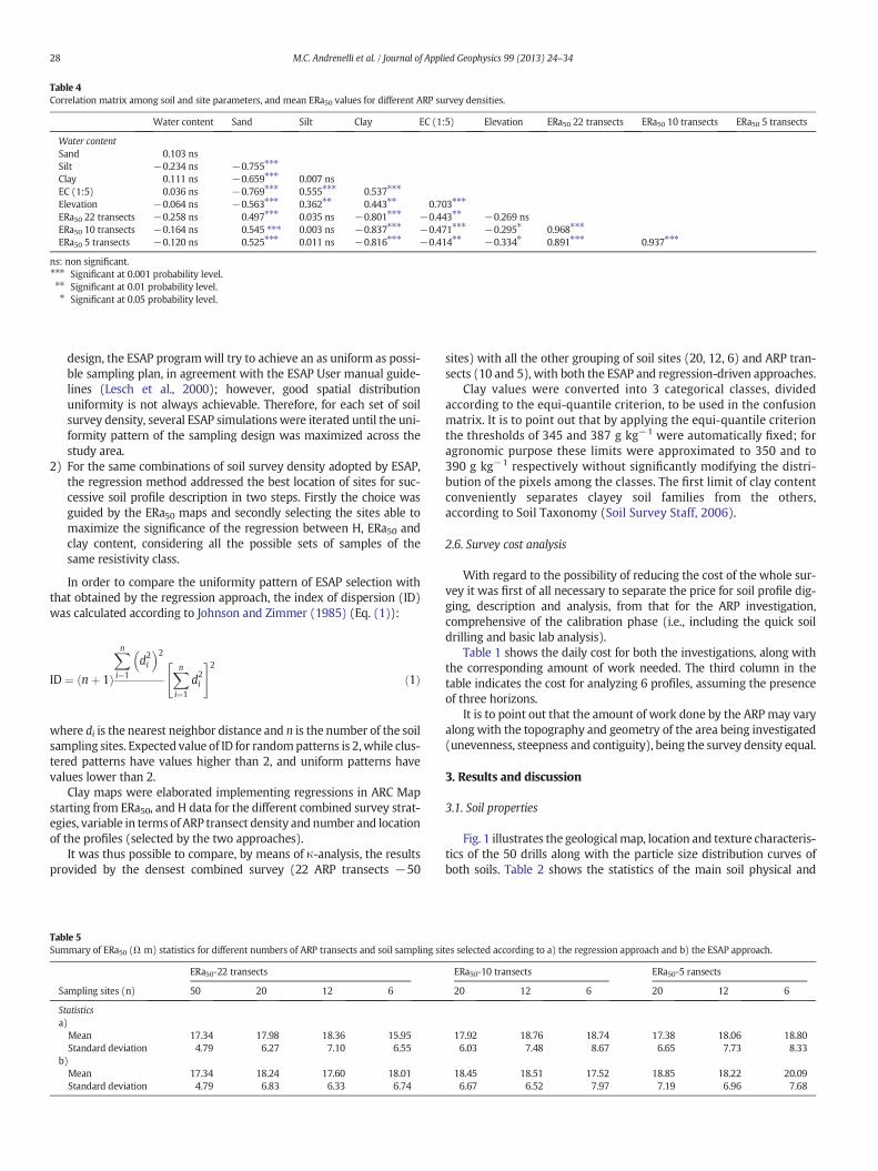
Table 4Correlation matrix among soil and site parameters, and mean ERa50 values for different ARP survey densities.

Water content Sand Silt Clay EC (1:5) Elevation ERa50 22 transects ERa50 10 transects ERa50 5 transects

Water contentSand 0.103 nsSilt −0.234 ns −0.755⁎⁎⁎

Clay 0.111 ns −0.659⁎⁎⁎ 0.007 nsEC (1:5) 0.036 ns −0.769⁎⁎⁎ 0.555⁎⁎⁎ 0.537⁎⁎⁎

Elevation −0.064 ns −0.563⁎⁎⁎ 0.362⁎⁎ 0.443⁎⁎ 0.703⁎⁎⁎

ERa50 22 transects −0.258 ns 0.497⁎⁎⁎ 0.035 ns −0.801⁎⁎⁎ −0.443⁎⁎ −0.269 nsERa50 10 transects −0.164 ns 0.545 ⁎⁎⁎ 0.003 ns −0.837⁎⁎⁎ −0.471⁎⁎⁎ −0.295⁎ 0.968⁎⁎⁎

ERa50 5 transects −0.120 ns 0.525⁎⁎⁎ 0.011 ns −0.816⁎⁎⁎ −0.414⁎⁎ −0.334⁎ 0.891⁎⁎⁎ 0.937⁎⁎⁎

ns: non significant.⁎⁎⁎ Significant at 0.001 probability level.⁎⁎ Significant at 0.01 probability level.⁎ Significant at 0.05 probability level.

28 M.C. Andrenelli et al. / Journal of Applied Geophysics 99 (2013) 24–34

design, the ESAP programwill try to achieve an as uniform as possi-ble sampling plan, in agreement with the ESAP User manual guide-lines (Lesch et al., 2000); however, good spatial distributionuniformity is not always achievable. Therefore, for each set of soilsurvey density, several ESAP simulationswere iterated until the uni-formity pattern of the sampling design was maximized across thestudy area.

2) For the same combinations of soil survey density adopted by ESAP,the regression method addressed the best location of sites for suc-cessive soil profile description in two steps. Firstly the choice wasguided by the ERa50 maps and secondly selecting the sites able tomaximize the significance of the regression between H, ERa50 andclay content, considering all the possible sets of samples of thesame resistivity class.

In order to compare the uniformity pattern of ESAP selection withthat obtained by the regression approach, the index of dispersion (ID)was calculated according to Johnson and Zimmer (1985) (Eq. (1)):

ID ¼ nþ 1ð Þ

Xni¼1

d2i� �2 Xn

i¼1

d2i

" #2

ð1Þ

where di is the nearest neighbor distance and n is the number of the soilsampling sites. Expected value of ID for randompatterns is 2,while clus-tered patterns have values higher than 2, and uniform patterns havevalues lower than 2.

Clay maps were elaborated implementing regressions in ARC Mapstarting from ERa50, and H data for the different combined survey strat-egies, variable in terms of ARP transect density and number and locationof the profiles (selected by the two approaches).

It was thus possible to compare, by means of κ-analysis, the resultsprovided by the densest combined survey (22 ARP transects −50

Table 5Summary of ERa50 (Ω m) statistics for different numbers of ARP transects and soil sampling si

ERa50-22 transects

Sampling sites (n) 50 20 12 6

Statisticsa)

Mean 17.34 17.98 18.36 15.95Standard deviation 4.79 6.27 7.10 6.55

b)Mean 17.34 18.24 17.60 18.01Standard deviation 4.79 6.83 6.33 6.74

sites) with all the other grouping of soil sites (20, 12, 6) and ARP tran-sects (10 and 5), with both the ESAP and regression-driven approaches.

Clay values were converted into 3 categorical classes, dividedaccording to the equi-quantile criterion, to be used in the confusionmatrix. It is to point out that by applying the equi-quantile criterionthe thresholds of 345 and 387 g kg−1 were automatically fixed; foragronomic purpose these limits were approximated to 350 and to390 g kg−1 respectively without significantly modifying the distri-bution of the pixels among the classes. The first limit of clay contentconveniently separates clayey soil families from the others,according to Soil Taxonomy (Soil Survey Staff, 2006).

2.6. Survey cost analysis

With regard to the possibility of reducing the cost of the whole sur-vey it was first of all necessary to separate the price for soil profile dig-ging, description and analysis, from that for the ARP investigation,comprehensive of the calibration phase (i.e., including the quick soildrilling and basic lab analysis).

Table 1 shows the daily cost for both the investigations, along withthe corresponding amount of work needed. The third column in thetable indicates the cost for analyzing 6 profiles, assuming the presenceof three horizons.

It is to point out that the amount of work done by the ARP may varyalong with the topography and geometry of the area being investigated(unevenness, steepness and contiguity), being the survey density equal.

3. Results and discussion

3.1. Soil properties

Fig. 1 illustrates the geologicalmap, location and texture characteris-tics of the 50 drills along with the particle size distribution curves ofboth soils. Table 2 shows the statistics of the main soil physical and

tes selected according to a) the regression approach and b) the ESAP approach.

ERa50-10 transects ERa50-5 ransects

20 12 6 20 12 6

17.92 18.76 18.74 17.38 18.06 18.806.03 7.48 8.67 6.65 7.73 8.33

18.45 18.51 17.52 18.85 18.22 20.096.67 6.52 7.97 7.19 6.96 7.68

Fig. 4. Location of the sampling points for different soil survey strategies according to both the regression driven (above) and the ESAP (below) approaches on ERa50maps for the three ARPdensities investigated.

29M.C. Andrenelli et al. / Journal of Applied Geophysics 99 (2013) 24–34

chemical characteristics indicating that soil EC and sand content arecharacterized by higher variability with respect to the other features.

In relation to the texture analysis, Fig. 1 indicates that on averagethe soil on clays was characterized by lower both median (d50) andmean geometric diameter (dg) compared to the other soil; in addi-tion, the two soils were extremely poorly sorted (high geometricstandard deviation value) and characterized by a symmetricalshape of the granulometric curve; moreover, kurtosis values indicatea platykurtic distribution for clays and a very platykurtic for con-glomerates. The extreme poor sorting of the two soils is responsiblefor the differentiation of the textural classes found within each geol-ogy formation. In particular, on blue clays, the clay textural class rep-resented 50%, whereas the clay–loam textural class represented 33%;the remaining was equally distributed between silt-loam and silty-clay–loam textural classes. On the conglomerates, the clay–loam

textural class dominated (81%) and was followed by clay and loamtextural classes (almost 8% each).

3.2. Resistivity map quality

The interpolation of the ERa50 values using 22, 10, or 5 ARP transectsby means of the Ordinary Kriging procedure produced comparablemaps (Fig. 3). Each density, in spite of the very different numbers ofmeasurements per ha and transect widths, produced similar basic sta-tistics of ERa50 values calculated over the whole area, indicating a highsoil spatial variability (Table 3) in agreement with the textural compo-sition of the soils.

It is noteworthy that only the 10 rows grid, corresponding to a re-duction of almost 40% of both measurements, provided a substantialagreement, in terms of ERa50 predictability, with the result given by

Table 6Coefficient of determination and significance level of the regressions for different numbersof ARP transects and soil sites selected by both the regression and ESAP approaches. IDvalues are also indicated.

ARPtransects(n)

Soil sitenumber (n)

R2 Significancelevel

ID R2 Significancelevel

ID

22 50 0.732 ⁎⁎⁎

Regression approach ESAP selection

22 20 0.830 ⁎⁎⁎ 1.41 0.889 ⁎⁎⁎ 1.2612 0.901 ⁎⁎⁎ 1.42 0.977 ⁎⁎⁎ 1.296 0.989 ⁎⁎ 3.39 0.853 ns 1.46

10 20 0.877 ⁎⁎⁎ 1.41 0.851 ⁎⁎⁎ 1.3312 0.918 ⁎⁎⁎ 2.25 0.890 ⁎⁎⁎ 1.316 0.935 ⁎ 3.13 0.977 ⁎⁎ 1.44

5 20 0.853 ⁎⁎⁎ 4.45 0.889 ⁎⁎⁎ 1.5312 0.906 ⁎⁎⁎ 3.16 0.977 ⁎⁎⁎ 1.266 0.920 ⁎ 3.39 0.853 ns 1.44

ns: non significant.⁎⁎⁎ Significant at 0.001 probability level.⁎⁎ Significant at 0.01 probability level.⁎ Significant at 0.05 probability level.

30 M.C. Andrenelli et al. / Journal of Applied Geophysics 99 (2013) 24–34

the densest ARP survey. In contrast, further reduction to 5 rows reducedsignificantly the ERa50 predictability and produced a moderate agree-ment with the most expensive strategy.

3.3. ARP soil relationships

3.3.1. Correlation matrix between soil properties and resistivity valuesIn order to understand the relationship between ERa50 values and

the soil characteristics, a correlation matrix was produced for thewhole data set— 50 samples (Table 4). Moisture content was not relat-ed to either soil properties or ERa50 values, silt was significantly relatedto ECa andHonly; therefore, these parameters could not be interpolatedover the whole study area starting from the resistivity values. Elevationwas positively linked to clay content in accordance with the differentgeological substratum locations within the vineyard (see Study site de-scription). Table 4 shows as clay percentage assumed the highest corre-lation coefficient versus all ERa50 data (|r| ≥ 0.801) compared to all theother soil properties, and for this reason it was employed to test/com-pare the performance of different soil survey densities.

3.3.2. Resistivity statistics for different sampling site selectionsBefore illustrating the comparison of the clay maps provided by the

two approaches, it is interesting to have a look at themain ERa50 statis-tics for the various survey strategies and site selection approaches(Table 5). Generally, the various selections provided comparable ERa50mean valueswith respect to the densest ARP and soil sampling. Howev-er, as expected, by lowering the number of both ARP transects and soil

Table 7Results of the confusion matrix for the clay accuracy determination on the basis of both the re

22 ARP transects (667 points ha−1)

Soil samples (n) Sample density (n ha−1) ω value κ value Agreement class

Regression approach20 5.71 91% 86% Almost perfect12 3.43 92% 87% Almost perfect6 1.71 76% 63% Substantial

ESAP approach20 5.71 85% 76% Substantial12 3.43 79% 68% Substantial6 –

samples, the discrepancies increased in terms of standard deviationvalues. Fig. 4 indicates, for the three ARP survey densities, the differentselections of soil sampling sites obtained according to the regression(Fig. 4 above) and the ESAP criteria (Fig. 4 below).

3.3.3. Regressions between H–ERa50 data and clay contentAs previously stated, for each sampling site selection strategy, ob-

tained by either the regression or by ESAP approach, regression equa-tions were calculated starting from H and ERa50 data for the varioussoil and ARP survey densities. These equations were then implementedin GIS technologies to map clay content over the study area. The coeffi-cients of determination and the significance levels of the regressions arereported in Table 6, along with the dispersion index (ID) values.

The values in the first row in Table 6 refer to densest combined sur-vey (50 samples — 22 ARP transects) representing the common com-parison term.

It is to point out that the elevation improved the coefficient of deter-mination, for instance from R2 = 0.690 (value not shown) to 0.732 for22 ARP transects combinedwith 50 sites, andmost of all the levels of ac-curacy of clay map over the whole area.

Generally, both approaches provided comparable significant rela-tionships with the exception of the loosest sampling design (6 sitescombined to 22 or 5 ARP transects) where ESAP did not give significantregressions. On the contrary, as expected, ESAP selections gave lower IDvalues providing higher uniformity patterns than regression sites, as il-lustrated in Fig. 4. In particular, for the regression sites only, the reduc-tion of thedensity for both the surveys promoted the clusteringpatternsgeneration (as highlighted by the ID values increase).

Actually, the ESAP procedure minimized the ID, whereas the regres-sions approachmaximized the predictability of clay content. In particu-lar, in the case of the ESAP selection, the regressions which involved 6samples with 22 or 5 ARP transects were not significant (p N 0.05).

Conversely, all the regressions involving at least 12 sites selected bythe regression approachwere highly significant, and only further reduc-tion to 6 sites deteriorated the significance at 0.01 and 0.05 levels, for 22ARP transects and 10 or 5 ARP transects, respectively. Therefore, the re-duction of soil sample number to 1.71 ha−1 affected more the predict-ability of clay than the lowering of the ARP transect number.

3.4. Comparison between regression and ESAP approaches in terms of claypredictability

Table 7 illustrates the accuracy of the clay estimates for the differentsurvey strategies over the study area, provided by the regression andESAP approaches. The results obtained by non significant regressionshave been excluded.

The regression approach provided higher clay predictability thanESAP for the densest ARP survey and loosest soil sampling. Comparableresults are observed with 10 ARP transects. It may be noticed that, as arule, the reduction of the soil sample number affects clay map

gression and ESAP approaches.

10 ARP transects (417 points ha−1) 5 ARP transects (276 points ha−1)

ω value κ value Agreement class ω value κ value Agreement class

83% 73% Substantial 73% 58% Moderate74% 60% Substantial 73% 58% Moderate81% 71% Substantial 72% 57% Moderate

81% 71% Substantial 74% 60% Moderate77% 64% Substantial 74% 60% Moderate80% 69% Substantial –

Fig. 5. Clay maps and corresponding location of the soil sites relative to some convenient combinations of soil and ARP survey densities, all providing at least a substantial agreement.

31M.C. Andrenelli et al. / Journal of Applied Geophysics 99 (2013) 24–34

predictability less than the lowering of the ARP survey intensity, andthat 20 sampling sites are never necessary in all the ARP densities(Table 7), because it is possible to achieve the same accuracy levelwith a lower soil sample number (12 or even 6).

Fig. 5 shows some of the clay maps obtained starting from the re-gression equations listed in Table 5. As a comparison, clay grid valuesprovided by 22 ARP transects and 50 soil samples are also shown. Thelocation of soil sampling sites is also displayed. In particular, as indicatedin Table 6, themap given by 22 transects— 12 sites chosen with regres-sionmethod is more similar to the reference one (almost perfect agree-ment) than the other two maps, providing a substantial accuracy. Thecomparison between the latter two grids outlined that the 6-sites re-gression showed a good reproducibility in the upper part of the map,while 6-site ESAP gave a good similarity in the lower part of the map;in the remaining area the two maps are comparable.

3.5. Comparison of the survey costs

The costs of some possible combinations of survey density (numberof ARP transects and soil sites) are compared in Table 8, along with asketchy description of each activity.

Taking in mind that the ARP employs a day to cover an average sur-face of 15 ha (Table 1), it is possible to hypothesize several alternativesto the densest density, equivalent to 667 points ha−1. The reduction ofthe ARP survey density to 10 or 5 transects (417 or 276 points ha−1)could allow to cover nearly 30 and 60 ha per day, respectively, at thesame cost of 3000EUR (Table 8). In suchhypotheses the number of drills,located according to a regular pattern, required for calibrating the ERa

Table 8The costs of some possible combinations of the survey density.

Area(ha)

Survey density (points/sites ha−1)

Activity

Calibration

ARP survey(EUR)

Drills(n)

Drills(EUR)

Lab(EUR)

15 667/5.71 3000 25 300 75015 667/3.43 3000 25 300 75015 667/1.71 3000 25 300 75030 417/1.71 3000 50 600 150060 276/1.71 3000 100 1200 3000

data, does increase by enlarging the area. In particular, the minimumnumber of drills can be obtained from the maximum values (78 m) ofthe effective range of the semivariograms described in Appendix A.Therefore, supposing a drill every about 6000 m2 (78 × 78 m assumingan omni-directional semivariogram), it is possible to calculate the corre-sponding number for the hectarages indicated in Table 8. The price fordrilling and lab analyses is also indicated in the same table. Going on tothe cost for the soil profile excavation, description and analysis, it is topoint out that, although all the indicated sites are supposed to be exca-vated and observed, the complete description and analysis are typicallyrestricted to one tenth of the profiles, the choice depending on the char-acteristics of the entire soil section.

4. Conclusions

Themost influencing soil characteristics on the resistivity data in thestudy area were the clay content. The relationships we found out be-tween H–ERa50 and clay might be considered constant over time,since themoisture conditions were almost homogeneous and not relat-ed to the resistivity values during the survey.

With respect to the possibility of lowering the survey cost the re-gression procedure offered several possibilities of reducing survey in-tensity with different accuracy levels: if an almost perfect agreementwas required, it would be convenient to dug 3.43 profiles ha−1 incombination with the densest ARP survey. Otherwise, if a substantialagreement might be considered acceptable, even 1.71 profiles ha−1

and 417 ARP points ha−1 would be enough. A moderate agreementmight be achieved with the scarcest combined survey density.

Tot(EUR)

Tot/ha(EUR)

Profiles

Profiles(n)

Escavation(EUR)

Description and analysis(EUR)

85 2677 4283 11,009 73451 1608 2573 8230 54926 802 1283 6134 40951 1603 2565 9268 309

103 3206 5130 12,386 206

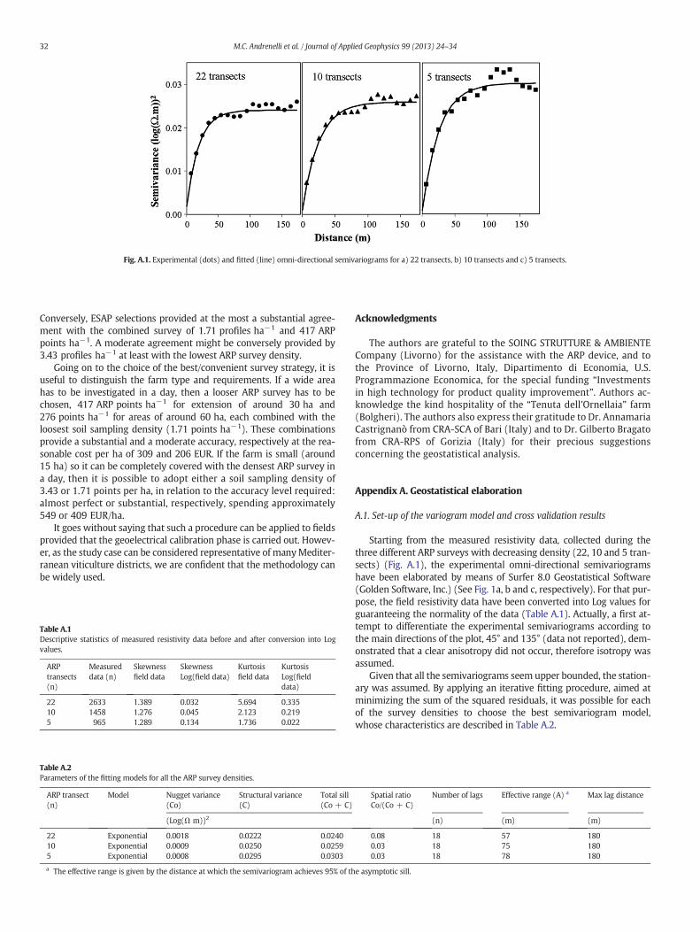
Fig. A.1. Experimental (dots) and fitted (line) omni-directional semivariograms for a) 22 transects, b) 10 transects and c) 5 transects.

32 M.C. Andrenelli et al. / Journal of Applied Geophysics 99 (2013) 24–34

Conversely, ESAP selections provided at the most a substantial agree-ment with the combined survey of 1.71 profiles ha−1 and 417 ARPpoints ha−1. A moderate agreement might be conversely provided by3.43 profiles ha−1 at least with the lowest ARP survey density.

Going on to the choice of the best/convenient survey strategy, it isuseful to distinguish the farm type and requirements. If a wide areahas to be investigated in a day, then a looser ARP survey has to bechosen, 417 ARP points ha−1 for extension of around 30 ha and276 points ha−1 for areas of around 60 ha, each combined with theloosest soil sampling density (1.71 points ha−1). These combinationsprovide a substantial and a moderate accuracy, respectively at the rea-sonable cost per ha of 309 and 206 EUR. If the farm is small (around15 ha) so it can be completely covered with the densest ARP survey ina day, then it is possible to adopt either a soil sampling density of3.43 or 1.71 points per ha, in relation to the accuracy level required:almost perfect or substantial, respectively, spending approximately549 or 409 EUR/ha.

It goes without saying that such a procedure can be applied to fieldsprovided that the geoelectrical calibration phase is carried out. Howev-er, as the study case can be considered representative of manyMediter-ranean viticulture districts, we are confident that the methodology canbe widely used.

Table A.1Descriptive statistics of measured resistivity data before and after conversion into Logvalues.

ARPtransects(n)

Measureddata (n)

Skewnessfield data

SkewnessLog(field data)

Kurtosisfield data

KurtosisLog(fielddata)

22 2633 1.389 0.032 5.694 0.33510 1458 1.276 0.045 2.123 0.2195 965 1.289 0.134 1.736 0.022

Table A.2Parameters of the fitting models for all the ARP survey densities.

ARP transect(n)

Model Nugget variance(Co)

Structural variance(C)

Total sill(Co + C)

(Log(Ω m))2

22 Exponential 0.0018 0.0222 0.024010 Exponential 0.0009 0.0250 0.02595 Exponential 0.0008 0.0295 0.0303

a The effective range is given by the distance at which the semivariogram achieves 95% of th

Acknowledgments

The authors are grateful to the SOING STRUTTURE & AMBIENTECompany (Livorno) for the assistance with the ARP device, and tothe Province of Livorno, Italy, Dipartimento di Economia, U.S.Programmazione Economica, for the special funding “Investmentsin high technology for product quality improvement”. Authors ac-knowledge the kind hospitality of the “Tenuta dell'Ornellaia” farm(Bolgheri). The authors also express their gratitude to Dr. AnnamariaCastrignanò from CRA-SCA of Bari (Italy) and to Dr. Gilberto Bragatofrom CRA-RPS of Gorizia (Italy) for their precious suggestionsconcerning the geostatistical analysis.

Appendix A. Geostatistical elaboration

A.1. Set-up of the variogram model and cross validation results

Starting from the measured resistivity data, collected during thethree different ARP surveys with decreasing density (22, 10 and 5 tran-sects) (Fig. A.1), the experimental omni-directional semivariogramshave been elaborated by means of Surfer 8.0 Geostatistical Software(Golden Software, Inc.) (See Fig. 1a, b and c, respectively). For that pur-pose, the field resistivity data have been converted into Log values forguaranteeing the normality of the data (Table A.1). Actually, a first at-tempt to differentiate the experimental semivariograms according tothe main directions of the plot, 45° and 135° (data not reported), dem-onstrated that a clear anisotropy did not occur, therefore isotropy wasassumed.

Given that all the semivariograms seem upper bounded, the station-ary was assumed. By applying an iterative fitting procedure, aimed atminimizing the sum of the squared residuals, it was possible for eachof the survey densities to choose the best semivariogram model,whose characteristics are described in Table A.2.

Spatial ratioCo/(Co + C)

Number of lags Effective range (A) a Max lag distance

(n) (m) (m)

0.08 18 57 1800.03 18 75 1800.03 18 78 180

e asymptotic sill.

Table A.3Cross-validation results expressed as statistics of the residuals.

ARP transects(n)

MinE MaxE ME RMSE MSE σ2SE αcoefficient

R2

(Ω m)

22 −19.93 15.16 −0.19 2.79 −0.069 1.00 0.97 0.8010 −15.47 10.88 −0.15 2.45 −0.060 1.00 0.98 0.865 −15.59 11.04 −0.16 2.59 −0.061 1.00 0.98 0.88

MinE = Minimum error; MaxE = maximum error; ME = mean error; RMSE = root-mean-square error; MSE = mean of the standardized error; σ2SE = variance of thestandardized error; α is the slope of the regression between measured and predicteddata; R2 is the related coefficient of determination of the regression.

33M.C. Andrenelli et al. / Journal of Applied Geophysics 99 (2013) 24–34

For all the ARP densities the fitted semivariograms were describedby the same combination of the nugget effect plus exponential model,characterized by similar spatial ratio value. This fact indicates that allthe models are affected by a strong spatial dependency while a scarceinfluence of the nugget variance upon the total sill is observed any-where. A certain raise of the nugget value and a decrease of the effectiverange value were also registered by increasing the ARP densities.

In order to evaluate the performance provided by the fitted models,the cross validation procedure was employed. Applied to all the respec-tive data set of points (2633, 1458, and 965 points) and basing on theleave-one-out technique, such a procedure evaluated the residuals (er-rors) along with a detailed statistical summary illustrated in Table A.3.

All the statistical parameters appear quite similar among the ARPsurvey densities, despite a slight deterioration of the performance is ob-served in the densest investigation (lowest coefficient of determinationand highest RMSE value), probably related to the occurrence of someoutliers, not investigated by the other two looser surveys (see bothMinE and MaxE values).

The cross-validation results along with the parameters of the fittingmodels demonstrated that the Ordinary Kriging procedure, adopted tointerpolate the resistivity data, provided comparable accuracy in allthe ARP survey densities. The parameters of the fitting models for thethree ARP survey densities have been successively imported into ARCGIS software to create the related resistivity maps.

Appendix B

B.1. Map accuracy assessment

To compare the results provided by different densities of the ARPand soil survey in terms of ERa50 and clay predictability, the techniqueof the confusion matrix was employed. Such an error matrix compares,on a class-by-class basis, known reference data (ERa50 or Clay class pro-vided by 22 ARP transects and 50 sites) and the corresponding results ofclassification (predicted values) given by the other looser surveys.

In such matrix (n × n) the predicted classification is given as rows,while the reference one (given by 22 ARP transects combined with 50sites) is along the columns. The diagonals represent agreement mapsand the reference data, while the off-diagonal elements represent dif-ferent mis-classifications.

Starting from this table it was possible to calculate themost commonerror estimate, that is the Overall accuracy (ω) given by:

ω ¼Xni¼1

eii�T with T ¼

Xni¼1

XnJ¼1

eij ðB:1Þ

where eii represents the sum of diagonal pixels, eij is the sum of all rowand column elements (T = the total number of the matrix elements)and n the number of categories being considered.

The results were then expressed in terms of κ value, calculatedaccording to the following equation (Landis and Koch, 1977), and agree-ment class.

κ ¼ ϖ−θð Þ= 1−θð Þ ðB:2Þ

where θ is the proportion of pixels which agree exclusively by chance,that in turn is given by:

θ ¼ 1=T2� �Xn

i¼1

eiþeþ j ðB:3Þ

with ei+ and e+j being themarginal total of row i and themarginal totalof column j, respectively and T the total number of the elements of theconfusion matrix.

Therefore, the estimate of κ is the proportion of agreement afterchance is removed from consideration. If all the pixels are in completeagreement then κ is equal to 1; conversely, if there is no agreementamong the pixels (other than what would be expected by chance)then κ is equal to 0. In particular, Landis and Koch (1977) identifiedfive equi-spaced classes of κ values ranging between 0 and 1.0 associat-ed to different agreement classes.

References

Amezketa, E., 2007. Soil salinity assessment using directed soil sampling from a geophys-ical survey with electromagnetic technology: a case study. Span. J. Agric. Res. 5,91–101.

Amezketa, E., de Lersundi, J.D.V., 2008. Soil classification and salinity mapping for deter-mining restoration potential of cropped riparian areas. Land Degrad. Dev. 19,153–164.

Basso, B., Amato, M., Bitella, G., Rossi, R., Kravchenko, A., Sartori, L., Carvahlo, L.M., Gomes,J., 2010. Two-dimensional spatial and temporal variation of soil physical properties intillage systems using electrical resistivity tomography. Agron. J. 102 (2), 440–449.

Bourennane, H., Nicoullaud, B., Couturier, A., King, D., 2004. Exploring the spatial relation-ships between some soil properties and wheat yields in two soil types. Precis. Agric.5, 521–536.

Bramley, R.G.V., 2009. Lessons from nearly 20 years of precision agriculture research, de-velopment, and adoption as a guide to its appropriate application. Crop Pasture Sci.60, 197–217.

Bramley, R.G.V., Lamb, D.W., 2003. Making sense of vineyard variability in Australia. In:Ortega, R., Esser, A. (Eds.), Precision Viticulture. Proceedings of an international sym-posium held as part of the IX Congreso Latinoamericano de Viticultura y Enologia,Chile. Centro de Agricultura de Precisión, Pontificia Universidad Católica de Chile,Facultad de Agronomía e Ingenería Forestal, Santiago, Chile, pp. 35–54.

Bramley, R.G.V., Lamb, D.W., 2006. Precision Viticulture — making sense of vineyard var-iability. Final Report on Project No. CRV99/5 N to the Grape and Wine Research andDevelopment Corporation. Cooperative Research Centre for Viticulture/GWRDC, Ade-laide, Australia.

Bramley, R.G.V., Ouzman, J., Boss, P.K., 2011a. Variation in vine vigour, grape yield andvineyard soils and topography as indicators of variation in the chemical compositionof grapes, wine and wine sensory attributes. Aust. J. Grape Wine Res. 17, 217–219.

Bramley, R.G.V., Trought, M.C.T., Praat, J.P., 2011b. Vineyard variability in Marlborough,New Zealand: characterising variation in vineyard performance and options for theimplementation of Precision Viticulture. Aust. J. Grape Wine Res. 17, 72–78.

Campana, S., Marasco, L., Pecci, A., Barba, L., Dabas, M., Piro, S., Zamuner, D., 2009. Integra-tion of ground remote sensing surveys and archaeological excavation to characterizethe medieval mound (Scarlino,Tuscany, Italy). Archaeol. Prospect. 16, 167–176.

Cassel, F., Goorahoo, S.D., Zoldoske, D., Adhikari, D., 2008. Mapping soil salinity usingground-based electromagnetic induction. In: Metternicht, G., Zinck, A. (Eds.), RemoteSensing of Soil Salinization: Impact on Land Management. CRC Press, Taylor andFrancis Group, Boca Raton, FL, USA, pp. 199–210.

Corwin, D.L., Lesch, S.M., 2003. Application of soil electrical conductivity to precision agri-culture: theory, principles, and guidelines. Agron. J. 95, 455–471.

Corwin, D.L., Lesch, S.M., 2005a. Characterizing soil spatial variability with apparent soilelectrical conductivity I. Survey protocols. Comput. Electron. Agric 46, 103–133.

Corwin, D.L., Lesch, S.M., 2005b. Apparent soil electrical conductivity measurements in ag-riculture. Comput. Electron. Agric. 46, 11–44.

Costantini, E.A.C., Pellegrini, S., Bucelli, P., Barbetti, R., Campagnolo, S., Storchi, P., Magini,S., Perria, R., 2010. Mapping suitability for Sangiovese wine by means of δ13C andgeophysical sensors in soils with moderate salinity. Eur. J. Agron. 33, 208–217.

Dabas, M., 2006. Theory and practice of the new fast electrical imaging system ARP©.Presented at the XV International Summer School in Archaeology, Geophysics forLandscape Archaeology, Grosseto, 10–18 July.

Dabas, M., 2009. Theory and practice of the new fast electrical imaging system ARP©. In:Campana, Piro (Eds.), Seeing the Unseen. Geophysics and Landscape Archaeology.CRC Press, Taylor & Francis Group, London, UK, pp. 105–126.

Dabas, M., Hesse, A., Tabbagh, J., 2000. Experimental resistivity survey atWroxeter archae-ological site with a fast and light recording device. Archaeol. Prospect. 7, 107–118.

FAO, 1979. Soil survey investigations for irrigation. FAO Soils Bulletin No. 42.FAO, Rome(188 p.).

FAO-ISRIC-IUSS, 2006. World reference base for soil resources. A Framework for Interna-tional Classification, Correlation and Communication. World Soil Resources Report,106. Food and Agriculture Organization, Rome, Italy.

Farahani, H.J., Flynn, R.L., 2007. Map quality and zone delineation as affected by width ofparallel swaths of mobile agricultural sensors. Biosyst. Eng. 96 (2), 151–159.

34 M.C. Andrenelli et al. / Journal of Applied Geophysics 99 (2013) 24–34

Frogbrook, Z.L., Oliver, M.A., 2000. The effects of sampling on the accuracy of predictionsof soils properties for precision agriculture. In: Heuvelink, G.B.M., Lemmens, M.J.M.(Eds.), Accuracy 2000. Proceedings of the 4th international symposium on spatial ac-curacy assessment in natural resources and environmental sciences. Delft: Delft Uni-versity Press, The Netherlands, pp. 225–232.

Frogbrook, Z.L., Oliver, M.A., 2007. Identifying management zones in agricultural fieldsusing spatially constrained classification of soil and ancillary data. Soil Use Manag.23 (1), 40–51.

I numeri del vino, 2008. http://www.inumeridelvino.it/2008/03/la-dimensione-delle-aziende-vinicole-in-europa-dati-1990–2003.html (verified 2012 July 17th).

Iqbal, J., Thomasson, J.A., Jenkins, N.J., Owens, R.P., Whisler, D.F., 2005. Spatial variabilityanalysis of soil physical properties of alluvial soils. Soil Sci. Soc. Am. J. 69, 1338–1350.

ISTAT, 2010. http://www3.istat.it/salastampa/comunicati/non_calendario/20110705_00/(verified 2012 July 17th).

Johnson, R.B., Zimmer, W.J., 1985. A more powerful test for dispersion using distancemeasurements. Ecology 66, 1669–1675.

Johnson, C.K., Doran, J., Duke, H.R., Wienhold, B.J., Eskridge, K., Shanahan, J.F., 2001. Fieldscale electrical conductivity mapping for delineating soil condition. Soil Sci. Soc. Am. J.65 (6), 1829–1837.

Landis, J.R., Koch, G.G., 1977. The measurement of observer agreement for categoricaldata. Biometrics 33, 159–174.

Lesch, S.M., Rhoades, J.D., Corwin, D.L., 2000. ESAP-95 version 2.01R: user manual and tu-torial guide. In: Brown Jr., George E. (Ed.), Research Rpt. USDA-ARS, 146. Salinity Lab-oratory, Riverside, CA, USA.

Morari, F., Castrignanò, A., Pagliarin, C., 2009. Application of multivariate geostatistics indelineating management zones within a gravelly vineyard using geo-electrical sen-sors. Comput. Electron. Agric. 68, 97–107.

Oline, D.K., Grant, M.C., 2002. Scaling patterns of biomass and soil properties: an empiricalanalysis. Landsc. Ecol. 17, 13–26.

Oliver, M.A., Frogbrook, Z.L., 1998. Sampling to estimate soil nutrients for precision agri-culture. Proceedings of the International Fertiliser Society, No. 417.

Ortega, R., Esser, A., Santibañez, O., 2003. Spatial variability of wine grape yield and qual-ity in Chilean vineyards: economic and environmental impacts. In: Stafford, J.,Werner, A. (Eds.), Precision Agriculture, Proceedings of the 4th European Conferenceon Precision Agriculture. Wageningen Academic Publishers, The Netherlands,pp. 499–506.

Rossi, R., Pollice, A., Diago, M.P., Oliveira, M., Millan, B., Bitella, G., Amato, M., Tardaguila, J.,2013. Using an automatic resistivity profiler soil sensor on-the-go in precision viticul-ture. Sensors 13, 1121–1136.

Samouelian, A., Cousin, I., Tabbagh, A., Bruand, A., Richard, G., 2005. Electrical resistivitysurvey in soil science: a review. Soil Tillage Res. 83 (2), 173–193.

Sobieraj, J.A., Elsenbeer, H., Cameron, G., 2004. Scale dependency in spatial patterns of sat-urated hydraulic conductivity. Catena 55, 49–77.

Soil Survey Staff, 2006. Keys to Soil Taxonomy, 10th ed. USDA, Natural Resources Conser-vation Service, NY, USA.

Western, A.W., Blöschl, G., 1999. On the spatial scaling of soil moisture. J. Hydrol. 217,203–224.

Wienhold, B.J., Doran, J.W., 2008. Apparent electrical conductivity for delineatingspatial variabilities in soil properties. In: Allred, B.J., et al. (Ed.), Handbook ofagricultural geophysics (211–215). CRC Press, Taylor and Francis Group, BocaRaton, FL, USA.

Wu, S.D., Usery, E.L., Finn, M.P., Bosch, D., 2009. Effects of sampling interval on spatial pat-terns and statistics of watershed nitrogen concentration. GIScience Remote Sens. 46(2), 172–186.