Journal of Applied Geophysics 123 (2015) 81–92

Contents lists available at ScienceDirect

Journal of Applied Geophysics

j ourna l homepage: www.e lsev ie r .com/ locate / j appgeo

Mapping localised freshwater anomalies in the brackish paleo-lakesediments of the Machile–Zambezi Basin with transient electromagneticsounding, geoelectrical imaging and induced polarisation

Mkhuzo Chongo a,⁎, Anders Vest Christiansen b, Gianluca Fiandaca b, Imasiku A. Nyambe c,Flemming Larsen d, Peter Bauer-Gottwein a

a Technical University of Denmark, Department of Environmental Engineering, Miljøvej, Building 113, 2800 Kgs, Lyngby, Denmarkb Aarhus University, Department of Geoscience, C.F. Møllers Alle 4, 8000-Århus C, Denmarkc University of Zambia, School of Mines, Department of Geology, Great East Road Campus, P.O. Box 32379, Lusaka, Zambiad Geological Survey of Denmark and Greenland (GEUS), Geochemistry, Øster Volgade 10, 1350 København K, Denmark

⁎ Corresponding.E-mail address: mkhuc@env.dtu.dk (M. Chongo).

http://dx.doi.org/10.1016/j.jappgeo.2015.10.0020926-9851/© 2015 Elsevier B.V. All rights reserved.

a b s t r a c t

a r t i c l e i n f o

Article history:Received 21 January 2015Received in revised form 4 October 2015Accepted 6 October 2015Available online 9 October 2015

Keywords:TEMDCIPJoint inversionSurface water/groundwater interactionZambezi RiverZambia

A recent airborne TEM survey in theMachile–Zambezi Basin of southwestern Zambia revealed high electrical re-sistivity anomalies (around 100 Ωm) in a low electrical resistivity (below 13 Ωm) background. The near surface(0–40m depth range) electrical resistivity distribution of these anomalies appeared to be coincident with super-ficial features related to surfacewater such as alluvial fans andflood plains. This paper describes the application oftransient electromagnetic soundings (TEM) and continuous vertical electrical sounding (CVES) using geo-electrics and time domain induced polarisation to evaluate a freshwater lens across a flood plain on the northernbank of the Zambezi River at Kasaya in south western Zambia. Coincident TEM and CVES measurements wereconducted across the Simalaha Plain from the edge of the Zambezi River up to 6.6 km inland. The resultingTEM, direct current and induced polarisation data sets were inverted using a new mutually and laterallyconstrained joint inversion scheme. The resulting inverse model sections depict a freshwater lens sitting ontop of a regional saline aquifer. The fresh water lens is about 60 m thick at the boundary with the ZambeziRiver and gradually thins out and deteriorates inwater quality further inland. It is postulated that the freshwaterlens originated as a result of interaction between the Zambezi River and the salty aquifer in a setting in whichevapotranspiration is the net climatic stress. Similar high electrical resistivity bodies were also associated withother surface water features located in the airborne surveyed area.

© 2015 Elsevier B.V. All rights reserved.

1. Introduction

The interaction between surface water and groundwater has beenstudied extensively around the world (Milosevic et al., 2012;Shanafield and Cook, 2014; Sophocleous, 2002; Westbrook et al.,2005; Winter, 1999; Zarroca et al., 2015; Zhou et al., 2014) using differ-ent approaches, and increasingly geophysical methods are being incor-porated into such studies.

Specific examples of studies that have used geophysical data to in-vestigate hydrogeological phenomenon include Bauer et al. (2006)who described the process of salt accumulation on islands within theOkavango Delta, related to the interaction between surface water andgroundwater under evapo-concentration using a combination of elec-trical resistivity tomography (ERT) (which is the same as CVES with re-spect to geo-electrics) and hydrodynamic modeling; Sonkamble et al.(2014) who evaluated the extent of aquifer pollution from industrial

effluent across the flood plain of the Palar River at Ambur Town(India) using 1D and 2D geo-electrics correlated with in-situ waterquality data and ground penetrating radar; Shalem et al. (2014) whostudied the interaction of the Alexander River with groundwater as itcuts its way across a mostly sandy Quaternary coastal aquifer on theeastern coast of the Mediterranean Sea; and Zarroca et al. (2014) whoevaluated coastal discharge processes at the Peníscola marsh on theSpanish Mediterranean coast using electrical resistivity imaging andtemperature, salinity and 224Ra, 222Rn tracer tests coupled withpetrophysical analysis.

Thus geophysical techniques such as ERT are well suited for gather-ing data at high spatial resolution in comparison to for example pointmeasurements of hydrogeological parameters at sparsely spaced bore-holes (Zarroca et al., 2014). An overall assessment strategy using a com-bination of different geophysical methods and traditionalhydrogeological methods can therefore be advantageous (Brodie et al.,2007; Rubin and Hubbard, 2006). In this regard, TEM (Danielsen et al.,2003; Harthill, 1976; Nabighian, 1991; Xue et al., 2012), direct currentgeo-electrics (DC) (Aizebeokhai, 2010; Dahlin, 2001; Loke, 1999; Loke

82 M. Chongo et al. / Journal of Applied Geophysics 123 (2015) 81–92

et al., 2013) and induced polarisation (IP) (Bertin and Loeb, 1969;Dahlin et al., 2002; Fiandaca et al., 2012; Fiandaca et al., 2013; Titovet al., 2002) techniques are quite suitable for environmental andhydro-geological investigations particularly in sedimentary terrain.

Traditionally, TEM, DC and IP techniques have been deployed sepa-rately even for investigations at the same study site (Bauer et al.,2006; Ezersky et al., 2011; Guerin et al., 2001; Nassir et al., 2000;Vaudelet et al., 2011) although it is now common to have instrumenta-tion that measures both DC and IP in the same field setup (Aristodemouand Thomas-Betts, 2000; Marescot et al., 2008). As a result, differenttypes of data sets are quite often generated for the same physical or en-vironmental phenomenon by inverting each type of data set individual-ly. Nevertheless, major benefits can be derived from joint inversion ofdifferent types of data that observe the same phenomenon and canlead to more accurate interpretations. Thus many studies have success-fully used one form of joint inversion or another such as DC-TEM(Albouy et al., 2001; Christiansen et al., 2007; Danielsen et al., 2007)and MRS-TEM (Behroozmand et al., 2012; Vilhelmsen et al., 2014).Examples of DCIP joint inversions are scarce in the literature with thenormal practice being to independently invert the DC and IP data eitheras separate inversion jobs or in one inversion job but without any of thedata sets influencing the other during the inversion process. Further-more, joint DCIP–TEM inversions have not been reported in the litera-ture before. This paper therefore presents a first case study of jointinversion of DCIP–TEM data.

The focus of this paper is on local scale electrical resistivity anoma-lies derived from interpreting regional scale airborne TEM data interms of surface water/groundwater interaction in theMachile–Zambe-zi Basin. The objectives were to describe the occurrence of high electri-cal resistivity anomalies in the low electrical resistivity backgroundenvironment of the Machile–Zambezi Basin; conduct local scale TEMand direct current-induced polarisation (DCIP) CVES measurementsalong a transect cutting across an area exhibiting electrical resistivity

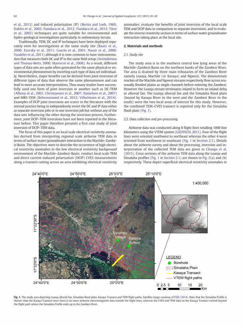
Fig. 1. The study area depicting Loanja alluvial fan, Simalaha flood plain, Kasaya Transect and Tshorter than the Kasaya Transect since there is no more airborne electromagnetic data outsidthe flight path where the Simalaha Profile ends up to the Zambezi River.

anomalies; evaluate the benefits of joint inversion of the local scaleTEM and DCIP data in comparison to separate inversions; and to evalu-ate the inverse resistivity section in terms of surfacewater groundwaterinteraction taking place at the local site.

2. Materials and methods

2.1. Study site

The study area is in the southern central low lying areas of theMachile–Zambezi Basin on the northern banks of the Zambezi River.The area is drained by three main tributaries of the Zambezi Rivernamely Loanja, Machile (or Kasaya) and Ngwezi. The downstreamreaches of theMachile andNgwezi streams respectivelyflowacross sea-sonally flooded plains as single channels before entering the Zambezi.However the Loanja stream terminates inland to form an inland deltaor alluvial fan. The Loanja alluvial fan and the Simalaha flood plain(bound by Kasaya River to the west and the Zambezi River to thesouth) were the two local areas of interest for this study. However,the combined TEM–CVES transect is reported only for the Simalahaflood plain (Fig. 1).

2.2. Data collection and pre-processing

Airborne data was conducted along 8 flight lines totalling 1000 linekilometers using the VTEM system (GEOTECH, 2011). Four of the flightlines were oriented southwest to northeast whereas the other 4 wereoriented from northwest to southeast (Fig. 1 in Section 2.1). Detailsabout the airborne survey and about the processing, inversion and in-terpretation of the collected TEM data are given in Chongo et al.(2015). Cross sections of the airborne TEM data along the Loanja andSimalaha profiles (Fig. 1 in Section 2.1) are shown in Fig. 2(a) and (b)respectively. These depict superficial electrical resistivity anomalies in

EM flight paths. Satellite image courtesy of ESRI (2014). Note that the Simalaha Profile ise the flight lines, whereas the CVES and TEM data on the Kasaya Transect extend beyond

Fig. 2. (a) Electrical resistivity cross section along Loanja Profile (Fig. 1 in Section 2.1) from the airborne transient electromagnetic data. (b) Interpolated electrical resistivity cross sectionalong Simalaha Profile (Fig. 1 in Section 2.1) from the airborne TEM data. Note that Loanja and Simalaha profiles are not drawn to scale nor are they the same length since Loanja Profile(about 106 km long) is along a flight line whereas Simalaha Profile (about 5.7 km long) cuts across flight lines and as a result has a more limited data extent.

83M. Chongo et al. / Journal of Applied Geophysics 123 (2015) 81–92

an otherwise low electrical resistivity background (saline environment)and were the basis of the detailed local scale study conducted on theKasaya transect presented in this paper.

The detailed local scale geophysical investigation conducted acrossthe Simalaha Plain at Kasaya (Fig. 1 in Section 2.1) comprised thefollowing:

i. 6.6 km of CVES (Loke, 1999; Loke et al., 2013; Nassir et al., 2000)measurements at 5 m electrode spacing using the gradient array(Dahlin and Zhou, 2006) with 25,003 data points. The TerrameterLS (ABEM(a), 2012) was used for the CVES to measure both direct

Fig. 3. (a) Terrameter LS transmitter current and voltagewaveforms and input voltages fromvarcurves from the various channels of the Terrameter LS measured during transmitter current of

current electrical resistivity (DC) (Loke et al., 2013) and time domaininduced polarisation (IP) (Johnson, 1984) hence the term DCIP todenote the combination of DC and IP measurements in a roll-alongsetup (information on the transmitter and receiver characteristicsof the Terrameter LS is given in Section 2.3 below); and

ii. Sixty-four single site TEM (Christiansen et al., 2006) soundings usingthe Aarhus University/ABEM WalkTEM system; and another set of64 central loop TEM soundings using the Geonics ProTEM 47D in-strument (Geonics, 2006) at the same positions as the WalkTEMsoundings. Thus the total number of TEM soundings along the

ious input channels based on the 4 electrode configuration. (b) Induced polarisation decayf time.

Fig. 4. (a) WalkTEM transmitter waveform and (b) typical earth response.

84 M. Chongo et al. / Journal of Applied Geophysics 123 (2015) 81–92

transect line was 128 spaced at approximately 100 m along the 6.6km transect line per pair ofWalkTEM/ProTEM47D soundings (infor-mation on the transmitter and receiver characteristics of theWalkTEM is given in Section 2.3 below). However data from theProTEM instrument was not used for this paper.

The DCIP data was pre-processed by removing all data points withnegative electrical resistivity and data variations greater than 1.5%. Thedata that was removed this way represented only 3.3% of the original

Fig. 5. (a) Illustration of the variation of thepetro-physical relation (Eq. 1) for different parameteis the curvefitting themeasured boreholefluid conductivity at Kasaya and the unsaturated formwith depth from an induction log and TEM sounding at Kasaya School in Machile–Zambezi Bas

data — i.e. 851 filtered out measurements from a total of 25,857 DCIPmeasurements. The data set was then imported into the Aarhus Work-bench with the IP data gated into 10 channels. Data processing in theWorkbench comprised semi-automatic removal of bad IP data by settinga maximum slope change for the IP decay curves followed by visual in-spection of theDCand IPdata points along theprofile and consequent dis-abling of the outliers. The DCIP noise model was set to 1.03 uniformstandard deviation (USTD) on DC and 1.15 USTD on IP whereas thethreshold on voltage was set to 2.0 mV. For the WalkTEM data we useddata from 77.6 μs to 2.84 ms, focusing on the deep information only.

rs (porosity (ϕ), volumeticwater content exponent (u) and clay content (C)). Kasaya curveation resistivitymeasuredby TEMat the same location. (b) Variation of electrical resistivityin.

85M. Chongo et al. / Journal of Applied Geophysics 123 (2015) 81–92

2.3. Instrumentation

As mentioned above, the geophysical equipment used for this papercomprised the Terrameter LS for geo-electric measurenments and theWalkTEM for transient electromagnetic measurenments. Waveformcharacteristics for the Terrameter LS (ABEM(a), 2012) and theWalkTEM (ABEM(b), 2014) are outlined below in sections 2.3.1 and2.3.2 respectively.

2.3.1. Terrameter LS waveform characteristicsThe transmitter waveform of the Terrameter LS was in the form of a

square wave and comprised a positive and a negative pulse as shown inFig. 3. The period of the transmitter waveformwas automatically deter-mined by the Terrameter LS to be 6.15 s taking into account the powerline frequency of 50 Hz and DC delay and acquisition times of 0.4 s and0.6 s respectively and the time needed to perform the chargeabilitymeasurenments. Thus the transmitter waveform was characterised bya 1 s positive pulse, followed by an off time of 1.77 s and then a negativepulse also of 1 s duration followed by an off time of 2.38 s. IPmeasurenments were performed during both off times. Self-potential

Fig. 6. Inverse electrical resistivity cross sections and residual plots. (a)–(b), Inverse electrical restrical resistivity cross section and residual plot respectively for LCI of TEM data; and (e)–(f), invinversion) of DC and TEM data. On the residual plots, blue lines are for DC residuals whereas g

measurenments on the other handwere conducted only during the sec-ond off time hence its longer duration. Eachmeasurement comprised atleast two cycles so thatmeasured voltages could be averaged in order toeliminate zero shift and linear drift during the measurement cycle(ABEM(a), 2012). Furthermore, the shape of the transmitter waveformprevented polarisation from occurring at the electrodes in addition toremoving any background voltage or self-potential (Binley andKemna, 2006).

The Terrameter LS is amultichannel auto switching instrumentwhichwhen compared to instruments with separate transmitter/receiver unitshas low power, voltage and current ratings of not more than 250 W,1000 V and 3 A respectively. This is in contrast to the 3000 V/10 A reach-able with separate transmitter/receiver instruments. However,multichannel auto switching instruments allow for more freedom inthe array selection for using arrays with small geometrical factor values(e.g. the gradient array) in comparison with instruments with separatetransmitter/receiver units (i.e. the dipole-dipole configuration). The lowgeometrical factor values imply higher IP voltages sampled by the instru-mentswhich partly compensates for the smaller injected current (Gazotyet al., 2013). In addition, processing of the full-decay IP data (as was the

istivity cross section and residual plot respectively for LCI of DC data; (c)–(d), inverse elec-erse electrical resistivity cross section and residual plot respectively for MCI-LCI (i.e. jointreen lines are for TEM residuals.

86 M. Chongo et al. / Journal of Applied Geophysics 123 (2015) 81–92

case for this paper) allows for the effective deletion of spurious decayssuch that in the end there is reliable data with multichannel auto-switching instruments also in addition to tomographic coverage.

2.3.2. WalkTEM waveform characteristicsThe WalkTEM instrument utilises a short duration (about 10 ms)

current pulse to induce eddy currents into the subsurface which inturn generate secondary electromagnetic fields that can be detectedby a receiver coil placed at the surface (ABEM(b), 2014; Christiansenet al., 2006; Nabighian, 1991). Characteristic waveforms and earth re-sponses for a TEM sounding depicting the low moment and high mo-ment curves are shown in Fig. 4. The low moment is designedobtaining information about the conductivity structure of the shallowsubsurface whereas the high moment provides information about theconductivity structure of the deeper subsurface.

2.4. Inversion methodology

DC and TEM data were inverted separately using the 1D laterallyconstrained inversion (LCI) (Auken et al., 2005) scheme. Subsequently,a joint inversion using the mutually and laterally constrained inversionscheme of Christiansen et al. (2007) was conducted on the DC and TEMdata as a single inversion. This was then extended to include IP datausing the Cole–Cole model setup (Fiandaca et al., 2012; Gazoty et al.,2012b) so that the final inversion was a joint inversion of DCIP andTEM data. Thus the DCIP and TEM model parameters being modeledcomprised (intrinsic chargeability (M0), frequency dependence con-stant (c), time constant (τ), formation electrical resistivity (ρ) andlayer thicknesses). The inversion algorithm AarhusInv (Auken et al.,2014) was used for all inversions presented in this paper.

Asmentioned in Section 2.2, the interval of TEM soundings along theKasaya transect was approximately every 100 mwhereas the DCIP datawas collectedwith 5mgradient array electrode spacing. The lateral con-straints on the TEM models were setup such that each TEM model wasconstrained only to the adjacent TEM model on either side along thetransect line. Similarly, eachDCIPmodel was constrained only to the ad-jacent DCIP models. Treatment of mutual TEM–DCIP constraints is ex-plained below.

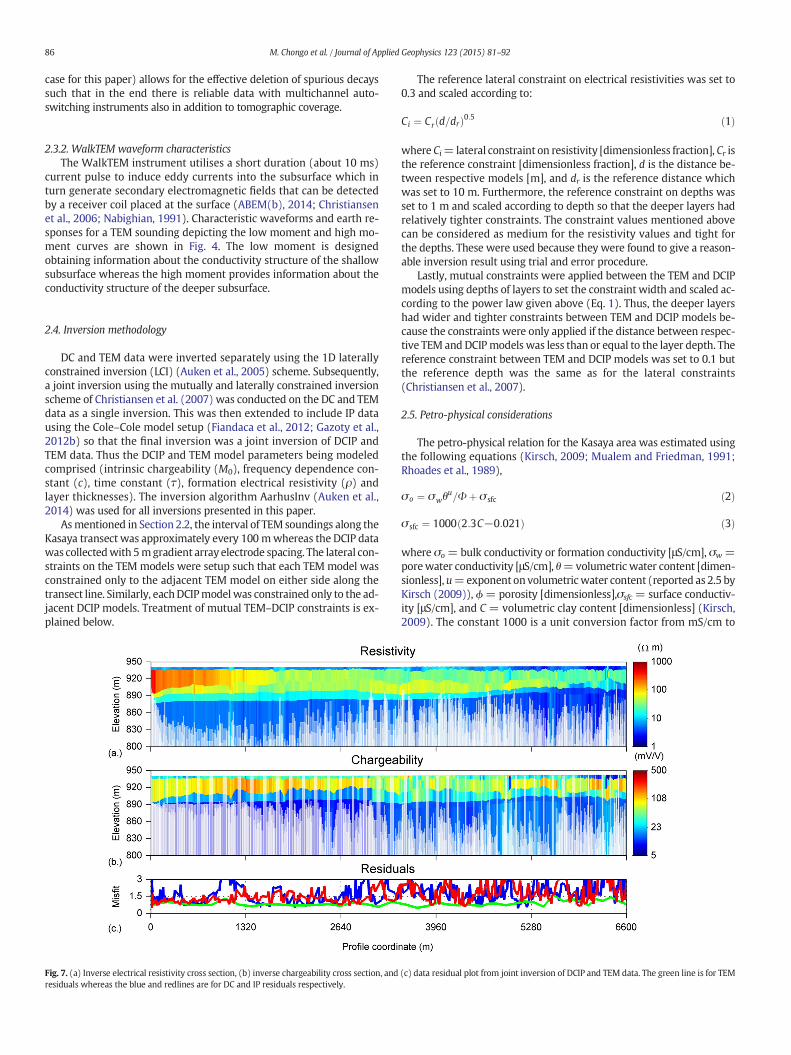
Fig. 7. (a) Inverse electrical resistivity cross section, (b) inverse chargeability cross section, andresiduals whereas the blue and redlines are for DC and IP residuals respectively.

The reference lateral constraint on electrical resistivities was set to0.3 and scaled according to:

Ci ¼ Cr d=drð Þ0:5 ð1Þ

where Ci=lateral constraint on resistivity [dimensionless fraction], Cr isthe reference constraint [dimensionless fraction], d is the distance be-tween respective models [m], and dr is the reference distance whichwas set to 10 m. Furthermore, the reference constraint on depths wasset to 1 m and scaled according to depth so that the deeper layers hadrelatively tighter constraints. The constraint values mentioned abovecan be considered as medium for the resistivity values and tight forthe depths. These were used because they were found to give a reason-able inversion result using trial and error procedure.

Lastly, mutual constraints were applied between the TEM and DCIPmodels using depths of layers to set the constraint width and scaled ac-cording to the power law given above (Eq. 1). Thus, the deeper layershad wider and tighter constraints between TEM and DCIP models be-cause the constraints were only applied if the distance between respec-tive TEM and DCIPmodels was less than or equal to the layer depth. Thereference constraint between TEM and DCIP models was set to 0.1 butthe reference depth was the same as for the lateral constraints(Christiansen et al., 2007).

2.5. Petro-physical considerations

The petro-physical relation for the Kasaya area was estimated usingthe following equations (Kirsch, 2009; Mualem and Friedman, 1991;Rhoades et al., 1989),

σo ¼ σwθu=Φþ σ sfc ð2Þ

σ sfc ¼ 1000 2:3C−0:021ð Þ ð3Þ

where σo = bulk conductivity or formation conductivity [μS/cm], σw =porewater conductivity [μS/cm], θ=volumetric water content [dimen-sionless],u=exponent on volumetricwater content (reported as 2.5 byKirsch (2009)), ϕ = porosity [dimensionless],σsfc = surface conductiv-ity [μS/cm], and C = volumetric clay content [dimensionless] (Kirsch,2009). The constant 1000 is a unit conversion factor from mS/cm to

(c) data residual plot from joint inversion of DCIP and TEM data. The green line is for TEM

87M. Chongo et al. / Journal of Applied Geophysics 123 (2015) 81–92

μS/cm whereas the constants 2.3 and 0.021 are empirical factors as de-rived by Rhoades et al. (1989).

For fully saturated conditions applicable to groundwater, the volu-metric water content was taken to be the same as the porosity meaningthat Eq. 2 could be simplified as:

σo ¼ σwФv þ σ sfc ð4Þ

where the porosity exponent,

v ¼ u−1: ð5Þ

The various parameters of Eqs. 2 and 3 (porosity, porosity exponentand clay content) were adjusted in order to obtain the best curve fittingthrough the Kasaya pore water point and the unsaturated formation

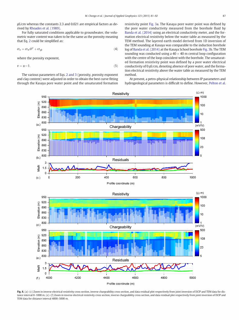
Fig. 8. (a)–(c) Zoom in inverse electrical resistivity cross section, inverse chargeability cross sectance interval 0–1000m. (e)–(f) Zoom in inverse electrical resistivity cross section, inverse charTEM data for distance interval 4000–5000 m.

resistivity point Fig. 3a. The Kasaya pore water point was defined bythe pore water conductivity measured from the borehole fluid byBanda et al. (2014) using an electrical conductivity meter, and the for-mation electrical resistivity below the water table as measured by theTEM method. The layered earth model derived from 1D inversion ofthe TEM sounding at Kasaya was comparable to the induction boreholelog of Banda et al. (2014) at the Kasaya School borehole Fig. 3b. The TEMsounding was conducted using a 40 × 40 m central loop configurationwith the centre of the loop coincidentwith the borehole. The unsaturat-ed formation resistivity point was defined by a pore water electricalconductivity of 0 μS/cm, denoting absence of porewater, and the forma-tion electrical resistivity above the water table as measured by the TEMmethod.

At present, a petro-physical relationship between IP parameters andhydrogeological parameters is difficult to define. However, Pelton et al.

tion, and data residual plot respectively from joint inversion of DCIP and TEM data for dis-geability cross section, and data residual plot respectively from joint inversion of DCIP and

88 M. Chongo et al. / Journal of Applied Geophysics 123 (2015) 81–92

(1978) observed that chargeability (Cole–Cole parameterM0) and timeconstant (Cole–Cole parameter τ) were directly proportional to fluidconcentration and that grain sizewas inversely proportional and direct-ly proportional toM0 and τ respectively. On the other hand, Slater andLesmes (2002) using an experimental laboratory freshwater intrusioninto salty water model observed that the chargeability was directly pro-portional to the fluid resistivity— i.e. inversely proportional to the fluidconductivity in contrast to observations by Pelton et al. (1978). Further-more, Slater and Lesmes (2002) could not find any clear correlation be-tween chargeability and clay content for various mixtures of sand andbentonite clay. However, a correlation was found to exist betweenclay content and the product of fluid conductivity and chargeability.

Given the observations by Slater and Lesmes (2002), the petro-physical relation given by Eq. (2) is assumed to hold for this study,given that the electrical resistivity models produced from the jointDCIP–TEM inversion are informed or constrained by the chargeabilitymodels. Further research is required for better treatment of IP parame-ters with respect to hydrogeological considerations (Gazoty et al.,2012a; Gazoty et al., 2012b; Weller et al., 2013).

2.6. Depth of investigation

The depth of investigation (DOI) (Christiansen and Auken, 2012;Oldenburg and Li, 1999; Roy and Apparao, 1971; Spies, 1989) can beused as a way of evaluating the degree to which measured data andtheir associated uncertainty or noise level are able to resolve the param-eters of an inverse layered earthmodel (Christiansen and Auken, 2012).In this paper, DOI estimation was based on recalculation of the Jacobianmatrix of the final 1D inverse model, taking into account the full systemtransfer function, system geometry, the data and the noise level on thedata (Christiansen and Auken, 2012), but not taking into account inthe computation the model regularisation. From the Jacobian matrix,cumulated sensitivities were computed from which the DOI wasdeduced based on an empirical cumulative sensitivity threshold valueor global threshold (Christiansen and Auken, 2012). Two global thresh-old values were used in this paper: 0.75, for deeper estimation of DOI(or lower DOI) and 1.5, for shallower estimation of DOI (or upperDOI). It should be noted that different DOIs will result for inversemodels from different data types based on the same global thresholdbecause the sensitivities of the different data types do not behave in ex-actly the same way. For example, DC data have higher sensitivities for

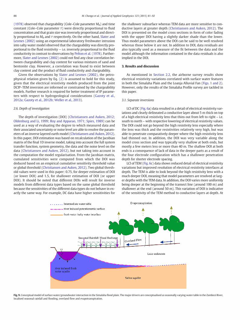
Fig. 9.Conceptualmodel of surfacewater/groundwater interaction in the Simalaha flood plain. Tlocalised seasonal rainfall and flooding, overland flow and evapotranspiration.

the shallower subsurface whereas TEM data are more sensitive to con-ductive layers at greater depth (Christiansen and Auken, 2012). TheDOI is presented on the model cross sections in form of color fadingwith the upper DOI having a slightly darker shade than the lower.Thus model parameters above the DOI can be said to be well resolvedwhereas those below it are not. In addition to DOI, data residuals arealso typically used as a measure of the fit between the data and themodel although the information contained in the data residuals is alsoimplied in the DOI.

3. Results and discussion

As mentioned in Section 2.2, the airborne survey results showelectrical resistivity variations correlated with surface water featuresin both the Simalaha Plain and the Loanja Alluvial Fan (Figs. 1 and 2).However, only the results of the Simalaha Profile survey are tackled inthis paper.

3.1. Separate inversions

LCI of DC (Fig. 6a) data resulted in a detail of electrical resistivity var-iations and clearly delineated a conductive layer about 5 m thick on topof a high electrical resistivity lens that thins out from left to right – i.e.south to north –with respective lowering of electrical resistivity values.The DOI could not go beyond the high resistivity lens especially wherethe lens was thick and the resistivities relatively very high, but wasable to penetrate comparatively deeper where the high resistivity lenshad thinned out. In addition, the DOI was very variable along themodel cross section and was typically very shallow at both ends, butmostly a few meters less or more than 40 m. The shallow DOI at bothends is a consequence of lack of data in the deeper parts as a result ofthe four electrode configuration which has a shallower penetrationdepth for shorter electrode spacing.

LCI of TEM (Fig. 6c) data shows reduced detail of electrical resistivityvariations but improved resolution of electrical resistivity interfaces atdepth. The TEM is able to look beyond the high resistivity lens with amuch deeper DOI, meaning that model parameters are resolved at larg-er depthswith the TEM data. In addition, the DOI variesmore uniformlybeing deeper at the beginning of the transect line (around 100 m) andshallower at the end (around 50 m). This variation of DOI is indicativeof the sensitivity of the TEM method to conductive layers at depth. At

hemajor drivers are conceptualised as seasonally varyingwater table in the Zambezi River,

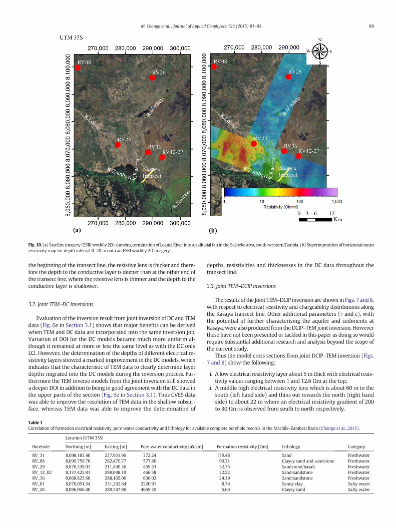
Fig. 10. (a) Satellite imagery (ESRIworldly 2D) showing termination of Loanja River into an alluvial fan in the Sesheke area, south-western Zambia. (b) Superimposition of horizontalmeanresistivity map for depth interval 0–20 m onto an ESRI worldly 2D Imagery.

89M. Chongo et al. / Journal of Applied Geophysics 123 (2015) 81–92

the beginning of the transect line, the resistive lens is thicker and there-fore the depth to the conductive layer is deeper than at the other end ofthe transect line, where the resistive lens is thinner and the depth to theconductive layer is shallower.

3.2. Joint TEM–DC inversions

Evaluation of the inversion result from joint inversion of DC and TEMdata (Fig. 6e in Section 3.1) shows that major benefits can be derivedwhen TEM and DC data are incorporated into the same inversion job.Variation of DOI for the DC models became much more uniform al-though it remained at more or less the same level as with the DC onlyLCI. However, the determination of the depths of different electrical re-sistivity layers showed amarked improvement in the DCmodels, whichindicates that the characteristic of TEM data to clearly determine layerdepths migrated into the DC models during the inversion process. Fur-thermore the TEM inverse models from the joint inversion still showeda deeper DOI in addition to being in good agreementwith the DC data inthe upper parts of the section (Fig. 6e in Section 3.1). Thus CVES datawas able to improve the resolution of TEM data in the shallow subsur-face, whereas TEM data was able to improve the determination of

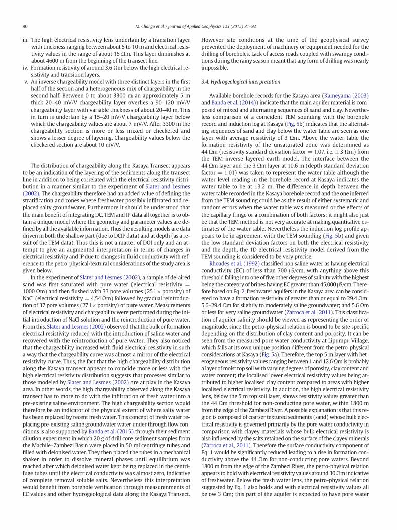
Table 1Correlation of formation electrical resistivity, pore water conductivity and lithology for availab

Borehole

Location [UTM 35S]

Pore water conductivity [μS/cm]Northing [m] Easting [m]

RV_31 8,098,183.40 237,931.96 372.24RV_08 8,099,759.76 262,479.77 577.80RV_29 8,076,339.01 211,449.36 459.53RV_12_02 8,137,425.81 299,048.19 466.58RV_36 8,068,825.60 288,165.00 636.02RV_01 8,070,051.34 231,262.64 2220.91RV_26 8,096,066.40 289,747.90 4659.35

depths, resistivities and thicknesses in the DC data throughout thetransect line.

3.3. Joint TEM–DCIP inversions

The results of the Joint TEM–DCIP inversion are shown in Figs. 7 and 8,with respect to electrical resistivity and chargeability distributions alongthe Kasaya transect line. Other additional parameters (τ and c), withthe potential of further characterising the aquifer and sediments atKasaya,were also produced from theDCIP–TEM joint inversion. Howeverthese have not been presented or tackled in this paper as doing so wouldrequire substantial additional research and analysis beyond the scope ofthe current study.

Thus the model cross sections from joint DCIP–TEM inversion (Figs.7 and 8) show the following:

i. A low electrical resistivity layer about 5m thickwith electrical resis-tivity values ranging between 1 and 12.6 Ωm at the top;

ii. A middle high electrical resistivity lens which is about 60 m in thesouth (left hand side) and thins out towards the north (right handside) to about 22 m where an electrical resistivity gradient of 200to 30 Ωm is observed from south to north respectively.

le complete borehole records in the Machile–Zambezi Basin (Chongo et al., 2015).

Formation resistivity [Ωm] Lithology Category

179.48 Sand Freshwater99.31 Clayey sand and sandstone Freshwater32.75 Sandstone/basalt Freshwater32.52 Sand/sandstone Freshwater24.19 Sand/sandstone Freshwater8.74 Sandy clay Salty water5.66 Clayey sand Salty water

90 M. Chongo et al. / Journal of Applied Geophysics 123 (2015) 81–92

iii. The high electrical resistivity lens underlain by a transition layerwith thickness ranging between about 5 to 10m and electrical resis-tivity values in the range of about 15 Ωm. This layer diminishes atabout 4600 m from the beginning of the transect line.

iv. Formation resistivity of around 3.6 Ωm below the high electrical re-sistivity and transition layers.

v. An inverse chargeability model with three distinct layers in the firsthalf of the section and a heterogeneous mix of chargeability in thesecond half. Between 0 to about 3300 m an approximately 5 mthick 20–40 mV/V chargeability layer overlies a 90–120 mV/Vchargeability layer with variable thickness of about 20–40 m. Thisin turn is underlain by a 15–20 mV/V chargeability layer belowwhich the chargeability values are about 7 mV/V. After 3300 m thechargeability section is more or less mixed or checkered andshows a lesser degree of layering. Chargeability values below thecheckered section are about 10 mV/V.

The distribution of chargeability along the Kasaya Transect appearsto be an indication of the layering of the sediments along the transectline in addition to being correlated with the electrical resistivity distri-bution in a manner similar to the experiment of Slater and Lesmes(2002). The chargeability therefore had an added value of defining thestratification and zones where freshwater possibly infiltrated and re-placed salty groundwater. Furthermore it should be understood thatthemain benefit of integrating DC, TEM and IP data all together is to ob-tain a unique model where the geometry and parameter values are de-fined by all the available information. Thus the resultingmodels are datadriven in both the shallow part (due to DCIP data) and at depth (as a re-sult of the TEM data). Thus this is not a matter of DOI only and an at-tempt to give an augmented interpretation in terms of changes inelectrical resistivity and IP due to changes in fluid conductivity with ref-erence to the petro-physical/textural considerations of the study area isgiven below.

In the experiment of Slater and Lesmes (2002), a sample of de-airedsand was first saturated with pure water (electrical resistivity =1000 Ωm) and then flushed with 33 pore volumes (25 l × porosity) ofNaCl (electrical resistivity = 4.54 Ωm) followed by gradual reintroduc-tion of 37 pore volumes (27 l × porosity) of pure water. Measurementsof electrical resistivity and chargeability were performed during the ini-tial introduction of NaCl solution and the reintroduction of pure water.From this, Slater and Lesmes (2002) observed that the bulk or formationelectrical resistivity reduced with the introduction of saline water andrecovered with the reintroduction of pure water. They also noticedthat the chargeability increased with fluid electrical resistivity in sucha way that the chargeability curve was almost a mirror of the electricalresistivity curve. Thus, the fact that the high chargeability distributionalong the Kasaya transect appears to coincide more or less with thehigh electrical resistivity distribution suggests that processes similar tothose modeled by Slater and Lesmes (2002) are at play in the Kasayaarea. In other words, the high chargeability observed along the Kasayatransect has to more to do with the infiltration of fresh water into apre-existing saline environment. The high chargeability section wouldtherefore be an indicator of the physical extent of where salty waterhas been replaced by recent fresh water. This concept of fresh water re-placing pre-existing saline groundwater water under through flow con-ditions is also supported by Banda et al. (2015) through their sedimentdilution experiment in which 20 g of drill core sediment samples fromthe Machile–Zambezi Basin were placed in 50 ml centrifuge tubes andfilled with deionised water. They then placed the tubes in a mechanicalshaker in order to dissolve mineral phases until equilibrium wasreached after which deionised water kept being replaced in the centri-fuge tubes until the electrical conductivity was almost zero, indicativeof complete removal soluble salts. Nevertheless this interpretationwould benefit from borehole verification through measurenments ofEC values and other hydrogeological data along the Kasaya Transect.

However site conditions at the time of the geophysical surveyprevented the deployment of machinery or equipment needed for thedrilling of boreholes. Lack of access roads coupled with swampy condi-tions during the rainy seasonmeant that any form of drillingwas nearlyimpossible.

3.4. Hydrogeological interpretation

Available borehole records for the Kasaya area (Kameyama (2003)and Banda et al. (2014)) indicate that the main aquifer material is com-posed of mixed and alternating sequences of sand and clay. Neverthe-less comparison of a coincident TEM sounding with the boreholerecord and induction log at Kasaya (Fig. 5b) indicates that the alternat-ing sequences of sand and clay below the water table are seen as onelayer with average resistivity of 3 Ωm. Above the water table theformation resistivity of the unsaturated zone was determined as44 Ωm (resistivity standard deviation factor = 1.07, i.e. ±3 Ωm) fromthe TEM inverse layered earth model. The interface between the44 Ωm layer and the 3 Ωm layer at 10.6 m (depth standard deviationfactor = 1.01) was taken to represent the water table although thewater level reading in the borehole record at Kasaya indicates thewater table to be at 13.2 m. The difference in depth between thewater table recorded in the Kasaya borehole record and the one inferredfrom the TEM sounding could be as the result of either systematic andrandom errors when the water table was measured or the effects ofthe capillary fringe or a combination of both factors; it might also justbe that the TEMmethod is not very accurate at making quantitative es-timates of the water table. Nevertheless the induction log profile ap-pears to be in agreement with the TEM sounding (Fig. 5b) and giventhe low standard deviation factors on both the electrical resistivityand the depth, the 1D electrical resistivity model derived from theTEM sounding is considered to be very precise.

Rhoades et al. (1992) classified non saline water as having electricalconductivity (EC) of less than 700 μS/cm, with anything above thisthreshold falling into one offive other degrees of salinitywith the highestbeing the category of brines having EC greater than 45,000 μS/cm. There-fore based on Eq. 2, freshwater aquifers in the Kasaya area can be consid-ered to have a formation resistivity of greater than or equal to 29.4 Ωm;5.6–29.4 Ωm for slightly to moderately saline groundwater; and 5.6 Ωmor less for very saline groundwater (Zarroca et al., 2011). This classifica-tion of aquifer salinity should be viewed as representing the order ofmagnitude, since the petro-physical relation is bound to be site specificdepending on the distribution of clay content and porosity. It can beseen from the measured pore water conductivity at Lipumpu Village,which falls at its own unique position different from the petro-physicalconsiderations at Kasaya (Fig. 5a). Therefore, the top 5 m layer with het-erogeneous resistivity values ranging between 1 and 12.6Ωmis probablya layer ofmoist top soilwith varying degrees of porosity, clay content andwater content; the localised lower electrical resistivity values being at-tributed to higher localised clay content compared to areas with higherlocalised electrical resistivity. In addition, the high electrical resistivitylens, below the 5 m top soil layer, shows resistivity values greater thanthe 44 Ωm threshold for non-conducting pore water, within 1800 mfrom the edge of the Zambezi River. A possible explanation is that this re-gion is composed of coarser textured sediments (sand) whose bulk elec-trical resistivity is governed primarily by the pore water conductivity incomparison with clayey materials whose bulk electrical resistivity isalso influenced by the salts retained on the surface of the clayeyminerals(Zarroca et al., 2011). Therefore the surface conductivity component ofEq. 1 would be significantly reduced leading to a rise in formation con-ductivity above the 44 Ωm for non-conducting pore waters. Beyond1800 m from the edge of the Zambezi River, the petro-physical relationappears to holdwith electrical resistivity values around 30Ωm indicativeof freshwater. Below the fresh water lens, the petro-physical relationsuggested by Eq. 1 also holds and with electrical resistivity values allbelow 3 Ωm; this part of the aquifer is expected to have pore water

91M. Chongo et al. / Journal of Applied Geophysics 123 (2015) 81–92

conductivity above 20,000 μS/cm. This distribution of electrical resistivityvalues along the Kasaya transect, into three distinct zones, indicates infil-tration of fresh surfacewater into a pre-existing saline aquifer. The inter-action of surfacewater and groundwater as suggested by the geophysicsis conceptualised in Fig. 9, and is probably driven by evapotranspirationand recharge from the Zambezi River.

In addition, the separation of the chargeability section (Fig. 7b)mid-way into a well layered part (0–3300 m) and a checkered part (3300–6600m) appears to correlate well with the extents of the plain and for-est areas. The layered chargeability section is in the plain whereas thecheckered chargeability section is in the forest. The reason for the highchargeability values and their distribution is unknown.

3.5. Regional scale perspectives

The landscape of the Machile–Zambezi Basin comprises a southerncentral low lying area (elevation between 900 and 950 m amsl)surrounded by moderate relief hilly areas from southeast to southwestin a clockwise direction. The drainage network is such that all streamsflow from the hilly areas into the low lying area and either terminateinto alluvial fans or eventually end up into the Zambezi River. It is there-fore likely that the groundwater regime in the upper reaches of thestream network is dominated by local flow systems with influentstreams (Sophocleous, 2002). From the transition between the hillyareas and the low lying area up to the Zambezi River the topography ex-hibits very low gradient. Consequently the groundwater flow is proba-bly dominated by intermediate and regional flow systems. Theseinteract with a seasonal flood cycle whereby the river system is influentduring flooding and effluent during the dry season (Main et al., 2008;Sophocleous, 2002). Thus surface water/groundwater interaction inthe Machile–Zambezi Basin can be said to be driven by recharge in thehigh elevation areas and a mix of seasonally alternating exfiltrationand infiltration in the moderate to low relief areas.

An evaluation of a satellite image encompassing the lower reaches ofthe Loanja River and the Kasaya area (Fig. 10a) shows themain channelof the Loanja River emerging from the high relief belt and broadeninginto an alluvial fan in the low relief region. Overlying the satelliteimage with a mean horizontal electrical resistivity map for depthinterval 0–20 m from the airborne TEM (Fig. 10b) shows that thealluvial fan is coincident with the higher electrical resistivity values. Asimilar observation can also be made about the Simalaha Floodplain(Chongo et al., 2015). The lack of borehole records along the KasayaTransect makes it extremely difficult to constrain the geophysical resultto geomorphological and hydro-chemical features. However Chongoet al. (2015) do give an interpretation of the regional electrical resistiv-ity distribution based on textural and pore fluid considerations that ingeneral associate high electrical resistivity values with coarser sedi-ments and low groundwater salinity; and low electrical resistivityvalues with intercalations of finer and coarser sediments and highgroundwater salinity as illustrated in Table 1 below.

4. Conclusion

A combination of TEM and DCIP measurements processed underjoint inversion provided insight into the nature of surface water/groundwater interaction on the northern bank of the Zambezi River atKasaya in southern Zambia. To our knowledge, this is the first timethat joint inversion of TEM and DCIP data has been conducted. Thejoint inversion showed a fresh water lens about 6.6 km in length fromthe edge of the Zambezi River. This was found to be about 60 m thickat the interface with the river and slowly thinned out further awayfrom the river until it reached a thickness of about 22 m at the end ofthe transect line. The fresh water lens is postulated to have had beenproduced by a combination of river interaction with the aquifer and in-fluenced by evapotranspiration. On a sub-regional scale, the hilly andhigher elevation areas of the Machile Zambezi Basin act as recharge

areas with influent streams, whereas the low lying areas interact witha seasonal flood cycle whereby the river system is influent duringflooding and effluent during the dry season.

Finally, the combination of DCIP and TEM data in a joint inversionproduced better inverse models with well resolved model parametersbased on DOI considerations. The TEM method was better at resolvingelectrical resistivities and thicknesses for the deeper layers whereasthe DC LCI produced inverse models with well resolved electrical resis-tivities and layer thicknesses in the shallow sub-surface but could notresolve these parameters at well enough at depth. However the DCmethod provided more data density. Joint inversion of DCIP and TEMdata thus produced a resultwith thebenefits of both high spatial densityand good determination of electrical resistivities and layer thicknessesboth in the shallow subsurface and the deeper subsurface. Including IPdata in the inversion had the added value of indicating the stratificationand zones where fresh surface water has probably infiltrated into thesub surface and replaced salty groundwater.

Acknowledgements

We are grateful to the Governments of the Republic of Zambia andthe Kingdom of Denmark for sponsoring this research under the capac-ity building initiative for the Zambianwater sector though the Universi-ty of Zambia. Special thanks also go to Dr. Chisengu Mdala, Lecturer inGeophysics at the University of Zambia and proprietor of AzuriteWater Resources (Ltd.) for allowing his field technician James Zulu toaccompany us if the field to collect the CVES and TEM data and to IngridMugamya at the UNZA IWRMCentre for logistical support. Furthermorewe are grateful to Erik Lange from DTU for facilitating the meeting withKurt Sørensen of SkyTEM that enabled us to borrow their WalkTEM in-strument for our fieldwork. We would also like to thank Kebby Kapika(District Water Officer — Sesheke, Western Province, Zambia),Mweemba Sinkombo (District Water Officer — Nalolo, WesternProvince, Zambia) and the community at Kasaya for moral and physicalsupport during the field measurements. Finally we would like to thankthe Hydro-geophysics group at Aarhus University for assistance duringprocessing and inversion of the TEM and CVES data sets.

Appendix A. Supplementary data

Supplementary data associated with this article can be found in theonline version, at doi: http://dx.doi.org/10.1016/j.jappgeo.2015.10.002.These data include the Google map of the most important areas de-scribed in this article.

References

ABEM(a), 2012. Terrameter LS User's Guide. ABEM Geophysics, Stockholm, p. 42.ABEM(b), 2014. WalkTEM User's Guide. ABEM Geophysics, Stockholm, p. 42.Aizebeokhai, A.P., 2010. 2D and 3D geoelectrical resistivity imaging: theory and field de-

sign. Sci. Res. Essays 5, 3592–3605.Albouy, Y., Andrieux, P., Rakotondrasoa, G., Ritz, M., Descloitres, M., Join, J.L.,

Rasolomanana, E., 2001. Mapping coastal aquifers by joint inversion of DC and TEMsoundings — three case histories. Ground Water 39, 87–97.

Aristodemou, E., Thomas-Betts, A., 2000. DC resistivity and induced polarisation investiga-tions at a waste disposal site and its environments. J. Appl. Geophys. 44, 275–302.

Auken, E., Christiansen, A.V., Jacobsen, B.H., Foged, N., Sorensen, K.I., 2005. Piecewise 1Dlaterally constrained inversion of resistivity data. Geophys. Prospect. 53, 497–506.

Auken, E., Christiansen, A.V., Kirkegaard, C., Fiandaca, G., Schamper, C., Behroozmand, A.A.,Binley, A., Nielsen, E., Efferso, F., Christensen, N.B.i., Sorensen, K., Foged, N., Vignoli, G.,2014. An Overview of a Highly Versatile Forward and Stable Inverse Algorithm forAirborne, Ground-Based and Borehole Electromagnetic and Electric Data. Explor.Geophys.

Banda, K.E., Jakobsenc, R., Gottwein, P.B., Murrayd, A.S., Nyambe, I., Larsen, F., 2014. TheLake Palaeo-Makgadikgadi in Western Zambia: Its Formation and Role in ProducingRecent Saline Groundwater, Unpublished Results. Geological Survey of Denmarkand Greenland, p. 47.

Banda, K.E., Jakobsen, R., Gottwein, P.B.-., Nyambe, I., Laier, T., Larsen, F., 2015. Identifica-tion and Evaluation of Hydro-Geochemical Processes in the Groundwater Environ-ment of Machile Basin, Western Zambia Unpublished Results. Technical Universityof Denmark, 2500kgs-Lynby, Denmark, Lynby, Denmark, p. 50.

92 M. Chongo et al. / Journal of Applied Geophysics 123 (2015) 81–92

Bauer, P., Supper, R., Zimmermann, S., Kinzelbach, W., 2006. Geoelectrical imaging ofgroundwater salinisation in the Okavango Delta, Botswana. J. Appl. Geophys. 60,126–141.

Behroozmand, A.A., Auken, E., Fiandaca, G., Christiansen, A.V., 2012. Improvement in MRSparameter estimation by joint and laterally constrained inversion of MRS and TEMdata. Geophysics 77.

Bertin, J., Loeb, J., 1969. Transients and field behaviour in induced polarization. Geophys.Prospect. 17, 488–510.

Binley, A., Kemna, A., 2006. DC Resistivity and Induced Polarization Methods. In: Rubin, Y.,Hubbard, S.S. (Eds.), Hydrogeophysics. Springer.

Brodie, R., Sundaram, B., Tottenham, R., Hostetler, S., Ransley, T., 2007. In: Forestry,D.o.A.i.a. (Ed.), An Overview of Tools for Assessing Groundwater–Surface Water Con-nectivity. Bureau of Rural Sciences, Canberra.

Chongo, M., Christiansen, A.V., Tembo, A., Banda, K.E., Nyambe, I.A., Larsen, F., Bauer-Gottwein, P., 2015. Airborne and ground based transient electromagnetic mappingof groundwater salinity in the Machile–Zambezi basin, south-western Zambia. NearSurf. Geophys. 13, 383–395.

Christiansen, A.V., Auken, E., 2012. A global measure for depth of investigation.Geophysics 77.

Christiansen, A.V., Esben, A., Sørensen, K., 2006. The Transient Electromagnetic Method.In: Kirsch, R. (Ed.), Groundwater Geophysics, A Tool for Hydrogeology. Springer,Flintbek, Germany.

Christiansen, A.V., Auken, E., Foged, N., Sorensen, K.I., 2007. Mutually and laterallyconstrained inversion of CVES and TEM data: a case study. Near Surf. Geophys. 5,115–123.

Dahlin, T., 2001. The development of DC resistivity imaging techniques. Comput. Geosci.27, 1019–1029.

Dahlin, T., Zhou, B., 2006. Multiple-gradient array measurements for multichannel 2D re-sistivity imaging. Near Surf. Geophys. 4, 113–123.

Dahlin, T., Leroux, V., Nissen, J., 2002. Measuring techniques in induced polarisation imag-ing. J. Appl. Geophys. 50, 279–298.

Danielsen, J.E., Auken, E., Jørgensen, F., Søndergaard, V., Sørensen, K.I., 2003. The applica-tion of the transient electromagnetic method in hydrogeophysical surveys. J. Appl.Geophys. 53, 181–198.

Danielsen, J.E., Dahlin, T., Owen, R., Mangeya, P., Auken, E., 2007. Geophysical andhydrogeologic investigation of groundwater in the Karoo stratigraphic sequence atSawmills in northern Matebeleland, Zimbabwe: a case history. Hydrogeol. J. 15,945–960.

ESRI, 2014. World Imagery.Ezersky, M., Legchenko, A., Al-Zoubi, A., Levi, E., Akkawi, E., Chalikakis, K., 2011. TEM study

of the geoelectrical structure and groundwater salinity of the Nahal Hever sinkholesite, Dead Sea shore, Israel. J. Appl. Geophys. 75, 99–112.

Fiandaca, G., Auken, E., Christiansen, A.V., Gazoty, A., 2012. Time-domain-induced polari-zation: full-decay forward modeling and 1D laterally constrained inversion of Cole–Cole parameters. Geophysics 77, E213–E225.

Fiandaca, G., Ramm, J., Binley, A., Gazoty, A., Christiansen, A.V., Auken, E., 2013. Resolvingspectral information from time domain induced polarization data through 2-D inver-sion. Geophys. J. Int. 192, 631–646.

Gazoty, A., Fiandaca, G., Pedersen, J., Auken, E., Christiansen, A.V., 2012a. Mapping of land-fills using time-domain spectral induced polarization data: the eskelund case study.Near Surf. Geophys. 10, 575–586.

Gazoty, A., Fiandaca, G., Pedersen, J., Auken, E., Christiansen, A.V., Pedersen, J.K., 2012b.Application of time domain induced polarization to the mapping of lithotypes in alandfill site. Hydrol. Earth Syst. Sci. 16, 1793–1804.

Gazoty, A., Fiandaca, G., Pedersen, J., Auken, E., Christiansen, A.V., 2013. Data repeatabilityand acquisition techniques for time-domain spectral induced polarization. Near Surf.Geophys. 11, 391–406.

Geonics, 2006. PROTEM 47D Operating Manual for 20/30 Gate Model. Geonics Limited,Ontario, Canada.

GEOTECH, 2011. Survey and Logistcs Report on a Helicopter Borne Versatile Time DomainElectromagnetic Survey on the Zambezi River Basin Kazungula Zambia for Ministry ofEnergy and Water Development (Republic of Zambia). Geotech Airborne Limited,West Indies, p. 20.

Guerin, R., Descloitres, M., Coudrain, A., Talbi, A., Gallaire, R., 2001. Geophysical surveys foridentifying saline groundwater in the semi-arid region of the central altiplano,Bolivia. Hydrol. Process. 15, 3287–3301.

Harthill, N., 1976. Time-domain electromagnetic sounding. IEEE Trans. Geosci. Electron.14, 256–260.

Johnson, I.M., 1984. Spectral induced polarization parameters as determined throughtime-domain measurements. Geophysics 49.

Kameyama, N., 2003. Completion Report: JICA Borehole Drilling Project-Sesheke. Ministryof Energy and Water Development, Lusaka.

Kirsch, R., 2009. Groundwater Geophysics : A Tool for Hydrogeology.Loke, M.H., 1999. Electrical Imaging Surveys for Environmental and Engineering Studies,

A Practical Guide to 2-D and 3-D Surveys (Malaysia).Loke, M.H., Chambers, J.E., Rucker, D.F., Kuras, O., Wilkinson, P.B., 2013. Recent develop-

ments in the direct-current geoelectrical imaging method. J. Appl. Geophys. 95,135–156.

Main, M.P.L., Moore, A.E., Williams, H.B., Cotterill, F.P.D., 2008. The Zambezi River. LargeRivers, Geomorphology and Management, pp. 311–332.

Marescot, L., Monnet, R., Chapellier, D., 2008. Resistivity and induced polarization surveysfor slope instability studies in the Swiss Alps. Eng. Geol. 98, 18–28.

Milosevic, N., Thomsen, N.I., Juhler, R.K., Albrechtsen, H.J., Bjerg, P.L., 2012. Identification ofdischarge zones and quantification of contaminant mass discharges into a localstream from a landfill in a heterogeneous geologic setting. J. Hydrol. 446, 13–23.

Mualem, Y., Friedman, S.P., 1991. Theoretical prediction of electrical-conductivity in satu-rated and unsaturated soil. Water Resour. Res. 27, 2771–2777.

Nabighian, M.N., 1991. Electromagnetic Methods in Applied Geophysics Vol. 2, Electro-magnetic Methods in Applied Geophysics Vol. 2.

Nassir, S.S.A., Loke, M.H., Lee, C.Y., Nawawi, M.N.M., 2000. Salt-water intrusion mappingby geoelectrical imaging surveys. Geophys. Prospect. 48, 647–661.

Oldenburg, D.W., Li, Y.G., 1999. Estimating depth of investigation in dc resistivity and IPsurveys. Geophysics 64, 403–416.

Pelton, W.H., Ward, S.H., Hallof, P.G., Sill, W.R., Nelson, P.H., 1978. Mineral discriminationand removal of inductive coupling with multifrequency IP. Geophysics 43, 588–609.

Rhoades, J.D., Manteghi, N.A., Shouse, P.J., Alves, W.J., 1989. Soil electrical-conductivityand soil-salinity — new formulations and calibrations. Soil Sci. Soc. Am. J. 53,433–439.

Rhoades, J.D., Kandiah, A., Mashali, A.M., 1992. The use of Saline Waters for Crop Production— FAO Irrigation and Drainage Paper 48. Food and Agriculture Organization of the Unit-ed Nations, Rome.

Roy, A., Apparao, A., 1971. Depth of investigation in direct current methods. Geophysics36, 943–959.

Rubin, Y., Hubbard, S.S., 2006. Hydrogeophysics. Springer.Shalem, Y., Weinstein, Y., Levi, E., Herut, B., Goldman, M., Yechieli, Y., 2014. The Extent of

Aquifer Salinization next to an Estuarine River, an Example from the EasternMediter-ranean. Hydrogeology Journal.

Shanafield, M., Cook, P.G., 2014. Transmission losses, infiltration and groundwater re-charge through ephemeral and intermittent streambeds: a review of appliedmethods. J. Hydrol. 511, 518–529.

Slater, L.D., Lesmes, D., 2002. IP interpretation in environmental investigations. Geophys-ics 67, 77–88.

Sonkamble, S., Kumar, V.S., Amarender, B., Dhunde, P.M., Sethurama, S., Kumar, K.R., 2014.Delineation of fresh aquifers in tannery belt for sustainable development — a casestudy from southern India. J. Geol. Soc. India 83, 279–289.

Sophocleous, M., 2002. Interactions between groundwater and surface water: the state ofthe science. Hydrogeol. J. 10, 52–67.

Spies, B.R., 1989. Depth of investigation in electromagnetic sounding methods. Geophys-ics 54, 872–888.

Titov, K., Komarov, V., Tarasov, V., Levitski, A., 2002. Theoretical and experimental study oftime domain-induced polarization in water-saturated sands. J. Appl. Geophys. 50,417–433.

Vaudelet, P., Schmutz, M., Pessel, M., Franceschi, M., Guerin, R., Atteia, O., Blondel, A.,Ngomseu, C., Galaup, S., Rejiba, F., Begassat, P., 2011. Mapping of contaminant plumeswith geoelectrical methods. A case study in urban context. J. Appl. Geophys. 75,738–751.

Vilhelmsen, T.N., Behroozmand, A.A., Christensen, S., Nielsen, T.H., 2014. Joint inversion ofaquifer test, MRS, and TEM data. Water Resour. Res. 50, 3956–3975.

Weller, A., Slater, L., Nordsiek, S., 2013. On the relationship between induced polarizationand surface conductivity: implications for petrophysical interpretation of electricalmeasurements. Geophysics 78, D315–D325.

Westbrook, S.J., Rayner, J.L., Davis, G.B., Clement, T.P., Bjerg, P.L., Fisher, S.T., 2005. Interac-tion between shallow groundwater, saline surface water and contaminant dischargeat a seasonally and tidally forced estuarine boundary. J. Hydrol. 302, 255–269.

Winter, T.C., 1999. Relation of streams, lakes, and wetlands to groundwater flow systems.Hydrogeol. J. 7, 28–45.

Xue, G.-q., Bai, C.-y., Yan, S., Greenhalgh, S., Li, M.-f., Zhou, N.-n., 2012. Deep sounding TEMinvestigation method based on a modified fixed central-loop system. J. Appl.Geophys. 76, 23–32.

Zarroca, M., Bach, J., Linares, R., Pellicer, X.M., 2011. Electrical methods (VES and ERT) foridentifying, mapping and monitoring different saline domains in a coastal plain re-gion (Alt Emporda, Northern Spain). J. Hydrol. 409, 407–422.

Zarroca, M., Linares, R., Rodellas, V., Garcia-Orellana, J., Roqué, C., Bach, J., Masqué, P.,2014. Delineating coastal groundwater discharge processes in a wetland area bymeans of electrical resistivity imaging, 224Ra and 222Rn. Hydrol. Process. 28,2382–2395.

Zarroca, M., Linares, R., Velásquez-López, P.C., Roqué, C., Rodríguez, R., 2015. Applica-tion of electrical resistivity imaging (ERI) to a tailings dam project for artisanaland small-scale gold mining in Zaruma-Portovelo, Ecuador. J. Appl. Geophys.113, 103–113.

Zhou, S., Yuan, X., Peng, S., Yue, J., Wang, X., Liu, H., Williams, D.D., 2014. Groundwater–Surface Water Interactions in the Hyporheic Zone Under Climate Change Scenarios.Environmental Science and Pollution Research.