Journal of Applied Geophysics 85 (2012) 59–67

Contents lists available at SciVerse ScienceDirect

Journal of Applied Geophysics

j ourna l homepage: www.e lsev ie r .com/ locate / jappgeo

Regularizing dipole polarizabilities in time-domain electromagnetic inversion

Laurens Beran a,b,⁎, Stephen Billings b, Douglas Oldenburg a

a Department of Earth and Ocean Sciences, University of British Columbia, 6339 Stores Road, Vancouver, B.C., Canada V6T 1Z4b Sky Research Inc., Suite 112A, 2386 East Mall Vancouver, B.C., Canada V6T 1Z3

⁎ Corresponding author at: Tel.: +1 541 525 5149;E-mail address: lberan@eos.ubc.ca (L. Beran).

0926-9851/$ – see front matter © 2012 Elsevier B.V. Alldoi:10.1016/j.jappgeo.2012.06.011

a b s t r a c t

a r t i c l e i n f o

Article history:Received 6 February 2012Accepted 26 June 2012Available online 5 July 2012

Keywords:Unexploded ordnanceDiscriminationElectromagneticsRegularized inversion

Recent advances in time-domain electromagnetic (TEM) sensors have dramatically improved discriminationof buried unexploded ordnance (UXO). In contrast to commercial standard mono-static sensors, themulti-static, multi-component geometries of next generation TEM sensors provide diverse excitations of adetected target. Inversion of observed data using the parametric TEM dipole model typically produceswell-constrained estimates that can subsequently be inputted into a discrimination algorithm. In particular,the principal dipole polarizabilities provide information about target size and shape. Shape is represented bytwo transverse polarizabilities orthogonal to a target's axis of symmetry.Equality of transverse polarizabilities is diagnostic of an axisymmetric body of revolution and so has beenproposed as a useful feature to discriminate between axisymmetric UXO and non-axisymmetric metallic clut-ter. Here we show that estimated transverse polarizabilities can sometimes be poorly constrained in an inver-sion of multi-static TEM data. This motivates our development of a regularized inversion algorithm thatpenalizes the deviation between transverse polarizabilities. We then develop an extension of the supportvector machine (SVM) classifier that uses all models obtained via regularized inversion to make discrimina-tion decisions. This approach achieves the best performance of all candidate discrimination algorithms ap-plied to a number of real data sets.

© 2012 Elsevier B.V. All rights reserved.

1. Introduction

The 2003 Defense Science Board report on unexploded ordnance(UXO) projected that a reduction in false alarm rates from 100:1 to10:1would save $36 billion on remediation projects within the UnitedStates (Delaney and Etter, 2003). This cost reduction was expected tobe achieved by improvements in sensor and data processing technolo-gies. These goals havebeenmet, and sometimes exceeded, in recent dem-onstration projects conducted by the Environmental Security TechnologyCertification Program (ESTCP) (Billings et al., 2010, Prouty et al., 2011,Shubitidze et al., 2011, Steinhurst et al., 2010). Advances in electromag-netic (EM) sensors have been crucial to these successes: the data provid-ed by multi-static, multi-component EM platforms are much improvedinputs into the inversion and discrimination algorithms applied to thisproblem. Fig. 1 compares the geometry and time channels of the com-mercial standard Geonics EM-61 with two multi-static EM instrumentsdesigned for UXO discrimination. The Time-domain Electro-MagneticMulti-sensor Towed Array Detection System (TEMTADS, shown inFig. 1b) is composed of an array of 25 horizontal transmitter loops ar-ranged in a 5×5 grid, with horizontal receivers measuring the verticalfield arranged concentrically to these transmitters (Steinhurst et al.,2010). The transmitters are fired sequentially and the secondary fieldresponse is recorded in all receivers simultaneously. This configuration

fax: +1 541 488 4606.

rights reserved.

provides a diverse data set which is better able to constrain target pa-rameters. The MetalMapper sensor (Fig. 1c) has also greatly improvedthe reliability of estimated parameters by transmitting orthogonal pri-mary fields and measuring all components of the secondary field inmultiple tri-axial receivers (Prouty et al., 2011). Both MetalMapperand TEMTADS systems are deployed in a static (or cued) mode:previously-detected targets are interrogated with a stationary sensor.A mono-static sensor such as the EM61 has to be moved to several po-sitions to illuminate a detected target and success of this process is crit-ically dependent on accurate geolocation (Tantum et al., 2008, TarokhandMiller, 2007). The single static acquisition requiredwhen deployingTEMTADS or MetalMapper sensors thereby removes the need for accu-rate geolocation.

In this paper we study parameter estimation with multi-static sen-sor data. We show that while these data generally support inversionand discrimination, in some cases parameter estimates can be poorlyconstrained. This motivates regularization of the inverse problem andhere we seek models corresponding to targets with axial symmetry.This property is diagnostic of many UXO and so provides a useful fea-ture for classifying targets of interest. We investigate methods formodel selection and develop a technique that uses all models from reg-ularized inversion tomake discrimination decisions.We also extendourregularized inversion technique to multi-object scenarios to deal withoverlapping target anomalies. Finally, we apply our techniques to datasets from ESTCP live-site demonstrations and compare discriminationperformance.

Fig. 1. (a) EM-61, (b) TEMTADS, and (c) MetalMapper sensors for unexploded ordnance detection and discrimination. Top row shows sensor geometry, with solid and dashed linesindicating receiver and transmitter coils, respectively. Bottom row shows logarithmically-spaced time channels.

60 L. Beran et al. / Journal of Applied Geophysics 85 (2012) 59–67

2. Parameter estimation with the dipole model

The time (or frequency) dependent dipole model is essential tomost electromagnetic data processing for UXO discrimination (Bellet al., 2001b, Pasion and Oldenburg, 2001, Zhang et al., 2003). WhileShubitidze and collaborators have also achieved excellent discrimina-tion results with more “physically complete” models (e.g. Shubitidzeet al., 2011), our focus in this article is on improving discriminationwith the dipole model in challenging scenarios.

The dipole model provides a simple parametric representation ofthe response of a confined conductor. The rate of change of the sec-ondary magnetic field is computed as

∂Bs

∂t r; tð Þ ¼ p tð Þr3

3 p̂ tð Þ⋅r̂ð Þr̂−p̂ tð Þð Þ ð1Þ

with r ¼ rr̂ the separation between target and observation location,and p tð Þ ¼ p tð Þp̂ tð Þ a time-varying dipole moment

p tð Þ ¼ 1μo

P tð Þ⋅Bo: ð2Þ

The induced dipole is the projection of the primary field Bo ontothe target's polarizability tensor P(t) (Bell et al., 2001b). Here the ele-ments of the polarizability tensor (Pij(t)) represent the convolution ofthe target's B-field impulse response ˜P tð Þð Þwith the transmitter wave-form i(t) (Wait, 1982)

Pij tð Þ ¼ ∂∂t ∫

∞

−∞P̃ij t′−t

� �i t′� �

dt′: ð3Þ

The polarizability tensor is assumed to be symmetric and positivedefinite and so it can be decomposed as

P tð Þ ¼ ATL tð ÞA ð4Þ

with A an orthogonal matrix which rotates the coordinate system fromgeographic coordinates to a local, body centered coordinate system. Thediagonal eigenvalue matrix L(t) contains the principal polarizabilitiesLi(t) (i=1,2,3),which are assumed to be independent of target orienta-tion and location.

Features derived from the dipole model have been successfully usedto discriminate between targets of interest (TOI) andnon-hazardousme-tallic clutter. In particular the amplitude and decay of the principal polar-izabilities provide a simple parameter set for discrimination (Beran et al.,

2011). For a sensorwithN channels, these target features can be comput-ed as

amplitude ¼XNj¼1

Ltotal tj� �

decay tk; tj� �

¼ Ltotal tkð ÞLtotal tj

� � ð5Þ

with the total polarizability Ltotal(tj) defined as the sumof the polarizabil-ities at each time channel

Ltotal tj� �

¼X3i¼1

Li tj� �

: ð6Þ

The decay parameter is a ratio of total polarizabilities at selectedchannels. For tk> tj we have decay(tk, tj)b1, so that a larger decay pa-rameter is diagnostic of a slow decaying total polarizability.

The amplitude and decay parameters are physically meaningfulbecause, to first order, a confined conductor can be modeled as a simpleLR loopwhich is inductively coupled to transmitters and receivers on thesurface. The current response of this loop is a decaying exponentialwhich is fully described by an amplitude and time constant (West andMacnae, 1991). In practice, many larger UXO (e.g. 105 mm projectiles,81 mmmortars) produce large amplitude, slow decaying polarizabilitiesrelative to metallic debris. However, at more challenging sites withsmaller items (e.g. 37 mm projectiles, fuzes), amplitude and decay pa-rameters alone may not be sufficient to reliably discriminate UXO fromclutter of similar size.

The TEM dipole model generalizes the simple circuit model to ac-count for target shape. A ferrous, prolate (rod-like) targetwith rotation-al symmetry about its principal axis will produce equal transverse(secondary and tertiary) polarizabilities (Bell et al., 2001b). For ferrousitems, internal demagnetization is strongly affected by the shape of theobject. The result is that the strength of the induced dipoles along thesemi-minor axes is reduced, so that transverse polarizabilities are smallerin magnitude than axial polarizabilities.

Most ordnance are composed primarily of steel and can be treatedas bodies of revolution (Bell et al., 2001a, Shubitidze et al., 2002,Zhang et al., 2003) and so equality of transverse polarizabilities hasbeen proposed as a useful feature for discriminating between TOIand irregularly-shaped clutter. However, in practice it has been diffi-cult to reliably estimate target shape frommono-static TEM data. Thisis because single loop, vertical-component transmitters and receiversoften cannot adequately interrogate the transverse response of buried

0.8

Transverse (x)

y (

m)

0

−0.8

−0.8

0 0.8

Transverse (y)

−0.8 0x (m)

0.8

Axial (z)

−0.8 0 0.8

Data

−0.8 0 0.8

(mV/A)−10 0 10

Fig. 3. Components of the dipole response over a spherical target (same as in 2) for the5×5 TEMTADS array. Each subplot shows the received field at all receivers excited bythe corresponding transmitter in the array. Data units for the TEMTADS result fromnormalization of the received EMF by the transmitter current.

61L. Beran et al. / Journal of Applied Geophysics 85 (2012) 59–67

targets. Fig. 2 illustrates this effect for a spherical target illuminatedby a mono-static Geonics EM-61 sensor (geometry and time channelsare shown in Fig. 1).

In the case of a sphere all polarizabilities are equal, and so here wedefine the primary, axial polarizability as aligned along the z axis. Thecorresponding induced field is maximal when the sensor is directlyover the target. However to excite the transverse (x and y) responsesof the target the sensor must be positioned with a horizontal stand-offfrom the target. Assuming an approximately dipolar field radiated fromtransmitter and target, the secondary field (Eq. (1)) decays as 1/r6 withincreasing sensor–target separation r. For this reason, the axial polariz-ability response dominates the measured data in Fig. 2. Data which aresensitive to transverse polarizabilities therefore tend to have low signalto noise, particularly for vertically-oriented targets. This geometric effectis exacerbated by the reduced amplitude of transverse polarizabilities forferrous ordnance. These factors confounded early attempts to estimatetarget shape from mono-static sensors (e.g. Bell et al., 2001b).

Multi-static TEM sensors designed for UXO detection have helpedaddress these limitations. Fig. 3 shows the components of the dipoleresponse for the TEMTADS sensor over the same target as in Fig. 2.The data received for transmitters immediately adjacent to the centertransmitter are primarily sensitive to a combination of the transverseexcitations. Inversion of these data therefore produces better con-strained estimates of transverse polarizabilities than can be obtainedwithmono-static sensor data. This is illustrated in Fig. 4, which comparespolarizabilities estimated fromEM-61,MetalMapper, and TEMTADS dataacquired over the same 37 mm projectile. Here we quantify the discrep-ancy between transverse polarizabilities with the asymmetry parameter

ς ¼ 1N

XNi

L2 tið Þ−L3 tið Þð Þ=L2 tið Þ: ð7Þ

The estimated polarizabilities at each channel are sorted so thatL1≥L2≥L3, implying ςb1. An ideal axisymmetric target with equaltransverse polarizabilities will have ς=0. For the example in Fig. 4the cued sensors produce a significantly smaller asymmetry parame-ter than the EM-61 (paired t-tests, 95% confidence level).

We note, however, that at late times the transverse polarizabilitiesestimated from TEMTADS and MetalMapper data begin to divergedue to decreased signal to noise. This effect is exacerbated when thecued sensors are not properly positioned directly over the target. InFig. 5 we show two inversion results for MetalMapper data acquiredover a 37 mm projectile. In the first data collection the target isnear the edge of the sensor and the resulting transverse polarizabil-ities are poorly constrained. Repositioning the sensor over the targetin Fig. 5(b) significantly reduces the estimated asymmetry.

−1 0 1

Axial (z)

−1 0 1

Transverse (y)

x (m)−1 0 1

Data

(mV)0 40 80

−1 0 1−1

0

1Transverse (x)

y (m

)

Fig. 2. Components of the dipole response over a target positioned at r=[0, 0,−0.3]mfor the EM-61. Predicted data are a linear combination of axial and transverse re-sponses, here for a spherical target with polarizabilities Li=1, i=1,2,3. Excitation oftransverse responses requires a horizontal standoff, resulting in a lower SNR than foraxial excitation.

While multi-static sensors can greatly improve the reliability ofestimated polarizabilities, we conclude from the preceding examplesthat challenging scenarios with low SNR can still result in poorly con-strained secondary polarizabilities that will confound an algorithmthat incorporates these parameters to make discrimination decisions.

Here we investigate techniques for explicitly constraining transversepolarizability estimateswhen invertingmulti-static sensor data. An obvi-ous and viable approach to this problem is to simply reparameterize thedipole model so that secondary and tertiary polarizabilities are equal.Practical use of this axisymmetric dipole model is motivated by the ana-lytic response of a spheroid and by successful fits to high-fidelity teststand data acquired over real axisymmetric targets (Pasion, 2007). Ofcourse, this model will not provide a good fit to data acquired over anon-axisymmetric target with three unique polarizabilities.

A data processing approach which has been proposed to handlethis ambiguity is to fit each target using both axisymmetric and non-axisymmetric (i.e. unequal transverse) dipole parameterizations andthen to compare the fits to the observed data (Pasion, 2007). The non-axisymmetric parameterization has more degrees of freedom that canbe used to fit observed data and so generally provides a lower misfitthan the axisymmetric dipole parameterization. The problem is thento determine what constitutes a significant difference in data misfit forthe two competing parameterizations. Model selection criteria can beused to select the most parsimonious model parameterization whichcan explain the data (Hastie et al., 2001).

In this work we instead apply regularization techniques to con-strain the polarizabilities estimated from TEMTADS and MetalMapperdata sets. Constraints on model parameters are typically applied inthe form of parameter bounds, here we will impose an additionalconstraint in the form of a penalty on unequal transverse polarizabil-ities. This approach provides us with a continuum of possible modelsbetween constrained and unconstrained models (or, equivalently, be-tween axisymmetric and non-axisymmetric dipole parameterizations).We investigatemethods for selecting amodel, or set ofmodels, from reg-ularized inversion. Finally, we show applications to data sets from ESTCPdemonstrations at San Luis Obispo (SLO), CA, and Camp Butner, NC.

3. Regularized inversion

When solving parametric inverse problems, it is often sufficient tominimize a data norm quantifying the misfit between observed andpredicted data

ϕd ¼ Wd dobs−dpred� �2 ð8Þ

with dpred=F(m) generally a nonlinear functional of the model m,and Wd a weighting matrix accounting for estimated errors on thedata. Assuming Gaussian errors on the observed data, minimizationof Eq. (8) yields a maximum likelihood estimate of the model parame-ters (Menke, 1989). Additional prior information can be incorporated

1e−05

1e−03

1e−01

1

0.04

0.22

1.27

24.3

5

Pol

ariz

abili

ties

(arb

.)

EM−61: ς =0.62

Time (ms)

L 1

L 2

L 3

1e−05

1e−03

1e−01

1

0.04

0.11

7.91

24.3

5

MetalMapper: ς =0.24

Time (ms)

1e−05

1e−03

1e−01

1

0.04

24.3

5

TEMTADS: ς =0.35

Time (ms)

Fig. 4. Estimated dipole polarizabilities for a 37 mm projectile buried at 10 cm. The primary polarizability at channel 1 is normalized to 1 for each sensor. Abscissa limits in all plotscorrespond to the time range of the TEMTADS sensor. The asymmetry parameter ς is defined in Eq. (7).

62 L. Beran et al. / Journal of Applied Geophysics 85 (2012) 59–67

in the inversion via parameter bounds (e.g. positivity) or by constructingamodelwhichhas specifiedproperties. In the latter case, the optimizationproblem can be solved byminimizing the norm (Oldenburg and Li, 2005)

minϕ ¼ ϕd þ βϕm: ð9Þ

where the regularization parameterβ controls the trade-off between dataand model norms. The model norm ϕm is a regularizer that ensures thatthe recovered model has, for example, a minimum deviation from someprior reference model. Aliamiri et al. (2007) employed a regularizationof this form for estimation of dipole model parameters, with the regular-ization parameter fixed a priori. An even stronger regularization of the in-verse problem is developed in Pasion et al. (2007): theyfix polarizabilitiesat library values for each ordnance class. They then fit the observed datafor target location and orientation and use the data misfit as a metricfor ranking targets. This requires multiple inversions of each anomaly(one for each ordnance class) and cannot be easily generalized to multi-object scenarios.

Here we instead apply a regularizer which addresses the problemof poorly constrained transverse polarizabilities. In the case of the di-pole model, an appropriate model norm which penalizes differencesin secondary and tertiary polarizabilities is

ϕm ¼ L2−L3ð Þ2¼ jjWmmjj2 ð10Þ

10−1

100

101

1e−5

1

Time (ms)

Pol

ariz

abili

ties

(arb

.)

(a)

−0.5 0 0.5−0.5

0

0.5

x (m)

y (m

)

10−1

100

101

1e−5

1

Time (ms)

(b)

L1

L2

L3

−0.5 0 0.5−0.5

0

0.5

x (m)

y (m

)

Fig. 5. Top row: estimated polarizabilities for two soundings with the MetalMapperover the same 37 mm projectile (a different 37 mm than in Fig. 4). Bottom row: esti-mated target locations (blue circles) for these soundings, relative to the sensor. Blacksquares indicate receivers and red dashed lines are transmitters.

with Wm a model weighting matrix acting as a differencing operatoron the appropriate elements of themodel vectorm. For a linear forwardmodeling (dpred=Gm) with fixed β, the model estimate is obtained bysolving the system (Oldenburg and Li, 2005)

GTWTdWdGþ βWT

mWm

� �m ¼ GTWT

dWddobs

: ð11Þ

In practice, the inverse problem can be solved by minimizing Eq. (9)over a range of β values, beginning with a large value of β and progres-sively decreasing (or “cooling”) this parameter (Oldenburg and Li,2005). When regularizing overdetermined problems the model has lim-ited degrees of freedom with which to fit the data and so the β coolingprocedure will stall at a model corresponding to the unconstrained(β=0) solution. This is in contrast to the underdetermined inverse prob-lem,where continued decrease of the regularization parameter eventual-ly introduces spurious model structure.

Following on the works of Shubitidze et al. (2007) and Song et al.(2011), we use a sequential inversion approach that decouples esti-mation of target location and dipole polarizabilities. The predicteddata can be expressed as

dpred ¼ G rð ÞmP: ð12Þ

Here the model mP is composed of the six unique elements of thesymmetric polarizability tensor P at a single time channel

mP ¼ Pxx; Pxy; Pxz; Pyy; Pyz; Pzz

h iT: ð13Þ

The forward modeling matrix is

G rð Þ ¼

BxsB

xp

BxsB

yp þ By

s Bxp

BxsB

zp þ Bz

sBxp

BysB

yp

Bys B

zp þ Bz

sByp

BzsB

zp

2666666664

3777777775

T

ð14Þ

with Bp the primary field at the target and Bs the secondary field atthe receiver, with all fields implicitly dependent upon target (r)and sensor location. Superscripts denote the x,y,z components ofthe respective fields. We then solve the regularized inverse problemas follows:

1 Solve an inverse problem for target location r. The model is relatedto the predicted data via the nonlinear functional

dpred ¼ F r½ � ¼ G rð ÞG† rð Þdobs: ð15Þ

with G† denoting the pseudo-inverse. We estimate r by minimiza-tion of Eq. (8) using an iterative Gauss–Newton algorithm.

5 10 15 2010

−5

100

(a)

Channel

Pol

ariz

abili

ties

(arb

.)

L1

L2

L3

5 10 15 2010

−5

100

(b)

Channel

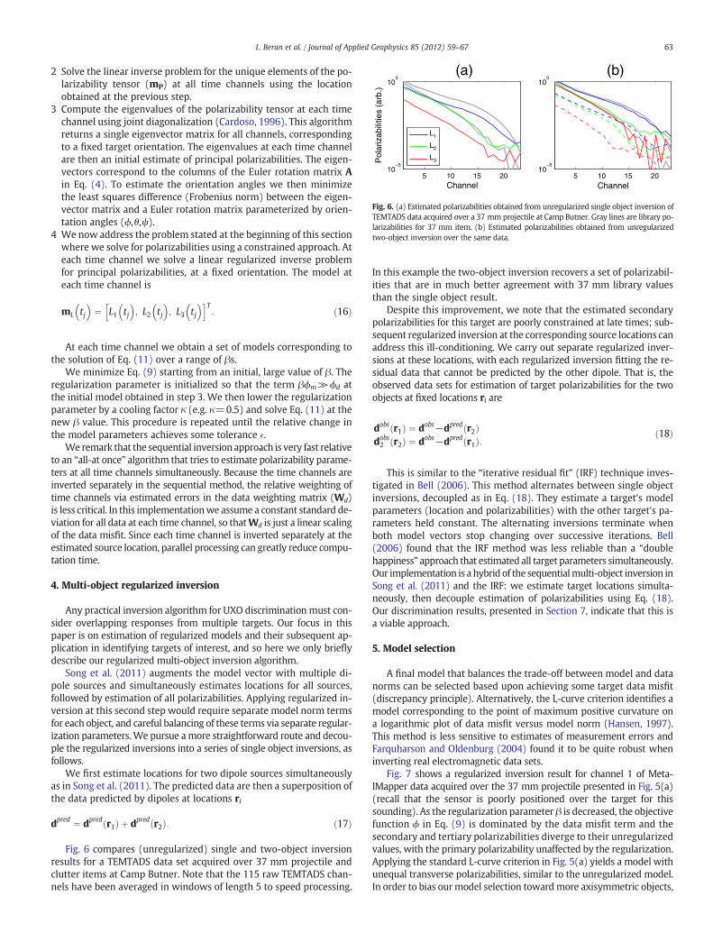
Fig. 6. (a) Estimated polarizabilities obtained from unregularized single object inversion ofTEMTADS data acquired over a 37 mm projectile at Camp Butner. Gray lines are library po-larizabilities for 37 mm item. (b) Estimated polarizabilities obtained from unregularizedtwo-object inversion over the same data.

63L. Beran et al. / Journal of Applied Geophysics 85 (2012) 59–67

2 Solve the linear inverse problem for the unique elements of the po-larizability tensor (mP) at all time channels using the locationobtained at the previous step.

3 Compute the eigenvalues of the polarizability tensor at each timechannel using joint diagonalization (Cardoso, 1996). This algorithmreturns a single eigenvector matrix for all channels, correspondingto a fixed target orientation. The eigenvalues at each time channelare then an initial estimate of principal polarizabilities. The eigen-vectors correspond to the columns of the Euler rotation matrix Ain Eq. (4). To estimate the orientation angles we then minimizethe least squares difference (Frobenius norm) between the eigen-vector matrix and a Euler rotation matrix parameterized by orien-tation angles (ϕ,θ,ψ).

4 We now address the problem stated at the beginning of this sectionwhere we solve for polarizabilities using a constrained approach. Ateach time channel we solve a linear regularized inverse problemfor principal polarizabilities, at a fixed orientation. The model ateach time channel is

mL tj� �

¼ L1 tj� �

; L2 tj� �

; L3 tj� �h iT

: ð16Þ

At each time channel we obtain a set of models corresponding tothe solution of Eq. (11) over a range of βs.

We minimize Eq. (9) starting from an initial, large value of β. Theregularization parameter is initialized so that the term βϕm≫ϕd atthe initial model obtained in step 3. We then lower the regularizationparameter by a cooling factor κ (e.g. κ=0.5) and solve Eq. (11) at thenew β value. This procedure is repeated until the relative change inthe model parameters achieves some tolerance �.

We remark that the sequential inversion approach is very fast relativeto an “all-at once” algorithm that tries to estimate polarizability parame-ters at all time channels simultaneously. Because the time channels areinverted separately in the sequential method, the relative weighting oftime channels via estimated errors in the data weighting matrix (Wd)is less critical. In this implementationwe assume a constant standard de-viation for all data at each time channel, so thatWd is just a linear scalingof the data misfit. Since each time channel is inverted separately at theestimated source location, parallel processing can greatly reduce compu-tation time.

4. Multi-object regularized inversion

Any practical inversion algorithm for UXO discrimination must con-sider overlapping responses from multiple targets. Our focus in thispaper is on estimation of regularized models and their subsequent ap-plication in identifying targets of interest, and so here we only brieflydescribe our regularized multi-object inversion algorithm.

Song et al. (2011) augments the model vector with multiple di-pole sources and simultaneously estimates locations for all sources,followed by estimation of all polarizabilities. Applying regularized in-version at this second step would require separate model norm termsfor each object, and careful balancing of these terms via separate regular-ization parameters. We pursue amore straightforward route and decou-ple the regularized inversions into a series of single object inversions, asfollows.

We first estimate locations for two dipole sources simultaneouslyas in Song et al. (2011). The predicted data are then a superposition ofthe data predicted by dipoles at locations ri

dpred ¼ dpred r1ð Þ þ dpred r2ð Þ: ð17Þ

Fig. 6 compares (unregularized) single and two-object inversionresults for a TEMTADS data set acquired over 37 mm projectile andclutter items at Camp Butner. Note that the 115 raw TEMTADS chan-nels have been averaged in windows of length 5 to speed processing.

In this example the two-object inversion recovers a set of polarizabil-ities that are in much better agreement with 37 mm library valuesthan the single object result.

Despite this improvement, we note that the estimated secondarypolarizabilities for this target are poorly constrained at late times; sub-sequent regularized inversion at the corresponding source locations canaddress this ill-conditioning. We carry out separate regularized inver-sions at these locations, with each regularized inversion fitting the re-sidual data that cannot be predicted by the other dipole. That is, theobserved data sets for estimation of target polarizabilities for the twoobjects at fixed locations ri are

dobs r1ð Þ ¼ dobs−dpred r2ð Þdobs2 r2ð Þ ¼ dobs−dpred r1ð Þ: ð18Þ

This is similar to the “iterative residual fit” (IRF) technique inves-tigated in Bell (2006). This method alternates between single objectinversions, decoupled as in Eq. (18). They estimate a target's modelparameters (location and polarizabilities) with the other target's pa-rameters held constant. The alternating inversions terminate whenboth model vectors stop changing over successive iterations. Bell(2006) found that the IRF method was less reliable than a “doublehappiness” approach that estimated all target parameters simultaneously.Our implementation is a hybrid of the sequentialmulti-object inversion inSong et al. (2011) and the IRF: we estimate target locations simulta-neously, then decouple estimation of polarizabilities using Eq. (18).Our discrimination results, presented in Section 7, indicate that this isa viable approach.

5. Model selection

A final model that balances the trade-off between model and datanorms can be selected based upon achieving some target data misfit(discrepancy principle). Alternatively, the L-curve criterion identifies amodel corresponding to the point of maximum positive curvature ona logarithmic plot of data misfit versus model norm (Hansen, 1997).This method is less sensitive to estimates of measurement errors andFarquharson and Oldenburg (2004) found it to be quite robust wheninverting real electromagnetic data sets.

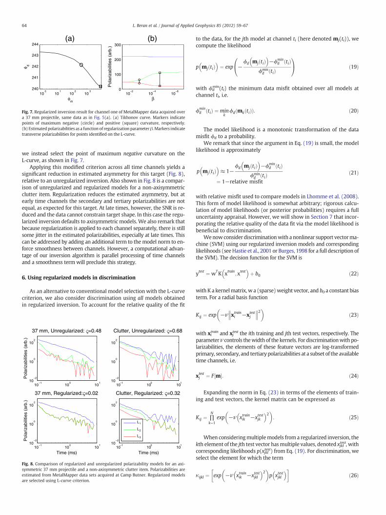
Fig. 7 shows a regularized inversion result for channel 1 of Meta-lMapper data acquired over the 37 mm projectile presented in Fig. 5(a)(recall that the sensor is poorly positioned over the target for thissounding). As the regularization parameter β is decreased, the objectivefunction ϕ in Eq. (9) is dominated by the data misfit term and thesecondary and tertiary polarizabilities diverge to their unregularizedvalues, with the primary polarizability unaffected by the regularization.Applying the standard L-curve criterion in Fig. 5(a) yields a model withunequal transverse polarizabilities, similar to the unregularized model.In order to bias ourmodel selection towardmore axisymmetric objects,

100

101

102

103

240

241

242

243

244

φm

φ d

(a)

10−6

10−4

10−20

100

200

300

Pol

ariz

abili

ties

(arb

.)

β

(b)

Fig. 7. Regularized inversion result for channel one of MetalMapper data acquired overa 37 mm projectile, same data as in Fig. 5(a). (a) Tikhonov curve. Markers indicatepoints of maximum negative (circle) and positive (square) curvature, respectively.(b) Estimated polarizabilities as a function of regularization parameterβ. Markers indicatetransverse polarizabilities for points identified on the L-curve.

64 L. Beran et al. / Journal of Applied Geophysics 85 (2012) 59–67

we instead select the point of maximum negative curvature on theL-curve, as shown in Fig. 7.

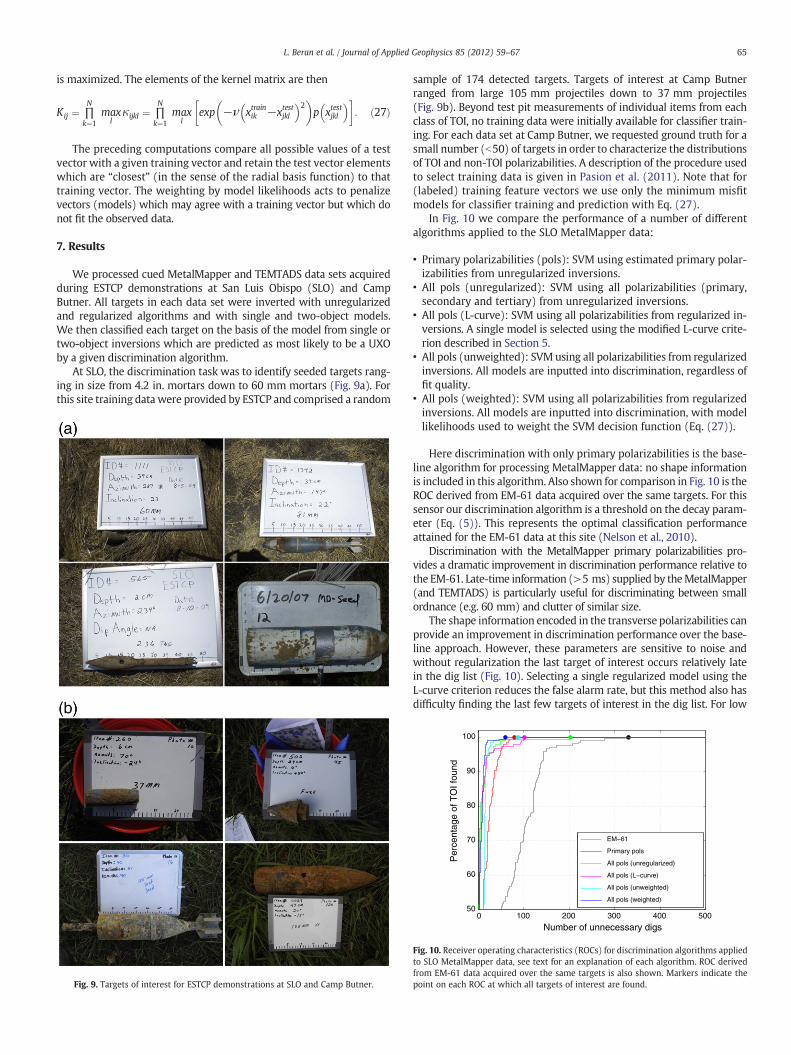
Applying this modified criterion across all time channels yields asignificant reduction in estimated asymmetry for this target (Fig. 8),relative to an unregularized inversion. Also shown in Fig. 8 is a compar-ison of unregularized and regularized models for a non-axisymmetricclutter item. Regularization reduces the estimated asymmetry, but atearly time channels the secondary and tertiary polarizabilities are notequal, as expected for this target. At late times, however, the SNR is re-duced and the data cannot constrain target shape. In this case the regu-larized inversion defaults to axisymmetric models. We also remark thatbecause regularization is applied to each channel separately, there is stillsome jitter in the estimated polarizabilities, especially at late times. Thiscan be addressed by adding an additional term to themodel norm to en-force smoothness between channels. However, a computational advan-tage of our inversion algorithm is parallel processing of time channelsand a smoothness term will preclude this strategy.

6. Using regularized models in discrimination

As an alternative to conventional model selection with the L-curvecriterion, we also consider discrimination using all models obtainedin regularized inversion. To account for the relative quality of the fit

10−1

100

101

10−2

100

102

37 mm, Unregularized: ς=0.48

Pol

ariz

abili

ties

(arb

.)

10−1

100

101

10−2

100

102

37 mm, Regularized:ς=0.02

Time (ms)

Pol

ariz

abili

ties

(arb

.)

10−1

100

101

10−2

100

102

Clutter, Unregularized: ς=0.68

10−1

100

101

10−2

100

102

Clutter, Regularized: ς=0.32

Time (ms)

L1

L2

L3

Fig. 8. Comparison of regularized and unregularized polarizability models for an axi-symmetric 37 mm projectile and a non-axisymmetric clutter item. Polarizabilities areestimated from MetalMapper data sets acquired at Camp Butner. Regularized modelsare selected using L-curve criterion.

to the data, for the jth model at channel ti (here denoted mj(ti)), wecompute the likelihood

p mj tið Þ� �

¼ exp −ϕd mj tið Þ

� �−ϕmin

d tið Þϕmind tið Þ

0@

1A ð19Þ

with ϕdmin(ti) the minimum data misfit obtained over all models at

channel ti, i.e.

ϕmind tið Þ ¼ min

kϕd mk tið Þð Þ: ð20Þ

The model likelihood is a monotonic transformation of the datamisfit ϕd to a probability.

We remark that since the argument in Eq. (19) is small, the modellikelihood is approximately

p mj tið Þ� �

≈ 1−ϕd mj tið Þ

� �−ϕmin

d tið Þϕmind tið Þ

¼ 1−relative misfit

ð21Þ

with relative misfit used to compare models in Lhomme et al. (2008).This form of model likelihood is somewhat arbitrary; rigorous calcu-lation of model likelihoods (or posterior probabilities) requires a fulluncertainty appraisal. However, we will show in Section 7 that incor-porating the relative quality of the data fit via the model likelihood isbeneficial to discrimination.

Wenowconsider discriminationwith a nonlinear support vectorma-chine (SVM) using our regularized inversion models and correspondinglikelihoods (seeHastie et al., 2001 or Burges, 1998 for a full description ofthe SVM). The decision function for the SVM is

ytest ¼ wTK xtrain;xtest� �

þ b0 ð22Þ

with K a kernelmatrix, w a (sparse)weight vector, and b0 a constant biasterm. For a radial basis function

Kij ¼ exp −ν xtraini −xtest

j

��� ���2� �

ð23Þ

with xitrain and xjtest the ith training and jth test vectors, respectively. Theparameterν controls thewidth of the kernels. For discriminationwith po-larizabilities, the elements of these feature vectors are log-transformedprimary, secondary, and tertiary polarizabilities at a subset of the availabletime channels, i.e.

xtestj ¼ F m½ �: ð24Þ

Expanding the norm in Eq. (23) in terms of the elements of train-ing and test vectors, the kernel matrix can be expressed as

Kij ¼ ∏N

k¼1exp −ν xtrainik −xtestjk

� �2� �

: ð25Þ

When consideringmultiplemodels from a regularized inversion, thekth element of the jth test vector hasmultiple values, denoted xjkl

test, withcorresponding likelihoods p(xjkltest) from Eq. (19). For discrimination, weselect the element for which the term

κ ijkl ¼ exp −ν xtrainik −xtestjkl

� �2� �

p xtestjkl

� �� �ð26Þ

65L. Beran et al. / Journal of Applied Geophysics 85 (2012) 59–67

is maximized. The elements of the kernel matrix are then

Kij ¼ ∏N

k¼1max

lκ ijkl ¼ ∏

N

k¼1max

lexp −ν xtrainik −xtestjkl

� �2� �

p xtestjkl

� �� �: ð27Þ

The preceding computations compare all possible values of a testvector with a given training vector and retain the test vector elementswhich are “closest” (in the sense of the radial basis function) to thattraining vector. The weighting by model likelihoods acts to penalizevectors (models) which may agree with a training vector but which donot fit the observed data.

7. Results

We processed cued MetalMapper and TEMTADS data sets acquiredduring ESTCP demonstrations at San Luis Obispo (SLO) and CampButner. All targets in each data set were inverted with unregularizedand regularized algorithms and with single and two-object models.We then classified each target on the basis of the model from single ortwo-object inversions which are predicted as most likely to be a UXOby a given discrimination algorithm.

At SLO, the discrimination task was to identify seeded targets rang-ing in size from 4.2 in. mortars down to 60 mm mortars (Fig. 9a). Forthis site training data were provided by ESTCP and comprised a random

Fig. 9. Targets of interest for ESTCP demonstrations at SLO and Camp Butner.

sample of 174 detected targets. Targets of interest at Camp Butnerranged from large 105 mm projectiles down to 37 mm projectiles(Fig. 9b). Beyond test pit measurements of individual items from eachclass of TOI, no training data were initially available for classifier train-ing. For each data set at Camp Butner, we requested ground truth for asmall number (b50) of targets in order to characterize the distributionsof TOI and non-TOI polarizabilities. A description of the procedure usedto select training data is given in Pasion et al. (2011). Note that for(labeled) training feature vectors we use only the minimum misfitmodels for classifier training and prediction with Eq. (27).

In Fig. 10 we compare the performance of a number of differentalgorithms applied to the SLO MetalMapper data:

• Primary polarizabilities (pols): SVM using estimated primary polar-izabilities from unregularized inversions.

• All pols (unregularized): SVM using all polarizabilities (primary,secondary and tertiary) from unregularized inversions.

• All pols (L-curve): SVM using all polarizabilities from regularized in-versions. A single model is selected using the modified L-curve crite-rion described in Section 5.

• All pols (unweighted): SVM using all polarizabilities from regularizedinversions. All models are inputted into discrimination, regardless offit quality.

• All pols (weighted): SVM using all polarizabilities from regularizedinversions. All models are inputted into discrimination, with modellikelihoods used to weight the SVM decision function (Eq. (27)).

Here discrimination with only primary polarizabilities is the base-line algorithm for processing MetalMapper data: no shape informationis included in this algorithm. Also shown for comparison in Fig. 10 is theROC derived from EM-61 data acquired over the same targets. For thissensor our discrimination algorithm is a threshold on the decay param-eter (Eq. (5)). This represents the optimal classification performanceattained for the EM-61 data at this site (Nelson et al., 2010).

Discrimination with the MetalMapper primary polarizabilities pro-vides a dramatic improvement in discrimination performance relative tothe EM-61. Late-time information (>5 ms) supplied by theMetalMapper(and TEMTADS) is particularly useful for discriminating between smallordnance (e.g. 60 mm) and clutter of similar size.

The shape information encoded in the transverse polarizabilities canprovide an improvement in discrimination performance over the base-line approach. However, these parameters are sensitive to noise andwithout regularization the last target of interest occurs relatively latein the dig list (Fig. 10). Selecting a single regularized model using theL-curve criterion reduces the false alarm rate, but this method also hasdifficulty finding the last few targets of interest in the dig list. For low

0 100 200 300 400 50050

60

70

80

90

100

Number of unnecessary digs

Per

cent

age

of T

OI f

ound

EM−61

Primary pols

All pols (unregularized)

All pols (L−curve)

All pols (unweighted)

All pols (weighted)

Fig. 10. Receiver operating characteristics (ROCs) for discrimination algorithms appliedto SLO MetalMapper data, see text for an explanation of each algorithm. ROC derivedfrom EM-61 data acquired over the same targets is also shown. Markers indicate thepoint on each ROC at which all targets of interest are found.

66 L. Beran et al. / Journal of Applied Geophysics 85 (2012) 59–67

SNR targets the Tikhonov curve has a small curvature and it becomesdifficult to accurately identify the L-curve criterion. The weighted SVMachieves the best discrimination performance for algorithms appliedto the SLOMetalMapper data. The benefit of weighting by model likeli-hoods is illustrated in Fig. 10 by the reduction in false alarm rate relativeto using unweighted models.

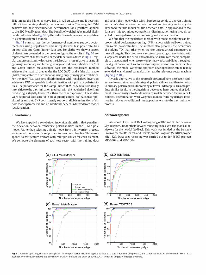
Fig. 11 summarizes the performance of nonlinear support vectormachines using regularized and unregularized test polarizabilitieson both SLO and Camp Butner data sets. For clarity we show a subsetof algorithms presented in the previous figure, the results in Fig. 10 arerepresentative of all test cases. For the data sets considered in Fig. 11, reg-ularization consistently decreases the false alarm rate relative to using all(primary, secondary and tertiary) unregularized polarizabilities. For SLOand Camp Butner MetalMapper data sets the regularized methodachieves the maximal area under the ROC (AUC) and a false alarm rate(FAR) comparable to discrimination using only primary polarizabilities.For the TEMTADS data sets, discrimination with regularized inversionachieves a FAR comparable to discrimination with primary polarizabil-ities. The performance for the Camp Butner TEMTADS data is relativelyinsensitive to the discriminationmethod, with the regularized algorithmproducing a slightly lower FAR than the other approach. These datawere acquired with careful in-field quality control so that sensor po-sitioning and data SNR consistently support reliable estimation of di-pole model parameters and no additional benefit is derived frommodelregularization.

8. Conclusions

We have applied a regularized inversion algorithm that penalizesthe deviation between transverse polarizabilities in the TEM dipolemodel. Rather than selecting a singlemodel from this inversion process,we input all models into a support vector machine classifier. This corre-sponds to test feature vectors with multiple values for each element.We compare the elements of each test vector with the training data

0 100 200 300 400 50050

60

70

80

90

100

Number of unnecessary digs

Per

cent

age

of T

OI f

ound

EM−61Primary polsAll pols (unregularized)All pols (weighted)

0 500 1000 1500 200050

60

70

80

90

100

Number of unnecessary digs

Per

cent

age

of T

OI f

ound

(a) SLO MetalMapper

(c) Butner MetalMapper (

Fig. 11. Receiver operating characteristics (ROCs) for support vector machines applied to cuacquired over the same targets are also shown. Markers indicate the point on each ROC at

and retain the model value which best corresponds to a given trainingvector. We also penalize the match of test and training vectors by thelikelihood that the model fits the observed data. In applications to realdata sets this technique outperforms discrimination using models se-lected from regularized inversion using an L-curve criterion.

We find that the regularized method with model weighting can im-prove initial performance on high SNR targets with well-constrainedtransverse polarizabilities. The method also prevents the occurrenceof outlying TOI that arise when we use unregularized parameters torank all targets. This produces a receiver operating characteristic witha large area under the curve and a final false alarm rate that is compara-ble to that obtainedwhenwe rely on primary polarizabilities throughoutthe dig list. While we have focused on support vector machines for clas-sification, the model weighting approach developed here can be readilyextended to any kernel based classifier, e.g. the relevance vectormachine(Tipping, 2001).

A viable alternative to the approach presented here is to begin rank-ing well-constrainedmodels using all polarizabilities, and then to switchto primary polarizabilities for ranking of lower SNR targets. This can pro-duce similar results to the algorithms developed here, but requires judg-ment from an analyst to decide when to switch between feature sets. Incontrast, discrimination with weighted models from regularized inver-sion introduces no additional tuning parameters into the discriminationprocess.

Acknowledgments

Wewould like to thankDr. Lin-Ping Songof UBC andDr. Len Pasion ofSky Research, Inc. for their forwardmodeling codes.We also thank all re-viewers for the helpful feedback. This work was funded by the StrategicEnvironmental Research and Development Program (SERDP) projectMR-1629. Data preprocessing was carried out under ESTCP projectsMR-0504 and MR-1004.

0 100 200 300 400 50050

60

70

80

90

100

Number of unnecessary digs

Per

cent

age

of T

OI f

ound

0 500 1000 1500 200050

60

70

80

90

100

Number of unnecessary digs

Per

cent

age

of T

OI f

ound

(b) SLO TEMTADS

d) Butner TEMTADS

ed data sets at San Luis Obispo (SLO) and Camp Butner. ROCs derived from EM-61 datawhich all targets of interest are found.

67L. Beran et al. / Journal of Applied Geophysics 85 (2012) 59–67

References

Aliamiri, A., Stalnaker, J., Miller, E.L., 2007. Statistical classification of buried unexplodedordnance using nonparametric prior models. IEEE Transactions on Geoscience andRemote Sensing 45, 2794–2806.

Bell, T., 2006. Adaptive and Iterative Processing Techniques for Overlapping Signatures:Technical Summary Report, ESTCP Project MM-200415. Technical Report. ESTCP.

Bell, T., Barrow, B., Miller, J., Keiswetter, D., 2001a. Time and frequency domain electro-magnetic induction signatures of unexploded ordinance. Subsurface Sensing Tech-nologies and Applications 2, 153–175.

Bell, T., Barrow, B., Miller, J.T., 2001b. Subsurface discrimination using electromagnetic in-duction sensors. IEEE Transactions on Geoscience and Remote Sensing 39, 1286–1293.

Beran, L.S., Billings, S.D., Oldenburg, D., 2011. Incorporating uncertainty in unexplodedordnance discrimination. IEEE Transactions on Geoscience and Remote Sensing 49,3071–3080.

Billings, S.D., Pasion, L.R., Beran, L., Lhomme, N., Song, L., Oldenburg, D.W., Kingdon, K.,Sinex, D., Jacobson, J., 2010. Unexploded ordnance discrimination using magneticand electromagnetic sensors: case study from a former military site. Geophysics 75,B103–B114.

Burges, C.J.C., 1998. A tutorial on support vector machines for pattern recognition. DataMining and Knowledge Discovery 2, 955–974.

Cardoso, J.F., 1996. Jacobi angles for simultaneous diagonalization. SIAM Journal onMatrix Analysis and Applications 17, 161–163.

Delaney, W.P., Etter, D., 2003. Report of the Defense Science Board on unexploded ord-nance. Technical Report. Office of the Undersecretary of Defense for Acquisition,Technology and Logistics.

Farquharson, C.G., Oldenburg, D.W., 2004. A comparison of automatic techniques forestimating the regularization parameter in non-linear inverse problems. GeophysicalJournal International 156, 411–425.

Hansen, P.C., 1997. Rank-deficient and discrete ill-posed problems: numerical aspectsof linear inversion. SIAM.

Hastie, T., Tibshirani, R., Friedman, J., 2001. The Elements of Statistical Learning: DataMining, Inference and Prediction. Spring-Verlag.

Lhomme, N., Oldenburg, D.W., Pasion, L.R., Sinex, D., Billings, S.D., 2008. Assessing thequality of electromagnetic data for the discrimination of UXO using figures ofmerit. Journal of Engineering and Environmental Geophysics 13, 165–176.

Menke, W., 1989. Geophysical Data Analysis: Discrete Inverse Theory. Academic Press.Nelson, H.H., Andrews, A., Kaye, K., 2010. ESTCP pilot program: classification approaches

in munitions response, San Luis Obispo, California. Technical Report. ESTCP.Oldenburg, D., Li, Y., 2005. Investigations in Geophysics No. 13: near-surface. Society

of Exploration Geophysics. Chapter Inversion for Applied Geophysics: A Tutorial,pp. 89–150.

Pasion, L.R., 2007. Inversion of time-domain electromagnetic data for the detection ofunexploded ordnance. Ph.D. thesis. University of British Columbia.

Pasion, L.R., Oldenburg, D.W., 2001. A discrimination algorithm for UXO using time domainelectromagnetic induction. Journal of Environmental and Engineering Geophysics 6,91–102.

Pasion, L.R., Billings, S.D., Oldenburg, D.W., Walker, S., 2007. Application of a library-based method to time domain electromagnetic data for the identification ofunexploded ordnance. Journal of Applied Geophysics 61, 279–291.

Pasion, L.R., Beran, L.S., Zelt, B.C., Kingdon, K.A., 2011. Feature extraction and classifica-tion of EMI data, Camp Butner, NC, ESTCP project MR-201004. Technical Report.ESTCP.

Prouty, M., George, D.C., Snyder, D.D., 2011. MetalMapper: a multi-sensor TEM systemfor UXO detection and classification, ESTCP project MR-200603. Technical Report.ESTCP.

Shubitidze, F., O'Neill, K., Haider, S.A., Sun, K., Paulsen, K.D., 2002. Application of themethod of auxiliary sources to the wide-band electromagnetic induction problem.IEEE Transactions on Geoscience and Remote Sensing 40, 928–942.

Shubitidze, F., O'Neill, K., Barrowes, B., Shamatava, I., Fernández, J., Sun, K., Paulsen, K.,2007. Application of the normalized surface magnetic charge model to UXO dis-crimination in cases with overlapping signals. Journal of Applied Geophysics 61,292–303.

Shubitidze, F., Barrowes, B., Shamatava, I., Fernandez, J.P., O'Neill, K., 2011. The orthonormalized volume magnetic source technique applied to live-site UXO data: in-version and classification studies. SEG Technical Program Expanded Abstracts 30,3766–3770.

Song, L.P., Pasion, L.R., Billings, S.D., Oldenburg, D., 2011. Nonlinear inversion for multipleobjects in transient electromagnetic induction sensing of unexploded ordnance:technique and applications. IEEE Transactions on Geoscience and Remote Sensing49, 4007–4020.

Steinhurst, D.A., Harbaugh, G.R., Kingdon, J.B., Furuya, T., Keiswetter, D.A., George, D.C.,2010. EMI array for cued UXO discrimination, ESTCP project MM-0601. TechnicalReport. ESTCP.

Tantum, S.L., Li, Y., Collins, L.M., 2008. Bayesian mitigation of sensor position errors toimprove unexploded ordnance detection. IEEE Geoscience and Remote SensingLetters 5, 103–107.

Tarokh, A.B., Miller, E.L., 2007. Subsurface sensing under sensor positional uncertainty.IEEE Transactions on Geoscience and Remote Sensing 45, 675–688.

Tipping, M.E., 2001. Sparse Bayesian learning and the relevance vector machine. Journalof Machine Learning Research 1, 211–244.

Wait, J.R., 1982. Geo-electromagnetism. Academic Press.West, G.F., Macnae, J.C., 1991. Electromagnetic methods in applied geophysics. SEG.

Chapter physics of the electromagnetic exploration method, pp. 5–45.Zhang, Y., Collins, L.M., Yu, H., Baum, C.E., Carin, L., 2003. Sensing of unexploded ord-

nance with magnetometer and induction data: theory and signal processing. IEEETransactions on Geoscience and Remote Sensing 41, 1005–1015.