global precipitation: a 17-year monthly analysis based on ...zli/meto620/readings for aosc424... ·...

2539Bulletin of the American Meteorological Society

1. Introduction

Despite the increasing requirements for high-qual-ity precipitation datasets from both the meteorologi-cal and hydrological communities, accurate quantita-tive documentation of global precipitation remains asone of the major challenges for scientists working ontechnique development and dataset construction, prin-cipally because of the large spatial and temporal vari-ability in precipitation and because of the lack of acomprehensive observing system (WCRP 1993). Themajor existing sources of large-scale precipitation datainclude gauge observations, estimates inferred from

satellite observations, and outputs from various nu-merical models, each of which has advantages as wellas shortcomings.

Generally speaking, rain gauges give relatively ac-curate point measurements of precipitation but sufferfrom sampling error in representing area means andare not available over most oceanic and unpopulatedland areas. Satellite observations of infrared (IR) andmicrowave (MW) radiance have been used success-fully to retrieve precipitation information over manyparts of the globe (Barrett and Martin 1981; Arkin andArdanuy 1989), but the estimates made from satelliteobservations contain nonnegligible random error andbias because of the indirect nature of the relationshipbetween the observation and the precipitation, the in-adequate sampling, and algorithm imperfections. Ingeneral, different satellite estimates based on a givensort of observation data (IR, MW scattering, or MWemission) exhibit similar skills, while those based on

Global Precipitation: A 17-YearMonthly Analysis Based on Gauge

Observations, Satellite Estimates,and Numerical Model Outputs

Pingping Xie and Phillip A. ArkinNational Centers for Environmental Prediction,

National Oceanic and Atmospheric Administration, Washington, D.C.

ABSTRACT

Gridded fields (analyses) of global monthly precipitation have been constructed on a 2.5° latitude–longitude grid forthe 17-yr period from 1979 to 1995 by merging several kinds of information sources with different characteristics, in-cluding gauge observations, estimates inferred from a variety of satellite observations, and the NCEP–NCAR reanaly-sis. This new dataset, which the authors have named the CPC Merged Analysis of Precipitation (CMAP), contains pre-cipitation distributions with full global coverage and improved quality compared to the individual data sources. Exami-nations showed no discontinuity during the 17-yr period, despite the different data sources used for the different subperiods.Comparisons of the CMAP with the merged analysis of Huffman et al. revealed remarkable agreements over the globalland areas and over tropical and subtropical oceanic areas, with differences observed over extratropical oceanic areas.The 17-yr CMAP dataset is used to investigate the annual and interannual variability in large-scale precipitation. Themean distribution and the annual cycle in the 17-yr dataset exhibit reasonable agreement with existing long-term meansexcept over the eastern tropical Pacific. The interannual variability associated with the El Niño–Southern Oscillationphenomenon resembles that found in previous studies, but with substantial additional details, particularly over the oceans.With complete global coverage, extended period and improved quality, the 17-yr dataset of the CMAP provides veryuseful information for climate analysis, numerical model validation, hydrological research, and many other applications.Further work is under way to improve the quality, extend the temporal coverage, and to refine the resolution of the mergedanalysis.

Corresponding author address: Dr. Pingping Xie, National Cen-ters for Environmental Prediction, #800A, NOAA/NWS, Wash-ington, DC 20233.E-mail: [email protected] final form 25 June 1997.©1997 American Meteorological Society

2540 Vol. 78, No. 11, November 1997

different sources of data vary more from one anotherin their performance in estimating precipitation overvarious areas and for various seasons. In general, how-ever, most such estimates yield relatively good (poor)results for tropical oceanic (cold season extratropicalland) precipitation (Xie and Arkin 1995; Janowiak etal. 1995). The precipitation distributions produced byvarious numerical models, meanwhile, exhibit rela-tively high quality in mid- and high latitudes but per-form more poorly over most tropical areas (Arpe1991). After a comprehensive examination of severalindividual datasets of large-scale precipitation, Xieand Arkin (1995) concluded that all of these individualdata sources present similar distribution patterns oflarge-scale precipitation but with differences insmaller-scale features and in amplitudes and that atleast three major deficiencies exist in the individualdata sources: 1) incomplete global coverage, 2) sig-nificant random error, and 3) nonnegligible bias.

Acknowledgment of the limitations inherent in theindividual sources of large-scale precipitation has led tosome recent attempts to combine them so as to take ad-vantage of the strengths of each to produce the best pos-sible analysis (gridded field) of global precipitation. Onesuch effort is reported by Adler et al. (1993, 1994),Huffman et al. (1995), and Huffman et al. (1997). As-suming that estimates based on MW observationsfrom the Special Sensor Microwave/Imager (SSM/I)on board the DMSP satellites give relatively accurateinstantaneous rain rate but with poor sampling in timeand that the GOES Precipitation Index (GPI; Arkinand Meisner 1987) estimates based on IR observationsfrom geostationary satellites provide frequent coveragebut with significant bias, Adler et al. (1993) and Adleret al. (1994) calculate the ratio between the MW andthe GPI estimates when both are available and use theratio to adjust the GPI estimates. Their multisatellite(MS) estimates, comprised of the adjusted GPI from40°S to 40°N and the MW estimates elsewhere, arethen multiplied by the ratio between the concurrentgauge observations and the MS calculated over a large-scale area to correct the bias. Finally, gauge observa-tions are combined with the bias-corrected MS estimatesusing optimal coefficients that are inversely propor-tional to the error variance of each source (Huffman etal. 1995). An 8.5-yr analysis of global monthly pre-cipitation based on this algorithm has been constructedand published for the period from July 1987 to De-cember 1995 (Huffman et al. 1997) and is used by theGlobal Precipitation Climatology Project (GPCP;Arkin and Xie 1994) as its official final product.

Another approach to this problem is that of Xie andArkin (1996), in which gauge observations, threekinds of satellite estimates (based on IR, MW scat-tering, and MW emission methods), and numericalmodel predictions are merged in two steps. First, toreduce the random error, the satellite estimates and themodel predictions are combined linearly through themaximum likelihood estimation method, in which theweighting coefficients are inversely proportional to theerror variance for the individual data source. Each ofthe included datasets has some characteristic thatmakes it likely that it adds information to the combi-nation. The IR estimates are based on more frequentsampling than the others, the microwave estimates arebased on observations of raindrops and ice particles,rather than cloud tops, and the model predictions in-corporate information on atmospheric mass and mo-tion. In principal, the linear combination of thesedatasets will have smaller random errors than any ofthem individually. Any bias in the individual datasets,however, remains in the combination. To remove thatbias, the output of the first step is then blended withthe gauge observations using the method of Reynolds(1988), in which the gauge data and the first-step-out-put are used to define the amplitude and the relativedistribution, or “shape,” of the precipitation field, re-spectively. Sensitivity tests showed that the quality ofthe merged analysis has been improved substantiallycompared to the individual data sources, with randomerror reduced significantly and bias removed almostcompletely (Xie and Arkin 1996). A comprehensiveintercomparison conducted recently by Adler et al.(1996) as a part of the NASA WetNet project (Dodge1994) found that the merged analyses of Xie and Arkin(1996) and Huffman et al. (1997) performed best inrepresenting large-scale precipitation among over 30participating products based on one or a combinationof various information sources.

The GPCP analysis of Huffman et al. (1997) relyupon estimates based on satellite observations that arenot generally available for the period before 1986, forthe GPI, and mid-1987, for the microwave-based es-timates. Many applications of the global precipitationdatasets in climate analysis, model validation, andhydrological research, however, call for longer peri-ods of record beginning from 1979 or earlier (Gates1992; Schubert et al. 1993; Kalney et al. 1996), andthe GPCP is investigating methods of producing suchdatasets. In this paper, we describe an experimentalextension of the merged analysis of Xie and Arkin(1996) to cover the period from 1979 to 1995, both to


investigate the problems involved in making such anextension, and to provide users with a product bettersuited to diagnostic analyses for this entire period thanany previously available. The lessons learned in the pro-duction of this dataset, and through its use in diagnosticstudies, will increase the chances of a successful exten-sion of the official GPCP product to cover this period.

To make possible the extension of our mergedanalysis, other satellite estimates of reasonable qual-ity must be found. Recently, Xie and Arkin (1997)developed a new technique, which they called the out-going longwave radiation (OLR)-based PrecipitationIndex (OPI), to estimate global monthly precipitationfrom the satellite-observed OLR data that are avail-able from June 1974 to the present, except for a 10-month missing period from March to December 1978.Estimates based on the new technique are able to pro-vide nearly complete global coverage of large-scaleprecipitation with high quality for most areas over theglobe and for all seasons. Together with the gauge-based analysis of Xie et al. (1996) over land and theoceanic estimates of Spencer (1993) based on obser-vations from the Microwave Sounding Unit (MSU),estimates based on the OPI technique provide a use-ful means to quantitatively describe the global distri-butions of large-scale precipitation continuously foran extended period from 1979 to the present.

In this paper, we describe a time series of globalmonthly precipitation analyses on a 2.5° latitude–lon-gitude grid for the 17-yr period from 1979 to 1995 andsome of its applications in the analysis of annual andinterannual variability in large-scale precipitation.This analysis was produced by merging gauge obser-vations, a number of satellite estimates, including theIR-based GPI, OLR-based OPI, MSU-based Spencer,MW-scattering-based NOAA/NESDIS (Grody 1991;Ferraro et al. 1994) and the MW-emission-basedChang (Wilheit et al. 1991), and precipitation forecastsfrom the NCEP–NCAR reanalysis (Kalnay et al.1996). Section 2 describes the merging algorithm andthe individual input datasets, section 3 shows resultsof examinations and comparisons of the analysis, sec-tion 4 presents some diagnostic results derived fromthe 17-yr time series, and summary and conclusionsare given in section 5.

2. Methodology and data sources

a. Merging algorithmThe algorithm of Xie and Arkin (1996) is designed

to construct global monthly precipitation analyses withcomplete coverage and improved quality by mergingseveral kinds of individual data sources with differ-ent characteristics. The merging of the individual datasources is conducted in two steps. First, to reduce therandom error, the satellite estimates and the modeloutputs are combined linearly through the maximumlikelihood estimation method, in which the linear com-bination coefficients are inversely proportional to thesquares of the local random error of the individual datasources. Over the global land areas, the individual ran-dom error is defined for each grid and for each monthby comparing the data source with the concurrentgauge-based analysis over the surrounding areas,while over global oceanic areas it is defined by com-parison with the atoll gauge data (Morrissey andGreene 1991) over the Tropics and by subjective as-sumption regarding the error structures over theextratropics.

Since the output of the first step contains biaspassed through from the individual input data sources,a second step is included to remove it. For that pur-pose, the gauge-based analysis is combined with theoutput of the first step. Over land areas, the gauge dataand the first-step-output are blended through themethod of Reynolds (1988), in which the first-step-output and the gauge data are used to define the rela-tive distribution (or “shape”) and the amplitude of theprecipitation field, respectively. Over the oceans, thebias remaining in the first-step-output is removed bycomparison with the atoll gauge data over the Trop-ics and by subjective assumption regarding the biasstructure over the extratropics. Since all of the atollgauges are located over the western Pacific and thebias structure for the first-step-output over there maydiffer from that over other tropical and extratropicaloceanic areas, uncertainty remains in the bias of thefinal product. However, comparisons with indepen-dent gauge observations made on the atoll of DiegoGarcia (7.2°S, 72.4°E) showed only small bias overIndian Ocean (D. Stephenson 1997, personal commu-nication).

b. Individual data sourcesThe major existing sources of large-scale precipi-

tation data can be divided into seven categories basedon the characteristics of the observational data usedin their definitions: gauge observations, estimates in-ferred from satellite observations, including infrared(IR), outgoing longwave radiation (OLR), MicrowaveSounding Unit (MSU), and microwave (MW) scatter-

2542 Vol. 78, No. 11, November 1997

ing and emission from the SSM/I, and the precipita-tion forecast by numerical models. Since different datasources based on the same observational data yield simi-lar precipitation distributions and inclusion of addi-tional sources with the same characteristics is unlikelyto improve the quality of the merged analysis signifi-cantly (Xie and Arkin 1995), one product is selectedfrom each of the seven categories and used as the in-put to the merging algorithm. In this study, the gauge-based monthly analysis produced by the Global Pre-cipitation Climatology Centre (GPCC; Rudolf et al.1994), the IR-based GPI (Arkin and Meisner 1987),the OLR-based OPI (Xie and Arkin 1997), the MSU-based Spencer (Spencer 1993), the SSM/I-scattering-based NOAA/NESDIS (Grody 1991; Ferraro et al.1994), the SSM/I-emission-based Chang (Wilheit etal. 1991), and the precipitation distributions from theNCEP–NCAR reanalysis (Kalnay et al. 1996) are se-lected to represent each category. Figure 1 shows thetemporal availability of these data sources.

The GPCC gauge-based analysis is constructed byinterpolating quality-controlled observations fromover 6700 stations globally using the spherical versionof the Shepard (1968) scheme (Rudolf et al. 1994).In addition to the monthly precipitation, the numberof gauges available in each 2.5° lat–long grid box isalso included in the dataset. As of December 1996, theGPCC analysis is available over global land areas forthe period from 1986 to 1995. The gauge-based analy-sis of Xie et al. (1996) is used to complete the periodfrom 1979 to 1985. That analysis is constructed byinterpolating station observations of monthly precipi-tation for over 6000 gauges collected in the ClimateAnomaly Monitoring system (CAMS) of the NOAAClimate Prediction Center (CPC) (Ropelewski et al.1984) and in the Global Historical Climatology Net-work (GHCN) of the DOE Carbon Dioxide Informa-tion Analysis Center (CDIAC) (Vose et al. 1992) us-ing the same algorithm as used by the GPCC. Com-parisons showed that the two kinds of gauge-basedanalysis agree very well over most global land areas(Xie et al. 1996). The quality of the gauge-basedanalysis depends primarily on the gauge network den-sity. Previous studies (e.g., Rudolf et al. 1994; Xie andArkin 1995; Xie et al. 1996) showed that the randomerror of the gauge-based analysis decreases with in-creasing gauge network density, while significant biasexists over grid boxes without gauges, where valuesare determined by interpolating observations over thesurrounding areas. At present, nearly half of the 2.5°lat–long grid boxes over the global land areas have no

gauge coverage, while fewer than 20% of them con-tain 5 or more gauges in the GPCC and Xie et al.(1996) gauge datasets. Intensive efforts are beingmade by the GPCC to collect and use gauge observa-tions from over 35 000 stations worldwide, and im-provements are expected in the quality of the gauge-based analysis.

As the GPCC and the Xie et al. (1996) analyses donot cover the oceans, the atoll gauge rainfall data ofMorrissey and Greene (1991) are used to define theerror structures of the satellite estimates and the modeloutputs over tropical oceanic areas. The atoll gaugedataset consists of monthly station observations fromover 100 gauges located on atolls and small islandswithout high terrain. Monthly mean precipitation iscalculated for 2.5° lat–long grid areas with at least oneatoll gauge and used in this study. As shown in Fig. 1in Xie and Arkin (1995), these atoll gauges are mainlylocated in the western Pacific along a northwest tosoutheast axis extending from 10°N and 140°E to 20°Sand 140°W. The number of gauges available in each2.5° lat–long grid box varies from 1 to 8, with an av-erage of 2–3.

The GPI technique estimates area mean precipita-tion from fractional coverage of clouds colder than235 K in IR images using an empirical linear relationobtained from satellite and radar observations duringthe GARP Atlantic Tropical Experiment (Arkin 1979;Richards and Arkin 1981). In general, the GPI is goodat estimating area mean precipitation associated withdeep convection, while it is incapable of detecting pre-cipitation from clouds with warm tops and tends tomisclassify thick cirrus as precipitating cloud. Over-all, the GPI estimates present excellent distributionpatterns of large-scale precipitation, with modest bias

FIG. 1. Availability of the individual data sources used in themerged analysis of global precipitation.


over tropical oceanic areas and signifi-cant positive bias over tropical and sub-tropical land areas (Janowiak 1992;Arkin and Xie 1994; Arkin et al. 1994;Xie and Arkin 1995; Adler et al. 1996).The GPI estimates are produced rou-tinely by the Global Precipitation Clima-tology Project (Arkin and Xie 1994) andare available from 40°S to 40°N overboth land and ocean for the period from1986 to 1995 (Arkin et al. 1994; Joyceand Arkin 1997).

The NOAA/NESDIS estimates (Grody1991; Ferraro et al. 1994; Weng et al.1994) are derived from the MW scatter-ing signal of ice particles and large wa-ter drops observed from the SSM/I. Af-ter the nonraining and indeterminate pix-els are eliminated by a variety of testsbased on information from various chan-nels, a scattering index (SI) is computedfrom the brightness temperatures in sev-eral channels and is converted into a rainrate using an empirical relation derivedby comparison with radar observationsover Japan. For the period from July1990 to December 1991, when the 85VGHz channel was not available, datafrom 37V GHz are used instead to re-trieve the scattering signals (Ferraro andMarks 1995). Generally speaking, thescattering-based technique exhibits highskill in retrieving precipitation associatedwith deep convection but is poor at de-tecting precipitation from clouds with noice particles or large water droplets. Noestimates can be made when snow or iceappear on the underlying surface, and thequality of the precipitation estimates istherefore degraded over mid- and high-latitude land areas during winter andearly spring. The NOAA/NESDIS estimates are avail-able from 60°S to 60°N over both land and ocean andcover the period from July 1987 to December 1995,with data for December 1987 missing.

The Chang estimates (Wilheit et al. 1991; Chiu etal. 1993; Chang et al. 1995) are produced by retriev-ing precipitation information from thermal emissionof liquid water as observed by the SSM/I. The histo-gram of a linear combination of the 19V and 22V GHzchannels is computed for the target area from the ob-

servations and from a radiation transfer model usingvarious combinations of parameters for clouds andrain rates. The parameters that result in the best matchwith observations are then used to calculate the rain-fall estimates for the area. While the Chang estimatesare derived from observations related most directly tothe precipitation, they appear noisier than other esti-mates, probably because of the lower resolution andpoor spatial sampling from the SSM/I 19V and 22Vchannels. The Chang estimates are available over oce-

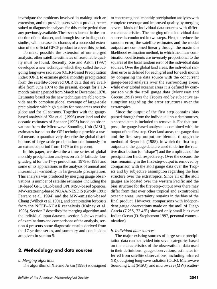
FIG. 2. Mean precipitation (mm day−1) for the period from July 1987 to May1994 from the original Spencer estimates (top), the adjusted Spencer estimates(middle), and the base product of the merged analysis of Xie and Arkin (1996)(bottom).

2544 Vol. 78, No. 11, November 1997

anic areas from 60°S to 60°N for the period from July1987 to December 1988, with estimates for Decem-ber 1987 missing. Both the NOAA/NESDIS and theChang estimates are produced using observations froma single SSM/I platform. Improvements are expectedin these estimates by using both of the available SSM/I satellites when two are available.

Since none of the observational data sources is ableto monitor precipitation with reasonable quality overmid- and high-latitude oceanic areas, precipitationdistributions produced by numerical models are in-cluded to ensure full global coverage of precipitation.The model-produced precipitation data used in thisstudy is that from the NCEP–NCAR reanalysis, whichis defined by assimilating quality-controlled observa-tions from all possible sources using the same globalmodel for the entire 40-yr period from 1957 to 1996(Kalnay et al. 1996). The monthly precipitation dataused in this study covers the entire globe and extendsfrom 1979 to 1995.

The merged analysis using the five kinds of indi-

vidual data sources described above has proved to beable to provide the distribution of precipitation for theglobe with high quality (Xie and Arkin 1996; Adleret al. 1996). However, the GPI and the SSM/I-basedestimates are not available for most of the period from1979 to mid-1987. To facilitate the extension of themerged analysis, it is necessary to find other satellite-based estimates of precipitation with extended avail-ability and reasonable quality. Although many sortsof observations are available from various meteoro-logical satellites since the beginning of the 1970s, onlythe emission data from the MSU and the OLR datafrom the Advanced Very High Resolution Radiometer(AVHRR) provide continuous temporal coverage withuseful information from which large-scale precipita-tion estimates can be made.

The MSU-based precipitation data used here arebased on the monthly estimates of Spencer (1993),which cover the global oceans from 60°S to 60°N andextend from January 1979 to May 1994. A precipita-tion index is first calculated from the anomalous tem-

FIG. 3. Global precipitation distributions (mm day−1) for August 1987 from the satellite-derived GPI, Grody, Chang, and OPI estimates.


perature elevation in MSU channel 1 (50.3 GHz),where warming is mainly due to the thermal emissionby liquid water. This index is then calibrated into rain-fall using observations from over 100 coastal and atollgauges around the globe. The spatial distribution ofthe Spencer precipitation index, however, exhibits twomajor systematic differences from estimates based onthe SSM/I and the GPI. The Pacific intertropical con-vergence zone (ITCZ) is characterized by a precipi-tation maximum over the eastern Pacific in the Spen-cer estimates, while it has its maximum over the west-ern Pacific warm pool coupled with a minimum overthe central Pacific in the GPI and most SSM/I-basedestimates (Janowiak et al. 1995; Adler et al. 1996). Inaddition, the midlatitude storm tracks are much stron-ger in the Spencer estimates than in other estimates.No conclusions regarding the relative quantitative ac-curacies of the various estimates can be made, becauseof the lack of direct precipitation measurements overthe oceanic areas in question. However, this system-

atic differences between the MSU and the othersources would result in an undesirable temporal dis-continuity in the merged analysis. Adjustments to thevarious sources are therefore needed to ensure thatartifacts in the form of spatial or temporal discontinu-ities do not degrade the utility of the merged analysis.

For that purpose, a special dataset of global monthlyprecipitation is created by merging the gauge obser-vations of the GPCC, the satellite estimates of the GPI,NOAA/NESDIS, and the Chang, and the NCEP–NCAR reanalysis for the 8-yr period from July 1987to June 1995. The merged analysis for this 8-yr pe-riod, called base product, is then used to adjust theoriginal Spencer estimates as follows. First, the meanannual cycle is calculated for both the Spencer esti-mates and the base product for each grid box usingdata for the period from July 1987 to May 1994 whenboth are available. The adjustment factor is then de-fined for each grid box and for each calendar monthas the ratio of the local mean of the base product over

FIG. 4. Global precipitation distributions (mm day−1) for August 1987 from the adjusted Spencer estimates (MSU-R), the gauge-based analysis of the GPCC, the NCEP–NCAR reanalysis, and the CMAP.

2546 Vol. 78, No. 11, November 1997

a 9 × 9 grid array centered at the target to that of theSpencer estimates, with its value limited to a range of0.5–2.0. The original Spencer estimates for the entireperiod from January 1979 to May 1994 are finallymodified month by month by multiplying with the ad-justment factor appropriate for the grid box and forthe month, resulting in the dataset, which we will re-

fer to as the MSU-R, used in this study. This processretains the temporal and spatial variability during theperiod while constraining the large-scale features ofthe Spencer estimates to match the combination of therecent data sources (Fig. 2). However, some differ-ences between the MSU-R (middle) and the base prod-uct (bottom) are found in smaller-scale features, prob-ably because of year-to-year variations in the positionof rainbands associated with the storms tracks and oce-anic convergence zones.

The other satellite estimate that is available for theentire 17-yr period is the OPI, which is based on thefindings that the anomaly of precipitation correlateswell with that of OLR over most of the globe and thatthe proportional coefficient relating them can be ex-pressed with high accuracy as a linear function of thelocal mean precipitation (Xie and Arkin 1997). TheOPI estimates monthly precipitation for a grid area inthree steps. First, the mean annual cycle of precipita-tion is obtained, and the precipitation anomaly is es-timated from the OLR anomaly using the coefficientappropriate for the mean precipitation at each locationand for each calendar month. The total precipitationis finally estimated as the sum of the mean annualcycle and the anomaly. The process requires a baseperiod for which the mean annual cycle of precipita-tion is known; in the present study, the merged analy-sis for the 8-yr base period from July 1987 to June1995 is used. The OPI estimates are available for theentire globe and for the entire 17-yr period.

c. Merged analysisA monthly precipitation analysis is then constructed

for the 17-yr period from January 1979 to December1995 by merging the seven kinds of individual datasources, whenever available, using the algorithm ofXie and Arkin (1996). For convenience, hereafter wewill call this dataset of global monthly precipitationthe CPC Merged Analysis of Precipitation (CMAP).Figures 3 and 4 show the distributions of global pre-cipitation for August 1987 from the individual datasources and from the CMAP. All of the individual datasources exhibit similar patterns of large-scale precipi-tation distribution, but with differences in smaller-scale features and in amplitudes. The GPI containslarger values over extratropical areas, and the NOAA/NESDIS, Chang, and MSU-R estimates, which arebased on fewer temporal samples, exhibit consider-able local variation, while the distributions of the GPI,OPI, and reanalysis are smoother. The merged analy-sis attempts to take advantage of each individual

FIG. 5. Distributions of the mean precipitation (top; mm day−1)for the 17-yr period from 1979 to 1995 from the CMAP using allsources and its bias (middle; mm day−1) and rms difference(bottom; mm day−1) compared to the observation-only version ofthe CMAP. Areas with more (less) precipitation observed in theobservation-only version, with differences larger than ±0.5 mmday−1, are indicated by heavy (light) shading in the bias map.


source, with patterns determinedby the combination of satelliteestimates and model outputs andamplitude defined by the gaugeobservations.

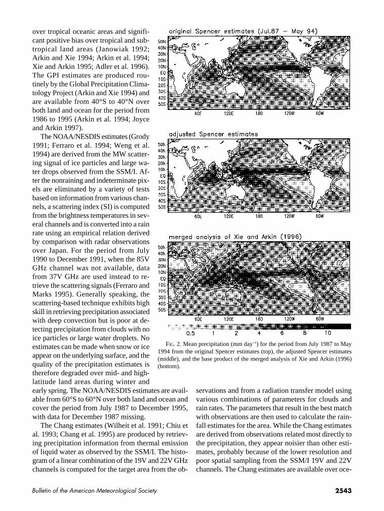
Since global precipitationdistributions are often used toverify simulations and predic-tions from numerical models ofthe atmosphere, a version of theCMAP that is based only on ob-servations, and thus can be usedfor independent comparisonswith model-based products, isrequired. At the same time,complete global fields of pre-cipitation, which are not obtain-able without the use of modelforecasts, are needed for manyother purposes, such as diagnos-tic analyses of the global hydro-logical cycle. The merging algorithm of Xie and Arkin(1996) was used to create an observation-only ver-sion of the CMAP by dropping the NCEP–NCAR re-analysis dataset and using only the six observation-based data sources. (This same process could be ap-plied to any one, or combination, of the input datasetsto create an analysis that did not use, for example, es-timates based on SSM/I observations. However, weare not aware of any pressing requirement for otherversions, and so only the “all-sources” and “observa-tion-only” versions were constructed.) The OPI andthe MSU-R are redefined by using the base productmerged from GPCC gauge data and satellite estimatesof the GPI, NOAA/NESDIS, and Chang to ensure thatthe no-model version of the merged analysis is com-pletely independent of the model results. We will re-fer to the observation-only product as the CMAP/O.To examine the differences between the two versionsof the merged analysis, comparisons are conductedbetween the CMAP and CMAP/O. Shown in Fig. 5are the mean distribution of the CMAP using allsources and its bias and rms difference relative to theCMAP/O for the 17-yr period from 1979 to 1995. Nosatellite estimates are available with reasonable qual-ity over oceanic areas poleward of 60°S/N. The larg-est differences between the CMAP and the CMAP/Oare observed in the midlatitude oceanic storm tracks,where significant differences in precipitation existbetween the satellite estimates and the reanalysis.Some differences are also found in the tropical oce-

anic convergence zones, but with substantially smallermagnitude relative to the local mean precipitation.Over land areas, the two versions of the CMAP areidentical over grid areas with one or more gauges andare very close over most other grid areas.

In addition to the monthly value of precipitation,relative error for each 2.5°lat–long grid area is esti-mated using the method described in Xie and Arkin(1996) and included in the 17-yr dataset as an indexof the quality of the merged analysis. Over the so-called anchor grid areas, where the merged analysisis defined to have the same value as that in the gauge-based analysis, the relative error is defined as the spa-tial sampling error of the gauge observations, whichis assumed to be a function of the density of the localgauge network. Over other grid areas, including alloceanic areas and land areas with no gauge coverage,the error is estimated as the expectation of the randomerror of the first-step-output, which is a linear combi-nation of several individual sources with weightsbased on the random errors of each. Xie and Arkin(1996) showed that the relative error estimated in thismanner agreed very well with that calculated by com-paring with independent observations over land areas.Over oceanic areas, where no additional data are avail-able to verify the various assumptions involved in thedefinition of the relative error, the accuracy of thisfield is less certain. More work is needed to furtherour understanding of the error structures of the indi-vidual data sources and to improve the quantitative es-

FIG. 6. Distribution of the estimated error (percentage of the mean) for the monthly analysisaveraged over the 17-yr period.

2548 Vol. 78, No. 11, November 1997

timation of the relative error of the CMAP over oce-anic areas (Oki and Sumi 1994; Huffman 1997).

Figure 6 shows the distribution of the estimatederror, relative to the mean, for monthly precipitationaveraged over the 17-yr period. Relatively small er-rors are observed over most populated land areas in

western Europe, China, and North America, whilerelatively large errors are found over desert areas andthe polar caps, where light precipitation is observedby sparse gauge networks. Over the oceans, only acrude estimate based on subjective assumptions re-garding the error structures for the individual datasources is available, and the results therefore can beonly used as indexes of the relative quality of themerged analysis. This yields a smooth field with val-ues of about 25% over the global oceanic areas from60°S to 60°N and around 30% polarward where onlyOPI and model outputs are available. Unlike the errorfields presented by Huffman et al. (1997), no contri-bution from sampling error is explicitly included here.

3. Investigation

a. Temporal continuity and spatial coherenceOne potential shortcoming of the 17-yr CMAP re-

sults from the use of different individual data sourcesfor the different periods. As shown in Fig. 1, only fourkinds of data (gauge, MSU-R, OPI, and reanalysis) areavailable during the early part of the period from Janu-ary 1979 to December 1985, while all of the seven datasources are used for the period following July 1987.In particular, the absence of the SSM/I-based esti-mates, which play an important role in defining theanalysis over global oceanic areas, might result in sig-nificant artifacts in the spatial distribution patterns andtemporal variations depicted by the dataset.

Two experiments are conducted to examine thepossible systematic differences in the spatial distribu-tions and the discontinuity in time series. First, a varia-tion of the CMAP is constructed for the period fromJuly 1987 to December 1995 by using only the gaugeobservations, OPI and MSU-R estimates, and theNCEP–NCAR reanalysis. The results are then com-pared to the version of CMAP that uses all seven datasources for the same period to investigate the impactof the estimates based on GPI and SSM/I observations.

Figure 7 shows the distribution of the mean pre-cipitation for the period as obtained from the all-sources version of the CMAP (top) and its bias(middle) and rms difference (bottom) compared to theversion without the GPI and the SSM/I-based esti-mates. No significant differences are observed overthe global land areas where precipitation distributionis determined mainly by the gauge observations. Overoceanic areas, the bias is generally very small, typi-cally less than 0.2 mm day−1, while the rms difference

FIG. 7. Distributions of the mean precipitation (top; mm day−1)for the period from July 1987 to December 1995 from the CMAPand its bias (middle; mm day−1) and rms difference (bottom; mmday−1) from the version excluding the GPI and the SSM/I-basedestimates. Areas with more (less) precipitation observed in theversion excluding the GPI (SSM/I) estimates, with differenceslarger than 0.2 mm day−1, are indicated by heavy (light) shadingin the bias map.


is about 10%–20% and exhibits a distri-bution pattern roughly similar to that ofthe total precipitation.

Figure 8 shows the time series of themean precipitation for several latitudezones over the oceans as obtained fromthe CMAP based on all available sourcesfor the entire 17-yr period (solid line) andfrom that using only the gauge observa-tions, MSU-R and OPI estimates, and theNCEP reanalysis for entire period (dot-ted line). These time series are, of course,identical until July 1987, when the SSM/I-based estimates became available. En-couragingly, no discontinuity is observedin any of the time series around July 1987when the data used changed. The time se-ries for the two versions of the mergedanalysis exhibit the same temporal varia-tion patterns with similar amplitudes overall of the seven zonal areas for the periodfrom July 1987 to December 1995. Therms difference between the two versionsof the CMAP (dashed line) is very smallover high latitudes where reanalysis,which is used in both versions, plays amajor role in determining the mergedanalysis, while moderate differences(~15%) are observed over the tropicaloceans where the GPI and SSM/I-basedestimates receive significant weights inthe merging. Not shown are the time se-ries of precipitation and differences overland areas, where the merged analysis isstrongly constrained by the gauge-basedanalysis and the changes in satellite data availabilityhave essentially no impact.

b. Comparison with independent gaugeobservationsThrough cross validation and simulation tests, Xie

and Arkin (1996) demonstrated that the merging al-gorithm used in this study is able to construct globalprecipitation analyses with better quality than the in-dividual data sources used. To investigate the quan-titative quality of the merged analysis, comparisonsare made with a nearly independent monthly rainfalldataset, which is constructed by the GPCP SurfaceReference Data Center (SRDC) by interpolatinggauge observations over several selected land areaswith much denser networks than that of the GPCC

(McNab, http://www.ncdc.noaa.gov/ogp/papers/mcnab.html).

The SRDC monthly precipitation dataset used inthis comparison covers 15 2.5°-lat–long grid areas lo-cated over five areas in Australia, Canada, Honduras,southeast United States, and Thailand, where gaugenetworks present relatively high density and uniformdistributions (see Fig. 9 of Huffman et al. 1997). Theareal mean precipitation for each grid area is calcu-lated by an algorithm called PRISM, which is basedon linear regression of gauge precipitation and terrain(Daly et al. 1994). Since the SRDC dataset is basedon observations from over 10 times as many gaugesas in the GPCC dataset and only a small portion ofthe gauges are duplicated (see Table 1 in Huffman etal. 1996), the SRDC precipitation analysis is nearly

FIG. 8. Time series of the mean precipitation (mm day−1) from the CMAP withall sources (solid line), CMAP with no GPI and SSM/I-based estimates (dottedline), and their rms difference (dashed line) over several oceanic zonal areas.

2550 Vol. 78, No. 11, November 1997

independent of the GPCC gauge-based analysis andthereby the merged analysis. Only the SRDC valuesfor grid areas with 10 or more gauges are used in thisstudy to ensure that the comparison results representthe quality of the merged analysis and not simply thesimilarity between the SRDC and GPCC datasets.

Table 1 shows the results for a 6-yr period fromJanuary 1986 to December 1991. In general, the qual-ity of the merged analysis is very good and it improveswith the increasing numbers of gauges available in theGPCC dataset. The correlation, bias, and relative ran-dom error are about 0.88, 6%, and 75% over grid ar-eas with no GPCC gauge where the merged analysisis defined by interpolating the nearby gauge data withconstraints in the “shape” of the precipitation fielddetermined by the satellite estimates and model out-puts, while they are typically over 0.9, less than 5%and 20% over grids areas with GPCC gauges where

the merged analysis is defined as thesame as the GPCC gauge analysis. Thelarge bias (123%) and random error(89%) for the grid areas with one GPCCgauge come from a grid area over Thai-land where significant inhomogeneityexists in precipitation distribution be-cause of the mountainous terrain. Inclu-sion of more gauge observations in theGPCC analysis is desirable to improvethe quality of the merged analysis oversuch areas. There are small increases inthe relative bias and random error, anddecreases in the correlation in Table 1 forgrid areas with 4, or 5 or more, stations.These fluctuations, while not clearly sta-tistically significant, appear to result from

the fact that, on average, less precipitation is observedover the grid areas with more GPCC gauges. Since thefundamental random error, or noise, in the system doesnot decrease in proportion, this results in higher relativeerror and degraded correlations for the grid areas withless precipitation. Over oceanic areas, where indepen-dent observations with reasonable spatial and tempo-ral coverage are not available, the quality of the mergedanalysis cannot be tested satisfactorily at this time.

c. Comparison with the merged analysis of Huffmanet al. (1997)The merged analysis described in this study is com-

pared to that of Huffman et al. (1997) for the periodfrom July 1987 to December 1994 when both areavailable. Since the merged analysis of Huffman et al.(1997) is produced from the gauge observations andthe satellite estimates based on the GPI and the SSM/I

observations, the observation-only(CMAP/O) version of our merged analy-sis is used in this comparison. Figure 9shows the spatial distributions of the cor-relation (top), bias (middle), and root-mean-square difference (bottom) be-tween the two datasets. Good agree-ments, characterized by high correlation,relatively small bias, and random error,are observed over global land areaswhere gauge data plays a major role inboth of the algorithms and over tropicaland subtropical oceanic areas wheremost satellite estimates exhibit highskills in estimating large-scale precipi-tation (Xie and Arkin 1995; Janowiak et

TABLE 1. Comparisons of the SRDC gauge data with the CMAP.

GPCC gauge number

0 1 2 3 4 5+

Bias (%) CMAP 6.3 88.9 −3.9 1.0 −0.5 5.1CMAP/O 5.2 88.9 −3.9 1.0 −0.5 5.1

Rmse (%) CMAP 74.6 123.9 19.5 16.8 18.3 25.1CMAP/O 75.8 123.9 19.5 16.8 18.3 25.1

Corr CMAP 0.880 0.919 0.923 0.968 0.959 0.951CMAP/O 0.876 0.919 0.923 0.968 0.959 0.951

CMAP: CPC merged analysis of precipitation with all sourcesCMAP/O: CPC merged analysis of precipitation—observation only

TABLE 2. Mean precipitation (mm day−1).

Sources Area DJF MAM JJA SON Annual

CMAP Land 1.76 1.82 2.07 1.80 1.86(All sources) Ocean 2.99 3.01 3.07 3.01 3.02

Globe 2.64 2.67 2.79 2.67 2.69

Jaeger (1976) Land 1.83 1.82 2.39 2.01 2.01Ocean 3.00 2.81 2.98 2.86 2.91Globe 2.67 2.53 2.81 2.62 2.66

Legates and Land 1.85 1.89 2.22 1.90 1.97Willmott (1990) Ocean 3.67 2.51 2.85 3.57 3.15

Globe 3.16 2.33 2.67 3.10 2.82


al. 1995). Significant differences occurover the extratropical oceans, where theanalysis of Huffman et al. (1997) is de-fined as identical to the emission-basedestimates of Chang, while, in theCMAP/O it is determined from a linearcombination of the estimates from bothSSM/I-based estimates, the MSU-R, andthe OPI, with a bias correction based onthe tropical atoll gauge observations ofMorrissey and Greene (1991) and sub-jectively derived extrapolation to theextratropics. Some differences over landareas can be attributed to the fact thatHuffman et al. (1997) correct the gauge-based analysis for systematic errorcaused by aerodynamic effects (Sevruk1989), while we used the GPCC analy-sis in its original form. The differencesobserved over the oceans, meanwhile,may come from the different sourcesused in the analysis as well as the differ-ent ways to combine them.

4. Global precipitation

The spatial and temporal variability ofglobal precipitation as observed in theCMAP is investigated for the 17-yr pe-riod from 1979 to 1995 and compared tothe long-term means of Jaeger (1976;hereafter called J76) and Legates andWillmott (1990; hereafter called LW).Figures 10–14 present the spatial distri-butions of the mean precipitation asobtained from the 17-yr CMAP (top),and from the long-term means of J76(middle) and LW (bottom) for the entireyear and for the four seasons December–February (DJF), March–May (MAM),June–August (JJA), and September–No-vember (SON), while Table 2 shows theprecipitation amounts averaged over theland, the ocean, and the entire globe.Here, the land areas are defined as those 2.5° lat–longgrid boxes with 50% or more land coverage.

In general, the 17-yr mean of the CMAP is in goodagreements with those of J76 and LW, especially overland areas. The annual mean precipitation over the en-tire globe is 2.69 mm day−1 in the 17-yr CMAP, com-

pared to 2.66/2.82 mm day−1 in J76/LW. All threedatasets exhibit similar large-scale distribution pat-terns for the annual mean precipitation (Fig. 10), withrainbands associated with the ITCZ, the South Pacificconvergence zone (SPCZ), the midlatitude oceanicstorm tracks, and the tropical continental maxima. A

FIG. 9. Correlation (top), bias (middle), and rms difference (bottom) betweenthe merged analysis of Huffman et al. (1997) and the CMAP for the period fromJuly 1987 to December 1994. Both the bias and the rms difference are plotted inpercentage relative to the CMAP.

2552 Vol. 78, No. 11, November 1997

gap in the ITCZ is observed over the central Pacificin the long-term mean of LW and, although not as dis-tinct, in the 17-yr CMAP as well, while the long-termmean of J76 exhibits broader and smoother distributionsfor the rainbands. Major differences are observed overthe eastern Pacific where only satellite-derived estimatesare available. Heavy rainfall, greater that 10 mm day−1,is observed in LW, while values in J76 are approximatelyhalf that. In CMAP, a well-defined ITCZ with peak val-ues roughly midway between J76 and LW is observed.

Significant seasonal variations in global precipita-tion are observed in the 17-yr CMAP. During DJF(Fig. 11), the SPCZ is strong and the ITCZ is relativelyweak over the central and eastern Pacific. Themidlatitude storm tracks are connected with the ITCZin the Southern Hemisphere, while they are more sepa-

FIG. 10. Distributions of the annual mean precipitation (in mmday−1) as obtained from the CMAP (top), from Jaeger (1976)(middle), and from Legates and Willmott (1990) (bottom).

FIG. 11. As in Fig. 10 except for the December–February (DJF)mean precipitation.

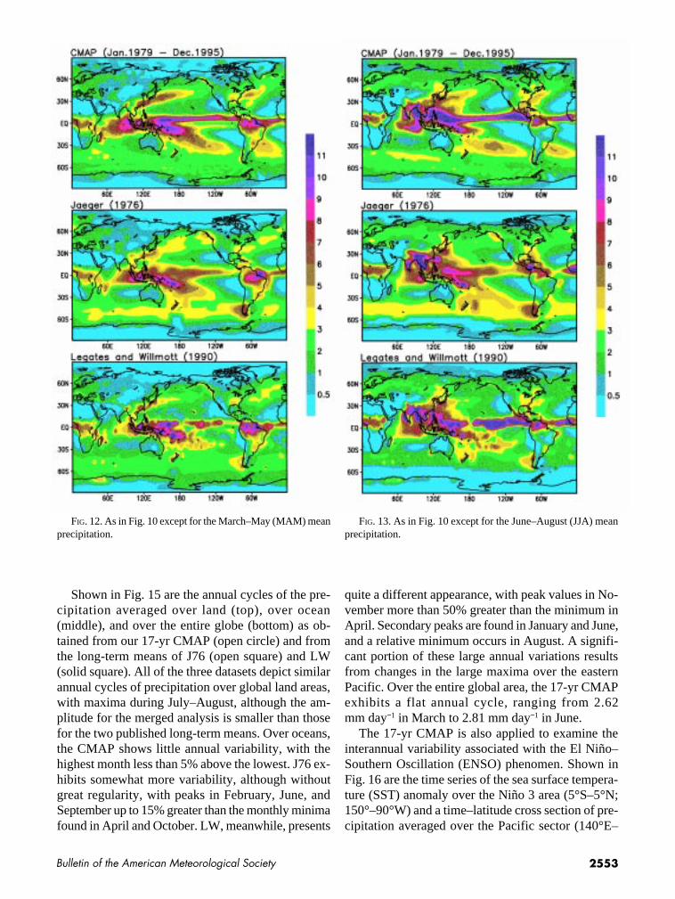
rated in the Northern Hemisphere. The SPCZ becomesweaker and the ITCZ intensifies over the western Pa-cific warm pool during MAM (Fig. 12). During JJA(Fig. 13), the SPCZ is at its weakest, while the ITCZis strong over both the eastern and western Pacific,with a slight relative minimum observed over its cen-tral part. The precipitation distribution for the SONperiod (Fig. 14) is characterized by the SPCZ recov-ering its strength and by a moderate ITCZ with largeprecipitation over the central Pacific. Similar behav-ior is observed in J76 and LW, except that the sea-sonal variations of the ITCZ over the central and east-ern Pacific are quite different in both phase and theamplitude. Generally speaking, J76 tends to exhibitsmaller precipitation for all seasons over the easternPacific, while LW gives much larger values.


Shown in Fig. 15 are the annual cycles of the pre-cipitation averaged over land (top), over ocean(middle), and over the entire globe (bottom) as ob-tained from our 17-yr CMAP (open circle) and fromthe long-term means of J76 (open square) and LW(solid square). All of the three datasets depict similarannual cycles of precipitation over global land areas,with maxima during July–August, although the am-plitude for the merged analysis is smaller than thosefor the two published long-term means. Over oceans,the CMAP shows little annual variability, with thehighest month less than 5% above the lowest. J76 ex-hibits somewhat more variability, although withoutgreat regularity, with peaks in February, June, andSeptember up to 15% greater than the monthly minimafound in April and October. LW, meanwhile, presents

quite a different appearance, with peak values in No-vember more than 50% greater than the minimum inApril. Secondary peaks are found in January and June,and a relative minimum occurs in August. A signifi-cant portion of these large annual variations resultsfrom changes in the large maxima over the easternPacific. Over the entire global area, the 17-yr CMAPexhibits a flat annual cycle, ranging from 2.62mm day−1 in March to 2.81 mm day−1 in June.

The 17-yr CMAP is also applied to examine theinterannual variability associated with the El Niño–Southern Oscillation (ENSO) phenomen. Shown inFig. 16 are the time series of the sea surface tempera-ture (SST) anomaly over the Niño 3 area (5°S–5°N;150°–90°W) and a time–latitude cross section of pre-cipitation averaged over the Pacific sector (140°E–

FIG. 12. As in Fig. 10 except for the March–May (MAM) meanprecipitation.

FIG. 13. As in Fig. 10 except for the June–August (JJA) meanprecipitation.

2554 Vol. 78, No. 11, November 1997

60°W). A significant annual cycle is observed that isclearly modified by the SST anomaly. The magnitudeof the precipitation becomes larger, and the distribu-tion extends farther south when the SST is warmerthan average, while the precipitation becomes weakerin general when the SST anomalies are negative.

Since the time–latitude cross section in Fig. 16 isnot able to reveal the east–west variation in precipita-tion, spatial distributions are composited for warm andcold ENSO episodes, and their differences are inves-tigated. Although there are many ways to define anENSO episode, we adopted a rather simple and ob-jective approach in which a cold/warm ENSO episodeis declared for a season if the SST anomaly over theNiño 3 area is < −0.5°C/> 0.5°C for the period. Theclassification based on this method results in 3–6ENSO events for each three-month period during the

17-yr period. Figure 17 shows the distributions of thedifference observed during the warm and cold condi-tions (warm minus cold) for the DJF, MAM, JJA, andSON seasons.

During DJF, warm episodes are characterized bymore precipitation over the central Pacific, southeast-ern South America, the extreme northeastern Pacificand adjacent coastal regions of North America, andover a belt extending from the eastern Pacific, acrossthe Gulf of Mexico well into the Atlantic; and by lessprecipitation over the western Pacific, the central Pa-cific away from the Tropics, Amazonia, and SouthAfrica. During MAM, in addition to the variation as-sociated with Pacific ITCZ that exhibits similar pat-terns as during DJF, the Atlantic ITCZ is more intenseand farther north than normal during warm episodes.During JJA, there is more precipitation all the wayacross the Pacific and less precipitation over most ofthe southeast Asian monsoon area during warm epi-

FIG. 14. As in Fig. 10 except for the September–November(SON) mean precipitation.

FIG. 15. Annual cycles of mean precipitation (mm day−1) overland (top), ocean (middle), and the entire globe (bottom) from the17-yr CMAP (open circle), from Jaeger (1976) (open square) andfrom Legates and Willmott (1990) (solid square).


sodes. The storm track over thenorthwestern Pacific is farthernorth than during cold episodes,bringing more precipitation overJapan and its adjacent oceanicareas during warm episodes.During SON, the SPCZ dis-placed markedly toward thenortheast relative to cold epi-sodes, and the Pacific ITCZ isagain stronger during warm con-ditions. Although based on arelatively short dataset that in-cludes only 3–6 events, the com-posite difference maps presentedhere provide us with a more spa-tially complete and systematicpicture of the ENSO-relatedinterannual variability in large-scale precipitation over theglobe than has been possible inthe past. Most variations shownhere are in general agreementwith previous studies byRopelewski and Halpert (1987,1989), which were based on his-torical station observations. However, the resultsshown in Fig. 17 enable us to see more of the full spa-tial character of the coherent ENSO-related variabil-ity over the globe, even though the short period ofrecord makes statistical significance difficult to assess.

5. Conclusions

Global monthly precipitation analyses have beenconstructed on a 2.5° lat–long grid for the 17-yr pe-riod from 1979 to 1995 by merging seven kinds of in-dividual data sources with different characteristics.These include gauge-based monthly analyses from theGlobal Precipitation Climatology Centre as well as theextension discussed by Xie et al. (1996), estimates in-ferred from a variety of satellite observations, and theprecipitation distributions from the NCEP–NCARreanalysis. Named the CPC Merged Analysis of Pre-cipitation (CMAP), the 17-yr dataset provides globalmonthly precipitation distributions with full coverageand improved quality compared to the individual datasources.

Investigation showed no apparent systematic dif-ferences in spatial distributions or discontinuities in

time series in the 17-yr dataset of the CMAP despitethe different data sources used for the different peri-ods. Verification of the CMAP with a nearly indepen-dent gauge dataset confirmed its high quality over landareas. Comparisons with the merged analysis ofHuffman et al. (1997) showed close agreement be-tween the two datasets over land and over tropical andsubtropical ocean areas, while significant differenceswere found over the extratropical oceans.

The 17-yr CMAP dataset was used to investigatethe annual and interannual variability in large-scaleprecipitation over the globe. The distributions of sea-sonal and annual mean precipitation resemble thoseobserved in the published long-term means of Jaeger(1976) and Legates and Willmott (1990) but withmajor differences over oceans, especially over theeastern Pacific. The annual global mean precipitationis 2.69 mm day−1, with values of 1.86 (3.01) over land(oceans). The interannual variability associated withthe ENSO phenomenon is similar to that found byprevious studies but with much more coherent detailover the oceans.

More work is needed to improve the quality of theCMAP and to further extend its temporal coverage.Since the final quality of the merged analysis is pri-

FIG. 16. Time series of the SST anomaly over the Niño 3 area (5°S–5°N; 150°–90°W)(top) and the time–latitude diagram for the precipitation (in mm day−1) averaged over thePacific section from 140° to 60°W (bottom).

2556 Vol. 78, No. 11, November 1997

marily determined by the quality of the input datasources, improvements of the individual data sourcesare essential, especially over mid- and high latitudeswhere no observation-based data sources provide cov-erage with reasonable quality. The accurate definitionof the bias and error structures for the individual datasources is the key to the success of the merged analy-sis. At present, this is based largely on subjective as-sumptions, particularly over the oceans. Further workis necessary to improve our quantitative understand-ing of the individual error structures. Particularly, therelationship among the error for various individualdata sources must be investigated and included in thedefinition of the linear combination coefficients usedin the maximum likelihood estimation. The observa-tions to be made available from the TRMM project

(Simpson et al. 1988) will certainly be crucial in solv-ing this problem, at least for the Tropics and subtrop-ics. Finally, since some applications in meteorologyand hydrology require higher resolution in space andtime, development of a global precipitation datasetwith finer resolution is under consideration.

Acknowledgments. The authors would like to express theirthanks to C. Ropelewski and J. Janowiak of the Climate Predic-tion Center and A. Gruber of the National Environmental Satel-lite, Data and Information Service of NOAA for invaluable dis-cussions throughout this research. Comments by Dr. GeorgeHoffman, Professor Mark Morrissey, and R. Ferraro were veryhelpful in improving our original manuscript. Readers interestedin the dataset described in this paper may contact the first authorfor its availability and updated information.

FIG. 17. Differences between warm and cold ENSO episodes during the 17-yr period from 1979 to 1995 for DJF, MAM, JJA, andSON precipitation. Areas wetter (drier) during warm ENSO episodes, with differences larger than 0.5 mm day−1, are indicated byheavy (light) shading.


References

Adler, R. F., A. J. Negri, P. R. Keehn, and I. M. Hakkarinen, 1993:Estimation of monthly rainfall over Japan and surroundingwaters from a combination of low-orbit microwave and geo-synchronous IR data. J. Appl. Meteor., 32, 335–356.

——, G. J. Huffman, and P. R. Keehn, 1994: Global rain estimatesfrom microwave adjusted geosynchronous IR data. RemoteSens. Rev., 11, 125–152.

——, C. Kidd, M. Goodman, G. Petty, and M. Morrissey, 1996:PIP-3 intercomparison results. PIP-3 Workshop, College Park,MD, NASA, 20 pp.

Arkin, P. A., 1979: The relationship between fractional coverageof high cloud and rainfall accumulations during GATE overthe B-scale array. Mon. Wea. Rev., 107, 1382–1387.

——, and B. N. Meisner, 1987: The relationship between large-scale convective rainfall and cold cloud over the western hemi-sphere during 1982–84. Mon. Wea. Rev., 115, 51–74.

——, and P. E. Ardanuy, 1989: Estimating climatic-scale precipi-tation from space: A review. J. Climate, 2, 1229–1238.

——, and P. Xie, 1994: The Global Precipitation ClimatologyProject: First Algorithm Intercomparison Project. Bull. Amer.Meteor. Soc., 75, 401–419.

——, R. Joyce, and J. E. Janowiak, 1994: IR techniques: GOESPrecipitation Index. Remote Sens. Rev., 11, 107–124.

Arpe, K., 1991: The hydrological cycle in the ECMWF short-rangeforecasts. Dyn. Atmos. Oceans, 16, 33–60.

Barrett, E. C., and D. W. Martin, 1981: The Use of Satellite Datain Rainfall Monitoring. Academic Press, 340 pp.

Chang, A. T., L. S. Chiu, and G. Yang, 1995: Diurnal cycles ofoceanic precipitation from SSM/I data. Mon. Wea. Rev., 123,3371–3380.

Chiu, L. S., A. Chang, and J. E. Janowiak, 1993: Comparison ofmonthly rain rates derived from GPI and SSM/I using prob-ability distribution functions. J. Appl. Meteor., 32, 323–334.

Daly, C., R. P. Neilson, and D. L. Phillips, 1994: A statistical-topographic model for mapping climatological precipitationover mountainous terrain. J. Appl. Meteor., 33, 140–158.

Dodge, J., 1994: The WetNet Project. Remote Sens. Rev., 11,5–21.

Ferraro, R. R., N. C. Grody, and G. F. Marks, 1994: Effects ofsurface conditions on rain identification using SSM/I. RemoteSens. Rev., 11, 195–209.

——, and G. F. Marks, 1995: The development of SSM/I rain rateretrieval algorithms using ground-based radar measurements.J. Atmos. Oceanic Technol., 12, 755–770.

Gates, W. L., 1992: The Atmospheric-Model IntercomparisonProject. Bull. Amer. Meteor. Soc., 73, 1962–1970.

Grody, N. C., 1991: Classification of snow cover and precipita-tion using the Special Sensor Microwave Imager. J. Geophys.Res., 96, 7423–7435.

Huffman, G. J., 1997: Simple estimates of root-mean-square ran-dom error for finite samples of estimated precipitation. J. Appl.Meteor., in press.

——, G. J., R. F. Adler, B. R. Rudolf, U. Schneider, and P. R.Keehn, 1995: Global precipitation estimates based on a tech-nique for combining satellite-based estimates, rain gauge analy-sis, and NWP model precipitation information. J. Climate, 8,1284–1295.

——, and Coauthors, 1996: The Global Precipitation Climatol-ogy Project (GPCP) combined precipitation dataset. Bull.Amer. Meteor. Soc., 77, 5–20.

Jaeger, L., 1976: Monatskarten des Niederschiags fur die ganzeErde. Berichte des Deutscher Wetterdienstes, Offenbach, 33pp. and plates.

Janowiak, J. E., 1992: Tropical rainfall: A comparison of satellitederived rainfall estimates with model precipitation forecasts,climatologies, and observations. Mon. Wea. Rev., 120, 448–462.

——, P. A. Arkin, P. Xie, M. L. Morrissey, and D. R. Legates,1995: An examination of the east Pacific ITCZ rainfall distri-bution. J. Climate, 8, 2810–2823.

Joyce, R., and P. A. Arkin, 1997: Improved estimates of tropicaland subtropical precipitation using the GOES PrecipitationIndex. J. Atmos. Oceanic Technol., 14, 997–1011.

Kalnay, E., and Coauthors, 1996: The NCEP/NCAR 40-year Re-analysis Project. Bull. Amer. Meteor. Soc., 77, 437–472.

Legates, D. R., and C. J. Willmott, 1990: Mean seasonal and spa-tial variability in gauge corrected global precipitation. Int. J.Climatol., 10, 111–127.

Morrissey, M. L., and X. Greene, 1991: The Pacific atoll raingagedata set. Tech. Rep. Univ. Hawaii, Manoa, Honolulu, Hawaii.

Oki, R., and A. Sumi, 1994: Sampling simulation of TRMM rain-fall estimation using radar-AMeDAS composites. J. Appl.Meteor., 33, 1597–1608.

Reynolds, R. W., 1988: A real-time global sea surface tempera-ture analysis. J. Climate, 1, 75–86.

Richards, F., and P. A. Arkin, 1981: On the relationship betweensatellite-observed cloud cover and precipitation. Mon. Wea.Rev., 109, 1081–1093.

Ropelewski, C. F., and M. S. Halpert, 1987: Global and regionalscale precipitation patterns associated with El Niño/SouthernOscillation. Mon. Wea. Rev., 115, 1606–1626.

——, and ——, 1989: Precipitation patterns associated with highindex phase of the Southern Oscillation. J. Climate, 2, 268–284.

——, J. E. Janowiak, and M. S. Halpert, 1985: The analysis anddisplay of real time surface climate data. Mon. Wea. Rev., 113,1101–1106.

Rudolf, B., H. Hauschild, W. Rueth, and U. Schneider, 1994:Terrestrial precipitation analysis: Operational method and re-quired density of point measurements. NATO ASI Series, 126,173–186.

Schubert, S., R. Rood, and J. Pfaendtner, 1993: An assimilateddataset for earth sciences applications. Bull. Amer. Meteor.Soc., 74, 2331–2342.

Sevruk, B., 1989: Reliability of precipitation measurements. Proc.WMO/IAHS/ETH Workshop on Precipitation Measurements,St. Moritz, Switzerland, WMO, 13–19.

Shepard, D., 1968: A two-dimensional interpolation function forirregularly spaced data. 23rd Natl. Conf. of American Com-puting Machinery, Princeton, NJ.

Simpson, J., R. F. Adler, and G. R. North, 1988: A proposed tropi-cal rainfall measuring mission. Bull. Amer. Meteor. Soc., 69,278–295.

Spencer, R. W., 1993: Global Oceanic precipitation from the MSUduring 1979-91 and comparisons to other climatologies. J.Climate, 6, 1301–1326.

2558 Vol. 78, No. 11, November 1997

Vose, R. S., R. L. Schmoyer, P. M. Steurer, T. C. Peterson, R.Heim, T. R. Karl, and J. K. Eischeid, 1992: The Global His-torical Climatology Network: Long-term monthly temperature,precipitation, sea-level pressure, and station pressure data.Rep. ORNL/CDIAC-53, Carbon Dioxide Inf. Anal. Cent., OakRidge Natl. Lab., Oak Ridge, TN, 25 pp. [Available from Car-bon Dioxide Information Analysis Center, Oak Ridge NationalLaboratory, Oak Ridge, TN 37831-6335.]

Weng, F.-Z., R. Ferraro, and N. Grody, 1994: Global precipita-tion evaluation using Defense Meteorological Satellite ProgramF10 and F11 Special Sensor Microwave Imager (SSM/I). J.Geophys. Res., 99, 25 535–25 551.

Wilheit, T. J., A. T. C. Chang, and L. S. Chiu, 1991: Retrieval ofthe monthly rainfall indices from microwave radiometric mea-surements using probability distribution functions. J. Atmos.Oceanic Technol., 8, 118–136.

World Climate Research Programme, 1993: Global observations,analyses and simulation of precipitation. Rep. WCRP-78,WMO/TD 544, World Meteor. Org., Geneva, XX pp.

Xie, P., and P. A. Arkin, 1995: An intercomparison of gauge ob-servations and satellite estimates of monthly precipitation. J.Appl. Meteor., 34, 1143–1160.

——, and ——, 1996: Analyses of global monthly precipitationusing gauge observations, satellite estimates, and numericalmodel predictions. J. Climate, 9, 840–858.

——, and ——, 1997: Global monthly precipitation estimatesfrom satellite-observed Outgoing Longwave Radiation. J. Cli-mate, in press.

——, B. Rudolf, U. Schneider, and P. A. Arkin, 1996: Gauge-based monthly analysis of global land precipitation from 1971–1994. J. Geophys. Res., 101(D14), 19 023–19 034.

global precipitation: a 17-year monthly analysis based on ...zli/meto620/readings for aosc424... ·...

Documents