Globalization, Acquisitions and Endogenous Firm Structure

Larry D. Qiu and Wen Zhou∗

The University of Hong Kong

April 20, 2009

Abstract

A model of heterogeneous firms with multiple products and endogenous firm structure is developedto investigate how firms respond to trade liberalization. Firm-level productivity is endogenized as firmsacquire capital through mergers and acquisitions to reach optimal product scope (number of products)and capital scale (the amount of capital in each plant). The analysis shows that while more efficientfirms produce more products, plant and firm level capital have an inverse U-shaped relationship withfirm efficiency. A firm responds to different types of trade liberalization differently, leading to differentredistribution of capital and productivity. In an importing country that opens to trade unilaterally, capitalmoves from high efficiency firms to low efficiency firms, and firm and industry productivity increase.Under bilateral trade liberalization, capital moves from low efficiency firms to high efficiency firms, andproductivity may increase or decrease. The analysis highlights the importance of resource reallocationafter trade liberalization and the linkage between product and acquisition markets.

Keywords: firm heterogeneity, trade liberalization, mergers and acquisitions, scale, scope, multi-product, firm structure

JEL Code: F12, F13, F15, L11, L25

1 Introduction

Drastic trade liberalization, unilateral, bilateral or multilateral, has been implemented in many places in theworld as part of the globalization process. Traditional international economics has primarily been concerned

∗Correspondance: larryqiu@hku.hk and wzhou@business.hku.hk. We thank Jiahua Che, Jee-Hyeong Park, Wing Suen,Shangjin Wei and seminar participants at the Chinese University of Hong Kong, Fudan University, the Hong Kong Universityof Science and Technology, Seoul National University, the University of Hong Kong and the 2008 International Industrial Organi-zation Conference for their helpful comments.

1

about patterns of and gains from trade, but more recent studies have shifted the focus to how heterogenousfirms respond to trade liberalization differently and how industry productivity changes through firm entryand exit.1 The present study follows this trend and goes beyond by endogenizing firm-level productivity andby emphasizing the interaction between product and factor markets.

The majority of the new studies follows Melitz’s (2003) model, which assumes that every firm producesa single product.2 The reality is clearly very different. According to Bernard, Jensen and Schott (2005) andBernard, Redding and Schott (2008), 41 percent of U.S. manufacturing firms produce more than a singleproduct, and these firms account for 91 percent of U.S. manufacturing output and 95 percent of U.S. exports.3

When firms produce multiple products, they can respond to trade liberalization by changing the number oftheir products (i.e., product scope) as well as by the entry/exit and output adjustment that have been thefocus of previous research. Investigating how heterogeneous firms change their product scope differentlyis in itself an interesting question. Furthermore, this extra channel of adjustment through product scopemay affect responses in other channels and ultimately affect industry productivity. A few researchers, mostnotably Bernard, Redding and Schott (2009) and Nocke and Yeaple (2006), have already realized the need tostudy multiproduct firms. This study was designed with the distinctive feature that product scope and plantlevel productivity were both endogenized. Unlike the work of Bernard, Redding and Schott (2009) withexogenous plant productivity, the productivity was endogenized by allowing firms to acquire a productiveresource called capital. Unlike Nocke and Yeaple (2006) who imposed a tradeoff between product scopeand plant productivity, we allow the two variables to be chosen independently.

For firms to be able to adjust their productivity through changes in capital, there must be a channelthrough which capital moves across and within firms. The trading of capital was modelled as mergers andacquisitions (M&As) in an acquisition market. M&A is a major method of industrial restructuring (UNC-TAD, 2000) and the quickest and least costly way to respond to external shocks such as trade liberalization.4

Waves of mergers have been documented as a consequence of trade liberalization and other industry shocks(Mitchell and Mulherin, 1996). Breinlich (2008) found that the Canada-United States Free Trade Agree-ment of 1989 increased domestic Canadian M&A activity by over 70%. Using data on Swedish firms for theperiod 1980-1996, Greenaway, Gullstrand and Kneller (2008) have shown that intensified international com-petition caused more M&As. M&A is particularly relevant to multiproduct firms, as acquisition is the mosteffective way to add new products quickly. In the context of firm heterogeneity, it would be interesting to in-vestigate how firms behave differently in the acquisition market, i.e., who buys capital and who sells capital,in response to trade liberalization. Firms’ endogenous adjustment of product lines through M&A will alsoaffect other decisions including product scope, and thus ultimately affect industry productivity. Breinlich(2008), for example, found that resources were transferred from low efficiency firms to high efficiency firms

1Bernard and Jensen (1999), Pavcnik (2002), Melitz (2003), Trefler (2004). See the survey by Helpman (2006).2Another pioneer study is that of Bernard, Eaton, Jensen and Kortum (2003), who also focus on single-product firms.3The calculation is based on U.S. manufacturing and trade data from 1972 to 1997. Products are defined by five-digit Standard

Industrial Classification categories.4According to the United Nations’ World Investment Report (UNCTAD, 2000), worldwide M&As grew at an annual rate of 42

percent over the period 1980-1999 to reach US$2.3 trillion in 1999. More than 24,000 M&As took place during that period, andthe value of M&As relative to world GDP rose from 0.3 percent in 1980 to 2 percent in 1990 and to 8 percent in 1999.

2

through M&As following the Canada-United States Free Trade Agreement.M&A is not simply another channel through which firms respond to exogenous shocks. It highlights

the important linkage between product and factor markets, which has not been thoroughly investigated inthe literature. Trade liberalization is usually considered to affect firm behavior through either the productmarket or the factor (labor) market, but not both. Melitz and Ottaviano (2008) assume exogenous wage rateand focused only on the competition in the product market. Melitz (2003) and Bernard, Redding and Schott(2009) derive product demand from CES preferences, and in their model trade liberalization works its effectmainly through changes in the labor market. Although the trading of capital in the present study seems towork in a way similar to the labor market, there are two important differences between labor and capital.First, unlike labor, capital affects both firm-level and plant-level productivity. Second, trade liberalizationaffects both product and acquisition markets, which permits investigating the linkage between the two. Theresult are very different from those obtained when the two markets are considered separately.

Consider first a closed economy in which a continuum of firms produce differentiated products. Firmsare distinguished by their intrinsic efficiency and may choose to produce multiple products. The marginalproduction cost of any product is assumed to be decreasing in both the firm’s intrinsic efficiency and theamount of capital allocated to the product. Capital is acquired in a perfectly competitive acquisition marketbefore firms produce and compete in a monopolistically competitive product market. We will show thatwhile more efficient firms maintain larger product scope (number of varieties), they do not necessarilypossess larger size (capital at the firm level) or scale (capital at the plant level). In fact, size and scale areinversely U-shaped in intrinsic efficiency. An efficient firm sells its products at a relatively low price. Furtherreducing marginal production cost by increasing capital will not bring much extra benefit. As a result, anincrease in efficiency may induce a firm to decrease its capital stock. Nevertheless, more efficient firmsalways produce more at the plant and firm level. Thus, this model helps reconciling seemingly conflictingpredictions of previous studies. On the one hand, scope and plant-level output are positively correlated,confirming the theoretical and empirical findings by Bernard, Redding and Schott (2008, 2009). On theother hand, scope and firm-level size (measured by capital) may be negatively correlated, confirming theprediction of Nocke and Yeaple (2006).

Trade liberalization brings both opportunities (of exporting) and challenges (through increased com-petition from imports), and the two often have opposite effects. To isolate these effects, we consider twotypes of trade liberalization: unilateral and bilateral. Under unilateral trade liberalization in the industryconcerned, firms in the importing country face more competition in the product market. They all try todownsize, pushing down the price of capital. Facing reduced profitability in the product market and reducedcapital prices in the acquisition market, firms respond differently. Because they are efficient in using capital,high efficiency firms are mainly affected by changes in the product market, and they end up selling capi-tal. Low efficiency firms, by contrast, are less responsive to the product market and are affected mainly bychanges in the acquisition market. They will buy capital. Low efficiency firms expand their scope, whilehigh efficiency firms reduce scope. The total number of varieties produced by home firms is reduced. Aseach plant expands scale and reduces output, firm- and industry-level productivity improve.

Under bilateral trade liberalization in the industry concerned, the effects of increased opportunity and

3

increased competition are both present. Interestingly, it turns out that when the two countries are symmetric,the effect of increased opportunity dominates and, as a result, capital moves from low efficiency firms tomore efficient ones. Low efficiency firms reduce scope while high efficiency firms expand their scope. Thetotal number of varieties consumed in each country increases. The impact on productivity is nonethelessambiguous. When products are close substitutes, productivity tends to rise; when products are very differ-entiated, productivity tends to drop. Although we focused on two symmetric countries, the analysis can beeasily extended to bilateral trade liberalization between two or more asymmetric countries.

Our model predicts that firm size (measured by capital or output) is distributed more evenly in theimporting country under unilateral trade liberalization, and more skewed under bilateral trade liberalization.This helps explain another set of conflicting predictions. Bernard, Redding and Schott (2009) showed thatsize distribution is more skewed after trade liberalization, while Nocke and Yeaple (2006) showed thatthe distribution should be less skewed. It now appears that both are possible depending on the type ofliberalization or the relative size of the two countries.5

Thus, by endogenizing firm structure through choices of scope and scale, and by introducing an acqui-sition market for the trading of capital, this study highlights M&A as an important channel through whichfirms respond to trade liberalization. It demonstrates a new source of productivity improvement throughresource reallocation, and highlights the linkage between product and acquisition markets. The implicationsare, first, that productivity adjusts not only at the industry and firm level, but also at the individual prod-uct level through the redistribution of capital across and within firms. Such a redistribution of productiveresources within an industry is at the heart of industrial dynamics in the face of exogenous shocks. Its im-pact on industry and firm productivity are stronger and more direct than the reallocation of output, whichhas been the focus of previous studies. A second implication is that the linkage between the product andacquisition markets cannot be ignored. Changes in the product market always induce an offsetting changein the acquisition market. Trade liberalization may reduce capital prices so much that capital moves fromhigh efficiency firms to low efficiency firms, yet firm and industry productivity increases, a result impossiblewhen the two markets are considered separately.

These findings relate to three strands of prior work. Most relevant is the international trade literatureon heterogenous firms, where most studies (see the survey by Helpman, 2006) assume single-product firmsand predict that industry productivity improves as a result of the exit of the least efficient firms (e.g., Melitz,2003), i.e., through inter-firm output reallocation. Bustos (2007) extended Melitz’s (2003) model by al-lowing firms to upgrade their technologies at some extra fixed cost. Recent models of multiproduct firms(e.g., Baldwin and Gu, 2005; Eckel and Neary, 2005; Bernard, Redding and Schott, 2009, 2008; Nocke andYeaple, 2006; Feenstra and Ma, 2007) have emphasized intra-firm output reallocation as a new source ofproductivity improvement. For example, Bernard, Redding and Schott (2009) start with the premise thatproductivity differs not only across firms but also among different products produced by the same firm.

5Bernard, Redding and Schott (2006) and Nocke and Yeaple (2006) reached their conclusions considering symmetric bilateraltrade liberalization. Although in the model considered here, bilateral trade liberalization leads unambiguously to more skewedsize distribution, this result obtains when the two countries are symmetric. If the two countries are asymmetric, it is reasonable toconjecture that depending on the parameters, either force may dominate and the size distribution may be more or less skewed.

4

They showed that each firm responds to trade liberalization by dropping its least efficient products. Whilethey relied on output reallocation with fixed plant-level productivity, this study has emphasized resourcereallocation with endogenous productivity. Nocke and Yeaple (2006) imposed an exogenous tradeoff be-tween product scope and firm-level productivity and predicted that trade liberalization would induce highefficiency firms to shrink their product lines and low efficiency firms to expand product lines. In contrast,this study considered productivity adjustment at the plant level as independent of the choice of productscope. The modeling of M&As enabled us not only to generate within-firm rationalization through produc-tivity and product scope adjustment, but also to reconcile the conflicting predictions of these prior studies.Furthermore, most previous formulations have relied on either the product market (Melitz, 2003; Nocke andYeaple, 2006) or the factor market (Bernard, Redding and Schott, 2009; Melitz and Ottaviano, 2008) inexplaining how trade liberalization affects firm choices. This study considered both markets.

This study is also relevant to M&A in an international context,6 particularly how trade liberalizationaffects firms’ merger incentives. Long and Vousden (1995) have shown that while unilateral tariff reductiondiscourages cost-reducing mergers, bilateral tariff reductions have the opposite effect. Long and Vousdenfocused solely on M&A incentives, but this study has examined how heterogenous firms adjust their capitalscale and product scope through M&A in response to trade liberalization. Moreover, like many others,Long and Vousden emphasized strategic effects in an oligopoly setting. This study assumed a perfectlycompetitive acquisition market. Spearot (2008) used the same cost function and two-stage game consideredhere, but assumed single-product firms and capital transactions in single units. His conclusion that onlymoderately efficient firms acquire capital was thus very different. Several empirical studies have found thattrade liberalization can trigger merger waves (Mitchell and Mulherin, 1996; Breinlich, 2008; Greenaway,Gullstrand and Kneller, 2008). This work provides theoretical support for those findings.

Finally, it might be pointed out that this work is remotely related to industrial organization studies ofendogenous product scope, which emphasize strategic effects (Brander and Eaton, 1984; Shaked and Sutton,1990; and Johnson and Myatt, 2003). Since our purpose was to study how heterogeneous firms respond totrade liberalization by changing their firm structure, strategic effects were excluded by assuming that firmsbuy and sell capital in a perfectly competitive acquisition market.7

6In this study, mergers were endogenous in the sense that all merger opportunities have been exhausted in the original equilib-rium and only an exogenous shock to the the economy such as trade liberalization can trigger new mergers. Elsewhere we havestudied endogenous mergers between heterogenous firms producing single and homogeneous products (Qiu and Zhou, 2007). Thefocus of that study was how mergers alter the incentives for subsequent mergers and why mergers occur in waves.

7Lommerud and Sorgard (1997) have shown that mergers may change a firm’s optimal choice of product scope. They did notconsider the impacts of trade liberalization.

5

2 Closed Economy

2.1 The model

Consider a closed economy with a numeraire good and a differentiated goods industry. Production of thenumeraire good displays constant returns to scale and requires two units of labor for one unit of output.Hence, wage rate, w, is equal to 1

2 in the economy. In the differentiated goods industry, there are a continuumof firms. Each firm draws its efficiency level, a, from a uniform distribution on [0, 1]. The parameter a, whichis the only exogenous characteristic that distinguishes firms, is called a firm’s intrinsic efficiency. A larger adenotes more efficient production.

A firm can maintain multiple plants, each producing a single variety. In doing so, it incurs a managementcost, mv2, where m > 0 and v is the number of varieties that the firm produces. The cost of producing eachvariety is derived from a constant-returns-to-scale technology q = (axl)

12 , in which x is capital input and l

is labor input. In the short run when its capital is fixed, the variable cost isminl(wl) subject to q = (axl)12 .

The minimum cost is waxq

2. Since w = 12 , this yields the cost function for the variety as

c(q|a, x) = q2

2ax.

This cost function has been widely used in industrial organization studies of M&As (e.g., Perry and Porter,1985).

The production technology in this model displays decreasing returns to (output) scale: marginal produc-tion cost, q

ax , increases with q. This cost structure ensures interior solutions for optimal quantity at arbitrarylevels of capital, which is particularly convenient in a model where capital is endogenous. While it simpli-fies the calculation greatly, the assumption is not crucial. The major results hold even if marginal costs areconstant, an assumption commonly used in models of international trade.

Given the above description, we note that the reciprocal of average production cost, i.e., qc =

2axq , is

the plant-level labor productivity. Industry-level labor productivity is defined similarly as the reciprocal ofindustry average cost, i.e., industry aggregate quantity divided by aggregate cost.8 Labor productivity thusincreases with both the intrinsic efficiency, which is exogenous, and the amount of capital allocated to eachplant, which is endogenous. While a is the intrinsic efficiency for a firm, ax represents the productionefficiency of a particular variety.

In previous models of heterogeneous firms with single factor (labor), there is no difference betweena firm’s intrinsic efficiency, a, and its labor productivity. In models of single-product firms, firm levelproductivity has been fixed.9 In Bernard, Redding and Schott’s (2009) model of multiple-product firms,

8Thus, in discussing productivity, management costmv2 will be ignored to focus on the costs directly incurred in the productionprocess.

9The only exception is the work of Bustos (2007), who allowed single-product firms to upgrade their technology (i.e., a pro-portional reduction of marginal costs) at some additional fixed cost, giving rise to endogenized plant level productivity. She found

6

although the firm-level average productivity was endogenous, plant level productivity was still fixed. Nockeand Yeaple (2006) endogenized plant level productivity, but they imposed an exogenous tradeoff betweenproductivity and product scope. In this model, by contrast, product scope and plant level productivity areboth endogenized, and the two choices are independent. Although there is a tradeoff between scale andscope within a firm, the tradeoff disappears when firms can freely buy capital in the acquisition market. Forexample, a firm may buy capital to increase scope and scale at the same time. In this sense, firm structure istruly endogenized in this model.

Each firm is endowed with one unit of capital. With this endowment and the knowledge of their intrinsicefficiencies, firms play a two-stage game. In the first stage (the acquisition stage), firms buy and sell capitalin a perfectly competitive acquisition market (as in Jovanovic and Rousseau, 2002). If a firm sells all ofits capital, it becomes inactive in the product market, i.e., it exits the production. An inactive firm stillkeeps its a and may choose to re-enter the product market later by buying capital from the acquisitionmarket. Entry and exit incurs no extra cost. After the trading of capital, every firm which still possessespositive capital chooses its number of varieties and the allocation of capital into each plant. A firm’s choiceof structure therefore consists of its product scope (the number of varieties), plant-level capital scale (theamount of capital used in each plant), and consequently firm-level capital size (total amount of capital). Forexpositional convenience, scale, scope and size will be treated as continuous variables. Moreover, capital isassumed perfectly divisible, and there is no minimum capital requirement for running a plant. In the secondstage (the production stage), all existing firms (i.e., those who did not exit) produce and sell their productsin a product market characterized by monopolistic competition.

In this model, capital represents industry-specific physical assets that are needed in production. Unlikefinancial assets, capital must be acquired through M&As rather than from financial institutions. Unlikevariable inputs such as labor, capital are fixed inputs in production (in the short run), such as the distributionnetwork, machinery and production capacity. Capital is thus a productive resource that directly determinesproduction efficiency. We assume that a firm can acquire capital only from the acquisition market (i.e.,only from other firms), which implies that the supply of capital in the industry is perfectly inelastic. Suchan assumption is justified if the total amount of such physical assets cannot be increased within a shorttime. It is important to point out, however, that the results still hold even if new capital can be generated inresponse to a capital price increase. By assuming a perfectly competitive acquisition market, we imply thatcapital is homogeneous and acquisition is partial. That is, instead of acquiring a stand-alone target firm, theacquirer buys some productive assets from other firms and use them along with its own assets. As arguedby Jovanovic and Rousseua (2002), transactions in such a used-capital market work just like those in anM&A market. Maksimovic and Phillips (2001) report that about half of U.S. M&A transactions are partial

that a reduction in variable trade cost induces more firms to upgrade and more firms to self-select into the export market. Whiletechnology upgrading is binary and irreversible (no possibility for downgrading), capital flow is continuous and can increase ordecrease. More importantly, technology supply is perfectly elastic; there is no competition for the technology (the fixed cost ofupgrading does not change when more firms try to upgrade). In contrast, there is competition for capital: When firms try to producemore in response to trade liberalization, they demand more capital, pushing up the capital price. Thus, capital is best regarded asa rare productive resource in limited supply, and trade liberalization changes both the benefit and cost of acquiring capital, both ofwhich are at the heart of the model.

7

acquisitions or divestitures by multi-product conglomerates.The model will now be analyzed backwards, first the product market, then the acquisition market, and

finally the industry equilibrium.

2.2 The product market

Assume L identical consumers in the economy. To analyze competition in the product market, we followMelitz and Ottaviano (2008) to assume that the representative consumer has a quasi-linear preference overa numeraire good and all varieties in the industry concerned:

U = Q0 + α

Zi∈Ω

qidi−1

2β

µZi∈Ω

qidi

¶2− 12γ

Zi∈Ω

q2i di,

where Q0 is the consumption of the numeraire good, Ω is the set of all product varieties, qi is the consump-tion of variety i, α (> 0) and β (> 0) capture the substitution between the industry’s products and thenumeraire, and γ (> 0) represents the degree of product differentiation between varieties.10

Consumers maximize their utility subject to budget constraints. Utility maximization yields the inversedemand function for variety i:

pi = A− bqi, where A =αγ

βM + γ+

β

βM + γP and b =

γ

L. (1)

In this demand function, pi is the price of variety i, M is the measure of Ω, and P =Ri∈Ω pidi is the aggre-

gate price of all varieties. The vertical intercept A of the demand function summarizes the competitivenessof the product market: If more products compete in the market, the demand for each product will drop,representing cannibalization. Compared with CES preferences which give rise to constant and exogenousmarkups, the quasi-linear preference used in this model leads to variable markups that are more consistentwith empirical evidence (Helpman, 2006). More importantly, it allows capturing the competition effects inboth the product and acquisition markets, and thus investigation of the linkage between them. Althoughlinear demand is highly specific, it is no more specific than constant elasticity demands that had been usedin most studies. More importantly, our results hold as long as elasticities are not constant.

As firms engage in monopolistic competition, each firm takes A as given when it chooses its output. Iffirm a (i.e., a firm whose intrinsic efficiency is a) uses xi amount of capital to produce variety i, its chooses

10In the demand for any particular product, the cross coefficient is β while the own coefficient is β+γ. As γ decreases, varietiesare less differentiated. In the limiting case of γ = 0, the industry’s varieties become perfect substitutes.

8

output qi to maximize its profit from this variety:11

maxqi≥0

πi ≡ (A− bqi)qi −q2i2axi

. (2)

The resulting quantity, price and profit for this variety are, respectively,

qi(xi) =axiA

2abxi + 1, pi(xi) =

(abxi + 1)A

2abxi + 1, and πi(xi) =

axiA2

2(2abxi + 1). (3)

Greater demand (i.e., a larger A) leads to more output, a higher price and more profit for each variety. Asthe variety’s production efficiency, axi, increases, the output and profit are larger but the price is lower.

Since a variety’s profit, πi(xi), is increasing and concave in xi, a firm will always allocate its total capitalamong its varieties equally. Consequently, the subscript i can be dropped in (3), and firm level productivityalways equals plant level productivity.

2.3 The acquisition market

Let R be the market price of capital. If a firm chooses scope v and scale x, its capital cost is (vx − 1)R,where vx − 1 is the firm’s net demand for capital, which can be negative (meaning that the firm is sellingcapital). Thus, the firm’s optimization problem in the acquisition market is

maxx≥0,v≥0

Π(v, x) ≡ vπ(x)− (vx− 1)R−mv2 = vπ(x) +R−mv2,

where π(x) ≡ π(x)−xR is the firm’s profit from each single plant, taking into consideration the capital costbut not the management cost. It is as if the firm first sells its endowment of a unit of capital in the acquisitionmarket and then chooses how much capital to buy for each of its plant. Since there is no transaction cost,selling and buying capital is fully reversible.

Given the above decomposition of the profit function, the firm’s optimization problem can be solved intwo steps: The optimal scale is x∗ = argmaxx π(x), which is independent of the value of v, and the optimalscope is then v∗ = argmaxv Π(v, x∗).

11Thus, we assume away the cannibalization effect that a firm’s output in one variety has on the profitability of its other varieties.As shown by Schwartz and Thompson (1986) and Baye, Crocker and Ju (1996), in an effort to gain market share from competingcompanies or forestall entry, many companies instruct their divisions to act as independent firms despite the apparent cannibalizationeffect. If our assumption is relaxed to accommodate the cannibalization effect, our major conclusions still hold, as demonstrated byFeenstra and Ma (2007) in a setting similar to Melitz (2003) with the addition of the cannibalization effect.

9

2.3.1 Scale

Definey ≡ A√

2R. (4)

In the acquisition market, firms treat A, R, and consequently y as given. Since π(x) is proportional to A2

2 ,y2 = A2

2R represents the value of expanding capital relative to the capital price.>From the first-order condition (the second-order condition is always satisfied), ∂π

∂x = 0, we obtain theoptimal scale for each plant:

x∗ =

⎧⎪⎪⎨⎪⎪⎩0 for a ≤ a0,

y√a−12ab for a > a0,

(5)

where a0 ≡ 1y2

. Later we will show that in equilibrium, y > 1 and therefore a0 < 1. (5) shows that veryinefficient firms will not operate in the product market (their holding of capital is zero). Intuitively, when a

is small, the optimal firm scale is small. Each firm’s profit from the product market will also be small, andselling all its capital (i.e., exiting the industry) gives the firm a better payoff. The least efficient firms exitthe product market because they can realize higher profits from the acquisition market.12

For firms that hold positive amount of capital, (5) says that plant scale depends on y, which is someratio between A and R. Thus, firms’ demand for capital depends on both the product market and theacquisition market. In previous models, trade liberalization affected firm choices through either the productmarket (Melitz and Ottaviano, 2008; Nocke and Yeaple, 2006) or the factor market (Melitz, 2003; Bernard,Redding and Schott, 2009). In this model, however, the impact of trade liberalization works through bothmarkets, and the linkage between the two (as all changes in the acquisition market are induced by changes inthe product market) becomes crucial. Note that scale depends only on y, the ratio between A and R, ratherthan on their individual values, and it increases with y. This is easy to understand: The marginal benefit ofexpanding scale (i.e., acquiring capital) is proportional to A2

2 , while the marginal cost of acquiring capitalis R. The optimal scale balances marginal benefit with marginal cost and therefore should increase whenA2

2R increases. As a result, a higher demand in the product market or a lower price in the acquisition marketallows firms to expand plant scale. It also allows firms with lower efficiency to remain active (i.e., a0 islower).

Only sufficiently efficient firms hold capital. However, firms with higher intrinsic efficiency do not

12Most studies follow Melitz (2003) to assume fixed production cost for the least efficient firms to exit. Without assuming fixedcost, Melitz and Ottaviano (2008) obtain exit when the constant marginal costs that some firms draw are higher than the interceptof a linear demand function. In our model, demand is linear as in Melitz and Ottaviano (2008) and there is no fixed production cost.A firm’s marginal cost can be arbitraily small (when its output is close to zero) even if it is very inefficient. It will always generatesome profit, however small, in the product market. Thus, a firm exits only because it can sell its capital in the acquisition market.

10

necessarily have larger plant scale, as

∂x∗

∂a=2− y

√a

4a2b

⎧⎪⎪⎨⎪⎪⎩> 0 for a ∈ (a0, 4a0),

< 0 for a > 4a0.

When 4a0 < 1, capital scale increases with the firm’s intrinsic efficiency when the efficiency is low, anddecreases with efficiency when the efficiency is high, an inverse U-shaped relationship. The intuition isthe following. Although the marginal returns from capital (∂π∂x ) are always positive, the magnitude of themarginal return depends on a firm’s intrinsic efficiency. Note that ∂2π

∂a∂x =A2(1−2abx)2(2abx+1)3

. When a is small,the production efficiency ax is small; each variety is sold at a high price, where demand is highly elastic.Increasing x allows the firm to lower its price. Since demand is very elastic, lowering price brings a largebenefit. By contrast, when a is large, the marginal production cost is low; each variety is already sold atlow price, where the demand is barely elastic. Increasing x still allows the firm to lower its price, but theextra benefit is small because demand is not very elastic. Thus, the marginal benefit of expanding scale isinversely U-shaped in a, which translates into an inverse U-behavior of optimal scale in a, as the marginalcost of expanding scale is fixed.

Although firms with higher intrinsic efficiency (a) may have smaller capital scale (x∗), they still havehigher production efficiency, as ax∗ = y

√a−12b increases with a. This monotonicity ensures that more-

efficient firms produce more:

q∗ =A

2b

µ1− 1

y√a

¶and thus ∂q∗

∂a > 0. Furthermore, plant and firm level productivity, which is

q

c=

r2a

R,

also increases with a.

2.3.2 Scope

Given the optimal scale, a firm’s profit from each variety (after paying for capital) is

π(x∗) =

⎧⎪⎪⎨⎪⎪⎩0 for a ≤ a0,

R(y√a−1)22ab for a > a0,

(6)

11

which is strictly increasing in a for a > a0. Given π(x∗), the first-order condition for optimal scope (thesecond-order condition is always satisfied), ∂Π

∂v = π(x∗)− 2mv = 0, leads to v∗ = π(x∗)2m or

v∗ =

⎧⎪⎪⎨⎪⎪⎩0 for a ≤ a0,

R(y√a−1)2

4abm for a > a0.

(7)

Notice that∂v∗

∂a> 0 for all a > a0.

Thus, more-efficient firms have larger scope. The optimal scope balances the marginal benefit from addinga variety, which equals π(x∗), with the additional cost, which is 2vm. Since the marginal benefit increaseswith a, the optimal scope should be larger when a is higher.

Since both q∗ and v∗ are increasing in a, q∗ and v∗ are positively correlated. This confirms that intensivemargins (i.e., each variety’s output) and extensive margins (i.e., the number of varieties) are positivelycorrelated (Bernard, Redding and Schott, 2009).13 The driving force behind the correlation is the sameas that discussed by Bernard, Redding and Schott: The monotonic change of production efficiency withintrinsic efficiency. However, plant-level production efficiency is endogenous in this model but not in theirs.

2.3.3 Size

We now turn to a firm’s capital size, x∗v∗. Since x∗v∗ = 0 for a ≤ a0, the least efficient firms will notoperate in the industry. For those firms remaining,

∂x∗v∗

∂a=

R(y√a− 1)2

16a3b2m(4− y

√a)

⎧⎪⎪⎨⎪⎪⎩> 0 for a < 16a0,

< 0 for a > 16a0.

The relationship between firm size and intrinsic efficiency is jointly shaped by the properties of scale andscope. Although scope increases with a, scale is inversely U-shaped. As a result, firm size is also inverselyU-shaped.14 Note that the turning point for size (at 16a0) is larger than that for scale (at 4a0). Nevertheless,the important message is that more efficient firms do not necessarily require more capital. Also note that theenvelope theorem predicts that a firm’s profit still increases with a even though its capital size may not.

The relationship between a firm’s intrinsic efficiency and its scale, scope, size and profit is summarized

13In contrast, Nocke and Yeaple (2006) predicted a negative correlation because they assumed a negative relationship betweenplant-level marginal cost and product scope.

14Spearot’s (2008) model also suggested an inverse U-relationship between firm capital and efficiency.

12

in the following proposition.

Proposition 1. A firm’s optimal scale and size increase in its intrinsic efficiency a when a is small, but maydecrease in a when a is large. A firm’s optimal scope and profit, however, always increase in a.

Turn now to the acquisition market to determine the equilibrium R for a given A. Market clearingrequires total capital supply to equal capital demand at the industry level. Since each firm is initially endowed

with one unit of capital, the total capital supply in the industry isZ 1

01da = 1. The total capital demand is

k ≡Z 1

a0

x∗v∗da =R

8b2mρ,

whereρ ≡

Z 1

a0

(y√a− 1)3a2

da = 2y3 + 3y2(1− 2 ln(y))− 6y + 1.

Lemma 1. Given A, there exists a unique equilibrium capital price R∗ and correspondingly a unique y∗.Moreover,

dR∗

dA> 0 and

dy∗

dA< 0. (8)

Proof. See the Appendix.

At this point, A has been regarded as an exogenous variable, although later A will be solved from theproduct market equilibrium condition (1). Given A, R and the corresponding y are uniquely determined.Lemma 1 says that R∗ increases with A. That is, when demand is higher, capital will be more expensive;when demand is lower, capital will be cheaper. Thus, any change in the product market will induce a changein the acquisition market that always has an offsetting effect on firm profitability: When the product marketbecomes more profitable, capital price changes will reduce that profitability.

In previous models of heterogeneous firms, trade liberalization has affected firm profitability throughintensified competition in either the product market or the factor market, but never both. When the con-sumers’ utility function leads to cannibalization as in models of Melitz and Ottaviano (2008) and Nockeand Yeaple (2006), trade liberalization intensifies competition in the product market, but any response inthe factor market has been assumed away. When a CES utility function is used, as by Melitz (2003) and byBernard, Redding and Schott (2009), there is no cannibalization. Trade liberalization intensifies competitionin the factor market because the demand for production input (i.e., labor) increases as firms try to producemore for the export market. This model adopts the utility function used by Melitz and Ottaviano (2008),so the product market becomes more competitive after trade liberalization. At the same time, firms demandmore capital as they try to produce for the export market, pushing up the capital price. So trade liberalizationaffects firm choices through both the product market and the acquisition market. As will become evident

13

when we analyze unilateral trade liberalization, incorporating both markets into a coherent model is not asimple combination of the two effects. Rather, it leads to important conclusions that cannot be found whenthe two effects are analyzed separately.

To proceed further, we need to express the equilibrium capital price as a function of y. From the equi-librium condition, k(R∗) = 1,

R∗(y) =8b2m

ρ(y). (9)

Note that this expression is not the reduced form solution for R, as y is defined on R.

2.4 Industry equilibrium

We now turn to the equilibrium in both acquisition and product markets (i.e., to determine the equilibriumA and R). The measure of varieties is

M(y) ≡Z 1

a0

v∗da =R

4bmψ =

2bψ

ρ, (10)

where the last equality has made use of expression (9), and

ψ ≡Z 1

a0

(y√a− 1)2a

da = y2 − 4y + 3 + 2 ln(y) withdψ

dy> 0 and

d(ψρ )

dy< 0.

Substituting the optimal scale x∗ into (3) yields the equilibrium price for individual products (a firmcharges the same price for all its varieties):

p =A

2y

µ1 +

1

y√a

¶

for all a > a0. The aggregate price is therefore

P (y) ≡Z 1

a0

v∗pda =AR

8bm

φ

y=4b2√mφ

ρ32

, (11)

whereφ ≡ y3 − 2y2 − 2 + 3y − 2y ln(y) and

dφ

dy> 0.

14

By the definition of A in (1) and using (10) and (11), we have

A∗ =αγ + βP

βM + γ=

α

1 + βL

ηyρ

, where η ≡ 2yψ − φ = y3 − 6y2 + 2 + 3y + 6y ln(y). (12)

The three equilibrium values A∗, R∗ and y∗ are jointly determined by equations (4), (9) and (12). Using(9) and (12) in (4) yields the following equation expressed in y only:

Z(y) = 0, where Z(y) ≡ ρ3³yρ+ β

Lη´2 − 16b2mα2

. (13)

It can be shown that Z 0(y) > 0, Z(1) < 0, and Z(y) > 0 when y is sufficiently large. Therefore, thereexists a unique y∗ > 1 satisfying (13). Once y∗ is determined, R∗ is determined from (9) and subsequentlyA∗ is determined from (4) or (12). As a result,

Proposition 2. There exist unique equilibrium A∗ and R∗ in the closed economy.

3 Unilateral Trade Liberalization

Assume two identical countries, home and foreign, which initially do not trade with each other. The closedeconomy equilibrium in each country is as analyzed in Section 2. Now consider trade liberalization, whichpresents firms with both opportunities (of exporting) and challenges (of increased competition from im-ports). To better understand the two forces, we first study them in isolation by analyzing unilateral tradeliberalization. Specifically, we consider the following scenario: There is free trade between the two coun-tries in the numeraire good. In the differentiated goods industry, the home country opens up to imports butit cannot export to the foreign country. We will investigate in the next section the combined effect when acountry can both import and export the differentiated goods. In order to isolate the effects of trade liberal-ization, we exclude the possibility of cross-border M&A.15 Moreover, assume no variable or fixed cost oftrade. It will be clear by the end of this section that the results do not rely on these simplifications of tradecosts. Finally, trade is always balanced through the move of the numeraire good, and hence we skip thebalanced trade condition in the following analysis.

15Thus, any change in the acquisition market is induced by a change in the product market.

15

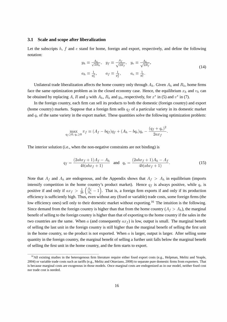
3.1 Scale and scope after liberalization

Let the subscripts h, f and e stand for home, foreign and export, respectively, and define the followingnotation:

yh ≡ Ah√2Rh

, yf ≡ Af√2Rf

, ye ≡ Ah√2Rf

,

ah ≡ 1y2h

, af ≡ 1y2f, ae ≡ 1

y2e.

(14)

Unilateral trade liberalization affects the home country only through Ah. Given Ah and Rh, home firmsface the same optimization problem as in the closed economy case. Hence, the equilibrium xh and vh canbe obtained by replacing A, R and y with Ah, Rh and yh, respectively, for x∗ in (5) and v∗ in (7).

In the foreign country, each firm can sell its products to both the domestic (foreign country) and export(home country) markets. Suppose that a foreign firm sells qf of a particular variety in its domestic marketand qe of the same variety in the export market. These quantities solve the following optimization problem:

maxqf≥0, qe≥0

πf ≡ (Af − bqf )qf + (Ah − bqe)qe −(qf + qe)

2

2axf.

The interior solution (i.e., when the non-negative constraints are not binding) is

qf =(2abxf + 1)Af −Ah

4b(abxf + 1)and qe =

(2abxf + 1)Ah −Af

4b(abxf + 1). (15)

Note that Af and Ah are endogenous, and the Appendix shows that Af > Ah in equilibrium (importsintensify competition in the home country’s product market). Hence qf is always positive, while qe ispositive if and only if axf > 1

2b

³AfAh− 1´

. That is, a foreign firm exports if and only if its productionefficiency is sufficiently high. Thus, even without any (fixed or variable) trade costs, some foreign firms (thelow efficiency ones) sell only to their domestic market without exporting.16 The intuition is the following.Since demand from the foreign country is higher than that from the home country (Af > Ah), the marginalbenefit of selling to the foreign country is higher than that of exporting to the home country if the sales in thetwo countries are the same. When a (and consequently axf ) is low, output is small. The marginal benefitof selling the last unit in the foreign country is still higher than the marginal benefit of selling the first unitin the home country, so the product is not exported. When a is larger, output is larger. After selling somequantity in the foreign country, the marginal benefit of selling a further unit falls below the marginal benefitof selling the first unit in the home country, and the firm starts to export.

16All existing studies in the heterogenous firm literature require either fixed export costs (e.g., Helpman, Melitz and Yeaple,2004) or variable trade costs such as tariffs (e.g., Melitz and Ottaviano, 2008) to separate pure domestic firms from exporters. Thatis because marginal costs are exogenous in those models. Once marginal costs are endogenized as in our model, neither fixed costnor trade cost is needed.

16

So a foreign firm with efficiency a sells in both markets if xf > 12ab

³Af

Ah− 1´

, and the sales in the twomarkets are given by (15). The corresponding prices and a variety’s total profit in the two markets are

pe =Ah(2abxf + 3) +Af

4(abxf + 1), pf =

Af (2abxf + 3) +Ah

4(abxf + 1),

πf =2abxf (A

2h +A2f ) + (Ah −Af )

2

8b(abxf + 1).

If xf ≤ 12ab

³Af

Ah− 1´

, then qe = 0. The firm makes its choices as if there were no exporting opportunity,and the results are the same as in a closed economy:

qf =Afaxf2abxf + 1

, pf =Af (abxf + 1)

2abxf + 1, and πf =

A2faxf

2(2abxf + 1).

Each plant’s profit net of capital cost is πf = πf−xfRf , where πf is given above depending on whetheror not xf > 1

2ab

³Af

Ah− 1´

. The firm chooses xf to maximize πf , which yields

xf =

⎧⎪⎪⎪⎪⎪⎪⎨⎪⎪⎪⎪⎪⎪⎩0, if a ≤ af ,

yf√a−1

2ab , if af < a ≤ ae,

yf√a−1

2ab + ye√a−1

2ab , if a > ae,

(16)

where yf , ye, af , and ae are given by (14). Note that af < ae because Af > Ah. For a ∈ (af , ae], the firmfocuses on the domestic market, so its optimal scale is determined in the same way as in the closed economy(i.e., replacing y with yf in (5)). For a > ae, the firm serves both markets and its optimal scale is the sumof the optima for serving the two markets separately.

Given this optimal scale, a firm chooses its scope, vf , to maximize its profit vf πf −mv2f + Rf . Theoptimal choice is

vf =

⎧⎪⎪⎪⎪⎪⎪⎨⎪⎪⎪⎪⎪⎪⎩0, if a ≤ af ,

Rf(yf√a−1)2

4abm , if af < a ≤ ae,

Rf (yf√a−1)2+(ye

√a−1)2

4abm , if a > ae.

Thus, the additive rule also applies to scope: When a firm serves both markets, its optimal scope is thesum of the scope optimal for serving the domestic market alone and the scope for serving the export market

17

alone.Given the optimal scale, a foreign firm’s domestic sales (in the foreign country) are qf =

Af2b

³1− 1

yf√a

´and the corresponding price is pf =

Af2

³1 + 1

yf√a

´for a > af . Its export sales (in the home country) are

qe =Af

2b

³yeyf− 1

yf√a

´and the corresponding price is pe =

Af

2

³yeyf+ 1

yf√a

´for a > ae. The firm’s pro-

ductivity isq

2aRf

for a > af . Thus, exporters are more efficient in production, produce more and earn morethan firms that produce only for the domestic market, confirming well-established empirical findings.

3.2 Industry equilibrium

To solve for the industry equilibrium, use fi to denote f(yi) for i = h, f, e. In the home country, given Ah,the acquisition market equilibrium is derived in exactly the same way as in the closed economy case. Hence,as in (9), there exists a unique capital price that satisfies

Rh =8b2m

ρh. (17)

Let Mh be the measure of all home varieties and Me be the measure of all imported varieties. Then (makinguse of Rf in (18)),

Mh(yh) ≡Z 1

ah

vhda =2bψh

ρh,

Me(yf , ye) ≡Z 1

ae

vfda =2b[ψf + ψe − ψ]

ρf + ρe + 2ρ,

where ψ(yf , ye) =

Z ae

af

(yf√a−1)2

a da > 0 and ρ = 1 + 2yeyf − y2f + 2y2e + (ye + yf )(yfye − 3) −

2 ln(ye)(y2e + 4yeyf + y2f ).

Substituting a firm’s optimal scale in its equilibrium price and making use of AhAf

= yeyf

, we obtain

ph =Ah2

³1 + 1

yh√a

´for a ≥ ah in the home country and pe =

Ah2

³1 + 1

ye√a

´for a ≥ ae in the foreign

country. The aggregate price in the home market is the sum of the prices of all products, both home-madeand imported:

Ph(yf , ye) ≡Z 1

ah

vhphda+

Z 1

ae

vfpeda =4b2√mφh

(ρh)32

+

Z 1

ae

vfpeda.

In the foreign country, given capital price Rf and using the optimal scale and scope derived earlier, we

18

obtain (see the Appendix) the total capital demand

kf ≡Z 1

0xfvfda =

Rf

8b2m(ρf + ρe + 2ρ).

>From kf = 1 we obtain

Rf =8b2m

ρf + ρe + 2ρ. (18)

The total product varieties is

Mf (yf , ye) ≡Z 1

af

vfda =2b(ψf + ψe)

ρf + ρe + 2ρ.

Using xf from (16) and the fact that AhAf

= yeyf

, we obtain the individual product price sold in the foreign

market: pf =Af2

³1 + 1

yf√a

´for a ∈ (af , 1]. Thus, the aggregate price is

Pf (yf , ye) =

Z 1

af

vfpfda

=4b2√m

(ρf + ρe + 2ρ)32

∙φf +

Z 1

ae

(ye√a− 1)2(yf

√a+ 1)

a√a

da

¸.

Finally, by definition, Ah and Af are jointly determined by

Ah =αγ + βPh

β(Mh +Me) + γ, (19)

Af =αγ + βPfβMf + γ

. (20)

Having expressed Rh and Rf as functions of yf , ye and yh (from (17) and (18)), we have five unknowns,Af , Ah, yf , ye and yh, and five equations, (19), (20) and the definitions of yf , ye and yh (from (14)), whichjointly determine the equilibrium.

3.3 Equilibrium comparison

Although the calculation has involved quite a few steps and variables, the mechanism is very clear. Whenthe home country opens to imports, foreign firms start to sell their products in the home country but homefirms are unable to export because the liberalization is unilateral. Such an import shock affects home firms’

19

a aa

scale scope size

Figure 1: Impacts of Unilateral Trade Liberalization on Firm Structure

output and consequently their capital scale and product scope. These changes in firm structure lead to somefirms selling capital and some others buying, which in turn affects the home country’s product market. Firmand industry productivity change. The following proposition summarizes the direction of the change in theimporting country.

Proposition 3. After unilateral trade liberalization, the home (importing) country undergoes the followingchanges as compared to the closed economy equilibrium:

(1) markets: the product market becomes more competitive (Ah < A∗) and capital prices drop (Rh <

R∗);(2) firm structure:

(i) capital moves from high efficiency firms to low efficiency firms: there exists ash ∈ (a∗0, 1) suchthat xhvh > x∗v∗ for a < ash and xhvh < x∗v∗ for a > ash;

(ii) all existing firms expand scale: xh > x∗ for all a ≥ a∗0;(iii) low efficiency firms expand their scope while high efficiency firms reduce their scope: there

exists avh ∈ (a∗0, 1) such that vh > v∗ for a < avh and vh < v∗ for a > avh;

(3) aggregate scope: the total number of varieties produced by home firms decreases (Mh < M∗);(4) productivity: firm and industry labor productivity improves.

Proof. See the Appendix.

The change in firm structure is shown in Figure 1, where the solid lines represent the situation beforeliberalization and the dotted lines represent the situation after liberalization. When a country opens itselfto trade, the initial change is an influx of foreign products, which immediately reduces Ah in the homecountry (a negative demand shock). The increased competition (or equivalently lower demand for any

20

particular product) lowers every home firm’s profit, which is proportional to A2h. If the capital price does notchange, every firm will adjust its structure by reducing both scale and scope (as shown in (5) and (7)), whichgenerates excess supply of capital in the industry. Rh must then drop until the acquisition market clears.The question is, at the new capital price, which firms will increase their capital and which will decrease.

Both Ah and Rh drop, and Rh must drop more so that yh rises (i.e., yh > y∗). To see this, note thatx∗h =

yh√a−1

2ab and v∗h =Rh(yh

√a−1)2

4abm ; that is, scale is increasing in yh, and scope is increasing in both yh andRh. If yh also drops, every firm will reduce both scale and scope, and the acquisition market cannot clear.But because capital is cheaper relative to demand (yh increases), every plant expands scale. The question iswhich firms sell capital (and thus must reduce their scope). Recall that a firm’s profit in the product marketincreases with its intrinsic efficiency. A change in the product market thus affects high efficiency firmsmore heavily than it affects those that are less efficient. Facing reduced product demand (which reduces thedemand for capital) and lower capital prices (which raises the demand for capital), more efficient firms willbe affected mainly by the lower product demand. As a result, their demand for capital will decrease andthey will sell capital and reduce their scope. By contrast, less efficient firms will be affected mainly by thelower capital price and they will buy capital and expand their scope. The total number of product varietiesproduced by home firms decreases. Note that the total number of varieties consumed by home consumers islikely to increase, as they consume both domestic products and imports.

All plants increase their scale, which implies that some plants originally not in the market now findit optimal to buy some capital and re-enter (the result ah < a∗0 is in the proof of the proposition). Suchentries will be at the lower end of the efficiency spectrum. That trade liberalization may induce entry bylow efficiency firms is a surprising but logical result. In the importing country, the influx of imports reducesthe demand for home products (Ah drops), which in turn reduces the capital price (Rh drops). Becauselow efficiency firms are mainly affected by changes in the acquisition market, they buy capital and re-enter.Obviously, this result relies on the linkage between the product market and the acquisition market, a featureabsent in all previous models. This analysis has shown that the response in the factor market tends to offsetthe change in the product market, and may even outweigh it so that unilateral trade liberalization inducesthe entry of low efficiency firms rather than their exit.17

The big picture is that resources (capital) move from more-efficient to less-efficient firms, which leads toa more even distribution of firm size in terms of capitalization.18 Measured by output, firm size is also dis-tributed more evenly after trade liberalization. Despite the seemingly inefficient redistribution of resourcesbetween firms, labor productivity still increases. At the firm level, every firm expands the scale of eachplant, and every product’s output is reduced due to the intensified competition. Both changes lower average

17One must be cautious in comparing this result with empirical findings such as exit by less efficient firms after Chile opened totrade unilaterally in 1970s and 1980s (Pavcnik, 2002). Our result is obtained in a partial equilibrium framework, where the lowerdemand for capital in this industry reduces capital price, while the Chile case is obviously an effect of general equilibrium with thepossible flow of extra capital to other industries.

18This direction of resource reallocation is opposite to empirical findings by Breinlich (2008) about how Canadian firms re-sponded to the Canada-United States Free Trade Agreement (CUSFTA). The CUSFTA is a bilateral trade liberalization, while theresults in Proposition 3 obtain under unilateral trade liberalization, which has not been tested empirically. The next section willshow that resource reallocation under bilateral trade liberalization is consistent with Breinlich’s finding.

21

production cost and therefore raise labor productivity.19 At the industry level, two factors oppose the im-provement of labor productivity: high efficiency firms reduce their product scope while low efficiency firmsincrease their product scope, and new entrants have lower TFP than all existing firms. Since industry pro-ductivity is the average of firm-level productivity weighted by scope, industry productivity performs worsethan firm productivity. Nevertheless, firms’ productivity improves so much that industry productivity alsoincreases.20

So competition from imports forces home firms to rationalize resources so that labor productivity in-creases, which is hardly surprising. Nevertheless, it is surprising that productivity improves in the absenceof export opportunities and as resources move from high efficiency to low efficiency firms. In models withfixed plant-level productivity, any change in industry productivity must be through entry/exit and output real-location. There is no way that industry productivity can improve when resources move from high efficiencyto low efficiency firms. In this model, trading capital and plant-level scale (which determines plant-level andfirm-level productivity) are two separate variables, although they are connected. Despite the unfavorablemovement of capital across firms, all plants increase scale, which is the driving force for labor productivityimprovements.

In the foreign country, analytical comparisons are intractable,21 but numerical calculations confirm theintuition that almost every change is the opposite of what happens in the home country. Capital becomesmore expensive. The least efficient firms exit. High efficiency firms buy capital and increase their scopewhile low efficiency firms sell capital and reduce scope, leading to a more skewed distribution of firm sizemeasured by capital or output. Every firm reduces scale. Firm and industry labor productivity decrease. Theonly change that is similar to the home country is that the product market in the foreign country also becomesmore competitive (Af < A∗) even though the foreign country does not face any competition from imports.Note that what matters for the change in the acquisition market is profitability in the product market, whereloosely speaking the total demand is Af +Ah, not Af .

4 Bilateral Trade Liberalization

Trade liberalization brings producers greater opportunities (for exporting) and greater competition (fromimported products). The previous section investigated unilateral trade liberalization where only one effect ispresent in a country. This section will examine the combined effects of bilateral trade liberalization where

19If marginal costs are constant with output, the effect of reduced output will disappear, but the effect of increased scale will stillbe present and the result will continue to hold.

20An indication of the dominance can be obtained by comparing the productivity of the least efficient firm before and after tradeliberalization. Although firm ah has lower intrinsic efficiency than firm a∗0, the former’s productivity is higher due to increasedcapital scale: c(a∗0)

q(a∗0)= R∗

2a∗0= A∗

2. Similarly c(ah)

q(ah)= Ah

2. As a result, c(ah)

q(ah)<

c(a∗0)q(a∗0)

.21In the home country, although there are no closed-form solutions, analytical comparisons are possible because the expressions

for scale and scope are exactly the same as in the closed economy, and we can prove that yh > y∗ because (19) and (12) differonly by an extra term. In the foreign country, by contrast, the expressions for scale and scope are different from those in the closedeconomy, and the expressions contain yf and ye that cannot be easily compared with y∗.

22

everything is the same except that home firms in the differentiated goods industry can now export to theforeign country.

4.1 Equilibrium after bilateral trade liberalization

Since the two countries are symmetrical, there must be a symmetric equilibrium, which we focus on. Con-sider the home country. Define

yt ≡At√2Rt

and at ≡1

y2t

where the subscript t stands for bilateral trade. Given At, a firm chooses the quantity of each variety it willproduce for both markets, qt, to maximize its combined profit from both product markets for the variety:

maxqt≥0

πt ≡ 2(At − bqt)qt −(2qt)

2

2axt. (21)

The optimal output, price and profit are, respectively,

qt =axtAt

2(abxt + 1), pt =

(abxt + 2)At

2(abxt + 1), and πt =

axtA2t

2(abxt + 1).

Given capital priceRt, the firm chooses its optimal scale for each plant to maximize the plant-level profitπt = πt − xtRt. The solution is

xt =

⎧⎪⎪⎨⎪⎪⎩0, if a ≤ at,

yt√a−1ab , if a > at.

(22)

The firm chooses its scope, vt, to maximize its total profit vtπt(xt) − mv2t + Rt, yielding the followingoptimal scope

vt =

⎧⎪⎪⎨⎪⎪⎩0, if a ≤ at,

Rt(yt√a−1)2

2abm , if a > at.

(23)

With this firm structure, the total capital demand kt ≡Z 1

0xtvtda =

Rt2b2m

ρt. A unique acquisition

market equilibrium is then determined by kt(Rt) = 1, or

Rt(yt) =2b2m

ρt. (24)

23

The aggregate variety supplied by firms in a country is Mt(yt) =

Z 1

at

vtda =bψtρt, and there are 2Mt

varieties in each country’s product market. The aggregate price is Pt(yt) = 2Z 1

at

vtptda =2b2√mφt

(ρt)32

.

By definition, At is determined by

At(yt) =αγ + βPt2βMt + γ

=α

1 + βL

ηtytρt

. (25)

Equations (24) and (25) and the definitions of yt jointly determine the three unknowns At, Rt and yt as theequilibrium in bilateral trade liberalization.

In fact, instead of going through these steps, there is an alternative and much simpler way to obtain theequilibrium. Note that the plant’s maximization problem (21) can be rewritten as

maxqt

πt =

∙At −

b

2(2qt)

¸(2qt)−

(2qt)2

2axt.

If we replace (2qt) with q, the problem is identical to that in the closed economy case, (2), except thatthe demand slope is b

2 instead of b. In other words, if in the closed economy we have equilibrium so-lutions p(A, a, x, b), q(A, a, x, b) and π(A, a, x, b), then under bilateral trade, the solutions will be pt =

p(A, a, x, b2), qt =12q(A, a, x,

b2) and πt = π(A, a, x, b2). It is straightforward to reach the following con-

clusion: if y∗(b), A∗(b) and R∗(b) are the equilibria in the closed economy, then the bilateral trade equilibriaare yt = y∗

¡b2

¢, At = A∗

¡b2

¢, and Rt = R∗

¡b2

¢.

These two approaches are not only mathematically equivalent, but also economically isomorphic. With-out any trade cost, a firm views the two product markets (domestic and export) as identical. At the sametime, a consumer is assumed not to treat domestic varieties differently from imported varieties. Comparedto the closed economy, therefore, a firm’s demand under bilateral trade is doubled (population increasesfrom L to 2L), which is captured by the change of the slope from b to b

2 (because b = γL ). From the firm’s

point of view, for given A and R, the change in the slope of the demand curve is the only difference be-tween the closed economy and bilateral trade, so its optimal scale and scope are doubled after bilateral tradeliberalization. Of course, A, R and consequently y will be different from those in the closed economy.

Since the acquisition market is not international, the change in the slope of the demand curve does notaffect the acquisition market directly, but it does so indirectly through changes in each firm’s optimal scaleand scope. This explains why Rt in (24) is obtained simply by replacing b with b

2 from R∗ in (9). Notethat the demand intercept, A, is not affected by the population size L, or b, directly. Also note that inaddition to substituting b with b

2 to get the bilateral trade equilibrium, the domestic market’s total varietiesunder bilateral trade are twice those produced by the domestic firms, and the aggregate price is also doubled.These two observations allow us to map the equilibrium condition for A∗ in (12) to that for At in (25).

24

4.2 Equilibrium comparison

We have seen how home firms respond to unilateral trade liberalization. Their responses to bilateral liber-alization can be rather different, because they now have the opportunity to export their products, which inturn affects their optimal scale and scope.

Using (5) and (22), a firm expands its scale, i.e., xt(a) > x∗(a), if and only if

(2yt − y∗)√a > 1. (26)

Similarly, we can obtain (see Appendix) conditions for vt(a) > v∗(a) and xt(a)vt(a) > x∗(a)v∗(a). In theAppendix we prove that yt < y∗ and so at > a∗0. These comparisons allow us to establish the followingproposition about the impacts of bilateral trade liberalization.

Proposition 4. After bilateral trade liberalization,(1) markets: the demand in each country drops but the combined demand in the two countries increases

(At ∈ (A∗

2 , A∗)); capital prices may increase or decrease;

(2) exit: the least efficient firms exit (at > a∗0);(3) firm structure:

(i) capital moves from low efficiency to more efficient firms: there exists as ∈ (at, 1) such thatxtvt < x∗v∗ for a ∈ (at, as) and xtvt > x∗v∗ for a ∈ (as, 1];

(ii) high efficiency firms expand while less efficient firms reduce their scale: there exists an ax ∈(at, 1] such that xt < x∗ for a ∈ (at, ax) and xt > x∗ for a ∈ (ax, 1];

(iii) high efficiency firms expand their scope while low efficiency firms reduce their scope: thereexists an av ∈ (at, 1] such that vt < v∗ for a ∈ (at, av) and vt > v∗ for a ∈ (av, 1].

(4) aggregate scope: the total number of varieties consumed in each country increases (2Mt > M∗);(5) productivity: if the capital price increases, firm-level labor productivity decreases; if the capital

price declines, firm-level and industry-level labor productivity increase.Proof: See the Appendix.

Note that as < 1 (there must be some firms which buy capital) because some firms (at least those whoexit) sell capital. It is possible that ax = 1 (i.e., all firms reduce scale) or av = 1 (i.e., all firms reducescope), but they will not happen at the same time, otherwise we would not have as < 1. So after bilateraltrade liberalization, high efficiency firms buy capital to increase scale or scope or both, low efficiency firmssell capital to reduce scale or scope or both, and the least efficient firms sell all their capital and exit theindustry. Figure 2 illustrates the changes to firm structure. Every change is the opposite of what happensin the importing country under unilateral trade liberalization, except that all firms expand their scale afterunilateral liberalization, while only high efficiency firms do so after bilateral liberalization.

As has been mentioned, the export opportunity for home firms under bilateral but not unilateral tradeliberalization is responsible for these differences. Under unilateral liberalization, the home country’s capital

25

scale scope size

a aa

Figure 2: Impacts of Bilateral Trade Liberalization on Firm Structure

price drops because competition from imports reduces home firms’ profits in the product market, whichinduces every firm to cut down its scale and scope as the initial response. In the case of bilateral tradeliberalization, home firms still face competition from imports, but they can now export, which increasestheir demand for capital. In the end, some firms’ net demand for capital will increase; the question is who’s.Although each single product market becomes more competitive after trade liberalization (At < A∗), thecombined demand in the product market is higher (2At > A∗) because every firm now serves both domesticand export markets. The combined effect of greater opportunity and greater challenge is thus a higherproduct demand (a positive demand shock). As always, any change in the product market affects highefficiency firms more heavily than it affects low efficiency firms. Increased demand in the product marketleads firms to demand more capital. Since all firms are affected equally by any change in the acquisitionmarket, if some firms buy capital, they must be the more efficient ones. Low efficiency firms will sellcapital, and firms with very low efficiency will sell all their capital and exit. Although the number ofvarieties produced in each country may decrease, the aggregate number of varieties consumed increases, asboth home-made products and imports are available in each country.

So this analysis predicts that bilateral trade liberalization pushes capital from low efficiency firms tothose more efficient, which leads to a more skewed distribution of firm size in terms of capital and output.The prediction is consistent with Breinlich’s (2008) finding about M&As among Canadian firms after theCanada-United States Free Trade Agreement. Maksimovic and Phillips (2001) contend that “industry shocksalter the value of the assets and create incentives for transfers to more productive uses”, and they showed thatproductive assets tend to move from less efficient firms to more efficient firms when an industry undergoesa positive demand shock.

The comparison between Rt and R∗ is ambiguous. On the one hand, firms demand more capital whenthey have the opportunity to export. On the other hand, capital moves to more efficient firms who, due

26

to their higher efficiency in using capital, do not need much capital. The net effect depends, among otherthings, on the substitutability between products, i.e., γ

β . Capital prices are more likely to drop (Rt < R∗)when products are closer substitutes.22

In terms of labor productivity, a firm’s average cost is cq =

qR2a . Thus, if R decreases, firm-level pro-

ductivity improves; if R increases, firm-level productivity drops. Firm productivity may decrease becauseeach plant produces a much larger quantity of output. Industry-level productivity is the average of firm-level productivity weighted by each firm’s scope. Since more efficient firms increase their scope while lessefficient reduce scope and least efficient exit, industry productivity performs better than firm productivity.When firm productivity improves (i.e., when capital becomes cheaper), industry productivity also improves.When firm productivity decreases (i.e., when capital becomes more expensive), industry productivity mayincrease or decrease.

While the movement of capital from low efficiency to more efficient firms is hardly surprising, theprediction that bilateral trade liberalization may reduce productivity has yet to find empirical support. Whatthis analysis shows is a theoretical possibility. Real life situations may involve parameter values underwhich productivity is always improved by trade liberalization. Furthermore, the deteriorating productivitypredicted is driven mainly by dramatically increased output, which matters when marginal cost is increasingwith output. If marginal costs are constant or almost so, productivity is more likely to improve.

Firms’ responses to unilateral and bilateral trade liberalization are very different. These differencescome from the different impacts trade liberalization has on the product markets. Under unilateral tradeliberalization, firms in the importing country face a negative demand shock while firms in the exportingcountry face a positive shock. Under bilateral trade liberalization, firms face greater competition fromimports and greater opportunities to export, and the combined effect is a positive shock in both countries.23

Once the situation in the product market is determined, every other response follows. Changes in the productmarket leads to changes in the acquisition market, and the two markets jointly determine each firm’s optimalscale and scope and consequently the redistribution of capital and productivity. Resources move to highefficiency firms under a positive demand shock, and to low efficiency firms under a negative demand shock.

It is instructive to compare these findings with those of Bernard, Redding and Schott (2009) and Nockeand Yeaple (2006), both of whom modelled endogenous product scope. Bernard, Redding and Schott em-phasized intra-firm heterogeneity. Due to the CES preference they assumed, trade liberalization affectedfirm choices only through the labor market. Higher wages brought by trade liberalization forced marginalfirms to exit and surviving firms to drop marginal products. In our model, capital seems to play a similar rolein inducing less efficient firms to give up their productive resources and exit. However, there is an importantdifference between labor and capital. Labor is a variable input that does not affect productivity. Wage rateaffects all products uniformly so that all firms reduce scope. The industry is re-organized through the exit

22In our numerical example, products need to be extremely substitutable for the capital price to drop: α = 20, L = m = γ = 1and β = 100, i.e., γ

β= 1

100. For more reasonable values of γ

β, capital prices increase after bilateral trade liberalization. In addition

to very small γβ , other factors that makes it more likely for the capital price to drop are small m and large L or α.

23It is reasonable to conjecture that when the two countries are asymmetric, either effect may dominate so that the product marketmay undergo a positive or negative demand shock depending on the situation.

27

of marginal firms and marginal products, which is still output reallocation. Product-level productivity doesnot change. By contrast, capital is a productive resource that directly determines productivity. Trade liber-alization leads not only to entry or exit of marginal firms, but also to adjustments in plant-level productivity.And the adjustment is not uniform: while some firms increase scale, others reduce scale; while some firmsexpand their scope, others reduce it. The industry is re-organized by the redistribution of resources, whichaffects productivity more directly and more strongly than the redistribution of output (and the correspondinginputs).

Nocke and Yeaple (2006) allowed firms to trade product lines. The increase and decrease of productscope in their model can therefore be interpreted as M&A of product lines. However, they did not model theM&A market explicitly, a market which plays a central role in our model. Furthermore, because they im-posed an exogenous tradeoff between product scope and productivity (only one was an independent choice),their predictions are the opposite of ours. For example, they found that high efficiency firms have lowproductivity (thus a negative correlation between internal and external margins), and that bilateral trade lib-eralization leads to a more even distribution of firm size. In our model, scope and scale are two independentchoices. Firms may increase or decrease both, or increase one and reduce the other. We predict (as didBernard, Redding and Schott (2009)) that high efficiency firms will have high productivity (thus a positivecorrelation between internal and external margins), and that bilateral trade liberalization leads to a moreskewed distribution of firm size.

5 Concluding Remarks

This study treated heterogeneous firms with endogenous product scope and plant-level labor productivity.In order to truly endogenize productivity, the model incorporated capital and a market for trading capitalthrough mergers and acquisitions. Capital differs from labor in that it directly determines productivitywhile labor is a variable input that does not affect productivity. The analysis shows how trade liberalizationchanges the demand in the product market, which induces a change in the acquisition market. Both marketsaffect firms’ choices of scale and scope and consequently the distribution of capital and productivity. Whilecapital is homogenous and affects firms uniformly (i.e., the cost of acquiring capital is the same for allfirms), the product market affects more efficient firms more heavily than it affects less efficient firms. So, iftrade liberalization brings a positive demand shock to the product market, capital moves to high efficiencyfirms and the distribution of firm size becomes more skewed. When the product market undergoes a negativedemand shock, the opposite happens. This analysis highlights the importance of resource allocation, whichaffects productivity more directly and more strongly than output reallocation. It also shows that productand acquisition should not be considered separately. By endogenizing plant level productivity, we show thatfirm-level and industry-level productivity may move in opposite directions, and that trade may raise laborproductivity even in the face of decreasing returns to scale.

Given this central theme of resource reallocation as a response to changes in the product market, thesupply of capital was assumed in this analysis to be perfectly inelastic. None of the findings, however,

28

depend on this assumption. It is clear that the results still hold if the supply of capital is upward sloping.The increasing marginal cost (in output) assumed here has been widely used in M&A studies in industrialorganization (e.g., Perry and Porter, 1985). It can be justified as a short-run cost derived from a constant-returns-to-scale production function with a fixed level of capital, reflecting the idea that production and tradeare short-run activities while M&A is a longer-run activity that affects short-run cost structure. Such a coststructure generates simpler expressions than the constant marginal costs commonly assumed in internationaltrade studies because it ensures interior quantity choice for an arbitrary level of capital. Constant marginalcost relationships such as c(q|a, x) = q

ax and c(q|a, x) = (c0 −√ax)q have been tested, and Propositions1, 3 and 4 still hold.

To focus on the linkage between the product and acquisition markets, we have assumed away the pos-sibility of cross-border M&A so that trade liberalization affects the acquisition market indirectly throughchanges in the product market. When the two trading countries are symmetric, relaxing this assumption willnot change any result under bilateral trade liberalization, as the capital price will be the same in any case.Under unilateral or bilateral trade liberalization with asymmetric countries, allowing cross-border M&A willadd another important dimension to firms’ responses. This natural and interesting extension of the presentanalysis will be the topic of a separate study.

Appendices

Proof of Lemma 1Since R = A2

2y2, we have k = A2

16b2mξ(y), where ξ(y) = ρ(y)

y2and ξ0(y) > 0. Hence,

∂k

∂R=

A2

16b2mξ0(y)

∂y

∂R< 0.

Moreover, when R = A2

2 , we have y = 1, ξ = 0 and so k = 0. On the other hand, when R is sufficientlyclose to zero, y is sufficiently large, which means ξ can be large enough so that k > 1. Thus, given A, thereexists a unique equilibrium capital price, R∗, which is determined by k(R∗) = 1.

From k(R∗) = A2

16b2mξ(y∗) = 1 and ξ0(y) > 0, we have dy∗

dA < 0. Because R∗ = A2

2y∗2 and dy∗

dA < 0,clearly dR∗

dA > 0. Q.E.D.

Proof that Af > Ah in unilateral trade liberalizationSuppose Af ≤ Ah. Then qe is always positive, but qf is positive if and only if axf > 1

2b

³AhAf− 1´

.The following equilibrium derivation is similar to that in the text.

In the product market, if axf > 12b

³Af

Ah− 1´

, the equilibrium is the same as that given the text; if

axf ≤ 12b

³Af

Ah− 1´

, then qf = 0 while the firm only gets profit from the export market with qe =Ahaxf1+2abxf

,

pe =Ah(1+abxf )1+2abxf

, and πf =A2haxf

2(1+2abxf ).

29

From the profit function, πf = πf − xfRf , we get the optimal scale xf = 0 if a < ae; xf = ye√a−1

2ab

if ae ≤ a ≤ af ; and xf =(yf+ye)

√a−2

2ab if a > af . As a result, πf =Rf (ye

√a−1)

2ab if ae ≤ a ≤ af ,

and πf =(yf√a−1)Rf

2ab +(ye√a−1)Rf

2ab if a > af . The firm chooses its scope, v, to maximize its profit

vπf − v2m + Rf . The optimal scope is vf = 0 if a < ae, vf =Rf(ye

√a−1)2

4abm if ae ≤ a ≤ af , and

vf =Rf (yf

√a−1)2+(ye

√a−1)2

4abm if a > af .

In the acquisition market, Rh and Rf are of the same in form as (17) and (18), respectively. In the homecountry’s product market, Mh is the same as given in the text. In the foreign country, the export variety is

Me =

Z 1

ae

vfda while domestic variety is Mf =

Z 1

af

vfda =Me −Z af

ae

vfda ≤Me. The home country

aggregate price Ph is the same as given in the text, but in the foreign country Pf =Z 1

af

vfpfda.

The equilibrium Ah and Af are jointly determined by

Ah[β(Mh +Me) + γ] = αγ + βPh, (A1)

Af (βMf + γ) = αγ + βPf , (A2)

which have the same form as (19) and (20), respectively.(A1) can be rewritten as

Ah(βMf + γ) + β(AhMh − Ph) +Ahβ(Me −Mf ) + βPf = αγ + βPf . (A3)

Note that Me −Mf ≥ 0 and β(AhMh − Ph) > 0 because Ah − ph > 0 for every home variety. Thus,comparing (A2) and (A3), we must have Af > Ah, contradicting the supposition Af ≤ Ah. Q.E.D.

Derivation of kf

Using the optimal scale and scope, kf ≡Z 1

0xfvfda =

Z ae

af

∙³yf√a−1

2ab

´µRf(yf

√a−1)2

4abm

¶¸da +Z 1

ae

"³yf√a−1+ye

√a−1

2ab

´ÃRf (yf√a−1)2+(ye

√a−1)2

4abm

!#da =

Z 1

af

∙³yf√a−1

2ab

´µRf(yf

√a−1)2

4abm

¶¸da +Z 1

ae

∙³ye√a−1

2ab

´µRf(ye

√a−1)2

4abm

¶¸da +

Rf

8b2m2ρ =

Rf

8b2mρf +

Rf

8b2mρe +

Rf

8b2m2ρ. In the last step, the first

two terms are derived exactly as ρ was in Section 2.3, and the third term is obtained from the remaining partas

Rf

8b2m2ρ =

Z 1

ae

"µyf√a− 12ab

¶ÃRf (ye

√a− 1)2

4abm

!+

µye√a− 12ab

¶ÃRf (yf

√a− 1)2

4abm

!#da

=Rf

8b2m2[1 + 2yeyf − y2f + 2y

2e + (ye + yf )(yfye − 3)− 2 ln(ye)(y2e + 4yeyf + y2f )].

30

Because capital supply is fixed at 1, it is then straightforward to see that there exists a unique equilibriumRf that clears the capital market (regardless of the slope of kf ). Q.E.D.

Proof of Proposition 3We first compare yh and y∗. Given any Me, equation (19) can be rewritten as Ah(βMh + γ) = αγ +

β AhRh8bmyh

φh − g, where g ≡ AhβMe − β

Z 1

ae

vfpeda = β

Z 1

ae

vf (Ah − pe)da > 0. Following the analysis

of the closed economy (especially, (13)), we know that yh is determined by

Zh(yh) =ρ3h³

yhρh +βγ ηh

´2 − 16b2m

(α− gγ )2= 0.

Since Z 0h > 0 and Zh(·) < Z(·), we must have yh > y∗.Recall that xh = yh

√a−1

2ab for a ≥ ah. From yh > y∗, we immediately obtain xh > x∗ and ah < a∗0.We claim Rh < R∗. Suppose this were not true. Then, the inequality Rh ≥ R∗, together with yh > y∗,

indicates that vh > v∗ for all firms (recall that vh = Rh(yh√a−1)2

4abm ) and so all firms expand their scope. As aresult, all firms buy capital. This cannot occur at equilibrium.

Because ∂R∂A > 0 (Lemma 1) and Rh < R∗, we have Ah < A∗.

In equilibrium, some firms must sell capital, which implies vh < v∗ for some firms. This inequality is

equivalent to a > avh ≡(√R∗−

√Rh)

2

(y∗√R∗−yh

√Rh)

2 . If avh ≥ 1, then vh ≥ v∗ for all firms and all firms buy capital,

which cannot be true in equilibrium. Hence, avh < 1. Because vh > 0 for a > ah, vh strictly increases witha, and v∗ = 0 for a = a∗0, we know that vh > v∗ for a = a∗0. This implies avh > a∗0.

A firm buys capital if and only if xh(a)vh(a) > x∗(a)v∗(a), which is equivalent to (using (5) and (7))yh√a−1

y∗√a−1 >

³R∗

Rh

´ 13 . The LHS is decreasing in a because yh > y∗. Because there are new entrants who buy

capital, there must be some firms selling, and so ash < 1. Since firm a∗0 expands in both scale and scope, itbuys capital, and so ash > a∗0.

M(y) = 2bψρ and M 0(y) < 0. Because yh > y∗, we have Mh < M∗.

Using the equilibrium scale (5) in the equilibrium output (3), we obtain an individual plant’s averagecost

c

q=

rR

2a.

Since Rh < R∗, the average cost of each plant (and therefore the average cost of each firm) decreases.

The aggregate output of all home firms is Q =

Z 1

a0

qvda = ARη8b2my

, and their total production cost is

C =

Z 1

a0

cvda = A2Rρ16b2my2 . Industry’s average cost is then

c ≡ C

Q=

Aρ(y)

2yη(y).

31

We can show that ρ(y)yη(y) is decreasing in y. Because yh > y∗ and Ah < A∗, we have c∗ > ch. Q.E.D.

Proof of Proposition 4We first prove yt < y∗. y∗ is solved from equation (13): Z(y) ≡ ρ3

(yρ+ βLη)2 − 16b2m

α2= 0. yt is solved

from Zt(yt) ≡ ρ3t

(ytρt+βLηt)

2 − 4b2mα2

= 0. Obviously, Zt(y) > Z(y). Then Zt(y∗) > Z(y∗) = 0 = Zt(yt).

We already know Z 0t(·) > 0. Then y∗ > yt.(1). From (12), we have A(y) = α

1+ βL

ηyρ

and similarly for At = A(yt). It is straightforward to verify that

η(y)yρ(y) decreases in y. Therefore, At = A(yt) < A(y∗) = A∗ as yt < y∗. A∗ = y∗

√2R∗ = y∗

√2q

8b2mρ∗ =

4b√mq

y∗2

ρ∗ , while At = yt√2Rt = yt

√2q

2b2mρt

= 2b√mq

y2tρt

. We can show that y2

ρ(y) decreases in y.

Because yt < y∗, we haveq

y2tρt

>q

y∗2

ρ∗ and thus At >A∗

2 .(2). Since yt < y∗, we have at > a0. Therefore, for a ∈ [a0, at], xtvt = 0, i.e., they sell capital.(3-i). Using (5), (7), (22) and (23), a firm buys capital, i.e., xt(a)vt(a) > x∗(a)v∗(a), if and only if

yt√a−1

y∗√a−1 >

³R∗

4Rt

´ 13 . Note that the LHS of the condition is increasing in a because yt < y∗, while the RHS

of is independent of a. Therefore, if the inequality holds for a0, it also holds for all a > a0. Because somefirms (at least those who exit) sell capital, there must be some firms who buy capital. Thus, as < 1.

(3-ii). If 2yt − y∗ > 0, we define as ≡ 1(2yt−y∗)2 . Then, at < as < 1 and condition (26) holds if and

only if a > as. If 2yt− y∗ ≤ 0, (26) never holds and all firms reduce their scale. In that case, define as = 1.(3-iii). Using (7) and (23), a firm expands its scope, i.e., vt(a) > v∗(a), if and only if yt

√a−1

y∗√a−1 >

qR∗2Rt

.This condition has the same property as that for the size comparison in (3-i), and thus a similar conclusionemerges. Note that the inequality never holds for at because yt

√at− 1 = 0. The existence of av is obvious

and at < av ≤ 1.(4). M∗(y∗) = 2bψ∗

ρ∗ and Mt(yt) =bψtρt

. Becaused(ψ

ρ)

dy < 0 and yt < y∗, we have 2Mt > M∗.

(5). Plant-level (and firm-level) average cost is cq =

qR2a . Productivity thus increases (i.e., c

q decreases)

if and only if R decreases. Recall that the industry’s average cost is CQ =

Aρ(y)2yη(y) =

qR2ρ(y)η(y) . We can show

that ρ(y)η(y) increases in y. Since yt < y∗, if Rt < R∗, we have Ct

Qt< C∗

Q∗ . Q.E.D.

References

Baldwin, J. and W. Gu, 2005, “The impact of trade on plant scale, production-run length and diversification”,Economic Analysis Research Paper Series, No. 038, Statistics Canada.

Baye, M.R., K.J. Crocker and J. Ju, 1996, “Divisionalization, franchising, and divestiture incentives inoligopoly”, American Economic Review, 86(1), 223-236.

Bernard, A.B., J. Eaton, J.B. Jensen and S. Kortum, 2003, “Plants and productivity in international trade”,American Economic Review, 93(4), 1268-90.

Bernard, A.B. and J.B. Jensen, 1999, “Exceptional exporter performance: Cause, effect, or both?”, Journalof International Economics, 47(1), 1-25.

32

Bernard, A.B., J.B. Jensen and F.K. Schott, 2005, “Importers, exporters, and multinationals”, NBER Work-ing Papers no. 11404.

Bernard, A.B., S.J. Redding and F.K. Schott, 2008, “Multi-product firms and product switching”, NBERWorking Papers no. 12293.

Bernard, A.B., S.J. Redding and F.K. Schott, 2009, “Multi-product firms and trade liberalization”, AmericanEconomic Review (forthcoming).

Brander, J. and J. Eaton, 1984, “Product line rivalry”, American Economic Review, 73(3), 323-334.Breinlich, H., 2008, “Trade liberalization and industrial restructuring through mergers and acquisitions”,

Journal of International Economics, forthcoming.Bustos, P., 2007, “Multilateral trade liberalization, exports and technology upgrading: Evidence on the

impact of MERCOSUR on Argentinean firms”, working paper.Eckel, C. and J.P. Neary, 2005, “Multi-product firms and flexible manufacturing in the global economy”,

working paper, University of Gottingen.Feenstra, R. and H. Ma, 2007, “Optimal choice of product scope for multiproduct firms”, Forthcoming in

E. Helpman, D. Marin and T. Verdier, eds., The Organization of Firms in a Global Economy, HarvardUniversity Press. (NBER working paper no. 13703)

Greenaway, D., J. Gullstrand and R. Kneller, 2008, “Surviving globalization”, Journal of InternationalEconomics, 74, 264-277.

Head, K. and J. Ries, 1999, “Rationalization effects of tariff reductions”, Journal of International Eco-nomics, 47(2), 295–320.

Helpman, E., 2006, “Trade, FDI, and the organization of firms”, Journal of Economic Literature, XLIV(3),589-630.

Helpman, E., M.J. Melitz and S.R. Yeaple, 2004, “Export versus FDI with heterogenous firms”, AmericanEconomic Review, 94(1), 300-316.

Johnson, J.P. and D.P. Myatt, 2003, “Multi-product quality competition: Fighting brands and product linepruning”, American Economic Review, 93(3), 748-774.

Jovanovic, B. and P.L. Rousseau, 2002, “The Q-theory of mergers”, American Economic Review Papers andProceedings, 92(2), 198-204.

Long, N.V. and N. Vousden, 1995, “The effects of trade liberalization on cost-reducing horizontal mergers”,Review of International Economics 3(2), 141–155.

Maksimovic, V. and G. Phillips, 2001, “The market for corporate assets: Who engages in mergers and assetsales and are there efficiency gains?”, Journal of Finance, 55(6), 2119-2065.

Melitz, M., 2003, “The impact of trade on intra-industry reallocations and aggregate industry productivity”,Econometrica, 71(6), 1695-1725.

Melitz, M. and G. Ottaviano, 2008, “Market size, trade and productivity”, Review of Economic Studies 75,295-316.

Mitchell, M. and J. Mulherin, 1996, “The impact of industry shocks on takeover and restructuring”, Journalof Financial Economics, 41, 193-209.

33

Neary, P., 2007, “Cross-border mergers as instruments of comparative advantage”, Review of EconomicStudies, 74, 1229-11257.

Nocke, V and S. Yeaple, 2006, “Globalization and endogenous firm scope”, NBER Working Papers no.12322.

Pavcnik, N., 2002, “Trade liberalization, exit, and productivity improvements: Evidence from Chileanplants”, Review of Economic Studies, 69, 245-276.

Perry, M.K. and R.H. Porter, 1985, “Oligopoly and the incentive for horizontal merger”, American EconomicReview, 75, 219–227.

Qiu, L.D. and W. Zhou, 2007, “Merger waves: A model of endogenous mergers”, Rand Journal of Eco-nomics, 30(1), 214-226.

Schoar, A., 2002, “The effect of diversification on firm productivity”, Journal of Finance, 62(6), 2379-2403.Schwartz, M. and E.A. Thompson, 1986, “Divisionalization and entry deterrence”, The Quarterly Journal

of Economics, 101(2), 307-322.Shaked, A. and J. Sutton, 1990, “Multiproduct firms and market structure”, Rand Journal of Economics,

21(1), 45-62.Spearot, A.C., 2007, “Acquisition, productivity, and trade liberalization”, working paper.Trefler, D., 2004, “The long and short of the Canada-U.S. free trade agreement”, American Economic Re-

view, 94, 870-895.UNCTAD, 2000, World Investment Report 2000: Cross-border Mergers and Acquisitions and Development,

United Nations, NY and Geneva.

34