gmm and maximum likelihood estimators with mata and … · finally we ll in the log-likelihood...

GMM and Maximum Likelihoodestimators with Mata and

moptimize

Alfonso MirandaCentro de Investigacion y Docencia Economicas (CIDE)

([email protected])

Mexican Stata Users Group meeting

May 18th 2016

Centre for Research and Teaching in Economics · CIDE · Mexico c©Alfonso Miranda (p. 1 of 57)

Introduction

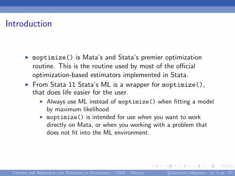
I moptimize() is Mata’s and Stata’s premier optimizationroutine. This is the routine used by most of the officialoptimization-based estimators implemented in Stata.

I From Stata 11 Stata’s ML is a wrapper for moptimize(),that does life easier for the user.

I Always use ML instead of moptimize() when fitting a modelby maximum likelihood

I moptimize() is intended for use when you want to workdirectly on Mata, or when you working with a problem thatdoes not fit into the ML environment.


Mathematical statement of the moptimize() problem

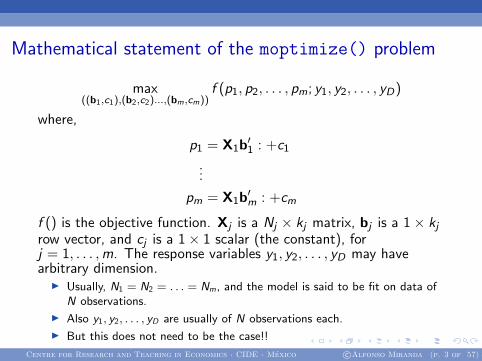
max((b1,c1),(b2,c2)...,(bm,cm))

f (p1, p2, . . . , pm; y1, y2, . . . , yD)

where,

p1 = X1b′1 : +c1

...

pm = X1b′m : +cm

f () is the objective function. Xj is a Nj × kj matrix, bj is a 1× kjrow vector, and cj is a 1× 1 scalar (the constant), forj = 1, . . . ,m. The response variables y1, y2, . . . , yD may havearbitrary dimension.

I Usually, N1 = N2 = . . . = Nm, and the model is said to be fit on data ofN observations.

I Also y1, y2, . . . , yD are usually of N observations each.

I But this does not need to be the case!!


Linear model example

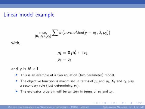
max(b1,c1),(c2)

∑ln(normalden(y − p1, 0, p2))

with,

p1 = X1b′1 : +c1

p2 = c2

and y is N × 1.I This is an example of a two equation (two parameter) model.

I The objective function is maximised in terms of p1 and p2, X1 and c1 playa secondary role (just determining p1).

I The evaluator program will be written in terms of p1 and p2.


Note that the variance s2 is given by p2, and currently, we havep2 = c2, that is, a constant. We could easily write p2 = X2b′2 : +c2and that would allow the variance to depend on a set ofexplanatory variables. From the point of view of moptimize() thismodified problem is the same as the original one.


ML with Moptimize


linear regression with moptimize()

Ok, now to the code. We start defining our mata function, whichwill call linregeval().

sysuse auto, clearmata:function linregeval(transmorphic M, real rowvector b,real colvector lnf){

The first argument defines a handle M (a pointer!!). This handlecontains all the information of our optimisation problem and onceit is set Mata will know what we are talking about everytime weinvoke the handle M. The second argument contains the currentvalue of the coefficients b (which is updated at each iteration step).And the third argument lnf is current log-likelihood value


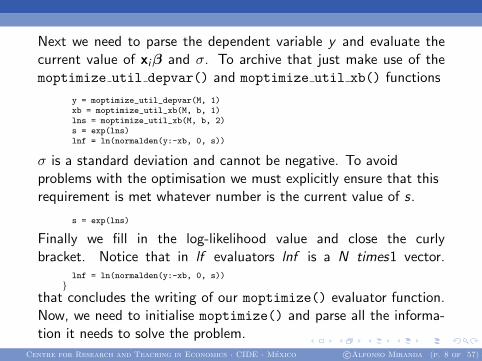
Next we need to parse the dependent variable y and evaluate thecurrent value of xiβ and σ. To archive that just make use of themoptimize util depvar() and moptimize util xb() functions

y = moptimize_util_depvar(M, 1)xb = moptimize_util_xb(M, b, 1)lns = moptimize_util_xb(M, b, 2)s = exp(lns)lnf = ln(normalden(y:-xb, 0, s))

σ is a standard deviation and cannot be negative. To avoidproblems with the optimisation we must explicitly ensure that thisrequirement is met whatever number is the current value of s.

s = exp(lns)

Finally we fill in the log-likelihood value and close the curlybracket. Notice that in lf evaluators lnf is a N times1 vector.

lnf = ln(normalden(y:-xb, 0, s))}

that concludes the writing of our moptimize() evaluator function.Now, we need to initialise moptimize() and parse all the informa-tion it needs to solve the problem.


M = moptimize_init()

moptimize init() initialises moptimize(), allocates memory tothe problem we will work on, and parses that memory address tohandle M. So, moptimize init() creates a pointer but not onlythat.

moptimize_init_evaluator(M, &linregeval())moptimize_init_evaluatortype(M, "lf")

Next, we parse to moptimize() the name of our evaluator. Hereyou’ll see another application of pointers, as we point towardslinregeval() using &linregeval(). Declare the “evaluatortype” using moptimize init evaluatortype(.). In this case wewill use a “lf” evaluator (more of this later).


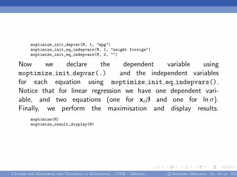
moptimize_init_depvar(M, 1, "mpg")moptimize_init_eq_indepvars(M, 1, "weight foreign")moptimize_init_eq_indepvars(M, 2, "")

Now we declare the dependent variable usingmoptimize init depvar(.) and the independent variablesfor each equation using moptimize init eq indepvars().Notice that for linear regression we have one dependent vari-able, and two equations (one for xiβ and one for lnσ).Finally, we perform the maximisation and display results.

moptimize(M)moptimize_result_display(M)


This is the whole code together

sysuse auto, clearmata:function linregeval(transmorphic M, real rowvector b,real colvector lnf){xb = moptimize_util_xb(M, b, 1)s = moptimize_util_xb(M, b, 2)y = moptimize_util_depvar(M, 1)s = exp(s)lnf = ln(normalden(y:-xb, 0, s))}M = moptimize_init()moptimize_init_evaluator(M, &linregeval())moptimize_init_evaluatortype(M, "lf")

moptimize_init_depvar(M, 1, "mpg")moptimize_init_eq_indepvars(M, 1, "weight foreign")moptimize_init_eq_indepvars(M, 2, "")moptimize(M)moptimize_result_display(M)


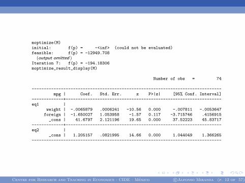
moptimize(M)initial: f(p) = -<inf> (could not be evaluated)feasible: f(p) = -12949.708

(output omitted )Iteration 7: f(p) = -194.18306moptimize_result_display(M)

Number of obs = 74

------------------------------------------------------------------------------mpg | Coef. Std. Err. z P>|z| [95% Conf. Interval]

-------------+----------------------------------------------------------------eq1 |

weight | -.0065879 .0006241 -10.56 0.000 -.007811 -.0053647foreign | -1.650027 1.053958 -1.57 0.117 -3.715746 .4156915

_cons | 41.6797 2.121196 19.65 0.000 37.52223 45.83717-------------+----------------------------------------------------------------eq2 |

_cons | 1.205157 .0821995 14.66 0.000 1.044049 1.366265------------------------------------------------------------------------------


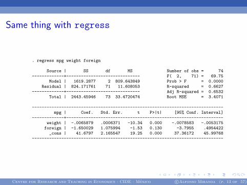
Same thing with regress

. regress mpg weight foreign

Source | SS df MS Number of obs = 74-------------+------------------------------ F( 2, 71) = 69.75

Model | 1619.2877 2 809.643849 Prob > F = 0.0000Residual | 824.171761 71 11.608053 R-squared = 0.6627

-------------+------------------------------ Adj R-squared = 0.6532Total | 2443.45946 73 33.4720474 Root MSE = 3.4071

------------------------------------------------------------------------------mpg | Coef. Std. Err. t P>|t| [95% Conf. Interval]

-------------+----------------------------------------------------------------weight | -.0065879 .0006371 -10.34 0.000 -.0078583 -.0053175

foreign | -1.650029 1.075994 -1.53 0.130 -3.7955 .4954422_cons | 41.6797 2.165547 19.25 0.000 37.36172 45.99768

------------------------------------------------------------------------------


Various flavours

I lf evaluators Requires observation-by-observation calculationof the log-likelihood function (i.e., no good for panel dataestimators because the likelihood is only defined at theindividual/panel level!)

I d evaluators Relaxes the requirement that the log-likelihoodfunction be summable over the observations and thus suitablefor all types of estimators. Robust estimates of variance,adjustment for clustering or survey design is not automaticallydone and dealing with this requires substantial effort


I gf evaluators Relaxes the requirement that the log-likelihoodfunction be summable over the observations and thus suitablefor all types of estimators. Type gf evaluators can work withpanel data models and ‘resurrect’ robust standard errors,clustering, and survey-data adjustments. However, type gf

evaluators are harder to write than lf or d evaluators

I q evaluators are used to deal with quadratic optimisationproblems such as GMM or NLS. These evaluators are suitablefor cross-section and panel data models. The optimiser doesnot return a covariance matrix for the estimated parameters,only point estimates are reported. Estimation of thecovariance matrix should be performed by had using Mata’smatrix algebra facilities.


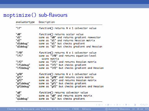
moptimize() sub-flavours


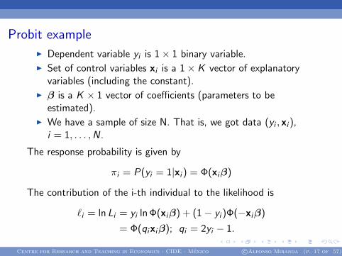
Probit example

I Dependent variable yi is 1× 1 binary variable.

I Set of control variables xi is a 1× K vector of explanatoryvariables (including the constant).

I β is a K × 1 vector of coefficients (parameters to beestimated).

I We have a sample of size N. That is, we got data (yi , xi ),i = 1, . . . ,N.

The response probability is given by

πi = P(yi = 1|xi ) = Φ(xiβ)

The contribution of the i-th individual to the likelihood is

`i = ln Li = yi ln Φ(xiβ) + (1− yi )Φ(−xiβ)

= Φ(qixiβ); qi = 2yi − 1.


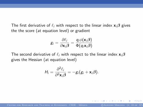
The first derivative of ì with respect to the linear index xiβ givesthe the score (at equation level) or gradient

gi =∂ì∂xiβ

=qiφ(xiβ)

Φ(qixiβ)

The second derivative of ì with respect to the linear index xiβgives the Hessian (at equation level)

Hi =∂2ì∂2xiβ

= −gi (gi + xiβ).


/* Probit by ML d0 with moptimize*/set more offsysuse cancer, cleargen drug2=drug==2gen drug3=drug==3global xvars "drug2 drug3 age"mata:mata clearfunction myprobit_d0(transmorphic M, real scalar todo,real rowvector b, fv, g, H){y = moptimize_util_depvar(M, 1)xb = moptimize_util_xb(M, b, 1)N = rows(y)q = 2*y - J(N,1,1)Sigma = ln(normal(q:*xb))fv = moptimize_util_sum(M, Sigma)}M = moptimize_init()moptimize_init_evaluator(M, &myprobit_d0())moptimize_init_evaluatortype(M, "d0")moptimize_init_depvar(M, 1, "died")moptimize_init_eq_indepvars(M, 1, "drug2 drug3 age")moptimize(M)moptimize_result_display(M)end


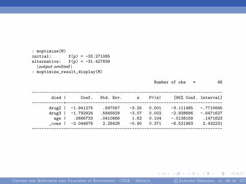
: moptimize(M)initial: f(p) = -33.271065alternative: f(p) = -31.427839

(output omitted ): moptimize_result_display(M)

Number of obs = 48

------------------------------------------------------------------------------died | Coef. Std. Err. z P>|z| [95% Conf. Interval]

-------------+----------------------------------------------------------------drug2 | -1.941275 .597057 -3.25 0.001 -3.111485 -.7710645drug3 | -1.792924 .5845829 -3.07 0.002 -2.938686 -.6471627

age | .0666733 .0410666 1.62 0.104 -.0138158 .1471623_cons | -2.044876 2.28428 -0.90 0.371 -6.521983 2.432231

------------------------------------------------------------------------------


/* probit by ML d1 with moptimize */set more offsysuse cancer, cleargen drug2=drug==2gen drug3=drug==3global xvars "drug2 drug3 age"mata:mata clearfunction myprobit_d1(transmorphic M, real scalar todo,real rowvector b, fv, g, H)

y = moptimize_util_depvar(M, 1)xb = moptimize_util_xb(M, b, 1)N = rows(y)q = 2*y - J(N,1,1)Sigma = ln(normal(q:*xb))fv = moptimize_util_sum(M, Sigma)if (todo>0)d = (q:*normalden(xb)):/normal(q:*xb)g = moptimize_util_vecsum(M, 1, d, fv)

M = moptimize_init()moptimize_init_evaluator(M, &myprobit_d1())moptimize_init_evaluatortype(M, "d1")moptimize_init_depvar(M, 1, "died")moptimize_init_eq_indepvars(M, 1, "drug2 drug3 age")moptimize(M)moptimize_result_display(M)end


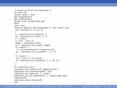
/* Probit by ML d3 with moptimize */set more offsysuse cancer, cleargen drug2=drug==2gen drug3=drug==3global xvars "drug2 drug3 age"mata:mata clearfunction myprobit_d2(transmorphic M, real scalar todo,real rowvector b, fv, g, H){y = moptimize_util_depvar(M, 1)xb = moptimize_util_xb(M, b, 1)N = rows(y)q = 2*y - J(N,1,1)Sigma = ln(normal(q:*xb))fv = moptimize_util_sum(M, Sigma)if (todo>0) {d = (q:*normalden(xb)):/normal(q:*xb)g = moptimize_util_vecsum(M, 1, d, fv)}if (todo>1) {Dd = J(N,1,-1):*d:*(d+xb)H = moptimize_util_matsum(M, 1, 1, Dd, fv)}}M = moptimize_init()moptimize_init_evaluator(M, &myprobit_d2())moptimize_init_evaluatortype(M, "d2")moptimize_init_depvar(M, 1, "died")moptimize_init_eq_indepvars(M, 1, "drug2 drug3 age")moptimize(M)moptimize_result_display(M)end


/* probit by ML gf1 with moptimize */set more offuse http://www.stata-press.com/data/r12/unionglobal xvars "age grade not_smsa year south"mata:mata clearfunction myprobit_gf1(transmorphic M, real scalar todo,real rowvector b, fv, g, H){y = moptimize_util_depvar(M, 1)xb = moptimize_util_xb(M, b, 1)N = rows(y)q = 2*y - J(N,1,1)fv = ln(normal(q:*xb))if (todo>0) {st_view(X,.,tokens(st_global("xvars")))one = J(rows(X),1,1)X = (X,one)g = (q:*normalden(xb)):/normal(q:*xb)g = g:*X}}M = moptimize_init()moptimize_init_evaluator(M, &myprobit_gf1())moptimize_init_evaluatortype(M, "gf1")moptimize_init_vcetype(M, "robust")moptimize_init_cluster(M, "idcode")moptimize_init_depvar(M, 1, "union")moptimize_init_eq_indepvars(M, 1, "$xvars")moptimize(M)moptimize_result_display(M)end


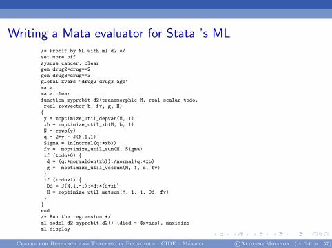
Writing a Mata evaluator for Stata ’s ML/* Probit by ML with ml d2 */set more offsysuse cancer, cleargen drug2=drug==2gen drug3=drug==3global xvars "drug2 drug3 age"mata:mata clearfunction myprobit_d2(transmorphic M, real scalar todo,real rowvector b, fv, g, H){y = moptimize_util_depvar(M, 1)xb = moptimize_util_xb(M, b, 1)N = rows(y)q = 2*y - J(N,1,1)Sigma = ln(normal(q:*xb))fv = moptimize_util_sum(M, Sigma)if (todo>0) {d = (q:*normalden(xb)):/normal(q:*xb)g = moptimize_util_vecsum(M, 1, d, fv)}if (todo>1) {Dd = J(N,1,-1):*d:*(d+xb)H = moptimize_util_matsum(M, 1, 1, Dd, fv)}}end/* Run the regression */ml model d2 myprobit_d2() (died = $xvars), maximizeml display


GMM with Moptimize


Introduction

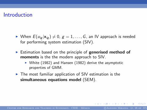
I When E (uig |xig ) 6= 0, g = 1, . . . ,G , an IV approach is neededfor performing system estimation (SIV).

I Estimation based on the principle of generised method ofmoments is the the modern approach to SIV.

I White (1982) and Hansen (1982) derive the asymptoticproperties of GMM.

I The most familiar application of SIV estimation is thesimultaneous equations model (SEM).


Example

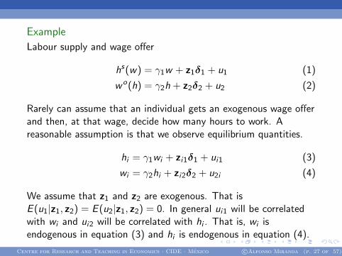
Labour supply and wage offer

hs(w) = γ1w + z1δ1 + u1 (1)

wo(h) = γ2h + z2δ2 + u2 (2)

Rarely can assume that an individual gets an exogenous wage offerand then, at that wage, decide how many hours to work. Areasonable assumption is that we observe equilibrium quantities.

hi = γ1wi + zi1δ1 + ui1 (3)

wi = γ2hi + zi2δ2 + u2i (4)

We assume that z1 and z2 are exogenous. That isE (u1|z1, z2) = E (u2|z1, z2) = 0. In general ui1 will be correlatedwith wi and ui2 will be correlated with hi . That is, wi isendogenous in equation (3) and hi is endogenous in equation (4).


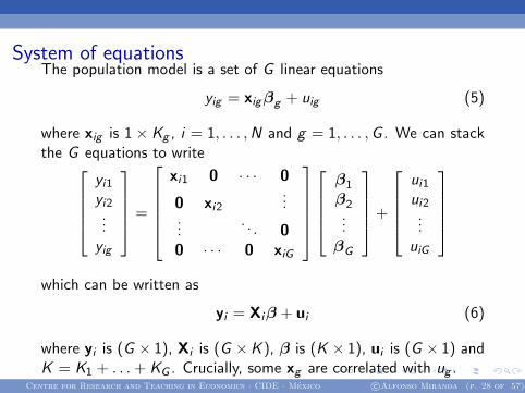
System of equationsThe population model is a set of G linear equations

yig = xigβg + uig (5)

where xig is 1× Kg , i = 1, . . . ,N and g = 1, . . . ,G . We can stackthe G equations to write

yi1yi2...yig

=

xi1 0 · · · 0

0 xi2...

.... . . 0

0 · · · 0 xiG

β1

β2...

βG

+

ui1ui2...

uiG

which can be written as

yi = Xiβ + ui (6)

where yi is (G × 1), Xi is (G ×K ), β is (K × 1), ui is (G × 1) andK = K1 + . . .+ KG . Crucially, some xg are correlated with ug .


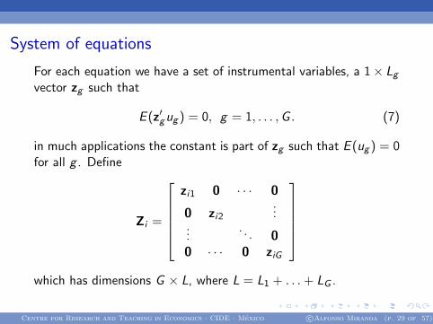
System of equations

For each equation we have a set of instrumental variables, a 1× Lgvector zg such that

E (z′gug ) = 0, g = 1, . . . ,G . (7)

in much applications the constant is part of zg such that E (ug ) = 0for all g . Define

Zi =

zi1 0 · · · 0

0 zi2...

.... . . 0

0 · · · 0 ziG

which has dimensions G × L, where L = L1 + . . .+ LG .


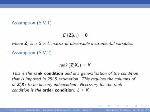
Assumption (SIV.1)

E(Z′iui

)= 0

where Zi is a G × L matrix of observable instrumental variables.

Assumption (SIV.2)

rank(Z′iXi

)= K

This is the rank condition and is a generalisation of the conditionthat is imposed in 2SLS estimation. This requires the columns ofof Z′iXi to be linearly independent. Necessary for the rankcondition is the order condition: L ≥ K .


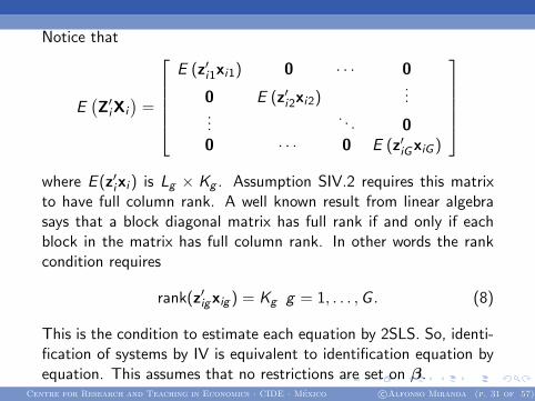
Notice that

E(Z′iXi

)=

E (z′i1xi1) 0 · · · 0

0 E (z′i2xi2)...

.... . . 0

0 · · · 0 E (z′iGxiG )

where E (z′ixi ) is Lg × Kg . Assumption SIV.2 requires this matrixto have full column rank. A well known result from linear algebrasays that a block diagonal matrix has full rank if and only if eachblock in the matrix has full column rank. In other words the rankcondition requires

rank(z′igxig ) = Kg g = 1, . . . ,G . (8)

This is the condition to estimate each equation by 2SLS. So, identi-fication of systems by IV is equivalent to identification equation byequation. This assumes that no restrictions are set on β.


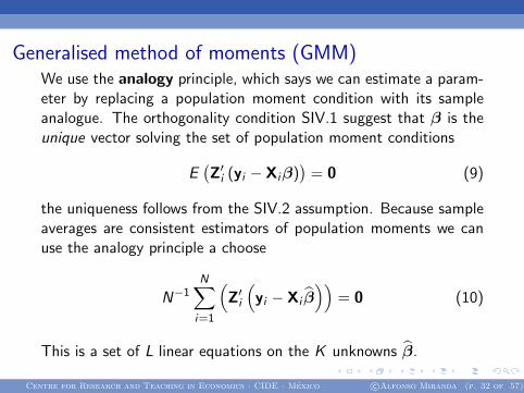
Generalised method of moments (GMM)We use the analogy principle, which says we can estimate a param-eter by replacing a population moment condition with its sampleanalogue. The orthogonality condition SIV.1 suggest that β is theunique vector solving the set of population moment conditions

E(Z′i (yi − Xiβ)

)= 0 (9)

the uniqueness follows from the SIV.2 assumption. Because sampleaverages are consistent estimators of population moments we canuse the analogy principle a choose

N−1N∑i=1

(Z′i

(yi − Xi β

))= 0 (10)

This is a set of L linear equations on the K unknowns β.


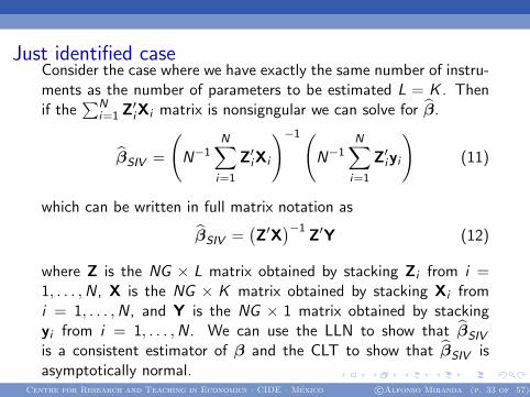
Just identified caseConsider the case where we have exactly the same number of instru-ments as the number of parameters to be estimated L = K . Thenif the

∑Ni=1 Z

′iXi matrix is nonsigngular we can solve for β.

βSIV =

(N−1

N∑i=1

Z′iXi

)−1(N−1

N∑i=1

Z′iyi

)(11)

which can be written in full matrix notation as

βSIV =(Z′X

)−1Z′Y (12)

where Z is the NG × L matrix obtained by stacking Zi from i =1, . . . ,N, X is the NG × K matrix obtained by stacking Xi fromi = 1, . . . ,N, and Y is the NG × 1 matrix obtained by stackingyi from i = 1, . . . ,N. We can use the LLN to show that βSIV

is a consistent estimator of β and the CLT to show that βSIV isasymptotically normal.


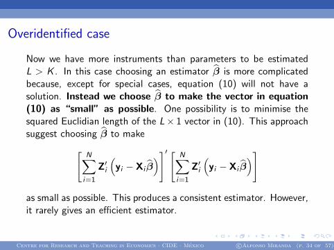
Overidentified case

Now we have more instruments than parameters to be estimatedL > K . In this case choosing an estimator β is more complicatedbecause, except for special cases, equation (10) will not have asolution. Instead we choose β to make the vector in equation(10) as “small” as possible. One possibility is to minimise thesquared Euclidian length of the L× 1 vector in (10). This approachsuggest choosing β to make[

N∑i=1

Z′i

(yi − Xi β

)]′ [ N∑i=1

Z′i

(yi − Xi β

)]

as small as possible. This produces a consistent estimator. However,it rarely gives an efficient estimator.


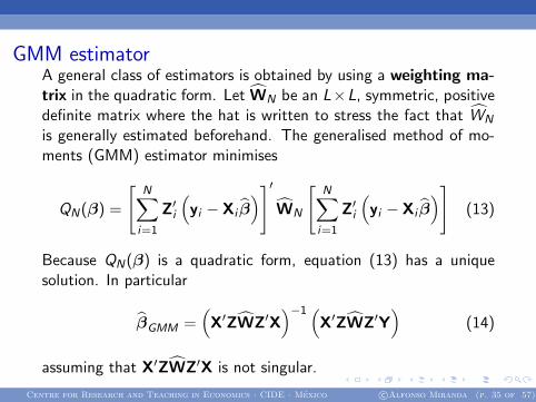
GMM estimatorA general class of estimators is obtained by using a weighting ma-trix in the quadratic form. Let WN be an L×L, symmetric, positivedefinite matrix where the hat is written to stress the fact that WN

is generally estimated beforehand. The generalised method of mo-ments (GMM) estimator minimises

QN(β) =

[N∑i=1

Z′i

(yi − Xi β

)]′WN

[N∑i=1

Z′i

(yi − Xi β

)](13)

Because QN(β) is a quadratic form, equation (13) has a uniquesolution. In particular

βGMM =(X′ZWZ′X

)−1 (X′ZWZ′Y

)(14)

assuming that X′ZWZ′X is not singular.


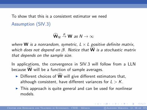
To show that this is a consistent estimator we need

Assumption (SIV.3)

WNp→W as N →∞

where W is a nonrandom, symetric, L× L positive definite matrix,which does not depend on β. Notice that W is a stochastic matrixthat depends on the sample size.

In applications, the convergence in SIV.3 will follow from a LLNbecause W will be a function of sample averages.

I Different choices of W will give different estimators that,although consistent, have different variances for L > K .

I This approach is quite general and can be used for nonlinearmodels.


Is easy to show that the GMM estimator βGMM is

I A consistent estimator for β.

I Asymptotically normal.


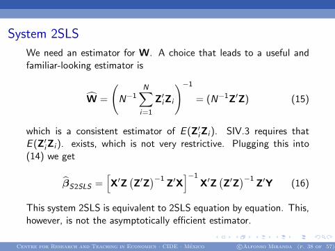
System 2SLS

We need an estimator for W. A choice that leads to a useful andfamiliar-looking estimator is

W =

(N−1

N∑i=1

Z′iZi

)−1= (N−1Z′Z) (15)

which is a consistent estimator of E (Z′iZi ). SIV.3 requires thatE (Z′iZi ). exists, which is not very restrictive. Plugging this into(14) we get

βS2SLS =[X′Z

(Z′Z

)−1Z′X

]−1X′Z

(Z′Z

)−1Z′Y (16)

This system 2SLS is equivalent to 2SLS equation by equation. This,however, is not the asymptotically efficient estimator.


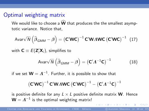
Optimal weighting matrix

We would like to choose a W that produces the the smallest asymp-totic variance. Notice that,

Avar√N(βGMM − β

)=(C′WC

)−1C′WΛWC

(C′WC

)−1(17)

with C ≡ E (Z′iXi ), simplifies to

Avar√N(βGMM − β

)=(C′Λ−1C

)−1(18)

if we set W = Λ−1. Further, it is possible to show that(C′WC

)−1C′WΛWC

(C′WC

)−1 − (C′Λ−1C)−1is positive definite for any L× L positive definite matrix W. HenceW = Λ−1 is the optimal weighting matrix!


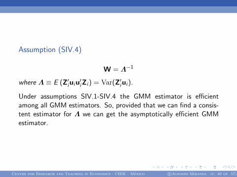
Assumption (SIV.4)

W = Λ−1

where Λ ≡ E (Z′iuiu′iZi ) = Var(Z′iui ).

Under assumptions SIV.1-SIV.4 the GMM estimator is efficientamong all GMM estimators. So, provided that we can find a consis-tent estimator for Λ we can get the asymptotically efficient GMMestimator.


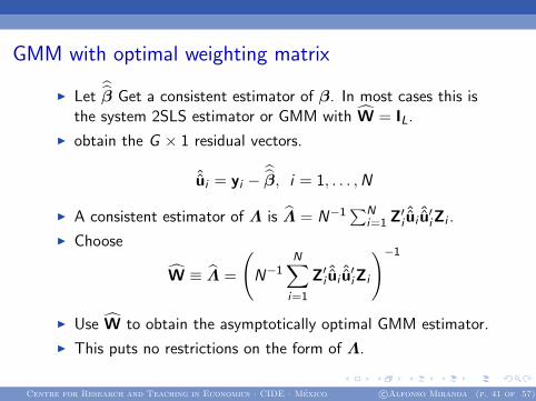
GMM with optimal weighting matrix

I Letβ Get a consistent estimator of β. In most cases this is

the system 2SLS estimator or GMM with W = IL.

I obtain the G × 1 residual vectors.

ûi = yi −β, i = 1, . . . ,N

I A consistent estimator of Λ is Λ = N−1∑N

i=1 Z′iûi û′iZi .

I Choose

W ≡ Λ =

(N−1

N∑i=1

Z′i ûi û′iZi

)−1I Use W to obtain the asymptotically optimal GMM estimator.

I This puts no restrictions on the form of Λ.


The assynptotic variance of the optimal GMM estimator is

Avar(βGMM

)=

(X′Z)( N∑i=1

Z′i ui u′iZ

)−1 (Z′X

)−1

where ui = yi − Xi βGMM . Asymptotically it makes no differenceif the first-stage residuals ˆui are used. This is called the minimumchi-square estimator.


Remarks

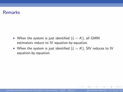
I When the system is just identified (L = K ), all GMMestimators reduce to IV equation-by-equation.

I When the system is just identified (L = K ), SIV reduces to IVequation-by-equation.


Hypothesis testing

Under SIV.1-SIV.4 we can proceed as usual

I Confidence intervals.

I t statistics and test are valid (and robust toheteroskedasticity).

I Wald tests and F -tests.


Testing overidentification restrictions

When L > K we can test whether overidentifying restrictions arevalid. It can be shown that(

N−1/2N∑i=1

Z′i ui

)′W

(N−1/2

N∑i=1

Z′i ui

)a∼ χ2

(L−K) (19)

under the null H0: E (Z′iui ) = 0. Because we have used K orthogo-

nality conditions to estimate βGMM we loss K degrees of freedom.

Notice that here we use the optimal weighting matrix W , other-wise the statistics does not have a limiting chi-square distribution.When L = K the left hand side is exactly zero and there are nooveridentifying restrictions to be tested.


Testing overidentification restrictions

Other (equivalent) names for the over identification test are

I Hansen’s test

I Sargan’s test

I Hansen-Sargan test.


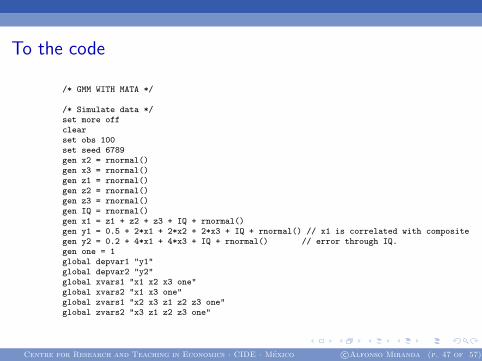
To the code

/* GMM WITH MATA */

/* Simulate data */set more offclearset obs 100set seed 6789gen x2 = rnormal()gen x3 = rnormal()gen z1 = rnormal()gen z2 = rnormal()gen z3 = rnormal()gen IQ = rnormal()gen x1 = z1 + z2 + z3 + IQ + rnormal()gen y1 = 0.5 + 2*x1 + 2*x2 + 2*x3 + IQ + rnormal() // x1 is correlated with compositegen y2 = 0.2 + 4*x1 + 4*x3 + IQ + rnormal() // error through IQ.gen one = 1global depvar1 "y1"global depvar2 "y2"global xvars1 "x1 x2 x3 one"global xvars2 "x1 x3 one"global zvars1 "x2 x3 z1 z2 z3 one"global zvars2 "x3 z1 z2 z3 one"


/* Bring Data to Mata */matamata cleary1 = NULLy2 = NULLX1 = NULLX2 = NULLZ1 = NULLZ2 = NULLst_view(y1,.,"$depvar1")st_view(y2,.,"$depvar2")st_view(X1,.,"$xvars1")st_view(X2,.,"$xvars2")st_view(Z1,.,"$zvars1")st_view(Z2,.,"$zvars2")/* obtain number of individuals */N = rows(y1)/* Define y */for (i=1;i<=N;i++) {if (i==1) y=(y1[i]\y2[i])else y = (y\(y1[i]\y2[i]))}


/* Define X */for (i=1;i<=N;i++) {if (i==1) X=blockdiag(X1[i,],X2[i,])else {X = (X\blockdiag(X1[i,],X2[i,]))}}/* Define Z */for (i=1;i<=N;i++) {if (i==1) Z=blockdiag(Z1[i,],Z2[i,])else {Z = (Z\blockdiag(Z1[i,],Z2[i,]))}}/* Start with an identity matrix weighting matrix */Wopt = I(cols(Z))/* perform GMM optimisation */***Define evaluator functionfunction oiv_gmm0(transmorphic M, real scalar todo,real rowvector b, q,S) {y1 = moptimize_util_depvar(M,1)y2 = moptimize_util_depvar(M,2)xb1 = moptimize_util_xb(M,b,1)xb2 = moptimize_util_xb(M,b,2)st_view(Z1,.,moptimize_util_userinfo(M, 2))st_view(Z2,.,moptimize_util_userinfo(M, 4))N = rows(y1)


/* Define y */for (i=1;i<=N;i++) {if (i==1) y=(y1[i]\y2[i])else y = (y\(y1[i]\y2[i]))}

/* Define Z */for (i=1;i<=N;i++) {if (i==1) Z=blockdiag(Z1[i,],Z2[i,])else {Z = (Z\blockdiag(Z1[i,],Z2[i,]))}}e = y - xbq = Z’*e}** initialise moptimizeM = moptimize_init()moptimize_init_evaluator(M, & oiv_gmm0())moptimize_init_evaluatortype(M, "q0")moptimize_init_ndepvars(M, 2)moptimize_init_depvar(M, 1, "y1")moptimize_init_depvar(M, 2, "y2")moptimize_init_eq_indepvars(M, 1, "x1 x2 x3")moptimize_init_eq_indepvars(M, 2, "x1 x3")moptimize_init_userinfo(M, 1, ("x1", "x2", "x3","one"))moptimize_init_userinfo(M, 2, ("x2", "x3","z1","z2","z3","one"))moptimize_init_userinfo(M, 3, ("x1", "x3","one"))moptimize_init_userinfo(M, 4, ("x3","z1","z2","z3","one"))moptimize_init_gnweightmatrix(M,Wopt)moptimize_init_which(M, "min")


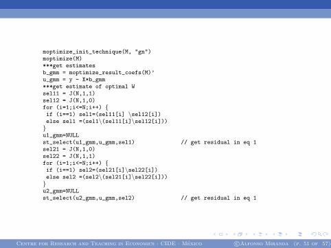
moptimize_init_technique(M, "gn")moptimize(M)***get estimatesb_gmm = moptimize_result_coefs(M)’u_gmm = y - X*b_gmm***get estimate of optimal Wsel11 = J(N,1,1)sel12 = J(N,1,0)for (i=1;i<=N;i++) {if (i==1) sel1=(sel11[i] \sel12[i])else sel1 =(sel1\(sel11[i]\sel12[i]))}u1_gmm=NULLst_select(u1_gmm,u_gmm,sel1) // get residual in eq 1sel21 = J(N,1,0)sel22 = J(N,1,1)for (i=1;i<=N;i++) {if (i==1) sel2=(sel21[i]\sel22[i])else sel2 =(sel2\(sel21[i]\sel22[i]))}u2_gmm=NULLst_select(u2_gmm,u_gmm,sel2) // get residual in eq 1


for (i=1;i<=N;i++) { // get N^(-1) Sum(Zi’uiui’Zi)if (i==1) {Zi = blockdiag(Z1[i,],Z2[i,])ui = u1_gmm[i]\u2_gmm[i]D = Zi’*ui*ui’*Zi}else {Zi = blockdiag(Z1[i,],Z2[i,])ui = u1_gmm[i]\u2_gmm[i]D = D + Zi’*ui*ui’*Zi}}D = (1/N)*DWopt = invsym(D)*** re-optimizeM = moptimize_init()moptimize_init_evaluator(M, & oiv_gmm0())moptimize_init_evaluatortype(M, "q0")moptimize_init_ndepvars(M, 2)moptimize_init_depvar(M, 1, "y1")moptimize_init_depvar(M, 2, "y2")moptimize_init_eq_indepvars(M, 1, "x1 x2 x3")moptimize_init_eq_indepvars(M, 2, "x1 x3")moptimize_init_userinfo(M, 1, ("x1", "x2", "x3","one"))moptimize_init_userinfo(M, 2, ("x2", "x3","z1","z2","z3","one"))moptimize_init_userinfo(M, 3, ("x1", "x3","one"))moptimize_init_userinfo(M, 4, ("x3","z1","z2","z3","one"))moptimize_init_gnweightmatrix(M,Wopt)moptimize_init_which(M, "min")


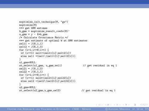
moptimize_init_technique(M, "gn")moptimize(M)*** get GMM estimesb_gmm = moptimize_result_coefs(M)’u_gmm = y - X*b_gmm/* Calculate Covariance Matrix */*** get estimate of optimal W at GMM estimatessel11 = J(N,1,1)sel12 = J(N,1,0)for (i=1;i<=N;i++) {if (i==1) sel1=(sel11[i]\sel12[i])else sel1 =(sel1\(sel11[i]\sel12[i]))}u1_gmm=NULLst_select(u1_gmm, u_gmm,sel1) // get residual in eq 1sel21 = J(N,1,0)sel22 = J(N,1,1)for (i=1;i<=N;i++) {if (i==1) sel2=(sel21[i]\sel22[i])else sel2 =(sel2\(sel21[i]\sel22[i]))}u2_gmm=NULLst_select(u2_gmm,u_gmm,sel2) // get residual in eq 1


for (i=1;i<=N;i++) { // get N^(-1) Sum(Zi’uiui’Zi)if (i==1) {Zi = blockdiag(Z1[i,],Z2[i,])ui = u1_gmm[i]\u2_gmm[i]D = Zi’*ui*ui’*Zi}else {Zi = blockdiag(Z1[i,],Z2[i,])ui = u1_gmm[i]\u2_gmm[i]D = D + Zi’*ui*ui’*Zi}}Wopt = invsym(D)/* Calculate covariance matrix */V_gmm = invsym((X’*Z)*Wopt*Z’X)/* parse results to stata */moptimize_result_post(M, "robust")st_matrix("b_gmm", b_gmm’)st_matrix("V_gmm", V_gmm)end/* post estimates to stata */program drop _allprogram mypost, eclassereturn repost b=b_gmm V=V_gmmendmypost


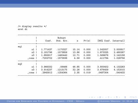
/* display results */eret di

------------------------------------------------------------------------------| Robust| Coef. Std. Err. z P>|z| [95% Conf. Interval]

-------------+----------------------------------------------------------------eq1 |

x1 | 1.771437 .1170327 15.14 0.000 1.542057 2.000817x2 | 2.181796 .1573859 13.86 0.000 1.873325 2.490267x3 | 1.855917 .1460442 12.71 0.000 1.569676 2.142158

_cons | .7202702 .1573938 4.58 0.000 .411784 1.028756-------------+----------------------------------------------------------------eq2 |

x1 | 3.966332 .08466 46.85 0.000 3.800402 4.132263x3 | 3.914237 .1213175 32.26 0.000 3.676459 4.152015

_cons | .2945812 .1254364 2.35 0.019 .0487304 .540432------------------------------------------------------------------------------


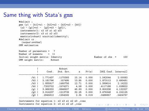
Same thing with Stata’s gmm#delimit ;gmm (y1 - {b1}*x1 - {b2}*x2 - {b3}*x3 - {b0})(y2 - {g1}*x1 - {g2}*x3 - {g0}),instruments(1: x2 x3 z1 z2 z3)instruments(2: x3 z1 z2 z3)wmatrix(robust) winitial(identity);

#delimit cr(output omitted )

GMM estimation

Number of parameters = 7Number of moments = 11Initial weight matrix: Identity Number of obs = 100GMM weight matrix: Robust

------------------------------------------------------------------------------| Robust| Coef. Std. Err. z P>|z| [95% Conf. Interval]

-------------+----------------------------------------------------------------/b1 | 1.771437 .1170393 15.14 0.000 1.542044 2.00083/b2 | 2.181796 .157495 13.85 0.000 1.873112 2.490481/b3 | 1.855917 .1460756 12.71 0.000 1.569614 2.14222/b0 | .7202702 .1574271 4.58 0.000 .4117188 1.028822/g1 | 3.966332 .0846927 46.83 0.000 3.800338 4.132327/g2 | 3.914237 .1213739 32.25 0.000 3.676348 4.152125/g0 | .2945812 .1254592 2.35 0.019 .0486857 .5404767

------------------------------------------------------------------------------Instruments for equation 1: x2 x3 z1 z2 z3 _consInstruments for equation 2: x3 z1 z2 z3 _cons


References

I Cameron, C.A.; Trivedi, P.K. (2005). Microeconometrics: Methods andApplications. Cambridge University Press.

I Cameron, C.A.; Trivedi, P.K (2010). Microeconometrics Using Stata, RevisedEdition. Stata Press.

I Hansen, LP. (1982). Large sample properties of generalised method of momentsestimators. Econometrica 50: 1029-1054.

I White, H. (1982). Instrumental variable estimation with independentobservations. Econometrica 50: 483-499.

I Wooldridge, J.M. (2010). Econometric Analysis of Cross Section and PanelData (2nd edition). The MIT Press.


gmm and maximum likelihood estimators with mata and … · finally we ll in the log-likelihood...

Documents