NBER WORKING PAPER SERIES

GOOD POLICY OR GOOD LUCK?COUNTRY GROWI'H PERFORMANCE

AND TEMPORARY SHOCKS

William EasterlyMichael KremerLain Pritchett

Lawrence H. Summers

Working Paper No. 4474

NATIONAL BUREAU OF ECONOMIC RESEARCH1050 Massachusetts Avenue

Cambridge, MA 02138September 1993

We are grateful to an anonymous referee, Robert Barro, Nancy Birdsall, Olivier Blanchard,Michael Bruno, Daniel Cohen, Brad Dc Long, Stanley Fischer, Chad Jones, Robert King, RossLevine, Johannes Linn, Ramon Marimon, Robert Murphy, Sergio Rebelo, Fabio Schiantarelli,Paul Romer, and Nick Stern for comments and useful discussions, to participants in the growthconference in Estoril, Portugal in January 1993 (especially our discussant Danny Quah) and inthe growth conference in the World Bank February 1993 (again especially our discussant AlanStockman), and to George Clarke and Sheryl Sandberg for research assistance. Any remainingerrors are the responsibility of the authors. This paper is part of NBER's research program inGrowth. Any opinions expressed are those of the authors and not those of the Department of theTreasury, the World Bank, or the National Bureau of Economic Research.

NBER Working Paper #4474September 1993

GOOD POLICY OR GOOD LUCK?COUNTRY GROWTH PERFORMANCE

AND TEMPORARY SHOCKS

ABSTRACT

Much of the new growth literature stresses countly characteristics, such as education levels or

political stability, as the dominant determinant of growth. However, growth rates are highly

unstable over time, with a correlation across decades of .1 to .3, while country characteristics are

stable, with cross-decade correlations of .6 to .9. Shocks, especially those to terms of trade, play

a large role in explaining variance in growth. These findings suggest either that shocks are

important relative to country characteristics in determining long-run growth, or that worldwide

technological change determines long-run growth while country characteristics determine relative

income levels.

William EasterlyThe World Bank1818 H Street, NWWashington, D.C. 20433

Lant PritchettThe World Bank1818 H Street, NWWashington, D.C. 20433

Michael KremerDepartment of Economics E52-262BMassachusetts Institute of

TechnologyCambridge, MA 02139and NBER

Lawrence H. SummersUnder Secretary for International AffairsDepartment of the Treasury, Room 34321500 Pennsylvania Avenue, NWWashington, D.C. 20220and NBER

2

Introduction

Much of the new growth literature stresses country characteristics as the dominant determinant

of growth performance. A vast empirical literature tests the effects of country characteristics on

growth.' This paper presents a fact suggesting the emphasis on country characteristics is misguided:

growth rates are highly unstable over time, while country characteristics are highly persistent. The

correlation across decades of countries' growth rates of income per capita is around .1(0 .3. while

most country characteristics display cross-decade correlations of .6 to .9. Correlations of growth

across periods as long as two decades — period lengths comparable to those used in the cross-section

empirical literature — are similarly low. With a few famous exceptions, the same countries do not do

well period after period; countries are 'success stories' one period and disappointments the next.

The low persistence of growth rates reconciles the enormous variation in growth rates across

countries with the remarkable stability of relative incomes across countries. For each of the last two

decades the standard deviation of growth rates has been over 2.5, nearly the growth difference

between Japan and the US. Yet the correlation of (Summers and Heston (1991)) GDP per capita in

1960 and 1988 was .92. Even more striking the rank correlation of GDP per capita for the 28

countries for which Maddison (1989) has data is .82 over 1870-1988. Major changes in country

income ranldngs would have required large persistent differences in growth rwts; in the event,

income rankings did not change much and only a small fraction of the growth differences between

countries were persistent.

Among the counny ch cicflsdca this Ilicrasot cuisines ale policies affecisag the price or quanety of equipnient Invesuneit (Do Longand Summers (1991. 1992, 1993), polEles aflcciing rnseaith and dentopmenn(Romef (1989.1990)), inveignenl in physical capial(Romer (1986. 1991)) huisin capinll (Lucai (1988). Bum (1991). Bonn and Lee (1993)). mmii inco (Basis (1991)). distorsonary

policy esvtrvnmems (Murpfly. Shleifer. sod vishny (l991). Easierly (1993)). government spending (Basis (1990). isa policy (King auRebolo (1990). Jones vii Manaelli(1990)). rii policy (King and Levine (1993). Levine (1991). Oseenwood and Jovanovic (1990).

0db ((989)). trade policy (Youii (1991). Grossman and Helpinin (1991). Riveit Bonn sod Romer (1991). Horniest (1991)). alconsid,smbuaon (Alesins and Rodrik (199)), Perasoca and Tabellini (1991)), macroeconomic policy (Fischer (1991. 1993)) and even ediiucuy

(Bor)as ((992)), legal inseiwdoni (North (1989)) and teligioa (Dc Long (1988)).

3

This paper has three sections and a conclusion. The first section presents the basic facts about

persistence of cross country growth differences and of country characteristics. The second section

attempts to identify the temporary shocks important in explaining low persistence of growth rates

across decades. The third section interprets low persistence under two types of growth models:

models in which country characteristics determine long-run growth rates and models in which country

characteristics determine relative levels of steady state income and long-run growth rates are

determined by worldwide technological change. A conclusion summarizes the results.

I) Low Persistence of Growth Rate DilTerences Across Countries

(a) Bcic facts

The persistence of growth rate differences across countries, even over long periods, is low.

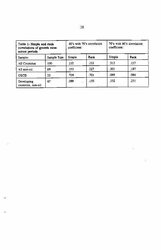
Table 1 presents correlations of the least-squares growth rate of GDP per worker between 1960-69,

1970-79 and 1980-88. The R2 obtained by regressing the current growth rate on the previous

decade's growth was less than 10 percent. Little of the variation of growth rates is explained by past

growth.3 This low persistence result is robust over the choice of country sample, time period, and

sectors] performance measure.

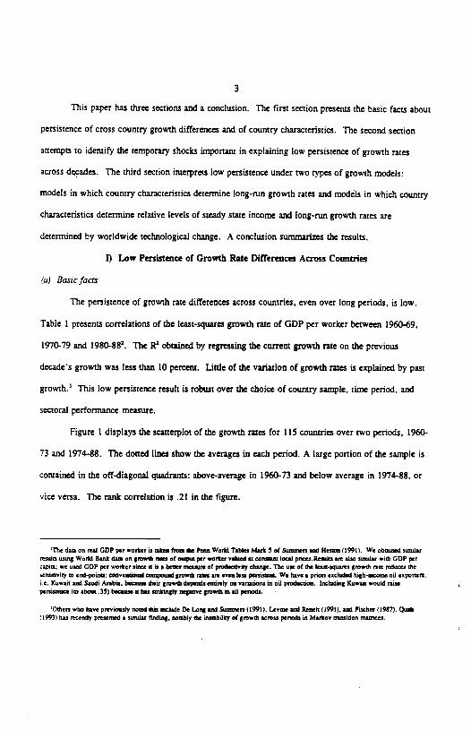
Figure 1 displays the scatterplot of the growth razes for 115 countries over two periods, 1960-.

73 and 1974-88. The dotted lines show the averages in each period. A large portion of the sample is

contained in the off-diagonal quadrants: above-average in 1960-73 and below average in 1974-88, or

vice versa. The rank correlation is 21 in the figure.

'The dam on real GOP per worker is iakesi from the Penn World TablesMark 5 of Summers and Hesmon (1991). We obiau similarrenilo using World Bank dam on growth rows of owpee perworkervalued ii comomea local pnces.RumdO iso alto similar with GOP percapiw: we used GOP per worker sara is is a bewse aure of preducuvity change. The use of the lease-squares growth rue reduces thesonsmoviry in end-poino: conventional cosirpowal growth iown iso even less peroisinsa. We have a prrofl occluded high-income od exporTers.i.e. Kuwait aid Saudi Arabia. because their growth depends enorely on varwsona in oil production. Including Kuwaie would raiseperaisreere (To about .35) because it has irkingly aeganve growth in all periods.

'Others who have previously nosed dim iodide De Long and Suounero (1991). Levine and Rutsok (1991). and Fitcher (1987). Qush(I 993) hat recendy proseneeda sunilar finding, nombly the insiabiliry of growth across penoda in Markov Transition maresces.

4

The boxes in the corners represent the deciles of the period growth rates. The northeast box

represents countries with growth in the top deciles in both periods. The southwest box shows the

countries persistently in the bottom decile. The northeast box (persistent success) contains Botswana

and the famous Asian Gang of Four (Hong Kong is actually just short of being in the top decile in the

tirst period). The East Asian success story is well Imown, while Botswana has benefitted from

extensive diamond mines and from a democratic government that has avoided some of its neighbors'

economic mistakes. The widespread perception of strong country effects in growth is strongly

influenced by the Gang of Four; without them and Botswana, the already low correlation of growth

rates between periods is cut in half. In contrast, persistence is not raised much by deleting a small

number of outliers.

Persistence is also low for several subsamples of countries. The second, third and fourth rows

of Table 1 show the correlations for non-oil countries, the OECD countries, and the non-oil

developing countries. The only exception is a high correlation between the 60's and 70's in the small

sample of OECD countries, but this reverts to zero between the 70's and 80's.

Figure 2 shows that persistence stays low at various period lengths in the postwar data. This

is confirmed by partial data on long-run growth rates for 30 year periods over 1870-1988'. We have

a total of 54 observations for 23 OECD and Latin American countries. Figure 3 shows growth plotted

against lagged growth for these 30 year periods. Portugal is illustrative: decent growth in 1870-99,

negative growth in 1900-29, average growth in 1930-59. and one of the highest growth rates in 1960-

'We have calculaced the Iesat..quaii growth rum of per capim incoren dam borrowed from EesrrIy ted RebelO (1993). who use muurJyMaddison (1959). it need baldly be mid this tha dam u even more subjec* is error than the recent dam. untiuding error! asaoduced by

esreapolenon over long persodu.

5

88. The correlation of 30-year per capita growth with per capita growth in the previous 30 year

period in this data is only .l2.

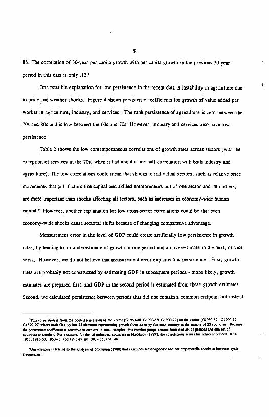
One possible explanation for low persistence in the recent data is instability in agriculture due

to price and weather shocks. Figure 4 shows persistence coefficients for growth of value added per

worker in agriculture, industry, and services. The rank persistence of agriculture is zero between the

70s and 80s and is low between the 60s and 70s. However, industry and services also have low

persistence.

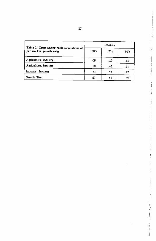
Table 2 shows the low contemporaneous correlations of growth rates across sectors (with the

exception of services in the 70s, when it had about a one-half correlation with both industry and

agriculture). The low correlations could mean that shocks to individual sectors, such as relative price

movements that pull factors like capital and skilled entrepreneurs out of one sector and into others,

are more important than shocks affecting all sectors, such as increases in economy-wide human

capital.6 However, another explanation for low cross-sector correlations could be that even

economy-wide shocks cause sectoral shifts because of changing comparative advantage.

Measurement error in the level of GDP could create artificially low persistence in growth

rates, by leading to an underestimate of growth in one period and an overestimate in the next, or vice

versa. However, we do not believe that measurement error explains low persistence. First, growth

rates are probably not constructed by estimating GDP in subsequent periods - more likely, growth

estimates are prepared first, and GDP in the second period is estimated from these growth estimates.

Second, we calculated persistence between periods that did not contain a common endpoint but instead

'Thio conoIoon u from the pooled regremon of the vecmr 101960-aS 01930-59 GI9)-291 on the vector (01930-59 G19-2901870-991 whore each Oox-yy baa 23 elements represenong growth from xx toyy for each coustoy in the simple of 23 cOufloles. Becausethe penasleisee coefficient is neosidve to outhers in snsiul samples, this msmberjumps around from em set of periods oral one set ofcountries to another. For eumple. for the 16 industhalcouneses in Maddison (1989). the correlanons ictors his a4jacrnt penodi 870-1913. 1913-50. 1950-73. and 1973-81 ate .38. -.35. anti .46.

Oar ozercixe is related so the analysis of Stocbsian (1988) this examines sector-specific oral counny-opecific ihocks at business-cycle

frequeociei.

6

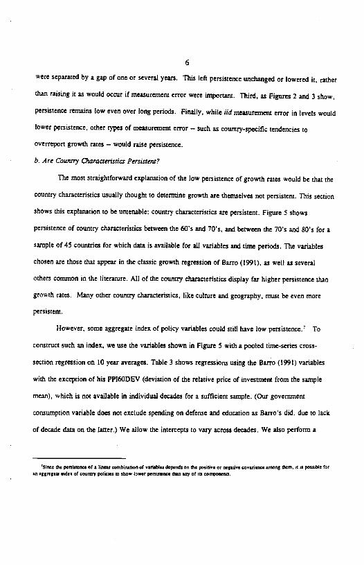
were separated by a gap of one or several years. This left persistence unchanged or lowered it. rather

than raising it as would occur if measurement error were important. Third. as Figures 2 and 3 show.

persistence remains tow even over tong periods. Finally, while iid measurement error in levels would

tower persistence, other types of measurement error — such as country-specific tendencies to

overreport growth rates — would raise persistence.

1'. Are Country Characteristics Persistent?

The most straightforward explanation of the low persistence of growth rates would be that the

country characteristics usually thought to determine growth are themselves not persistent. This section

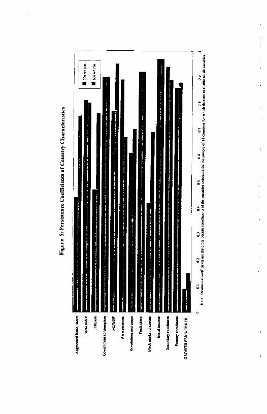
shows this explanation to be untenable: country characteristics are persistent. Figure 5 shows

persistence of country characteristics between the 60's and 70's, and between the 70's and 80's for a

sample of 45 countries for which data is available for all variables and time periods. The variables

chosen are those that appear in the classic growth regression of liarro (1991), as well as several

others common in the literature. All of the country characteristics display far higher persistence than

growth rates. Many other country characteristics, like culture and geography, must be even more

persistent.

However, some aggregate index of policy variables could still have low persistence.7 To

construct such an index, we use the variables shown in Figure 5 with a pooled time-series cross-

section regression on 10 year averages. Table 3 shows regressions using the Barro (1991) variables

with the exception of his PPI6ODEV (deviation of the relative price of investment from the sample

mean), which is not available in individual decades for a sufficient sample. (Our government

consumption variable does not exclude spending on defense and education as Barros did, due to lack

of decade data on the latter.) We allow the intercepts to vary across decades. We also perform a

'Since the persisiefice of a lines, cornbrnanon of vanables dependa on the positive or neiweve covananee among them. it is possible foran aggiqaw uidcs of counoy policies to show lower persisicnee than any of in componensi.

7

second regression with a broader set of country characteristics. The fitted values from this regression

(denoted Barro Index and Augmented Barro Index, respectively) are also far more persistent than

growth rates, as shown in Figure 5.

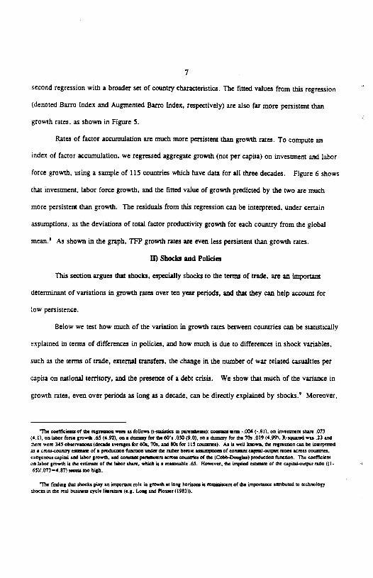
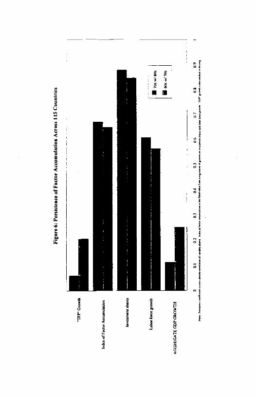
Rates of factor accumulation are much more persistent than growth razes. To compute an

index of factor accumulation, we regressed aggregate growth (not per capita) on investment and labor

force growth, using a sample of 115 countries which have data for all three decades. Figure 6 shows

that investment, labor force growth, and the fitted value of growth predicted by the two are much

more persistent than growth. The residuals from this regression can be interpreted, under certain

assumptions, as the deviations of total factor productivity growth for each country from the global

mean.C As shown in the graph, TFP growth rates are even less persistent than growth rates.

II) Shocks and Policies

This section argues that shocks, especially shocks to the terms of trade, are an important

determinant of variations in growth razes over ten year periods, and that they can help account for

low persistence.

Below we test how much of the variation in growth rates between countries can be statistically

explained in terms of differences in policies, and how much is due to differences in shock variables,

such as the terms of trade, external transfers, the change in the number of war related casualties per

capita on national territory, and the presence of a debt crisis. We show that much of the variance in

growth rates, even over periods as long as a decade, can be directly explained by shocks,° Moreover,

Thc coefficiena of thc regrninion were as follows (1-nanioci in pienuthelen): connano term -.004 (-.8 I). on Invenmient share .07(4.1), on labor force growth .65 (4.92), on a dwnzny for die 60's .030(9.0). on a dwnmy for the lOs .019 (4.99). R-sqssared was .23 andthere wise 345 obnervaaona (decade averigen for 60n. lOs. and SOs for 115 cconiws). As is well known. the rogreinion can be innapretedas a cross-counay esamate of a producOon funcoa under die rether heroic asnsnspøona of connani capitel-osispue redos across counmes.ocOgenosss capital and labor growth. end connani pssenaiers across Consoles of the (Cobb-Douglai) production fusscnon. The coelfictenton labor growth is the esturrase of the labor shase, which isa reasonable .65. However, the isriplind enonsate of the capital-output tine ((I-65)/.073 —4.87) seems aso high.

'The finding diii shocks play an important role in growth at long hofleona is reminiscent of the onporsanee anerbutad so technologyshocki an the real business cycle liternn.rre (e.g. Long and Plosser (1983)).

8

shocks indirectly influence growth by changing policy variables. Thus the low persistence of shocks.

particularly external shocks, helps explain the low persistence of growth rates.

Table 4 shows the simple correlations of three shock variables with growth rates.'° The

variables are (1) the growth in dollar export prices times the initial share of exports in GDP minus the

growth in import prices times the initial share of imports in GDP (terms of trade change); (2) the

change in war casualties per capita on national temtosy; and (3) a dummy measuring countries likely

to have a debt crisis in the 1980$." Growth is strongly correlated with terms of trade improvements

and high external debt in the 80's, and with war in the 70's (and weakly with war in the 80's).

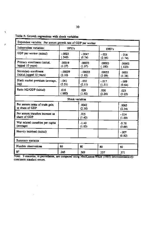
When shock variables are added to a regression with a small set of significant country

characteristics from section I, they have substantial explanatory power compared to policy variables

(Table 5). We add the three variables from the previous paragraph and, for completeness, the per

annum increase in official transfers. The partial R2 of the policy variables (enrollments, black market

premium, M2/GDP) in the 1970s was .26 and of the shocks .14, while in the 1980$ the partial R2 of

the policy variables was .10 versus .15 for shock variables.'2

The terms of trade effect is large and strongly significant in both periods. In the 1980$ a

favorable terms of trade shock of I percentage point of GDP per annum raises the growth rate by .85

percentage point per annum. Recall that GDP is measured in constant prices, so there is no direct

effect of a terms of trade shock on growth. This increase in growth is far larger than would be

created simply through the effect of the increased income on savings. Even if all the shock passed

'Our thinkAng about proper definidorn of shock ennoble, beswflnnd from the rotated work of McCasthy aM Dhazasbwsr (1991)

This isa duniosy vaflable meaasnng whether the debt in GDP run was above 50 peereasas 1990 Ia low aM middle-income counmes.We do not have compasible sasUsdos for rich cawisnea. but in a' case no rich couney expenenemi an caramel debt crisza. Date on termsof aide, exporas. imposm, caramel debt, iM GOP are from the World Bank's lnrannil datebese: date on war cumsldes ate from Sivasd(1991).

The pardui 5' of a tory er pardoulng out a is the 5' of the regression of the coniponene of y aM x orthogonal as a. This is riotthe rncvornensal it' aM the coniponeno do riot nun in the roast it'. Both petal 5¼ carbide the bUrial level of GOP.

9

into saving, and the rate of return Co capital were (optimistically) 20 percent, growth would only

increase by .2 percentage points.

Factor movements are one potential explanation of large growth effects from terms of trade

shocks.3 For example, labor or capita] might flow within the country to the sector receiving a

favorable shock, capital might flow in from abroad to the export sector, or domestic savings might

respond to improved export opportunities. In order to generate large growth effects through factor

movements, however, factors and export demand must be elastic, and terms of trade shocks must be

at least somewhat persistent.

External shock variables other than the terms of trade have smaller effects on growth, partly

reflecting substantial multicollinearity among the shocks and between shock and policy variables. The

variable for the increase in war casualties is marginally significant in the 70's but not in the 80's: we

fail to detect significant separate effects of transfers and debt crises. The magnitude of the coefficient

on the war casualty variable implies relatively modest effects of wars in most cases. Violence in

Chile associated with the overthrow of Allende and its aftermath are estimated to have cost .3

percentage points of growth per annum in the 70's. Israel's wars during the 70's are estimated to

have lowered growth during the decade by .2 percentage points per annum. Highest casualties per

capita in the sample were from the civil war in Uganda, which was estimated to have reduced growth

in the 70's by 3 percentage points per annum. Given the distribution of various shock variables (with

a few large values for casualties, transfers, and terms of trade movements) the results for individual

variables are sensitive to choice of sample.

'Another way to explain a large growth response to memo of trade nsovetssenm would be through two-gap models of the type popular inthe 1960's, in which foreign exchange xx a separate biodmg canonist on the roonensy. Amore modem explanation might be that the socialvalue of foreign exchange to higher than the private value, perhaps because it is used to import macharms that carry rxtarrt,alines, as in DeLong xrtd Surnmer (1991. 1992. 1993). Finally, the high coefficient could reflect a Keynesian aggregate demaed effect, which would be

surpnsing at such a long period length.

10

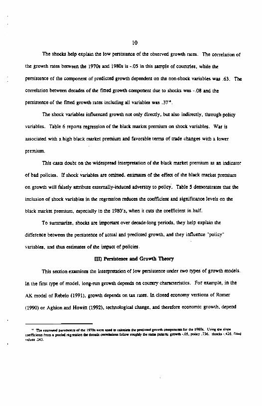
The shocks help explain the low persistence of the observed growth rates. The correlation of

the growth rates between the 1970s and 1980s is -.05 in this sample of countries, while the

persistence of the component of predicted growth dependent on the non-shock variables was .63. The

correlation between decades of the fined growth component due to shocks was -.08 and the

persistence of the fined growth rates including all variables was •37l4

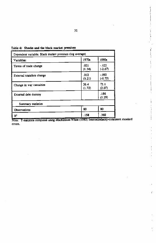
The shock variables influenced growth not only directly, but also indirectly, through policy

variables. Table 6 reports regression of the black market premium on shock variables. War is

associated with a high black market premium and favorable terms of trade changes with a lower

premium.

This casts doubt on the widespread interpretation of the black market premium as an indicator

of bad policies. If shock variables are omitted, estimates of the effect of the black market premium

on growth will falsely attribute externally-induced adversity to policy. Table 5 demonstrates that the

inclusion of shock variables in the regression reduces the coefficient and significance levels on the

black market premium, especially in the 1980's, when it cuts the coefficient in half.

To summarize, shocks are important over decade-long periods, they help explain the

difference between the persistence of actual and predicted growth, and they influence 'policy'

variables, and thus estimates of the impact of policies.

III) Pers1st and Growth Theory

This section examines the interpretation of low persistence under two types of growth models.

In the first type of model, long-run growth depends on country characteristics. For example, in the

AK model of Rebelo (1991), growth depends on tax rates. In closed economy versions of Romer

(1990) or Aghion and Howict (1992), technological change, and therefore economic growth, depend

The esarnered parunwiors of thu 1970, were used re colculute the ptodscsed growth componemm for the 9805. Using the slopecoficaenn from a pooled regression the decade canelaóons follow roughly the sante pauern growth -.05. policy .736. shocks -.426. toedv,jue .243.

11

on a countrys patent system and market size. In simple versions of these models, low persistence of

growth rates implies that random shocks are important in determining the long-run path of output. In

(he second type of model, which includes both the neoclassical model with exogenous technological

change and some models of technological diffusion, growth is a world-wide process, and country

characteristics determine the relative level of income. In these models, low persistence is consistent

with shocks of any size, and shocks may play only a minor role in determining the long-run path of

output, despite being an important determinant of variance in decade-long growth rates.

a. Modefr in Which Cowuvy Characteristics Determine Long-Run Growth

In a simple model in which country characteristics determine growth, the persistence

coefficient can be interpreted as reflecting the magnitude of variance in underlying growth rates

across countries relative to the variance of random shocks. To see this, denote the long-run growth

rate associated with the policies of country i as g1. This can be represented as the world average

growth rate, g, plus a country specific component e,, determined by country characteristics. Growth

for country i in period t equals its underlying growth rate, plus a country-specific, period-specific

shock. (A period specific aggregate shock could also be added, but would not affect the results.)

Thus.

= g+e1÷e var(c,) = a var(e) = (1)

The simplest assumption one can make is that ,and e are independent normal variables, and is

serially uncorrelated. Under this assumption, the persistence coefficient, denoted p, is

12

E(g,-g)(g, _____p 22 (2)IE(g,,_g)2 JE(g,1 _)2

0 +

This simple model of country fixed effects does not allow for changes in policy over time. However,

since policies change only slowly, it may be a reasonable approximation over periods that are not too

long. Under this model, the best forecast of a country's growth rate will be a weighted combination

of its own past growth rate and the average growth rate of all other countries.0

Under this model of fixed country effects, low persistence bounds the potential R2 that can be

achieved itt growth regressions. Even if policies were perfectly measured, and all policies and other

factors affecting growth were taken into account, the expected R2 in a thirty-year growth regression

would be only about 0.6. To see this, note that the expected R2 from regressing growth over n

periods on a perfect measure of policies that determine the country's long-nm growth rate will be

4R2(n)J = Eli - (y_!.1)h1 = -2

L (Y1)2J n2a, +r

This simplifies to

Solving t sigl eloicliOR problemgiven die best esümare of .,.

= ( 2 201,1+fl01

tl 01,,+fl01 Z

whein z is the number of counniei i n in die numberof previoun penods. flu, if them is little venison in growth rutes betweencouflolci rolauve to die venison within cowimes over nor. the country's pest growth inie will be weighted less heavily.

13

E[R2(n)] = _____

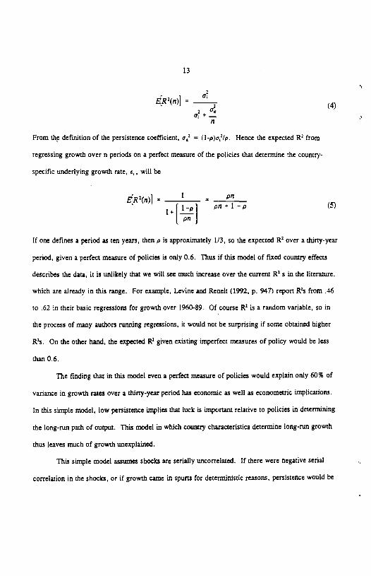
From the definition of the persistence coefficient, o = (l-p)o12/p. Hence the expected R2 from

regressing growth over n periods on a perfect measure of the policies that determine the country-

specific underlying growth rate, €, will be

R2(n)} = _____ = (If one defines a period as ten years, then p is approximately 1/3, so the expected R2 over a thirty-year

period, given a perfect measure of policies is only 0.6. Thus if this model of fixed country effects

describes the data, it is unlikely that we will see much increase over the current R5 S in the literature.

which are already in this range. For example. Levine and Renelt (1992. p. 947) report R2s from .46

to .62 in their basic regressions for growth over 1960-89. Of course R2 is a random variable, so in

the process of many authors running regressions, it would not be surprising if some obtained higher

R2s. On the other hand, the expected R2 given existing imperfect measures of policy would be less

than 0.6.

The Imding that in this model even a perfect measure of policies would explain only 60% of

variance in growth rates over a thirty-year period has economic as well as econometric implications.

In this simple model, low persistence implies that luck is important relative to policies in deterrnming

the long-run path of output. This model in which country characteristics determine long-run growth

thus leaves much of growth unexplained.

This simple model assumes shocks are serially uncorrelated. If there were negative senal

correlation in the shocks, or if growth caine in spurts for deterministic reasons, persistence would be

14

lower for given variance in underlying growth rates across countries. Thus, policies would play a

more important role in determining the long-run path of output. It is not clear why one should

expect substantial negative serial correlation over successive ten-year periods. For the spurts

hypothesis, it is interesting to note that for the countries that have four decades of data in the

Summers and Heston (1991) sample, on average around 60% of their growth from 1950 to 1988 is

achieved in the fastest-growing decade within that period. However, it is not clear whether this is

due to deterministic spurts of growth or to high random variation.

b. Models in which Worldwide Technological Progress Determines Lông-Run Growth

Under a different type of model, worldwide technological progress determines long-run

growth and country characteristics determine steady state relative levels of income. This category

includes not only the neoclassical model (Solow (1956)), but also some models of technological

diffusion. Suppose, for example, that technological progress at some rate g is generated in a few

advanced countries by a process of the type described by Romer (1990) or Aghion and Howitt (1992)

and then diffuses to other countries with lags of various lengths. Let diffusion follow the process

B X(p)(A -B)

where B is the level of technology in a backward country, p is the set of policies in that country, and

A is the level of technology in the advanced countries. Thus counthes that are further behind have

more learning potential, and countries with better policies learn faster. Setting BIB = A/A = g

implies the steady state value of B/A will be X(p)/(g+X(p))." in this model, the relative steady state

level of income is determined by policy, but except for those countries large and advanced enough to

generate a significant share of world technology, long-run growth is exogenously determined. Under

either a neoclassical model of capital accumulation or models of technological diffusion which

'For a sunlit, approach. sot Nelson and Phelps (1966). Joo,vK aurd t,ach (1991), or enhzbib and RusOchini (1993).

15

Incorporate advantages ofbackwardness, persistence depends on the distribution of countnes' incomes

relative to their steady state income.

Adding an independent normal error term to a linearized version of these models allows

persistence to be characterized. If there is a wide dispersion of distances between countries initial

incomes and their steady states, then transitional dynamics wIll dominate the effect of the random

error term. The countries furthest below their steady state will grow the fastest. Relative growth

rates will initially be highly persistent. However, as all countries approach their steady state levels of

income, persistence will fall because transitional dynamics will become less important relative to the

random error term. Asymptotically countries will converge to an ergodic distribution around the

steady state, in which persistence will be negative since countries which receive a positive random

shock one period will tend to fall back towards the steady state the next period.'7

This can be easily seen in Barro and Sala-i-Martin's linearized version of the neoclassical

model with an added random shock, but similar results hold in the diffusion model. In the

neoclassical model, Y1,.1 =—y1)

where YLs denotes log income of country i at time t.

y denotes steady state income, is a random shock, and v E (0,1) measures the speed of

adjustment to the steady state, which depends on a host of parameters, including the capital share.

Thus growth between and t+l, denoted g,, equals v(,y—y.)+s1. Iterating,

= v(y '—(y.+v(y '—y1) + + Given this, it is straightforward to write persistence as

'We consider the impact of shocks to income, but shocks to policy would have similar consequences. since these alter the stonily statelevel of income end 5anscaonaJ dyiwnics me dcscrnuoad by the difference between nitisl end the steady state level of income.

See Bane mel 5a1o-i-Mnztm (1992). n corresponds to l-c° in their riounon. This osasisple etsumea that all counirses have the some-

stonily state sod iltat there is no exogenous tecMologtcal pmgtess. bus it would be sititgborwsrd 50 genernlaze site nodel.

16

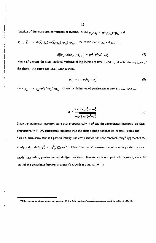
function of the cross-section variance of income. Since g. —j = v(3 —v. )+ andci I I

g.1 = v[(,—y)—v —y)—sfJ]÷p1/1 the covariance of g, and g,+1 is

=(v2_v3)a,2_vo (7)

where denotes the cross-sectional variance of log income at tune t, and a, denotes the variance of

the shock. As Barro and Sala-i-Martin show,

= (1_v)2c +g (8)

since = y+v(y —ye) +p.,,,• Given the definition of persistence as cov(g, g+1)/ac,1,

(v2_v3)a — Va2p= ______ (9)

a,I(1 _v2)cr+a

Since the numerator increases more than proportionally in o2 and the denominator increases less than

proportionally in 2, persistence increases with the cross-section variance of income. Barro and

Sala-i-Martin show that as t goes to infinity, the cross-section variance monotonicaIly9 approaches the

steady state value, o = a / (2v—v2). Thus if the initial cross-section vath.nce is greater than its

steady state value, persistence will decline over time. Persistence is asymptotically negative, since the

limit of the covariance between a countty's growth at t and at t+ I is

'This ajunus an infinbe number of counthe3. Withs finite number of counmu petisianue wowd be a rsaiom sortable.

17

(v2_v3)a2 2urn cov(g,,g,1) = _______ = (10)2v—v2 2-v

which must be negative.

Note that even if the random shocks are arbitrarily small, these models predict that persistence

will asymptotically become negative. Under this model, a country's time path of income could be

determined almost completely by worldwide technological change and its policies, but if it were close

to its steady state income a large percentage of the time series variance in its growth rate would be

explained by random shocks. In this case the growth rate would just represent fluctuations around a

steady state income.

This model could be generalized by allowing each country to have its own steady state level

of income depending on policies, and by allowing for exogenous technological change. In this case,

persistence depends not on variance of income, but on variance in the gap between actual income and

steady state income relative to the level of technology. If countries vary greatly in their distance from

their relative steady states, persistence will be high. The countries far below their relative steady

state income will initially have persistently high growth rates. As they approach the steady state.

their growth rate will fall.

Asymptotically, there is a sharp distinction between models in which country characteristics

determine long-run growth and models in which country characteristics determine relative steady state

income. However, if countries are far from their steady states, models in which country

characteristics determine income look similar to those in which country characteristics determine

growth rates.

One difficulty with this type of model is that it does not explain why we observe countries

outside the ergodic distribution around the steady state. Barro and Sala-i-Martin have suggested

18

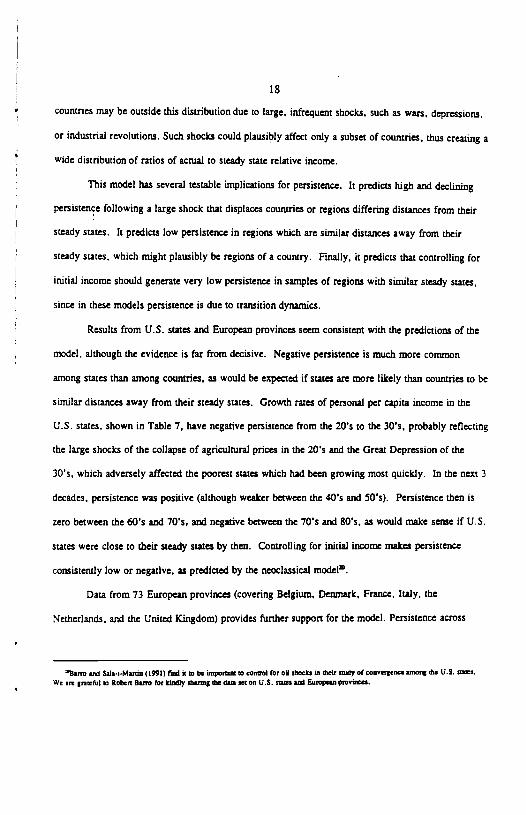
countnes may be outside this distribution due to large, infrequent shocks, such as wars, depressions,

or industrial revolutions. Such shocks could plausibly affect only a subset of counthes, thus creating a

wide distribution of ratios of actual to steady state relative income.

This model has several testable implications for persistence. It predicts high and declining

persistence following a large shock that displaces countries or regions differing distances from their

steady states. It predicts low persistence in regions which are similar distances away from their

steady states, which might plausibly be regions of a country. Finally, it predicts that controlling for

initial income should generate very low persistence in samples of regions with similar steady states,

since in these models persistence is due to transition dynamics.

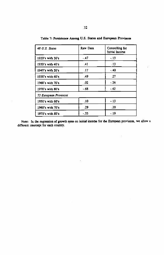
Results from U.S. states and European provinces seem consistent with the predictions of the

model, although the evidence is far from decisive. Negative persistence is much more common

among states than among countries, as would be expected if states are more likely than countries to be

similar distances away from their steady states, Growth rates of personal per capita income in the

U.S. states, shown in Table 7, have negative persistence from the 20's to the 30's. probably reflecting

the large shocks of the collapse of agricultural prices in the 20's and the Great Depression of the

3D's, which adversely affected the poorest states which had been growing most quickly. In the next 3

decades, persistence was positive (although weaker between the 40's and 50's). Persistence then is

zero between the 60's and 70's, and negative between the 70's and 80's, as would make sense if U.S.

states were close to their steady states by then. Controlling for initial income makes persistence

consistently low or negative, as predicted by the neoclassical models.

Data from 73 European provinces (covering Belgium, Denmark, France, Italy, the

Netherlands, and the United Kingdom) provides further support for the model. Persistence across

e8a,To and Saia+Manm (1991) fInd it to be important to conuol (or od shocks in their study of conver5eoce antong the U.S. stutos.

We ire gratcitsi to Robert Bamo (or kindiy sharing the datu set on U.S. stunu and Eiuopeinprootncu.

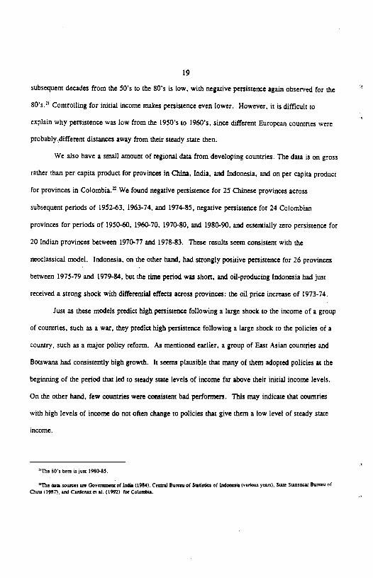
19

subsequent decades from the 50's to the 80's is low, with negative persistence again observed for the

80's. Controlling for initial income makes persistence even lower. However, it is difficult to

explain why persistence was low from the 1950's to 1960's, since different European countries were

probablydifferent distances away from their steady state then.

We also have a small amount of regional data from developing countries. The data is on gross

rather than per capita product for provinces in China, India, and Indonesia, and on per capita product

for provinces in Colombia.n We found negative persistence for 25 Chinese provinces across

subsequent periods of 1952-63, 1963-74, and 1974-85, negative persistence for 24 Colombian

provinces for periods of 1950-60, 1960-70, 1970-80, and 1980-90, and essentially zero persistence for

20 Indian provinces between 1970-77 and 1978-83. These results seem consistent with the

neoclassical model. Indonesia, on the other hand, had strongly positive persistence for 26 provinces

between 1975-79 and 1979-84, but the time period was short, and oil-producing Indonesia had just

received a strong shock with differential effects across provinces: the oil price increase of 1973-74.

Just as these models predict high persistence following a large shock to the income of a group

of countries, such as a war, they predict high persistence following a large shock to the policies of a

country, such as a major policy reform. As mentioned earlier, a group of East Asian countries and

Botswana had consistently high growth. It seems plausible that many of them adopted policies at the

beginning of the period that led to steady state levels of income far above their initial income levels.

On the other hand, few countries were consistent bad performers. This may indicate that countries

with high levels of income do not often change to policies that give them a low level of steady state

income.

The 80s hcr ,s just 1980-55.

The da souitcs u Gocrnmem of India (1984). Ceiin.i Burtau of sstnsocs of 1ndoias,a (various yevs), Stab Siaasncal Burouu ofChina (1987). and Cardersas es al. (1992) for Colombia.

20

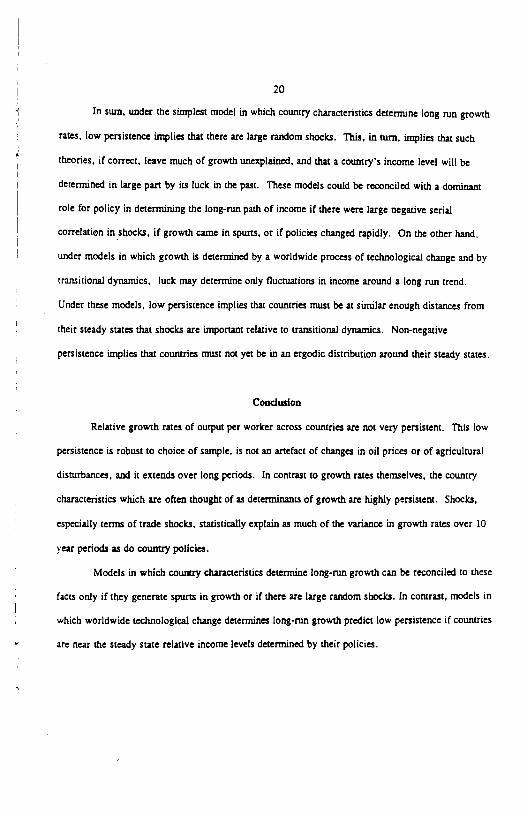
In sum, under the simplest model in which country characteristics determine long run growth

rates, low persistence implies that there are large random shocks. This, in turn, implies that such

theories, if correct, leave much of growth unexplained, and that a country's income level will be

determined in large part by its luck in the past. These models could be reconciled with a dominant

role for policy in determining the long-run path of income if there were large negative serial

correlation in shocks, if growth caine in spurts, or if policies changed rapidly. On the other hand.

under models in which growth is determined by a worldwide process of technological change and by

transitional dynamics, luck may determine only fluctuations in income around a long run trend.

Under these models, low persistence implies that countries must be at similar enough distances from

their steady states that shocks are important relative to transitional dynamics. Non-negative

persistence implies that countries must not yet be in an ergodic distribution around their steady states.

Conclusion

Relative growth rates of output per worker across countries are not very persistent. This low

persistence is robust to choice of sample, is not an artefact of changes in oil prices or of agricultural

disturbances, and it extends over long periods. In contrast to growth rates themselves, the country

characteristics which are often thought of as determinants of growth are highly persistent. Shocks,

especially terms of trade shocks, statistically explain as much of the variance in growth rates over 10

year periods as do country policies.

Models in which country characteristics determine long-run growth can be reconciled to these

facts only if they generate spurts in growth or if there are large random shocks. In contrast, models in

which worldwide technological change determines long-run growth predict low persistence if countries

are near the steady state relative income levels determined by their policies.

21

The finding that much variation in growth rates is due to random shocks should induce

caution in attributing high growth rates to good policy (or to a good 'work ethic'). Just as a baseball

star is dubbed a clutch hitter after a lucky hit, some so-called economic miracles are likely due to

random variation.

22

BIBLIOG1t4Jy

Aghion, P. and P. Howitt, 1992, A model of growth through creative destruction, Econometrica 60.323-51.

Alesina, A. and D. Rodrik, 1991, Distributive politics and economic growth, NBERWorking Paper3668.

Barro, R.J., 1991, Economic growth in a cross section of countries, Quarterly Journal of Economics.106: 407-43.

—. 1990, Government spending in a simple model of endogenotis growth, Journal of PoliticalEconomy 98,S103-S125.

and X. Sala-I-Martin, 1992, Convergence, Journal of Political Economy, 100: 223-51.

— and _______, 1991, Economic growth and convergence across the United States, BrookingsPapers on Economic Activity 1, 107-82.

and H.C. Wolf, 1989, Data appendix for economic growth in a cross section of counthes,rnimeo, Harvard University and MIT.

and J.W. Lee, 1993, International comparisons of educational attainment, Journal of MonetazyEconomics, this issue.

Benhabib, Jess and Rustichini, Aldo. 1993, 'Follow the Leader: On Growth and Diffusion", workingpaper, C.V. Starr Center for Applied Economics. NYU,

Borjas, GJ., 1992, Ethnic capital and intergenerational mobility, Quarterly Journal of Economics107, 123-50.

Cardenas, M., A. Ponton, and J.P. Trujillo,1992, Convergencia, Crecimiento, y Migraciones Inter-departmentales: Colombia 1950-89, mixneo, Fedesarrollo (Bogota).

Central Bureau of Statistics, various years, Statistical yearbook of Indonesia, Government ofIndonesia (Jakarta)

Dc Long, J.B., 1988, Productivity growth, convergence, and welfare: comment, American EconomicReview 78:5, 1138-1154.

Dc Long, J.B. and L.H. Summers, 1991, Equipment, investment, relative prices, and economicgrowth, Quarterly Journal of Economics, CVI: 2, 445-502.

— and , 1992, Equipment investment and economic growth: how robust is the nexus?,Brookings Papers on Economic Activity 2, 157-211.

23

and —, 1993, How strongly do developing economies benefit from equipment investment?,Journal of Monetary Economics, this issue.

Easterly, W., 1993, How much do distortions affect growth?, Journal of Monetary Economics,forthcoming.

and S. Rebelo, 1993, Fiscal policy and economic growth: an empirical investigation, Journal ofMonetary Economics, this issue.

Fischer. S., 1993, Macroeconomic factors in growth, Journal of Monetary Economics, this issue.

1991, Growth, macroeconomics and development, in 0. Blanchard and S. Fischer, eds..NBER Macroeconomics Annual 1991 (MIT Press: Cambridge, MA), 329-364.

1987. Economic growth and economic policy, in: V. Corbo, M. Goldstein. and M. Khan.eds.. Growth-oriented Adjustment Programs, (IMF and World Bank, Washington, D.C.),151-78.

Gelb, A.}L, 1989. Financial policies, growth, and efficiency, World Bank PPR Working Paper 202

(Washington, DC).

Government of India, 1984, Estimates of state domestic product 1960-61 to 1982-83 (New Delhi:Government of India)

Greenwood, J. and B. Jovanovic, 1990, Financial development, growth, and the distribution ofincome, Journal of Political Economy 98, 1076-1107.

Grossman, G. and E. Helpinan, 1991, Innovation and growth: technological competition in the worldeconomy, MIT Press (Boston. Massachusetts).

Harrison, A., 1991, Openness and growth: a time-series, cross-country analysis for developingcountries, World Bank PRE Working Paper 809 (Washington, DC).

Jones, L. and R. Manuelli, 1990, A convex model of equilibrium growth. Journal of PoliticalEconomy 98 5, 1008-38.

Jovanovic, B. and S. Lach, 1991, The diffusion of technology and inequality among nations, NBERWorking Paper 3732.

King, R. and S. Rebelo, 1990, Public policy and economic growth: developing neoclassicalimplications. Journal of Political Economy 98. S126-l50.

King, R. and R. Levine. 1993, Finance, entrepreneurship, and development. Journal of MonetaryEconomics, this issue.

Levine, R., 1991. Stock markets, growth and policy, Journal of Finance, 46:1445-65.

24

— and D. Renelt, 1992, A sensitivity analysis of cross-country growth regressions, AmericanEconomic Review, 82:4, 942-963.

and —, 1991, Cross-country studies of growth and policy: some methodological.conceptual, and statistical problems, World Bank PRE Working Paper 608 (Washington, DC).

Long, I. and Plosser, C. Real business cycles. Journal of Political Economy, February 1983, 91:1,39-69.

Lucas, R.E, 1988, On the mechanics of economic development, Journal of Monetary Economics 22,3-42.

MacKinnon, 1G. and H. White, 1985, Some heteroskedasticity-consistent covariance matrixestimators with improved finite sample properties, Journal of Econometrics (Netherlands) 29,305-25.

Maddison, A., 1989, The World Economy in the 20th Century (OECD, Paris).

McCarthy, F.D, and A. Dhareshwar, 1991, Economic shocks and the global environment, WorldBank, rnimeo.

Murphy, K., A. Shleifer, and R. Vishny, 1991, The allocation of talent: implications for growth,Quarterly Journal of Economics, CVI:2, 503-530.

Nelson. R. and Phelps, E. 1966. lnvestment in Humans. Technological Diffusion, and EconomicGrowth American Economic Review Papers and Proceedings, pp. 69-75.

North. D.C., 1989. Institutions and economic growth: A historical introduction, World Development17:9, 1319-1332.

Persson, T. and 0. Tabellini, 1991, Is inequality harmful for growth? Theory and evidence. NBERWorking Paper 3599.

Quah. D. 1993, Empirical cross-section dynamics in economic growth, European Economic Review,37, 426-34.

Rebelo, S., 1991. Long run policy analysis and long run growth, Journal of Political Economy. 99,500-21.

Rivera-Batiz, L.A. and P.M. Romer, 1991, International trade with endogenous technological change.European Economic Review (Netherlands) 35. 971-1004.

Romer, P. 1990. Endogenous technological change, Journal of Political Economy 98. S71-S102.

—, 1989, What determines the rate of growth of technological change?, World Bank PPRWorking Paper No. 279. (Washington. DC).

25

—, 1987, Crazy explanations for the productivity slowdown, in S. Fischer ed. NBERMacroeconomics Annual 1987 (MIT Press: Cambridge, MA), 163-202.

—' 1986, Increasing returns and long-run growth, Journal of Political Economy 94, 1002-1037.

Solow, R. 1956, A contribution to the theory of economic growth, Quarterly Journal of Economics70, 65-94.

Sivard, R.L., 1991, World military and social expenditure (Leesburg VA: WMSE Publications)

State Statistical Bureau of China, 1987, National Income Statistical Data Collection 1949-85 (ChinaStatistics Press (Beijing)) (in Chinese)

Stockrnan, A., Sectoral and national aggregate disturbances to industhal output in seven Europeancountries, Journal of Monetary Economics 8, 387-393.

Summers, R. and A. Heston, 1991, The Penn World Table (Mark 5): An Expanded Set ofInternational Comparisons 1950-88, Quarterly Journal of Economics, CVI:2, 327-368.

Young, A., 1991, Learning by doing and the dynamic effects of international trade, Quarterly Journalof Economics, CVI: 2, 369-406.

26

Table 1: Simple and raniccorrelations of growth rateacross periods

60's with 70's correlationcoefficient:

70's with 80's correlationcoefficient:

Sample: Sample Size: Simple Rank Simple Rank

All Countries 100 .212 .233 .313 .157

All non-oil 89 .153 .227 .301 .187

OECD 22 .729 .701 .069 .086

Developingcountries, non-oil

67 .099 .150 .332 .251

27

Table 2: Cross-Sector rank correlations ofper worker owti rates

Decades

60's 70's SO's

Agriculture, Industry .09 .29 14

Agriculture, Services .10 .45 31

Industry, Services .20 .57 .27

Sample Size 67 67 39

28

Table 3: Pooled Cross-section Time Series Regressions of Long-Term Growthon Policy Variables with Decade Averages

Dependent Variable: Growth Rate of GDP Per Worker"

Independent Variables: Barroregression

AugmentedBarroregression

GDP Per Worker (Initial) -.0 13(-2.62)

-.0 12(-2.93)

Primary Enrollment (Initial Lagged 10 years) .019(2.16)

.013(1.63)

Secondary Enrollment (Initial Lagged 10 years) .026(2.12)

.0097(0.86)

Assassinations per million (Avg) -.013(-1.19)

-.013(1.40)

Revolutions and coups (Avg) -.0029(-0.52)

.004(0.90)

Share of Government Consumption in GDP (Avg) -.0089(-0.29)

.035(1.18)

Log Black Market Premium (Avg) -.038(-3.74)

Inflation (Avg) .0042(0.92)

Share of trade in GDP (Initial) -.0059(1.18)

Ratio M2/GDP (Initial) .025(3.88)

Summary Statistics

N 135 135

R2 .43 .58

Notes:1 Absolute values of t-stazistjcs calculated with MacKinnon-Whjte (1985)heteroskedasticity consistent standard errors in parentheses. Dependent variable isthe least-squares growth rate of Summers-Heston (1991) output per worker.2/ Pooled regression has separate decade constant terms, nor reported.

29

Table 4: Simple correlatioos of growth and shocks

Correlation of growthwith:

1970's 1980's

Terms of tradechange

.10 .45

Change in warcasualties

-.31 -.12

Dummy for highexternal debt, 1980

-. 19

rsigmncant at 10% levelsigrnficant at 5% level

significant at 1% level

30

Table 5: Growth regrassiOns with shock variablea

Dependent variable: Per annum growth rate of GDP per worker

Independent variables: 1970's 1980's

GDP per worker (initial).

-.0023(.349)

-.0047(0.74)

-.021(2.06)

-.0 16

(1.74)Primary enrollment (initial,lagged 10 years)

.00019(1.27)

.00033(1.97)

.00003(.180)

.00002(.123)

Secondary enrollment(initial.lagged 10 years)

-.00039(2.10)

-.00033(1.83)

.00053(2.09)

.0003(1.38)

Black market premium (average,log)

-.041(2.51)

-.032(2.11)

-.0 17

(1.51)-.009(0.64)

Ratio M2/GDP (initial) .016(.980)

.026(1.92)

.030(2.29)

.023(2.03)

Shock variables

Per annum terms of trade gainas share of GDP

.0042(2.36)

.0085(2.24)

Per annum transfers increase asshare ofGDP

.015(1.43)

-.014(1.69)

War related casualties per capita(average)

-1.40(1.83)

-0.78(0.69)

Heavily indebted (initial) -.007(0.82)

Summary statistics

Number observations 80 80 80 80

.265 .371oLe: i-statistics, in parentheses, are computed using macrunnon-w ute (19) fleterosKeast1city-

consistent standard errors.

31

Table 6: Shocks and the black market prnium

Dependent variable: Black market premium (log average)

Variables: 1970s 1980s

Terms of trade change .021(1.34)

-.122(-2.67)

External transfers change .012(0.21)

-.092(-0.75)

Change in war casualties 36.4(1.72)

73.1(2.07)

External debt dummy .186(1.29)

Summary statistics

Observations 80 80

R2 .158 .360

[ole: T-staflstlcs COTTIPUICO using M3C1flDOfl-Wh1t ( 985) he osdacity-COnsiStent standarderrors.

32

Table 7: Persistence Among U.S. States and European Provinces

48 U.S. Stcies Raw Data Controlling forInitial Income

1920's with 30's -.47 -.13

1930's with 40's .41 13

1940's with 50's .17 -.40

1950's with 60's .49 .27

1960's with 70's .02 -.26

1970's with 80's -.68 -.62

73 European Provinces

1950's with 60's .10 -.13

1960's with 70's .29 .20

1970's with 80's -.33 -.19

Note: In the regression of growth rates on initial income for the European provinces, we allow adifferent intercept for each country.

Figure 1: Per Worker Growth Ratea Per Year, 1960-73and 1974-88

I CPV ___ IoH I0,

ONI0*1w__________ o.

3g1 .ui I IcOn

• PAK

BDI 1-KA PNVITAavoNfl

LSL WA 17J.GO e. cDCU TU

______ PIA DZAwzMfln aen __ — —SOM P 4

Kf

o Average (0.6)

'flITO-2.7r

I NGA ___ 'A''lCD Is1

"F

I Average 3.10I=1 y0I

Guy

B000m 0.4 5.5 - Top TenthTenth Growth 1960-73

Vote: G,-owth razes are leas-squarts growth per worker for each coviizry for penods shoveThe three letter World Bankcode., for counny names, which are also used in Summers and

Heston (199/) and Barro and Wolf (1989). are used for each poEnt.

14

12

C

10 4

Figu

re 2

: C

orre

latio

ns o

f Per

Wor

ker G

row

th R

ates

Acr

oss P

erio

ds b

y L

engt

h of

Pe

riod

Cor

rela

tion

Coe

ffici

ent

Hol

e: e

ach c

unct

atio

n sh

own

is th

e av

erag

e of a

ll co

rrel

atio

ns a

cros

s sa

hseq

aent

per

iods

of t

hat l

engt

h ov

er 1

960-

88,

0 01

02

03

04

0.

5 06

0.

7 08

00

Figure 3: Persistence of per capita growth rates acrosssuccessive 30-year periods, 1870-1988

J.(I9)O.9 I.U) (I93G. I94I)5%

(l79. U

U• • B.J (I-$. l93O.-9)(jUlO-99 .29)

/• 1G(i59I9U)

C..(l9-9. 19i-S9) S U• UUU••• j._• •

• U.I9O49)

U USAC I}O-5 9G-SI)•1%

. U

ç 0%ly(ll.!!9)

-1%Chlt(I9O-9. 960-fl)

960-29)— (lI)60, I29)

-2%

-2% •I% 0% 1% 2% 3% 4% 5%

Growth In first 30-yenr perIod

Noi

cs: T

he s

ampl

e siz

e is

69

coun

trie

s in

the

60s

with

lOs

coirc

latio

n.

and

40 c

ount

ries

in th

e lO

s w

ith 8

0s c

orre

latio

n.

Gro

wth

in t

he d

eriv

ed a

ggre

gate

GD

P p

er w

orke

r ha

s ra

nk

corr

elat

ion

coef

licie

nla

or.2

7 and

.35.

resp

ectiv

ely

• lOs

with

SO

s

(sO

s w

ith lO

s

Figu

re 4:

Ran

k Cor

rela

tion

Coe

ffic

ient

s of P

er W

orke

r Gro

wth

by

Sect

or

Ser

vice

s

Indu

stry

Agr

icul

ture

-o 2

o

02

04

Ran

k co

rrel

atio

n co

effic

ient

acr

osa d

ecad

nu

0.6

OS

Ca

I.'aCa

C-

.0U

00UI-00'a'a

'a0U'aCa0'a01

'a0..

'(C

'aI.02

I8

0I8

I8

I—e02

22

§

—

0z

I I I I I I

I I

I12

Fig

ure

6: P

ersi

sten

ce of

Fact

or A

ccum

ulat

ion

Acr

oss

15 C

ount

ries

TFP

Gro

wth

Inde

x of F

acio

r Acc

umui

thon

Inve

stm

ent th

arc5

Lab

or Fo

rce g

row

th

AG

GR

EG

AT

I GD

P G

RO

WT

H

0 D

I 02

03

0.

4 0.

5 06

07

08

09

N

ki p

......

. ...s

v..

.w...

.. g .w

.öi.

.v...

. l.a

.. S

r..t..

.1...

,. th

. Ins .

il.. t

o.. a

.....

... .A

oo.1

k o.

. ,.o

..a a

... .5

a...

I....

....

a. i.

r g.o

..a ..

a.. ,..

tS n

M..

I

I • lO

s w

I S

Os

60s

wi

lOs