goodness-of-fittest …leemis/2008commst.pdfd n=maxd +d − although the test statistic d n is easy...

Communications in Statistics—Simulation and Computation®, 37: 1396–1421, 2008Copyright © Taylor & Francis Group, LLCISSN: 0361-0918 print/1532-4141 onlineDOI: 10.1080/03610910801983160

Goodness-of-Fit Test

The Distribution of the Kolmogorov–Smirnov,Cramer–vonMises, and Anderson–DarlingTest Statistics for Exponential Populations

with Estimated Parameters

DIANE L. EVANS1, JOHN H. DREW2,AND LAWRENCE M. LEEMIS2

1Department of Mathematics, Rose–Hulman Institute of Technology,Terre Haute, Indiana, USA2Department of Mathematics, The College of William & Mary,Williamsburg, Virginia, USA

This article presents a derivation of the distribution of the Kolmogorov–Smirnov,Cramer–von Mises, and Anderson–Darling test statistics in the case of exponentialsampling when the parameters are unknown and estimated from sample data forsmall sample sizes via maximum likelihood.

Keywords Distribution functions; Goodness-of-fit tests; Maximum likelihoodestimation; Order statistics; Transformation technique.

Mathematics Subject Classification 62F03; 62E15.

1. The Kolmogorov–Smirnov Test Statistic

The Kolmogorov–Smirnov (K–S) goodness-of-fit test compares a hypothetical orfitted cumulative distribution function (cdf) F̂ �x� with an empirical cdf Fn�x� inorder to assess fit. The empirical cdf Fn�x� is the proportion of the observationsX1� X2� � � � � Xn that are less than or equal to x and is defined as:

Fn�x� =I�x�

n�

where n is the size of the random sample and I�x� is the number of Xi’s less thanor equal to x.

Received July 23, 2007; Accepted February 12, 2008Address correspondence to Lawrence M. Leemis, Department of Mathematics, The

College of William & Mary, Williamsburg, VA 23187, USA; E-mail: [email protected]

1396

Test Statistics for Exponential Populations with Estimated Parameters 1397

The K–S test statistic Dn is the largest vertical distance between Fn�x� and F̂ �x�for all values of x, i.e.,

Dn = supx

��Fn�x�− F̂ �x��

The statistic Dn can be computed by calculating (Law and Kelton, 2000, p. 364)

D+n = max

i=1�2��n

{i

n− F̂ �X�i��

}� D−

n = maxi=1�2��n

{F̂ �X�i��−

i− 1n

}�

where X�i� is the ith order statistic, and letting

Dn = max�D+n � D

−n ��

Although the test statistic Dn is easy to calculate, its distribution ismathematically intractable. Drew et al. (2000) provided an algorithm for calculatingthe cdf of Dn when all the parameters of the hypothetical cdf F̂ �x� are known(referred to as the all-parameters-known case). Assuming that F̂ �x� is continuous,the distribution of Dn, where X1� X2� � � � � Xn are independent and identicallydistributed (iid) observations from a population with cdf F�x�, is a function of n, butdoes not depend on F�x�. Marsaglia et al. (2003) provided a numerical algorithmfor computing Pr�Dn ≤ d�.

The more common and practical situation occurs when the parameters areunknown and are estimated from sample data, using an estimation technique suchas maximum likelihood. In this case, the distribution of Dn depends upon both nand the particular distribution that is being fit to the data. Lilliefors (1969) providesa table (obtained via Monte Carlo simulation) of selected percentiles of the K–Stest statistic Dn for testing whether a set of observations is from an exponentialpopulation with unknown mean. Durbin (1975) also provides a table (obtainedby series expansions) of selected percentiles of the distribution of Dn. This articlepresents the derivation of the distribution of Dn in the case of exponential samplingfor n = 1, n = 2, and n = 3. Additionally, the distribution of the Cramer–von Misesand Anderson–Darling test statistics for n = 1 and n = 2 are derived in Sec. 2.Two case studies that analyze real-world data sets (Space shuttle accidents andcommercial nuclear power accidents), where n = 2 and the fit to an exponentialdistribution is important, are given in Sec. 3. Future work involves extending theformulas established for the exponential distribution with samples of size n = 1� 2,and 3 to additional distributions and larger samples. For a summary of the literatureavailable on these test statistics and goodness-of-fit techniques (including tabledvalues, comparative merits, and examples), see D’Agostino and Stephens (1986).

We now define notation that will be used throughout the article. Let Xbe an exponential random variable with probability distribution function (pdf)f�x� = 1

�e−x/� and cdf F�x� = 1− e−x/� for x > 0 and fixed, unknown parameter

� > 0. If x1� x2� � � � � xn are the sample data values, then the maximum likelihoodestimator (MLE) �̂ is:

�̂ = 1n

n∑i=1

xi�

1398 Evans et al.

We test the null hypothesis H0 that X1� X2� � � � � Xn are iid exponential(�) randomvariables.

1.1. Distribution of D1 for Exponential Sampling

If there is only n = 1 sample data value, which we will call x1, then �̂ = x1.Therefore, the fitted cdf is:

F̂ �x� = 1− e−x/�̂ = 1− e−x/x1 x > 0�

As shown in Fig. 1, the largest vertical distance between the empirical cdf F1�x� andF̂ �x� occurs at x1 and has the value 1− 1/e, regardless of the value of x1. Thus, thedistribution of D1 is degenerate at 1− 1/e with cdf:

FD1�d� =

{0 d ≤ 1− 1/e

1 d > 1− 1/e�

1.2. Distribution of D2 for Exponential Sampling

If there are n = 2 sample data values, then the maximum likelihood estimate (mle)is �̂ = �x1 + x2�/2, and thus the fitted cdf is:

F̂ �x� = 1− e−x/�̂ = 1− e−2x/�x1+x2� x > 0�

A maximal scale invariant statistic (Lehmann, 1959, p. 215) is:

x1x1 + x2

�

Figure 1. The empirical and fitted exponential distribution for one data value x1, whereD−

1 = 1− 1/e and D+1 = 1/e. (Note: The riser of the empirical cdf in this and other figures

has been included to aid in comparing the lengths of D−1 and D+

1 ).


The associated statistic which is invariant to re-ordering is:

y = x�1�

x�1� + x�2��

where x�1� = min�x1� x2�, x�2� = max�x1� x2�, and 0 < y ≤ 1/2 since 0 < x�1� ≤ x�2�.The fitted cdf F̂ �x� at the values x�1� and x�2� is:

F̂ �x�1�� = 1− e−2x�1�/�x�1�+x�2�� = 1− e−2y�

and

F̂ �x�2�� = 1− e−2x�2�/�x�1�+x�2�� = 1− e−2�1−y��

It is worth noting that the fitted cdf F̂ �x� always intersects the second riser ofthe empirical cdf F2�x�. This is due to the fact that F̂ �x�2�� can range from 1− 1/e �0�6321 (when y = 1/2) to 1− 1/e2 � 0�8647 (when y = 0), which are both includedin the second riser’s extension from 0.5 to 1. Conversely, the fitted cdf F̂ �x� mayintersect the first riser of the empirical cdf F2�x�, depending on the value of y. When0 < y ≤ ln�2�

2 � 0�3466, the first riser is intersected by F̂ �x� (as displayed in Fig. 2),but when ln�2�

2 < y ≤ 1/2, F̂ �x� lies entirely above the first riser (as subsequentlydisplayed in Fig. 6).

Define the random lengths A, B, C, and D according to the diagram in Fig. 2.With y = x�1�/�x�1� + x�2��, the lengths A, B, C, and D (as functions of y) are:

A = �1− e−2y�− 0 = 1− e−2y 0 < y ≤ 1/2�

Figure 2. The empirical and fitted exponential distribution for two data values x�1� and x�2�.In this particular plot, 0 < y ≤ ln�2�

2 , so the first riser of the empirical cdf F2�x� is intersectedby the fitted cdf F̂ �x�.

1400 Evans et al.

B =∣∣∣∣12 − �1− e−2y�

∣∣∣∣ =e−2y − 1

20 < y ≤ ln�2�

2�

12− e−2y ln�2�

2< y ≤ 1/2�

C = �1− e−2�1−y��− 12= 1

2− e−2�1−y� 0 < y ≤ 1/2�

D = 1− �1− e−2�1−y�� = e−2�1−y� 0 < y ≤ 1/2�

where absolute value signs are used in the definition of B to cover the case in whichF̂ �x� does not intersect the first riser.

Figure 3 is a graph of the lengths A, B, C, and D plotted as functions of y,for 0 < y ≤ 1/2. For any y ∈ �0� 1/2�, the K–S test statistic is D2 = max�A� B�C�D�.Since the length D is less than max{A, B, C} for all y ∈ �0� 1/2�, only A, B, and C

are needed to define D2.Two particular y values of interest (indicated in Fig. 3) are y∗ and y∗∗ since:

1. for 0 < y < y∗, B = max�A� B�C�D�;2. for y∗ < y < y∗∗, C = max�A� B�C�D�;3. for y∗∗ < y ≤ 1/2, A = max�A� B�C�D�;4. B�y∗� = C�y∗� and C�y∗∗� = A�y∗∗�.

The values of y∗, y∗∗, C�y∗�, and C�y∗∗� are given below:

• The smallest value y∗ in �0� 1/2� such that B�y∗� = C�y∗� is:

y∗ = 1+ 12ln(12− 1

2

√1− 4

e2

)� 0�0880�

Figure 3. Lengths A, B, C, and D from Fig. 2 for n = 2 and 0 < y ≤ 1/2.


which results in

C�y∗� = 12

√1− 4

e2� 0�3386�

• The only value y∗∗ in �0� 1/2� such that A�y∗∗� = C�y∗∗� is:

y∗∗ = 1+ 12ln(14

√1+ 16

e2− 1

4

)� 0�1821�

which results in

C�y∗∗� = 34− 1

4

√1+ 16

e2� 0�3052�

Thus, the largest vertical distance D2 is computed using the length formula forA�Y�, B�Y�, or C�Y� depending on the value of the random variable Y = X�1�/�X�1� +X�2��, i.e.,

D2 =

B�Y� 0 < Y ≤ y∗

C�Y� y∗ < Y ≤ y∗∗

A�Y� y∗∗ < Y ≤ 1/2�

1.2.1. Determining the Distribution of Y = X�1�/�X�1� + X�2��. Let X1� X2 be arandom sample drawn from a population having pdf

f�x� = 1�e−x/� x > 0�

for � > 0. In order to determine the distribution of D2, we must determinethe distribution of Y = X�1�/�X�1� + X�2��, where X�1� = min�X1� X2� and X�2� =max�X1� X2�.

Using an order statistic result from Hogg et al. (2005, p. 193), the joint pdf ofX�1� and X�2� is:

g�x�1�� x�2�� = 2! · 1�e−x�1�/� · 1

�e−x�2�/� =

(2�2

)e−�x�1�+x�2��/� 0 < x�1� ≤ x�2��

In order to determine the pdf of Y = X�1�/�X�1� + X�2��, define the dummytransformation Z = X�2�. The random variables Y and Z define a one-to-onetransformation that maps � = ��x�1�� x�2�� 0 < x�1� ≤ x�2�� to � = ��y� z� � 0 < y ≤1/2� z > 0�. Since x�1� = yz/�1− y�, x�2� = z, and the Jacobian of the inversetransformation is z/�1− y�2, the joint pdf of Y and Z is:

h�y� z� = 2�2

e−�z+yz/�1−y��/� ·∣∣∣∣ z

�1− y�2

∣∣∣∣ = 2z�2�1− y�2

e−z/�1−y�� 0 < y ≤ 1/2� z > 0�

1402 Evans et al.

Integrating the joint pdf by parts yields the marginal pdf of Y :

fY �y� =2

�2�1− y�2

∫ �

0ze−z/�1−y�� dz = 2 0 < y ≤ 1/2�

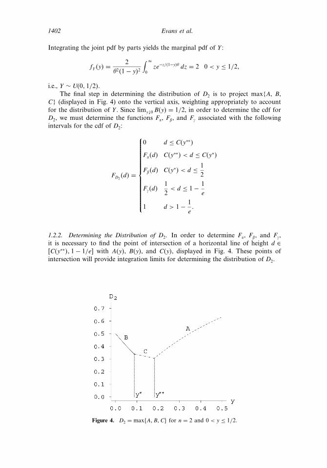
i.e., Y ∼ U�0� 1/2�.The final step in determining the distribution of D2 is to project max{A, B,

C} (displayed in Fig. 4) onto the vertical axis, weighting appropriately to accountfor the distribution of Y . Since limy↓0 B�y� = 1/2, in order to determine the cdf forD2, we must determine the functions F, F, and F� associated with the followingintervals for the cdf of D2:

FD2�d� =

0 d ≤ C�y∗∗�

F�d� C�y∗∗� < d ≤ C�y∗�

F�d� C�y∗� < d ≤ 12

F��d�12< d ≤ 1− 1

e

1 d > 1− 1e�

1.2.2. Determining the Distribution of D2. In order to determine F, F, and F�,it is necessary to find the point of intersection of a horizontal line of height d ∈�C�y∗∗�� 1− 1/e� with A�y�, B�y�, and C�y�, displayed in Fig. 4. These points ofintersection will provide integration limits for determining the distribution of D2.

Figure 4. D2 = max�A� B�C� for n = 2 and 0 < y ≤ 1/2.


Solving B�y� = d, where d satisfies B�y∗� ≤ d < 1/2 yields:

y = −12ln(d + 1

2

)�

Solving C�y� = d, where d satisfies C�y∗∗� ≤ d ≤ C�y∗�, yields:

y = 1+ 12ln(12− d

)�

Finally, solving A�y� = d where d satisfies A�y∗∗� ≤ d ≤ 1− 1e, yields:

y = −12ln�1− d��

The following three calculations yield the limits of integration associated withthe functions F, F, and F�. For C�y

∗∗� < d ≤ C�y∗�:

FD2�d� = F�d�

= Pr�D2 ≤ d�

=∫ − 1

2 ln�1−d�

1+ 12 ln� 12−d�

fY �y� dy

= −2− ln��1/2− d��1− d��

For C�y∗� < d ≤ 1/2:

FD2�d� = F�d�

= Pr�D2 ≤ d�

=∫ − 1

2 ln�1−d�

− 12 ln�d+ 1

2 �fY �y�dy

= ln(d + 1/21− d

)�

For 1/2 < d ≤ 1− 1/e:

FD2�d� = F��d�

= Pr�D2 ≤ d�

=∫ − 1

2 ln�1−d�

0fY �y�dy

= − ln�1− d��

1404 Evans et al.

Putting the pieces together, the cdf of D2 is:

FD2�d� =

0 d ≤ C�y∗∗�

−2− ln�1/2− d�− ln�1− d� C�y∗∗� < d ≤ C�y∗�

ln�d + 1/2�− ln�1− d� C�y∗� < d ≤ 12

− ln�1− d�12< d ≤ 1− 1

e

1 d > 1− 1e�

Differentiating with respect to d, the pdf of D2 is:

fD2�d� =

11− d

+ 112 + d

+ 2d(12 + d

)(12 − d

) C�y∗∗� < d ≤ C�y∗�

11− d

+ 112 + d

C�y∗� < d ≤ 12

11− d

12< d ≤ 1− 1

e�

which is plotted in Fig. 5. The percentiles of this distribution match the tabled valuesfrom Durbin (1975).

The distribution of D2 can also be derived using A Probability ProgrammingLanguage (APPL) (Glen et al., 2001). The distribution’s exact mean, variance,skewness (expected value of the standardized, centralized third moment), andkurtosis (expected value of the standardized, centralized fourth moment) can be

Figure 5. The pdf of D2.


determined in Maple with the following APPL statements:

Y = UniformRV�0� 1/2��

A = 1− exp�−2 ∗ y��B = exp�−2 ∗ y�− 1/2�

C = 1/2− exp�−2 ∗ �1− y��

ys = solve�B = C� y��1��

yss = solve�A = C� y��1��

g = ��unapply�B� y�� unapply�C� y�� unapply�A� y�� 0� ys� yss� 1/2��

D2 = Transform�Y� g��

Mean�D2��

Variance�D2��

Skewness�D2��

Kurtosis�D2��

The Maple solve procedure is used to find y∗ and y∗∗ (the variables ys and yss) andthe APPL Transform procedure transforms the random variable Y to D2 using thepiecewise segments B, C, and A. The expressions for the mean, variance, skewness,and kurtosis are given in terms of radicals, exponentials, and logarithms, e.g., theexpected value of D2 is:

2− r + 6e ln�2�− 2e+ 2e ln�e2 + er�+ e ln�er − e2�− e ln�e2 − es�− 2s+ e ln�e2 + es�

2e�

where r = √e2 + 16 and s = √

e2 − 4. The others are too lengthy to display here,but the decimal approximations for the mean, variance, skewness, and kurtosis are,respectively, E�D2� � 0�4430, V�D2� � 0�0100, �3 � 0�2877, and �4 � 1�7907. Thesevalues were confirmed by Monte Carlo simulation.

Example 1.1. Suppose that two data values, x�1� = 95 and x�2� = 100, constitute arandom sample from an unknown population. The hypothesis test

H0 F�x� = F0�x�

H1 F�x� = F0�x��

where F0�x� = 1− e−x/�, is used to test the legitimacy of modeling the data setwith an exponential distribution. The mle is �̂ = �95+ 100�/2 = 97�5. The empiricaldistribution function, fitted exponential distribution, and corresponding lengths A,B, C, and D are displayed in Fig. 6.

The ratio y = x�1�/�x�1� + x�2�� = 95/195 corresponds to A being the maximumof A, B, C, and D. This yields the test statistic

d2 = 1− e−2�95/195� � 0�6226�

1406 Evans et al.

Figure 6. The empirical and fitted exponential distribution for two data values x�1� =95 and x�2� = 100. In this example, y > ln�2�

2 , so the first riser of the empirical cdf is notintersected by the fitted cdf.

which falls in the right-hand tail of the distribution of D2, as displayed in Fig 7.(The two breakpoints in the cdf are also indicated in Fig. 7.) Hence, the test statisticprovides evidence to reject the null hypothesis for the goodness-of-fit test. Sincelarge values of the test statistic lead to rejecting H0, the p-value associated with thisparticular data set is:

p = 1− FD2

(1− e−2�95/195�

) = 1+ ln(1− [

1− e−2�95/195�])

= 1− 190195

= 139

� 0�02564�

Figure 7. The cdf of D2 and the test statistic D2 = 1− e−2�95/195�.


Using the exact pdf of D2 to determine the p-value is superior to using tables(e.g., Durbin, 1975) since the approximation associated with linear interpolation isavoided. The exact pdf is also preferred to approximations (Law and Kelton, 2000;Stephens, 1974), which often do not perform well for small values of n. Since thedistribution of D2 is not a function of �, the power of the hypothesis test as afunction of � is constant with a value of 1− . Since there appears to be a pattern tothe functional forms associated with the three segments of the pdf of D2, we derivethe distribution of D3 in the Appendix in an attempt to establish a pattern.

The focus of the article now shifts to investigating the distributions of othergoodness-of-fit statistics.

2. Other Measures of Fit

The K–S test statistic measures the distance between Fn�x� and F̂ �x� by using theL� norm. The square of the L2 norm gives the test statistic:

L22 =

∫ �

−�

(Fn�x�− F̂ �x�

)2dx�

which, for exponential sampling and n = 1 data value, is:

L22 =

∫ x1

0

(1− e−x/x1

)2dx +

∫ �

x1

e−2x/x1 dx

=(4− e

2e

)x1�

Since X1 ∼ exponential��, L22 ∼ exponential

(4−e2e �

). Unlike the K–S test

statistic, the square of the L2 norm is dependent on �. For exponential samplingwith n = 2, the square of the L2 norm is also dependent on �:

L22 =

∫ �

0

(F2�x�− F̂ �x�

)2dx

=∫ x�1�

0F̂ �x�2dx +

∫ x�2�

x�1�

(F̂ �x�− 1

2

)2

dx +∫ �

x�2�

(1− F̂ �x�

)2dx

=∫ x�1�

0

(1− e−2x/�x1+x2�

)2dx +

∫ x�2�

x�1�

(12− e−2x/�x1+x2�

)2

dx +∫ �

x�2�

(e−2x/�x1+x2�

)2dx

=∫ x�1�

0

(1− 2e−2x/�x1+x2�

)dx +

∫ x�2�

x�1�

(14− e−2x/�x1+x2�

)dx +

∫ �

0e−4x/�x1+x2� dx

= −x�2�

2+ x�1� + x�2�

2· (e−2x�1�/�x�1�+x�2�� + e−2x�2�/�x�1�+x�2��

)�

where X�1� ∼ exponential�2�� and X�2� has pdf fX�2��x� = 2�1− e−x/��

(1�e−x/�

), x > 0.

Unlike the square of the L2 norm, the Cramer–von Mises and Anderson–Darling test statistics (Lawless, 2003) are distribution-free. They can be defined as:

W 2n = n

∫ �

−�

(Fn�x�− F̂ �x�

)2dF̂�x�

1408 Evans et al.

and

A2n = n

∫ �

−�

(Fn�x�− F̂ �x�

)2F̂ �x��1− F̂ �x��

dF̂ �x��

where n is the sample size. The computational formulas for these statistics are:

W 2n =

n∑i=1

(F̂ �x�i��−

i− 0�5n

)2

+ 112n

and

A2n = −

n∑i=1

2i− 1n

(ln�F̂ �x�i��+ ln�1− F̂ �x�n+1−i��

)− n�

2.1. Distribution of W 21 and A2

1 for Exponential Sampling

When n = 1 and sampling is from an exponential population, the Cramer–vonMises test statistic is:

W 21 =

(12− 1

e

)2

+ 112

= 13− 1

e+ 1

e2�

Thus, the Cramer–von Mises test statistic is degenerate for n = 1 with cdf:

FW 21�w� =

0 w ≤ 1

3− 1

e+ 1

e2

1 w >13− 1

e+ 1

e2�

When n = 1 and sampling is from an exponential population, the Anderson–Darling test statistic is:

A21 = − ln�1− e−1�− ln�e−1�− 1 = 1− ln�e− 1��

It is also degenerate for n = 1 with cdf:

FA21�a� =

0 a ≤ 1− ln�e− 1�

1 a > 1− ln�e− 1��

2.2. Distribution of W 22 and A2

2 for Exponential Sampling

When n = 2 and sampling is from an exponential population, the Cramer–vonMises test statistic is:

W 22 =

(e−x�1�/�̂ − 3

4

)2

+(e−x�2�/�̂ − 1

4

)2

+ 124

�


where �̂ = �x1 + x2�/2. The Anderson–Darling test statistic is:

A22 = 2− 1

2ln(ex�1�/�̂ − 1

)− 32ln(ex�2�/�̂ − 1

)�

If we let y = x�1�/�x�1� + x�2��, as we did when working with D2, we obtain thefollowing formulas for W 2

2 and A22 in terms of y:

W 22 =

(e−2y − 3

4

)2

+(e−2�1−y� − 1

4

)2

+ 124

�

and

A22 = 2− 1

2ln�e2y − 1�− 3

2ln�e2�1−y� − 1��

for 0 < y ≤ 1/2. Graphs of D2, W22 , and A2

2 are displayed in Fig. 8. Although theranges of the three functions are quite different, they all share similar shapes.

Each of the three functions plotted in Fig. 8 achieves a minimum between y =0�15 and y = 0�2. The Cramer–von Mises test statistic W 2

2 achieves a minimum aty∗∗∗ that satisfies

4e−4y − 3e−2y − 4e−4�1−y� + e−2�1−y� = 0

for 0 < y ≤ 1/2. This is equivalent to fourth-degree polynomial in e2y that can besolved exactly using radicals. The minimum is achieved at y∗∗∗ � 0�1549. Likewise,the Anderson–Darling test statistic A2

2 achieves a minimum at y∗∗∗∗ that satisfies

e2y + 2e2 − 3e2�1−y� = 0

Figure 8. Graphs of D2, W22 , and A2

2 for n = 2 and 0 < y ≤ 1/2.

1410 Evans et al.

for 0 < y ≤ 1/2, which yields

y∗∗∗∗ = 12+ 1

2ln(√

e2 + 3− e) � 0�1583�

These values and other pertinent values associated with D2, W 22 , and A2

2 aresummarized in Table 1.

Figure 8 can be helpful in determining which of the three goodness-of-fit statistics is appropriate in a particular application. Consider, for instance, areliability engineer who is interested in detecting whether reliability growth orreliability degradation is occurring for a repairable system. One would expect ashorter failure time followed by a longer failure time if reliability growth wereoccurring; one would expect a longer failure time followed by a shorter failure timeif reliability degradation were occurring. In either case, these correspond to a smallvalue of y, so Fig. 8 indicates that the Anderson–Darling test is preferred due to thevertical asymptote at y = 0.

For notational convenience below, let D2�y�, W22 �y�, and A2

2�y� denote the valuesof D2, W

22 , and A2

2, respectively, corresponding to a specific value of y. For example,W 2

2 �1/4� denotes the value of W 22 when y = 1/4.

Example 2.1. Consider again the data from Example 1.1: x�1� = 95 and x�2� = 100.Since y = 95/195 = 19/39, the Cramer–von Mises test statistic is:

w22 =

(e−38/39 − 3/4

)2 + (e−40/39 − 1/4

)2 + 1/24 � 0�1923�

The p-value for this test statistic is the same as the p-value for the K–S test statistic,namely: ∫ 1/2

19/39fY �y�dy =

∫ 1/2

19/392dy = 1/39 � 0�0256�

More generally, for each value of y such that both D2�y� > D2�0� and W 22 �y� >

W 22 �0�:

FD2�D2�y�� = FY �y� = FW 2

2

(W 2

2 �y�)�

Table 1Pertinent values associated with the test statistics D2, W

22 , and A2

2

Test Value when Minimized Global minimum Value whenstatistic y = 0 at on �0� 1/2� y = 1/2

D212 y∗∗ � 0�1821 D2�y

∗∗� � 0�3052 1− 1e� 0�6321

W 22

16 + 1

e4− 1

2e2 y∗∗∗ � 0�1549 W 22 �y

∗∗∗� � 0�04623 2e2− 2

e+ 2

3 � 0�2016

� 0�1173A2

2 +� y∗∗∗∗ � 0�1583 A22�y

∗∗∗∗� � 0�2769 2− 2 ln�e− 1�� 0�9174


The Anderson–Darling test statistic for x�1� = 95 and x�2� = 100 is:

a22 = 2− 1

2ln�e38/39 − 1�− 3

2ln�e40/39 − 1� � 0�8774�

Since the value of A22�y� exceeds the test statistic a2

2 � 0�8774 only for y < y′ =0�02044 (where y′ is the first intersection point of A2

2�y� and the horizontal linewith height A2

2�19/39�) and for y > 19/39, the p-value for the Anderson–Darlinggoodness-of-fit test is given by:

p =∫ y′

02dy +

∫ 1/2

19/392dy

= 2y′ + �1− 38/39�

� 0�06654�

2.2.1. Determining the Distribution of W 22 and A2

2. As was the case with D2, we canfind exact expressions for the pdfs of W 2

2 and A22. Consider W

22 first. For w values in

the interval W 22 �y

∗∗∗� ≤ w < W 22 �0�, the cdf of W 2

2 is:

FW 22�w� = P�W 2

2 ≤ w�

=∫ y2

y1

fY �y�dy

= 2�y2 − y1��

where y1 and y2 are the ordered solutions to W 22 �y� = w. For w values in the interval

W 22 �0� ≤ w < W 2

2 �1/2�, the cdf of W 22 is:

FW 22�w� = P�W 2

2 ≤ w�

=∫ y1

0fY �y�dy

= 2y1�

where y1 is the solution to W 22 �y� = w on 0 < y < 1/2. The following APPL code

can be used to find the pdf of W 22 :


W = �exp�−2 ∗ y�− 3/4�2 + �exp�−2 ∗ �1− y��− 1/4�2 + 1/24�

ysss = solve�diff�W� y� = 0� y��1��

g = ��unapply�W� y�� unapply�W� y�� 0� ysss� 1/2��

W2 = Transform�Y� g��

The Transform procedure requires that the transformation g be input in piecewisemonotone segments. The resulting pdf for W 2

2 is too lengthy to display here.

1412 Evans et al.

Now consider A22. For a value in the interval A2

2�y∗∗∗∗� ≤ a < A2

2�1/2�, the cdfof A2

2 is:

FA22�a� = P�A2

2 ≤ a�

=∫ y2

y1

fY �y�dy

= 2�y2 − y1��

where y1 and y2 are the ordered solutions to A22�y� = a on 0 < y ≤ 1/2. For a values

in the interval A22�1/2� ≤ a < �, the cdf of A2

2 is:

FA22�a� = P�A2

2 ≤ a�

=∫ 1/2

y1

fY �y�dy

= 1− 2y1�

where y1 is the solution to A22�y� = a on 0 < y < 1/2. The following APPL code can

be used to find the pdf of A22:


A = 2− ln�exp�2 ∗ y�− 1�/2− 3 ∗ log�exp�2 ∗ �1− y��− 1�/2�

yssss = solve�diff�A� y� = 0� y��1��

g = ��unapply�A� y�� unapply�A� y�� 0� yssss� 1/2��

A2 = Transform�Y� g��

The resulting pdf for A22 is again too lengthy to display here.

3. Applications

Although statisticians prefer large sample sizes because of the associated desirablestatistical properties of estimators as the sample size n becomes large, there areexamples of real-world data sets with only n = 2 observations where the fit to anexponential distribution is important. In this section, we focus on two applications:U.S. Space Shuttle flights and the world-wide commercial nuclear power industry.Both applications involve significant government expenditures associated withdecisions that must be made based on limited data. In both cases, “events” arefailures and the desire is to test whether a homogeneous Poisson process modelor other (e.g., a non homogeneous Poisson process) model is appropriate, i.e.,determining whether failures occur randomly over time. Deciding which of themodels is appropriate is important to reliability engineers since a non homogeneousPoisson process with a decreasing intensity function may be a sign of reliabilitygrowth or improvement over time (Rigdon and Basu, 2000).


Example 3.1. NASA’s Space Shuttle program has experienced n = 2 catastrophicfailures which have implications for the way in which the United States will pursuefuture space exploration. On January 28, 1986, the Challenger exploded 72 secondsafter liftoff. Failure of an O-ring was determined as the most likely cause of theaccident. On February 1, 2003, Shuttle Columbia was lost during its return toEarth. Investigators believed that tile damage during ascent caused the accident.These two failures occurred on the 25th and 113th Shuttle flights. A goodness-of-fit test is appropriate to determine whether the failures occurred randomly, orequivalently, whether a Poisson process model is appropriate. The hope is thatthe data will fail this test due to the fact that reliability growth has occurred dueto the many improvements that have been made to the Shuttle (particularly afterthe Challenger accident), and perhaps a non homogeneous Poisson process witha decreasing intensity function is a more appropriate stochastic model for failuretimes. Certainly, large amounts of money have been spent and some judgmentsabout the safety and direction of the future of the Shuttle program should be madeon the basis of these two data values.

The appropriate manner to model time in this application is nontrivial. Thereis almost certainly increased risk on liftoff and landing, but the time spent on themission should also be included since an increased mission time means an increasedexposure to internal and external failures while a Shuttle is in orbit. Because of thisinherent difficulty in quantifying time, we do our numerical analysis on an examplein an application area where time is more easily measured.

Example 3.2. The world-wide commercial nuclear power industry has experiencedn = 2 core meltdowns in its history. The first was at the Three Mile Island nuclearfacility on March 28, 1979. The second was at Chernobyl on April 26, 1986.As in the case of the Space Shuttle accidents, it is again of interest to knowwhether the meltdowns can be considered to be events from a Poisson process.The hypothesis test of interest here is whether the two times to meltdown areindependent observations from an exponential population with a rate parameterestimated from data. Measuring time in this case is not trivial because of thecommissioning and decommissioning of facilities over time. The first nuclear powerplant was the Calder Hall I facility in the United Kingdom, commissioned onOctober 1, 1956. Figure 9 shows the evolution of the number of active commercialreactors between that date and the Chernobyl accident on April 26, 1986. Thecommissioning and decommissioning dates of all commercial nuclear reactors isgiven in Cho and Spiegelberg-Planer (2002). Downtime for maintenance has beenignored in determining the times of the two accidents.

Using the data illustrated in Fig. 9, the time of the two accidents measuredin cumulative commercial nuclear reactor years is found by integrating under thecurve. The calendar dates were converted to decimal values using Julian dates,adjusting for leap years. The two accidents occurred at 1548.02 and 3372.27cumulative operating years, respectively. This means that the hypothesis testis to see whether the times between accidents, namely 1548.02 and 3372�27−1548�02 = 1824�25 can be considered independent observations from an exponentialpopulation. The maximum likelihood estimator for the mean time between coremeltdowns is �̂ = 1686�14 years. This results in a y-value of y = 1548�02/�1548�02+

1414 Evans et al.

Figure 9. Number of operating commercial nuclear power plants world-wide betweenOctober 1, 1956 and April 26, 1986.

1824�25� = 0�459 and a K–S test statistic of d2 = 0�601. This corresponds toa p-value for the associated goodness-of-fit test of p = 1+ ln�1− d2� = 0�082.There is not enough statistical evidence to conclude a nonhomogeneous model isappropriate here, so it is reasonable to model nuclear power accidents as randomevents. Figure 10 shows a plot of the fitted cumulative distribution function andassociated values of A, B, C, and D for this data set.

Figure 10. The empirical and fitted exponential distribution for the two times betweennuclear reactor meltdowns (in years), x�1� = 1548�02 and x�2� = 1824�25.


Appendix: Distribution of D3 for Exponential Sampling

This Appendix contains a derivation of the distribution of the K–S test statisticwhen n = 3 observations x1, x2, and x3 are drawn from an exponential populationwith fixed, positive, unknown mean �. The maximum likelihood estimator is �̂ =�x1 + x2 + x3�/3, which results in the fitted cdf:

F̂ �x� = 1− e−x/�̂ x > 0�

Analogous to the n = 2 case, define

y = x�1�

x�1� + x�2� + x�3�

and

z = x�2�

x�1� + x�2� + x�3�

so that

1− y − z = x�3�

x�1� + x�2� + x�3��

The domain of definition of y and z is:

� = ��y� z� � 0 < y < z < �1− y�/2��

The values of the fitted cdf at the three order statistics are:

F̂ �x�1�� = 1− e−x�1�/�̂ = 1− e−3y�

F̂ �x�2�� = 1− e−x�2�/�̂ = 1− e−3z�

and

F̂ �x�3�� = 1− e−x�3�/�̂ = 1− e−3�1−y−z��

The vertical distances A, B, C, D, E, and F (as functions of y and z) are defined ina similar fashion to the n = 2 case (see Fig. 2):

A = 1− e−3y

B =∣∣∣∣13 − (

1− e−3y)∣∣∣∣ = ∣∣∣∣e−3y − 2

3

∣∣∣∣C =

∣∣∣∣(1− e−3z)− 1

3

∣∣∣∣ = ∣∣∣∣e−3z − 23

∣∣∣∣D =

∣∣∣∣23 − (1− e−3z

)∣∣∣∣ = ∣∣∣∣e−3z − 13

∣∣∣∣

1416 Evans et al.

E =∣∣∣∣(1− e−3�1−y−z�

)− 23

∣∣∣∣ = ∣∣∣∣e−3�1−y−z� − 13

∣∣∣∣F = 1− (

1− e−3�1−y−z�) = e−3�1−y−z�

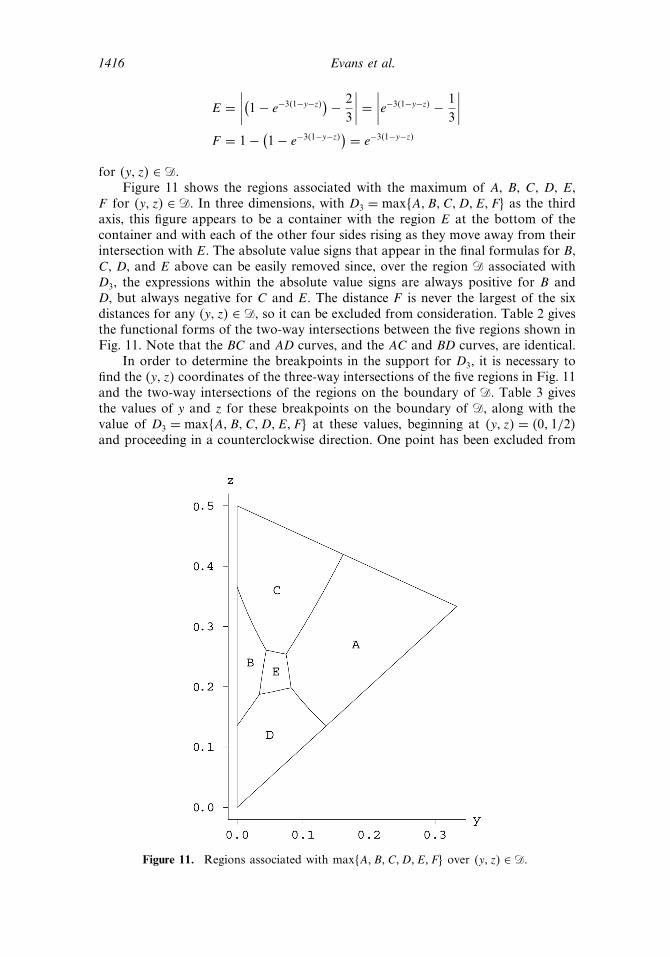
for �y� z� ∈ �.Figure 11 shows the regions associated with the maximum of A, B, C, D, E,

F for �y� z� ∈ �. In three dimensions, with D3 = max�A� B�C�D�E� F� as the thirdaxis, this figure appears to be a container with the region E at the bottom of thecontainer and with each of the other four sides rising as they move away from theirintersection with E. The absolute value signs that appear in the final formulas for B,C, D, and E above can be easily removed since, over the region � associated withD3, the expressions within the absolute value signs are always positive for B andD, but always negative for C and E. The distance F is never the largest of the sixdistances for any �y� z� ∈ �, so it can be excluded from consideration. Table 2 givesthe functional forms of the two-way intersections between the five regions shown inFig. 11. Note that the BC and AD curves, and the AC and BD curves, are identical.

In order to determine the breakpoints in the support for D3, it is necessary tofind the �y� z� coordinates of the three-way intersections of the five regions in Fig. 11and the two-way intersections of the regions on the boundary of �. Table 3 givesthe values of y and z for these breakpoints on the boundary of �, along with thevalue of D3 = max�A� B�C�D�E� F� at these values, beginning at �y� z� = �0� 1/2�and proceeding in a counterclockwise direction. One point has been excluded from

Figure 11. Regions associated with max�A� B�C�D�E� F� over �y� z� ∈ �.


Table 2Intersections of regions A, B, C, D, and E in �

AD z = − 13 ln

(43 − e−3y

)BD z = − 1

3 ln(e−3y − 1

3

)BC z = − 1

3 ln(43 − e−3y

)AC z = − 1

3 ln(e−3y − 1

3

)AE z = 1

3 ln[e3�1−y�

(e−3y − 2

3

)]DE z = 1

3 ln[13e

3�1−y�(1−√

1− 9e−3�1−y�)]

BE z = 13 ln

[e3�1−y�

(1− e−3y

)]CE z = 1

3 ln[16e

3�1−y�(− 1+√

1+ 36e−3�1−y�)]

Table 3 because of the intractability of the values �y� z�. The three-way intersectionbetween regions A, C, and the line z = �1− y�/2 can only be expressed in terms ofthe solution to a cubic equation. After some algebra, the point of intersection is thedecimal approximation �y� z� � �0�1608� 0�4196� and the associated value of D3 is2/3 minus the only real solution to the cubic equation

3d3 + d2 − 3e−3 = 0�

which yields

dAC = 79− 1

18�2916e−3 − 8+ c�1/3 − 2

9�2916e−3 − 8+ c�−1/3 � 0�3827�

where c = 108√729e−6 − 4e−3.

The three-way intersection points in the interior of � are more difficult todetermine than those on the boundary. The value of D3 associated with each of thesefour points is the single real root of a cubic equation on the support of D3. Theseequations and approximate solution values, in ascending order, are given in Table 4.For example, consider the value of the maximum at the intersection of regions A,

Table 3Intersection points along the boundary of �

y z D3

0 1/2 2/3− e−3/2 � 0�44350 ln�3�/3 1/3 � 0�33330 ln�3/2�/3 1/3 � 0�33330 0 2/3 � 0�6667ln�3/2�/3 ln�3/2�/3 1/3 � 0�33331/3 1/2 1− 1/e � 0�6321

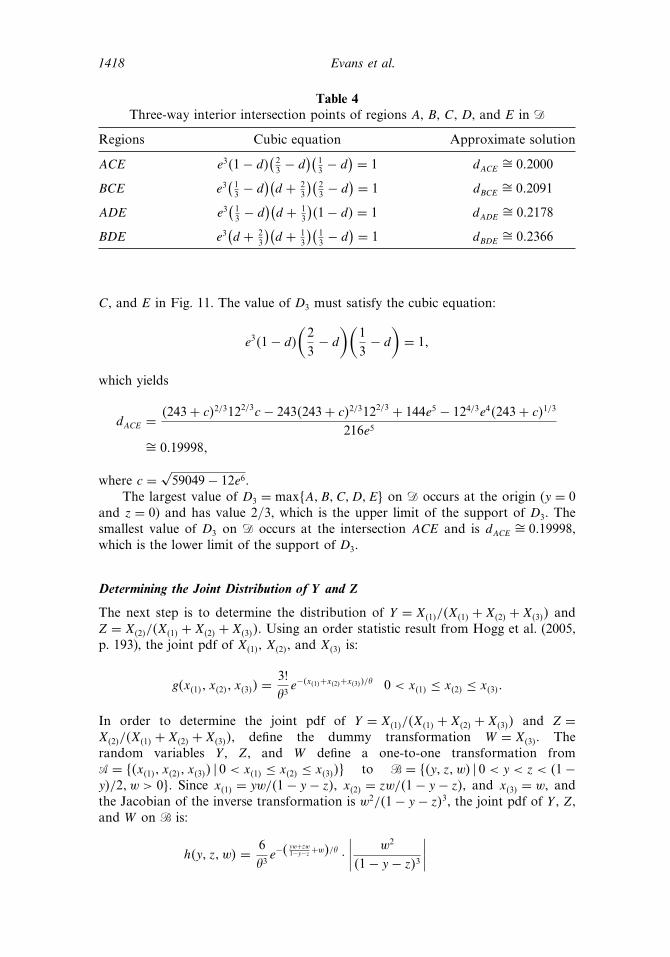
1418 Evans et al.

Table 4Three-way interior intersection points of regions A, B, C, D, and E in �

Regions Cubic equation Approximate solution

ACE e3�1− d�(23 − d

)(13 − d

) = 1 dACE � 0�2000

BCE e3(13 − d

)(d + 2

3

)(23 − d

) = 1 dBCE � 0�2091

ADE e3(13 − d

)(d + 1

3

)�1− d� = 1 dADE � 0�2178

BDE e3(d + 2

3

)(d + 1

3

)(13 − d

) = 1 dBDE � 0�2366

C, and E in Fig. 11. The value of D3 must satisfy the cubic equation:

e3�1− d�

(23− d

)(13− d

)= 1�

which yields

dACE = �243+ c�2/3122/3c − 243�243+ c�2/3122/3 + 144e5 − 124/3e4�243+ c�1/3

216e5

� 0�19998�

where c = √59049− 12e6.

The largest value of D3 = max�A� B�C�D�E� on � occurs at the origin (y = 0and z = 0) and has value 2/3, which is the upper limit of the support of D3. Thesmallest value of D3 on � occurs at the intersection ACE and is dACE � 0�19998,which is the lower limit of the support of D3.

Determining the Joint Distribution of Y and Z

The next step is to determine the distribution of Y = X�1�/�X�1� + X�2� + X�3�� andZ = X�2�/�X�1� + X�2� + X�3��. Using an order statistic result from Hogg et al. (2005,p. 193), the joint pdf of X�1�, X�2�, and X�3� is:

g�x�1�� x�2�� x�3�� =3!�3

e−�x�1�+x�2�+x�3��/� 0 < x�1� ≤ x�2� ≤ x�3��

In order to determine the joint pdf of Y = X�1�/�X�1� + X�2� + X�3�� and Z =X�2�/�X�1� + X�2� + X�3��, define the dummy transformation W = X�3�. Therandom variables Y , Z, and W define a one-to-one transformation from� = ��x�1�� x�2�� x�3�� 0 < x�1� ≤ x�2� ≤ x�3�� to � = ��y� z� w� � 0 < y < z < �1−y�/2� w > 0�. Since x�1� = yw/�1− y − z�, x�2� = zw/�1− y − z�, and x�3� = w, andthe Jacobian of the inverse transformation is w2/�1− y − z�3, the joint pdf of Y , Z,and W on � is:

h�y� z� w� = 6�3

e−�yw+zw1−y−z +w�/� ·

∣∣∣∣ w2

�1− y − z�3

∣∣∣∣


= 6�3

· w2

�1− y − z�3· e− w

�1−y−z�� y� z� w� ∈ ��

Integrating by parts, the joint density of Y and Z on � is:

fY�Z�y� z� =6

�3�1− y − z�3

∫ �

0w2e−

w�1−y−z�� dw = 12 �y� z� w� ∈ ��

i.e., Y and Z are uniformly distributed on �.

Determining the Distribution of D3

The cdf of D3 will be defined in a piecewise manner, with breakpoints at thefollowing ordered quantities: dACE , dBCE , dADE , dBDE , 1/3, dAC ,

23 − e−3/2, 1− 1

e, and

2/3. The cdf FD3�d� = Pr�D3 ≤ d� is found by integrating the joint pdf of Y and Z

over the appropriate limits, yielding:

FD3�d� =

0 d ≤ dACE

23

[ln(e3�1− d�

[23− d

] [13− d

])]2

dACE < d ≤ dBCE

23ln

[e6�1− d�

(23− d

)2 (23+ d

)(13− d

)2]ln(

1− d

2/3+ d

)dBCE < d ≤ dADE

43ln(d + 1/32/3− d

)ln(d + 2/31− d

)− 2

3

[ln(e3

[d + 2

3

] [d + 1

3

] [13− d

])]2

dADE < d ≤ dBDE

43ln(d + 1/32/3− d

)ln(d + 2/31− d

)dBDE < d ≤ 1

3

43ln(2/3− d

d + 1/3

)ln�1− d�− 2

3

[ln(d + 1/31− d

)]2 13< d ≤ dAC

1− 23

[ln(d + 1

3

)]2

− �1+ ln �1− d��2 − 3[1+ 2

3ln(23− d

)]2

dAC < d ≤ 23− e−3/2

1− 23

[ln(d + 1

3

)]2

− �1+ ln �1− d��223− e−3/2 < d ≤ 1− e−1

1− 23

[ln(d + 1

3

)]2

1− e−1 < d ≤ 23

1 d >23�

which is plotted in Fig. 12. Dots have been plotted at the breakpoints, with eachof the lower four tightly-clustered breakpoints from Table 4 corresponding to

1420 Evans et al.

Figure 12. The cdf of D3.

a horizontal plane intersecting one of the four corners of region E in Fig. 11.Percentiles of this distribution match the tabled values from Durbin (1975). We werenot able to establish a pattern between the cdf of D2 and the cdf of D3 that mightlead to a general expression for any n.

APPL was again used to calculate moments of D3. The decimal approximationsfor the mean, variance, skewness, and kurtosis, are, respectively, E�D3� � 0�3727,V�D3� � 0�008804, �3 � 0�4541, and �4 � 2�6538. These values were confirmed byMonte Carlo simulation. Although the functional form of the eight-segment PDF ofD3 is too lengthy to display here, it is plotted in Fig. 13, with the only non obviousbreakpoint being on the initial nearly-vertical segment at �dBCE� fD3

�dBCE�� 0�2091� 1�5624�.

Figure 13. The pdf of D3.


Acknowledgments

The first author acknowledges summer support from Rose–Hulman Institute ofTechnology. The second and third authors acknowledge FRA support from theCollege of William & Mary. The authors also acknowledge the assistance of BillGriffith, Thom Huber, and David Kelton in selecting data sets for the case studies.

References

Cho, S. K., Spiegelberg-Planer, R. (2002). Country nuclear power profiles. http://www-pub.iaea.org/MTCD/publications/PDF/cnpp2003/CNPP_Webpage/PDF/2002/index.htmAccessed August 1, 2004.

D’Agostino, H., Stephens, M. (1986). Goodness-of-Fit Techniques. New York: MarcelDekker.

Drew, J. H., Glen, A. G., Leemis, L. M. (2000). Computing the cumulative distributionfunction of the Kolmogorov–Smirnov statistic. Computational Statistics and Data Analysis34:1–15.

Durbin, J. (1975). Kolmogorov–Smirnov tests when parameters are estimated withapplications to tests of exponentiality and tests on spacings. Biometrika 62:5–22.

Glen, A. G., Evans, D. L., Leemis, L. M. (2001). APPL: a probability programminglanguage. The American Statistician 55:156–166.

Hogg, R. V., McKean, J. W., Craig, A. T. (2005). Mathematical Statistics. 6th ed. UpperSaddle River, NJ: Prentice–Hall.

Law, A. M., Kelton, W. D. (2000). Simulation Modeling and Analysis. 3rd ed. New York:McGraw-Hill.

Lawless, J. F. (2003). Statistical Models and Methods for Lifetime Data. 2nd ed. New York:John Wiley & Sons.

Lehmann, E. L. (1959). Testing Statistical Hypotheses. New York: John Wiley & Sons.Lilliefors, H. (1969). On the Kolmogorov–Smirnov test for the exponential distribution with

mean unknown. Journal of the American Statistical Association 64:387–389.Marsaglia, G., Tsang, W. W., Wang, J. (2003). Evaluating Kolmogorov’s distribution.

Journal of Statistical Software 8:18. URL: http://www.jstatsoft.org/v08/i18/Rigdon, S., Basu, A. P. (2000). Statistical Methods for the Reliability of Repairable Systems.

New York: John Wiley & Sons.Stephens, M. A. (1974). EDF statistics for goodness of fit and some comparisons. Journal of

the American Statistical Association 69:730–737.

goodness-of-fittest …leemis/2008commst.pdfd n=maxd +d − although the test statistic d n is easy...

Documents