government spending and its financing - unical · government outlays, the total spending by the...
TRANSCRIPT

580
Chapter 15Government Spending and Its Financing
At every level of government, from the town hall to the White House, fiscal policy—government decisions about how much to spend, what to spend for, and how to finance its spending—is of central importance. Politicians and the public understand that the government’s fiscal choices have a direct impact on the “bread and butter” issues of how much they pay in taxes and what govern-ment benefits and services they receive. Equally important are the effects of fiscal policy on the economy. In recent years, people have become more aware of the macroeconomic effects of fiscal policy as the economic implications of govern-ment budget deficits and surpluses, tax reform, Social Security reform, govern-ment bailouts, and other aspects of fiscal policy have been extensively debated.
In this chapter we take a close look at fiscal policy and its macroeconomic effects. To provide some background, we begin with definitions and facts about the government’s budget. We then discuss some basic fiscal policy issues, includ-ing the effects of government spending and taxes on economic activity, the bur-den of government debt, and the link between budget deficits and inflation.
Before getting into the analytical issues of fiscal policy, we set the stage by looking at the components of the government budget and their recent trends. We discuss three main aspects of the budget: (1) spending, or outlays; (2) tax revenues, or receipts; and (3) the budget surplus or deficit. Our discussion reviews and builds on Chapter 2, in which we introduced basic budget concepts.
Government OutlaysGovernment outlays, the total spending by the government during a period of time, are classified into three primary categories: government purchases, transfer payments, and net interest payments.
1. Government purchases (G) are government expenditures on currently produced goods and services, including capital goods. Government spending on capital goods, or government investment, accounts for about one-sixth of government purchases of goods and services. The remaining five-sixths of government purchases are government consumption expenditures.
2. Transfer payments (TR) are payments made to individuals for which the gov-ernment does not receive current goods or services in exchange. Examples of
15.1 The Government Budget: Some Facts and FiguresUse the measures of government outlays and taxes to measure government surpluses and deficits.
Learning Objectives
15.1 Use the measures of government outlays and taxes to measure government surpluses and deficits.
15.2 Describe how government spending and taxing decisions affect the macroeconomy.
15.3 Discuss the economic effects of government deficits and debt.
15.4 Explain the link between deficits and inflation.
ChapTer 15 | Government Spending and Its Financing 581
transfers are Social Security benefit payments, military and civil service pen-sions, unemployment insurance, welfare payments (Temporary Assistance for Needy Families), and Medicare.1
3. Net interest payments (INT) are the interest paid to the holders of government bonds less the interest received by the government—for example, on out-standing government loans to students or farmers.
In addition there is a minor category called subsidies less surpluses of govern-ment enterprises. Subsidies are government payments that are intended to affect the production or prices of various goods. Examples are price support payments to farmers and fare subsidies for mass transit systems. The surpluses of govern-ment enterprises represent the profits of government-run enterprises such as the Tennessee Valley Authority (an electricity producer). This category of outlays is relatively small, so for simplicity we will ignore it.
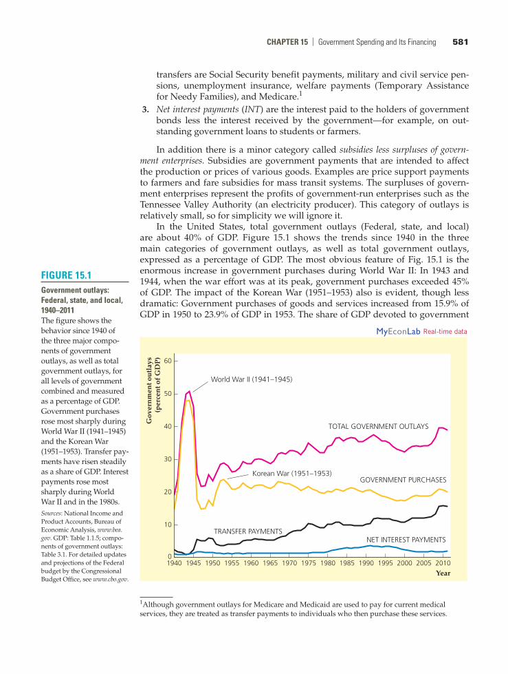
In the United States, total government outlays (Federal, state, and local) are about 40% of GDP. Figure 15.1 shows the trends since 1940 in the three main categories of government outlays, as well as total government outlays, expressed as a percentage of GDP. The most obvious feature of Fig. 15.1 is the enormous increase in government purchases during World War II: In 1943 and 1944, when the war effort was at its peak, government purchases exceeded 45% of GDP. The impact of the Korean War (1951–1953) also is evident, though less dramatic: Government purchases of goods and services increased from 15.9% of GDP in 1950 to 23.9% of GDP in 1953. The share of GDP devoted to government
1Although government outlays for Medicare and Medicaid are used to pay for current medical services, they are treated as transfer payments to individuals who then purchase these services.
FiGure 15.1Government outlays: Federal, state, and local, 1940–2011The figure shows the behavior since 1940 of the three major compo-nents of government outlays, as well as total government outlays, for all levels of government combined and measured as a percentage of GDP. Government purchases rose most sharply during World War II (1941–1945) and the Korean War (1951–1953). Transfer pay-ments have risen steadily as a share of GDP. Interest payments rose most sharply during World War II and in the 1980s.Sources: National Income and Product Accounts, Bureau of Economic Analysis, www.bea. gov. GDP: Table 1.1.5; compo-nents of government outlays: Table 3.1. For detailed updates and projections of the Federal budget by the Congressional Budget Office, see www.cbo.gov.
0
10
20
30
40
50
60
1940 1945 1950 1955 1960 1965 1970 1975 1980 1985 1990 1995 2000 2005 2010
Gov
ern
men
t ou
tlay
s(p
erce
nt o
f G
DP
)
Year
TOTAL GOVERNMENT OUTLAYS
GOVERNMENT PURCHASES
TRANSFER PAYMENTSNET INTEREST PAYMENTS
World War II (1941–1945)
Korean War (1951–1953)
MyEconLab Real-time data

582 parT 4 | Macroeconomic Policy: Its Environment and Institutions
purchases drifted gradually downward from about 23% of GDP in the late 1960s to around 17% of GDP in the late 1990s, but has since risen to about 20% of GDP.
Figure 15.1 also shows that transfer payments rose steadily as a share of GDP from the early 1950s until the early 1980s, doubling their share of GDP during that thirty-year period. Transfers averaged about 12% of GDP in the 2000s before the financial crisis in 2008, and have since averaged about 16%. The long-term increase in transfer payments is the result of the creation of new social programs (such as Medicare and Medicaid in 1965), the expansion of benefits under exist-ing programs (such as Social Security, which is discussed later in the chapter in the Application “Social Security: How Can It Be Fixed?” pp. 597–599), and the increased number of people covered by the various programs.
Finally, Fig. 15.1 shows how net interest payments—interest payments, for short—have evolved. Because interest payments are much smaller than the other two categories of government outlays, they appear to fluctuate less. However, interest payments rose sharply as a percentage of GDP in two periods. First, inter-est payments nearly doubled from 0.95% of GDP in 1941 to 1.85% of GDP in 1946, reflecting the large amount of government borrowing done to finance the war effort during World War II. Second, interest payments as a share of GDP doubled during the 1980s, rising from 1.6% in 1979 to 3.3% in 1989. This increase reflected both increased borrowing by the government and the generally high level of in-terest rates during the 1980s. Net interest payments as a share of GDP declined in the 1990s, as interest rates fell and the government budget moved into surplus and fell further in the 2000s as interest rates declined even more.
How does the rate of government expenditure in the United States compare with rates in other countries with similar living standards? Because official account-ing rules for measuring the government budget vary widely among countries, the answer isn’t as straightforward as you might think. Nevertheless, Table 15.1 compares the ratios of government spending to GDP for eighteen countries in the
TaBLe 15.1Government Spending in eighteen OeCD Countries, percentage of GDp, 2011
Country
United States 41.7Japan 42.8Germany 45.7France 56.1Italy 49.9United Kingdom 49.1Canada 42.9Australia 35.2Austria 50.5Belgium 53.4Denmark 57.9Finland 54.1Greece 50.1Iceland 46.1Ireland 48.7Netherlands 50.1Spain 43.6Sweden 51.3Source: OECD Economic Outlook, Annex Table 25, www.oecd.org/eco/economicoutlook.htm.
ChapTer 15 | Government Spending and Its Financing 583
Organization for Economic Cooperation and Development (OECD). The United States has the second lowest rate of total government spending, as a percentage of GDP; the lowest is Australia at just 35.2%. The low rate of government spending in the United States relative to most of the other countries largely reflects the more extensive government-financed social welfare programs (such as national health insurance) in those countries.
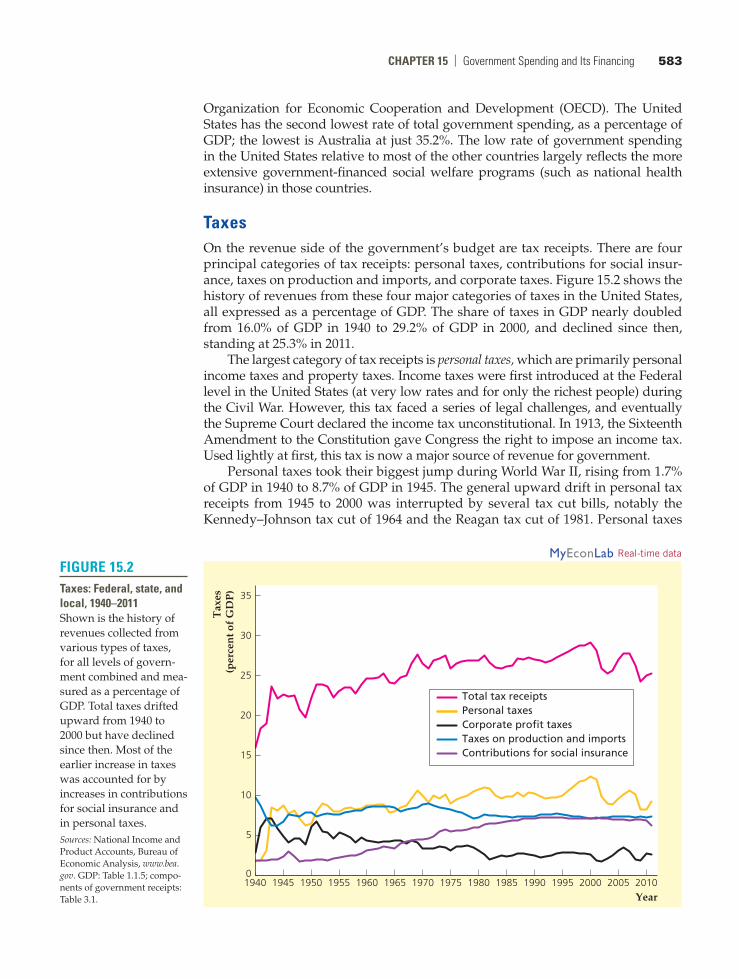
TaxesOn the revenue side of the government’s budget are tax receipts. There are four principal categories of tax receipts: personal taxes, contributions for social insur-ance, taxes on production and imports, and corporate taxes. Figure 15.2 shows the history of revenues from these four major categories of taxes in the United States, all expressed as a percentage of GDP. The share of taxes in GDP nearly doubled from 16.0% of GDP in 1940 to 29.2% of GDP in 2000, and declined since then, standing at 25.3% in 2011.
The largest category of tax receipts is personal taxes, which are primarily personal income taxes and property taxes. Income taxes were first introduced at the Federal level in the United States (at very low rates and for only the richest people) during the Civil War. However, this tax faced a series of legal challenges, and eventually the Supreme Court declared the income tax unconstitutional. In 1913, the Sixteenth Amendment to the Constitution gave Congress the right to impose an income tax. Used lightly at first, this tax is now a major source of revenue for government.
Personal taxes took their biggest jump during World War II, rising from 1.7% of GDP in 1940 to 8.7% of GDP in 1945. The general upward drift in personal tax receipts from 1945 to 2000 was interrupted by several tax cut bills, notably the Kennedy–Johnson tax cut of 1964 and the Reagan tax cut of 1981. Personal taxes
FiGure 15.2Taxes: Federal, state, and local, 1940–2011Shown is the history of revenues collected from various types of taxes, for all levels of govern-ment combined and mea-sured as a percentage of GDP. Total taxes drifted upward from 1940 to 2000 but have declined since then. Most of the earlier increase in taxes was accounted for by increases in contributions for social insurance and in personal taxes.Sources: National Income and Product Accounts, Bureau of Economic Analysis, www.bea. gov. GDP: Table 1.1.5; compo-nents of government receipts: Table 3.1.
0
5
10
15
20
25
30
35
1940 1945 1950 1955 1960 1965 1970 1975 1980 1985 1990 1995 2000 2005 2010
Tax
es(p
erce
nt o
f G
DP
)
Year
Total tax receiptsPersonal taxesCorporate profit taxesTaxes on production and importsContributions for social insurance
MyEconLab Real-time data
584 parT 4 | Macroeconomic Policy: Its Environment and Institutions
rose as a result of the deficit-reduction efforts of President Clinton, then declined with President Bush’s tax cuts in the 2000s.
Figure 15.2 shows that a large share of the increase in tax receipts since World War II reflects the increase in a second category of taxes, contributions for social insurance (primarily Social Security taxes). Social insurance contributions usually are levied as a fixed percentage of a worker’s salary, up to a ceiling; income above that ceiling isn’t taxed.2 In most cases the worker’s contributions are matched by the employer so that the deduction appearing on the worker’s paycheck reflects only half the total tax levied. Increases in social insurance contributions are the result of increases both in the contribution rate and higher ceilings on the amount of income subject to the tax.
A third category of tax receipts is taxes on production and imports, mainly sales taxes. These taxes declined as a share of GDP during World War II and haven’t shown any significant long-term increase or decrease since.
A final category of tax receipts is corporate taxes, particularly corporate profit taxes. Figure 15.2 shows that corporate taxes rose sharply during World War II and the Korean War, then drifted gradually downward as a share of GDP from the mid 1950s until the mid 1980s. Corporate tax receipts have accounted for 2% to 3% of GDP in recent years.
The Composition of Outlays and Taxes: The Federal Government Versus State and Local Governments. The components of government spending shown in Fig. 15.1 and the components of taxes shown in Fig. 15.2 lump together Federal, state, and local governments. For most purposes of macroeconomic anal-ysis, combining Federal, state, and local fiscal policy is the most sensible choice. The macroeconomic effect of a new highway-building program, for example, shouldn’t depend on whether the new highways are financed from the Federal, state, or local budgets—or from a combination of those budgets. In this respect the tendency of many news stories about fiscal policy to focus exclusively on the Federal government’s budget can be misleading.
Nevertheless, it is useful to know that in the United States, Federal govern-ment budgets have a much different composition, on both the expenditure and the revenue sides, than those of state and local governments. A summary of the major components of both the Federal and the combined state and local government budgets for 2011 is given in Table 15.2. Note in particular the following points:
1. Government consumption expenditures. About two-thirds of state and local current expenditures (expenditures excluding investment) is for goods and services. In contrast, about 30% of Federal current expenditures is for goods and services, and about two-thirds of this amount is for national defense. More than 80% of government consumption expenditures on nondefense goods and services in the United States comes from state and local governments.
2. Transfer payments. The Federal budget is more heavily weighted toward transfer payments (particularly, benefits from Social Security and related pro-grams) than state and local budgets are.
3. Grants in aid. Grants in aid are payments made by the Federal govern-ment to state and local governments to help support various education,
2Note that there is no ceiling for Medicare taxes.

ChapTer 15 | Government Spending and Its Financing 585
transportation, and welfare programs. Grants in aid appear as a current expenditure for the Federal government and as a receipt for state and local governments. In 2011, these grants made up more than one-fourth of state and local government receipts.
4. Net interest paid. Because of the large quantity of Federal government bonds outstanding, net interest payments are an important component of Federal spending. In contrast, net interest payments for state and local governments are usually small and sometimes negative, which occurs when state and local governments (which hold substantial amounts of Federal government bonds) receive more interest than they pay out.
5. Composition of taxes. More than 80% of Federal government receipts come from personal taxes (primarily the Federal income tax) and contributions for social insurance. Less than 15% of Federal revenues are from corporate taxes, and less than 5% are from taxes on production and imports such as sales taxes. In contrast, taxes on production and imports account for about half
TaBLe 15.2Government receipts and Current expenditures, 2011
Federal State and local
Current expendituresBillions
of dollars
Percentage of current
expendituresBillions of
dollars
Percentage of current
expenditures
Consumption expenditures 1072.1 29.5 1475.2 68.6 National defense 716.9 19.7 0.0 0.0 Nondefense 355.2 9.8 1475.2 68.6Transfer payments 1813.3 49.9 558.0 26.0Grants in aid 492.5 13.6 0.0 0.0Net interest paid 282.1 7.8 116.0 5.4Net other expenditures* −25.5 −0.7 0.5 0.0Total current expenditures 3634.5 100.0 2149.7 100.0
Federal State and local
ReceiptsBillions
of dollarsPercentage of receipts
Billions of dollars
Percentage of receipts
Personal taxes 1072.0 44.1 325.7 17.3Contributions for social insurance 907.3 37.4 21.6 1.1Taxes on production and imports 110.8 4.6 987.1 52.6Corporate taxes 338.2 13.9 51.5 2.7Grants in aid 0.0 0.0 492.5 26.2Total receipts 2428.3 100.0 1878.4 100.0
Current deficit (current expenditures less receipts; negative if surplus)
1206.2 271.3
Primary current deficit (negative if surplus)
924.1 155.3
*Subsidies less surpluses of government enterprises, taxes from the rest of the world, dividends, rents and royalties, and transfer receipts.
Note: Components may not add exactly to totals owing to rounding.Source: BEA Web site, www.bea.gov, Tables 3.2, 3.3, and 3.9.5.

586 parT 4 | Macroeconomic Policy: Its Environment and Institutions
of state and local revenues. About one-fifth of state and local revenues come from personal taxes (both income taxes and property taxes) and contributions for social insurance. As already mentioned, state and local governments also count as revenue the grants in aid they receive from the Federal government.
Deficits and SurplusesGovernment outlays need not equal tax revenues in each period. In Chapter 2 we showed that, when government outlays exceed revenues, there is a government budget deficit (or simply a deficit); when revenues exceed outlays, there is a govern-ment budget surplus. For ease of reference we write the definition of the deficit as
deficit = outlays - tax revenues (15.1) = (government purchases + transfers + net interest) - tax revenues = (G + TR + INT) - T.
A second deficit concept, called the primary government budget deficit, excludes net interest from government outlays:
primary deficit = outlays - net interest - tax revenues (15.2)
= (government purchases + transfers) - tax revenues = (G + TR) - T.The primary deficit is the amount by which government purchases and transfers exceed tax revenues; the primary deficit plus net interest payments equals the deficit. Figure 15.3 illustrates the relationship between the two concepts.
FiGure 15.3The relationship between the total budget deficit and the primary deficitThe standard measure of the total govern-ment budget deficit is the amount by which government outlays exceed tax revenues. The primary deficit is the amount by which government purchases plus transfers exceed tax revenues. The total budget deficit equals the primary deficit plus net interest payments.
OUTLAYS
DEFICIT
REVENUES
Tax revenues
Government purchasesand
transfers
Primary deficit
Net interestNet interest
ChapTer 15 | Government Spending and Its Financing 587
Why have two deficit concepts? The reason is that each answers a different question. The standard or total budget deficit answers the question: How much does the government currently have to borrow to pay for its to-tal outlays? When measured in nominal terms, the deficit during any year is the number of additional dollars that the government must borrow during that year.
The primary deficit answers the question: Can the government afford its current programs? If the primary deficit is zero, the government is collecting just enough tax revenue to pay for its current purchases of goods and services and its current social programs (as reflected by transfer payments). If the primary deficit is greater than zero, current government purchases and social programs cost more than current tax revenue can pay for. Net interest payments are ignored in the primary deficit because they represent not current program costs but costs of past expenditures financed by government borrowing.
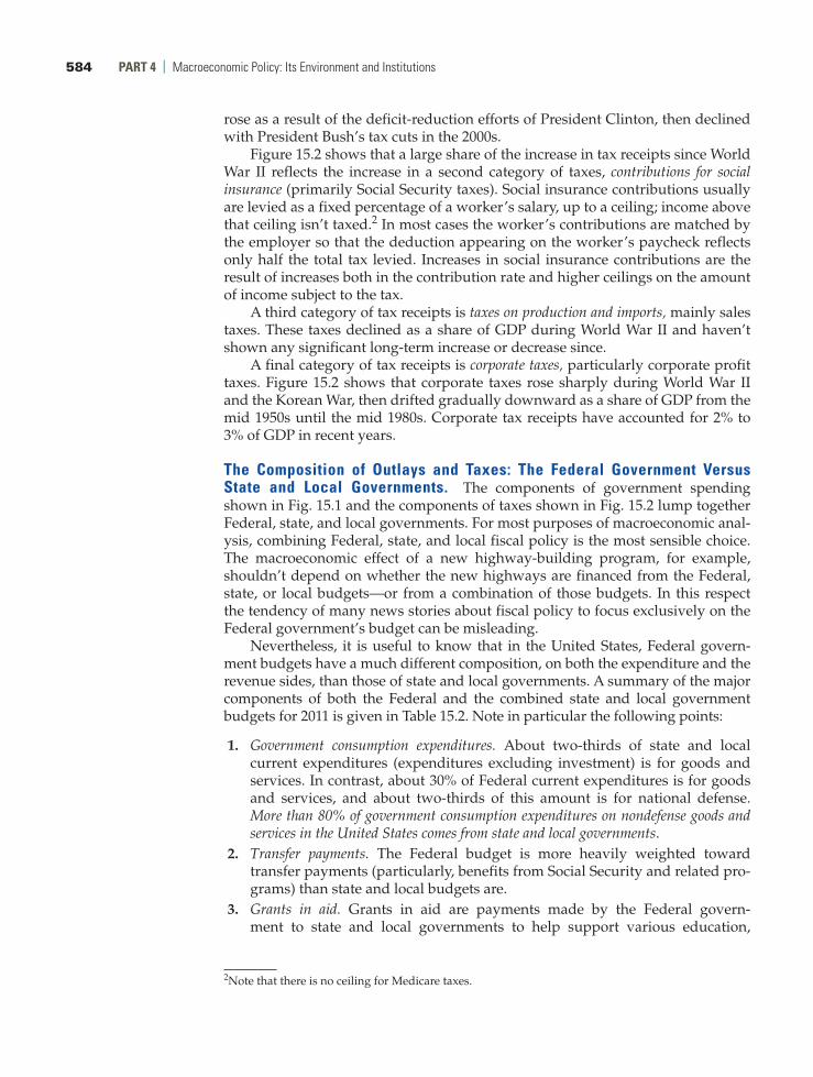
The separation of government purchases into government investment and government consumption expenditures introduces another set of deficit concepts: the current deficit and the primary current deficit. The current deficit is equivalent to the deficit in Eq. (15.1), with outlays replaced by current expenditures, which are all government outlays except government investment. The primary current deficit is the current deficit minus interest payments. Table 15.2 shows the current deficit and the primary current deficit for 2011.
Figure 15.4 shows the current deficit and primary current deficit for all levels of government combined as a percentage of GDP since 1940. Again, the World War II period stands out; the government financed only part of the war
FiGure 15.4Current deficit and primary current deficit: Federal, state, and local, 1940–2011Shown are the current government budget deficit and the primary current deficit, both mea-sured as a percentage of GDP, since 1940. The government ran large primary current deficits during World War II and after the financial crisis in 2008. The widening gap between the current deficit and the current primary deficit between 1975 and 1991 reflects increasing interest pay-ments on the govern-ment’s accumulated debt.Sources: National Income and Product Accounts, Bureau of Economic Analysis, www.bea. gov. GDP: Table 1.1.5; current deficit: Table 3.1; primary cur-rent deficit: authors’ calcula-tions from data on deficit and net interest paid in Table 3.1.
–6
–4
–2
0
2
4
6
8
10
12
14
1940 1945 1950 1955 1960 1965 1970 1975 1980 1985 1990 1995 2000 2005 2010
Def
icit
s(p
erce
nt o
f G
DP
)
Year
World War II (1941–1945)
CURRENTDEFICIT
PRIMARYCURRENTDEFICIT
MyEconLab Real-time data
588 parT 4 | Macroeconomic Policy: Its Environment and Institutions
effort with taxes and thus ran large primary and overall deficits.3 Large defi-cits ( using both concepts) also occurred in the mid 1970s and again in the early 1980s. Although the primary deficit actually became a primary surplus for sev-eral years in the 1980s and 1990s, large interest payments kept the overall deficit large until the late 1990s, when the overall budget went into surplus. Tax cuts in the early 2000s eliminated the large primary current surplus of the late 1990s. The Federal government increased spending during the Great Recession from 2007 to 2009, leading to large current deficits and primary current deficits for several years.
How does fiscal policy affect the performance of the macroeconomy? Economists emphasize three main ways by which government spending and taxing decisions influence macroeconomic variables such as output, employment, and prices: (1) aggregate demand, (2) government capital formation, and (3) incentives.
Fiscal policy and aggregate DemandFiscal policy can affect economic activity by influencing the total amount of spending in the economy, or aggregate demand. Recall that aggregate demand is represented by the intersection of the IS and LM curves. In either the classical or the Keynesian IS–LM model, a temporary increase in government purchases re-duces desired national saving and shifts the IS curve up and to the right, thereby raising aggregate demand.
Classical and Keynesian economists have different beliefs about the effect of tax changes on aggregate demand. Classicals usually accept the Ricardian equivalence proposition, which says that lump-sum tax changes do not affect desired national saving and thus have no impact on the IS curve or aggregate demand.4 Keynesians generally disagree with this conclusion; in the Keynesian view, a cut (for example) in taxes is likely to stimulate desired consumption and reduce desired national sav-ing, thereby shifting the IS curve up and to the right and raising aggregate demand.
Classicals and Keynesians also disagree over the question of whether fiscal policy should be used to fight the business cycle. Classicals generally reject at-tempts to smooth business cycles, by fiscal policy or by other means. In contrast, Keynesians argue that using fiscal policy to stabilize the economy and maintain full employment—for example, by cutting taxes and raising spending when the economy is in a recession—is desirable.
However, even Keynesians admit that the use of fiscal policy as a stabilization tool is difficult. A significant problem is lack of flexibility. The government’s bud-get has many purposes besides macroeconomic stabilization, such as maintaining national security, providing income support for eligible groups, developing the nation’s infrastructure (roads, bridges, and public buildings), and supplying govern-ment services (education and public health). Much of government spending is com-mitted years in advance (as in weapons development programs) or even decades in
15.2 Government Spending, Taxes, and the MacroeconomyDescribe how government spending and taxing decisions affect the macroeconomy.
4We introduced Ricardian equivalence in Chapter 4. We discuss this idea further in Section 15.3.
3Much of the increased government spending in World War II was on government investment, which is not counted in the current deficit. As a result, the overall deficit, defined in Eq. (15.1), was even higher than the current deficit and exceeded 20% of GDP, as you can see by comparing Fig. 15.1 with Fig. 15.2.

ChapTer 15 | Government Spending and Its Financing 589
advance (as for Social Security benefits). Expanding or contracting total government spending rapidly for macroeconomic stabilization purposes thus is difficult with-out either spending wastefully or compromising other fiscal policy goals. Taxes are somewhat easier to change than spending, but the tax laws also have many different goals and may be the result of a fragile political compromise that isn’t easily altered.
Compounding the problem of inflexibility is the problem of long time lags that result from the slow-moving political process by which fiscal policy is made. From the time a spending or tax proposal is made until it goes into effect is rarely less than eighteen months. This lag makes effective countercyclical use of fiscal policy difficult because (for example), by the time an antirecession fiscal measure actually had an impact on the economy, the recession might already be over.
automatic Stabilizers and the Full-employment Deficit. One way to get around the problems of fiscal policy inflexibility and long lags that impede the use of countercyclical fiscal policies is to build automatic stabilizers into the bud-get. Automatic stabilizers are provisions in the budget that cause government spending to rise or taxes to fall automatically—without legislative action—when GDP falls. Similarly, when GDP rises, automatic stabilizers cause spending to fall or taxes to rise without any need for direct legislative action.
A good example of an automatic stabilizer is unemployment insurance. When the economy goes into a recession and unemployment rises, more people receive unemployment benefits, which are paid automatically without further action by Congress. Thus the unemployment insurance component of transfers rises during recessions, making fiscal policy automatically more expansionary.5
Quantitatively, the most important automatic stabilizer is the income tax sys-tem. When the economy goes into a recession, people’s incomes fall, and they pay less income tax. This “automatic tax cut” helps cushion the drop in disposable income and (according to Keynesians) prevents aggregate demand from falling as far as it might otherwise. Likewise, when people’s incomes rise during a boom, the government collects more income tax revenue, which helps restrain the in-crease in aggregate demand. Keynesians argue that this automatic fiscal policy is a major reason for the increased stability of the economy since World War II.
A side effect of automatic stabilizers is that government budget deficits tend to increase in recessions because government spending automatically rises and taxes automatically fall when GDP declines. Similarly, the deficit tends to fall in booms. To distinguish changes in the deficit caused by recessions or booms from changes caused by other factors, some economists advocate the use of a deficit measure called the full-employment deficit. The full-employment deficit indicates what the government budget deficit would be—given the tax and spending policies currently in force—if the economy were operating at its full-employment level.6 Because it eliminates the effects of automatic stabilizers, the full-employment deficit measure is affected primarily by changes in fiscal policy reflected in new legislation. In particular, expan-sionary fiscal changes—such as increases in government spending programs or (in the Keynesian model) reduced tax rates—raise the full-employment budget deficit, whereas contractionary fiscal changes reduce the full-employment deficit.
5This statement is based on the Keynesian view that an increase in transfers—which is equivalent to a reduction in taxes—raises aggregate demand.6In practice, the calculation of full-employment deficits is based on the Keynesian assumption that recessions reflect deviations from full employment rather than the classical assumption that (in the absence of misperceptions) recessions reflect changes in full-employment output.

590 parT 4 | Macroeconomic Policy: Its Environment and Institutions
Figure 15.5 shows the actual and full-employment budget deficits (as per-centages of full-employment output) of the Federal government since 1962. Note that the actual budget deficit substantially exceeded the full-employment budget deficit during or slightly after the recessions of 1973–1975, 1981–1982, 1990–1991, 2001, and 2007–2009 when output was below its full-employment level. The dif-ference between the two deficit measures reflects the importance of automatic stabilizers in the budget.
Government Capital FormationThe health of the economy depends not only on how much the government spends but also on how it spends its resources. For example, as discussed in Chapter 6, the quantity and quality of public infrastructure—roads, schools, public hospitals, and the like—are potentially important for the rate of economic growth. Thus the formation of government capital—long-lived physical assets owned by the government—is one way that fiscal policy affects the macroeconomy. The govern-ment budget affects not only physical capital formation but also human capital formation. At least part of government expenditures on health, nutrition, and education are an investment, in the sense that they will lead to a more productive work force in the future.
The official figures for government capital investment focus on physical capital formation and exclude human capital formation. In 2011 Federal govern-ment investment expenditures were $160.8 billion (about one-eighth of Federal purchases of goods and services), with two-thirds of investment spending for national defense and one-third for nondefense government capital. State and local government investment was $322.5 billion (about one-fifth of state and local
FiGure 15.5Full-employment and actual budget deficits, 1962–2011The actual and full-employment Federal budget deficits are shown as a percentage of full-employment out-put. The actual budget deficit exceeded the full-employment deficit by substantial amounts dur-ing or slightly after the 1973–1975, 1981–1982, 1990–1991, 2001, and 2007–2009 recessions, reflecting the importance of automatic stabilizers.Source: Congressional Budget Office Web site at www.cbo.gov/publication/42907.
–4
–2
0
2
4
6
8
10
12
1960 1965 1970 1975 1980 1985 1990 1995 2000 2005 2010
Def
icit
s(p
erce
nt o
f fu
ll-e
mp
loym
ent G
DP
)
Year
ACTUALDEFICIT
FULL-EMPLOYMENTDEFICIT

ChapTer 15 | Government Spending and Its Financing 591
government purchases of goods and services). The composition of government investment by state and local governments differs from that by the Federal gov-ernment. Most Federal government investment is in the form of equipment (such as military hardware and software) rather than structures, but about four-fifths of state and local government investment is for structures.
incentive effects of Fiscal policyThe third way in which fiscal policy affects the macroeconomy is by its effects on incentives. Tax policies in particular can affect economic behavior by changing the financial rewards to various activities. For example, in Chapter 4 we showed how tax rates influence the incentives of households to save and of firms to make capital investments.
average Versus Marginal Tax rates. To analyze the effects of taxes on eco-nomic incentives, we need to distinguish between average and marginal tax rates. The average tax rate is the total amount of taxes paid by a person (or a firm), divided by the person’s before-tax income. The marginal tax rate is the fraction of an additional dollar of income that must be paid in taxes. For example, suppose that in a particular country no taxes are levied on the first $10,000 of income and that a 25% tax is levied on all income above $10,000 (see Table 15.3). Under this in-come tax system a person with an income of $18,000 pays a tax of $2000. Thus her average tax rate is 11.1% ($2000 in taxes divided by $18,000 in before-tax income). However, this taxpayer’s marginal tax rate is 25%, because a $1.00 increase in her income will increase her taxes by $0.25. Table 15.3 shows that everyone with an income higher than $10,000 faces the same marginal tax rate of 25% but that the average tax rate increases with income.
We can show why the distinction between average and marginal tax rates is important by considering the individual’s decision about how much labor to sup-ply. The effects of a tax increase on the amount of labor supplied depend strongly on whether average or marginal taxes are being increased. Economic theory predicts that an increase in the average tax rate, with the marginal tax rate held constant, will increase the amount of labor supplied at any (before-tax) real wage. In contrast, the theory predicts that an increase in the marginal tax rate, with the average tax rate held constant, will decrease the amount of labor supplied at any real wage.
To explain these conclusions, let’s first consider the effects of a change in the average tax rate. Returning to our example from Table 15.3, imagine that the mar-ginal tax rate stays at 25% but that now all income over $8000 (rather than all in-come over $10,000) is subject to a 25% tax. The taxpayer with an income of $18,000
TaBLe 15.3Marginal and average Tax rates: an example (Total Tax = 25% of income over $10,000)
Income Income–$10,000 TaxAverage tax rate
Marginal tax rate
$ 18,000 $ 8,000 $ 2,000 11.1% 25%50,000 40,000 10,000 20.0% 25%
100,000 90,000 22,500 22.5% 25%

592 parT 4 | Macroeconomic Policy: Its Environment and Institutions
finds that her tax bill has risen from $2000 to $2500, or 0.25(+18,000 - +8000), so her average tax rate has risen from 11.1% to 13.9%, or $2500/$18,000. As a re-sult, the taxpayer is $500 poorer. Because she is effectively less wealthy, she will increase the amount of labor she supplies at any real wage (see Summary table 4, p. 83). Hence an increase in the average tax rate, holding the marginal tax rate fixed, shifts the labor supply curve (in a diagram with the before-tax real wage on the vertical axis) to the right.7
Now consider the effects of an increase in the marginal tax rate, with the aver-age tax rate constant. Suppose that the marginal tax rate on income increases from 25% to 40% and the rise is accompanied by other changes in the tax law that keep the average tax rate—and thus the total amount of taxes paid by the typical tax-payer— the same. To be specific, suppose that the portion of income not subject to tax is increased from $10,000 to $13,000. Then for the taxpayer earning $18,000, total taxes are $2000, or 0.40($18,000 - $13,000), and the average tax rate of 11.1%, or $2000/$18,000, is the same as it was under the original tax law.8
With the average tax rate unchanged, the taxpayer’s wealth is unaffected, and so there is no change in labor supply stemming from a change in wealth. However, the increase in the marginal tax rate implies that the taxpayer’s after-tax reward for each extra hour worked declines. For example, if her wage is $20 per hour before taxes, at the original marginal tax rate of 25%, her actual take-home pay for each extra hour of work is $15 ($20 minus 25% of $20, or $5, in taxes). At the new marginal tax rate of 40%, the taxpayer’s take-home pay for each extra hour of work is only $12 ($20 in before-tax wages minus $8 in taxes). Because ex-tra hours of work no longer carry as much reward in terms of real income earned, at any specific before-tax real wage the taxpayer is likely to work fewer hours and enjoy more leisure instead. Thus, if the average tax rate is held fixed, an increase in the marginal tax rate causes the labor supply curve to shift to the left.9
Tax-induced Distortions and Tax rate Smoothing. Because taxes affect eco-nomic incentives, they change the pattern of economic behavior. If the invisible hand of free markets is working properly, the pattern of economic activity in the absence of taxes is the most efficient, so changes in behavior caused by taxes re-duce economic welfare. Tax-induced deviations from efficient, free-market out-comes are called distortions.
To illustrate the idea of a distortion, let’s go back to the example of the worker whose before-tax real wage is $20. Because profit-maximizing employers demand labor up to the point that the marginal product of labor equals the real wage, the real output produced by an extra hour of the worker’s labor (her marginal prod-uct) also is $20. Now suppose that the worker is willing to sacrifice leisure to work an extra hour if she receives at least $14 in additional real earnings. Because the value of what the worker can produce in an extra hour of labor exceeds the value that she places on an extra hour of leisure, her working the extra hour is economi-cally efficient.
7In terms of the analysis of Chapter 3, the increase in the average tax rate has a pure income effect on labor supply.8Although the average tax rate is unchanged for the taxpayer earning $18,000, the average tax rate increases for taxpayers earning more than $18,000 and decreases for taxpayers earning less than $18,000.9In terms of the discussion in Chapter 3, a change in the marginal tax rate with no change in the aver-age tax rate has a pure substitution effect on labor supply.
ChapTer 15 | Government Spending and Its Financing 593
A P P l I C AT I o n
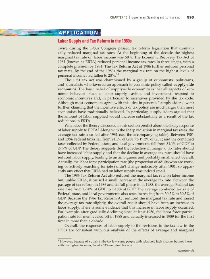
Labor Supply and Tax reform in the 1980sTwice during the 1980s Congress passed tax reform legislation that dramati-cally reduced marginal tax rates. At the beginning of the decade the highest marginal tax rate on labor income was 50%. The Economic Recovery Tax Act of 1981 (known as ERTA) reduced personal income tax rates in three stages, with a complete phase-in by 1984. The Tax Reform Act of 1986 further reduced personal tax rates. By the end of the 1980s the marginal tax rate on the highest levels of personal income had fallen to 28%.10
The 1981 tax act was championed by a group of economists, politicians, and journalists who favored an approach to economic policy called supply-side economics. The basic belief of supply-side economics is that all aspects of eco-nomic behavior—such as labor supply, saving, and investment—respond to economic incentives and, in particular, to incentives provided by the tax code. Although most economists agree with this idea in general, “supply-siders” went further, claiming that the incentive effects of tax policy are much larger than most economists have traditionally believed. In particular, supply-siders argued that the amount of labor supplied would increase substantially as a result of the tax reductions in ERTA.
What does the theory discussed in this section predict about the likely response of labor supply to ERTA? Along with the sharp reduction in marginal tax rates, the average tax rate also fell after 1981 (see the accompanying table). Between 1981 and 1984 Federal taxes fell from 21.1% of GDP to 19.2% of GDP, and the combined taxes collected by Federal, state, and local governments fell from 31.1% of GDP to 29.7% of GDP. The theory suggests that the reduction in marginal tax rates should have increased labor supply and that the decline in average tax rates should have reduced labor supply, leading to an ambiguous and probably small effect overall. Actually, the labor force participation rate (the proportion of adults who are work-ing or actively searching for jobs) didn’t change noticeably after 1981, so appar-ently any effect that ERTA had on labor supply was indeed small.
The 1986 Tax Reform Act also reduced the marginal tax rate on labor income but, unlike ERTA, it caused a small increase in the average tax rate. Between the passage of tax reform in 1986 and its full phase-in in 1988, the average Federal tax rate rose from 19.4% of GDP to 19.8% of GDP. The average combined tax rate of Federal, state, and local governments also rose, increasing from 30.2% to 30.5% of GDP. Because the 1986 Tax Reform Act reduced the marginal tax rate and raised the average tax rate slightly, the overall result should have been an increase in labor supply. There is some evidence that this increase in labor supply occurred. For example, after gradually declining since at least 1950, the labor force partici-pation rate for men leveled off in 1988 and actually increased in 1989 for the first time in more than a decade.
Overall, the responses of labor supply to the revisions to the tax law in the 1980s are consistent with our analysis of the effects of average and marginal
10However, because of a quirk in the tax law, some people with relatively high income, but not those with the highest incomes, faced a 33% marginal tax rate.
(continued)
594 parT 4 | Macroeconomic Policy: Its Environment and Institutions
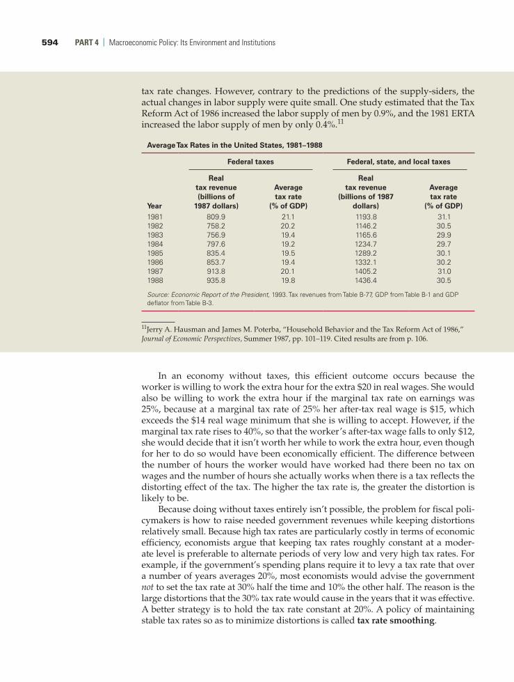
tax rate changes. However, contrary to the predictions of the supply-siders, the actual changes in labor supply were quite small. One study estimated that the Tax Reform Act of 1986 increased the labor supply of men by 0.9%, and the 1981 ERTA increased the labor supply of men by only 0.4%.11
Average Tax Rates in the United States, 1981–1988
Federal taxes Federal, state, and local taxes
Year
Real tax revenue (billions of
1987 dollars)
Average tax rate
(% of GDP)
Real tax revenue
(billions of 1987 dollars)
Average tax rate
(% of GDP)1981 809.9 21.1 1193.8 31.11982 758.2 20.2 1146.2 30.51983 756.9 19.4 1165.6 29.91984 797.6 19.2 1234.7 29.71985 835.4 19.5 1289.2 30.11986 853.7 19.4 1332.1 30.21987 913.8 20.1 1405.2 31.01988 935.8 19.8 1436.4 30.5
Source: Economic Report of the President, 1993. Tax revenues from Table B-77, GDP from Table B-1 and GDP deflator from Table B-3.
In an economy without taxes, this efficient outcome occurs because the worker is willing to work the extra hour for the extra $20 in real wages. She would also be willing to work the extra hour if the marginal tax rate on earnings was 25%, because at a marginal tax rate of 25% her after-tax real wage is $15, which exceeds the $14 real wage minimum that she is willing to accept. However, if the marginal tax rate rises to 40%, so that the worker’s after-tax wage falls to only $12, she would decide that it isn’t worth her while to work the extra hour, even though for her to do so would have been economically efficient. The difference between the number of hours the worker would have worked had there been no tax on wages and the number of hours she actually works when there is a tax reflects the distorting effect of the tax. The higher the tax rate is, the greater the distortion is likely to be.
Because doing without taxes entirely isn’t possible, the problem for fiscal poli-cymakers is how to raise needed government revenues while keeping distortions relatively small. Because high tax rates are particularly costly in terms of economic efficiency, economists argue that keeping tax rates roughly constant at a moder-ate level is preferable to alternate periods of very low and very high tax rates. For example, if the government’s spending plans require it to levy a tax rate that over a number of years averages 20%, most economists would advise the government not to set the tax rate at 30% half the time and 10% the other half. The reason is the large distortions that the 30% tax rate would cause in the years that it was effective. A better strategy is to hold the tax rate constant at 20%. A policy of maintaining stable tax rates so as to minimize distortions is called tax rate smoothing.
11Jerry A. Hausman and James M. Poterba, “Household Behavior and the Tax Reform Act of 1986,” Journal of Economic Perspectives, Summer 1987, pp. 101–119. Cited results are from p. 106.

ChapTer 15 | Government Spending and Its Financing 595
Has the Federal government had a policy of tax rate smoothing? Statistical studies typically have found that Federal tax rates are affected by political and other factors and hence aren’t as smooth as is necessary to minimize distortions.12 Nevertheless, the idea of tax smoothing is still useful. For example, what explains the U.S. government’s huge deficit during World War II (Fig. 15.4)? The alterna-tive to deficit financing of the war would have been a large wartime increase in tax rates, coupled with a drop in tax rates when the war was over. But high tax rates during the war would have distorted the economy when productive ef-ficiency was especially important. By financing the war through borrowing, the government effectively spread the needed tax increase over a long period of time (as the debt was repaid) rather than raising current taxes by a large amount. This action is consistent with the idea of tax smoothing.
12David Bizer and Steven Durlauf, “Testing the Positive Theory of Government Finance,” Journal of Monetary Economics, August 1990, pp. 123–141.
The single number in the Federal government’s budget that is the focus of most public attention is the size of the budget deficit or surplus. During the 1980s and early 1990s, large deficits led to vigorous public debate about the potential impact of big deficits on the economy, and this debate was reignited following the recent financial crisis, as the budget deficit averaged almost 9% of GDP from 2009 to 2011. In the rest of this chapter we discuss the government budget deficit, the gov-ernment debt, and their effects on the economy.
The Growth of the Government DebtThere is an important distinction between the government budget deficit and the government debt (also called the national debt). The government budget deficit (a flow variable) is the difference between expenditures and tax revenues in any fiscal year. The government debt (a stock variable) is the total value of govern-ment bonds outstanding at any particular time. Because the excess of government expenditures over revenues equals the amount of new borrowing that the govern-ment must do—that is, the amount of new government debt that it must issue—any year’s deficit (measured in dollar, or nominal, terms) equals the change in the debt in that year. We can express the relationship between government debt and the budget deficit by
∆B = nominal government budget deficit, (15.3)
where ∆B is the change in the nominal value of government bonds outstanding.In a period of persistently large budget deficits, such as that experienced by
the United States in the 1980s and early and mid-1990s, and again after 2002, the nominal value of the government’s debt will grow quickly. For example, between 1980 and 2011, Federal government debt held by the public grew by over four-teen times in nominal terms, from $712 billion in 1980 to $10,128 billion in 2011.13 Taking inflation into account, the real value of government debt outstanding in-creased nearly six-fold during this period.
15.3 Government Deficits and DebtDiscuss the economic effects of government deficits and debt.
13Economic Report of the President, Table B-78, www.whitehouse.gov/administration/eop/cea/economic-report-of-the-President.
596 parT 4 | Macroeconomic Policy: Its Environment and Institutions
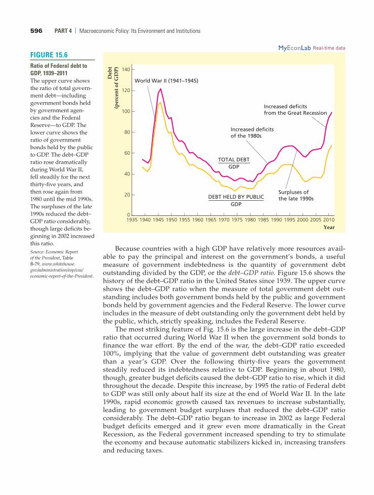
Because countries with a high GDP have relatively more resources avail-able to pay the principal and interest on the government’s bonds, a useful measure of government indebtedness is the quantity of government debt outstanding divided by the GDP, or the debt–GDP ratio. Figure 15.6 shows the history of the debt–GDP ratio in the United States since 1939. The upper curve shows the debt–GDP ratio when the measure of total government debt out-standing includes both government bonds held by the public and government bonds held by government agencies and the Federal Reserve. The lower curve includes in the measure of debt outstanding only the government debt held by the public, which, strictly speaking, includes the Federal Reserve.
The most striking feature of Fig. 15.6 is the large increase in the debt–GDP ratio that occurred during World War II when the government sold bonds to finance the war effort. By the end of the war, the debt–GDP ratio exceeded 100%, implying that the value of government debt outstanding was greater than a year’s GDP. Over the following thirty-five years the government steadily reduced its indebtedness relative to GDP. Beginning in about 1980, though, greater budget deficits caused the debt–GDP ratio to rise, which it did throughout the decade. Despite this increase, by 1995 the ratio of Federal debt to GDP was still only about half its size at the end of World War II. In the late 1990s, rapid economic growth caused tax revenues to increase substantially, leading to government budget surpluses that reduced the debt–GDP ratio considerably. The debt–GDP ratio began to increase in 2002 as large Federal budget deficits emerged and it grew even more dramatically in the Great Recession, as the Federal government increased spending to try to stimulate the economy and because automatic stabilizers kicked in, increasing transfers and reducing taxes.
FiGure 15.6ratio of Federal debt to GDp, 1939–2011The upper curve shows the ratio of total govern-ment debt—including government bonds held by government agen-cies and the Federal Reserve—to GDP. The lower curve shows the ratio of government bonds held by the public to GDP. The debt–GDP ratio rose dramatically during World War II, fell steadily for the next thirty-five years, and then rose again from 1980 until the mid 1990s. The surpluses of the late 1990s reduced the debt– GDP ratio considerably, though large deficits be-ginning in 2002 increased this ratio.Source: Economic Report of the President, Table B-79, www.whitehouse.gov/administration/eop/cea/economic-report-of-the-President.
0
20
40
60
80
100
120
140
1935 1940 1945 1950 1955 1960 1965 1970 1975 1980 1985 1990 1995 2000 2005 2010
Deb
t(p
erce
nt o
f G
DP
)
Year
TOTAL DEBTGDP
DEBT HELD BY PUBLICGDP
World War II (1941–1945)
Increased deficitsof the 1980s
Surpluses ofthe late 1990s
Increased deficitsfrom the Great Recession
MyEconLab Real-time data
ChapTer 15 | Government Spending and Its Financing 597
We can describe changes in the debt–GDP ratio over time by the following formula (derived in Appendix 15.A at the end of the chapter):
change indebt@GDP ratio
=deficit
nominal GDP- a total debt
nominal GDP*
growth rate ofnominal GDP
b (15.4)
Equation (15.4) emphasizes two factors that cause the debt–GDP ratio to rise quickly:
■■ a high deficit relative to GDP and■■ a slow rate of GDP growth.
Equation (15.4) helps account for the pattern of the debt–GDP ratio shown in Fig. 15.6. The sharp increase during World War II was the result of large deficits. In contrast, for the three and a half decades after World War II, the Federal gov-ernment’s deficit was small and GDP growth was rapid, so the debt–GDP ratio declined. The debt–GDP ratio increased during the 1980s and early 1990s because the Federal deficit was high. Large surpluses helped reduce the debt–GDP ratio in the late 1990s, but large deficits beginning in 2002 and increasing during the Great Recession have reversed the decline in the debt–GDP ratio. One factor affecting the debt–GDP ratio is the Social Security system, discussed in the Application “Social Security: How Can It Be Fixed?”
A P P l I C AT I o n
Social Security: how Can it Be Fixed?The Social Security system was created in 1937, during the administration of President Franklin D. Roosevelt, to provide income to retired workers. Since then, the program has been expanded to include payments to survivors of deceased workers (in 1939) and to people unable to work because of a disability (in 1954).14 Recently, Social Security has been the focus of much attention because projections suggest that, unless the program is reformed, it will be unable to pay promised benefits to future retirees.
Social Security today is largely a pay-as-you-go system, which means that most of the payroll taxes that workers and their employers pay in go directly to retirees and other beneficiaries. The portion of payroll tax revenue not used to fund the benefits of current beneficiaries is spent by the Federal government on other programs. To keep track of its obligations to the Social Security system, the government credits the system account, known as the Social Security trust fund, with special govern-ment bonds (IOUs) equal to the amount of payroll taxes spent on other programs. In the future, when Social Security payroll taxes are no longer sufficient to fund contemporaneous Social Security benefits, much of the difference will be made up by redeeming bonds from the trust fund. In practice, the government will be able to pay off these bonds only by raising taxes or cutting spending on other programs.
As long as the number of workers paying into Social Security greatly exceeded the number of retirees and other beneficiaries, the system could finance 14For more details, see Thomas A. Garrett and Russell M. Rhine, “Social Security versus Private Retirement Accounts: An Analysis,” pt. 1, Federal Reserve Bank of St. Louis, Review, March/April 2005, pp. 103–121.
(continued)

598 parT 4 | Macroeconomic Policy: Its Environment and Institutions
itself on a pay-as-you-go basis, with any excess Social Security tax revenue added to the Social Security trust fund. However, the ratio of workers to retirees is ex-pected to decrease significantly in the coming decades, reflecting the impending retirement of the baby boomers (the large cohort of people born in the years im-mediately after World War II), declining U.S. birth rates, and longer life expectan-cies (which mean that people spend many more years in retirement than they used to). Figure 15.7 shows that since 2010 the Social Security system has taken in less in tax revenue than it spent. Without a major change in the system, payouts from the system will continue to exceed the revenue into the system for the fore-seeable future. The projections show that payouts as a percent of GDP begin to rise sharply in 2019 and continue to rise over the subsequent 15 years, as the baby boomers retire and collect benefits. For a while, the Social Security system can use its interest earnings and redeem bonds in the Social Security trust fund to be able to pay benefits that exceed tax revenue each year. But if the system is not modi-fied, the trustees estimate that the trust fund will be exhausted in 2033 and the system will no longer be able to pay currently promised benefits.
Fixing the Social Security SystemSeveral proposals to fix the Social Security system have been suggested. The pro-posals include increasing tax revenue coming into the system, earning a higher rate of return on the Social Security trust fund, and reducing benefit payments made by Social Security. Tax revenue could be increased by raising Social Security payroll taxes or by subjecting more income to the tax, but both would distort workers’ labor supply decisions. The rate of return on the Social Security trust FiGure 15.7
Social Security payout and tax revenue as a percent of GDp, 1990–2090The figure shows annual values for the cost of providing benefits and the tax revenue collected by the Social Security system each year from 1990 to 2011 and the projected payout and tax revenue from 2012 to 2090. Benefits payments will soon begin to rise sharply compared with tax revenue, a develop-ment that will create fi-nancial problems for the system.Source: The 2012 Annual Report of the Board of Trustees of the Federal Old-Age and Survivors Insurance and Federal Disability Insurance Trust Funds, available at www.socialsecurity.gov/OACT/TR/2012/LD_figIID4.html.
0
1
2
3
4
5
6
7
1990 2000 2010 2020 2030 2040 2050 2060 2070 2080 2090
Per
cen
t of
GD
P
Year
TAX REVENUE
PAYOUT
ACTUAL PROJECTED
ChapTer 15 | Government Spending and Its Financing 599
The Burden of the Government Debt on Future GenerationsPeople often express concern that the trillions of dollars of Federal government debt will impose a crushing financial burden on their children and grandchildren, who will someday be taxed to pay off these debts. In this view, high rates of gov-ernment borrowing amount to “robbing the future” to pay for government spend-ing that is too high or taxes that are too low in the present.
Until recently, it was reasonable to argue that most U.S. government bonds are owned by U.S. citizens. Therefore, although our descendants someday may face heavy taxes to pay the interest and principal of the government debt, these future taxpayers also will inherit outstanding government bonds and thus will be the recipients of most of those interest and principal payments. In that case, one could argue that to a substantial degree, we owe the government debt to our-selves, so the debt isn’t a burden in the same sense that it would be if it were owed entirely to outsiders. However, over the past 20 years, investors, institutions, and governments in other countries—most notably, China—have bought large amounts of U.S. government debt. Since 2005, foreigners have owned more than half of all publicly owned U.S. government debt. So, the argument that the debt is not a burden because we owe it to ourselves is no longer valid.
Although the popular view of the burden of the government debt is faulty, economists have pointed out several ways in which the government debt can become a burden on future generations. First, if tax rates have to be raised
fund could be increased by allowing the government to invest the trust fund in the stock market, but this would clearly increase the risk to the trust fund’s return, and could lead to government interference in the stock market. Benefit payments could be reduced by raising the age at which benefits could be collected (to match the increase in life expectancy), or by changing the formula relating benefits to the average increase in wages and prices.
Another controversial proposal would allow people (on a voluntary basis) to invest some portion of their Social Security taxes in individual accounts that could include well-diversified mutual funds that hold stocks. Such individual accounts would allow workers some control over their retirement funds and how they are invested.
An objection to individual accounts arises from the fact that, under a pay-as-you-go system, Social Security payroll taxes are used to fund benefits to current retirees. Thus if payroll taxes are directed toward individual accounts, the govern-ment will not receive sufficient revenue to pay current benefits and would have to increase tax rates or borrow the difference, increasing the amount of govern-ment debt that is issued. So individual accounts could be a useful component of a comprehensive overhaul of the Social Security system, but by themselves they are unlikely to eradicate the projected shortfall facing the current system.
Do we really need to worry about Social Security now? Or can we just wait until 2033 and see if the Social Security system runs out of funds? Most experts seem to think that the demographic trends are very clear and that the system is in trouble. If, indeed, the Social Security system needs to be fixed, then the longer we wait to reform it, the more drastic will be the changes that are ultimately required to restore solvency to the system.
600 parT 4 | Macroeconomic Policy: Its Environment and Institutions
substantially in the future to pay off the debt, the resulting distortions could cause the economy to function less efficiently and impose costs on future generations.
Second, most people hold small amounts of government bonds or no govern-ment bonds at all (except perhaps indirectly, as through pension funds). In the future, people who hold few or no bonds may have to pay more in taxes to pay off the government debt than they receive in interest and principal payments; people holding large quantities of bonds may receive more in interest and principal than they pay in increased taxes. Bondholders are richer on average than nonbond-holders, so the need to service the government debt might lead to a transfer of resources from the relatively poor to the relatively rich. However, this transfer could be offset by other tax and transfer policies—for example, by raising taxes on high-income people.
The third argument is probably the most significant: Many economists claim that government deficits reduce national saving; that is, when the government runs a deficit, the economy accumulates less domestic capital and fewer foreign assets than it would have if the deficit had been lower. If this argument is correct, deficits will lower the standard of living for our children and grandchildren, both because they will inherit a smaller capital stock and because they will have to pay more interest to (or receive less interest from) foreigners than they otherwise would have. This reduction in the future standard of living would constitute a true burden of the government debt.
Crucial to this argument, however, is the idea that government budget defi-cits reduce national saving. As we have mentioned at several points in this book (notably in Chapter 4), the question of whether budget deficits affect national saving is highly controversial. We devote most of the rest of this section to further discussion of this issue.
Budget Deficits and National Saving: ricardian equivalence revisitedUnder what circumstances will an increased government budget deficit cause national saving to fall? Virtually all economists agree that an increase in the deficit caused by a rise in government purchases—say, to fight a war—reduces national saving and imposes a real burden on the economy. However, whether a deficit caused by a cut in current taxes or an increase in current transfers reduces na-tional saving is much less clear. Recall that advocates of Ricardian equivalence ar-gue that tax cuts or increases in transfers will not affect national saving, whereas its opponents disagree.
ricardian equivalence: an example. To illustrate Ricardian equivalence let’s suppose that, holding its current and planned future purchases constant, the gov-ernment cuts this year’s taxes by $100 per person. (Assuming that the tax cut is a lump sum allows us to ignore incentive effects.) What impact will this reduction in taxes have on national saving? In answering this question, we first recall the definition of national saving (Eq. 2.8):
S = Y - C - G. (15.5)
Equation (15.5) states that national saving, S, equals output, Y, less consumption, C, and government purchases, G.15 If we assume that government purchases, G,
15We assume that net factor payments from abroad, NFP, are zero.

ChapTer 15 | Government Spending and Its Financing 601
are constant and that output, Y, is fixed at its full-employment level, we know from Eq. (15.5) that the tax cut will reduce national saving, S, only if it causes consumption, C, to rise. Advocates of Ricardian equivalence assert that, if current and planned future government purchases are unchanged, a tax cut will not affect consumption and thus won’t affect national saving.
Why wouldn’t a tax cut that raises after-tax incomes cause people to consume more? The answer is that—if current and planned future government purchases don’t change—a tax cut today must be accompanied by an offsetting increase in expected future taxes. To see why, note that if current taxes are reduced by $100 per person without any change in government purchases, the government must borrow an additional $100 per person by selling bonds. Suppose that the bonds are one-year bonds that pay a real interest rate, r. In the following year, when the gov-ernment repays the principal ($100 per person) and interest ($100 * r per person) on the bonds, it will have to collect an additional +100(1 + r) per person in taxes. Thus, when the public learns of the current tax cut of $100 per person, they should also expect their taxes to increase by +100(1 + r) per person next year.16
Because the current tax cut is balanced by an increase in expected future taxes, it doesn’t make taxpayers any better off in the long run despite raising their current after-tax incomes. Indeed, after the tax cut, taxpayers’ abilities to consume today and in the future are the same as they were originally. That is, if no one consumes more in response to the tax cut—so that each person saves the entire $100 increase in after-tax income—in the following year the $100 per person of additional sav-ing will grow to +100(1 + r) per person. This additional +100(1 + r) per person is precisely the amount needed to pay the extra taxes that will be levied in the future, leaving people able to consume as much in the future as they had origi-nally planned. Because people aren’t made better off by the tax cut (which must be coupled with a future tax increase), they have no reason to consume more today. Thus national saving should be unaffected by the tax cut, as supporters of Ricardian equivalence claim.
ricardian equivalence across Generations. The argument for Ricardian equivalence rests on the assumption that current government borrowing will be repaid within the lifetimes of people who are alive today. In other words, any tax cuts received today are offset by the higher taxes that people must pay later. But what if some of the debt the government is accumulating will be repaid not by the people who receive the tax cut but by their children or grandchildren? In that case, wouldn’t people react to a tax cut by consuming more?
Harvard economist Robert Barro17 has shown that, in theory, Ricardian equivalence may still apply even if the current generation receives the tax cut and future generations bear the burden of repaying the government’s debt. To state Barro’s argument in its simplest form, let’s imagine an economy in which every generation has the same number of people and suppose that the current genera-tion receives a tax cut of $100 per person. With government purchases held con-stant, this tax cut increases the government’s borrowing and outstanding debt by
16The government might put the tax increase off for two, three, or more years. Nevertheless, the gen-eral conclusion that the current tax cut must be offset by future tax increases would be unchanged.17“Are Government Bonds Net Wealth?” Journal of Political Economy, November/December 1974, pp. 1095–1117.

602 parT 4 | Macroeconomic Policy: Its Environment and Institutions
$100 per person. However, people currently alive are not taxed to repay this debt; instead, this obligation is deferred until the next generation. To repay the govern-ment’s increased debt, the next generation’s taxes (in real terms) will be raised by +100(1 + r) per person, where 1 + r is the real value of a dollar borrowed today at the time the debt is repaid.18
Seemingly, the current generation of people, who receive the tax cut, should increase their consumption because the reduction in their taxes isn’t expected to be balanced by an increase in taxes during their lifetimes. However, Barro argued that people in the current generation shouldn’t increase their consumption in response to a tax cut if they care about the well-being of the next generation. Of course, people do care about the well-being of their children, as is reflected in part in the economic resources devoted to children, including funds spent on chil-dren’s health and education, gifts, and inheritances.
How does the concern of this generation for the next affect the response of people to a tax cut? A member of the current generation who receives a tax cut—call him Joe—might be inclined to increase his own consumption, all else being equal. But, Barro argues, Joe should realize that, for each dollar of tax cut he receives today, his son Joe Junior will have to pay 1 + r dollars of extra taxes in the future. Can Joe do anything on his own to help out Joe Junior? The answer is yes. Suppose that, instead of consuming his $100 tax cut, Joe saves the $100 and uses the extra savings to increase Joe Junior’s inheritance. By the time the next generation is required to pay the government debt, Joe Junior’s ex-tra inheritance plus accumulated interest will be +100(1 + r), or just enough to cover the increase in Joe Junior’s taxes. Thus, by saving his tax cut and adding these savings to his planned bequest, Joe can keep both his own consumption and Joe Junior’s consumption the same as they would have been if the tax cut had never occurred.
Furthermore, Barro points out, Joe should save all his tax cut for Joe Junior’s benefit. Why? If Joe consumes even part of his tax cut, he won’t leave enough extra inheritance to allow Joe Junior to pay the expected increase in his taxes, and so Joe Junior will have to consume less than he could have if there had been no tax cut for Joe. But if Joe wanted to increase his own consumption at Joe Junior’s expense, he could have done so without changes in the tax laws—for example, by contribut-ing less to Joe Junior’s college tuition payments or by planning to leave a smaller inheritance. That Joe didn’t take these actions shows that he was satisfied with the division of consumption between himself and Joe Junior that he had planned before the tax cut was enacted; there is no reason that the tax cut should cause this original consumption plan to change. Therefore if Joe and other members of the current generation don’t consume more in response to a tax cut, Ricardian equiva-lence should hold even when debt repayment is deferred to the next generation.
This analysis can be extended to allow for multiple generations and in other ways. These extensions don’t change the main point, which is that, if taxpayers understand that they are ultimately responsible for the government’s debt, they shouldn’t change their consumption in response to changes in taxes or transfers that are unaccompanied by changes in planned government purchases. As a re-sult, deficits created by tax cuts shouldn’t reduce national saving and therefore shouldn’t burden future generations.
18For example, if the debt is to be repaid in thirty years and r is the one-year real interest rate, then 1 + r = (1 + r)30.

ChapTer 15 | Government Spending and Its Financing 603
Departures from ricardian equivalenceThe arguments for Ricardian equivalence are logically sound, and this idea has greatly influenced economists’ thinking about deficits. Although forty years ago most economists would have taken for granted that a tax cut would sub-stantially increase consumption, today there is much less agreement about this claim. Although Ricardian equivalence seemed to fail spectacularly in the 1980s in the United States—when high government budget deficits were accompanied by extremely low rates of national saving—data covering longer periods of time suggest little relationship between budget deficits and national saving rates in the United States. In some other countries, such as Canada and Israel, Ricardian equivalence seems to have worked quite well at times.19
Our judgment is that tax cuts that lead to increased government borrowing probably affect consumption and national saving, although the effect may be small. We base this conclusion both on the experience of the United States dur-ing the 1980s and on the fact that there are some theoretical reasons to expect Ricardian equivalence not to hold exactly. The main arguments against Ricardian equivalence are the possible existence of borrowing constraints, consumers’ short-sightedness, the failure of some people to leave bequests, and the non-lump-sum nature of most tax changes.
1. Borrowing constraints. Many people would be willing to consume more if they could find lenders who would extend them credit. However, consumers often face limits, known as borrowing constraints, on the amounts that they can bor-row. A person who wants to consume more, but who is unable to borrow to do so, will be eager to take advantage of a tax cut to increase consumption. Thus the existence of borrowing constraints may cause Ricardian equivalence to fail.
2. Shortsightedness. In the view of some economists, many people are short-sighted and don’t understand that as taxpayers they are ultimately respon-sible for the government’s debt. For example, some people may determine their consumption by simple “rules of thumb,” such as the rule that a family should spend fixed percentages of its current after-tax income on food, cloth-ing, housing, and so on, without regard for how its income is likely to change in the future. If people are shortsighted, they may respond to a tax cut by con-suming more, contrary to the prediction of Ricardian equivalence. However, Ricardians could reply that ultrasophisticated analyses of fiscal policy by consumers aren’t necessary for Ricardian equivalence to be approximately correct. For example, if people know generally that big government deficits mean future problems for the economy (without knowing exactly why), they may be reluctant to spend from a tax cut that causes the deficit to balloon, consistent with the Ricardian prediction.
3. Failure to leave bequests. If people don’t leave bequests, perhaps because they don’t care or think about the long-run economic welfare of their children, they will increase their consumption if their taxes are cut, and Ricardian
19For surveys of the evidence by a supporter and an opponent of Ricardian equivalence, respectively, see Robert Barro, “The Ricardian Approach to Budget Deficits,” Journal of Economic Perspectives, Spring 1989, pp. 37–54; and B. Douglas Bernheim, “Ricardian Equivalence: An Evaluation of Theory and Evidence,” in Stanley Fischer, ed., NBER Macroeconomics Annual, Cambridge, Mass.: M.I.T. Press, 1987.

604 parT 4 | Macroeconomic Policy: Its Environment and Institutions
equivalence won’t hold. Some people may not leave bequests because they expect their children to be richer than they are and thus not need any bequest. If people continue to hold this belief after they receive a tax cut, they will in-crease their consumption and again Ricardian equivalence will fail.
4. Non-lump-sum taxes. In theory, Ricardian equivalence holds only for lump-sum tax changes, with each person’s change in taxes being a fixed amount that doesn’t depend on the person’s economic decisions, such as how much to work or save. As discussed in Section 15.2, when taxes are not lump-sum, the level and timing of taxes will affect incentives and thus economic behavior. Thus non-lump-sum tax cuts will have real effects on the economy, in contrast to the simple Ricardian view.
We emphasize, though, that with non-lump-sum taxes, the incentive effects of a tax cut on consumption and saving behavior will depend heavily on the tax structure and on which taxes are cut. For example, a temporary cut in sales taxes would likely stimulate consumption, but a reduction in the tax rate on interest earned on savings accounts might increase saving. Thus we cannot always conclude that, just because taxes aren’t lump-sum, a tax cut will increase consumption. That conclusion has to rest primarily on the other three arguments against Ricardian equivalence that we presented.
I n T o U C h w I T h D A T A A n D R e S e A R C h
Measuring the impact of Government purchases on the economyIn February 2009, the U.S. government enacted The American Recovery and Reinvestment Act of 2009 with the aim of lifting the economy out of the recession that began in December 2007. This bill, which is often called a stimulus package, was projected to increase the Federal government’s deficit by nearly $800 billion over the following decade, by reducing taxes by about $300 billion and increas-ing government expenditures by about $500 billion. At the time, classical and Keynesian economists engaged in a vigorous debate about the impact of the stimulus package on the economy by looking at past historical episodes and using a variety of empirical methods.
In the IS–LM model, a temporary increase in government purchases shifts the IS curve up and to the right (as discussed on pp. 322–323), which causes the IS–LM intersection to move upward and rightward also. In the Keynesian version of the model, prices remain fixed in the short run and the upward and rightward shift of the IS–LM intersection indicates output increases in the short run. In the classical version of the model, however, prices adjust quickly, thereby shifting the LM curve up and to the left, which tends to offset the rightward shift of the IS curve. However, there is an alternative channel by which a temporary increase in government purchases will increase output in the classical model. Recall that in the classical model, as discussed in Chapter 10, pp. 378–382, an increase in government purchases is equivalent to a decrease in people’s wealth, as current or future taxes must increase to pay for the additional government spending. The wealth effect causes people to increase their labor supply, increasing output. Thus, in both Keynesian and classical models, temporary increases in government purchases lead to higher output, though the mechanisms differ in the two models.

ChapTer 15 | Government Spending and Its Financing 605
It is not an easy matter to calculate the size of the multiplier associated with particular changes in government purchases—even after the fact—because so many other shocks may hit the economy and affect output. Economist Valerie Ramey of the University of California at San Diego evaluated research on the size of the government spending multiplier performed over the past 40 years.20 You may recall from Chapter 11, pp. 426–427, that the multiplier is the short-run change in output that arises from a one unit change in government purchases. The general finding of the research that Ramey reviewed is that for a deficit-financed temporary increase in government purchases, which describes part of the 2009 stimulus package, the government spending multiplier is likely to be between 0.8 and 1.5. So, a temporary increase in government purchases of $100 billion would increase GDP by between $80 billion and $150 billion.
Ramey’s evidence was based on a large number of studies of the government spending multiplier in many different situations. But you might think that the multiplier is higher when the economy is in a recession, when there are many unemployed resources, than when it is in an expansion. In a recent study, Alan J. Auerbach and Yuriy Gorodnichenko, both of the University of California at Berkeley, examined the government spending multiplier using a model that al-lows for the economy to be in one of two regimes: expansion or recession.21 They find that the multiplier is only about 0 to 0.5 in economic expansions but much higher, 1 to 1.5, in recessions.
The impact of government spending on the economy may also be affected by the response of monetary policy. Research by Gauti Eggertsson of the Federal Reserve Bank of New York finds that the government spending multiplier may be substantially higher if monetary policy is constrained by being at the zero lower bound (see Chapter 14, pp. 561–564, for a discussion), as it has been in recent years in the United States.22
So, the empirical evidence indicates that temporary increases in government purchases can increase output with a multiplier between 0.8 and 1.5. The multi-plier is higher if the economy is in a recession rather than in an expansion, and higher still if monetary policy is constrained by being at the zero lower bound.
20“Can Government Purchases Stimulate the Economy?” Journal of Economic Literature (September 2011), pp. 673–685.21“Measuring the Output Responses to Fiscal Policy,” American Economic Journal: Economic Policy (March 2012), pp. 1–27.22“What Fiscal Policy Is Effective at Zero Interest Rates?” NBER Macroeconomics Annual 2010, Daron Acemoglu and Michael Woodford, editors (Chicago: University of Chicago Press, 2011), pp. 59–112.
In this final section of the chapter we discuss one more concern that has been expressed about government budget deficits: that deficits are inflationary. We show that the principal link between deficits and inflation is that in some circum-stances deficits lead to higher rates of growth in the money supply and that high rates of money growth in turn cause inflation.
15.4 Deficits and inflationExplain the link between deficits and inflation.

606 parT 4 | Macroeconomic Policy: Its Environment and Institutions
The Deficit and the Money SupplyInflation—a rising price level—results when aggregate demand increases more quickly than does aggregate supply. In terms of the AD–AS framework, suppose that the long-run aggregate supply curve (which reflects the productive capacity of the economy) is fixed. Then for the price level to rise, the aggregate demand curve must rise over time.
Both the classical and Keynesian models of the economy imply that deficits can cause aggregate demand to rise more quickly than aggregate supply, lead-ing to an increase in the price level. In both models a deficit owing to increased government purchases reduces desired national saving, shifting the IS curve up and to the right and causing aggregate demand to rise. This increase in aggregate demand causes the price level to rise.23 If we assume (as Keynesians usually do) that Ricardian equivalence doesn’t hold, a budget deficit resulting from a cut in taxes or an increase in transfers also reduces desired national saving, increases aggregate demand, and raises the price level. Thus deficits resulting from expan-sionary fiscal policies (increased spending or reduced taxes) will be associated with inflation.
However, an increase in government purchases or a cut in taxes causes only a one-time increase in aggregate demand. Therefore, although we expect expansionary fiscal policies to lead to a one-time increase in the price level (that is, a temporary burst in inflation), we don’t expect an increase in government purchases or a cut in taxes to cause a sustained increase in inflation. In general, the only factor that can sustain an increase in aggregate demand, leading to con-tinuing inflation, is sustained growth in the money supply. Indeed, high rates of inflation are almost invariably linked to high rates of national money growth (recall the Application “Money Growth and Inflation in European Countries in Transition,” pp. 269–270). The key question therefore is: Can government budget deficits lead to ongoing increases in the money supply?
The answer is “yes.” The link is the printing of money to finance government spending when the government cannot (or does not want to) finance all of its spending by taxes or borrowing from the public. In the extreme case, imagine a government that wants to spend $10 billion (say, on submarines) but has no abil-ity to tax or borrow from the public. One option is for this government to print $10 billion worth of currency and use this currency to pay for the submarines. The revenue that a government raises by printing money is called seignorage. Any government with the authority to issue money can use seignorage; governments that do not have the authority to issue money, such as state governments in the United States, can’t use seignorage.
Actually, governments that want to finance their deficits through seignorage don’t simply print new currency but use an indirect procedure. First, the Treasury authorizes government borrowing equal to the amount of the budget deficit ($10 billion in our example), and a corresponding quantity of new government bonds is printed and sold. Thus the deficit still equals the change in the outstand-ing government debt (Eq. 15.3). However, the new government bonds aren’t sold to the public. Instead, the Treasury asks (or requires) the central bank to purchase the $10 billion in new bonds. The central bank pays for its purchases of new
23The classical analysis predicts that an increase in government purchases will cause aggregate sup-ply to rise as well, but we have assumed that the supply effect is smaller than the demand effect.
ChapTer 15 | Government Spending and Its Financing 607
bonds by printing $10 billion in new currency,24 which it gives to the Treasury in exchange for the bonds. This newly issued currency enters general circulation when the government spends it on its various outlays (the submarines). Note that the purchase of bonds by the central bank increases the monetary base by the amount of the purchase (see Chapter 14), as when the central bank purchases government bonds on the open market.
The precise relationship between the size of the deficit and the increase in the monetary base is
deficit = ∆B = ∆Bp + ∆Bcb = ∆Bp + ∆BASE. (15.6)
Equation (15.6) states that the (nominal) government budget deficit equals the total increase in (nominal) government debt outstanding, ∆B, which can be broken into additional government debt held by the public, ∆Bp, and by the cen-tral bank, ∆Bcb. The increase in government debt held by the central bank in turn equals the increase in the monetary base, ∆BASE. The increase in the monetary base equals the amount of seignorage collected by the government.
The final link between the budget deficit and the money supply has to do with the relationship between the money supply and the monetary base. To make the link as simple as possible, we consider an all-currency economy. Specifically, in an all-currency economy there are no banks, and all money is held in the form of currency. In an all-currency economy, the money supply equals the amount of currency outstanding (because there are no deposits) and the monetary base equals the amount of currency outstanding (because there are no bank reserves), so the money supply and the monetary base are equal. Therefore, in an all-cur-rency economy, Eq. (15.6) implies that
deficit = ∆B = ∆Bp + ∆Bcb = ∆Bp + ∆M, (15.7)
where ∆BASE = ∆M.Why would governments use seignorage to finance their deficits, knowing that
continued money creation ultimately leads to inflation? Under normal conditions developed countries rarely use seignorage. For example, in recent years (preceding the financial crisis of 2008) the monetary base in the United States increased on average by about $40 billion per year, which equals about 2% of Federal govern-ment receipts. Heavy reliance on seignorage usually occurs in war-torn or develop-ing countries, in which military or social conditions dictate levels of government spending well above what the country can raise in taxes or borrow from the public.
real Seignorage Collection and inflationThe amount of real revenue that the government collects from seignorage is closely related to the inflation rate. To examine this link let’s consider an all-currency economy in which real output and the real interest rate are fixed and the rates of money growth and inflation are constant. In such an economy the real quantity of money demanded is constant25 and hence, in equilibrium, the real
24The new money created by the central bank could also be in the form of deposits at the central bank; the ultimate effect is the same.25Real money demand depends on real output and the nominal interest rate (we assume that the interest rate paid on money is fixed). Output is constant, and because the real interest rate and the inflation rate are constant, the nominal interest rate is constant as well. Thus the real quantity of money demanded is constant.

608 parT 4 | Macroeconomic Policy: Its Environment and Institutions
money supply must also be constant. Because the real money supply M/P doesn’t change, the growth rate of the nominal money supply ∆M/M must equal the growth rate of the price level, or the rate of inflation p:
p =∆MM
. (15.8)
Equation (15.8) expresses the close link between an economy’s inflation rate and money growth rate.
How much seignorage is the government collecting in this economy? The nominal value of seignorage in any period is the increase in the amount of money in circulation ∆M. Multiplying both sides of Eq. (15.8) by M and rearranging gives an equation for the nominal value of seignorage:
∆M = pM. (15.9)
Real seignorage revenue, R, is the real value of the newly created money, which equals nominal seignorage revenue, ∆M, divided by the price level, P. Dividing both sides of Eq. (15.9) by the price level P gives
R =∆M
P = p
MP
. (15.10)
Equation (15.10) states that the government’s real seignorage revenue, R, equals the inflation rate, p, times the real money supply, M/P.
Equation (15.10) illustrates why economists sometimes call seignorage the inflation tax. In general, for any type of tax, tax revenue equals the tax rate multiplied by the tax base (whatever is being taxed). In the case of the inflation tax, the tax base is the real money supply and the tax rate is the rate of inflation. Multiplying the tax base (the real money supply) by the tax rate (the rate of infla-tion) gives the total inflation tax revenue.
How does the government collect the inflation tax and who pays this tax? The government collects the inflation tax by printing money (or by having the central bank issue new money) and using the newly created money to purchase goods and services. The inflation tax is paid by any member of the public who holds money, because inflation erodes the purchasing power of money. For example, when the inflation rate is 10% per year, a person who holds currency for a year loses 10% of the purchasing power of that money and thus effectively pays a 10% tax on the real money holdings.
Suppose that a government finds that the seignorage being collected doesn’t cover its spending and begins to increase the money supply faster. Will this increase in the money growth rate cause the real seignorage collected by the government to rise? Somewhat surprisingly, it may not. As Eq. (15.10) shows, the real seignorage collected by the government is the product of two terms—the rate of inflation (the tax rate) and the real money supply (the tax base). By raising the money growth rate, the government can increase the inflation rate. However, at a constant real interest rate, a higher rate of inflation will raise the nominal interest rate, causing people to reduce the real quantity of money held. Thus whether real seignorage revenue increases when the money growth rate increases depends on whether the rise in inflation, p, outweighs the decline in real money holdings, M/P.
This point is illustrated by Figure 15.8, which shows the determination of real seignorage revenue at an assumed constant real interest rate of 3%. The real
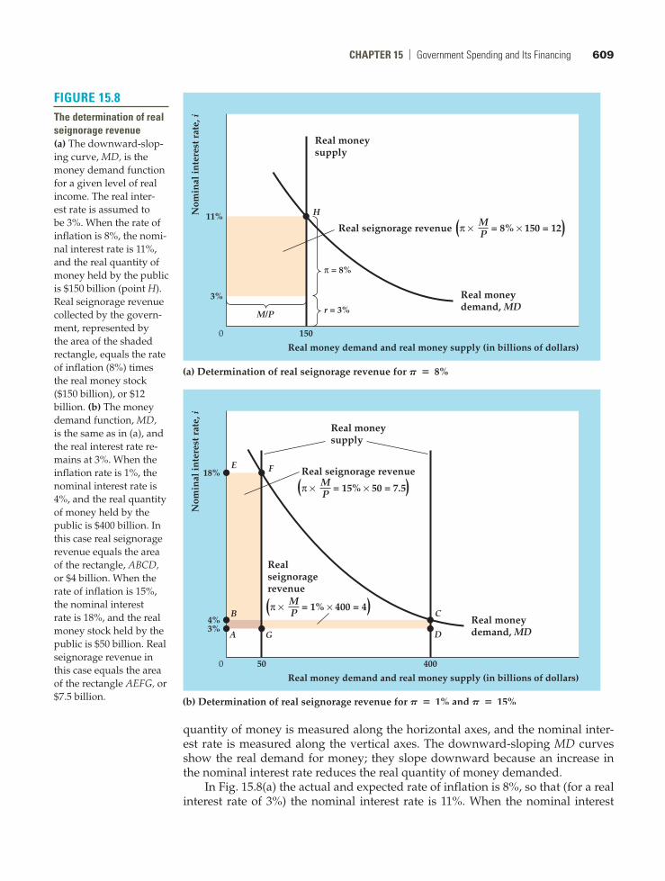
ChapTer 15 | Government Spending and Its Financing 609
quantity of money is measured along the horizontal axes, and the nominal inter-est rate is measured along the vertical axes. The downward-sloping MD curves show the real demand for money; they slope downward because an increase in the nominal interest rate reduces the real quantity of money demanded.
In Fig. 15.8(a) the actual and expected rate of inflation is 8%, so that (for a real interest rate of 3%) the nominal interest rate is 11%. When the nominal interest
FiGure 15.8The determination of real seignorage revenue(a) The downward-slop-ing curve, MD, is the money demand function for a given level of real income. The real inter-est rate is assumed to be 3%. When the rate of inflation is 8%, the nomi-nal interest rate is 11%, and the real quantity of money held by the public is $150 billion (point H). Real seignorage revenue collected by the govern-ment, represented by the area of the shaded rectangle, equals the rate of inflation (8%) times the real money stock ($150 billion), or $12 billion. (b) The money demand function, MD, is the same as in (a), and the real interest rate re-mains at 3%. When the inflation rate is 1%, the nominal interest rate is 4%, and the real quantity of money held by the public is $400 billion. In this case real seignorage revenue equals the area of the rectangle, ABCD, or $4 billion. When the rate of inflation is 15%, the nominal interest rate is 18%, and the real money stock held by the public is $50 billion. Real seignorage revenue in this case equals the area of the rectangle AEFG, or $7.5 billion.
Nom
inal
inte
rest
rat
e, i
Real money demand and real money supply (in billions of dollars)
H
3%
11%
150
Real moneydemand, MD
Real moneysupply
π = 8%
r = 3%M/P
Real seignorage revenue π × = 8% × 150 = 12MP
0
( (
(a) Determination of real seignorage revenue for P ∙ 8%
(b) Determination of real seignorage revenue for P ∙ 1% and P ∙ 15%
Nom
inal
inte
rest
rat
e, i
Real money demand and real money supply (in billions of dollars)
FE
C
D
B
A G
50 400
3%4%
18% Real seignorage revenue
π × = 15% × 50 = 7.5MP
Realseignoragerevenue
π × = 1% × 400 = 4MP
Real moneydemand, MD
Real moneysupply
0
( (
( (
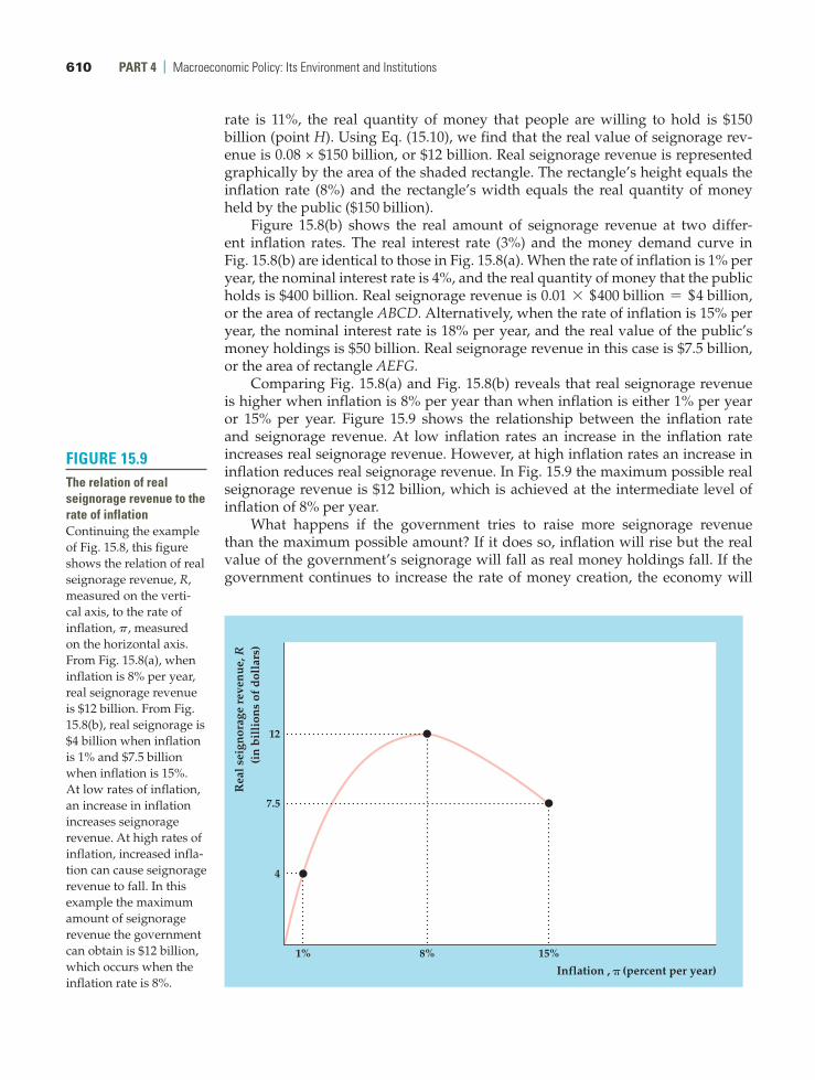
610 parT 4 | Macroeconomic Policy: Its Environment and Institutions
rate is 11%, the real quantity of money that people are willing to hold is $150 billion (point H). Using Eq. (15.10), we find that the real value of seignorage rev-enue is 0.08 × $150 billion, or $12 billion. Real seignorage revenue is represented graphically by the area of the shaded rectangle. The rectangle’s height equals the inflation rate (8%) and the rectangle’s width equals the real quantity of money held by the public ($150 billion).
Figure 15.8(b) shows the real amount of seignorage revenue at two differ-ent inflation rates. The real interest rate (3%) and the money demand curve in Fig. 15.8(b) are identical to those in Fig. 15.8(a). When the rate of inflation is 1% per year, the nominal interest rate is 4%, and the real quantity of money that the public holds is $400 billion. Real seignorage revenue is 0.01 * +400 billion = +4 billion, or the area of rectangle ABCD. Alternatively, when the rate of inflation is 15% per year, the nominal interest rate is 18% per year, and the real value of the public’s money holdings is $50 billion. Real seignorage revenue in this case is $7.5 billion, or the area of rectangle AEFG.
Comparing Fig. 15.8(a) and Fig. 15.8(b) reveals that real seignorage revenue is higher when inflation is 8% per year than when inflation is either 1% per year or 15% per year. Figure 15.9 shows the relationship between the inflation rate and seignorage revenue. At low inflation rates an increase in the inflation rate increases real seignorage revenue. However, at high inflation rates an increase in inflation reduces real seignorage revenue. In Fig. 15.9 the maximum possible real seignorage revenue is $12 billion, which is achieved at the intermediate level of inflation of 8% per year.
What happens if the government tries to raise more seignorage revenue than the maximum possible amount? If it does so, inflation will rise but the real value of the government’s seignorage will fall as real money holdings fall. If the government continues to increase the rate of money creation, the economy will
FiGure 15.9The relation of real seignorage revenue to the rate of inflationContinuing the example of Fig. 15.8, this figure shows the relation of real seignorage revenue, R, measured on the verti-cal axis, to the rate of inflation, p, measured on the horizontal axis. From Fig. 15.8(a), when inflation is 8% per year, real seignorage revenue is $12 billion. From Fig. 15.8(b), real seignorage is $4 billion when inflation is 1% and $7.5 billion when inflation is 15%. At low rates of inflation, an increase in inflation increases seignorage revenue. At high rates of inflation, increased infla-tion can cause seignorage revenue to fall. In this example the maximum amount of seignorage revenue the government can obtain is $12 billion, which occurs when the inflation rate is 8%.
Rea
l sei
gnor
age
reve
nu
e, R
(i
n b
illi
ons
of d
olla
rs)
Inflation , (percent per year)
1% 8% 15%
4
7.5
12
�

ChapTer 15 | Government Spending and Its Financing 611
experience a high rate of inflation or even hyperinflation. Inflation will continue until the government reduces the rate of money creation either by balancing its budget or by finding some other way to finance its deficit.
In some hyperinflations, governments desperate for revenue raise the rate of money creation well above the level that maximizes real seignorage. For example, in the extreme hyperinflation that hit Germany after World War I, rapid money creation drove the rate of inflation to 322% per month. In contrast, in his clas-sic study of the German hyperinflation, Philip Cagan26 of Columbia University calculated that the constant rate of inflation that would have maximized the German government’s real seignorage revenue was “only” 20% per month.
26“The Monetary Dynamics of Hyperinflation,” in Milton Friedman, ed., Studies in the Quantity Theory of Money, Chicago: University of Chicago Press, 1956.
ChapTer SuMMary 1. Government outlays are government purchases of
goods and services, transfers, and net interest. To pay for them, the government collects revenue by four main types of taxes: personal taxes, contribu-tions for social insurance, taxes on production and imports, and corporate taxes.
2. The government budget deficit equals government outlays minus tax revenues and indicates how much the government must borrow during the year. The primary government budget deficit is the total defi-cit less net interest payments. The primary deficit indicates by how much the cost of current programs (measured by current government purchases and transfers) exceeds tax revenues during the year.
3. Fiscal policy affects the economy through its effects on aggregate demand, government capital forma-tion, and incentives.
4. Increases or decreases in government purchases af-fect aggregate demand by changing desired national saving and shifting the IS curve. If Ricardian equiva-lence doesn’t hold, as Keynesians usually argue, changes in taxes also affect desired national saving, the IS curve, and aggregate demand. Automatic sta-bilizers in the government’s budget allow spending to rise or taxes to fall automatically in a recession, which helps cushion the drop in aggregate demand during a recession. The full-employment deficit is what the deficit would be—given current govern-ment spending programs and tax laws—if the econ-omy were at full employment. Because of automatic stabilizers that increase spending and reduce taxes in recessions, the actual deficit rises above the full-employment deficit in recessions.
5. Government capital formation contributes to the productive capacity of the economy. Government
capital formation includes both investment in physi-cal capital (roads, schools) and investment in human capital (education, child nutrition). Official measures of government investment include only investment in physical capital.
6. The average tax rate is the fraction of total income paid in taxes, and the marginal tax rate is the fraction of an additional dollar of income that must be paid in taxes. Changes in average tax rates and changes in marginal tax rates have different effects on economic behavior. For example, an increase in the average tax rate (with no change in the marginal tax rate) increases labor sup-ply, but an increase in the marginal tax rate (with no change in the average tax rate) decreases labor supply.
7. Policymakers must be concerned about the fact that taxes induce distortions, or deviations in economic behavior from that which would have occurred in the absence of taxes. One strategy for minimizing distortions is to hold tax rates approximately con-stant over time (tax rate smoothing), rather than alternating between high and low tax rates.
8. The national debt equals the value of government bonds outstanding. The government budget deficit, expressed in nominal terms, equals the change in the government debt. The behavior of the debt–GDP ratio over time depends on the ratio of the deficit to nominal GDP, the ratio of total debt to nominal GDP, and the growth rate of nominal GDP.
9. Deficits are a burden on future generations if they cause national saving to fall because lower national saving means that the country will have less capital and fewer foreign assets than it would have had otherwise. Ricardian equivalence indicates that a deficit caused by a tax cut won’t affect consumption and therefore won’t affect national saving. In the
612 parT 4 | Macroeconomic Policy: Its Environment and Institutions
Visit www.myeconlab.com to complete these exercises online and get instant feedback. Exercises that update with real-time data are marked with .
Ricardian view, a tax cut doesn’t affect consumption because the increase in consumers’ current income arising from the tax cut is offset by the prospect of increased taxes in the future, leaving consumers no better off. In theory, Ricardian equivalence still holds if the government debt isn’t repaid by the cur-rent generation, provided that people care about the well-being of their descendants and thus choose not to consume more at their descendants’ expense.
10. Ricardian equivalence may not hold—and thus tax cuts may affect national saving—if (1) borrowing constraints prevent some people from consuming as much as they want to; (2) people are shortsighted and don’t take expected future changes in taxes into
account in their planning; (3) people fail to leave be-quests; or (4) taxes aren’t lump-sum. The empirical evidence on Ricardian equivalence is mixed.
11. Deficits are linked to inflation when a government finances its deficits by printing money. The amount of revenue that the government raises by print-ing money is called seignorage. The real value of seignorage equals the inflation rate times the real money supply. Increasing the inflation rate doesn’t always increase the government’s real seignorage because higher inflation causes the public to hold a smaller real quantity of money. Attempts to push the collection of seignorage above its maximum can lead to hyperinflation.
Key TerMSautomatic stabilizers, p. 589average tax rate, p. 591distortions, p. 592full-employment deficit, p. 589government capital, p. 590
government debt, p. 595inflation tax, p. 608marginal tax rate, p. 591primary government budget
deficit, p. 586
seignorage, p. 606supply-side economics, p. 593tax rate smoothing, p. 594
∆B = nominal government budget deficit (15.3)
The change in the nominal value of the government debt equals the nominal government budget deficit.
change indebt@GDP ratio
=deficit
nominal GDP (15.4)
- a total debt
nominal GDP*
growth rate ofnominal GDP
b
The change in the ratio of government debt outstanding to GDP depends on the ratio of the deficit to nominal GDP, the ratio of total debt to nominal GDP, and the growth rate of nominal GDP.
deficit = ∆B = ∆Bp + ∆Bcb = ∆Bp + ∆M (15.7)
Key equaTiONSThe government budget deficit equals the increase in the stock of government debt outstanding, B, which in turn equals the sum of additional holdings of government debt by the public, Bp, and by the central bank, Bcb. The increase in debt held by the central bank equals the increase in the monetary base, which in an all-currency economy is the same as the increase in the money supply, M.
R =∆M
P = p
MP
. (15.10)
In an all-currency economy, real seignorage revenue, R, equals the increase in the money supply, ∆M, divided by the price level, P. This ratio in turn equals the inflation rate (the tax rate on money) multiplied by the real money supply (the tax base).
reView queSTiONS
1. What are the major components of government out-lays? What are the major sources of government revenues? How does the composition of the Federal government’s outlays and revenues differ from that of state and local governments?
2. Explain the difference between the overall govern-ment budget deficit, the current deficit, and the pri-mary current deficit. Why are three deficit concepts needed?