gpr propagation simulation and fat dipole antenna...

GPR Propagation Simulation and FatDipole Antenna Design

Tai-Lin Greg Chen

A dissertation submitted to the Department of Electrical Engineering,

University of Cape Town, in fulfilment of the requirements

for the degree of Master of Science in Engineering.

Cape Town, March 2006

Declaration

I declare that this dissertation is my own, unaided work. It is being submitted for the

degree of Master of Science in Engineering in the Universityof Cape Town. It has not

been submitted before for any degree or examination in any other university.

Signature of Author . . . . . . . . . . . . . . . . . . . . . . . . . . . . . . . . . .. . . . . . . . . . . . . . . . . . . . . . . . . . . .

Cape Town

February 2006

i

Abstract

Two applications of FEKO are reported. The first applicationis investigating how antennas

propagate, reflect, and the difference in transmit and receive signals in various ground

media. Results of the ground penetration simulations done in FEKO (MoM- Method of

Moment) is compared to Finite Difference Time Domain (FDTD)results simulated by

Mukhopadhyay with the same physical model.

The second application is to model and fabricate an ultra wide-band antenna with implemen-

tation of the fat dipole design. The design considerations applied to improve antenna

performance include antenna feed configurations, substrate width, aperture dimension,

cavity implementation, terminating resistance, antenna impedance and balun matching.

After the design process was completed, fabrication of the antenna took place and the

design validated.

ii

Acknowledgements

I would like to thank my supervisor, Prof. Mike Inggs for his guidance, encouragement

and motivation throughout the entire research period. Special thanks goes to my family

and friends whose continuous support was invaluable to the completion of this project.

I would also like to thank EM Software & Systems for the FEKO licences provided to me,

as well as Pradip Mukhopadhyay, Dr. Richard Lord, the RRSG staff and all my colleagues

in the RRSG for their contribution towards the research.

iii

Contents

Declaration i

Abstract ii

Acknowledgements iii

List of Symbols x

Nomenclature xi

1 Introduction 1

1.1 Project Background . . . . . . . . . . . . . . . . . . . . . . . . . . . . . 1

1.2 Ground Penetrating Radar . . . . . . . . . . . . . . . . . . . . . . . . . 1

1.3 GPR Antenna Requirements . . . . . . . . . . . . . . . . . . . . . . . . 2

1.4 Project Objectives . . . . . . . . . . . . . . . . . . . . . . . . . . . . . . 3

1.5 Plan of Development . . . . . . . . . . . . . . . . . . . . . . . . . . . . 4

2 Background Technology 7

2.1 Method of Moment (MoM) . . . . . . . . . . . . . . . . . . . . . . . . . 7

2.2 Finite-Difference Time Domain (FDTD) . . . . . . . . . . . . . . .. . . 7

2.3 Window Functions . . . . . . . . . . . . . . . . . . . . . . . . . . . . . 8

2.4 Ground Penetrating Radar . . . . . . . . . . . . . . . . . . . . . . . . . 8

2.5 GPR Antenna . . . . . . . . . . . . . . . . . . . . . . . . . . . . . . . . 9

2.6 Ultra Wide-Band (UWB) . . . . . . . . . . . . . . . . . . . . . . . . . . 9

2.7 Reflection Coefficient . . . . . . . . . . . . . . . . . . . . . . . . . . . 10

2.8 Voltage Standing Wave Ratio (VSWR) . . . . . . . . . . . . . . . . . .. 10

iv

2.9 Radiation Pattern . . . . . . . . . . . . . . . . . . . . . . . . . . . . . . 11

2.10 Radiation Efficiency . . . . . . . . . . . . . . . . . . . . . . . . . . . . 11

2.11 Antenna Gain . . . . . . . . . . . . . . . . . . . . . . . . . . . . . . . . 12

2.12 Termination Resistor . . . . . . . . . . . . . . . . . . . . . . . . . . . .12

2.13 Cross-Coupling . . . . . . . . . . . . . . . . . . . . . . . . . . . . . . . 13

2.14 Conclusion . . . . . . . . . . . . . . . . . . . . . . . . . . . . . . . . . 13

3 Ground Penetration Transmitter-Receiver Time Response Simulations 14

3.1 Simulation Configuration . . . . . . . . . . . . . . . . . . . . . . . . . .14

3.2 Excitation . . . . . . . . . . . . . . . . . . . . . . . . . . . . . . . . . . 16

3.3 Results . . . . . . . . . . . . . . . . . . . . . . . . . . . . . . . . . . . . 17

3.4 Conclusion . . . . . . . . . . . . . . . . . . . . . . . . . . . . . . . . . 21

4 Fat Dipole Modelling 22

4.1 Modelling of UWB Fat Dipole Antenna . . . . . . . . . . . . . . . . . .22

4.2 Modelling of 400 - 800MHz Fat Dipole . . . . . . . . . . . . . . . . . .26

4.3 Modelling of Cased Fat Dipole with Edge Terminating Resistors . . . . . 30

4.4 Conclusion . . . . . . . . . . . . . . . . . . . . . . . . . . . . . . . . . 37

5 Antenna Construction and Verification 39

5.1 Antenna Aperture and Casing Construction . . . . . . . . . . . .. . . . 39

5.2 Balun Feed . . . . . . . . . . . . . . . . . . . . . . . . . . . . . . . . . 39

5.3 Terminating Resistors . . . . . . . . . . . . . . . . . . . . . . . . . . . .40

5.4 Return Loss Measurement . . . . . . . . . . . . . . . . . . . . . . . . . 41

5.5 Coupling Analysis . . . . . . . . . . . . . . . . . . . . . . . . . . . . . 43

5.6 Object Detection . . . . . . . . . . . . . . . . . . . . . . . . . . . . . . 46

5.7 Conclusion . . . . . . . . . . . . . . . . . . . . . . . . . . . . . . . . . 47

6 Conclusions and Recommendations 49

6.1 Ground penetration transmitter-receiver time response simulations done

in FEKO and FDTD . . . . . . . . . . . . . . . . . . . . . . . . . . . . . 49

6.2 GPR fat dipole modelling . . . . . . . . . . . . . . . . . . . . . . . . . . 49

6.3 Future work . . . . . . . . . . . . . . . . . . . . . . . . . . . . . . . . . 50

v

A Software Source Code 51

A.1 FEKO Code . . . . . . . . . . . . . . . . . . . . . . . . . . . . . . . . . 51

A.1.1 Subsurface Transit Response - EDITFEKO . . . . . . . . . . . .51

A.1.2 Subsurface Transit Response - TIMEFEKO . . . . . . . . . . . .55

A.1.3 KERI and Microline Co. Ltd Fat Dipole - EDITFEKO . . . . . .55

A.1.4 Improved 400 - 800 MHz Fat Dipole - EDITFEKO . . . . . . . . 57

A.2 IDL Code . . . . . . . . . . . . . . . . . . . . . . . . . . . . . . . . . . 58

A.2.1 Subsurface Time Response - Graphical Display . . . . . . .. . . 58

A.2.2 Object Detection . . . . . . . . . . . . . . . . . . . . . . . . . . 61

B TC4-1W Balun Transformer Data Sheet 65

vi

List of Figures

1.1 Subsurface media simulation configuration . . . . . . . . . . .. . . . . . 4

1.2 Fat dipole ultra wide-band antenna model (3D gain). . . . .. . . . . . . 5

2.1 Common window functions[4] . . . . . . . . . . . . . . . . . . . . . . . 8

2.2 UWB definition[2] . . . . . . . . . . . . . . . . . . . . . . . . . . . . . 10

2.3 GPR directivity . . . . . . . . . . . . . . . . . . . . . . . . . . . . . . . 11

2.4 Illustration of cross-coupling and clutter of signals .. . . . . . . . . . . 13

3.1 Dimensions of the layered media under investigation. . .. . . . . . . . . 15

3.2 Subsurface simulation 3D model in FEKO . . . . . . . . . . . . . . .. . 16

3.3 Transmitted pulse and its spectral representation. . . .. . . . . . . . . . 17

3.4 Received waveforms obtained using FEKO. . . . . . . . . . . . . .. . . 19

3.5 Received waveforms obtained by K.P. Mukhopadhyay usingFDTD.[7] . . 20

3.6 Over-plot of FEKO and FDTD receiver waveforms. . . . . . . . .. . . 21

4.1 Picture of KERI and Microline fat dipole[14] . . . . . . . . . .. . . . . 23

4.2 100 - 400MHz fat dipole VSWR[14] . . . . . . . . . . . . . . . . . . . . 23

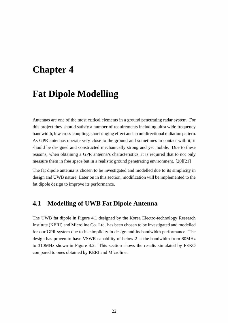
4.3 KERI and Microline fat dipole in FEKO . . . . . . . . . . . . . . . . .. 24

4.4 Fat dipole model with wired feed segment structure . . . . .. . . . . . . 24

4.5 Fat dipole model with edge feed structure . . . . . . . . . . . . .. . . . 25

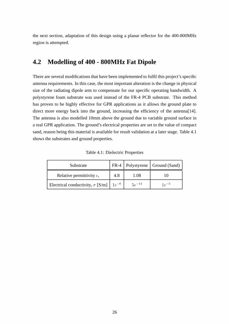
4.6 KERI and Microline fat dipole VSWR using FEKO . . . . . . . . . .. . 25

4.7 FEKO model of 400 - 800MHz fat dipole . . . . . . . . . . . . . . . . . 27

4.8 S11 of various fat dipole substrate heights . . . . . . . . . . .. . . . . . 28

4.9 Power radiated . . . . . . . . . . . . . . . . . . . . . . . . . . . . . . . 28

4.10 Electric near field indicating amount of power radiating vertically into the

ground . . . . . . . . . . . . . . . . . . . . . . . . . . . . . . . . . . . . 29

vii

4.11 Fat dipole radiation pattern at 600MHz . . . . . . . . . . . . . .. . . . . 30

4.12 Front view of the simulated antenna model . . . . . . . . . . . .. . . . . 31

4.13 Side view of the simulated antenna model . . . . . . . . . . . . .. . . . 31

4.14 Top view of the simulated antenna model . . . . . . . . . . . . . .. . . 32

4.15 Impedance and S11 simulated result before implementing terminating

resistors . . . . . . . . . . . . . . . . . . . . . . . . . . . . . . . . . . . 33

4.16 Edge termination resistor connections . . . . . . . . . . . . .. . . . . . 34

4.17 Improved S11 and near field result (at 600MHz) after implementing termination

resistors . . . . . . . . . . . . . . . . . . . . . . . . . . . . . . . . . . . 35

4.18 3D radiation gain pattern indication the directivity of the cased fat dipole . 36

4.19 Radiation efficiency of the final antenna model . . . . . . . .. . . . . . 37

5.1 Balun architecture and antenna feed structure . . . . . . . .. . . . . . . 40

5.2 Picture of TC4-1W RF Transformer[Appendix B] . . . . . . . . .. . . . 40

5.3 Photograph of the antennas and S11 sand box testing arrangement with

Agilent E5062A network analyser . . . . . . . . . . . . . . . . . . . . . 42

5.4 Validating the fabricated antenna S11 with the simulated result . . . . . . 43

5.5 Bistatic antenna configurations . . . . . . . . . . . . . . . . . . . .. . . 44

5.6 Cross-coupling of antennas at 0mm separation . . . . . . . . .. . . . . . 44

5.7 Cross-coupling of antennas at 5mm separation . . . . . . . . .. . . . . . 45

5.8 Cross-coupling of antennas at 10mm separation . . . . . . . .. . . . . . 45

5.9 Cross-coupling of antenna at 15mm separation . . . . . . . . .. . . . . . 45

5.10 Sand box object detection test configuration . . . . . . . . .. . . . . . . 46

5.11 Time-domain object detection results of a metal plate buried at a depth of

15cm . . . . . . . . . . . . . . . . . . . . . . . . . . . . . . . . . . . . 47

viii

List of Tables

3.1 Electrical properties of sand and clay used in computation. . . . . . . . . 15

3.2 Calculated time response . . . . . . . . . . . . . . . . . . . . . . . . . .18

4.1 Dielectric Properties . . . . . . . . . . . . . . . . . . . . . . . . . . . .26

4.2 Cased fat dipole Antenna simulation dimension in mm . . . .. . . . . . 32

ix

List of Symbols

σ — Electrical conductivity

ǫr — Relative dielectric permittivity

c — Speed of light

µr — Relative dielectric permeability

fb — Operating bandwidth

fc — Centre frequency

fL — Bandwidth starting frequency

fH — Bandwidth ending frequency

Γ — Voltage reflective coefficient

ZL — Load Impedance

Zo — Antenna Characteristic Impedance

η — Radiation efficiency

Gd — Directive Gain

Gp — Power Gain

Pmax — Maximum power density

Pt — Total power radiated

Po — Total power accepted

λ — Wavelength

S11 — Return loss

S12 — Insertion loss

x

Nomenclature

Co-polarization—The polarisation which the antenna is intended to radiate.

Cross-polarization—The polarization orthogonal to a specific reference polarization.

MoM —Method of Moment.

FDTD—Finite Difference Time Domain.

GPR—Ground penetrating radar.

UWB—Ultra wide-band.

NB—Narrow band

KERI —Korea Electro-technology Research Institute

VSWR—Voltage standing wave ratio.

EM—Electromagnetic.

FFT—Fast Fourier transform.

Tx—Transmitter.

Rx—Receiver.

xi

Chapter 1

Introduction

1.1 Project Background

FEKO is a full wave, MoM (method of moment) based simulation software for the analysis

of electromagnetic problems such as coupling, antenna design, antenna placement analysis,

microstrip design, scattering analysis, etc. It has the ability to solve electrically large

problems using accurate full wave techniques. Electromagnetic fields are obtained by first

calculating the electric surface currents on conducting surfaces and equivalent electric and

magnetic surface current on the surface of a dielectric solid. The currents are calculated

using a linear combination of basis functions, where the coefficients are obtained by

solving a system of linear equations. Once the current distribution is known, further

parameters can be obtained, such as near field, far field, directivity, input impedance of an

antenna and importantly, radar cross sections[6].

RRSG (Radar and Remote Sensing Group) at UCT sees this as an opportunity to use

FEKO as a modelling tool used in investigating subsurface transmitter-receiver wave

response and the design of an ultra wide-band ground penetrating antenna.

1.2 Ground Penetrating Radar

Ground penetrating radar (GPR) is a surveying tool that is used to read cross-sectional

subsurface information without physically probing or changing the physical form of the

medium under investigation. Its main functions are to evaluate the location and depth of

subsurface objects and to investigate their presence.

GPR operates by transmitting frequency waves directing down into the ground via a wide-

band antenna. When the transmitted signal enters the groundand reaches objects or

1

mediums with different electrical and dielectric properties, part of the signal is reflected

off. This reflected energy is then sensed by the receiver antenna[19].

The following are a list of GPR applications:

• Land mine detection

• Imaging underground caves

• Locating mine tunnels

• Detection of pipes

• Detection of buried debris

• Borehole monostatic, bistatic radar applications

The radar waves can penetrate up to 30 metres[1] depending onthe conductivity of the

ground and the operating frequency of the antenna. The higher the frequency the better

the resolution, but less penetrating depth. The lower the frequency the further the waves

can penetrate, but at poorer resolution. In this project, weare interested in designing GPR

antennas operating in the region of 400 - 800MHz[1].

1.3 GPR Antenna Requirements

The following antenna specifications were required for thisproject as well as general GPR

practice.

1. Operating bandwidth of between 400 - 800MHz, i.e. Ultra wide-bandwidth, bandwidth

greater than 20% of centre frequency.

2. Directive antenna with maximum energy projecting into the ground.

3. Antenna will need to be robust and mobile for active GPR testing.

4. Antenna’s input impedance will have to be balanced and transformed to50Ω to

minimise mismatch between antenna and radar.

2

1.4 Project Objectives

The project had two phases which extensively used FEKO as themain source of development.

The first phase is learning how to use the package for GPR applications (FEKO’s planar

multilayer Green’s function is an effective tool used to simulate multiple layered media for

both antenna design and subsurface detection). First phaseof the project is investigating

how antennas propagate from the transmiter to a receiver in amulti-layered subsurface

environment. The direct and reflected receiver time response signal effected by various

ground media is studied. Results of the ground penetration simulations done in FEKO

(MoM- Method of Moment) is compared to Finite Difference Time Domain (FDTD)

results simulated by Mukhopadhyay with the same physical model. This is shown in

Chapter 3.

The second phase is to model and fabricate an ultra wide-bandantenna with implementation

of the fat dipole design. The results shown in Chapter 4 indicate design considerations

applied to improve antenna performance include antenna feed configurations, substrate

width, aperture dimension, terminating resistance, antenna impedance and balun matching.

After the design process was completed, fabrication of the antenna took place and necessary

results were obtained to validate the design.

The project objectives are thus listed below:

1. To familiarise using FEKO and understand the FEKO simulation package in the

GPR antenna design and application aspects.

2. To create and simulate the subsurface media models investigated by K.P. Mukhopadhyay

using FDTD method in FEKO.

3. Compare the time-domain MoM results with the existing FDTD results.

4. To review the UWB GPR antennas fat dipole antenna design under consideration

and simulate for result consistency.

5. Use FEKO to model and improve performance and characteristic of the antenna to

meet GPR specifications.

6. To fabricate the antenna and make measurements to validate design.

7. To draw conclusions and make recommendations about the research done in both

subsurface media investigation and UWB fat dipole antenna.

3

1.5 Plan of Development

Chapter 2 reviews the background technologies that are usedthis in project so far. Simulation

methods are explained in this chapter include MoM, Green’s function, FDTD and window

functions. Antenna definitions such as UWB, reflection coefficient, VSWR, radiation

patterns, termination resistance and antenna coupling arealso briefly explained.

In Chapter 3, FEKO is used to compare results of transmitter-receiver time response

obtained from a finite difference time domain (FDTD) method simulator with those calculated

with FEKO. A transmitter and receiver antenna are positioned a set of distances apart

situated in a subsurface layered media (sand and clay), timeresponse of the direct and

reflected EM waves propagating through the media, and the comparison in shape difference

of waveforms obtained between point source (Blackman-Harris window function) and

simulated dipole antennas are investigated. [Figure 1.1]

Figure 1.1: Subsurface media simulation configuration

In Chapter 4, a 100-400MHz UWB fat dipole antenna designed byKorea Electro-technology

Research Institute (KERI) and Microline Co. Ltd. is reviewed. This design implements

the wide-band characteristics of an extended width patch dipole for GPR applications.

FEKO is used to model this antenna design and compare the simulated results with the

original developer’s VSWR (voltage standing wave ratio). The result from this experiment

validate the feasibility of modelling such design in FEKO for this project.

After validation of the fat dipole design, several 400-800MHz dipoles were simulated with

different dielectric (polystyrene foam) and substrate height to investigate how it effects the

4

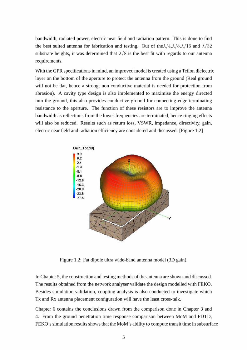
bandwidth, radiated power, electric near field and radiation pattern. This is done to find

the best suited antenna for fabrication and testing. Out of theλ/4,λ/8,λ/16 andλ/32

substrate heights, it was determined thatλ/8 is the best fit with regards to our antenna

requirements.

With the GPR specifications in mind, an improved model is created using a Teflon dielectric

layer on the bottom of the aperture to protect the antenna from the ground (Real ground

will not be flat, hence a strong, non-conductive material is needed for protection from

abrasion). A cavity type design is also implemented to maximise the energy directed

into the ground, this also provides conductive ground for connecting edge terminating

resistance to the aperture. The function of these resistorsare to improve the antenna

bandwidth as reflections from the lower frequencies are terminated, hence ringing effects

will also be reduced. Results such as return loss, VSWR, impedance, directivity, gain,

electric near field and radiation efficiency are considered and discussed. [Figure 1.2]

Figure 1.2: Fat dipole ultra wide-band antenna model (3D gain).

In Chapter 5, the construction and testing methods of the antenna are shown and discussed.

The results obtained from the network analyser validate thedesign modelled with FEKO.

Besides simulation validation, coupling analysis is also conducted to investigate which

Tx and Rx antenna placement configuration will have the leastcross-talk.

Chapter 6 contains the conclusions drawn from the comparison done in Chapter 3 and

4. From the ground penetration time response comparison between MoM and FDTD,

FEKO’s simulation results shows that the MoM’s ability to compute transit time in subsurface

5

layered media has a comparable accuracy to one using FDTD method. FEKO’s planar

multilayer Green’s function has proven to be a useful tool for dielectric antenna modelling,

with relatively comparable result with the ones obtained bythe network analyser. The

modification of implementing an expanded polystyrene filledmetal cavity and termination

resistors has improved the performance of the system considerably, mainly with regards

to radiation efficiency and bandwidth.

6

Chapter 2

Background Technology

This chapter contains basic definitions of the technologiesimplemented so far in this

project. It will go through the mathematical models used by the EM simulators, and

antenna theories involved in this report.

2.1 Method of Moment (MoM)

This is a technique to construct estimators of the parameters that is based on matching the

sample moment with the corresponding distribution moments. The fundamental concept

behind the MoM is implementing orthogonal expansions and linear algebra to reduce

the integral equation problem to a system of simultaneous linear equations. This is

achieved by defining the unknown current distribution in terms of an othogonal set of

basis functions and defining the boundary conditions[15]. Applying this definition to

antenna modelling, it means that the method of moment startsby deriving the current on

each segment, or the strength of each moment, by using a coupling Green’s function.

Green’s functions incorporates electrostatic coupling between the moments for if the

spatial charge of the currents is known accurately then one can compute the build up

of charges at points on the structure. Once the current distribution is known, parameters

then can be obtained[6][15].

2.2 Finite-Difference Time Domain (FDTD)

FDTD is a full-wave, dynamic and powerful tool to solve Maxwell’s equations. This

method belongs in the general class of differential time domain numerical modeling

methods. Maxwell’s equation are modified to central-difference equations and implemented

in software. These equations are solved by solving the electric field at a given instant in

7

time, then the magnetic field are solved at the next instant intime, and the process repeat

itself untill the model is resolved.

FDTD is a useful numerical method suitable for modelling EM wave propagation trough

complex media. Furthermore, it is ideal for modelling transient EM fields in inhomogeneous

media, such as complex geographical structures as it fit relatively into the finite-difference

grid, and absorbing boundary conditions can truncated the grid to simulate an infinite

region [8].

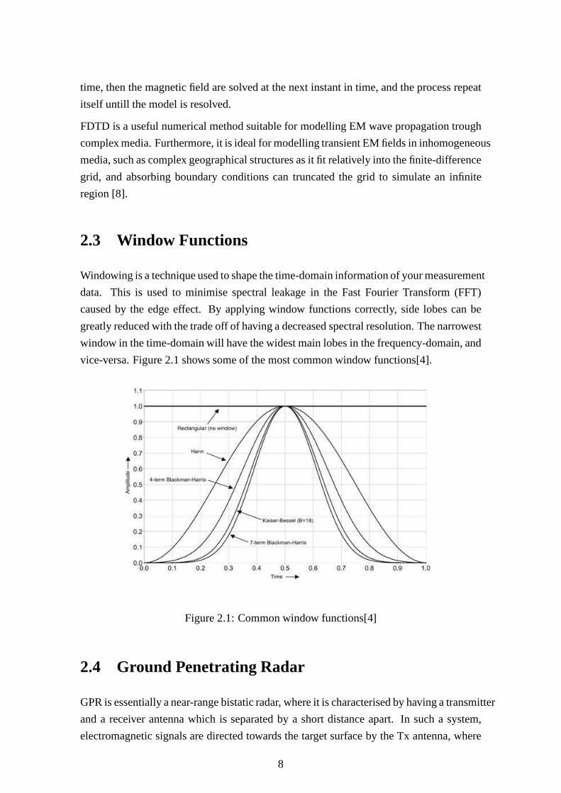
2.3 Window Functions

Windowing is a technique used to shape the time-domain information of your measurement

data. This is used to minimise spectral leakage in the Fast Fourier Transform (FFT)

caused by the edge effect. By applying window functions correctly, side lobes can be

greatly reduced with the trade off of having a decreased spectral resolution. The narrowest

window in the time-domain will have the widest main lobes in the frequency-domain, and

vice-versa. Figure 2.1 shows some of the most common window functions[4].

Figure 2.1: Common window functions[4]

2.4 Ground Penetrating Radar

GPR is essentially a near-range bistatic radar, where it is characterised by having a transmitter

and a receiver antenna which is separated by a short distanceapart. In such a system,

electromagnetic signals are directed towards the target surface by the Tx antenna, where

8

the signals will partially reflect back towards the antenna,but more importantly, the main

portion of the signal will penetrate the surface and is then scattered by any contrast in

subsurface material. This scattered signal is then propagated back to the Rx antenna.

There also exists a monostatic GPR arrangement where a single antenna is responsible

for both transmitting and receiving, but in this project only the bistatic method will be

investigated for antenna design[21].

2.5 GPR Antenna

“It is believed that the main breakthrough in GPR hardware can be achieved in the antenna

design”[20]. Antennas are one of the most critical elementsin a ground penetrating radar

system. They should satisfy a number of requirement but the most important one is

the wide frequency band. Due to the fact that GPR is essentially a near-range radar,

its antenna elements should possess low coupling between the transmitter and receiver,

both should also have short ringing effect.

As GPR antennas operate very close to the ground and sometimes in contact with it,

the changes in ground properties, which includes the types of ground medium and its

elevation, this should not strongly affect the antennas performance. Hence when obtaining

a GPR antenna’s characteristics one should not only measurethem in free space but in a

realistic ground penetrating environment[21].

2.6 Ultra Wide-Band (UWB)

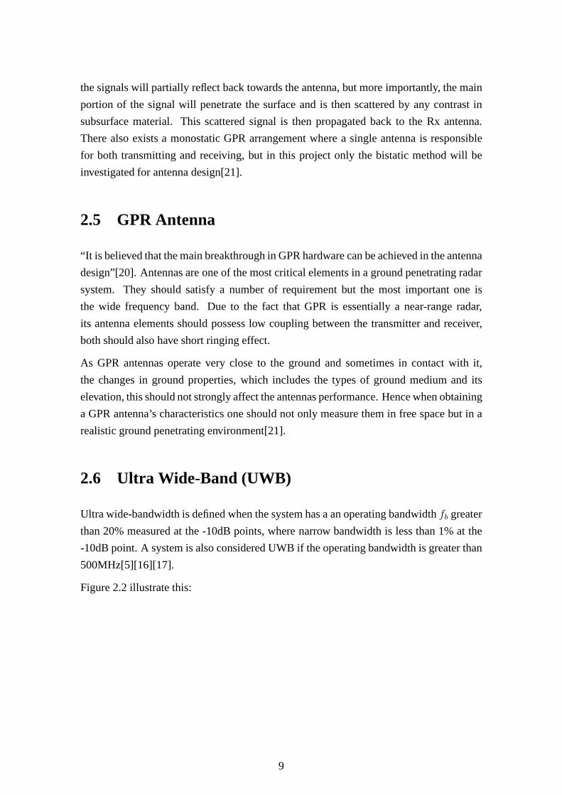
Ultra wide-bandwidth is defined when the system has a an operating bandwidthfb greater

than 20% measured at the -10dB points, where narrow bandwidth is less than 1% at the

-10dB point. A system is also considered UWB if the operatingbandwidth is greater than

500MHz[5][16][17].

Figure 2.2 illustrate this:

9

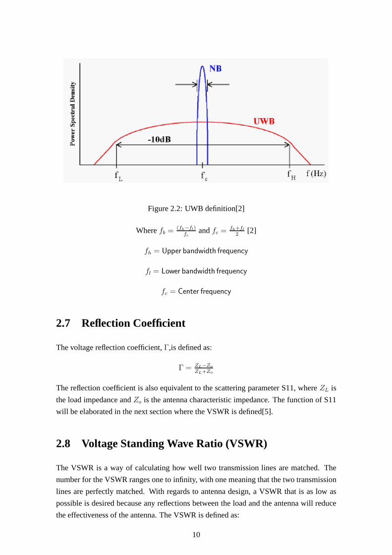
Figure 2.2: UWB definition[2]

Wherefb =(fh−fl)

fcandfc =

fh+fl

2[2]

fh = Upper bandwidth frequency

fl = Lower bandwidth frequency

fc = Center frequency

2.7 Reflection Coefficient

The voltage reflection coefficient,Γ,is defined as:

Γ =ZL−Zo

ZL+Zo

The reflection coefficient is also equivalent to the scattering parameter S11, whereZL is

the load impedance andZo is the antenna characteristic impedance. The function of S11

will be elaborated in the next section where the VSWR is defined[5].

2.8 Voltage Standing Wave Ratio (VSWR)

The VSWR is a way of calculating how well two transmission lines are matched. The

number for the VSWR ranges one to infinity, with one meaning that the two transmission

lines are perfectly matched. With regards to antenna design, a VSWR that is as low as

possible is desired because any reflections between the loadand the antenna will reduce

the effectiveness of the antenna. The VSWR is defined as:

10

V SWR =1+Γ1−Γ

WhereΓ is defined previously as the reflection coefficient[5].

2.9 Radiation Pattern

The radiation pattern indicates how directionally the antenna is radiating power, this is

measured as the 3 dimensional far-field spread around the antenna. The radiation pattern

required for GPR applications must be unidirectional, thismeans that power radiated

must be more focused at a narrow angular direction rather than spread evenly around

the antenna. The need for this characteristic is to eliminate ambiguous target detection.

Figure 2.3 illustrates this.

Figure 2.3: GPR directivity

2.10 Radiation Efficiency

The radiation efficiencyη of an antenna is the ratio of the total power radiated by an

antenna to the net power accepted by the antenna at its input terminals during the radiation

process[22]. Where:

11

η =Pr

Pa

WherePr = Total radiated power

Pa = Net power accepted

2.11 Antenna Gain

There are two different types of antenna gain, being the directive gain and the power

gain. The directive gain is referred to as the directivity and the power gain simply as

gain. The directivity is defined as the radiation intensity in a directionθ relative to the

average intensity of an isotropic radiator. This can also beexpressed in terms of the

maximum radiated-power density at a far-field distanceR relative to the average density

if an isotropic radiator atR [23]:

Gd =Pmax

Pt/4πR2

WherePmax = Maximum power radiated

andPt = Total power radiated

The power gain or gainGpof the antenna referred to an isotropic source is the ratio of

its maximum radiation intensity to the intensity of a lossless isotropic source with equal

power input[23]:

Gp =Pmax

Po/4πR2

WherePo = Total power accepted

2.12 Termination Resistor

The purpose of a termination resistor is to minimise unwanted reflections on a transmission

line and hence assuring maximum signal integrity. Applyingthis component to the edge

of an aperture, it becomes an impedance termination resistor and increases the bandwidth

of the antenna as low frequency reflections from the edges areabsorbed. For a GPR

application, the termination resistance also reduces the ringing effect from buried object.

The effectiveness of the termination will depend on how closely the resistance value

matches the feed point impedance of the antenna, but it has been shown that a slightly

higher resistance value compared to the impedance gives an optimal effect. [10, 11, 12,

14]

12

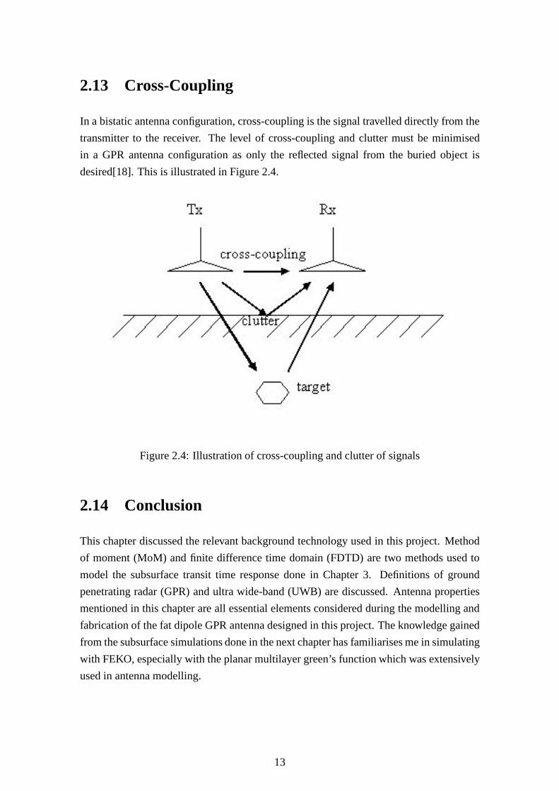
2.13 Cross-Coupling

In a bistatic antenna configuration, cross-coupling is the signal travelled directly from the

transmitter to the receiver. The level of cross-coupling and clutter must be minimised

in a GPR antenna configuration as only the reflected signal from the buried object is

desired[18]. This is illustrated in Figure 2.4.

Figure 2.4: Illustration of cross-coupling and clutter of signals

2.14 Conclusion

This chapter discussed the relevant background technologyused in this project. Method

of moment (MoM) and finite difference time domain (FDTD) are two methods used to

model the subsurface transit time response done in Chapter 3. Definitions of ground

penetrating radar (GPR) and ultra wide-band (UWB) are discussed. Antenna properties

mentioned in this chapter are all essential elements considered during the modelling and

fabrication of the fat dipole GPR antenna designed in this project. The knowledge gained

from the subsurface simulations done in the next chapter hasfamiliarises me in simulating

with FEKO, especially with the planar multilayer green’s function which was extensively

used in antenna modelling.

13

Chapter 3

Ground Penetration

Transmitter-Receiver Time Response

Simulations

The applications of ground penetrating radar has being hugely increased to gain valuable

information such as water content of soil, depth of water, buried objects and void detection

[7]. In this chapter, a study conducted by K.P. Mudhopadhyay(2004) investigating the EM

waves propagating through layered media simulated using FDTD method will be shown,

and compared to results obtained using FEKO, a frequency based MoM code.

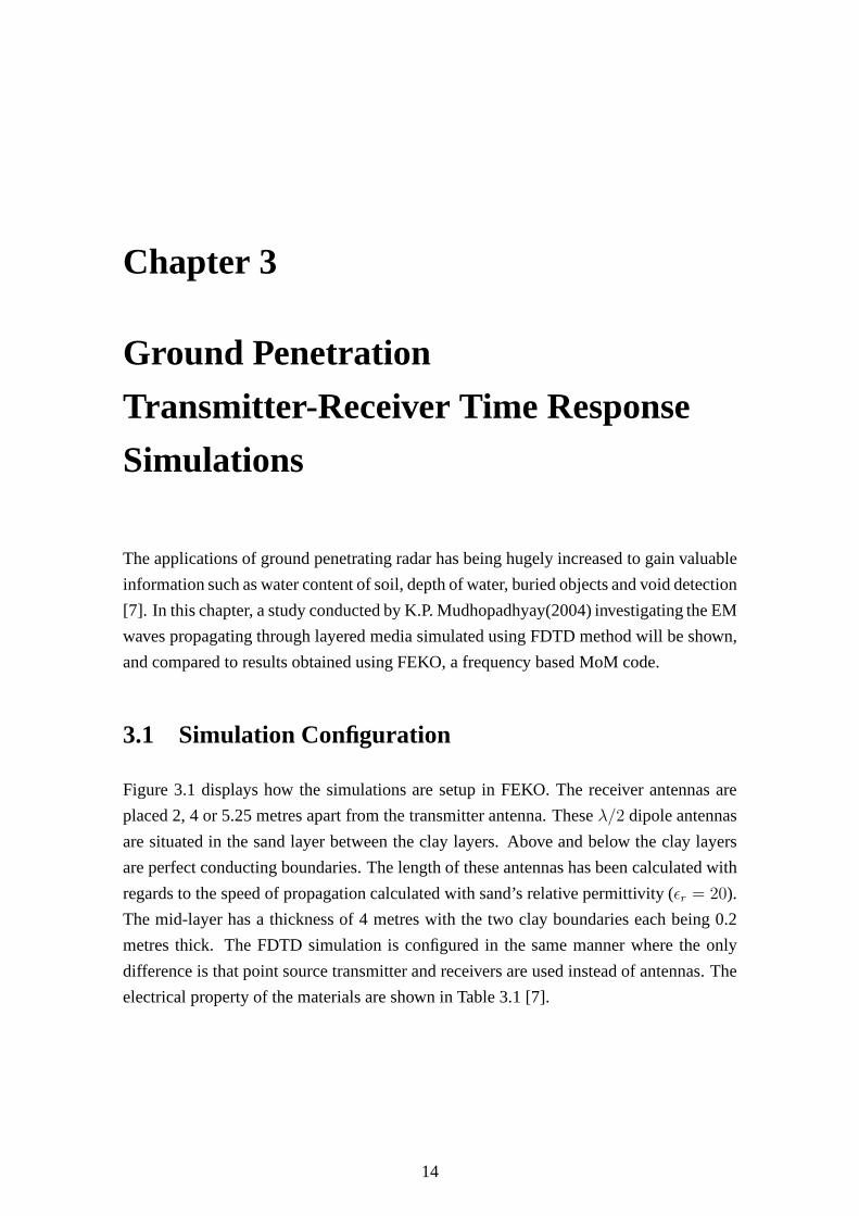
3.1 Simulation Configuration

Figure 3.1 displays how the simulations are setup in FEKO. The receiver antennas are

placed 2, 4 or 5.25 metres apart from the transmitter antenna. Theseλ/2 dipole antennas

are situated in the sand layer between the clay layers. Aboveand below the clay layers

are perfect conducting boundaries. The length of these antennas has been calculated with

regards to the speed of propagation calculated with sand’s relative permittivity (ǫr = 20).

The mid-layer has a thickness of 4 metres with the two clay boundaries each being 0.2

metres thick. The FDTD simulation is configured in the same manner where the only

difference is that point source transmitter and receivers are used instead of antennas. The

electrical property of the materials are shown in Table 3.1 [7].

14

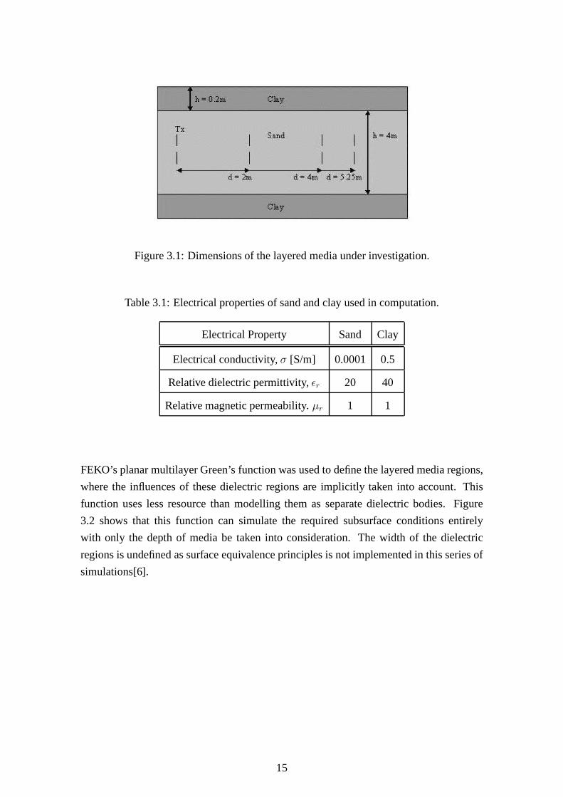
Figure 3.1: Dimensions of the layered media under investigation.

Table 3.1: Electrical properties of sand and clay used in computation.

Electrical Property Sand Clay

Electrical conductivity,σ [S/m] 0.0001 0.5

Relative dielectric permittivity,ǫr 20 40

Relative magnetic permeability.µr 1 1

FEKO’s planar multilayer Green’s function was used to definethe layered media regions,

where the influences of these dielectric regions are implicitly taken into account. This

function uses less resource than modelling them as separatedielectric bodies. Figure

3.2 shows that this function can simulate the required subsurface conditions entirely

with only the depth of media be taken into consideration. Thewidth of the dielectric

regions is undefined as surface equivalence principles is not implemented in this series of

simulations[6].

15

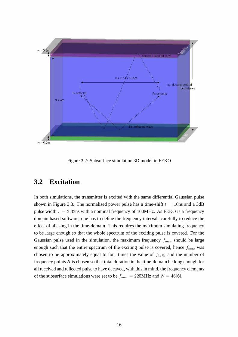
Figure 3.2: Subsurface simulation 3D model in FEKO

3.2 Excitation

In both simulations, the transmitter is excited with the same differential Gaussian pulse

shown in Figure 3.3. The normalised power pulse has a time-shift t = 10ns and a 3dB

pulse widthτ = 3.33ns with a nominal frequency of 100MHz. As FEKO is a frequency

domain based software, one has to define the frequency intervals carefully to reduce the

effect of aliasing in the time-domain. This requires the maximum simulating frequency

to be large enough so that the whole spectrum of the exciting pulse is covered. For the

Gaussian pulse used in the simulation, the maximum frequency fmax should be large

enough such that the entire spectrum of the exciting pulse iscovered, hencefmax was

chosen to be approximately equal to four times the value off3dB, and the number of

frequency pointsN is chosen so that total duration in the time-domain be long enough for

all received and reflected pulse to have decayed, with this inmind, the frequency elements

of the subsurface simulations were set to befmax = 225MHz andN = 46[6].

16

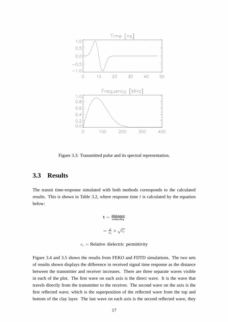
Figure 3.3: Transmitted pulse and its spectral representation.

3.3 Results

The transit time-response simulated with both methods corresponds to the calculated

results. This is shown in Table 3.2, where response timet is calculated by the equation

below:

t =distancevelocity

=dc0×√

ǫr

ǫr = Relative dielectric permittivity

Figure 3.4 and 3.5 shows the results from FEKO and FDTD simulations. The two sets

of results shown displays the difference in received signaltime response as the distance

between the transmitter and receiver increases. There are three separate waves visible

in each of the plot. The first wave on each axis is the direct wave. It is the wave that

travels directly from the transmitter to the receiver. The second wave on the axis is the

first reflected wave, which is the superposition of the reflected wave from the top and

bottom of the clay layer. The last wave on each axis is the second reflected wave, they

17

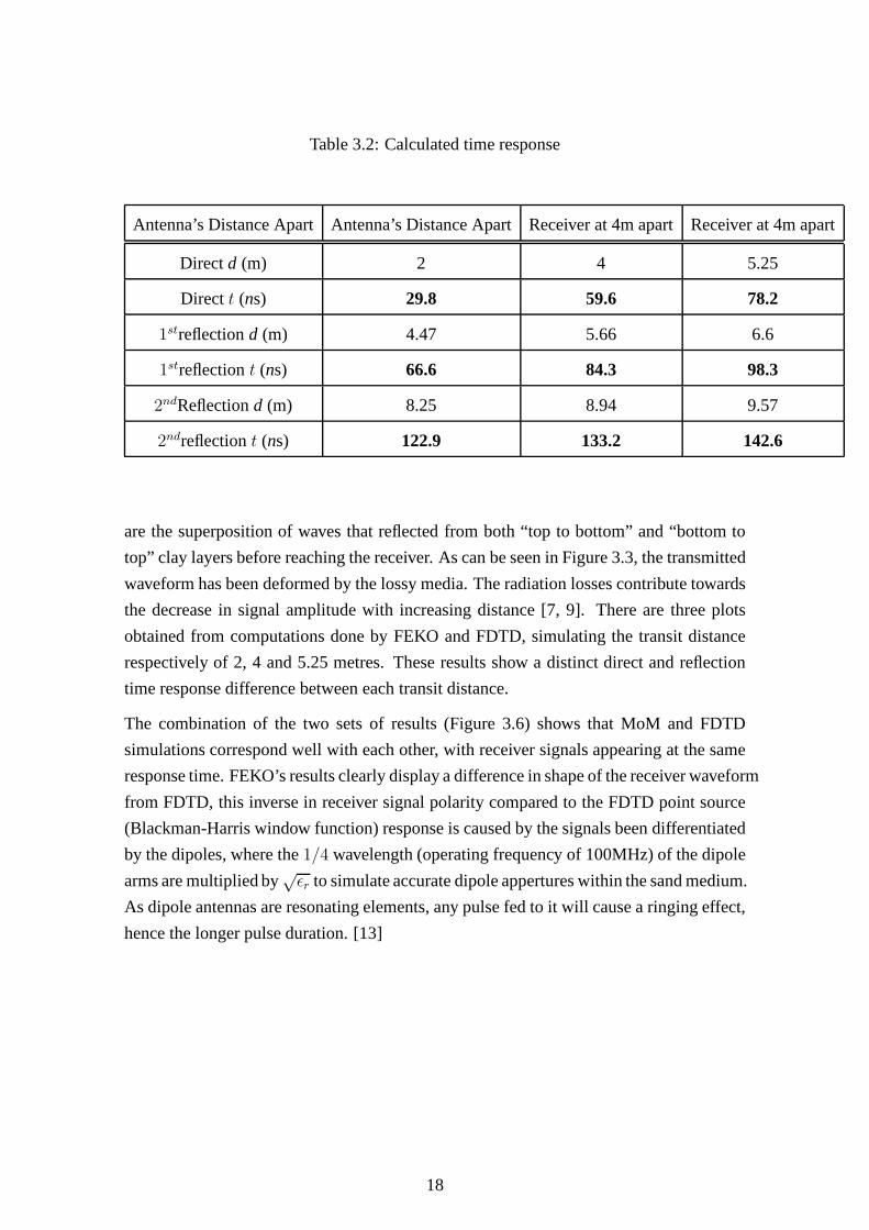
Table 3.2: Calculated time response

Antenna’s Distance Apart Antenna’s Distance Apart Receiver at 4m apartReceiver at 4m apart

Directd (m) 2 4 5.25

Direct t (ns) 29.8 59.6 78.2

1streflectiond (m) 4.47 5.66 6.6

1streflectiont (ns) 66.6 84.3 98.3

2ndReflectiond (m) 8.25 8.94 9.57

2ndreflectiont (ns) 122.9 133.2 142.6

are the superposition of waves that reflected from both “top to bottom” and “bottom to

top” clay layers before reaching the receiver. As can be seenin Figure 3.3, the transmitted

waveform has been deformed by the lossy media. The radiationlosses contribute towards

the decrease in signal amplitude with increasing distance [7, 9]. There are three plots

obtained from computations done by FEKO and FDTD, simulating the transit distance

respectively of 2, 4 and 5.25 metres. These results show a distinct direct and reflection

time response difference between each transit distance.

The combination of the two sets of results (Figure 3.6) showsthat MoM and FDTD

simulations correspond well with each other, with receiversignals appearing at the same

response time. FEKO’s results clearly display a differencein shape of the receiver waveform

from FDTD, this inverse in receiver signal polarity compared to the FDTD point source

(Blackman-Harris window function) response is caused by the signals been differentiated

by the dipoles, where the1/4 wavelength (operating frequency of 100MHz) of the dipole

arms are multiplied by√

ǫr to simulate accurate dipole appertures within the sand medium.

As dipole antennas are resonating elements, any pulse fed toit will cause a ringing effect,

hence the longer pulse duration. [13]

18

Figure 3.4: Received waveforms obtained using FEKO.

19

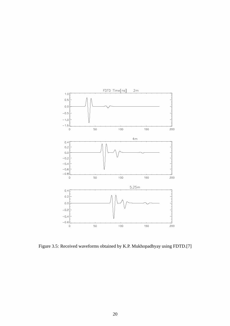
Figure 3.5: Received waveforms obtained by K.P. Mukhopadhyay using FDTD.[7]

20

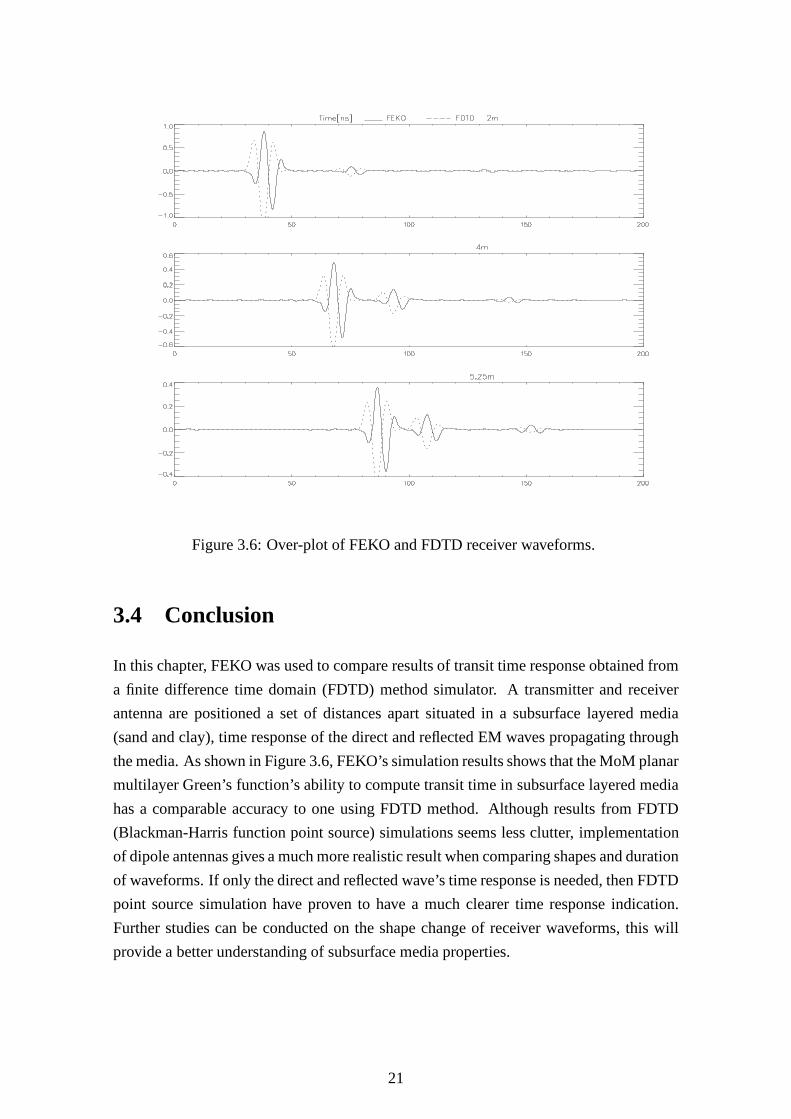
Figure 3.6: Over-plot of FEKO and FDTD receiver waveforms.

3.4 Conclusion

In this chapter, FEKO was used to compare results of transit time response obtained from

a finite difference time domain (FDTD) method simulator. A transmitter and receiver

antenna are positioned a set of distances apart situated in asubsurface layered media

(sand and clay), time response of the direct and reflected EM waves propagating through

the media. As shown in Figure 3.6, FEKO’s simulation resultsshows that the MoM planar

multilayer Green’s function’s ability to compute transit time in subsurface layered media

has a comparable accuracy to one using FDTD method. Althoughresults from FDTD

(Blackman-Harris function point source) simulations seems less clutter, implementation

of dipole antennas gives a much more realistic result when comparing shapes and duration

of waveforms. If only the direct and reflected wave’s time response is needed, then FDTD

point source simulation have proven to have a much clearer time response indication.

Further studies can be conducted on the shape change of receiver waveforms, this will

provide a better understanding of subsurface media properties.

21

Chapter 4

Fat Dipole Modelling

Antennas are one of the most critical elements in a ground penetrating radar system. For

this project they should satisfy a number of requirements including ultra wide frequency

bandwidth, low cross-coupling, short ringing effect and anunidirectional radiation pattern.

As GPR antennas operate very close to the ground and sometimes in contact with it, it

should be designed and constructed mechanically strong andyet mobile. Due to these

reasons, when obtaining a GPR antenna’s characteristics, it is required that to not only

measure them in free space but in a realistic ground penetrating environment. [20][21]

The fat dipole antenna is chosen to be investigated and modelled due to its simplicity in

design and UWB nature. Later on in this section, modificationwill be implemented to the

fat dipole design to improve its performance.

4.1 Modelling of UWB Fat Dipole Antenna

The UWB fat dipole in Figure 4.1 designed by the Korea Electro-technology Research

Institute (KERI) and Microline Co. Ltd. has been chosen to beinvestigated and modelled

for our GPR system due to its simplicity in design and its bandwidth performance. The

design has proven to have VSWR capability of below 2 at the bandwidth from 80MHz

to 310MHz shown in Figure 4.2. This section shows the resultssimulated by FEKO

compared to ones obtained by KERI and Microline.

22

Figure 4.1: Picture of KERI and Microline fat dipole[14]

Figure 4.2: 100 - 400MHz fat dipole VSWR[14]

The fat dipole from Figure 4.1 was modelled in FEKO shown below. This was done by

implementing the planar multilayer substrate function that incorporates Green’s function

to solve microstrip EM problems. The antenna dimensions includes dipole arms each

240mm x 500mm with 50mm gap between them, FR 4 (ǫr = 4.8) substrate, width of

1mm, and a grounding parabolic reflector used in KERI and Microline’s experiment.

Figure 4.6 is a FEKO graphical representation of the antenna:

23

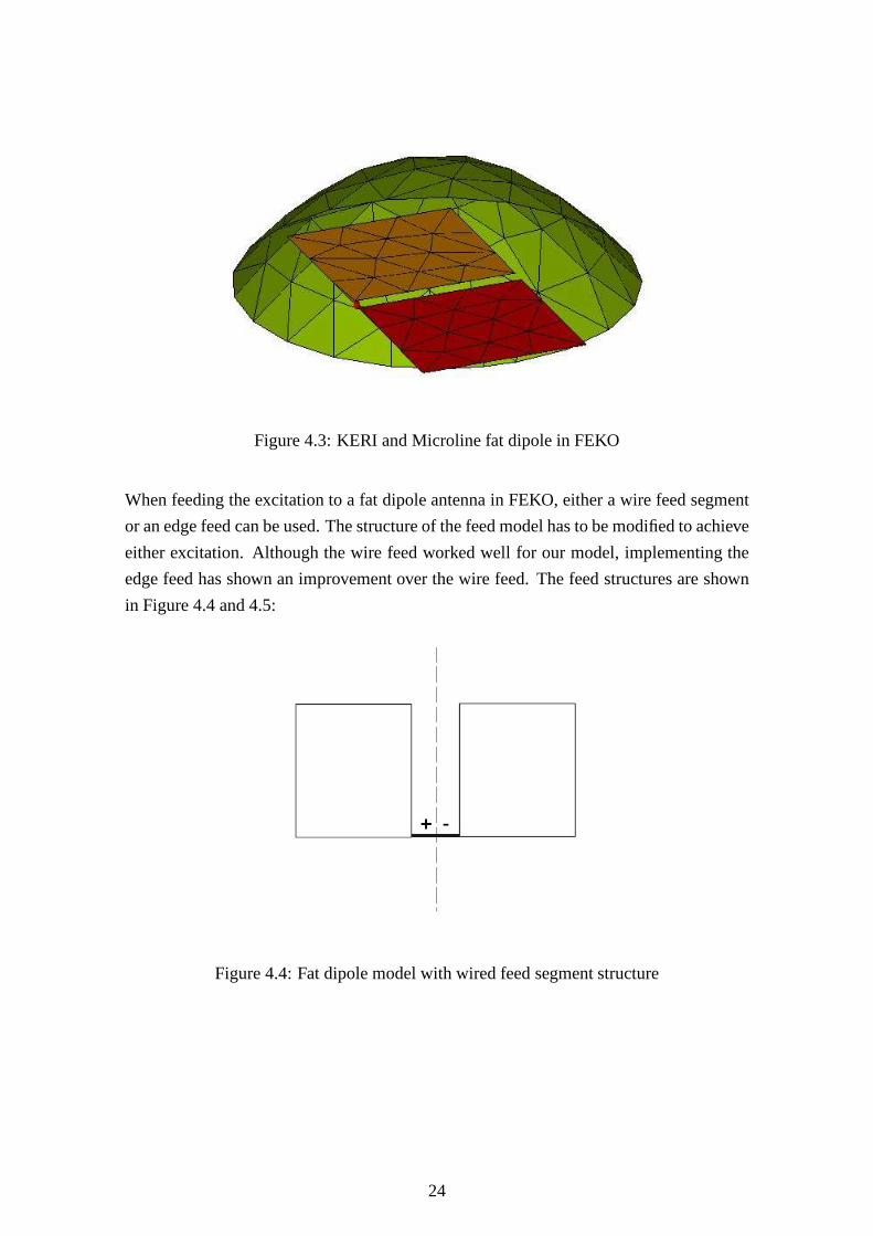
Figure 4.3: KERI and Microline fat dipole in FEKO

When feeding the excitation to a fat dipole antenna in FEKO, either a wire feed segment

or an edge feed can be used. The structure of the feed model hasto be modified to achieve

either excitation. Although the wire feed worked well for our model, implementing the

edge feed has shown an improvement over the wire feed. The feed structures are shown

in Figure 4.4 and 4.5:

Figure 4.4: Fat dipole model with wired feed segment structure

24

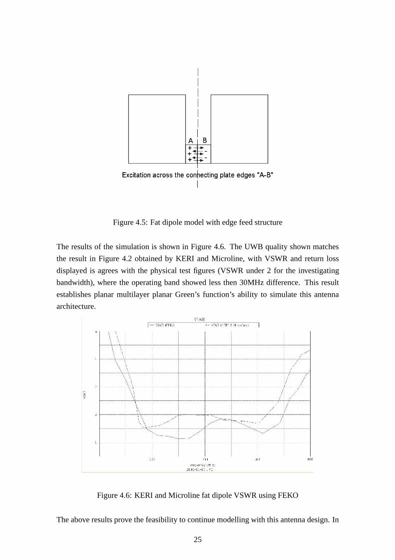
Figure 4.5: Fat dipole model with edge feed structure

The results of the simulation is shown in Figure 4.6. The UWB quality shown matches

the result in Figure 4.2 obtained by KERI and Microline, withVSWR and return loss

displayed is agrees with the physical test figures (VSWR under 2 for the investigating

bandwidth), where the operating band showed less then 30MHzdifference. This result

establishes planar multilayer planar Green’s function’s ability to simulate this antenna

architecture.

Figure 4.6: KERI and Microline fat dipole VSWR using FEKO

The above results prove the feasibility to continue modelling with this antenna design. In

25

the next section, adaptation of this design using a planar reflector for the 400-800MHz

region is attempted.

4.2 Modelling of 400 - 800MHz Fat Dipole

There are several modifications that have been implemented to fulfil this project’s specific

antenna requirements. In this case, the most important alteration is the change in physical

size of the radiating dipole arm to compensate for our specific operating bandwidth. A

polystyrene foam substrate was used instead of the FR-4 PCB substrate. This method

has proven to be highly effective for GPR applications as it allows the ground plate to

direct more energy back into the ground, increasing the efficiency of the antenna[14].

The antenna is also modelled 10mm above the ground due to variable ground surface in

a real GPR application. The ground’s electrical propertiesare set to the value of compact

sand, reason being this material is available for result validation at a later stage. Table 4.1

shows the substrates and ground properties.

Table 4.1: Dielectric Properties

Substrate FR-4 Polystyrene Ground (Sand)

Relative permittivityǫr 4.8 1.08 10

Electrical conductivity,σ [S/m] 1e−8 5e−14 1e−5

26

Figure 4.7: FEKO model of 400 - 800MHz fat dipole

To design the best fit antenna possible, several substrate heights have been modelled to

investigate how it affect the operating bandwidth and centre frequency of the antenna,

a graphical representation of this antenna is shown in Figure 4.7. The heights that are

chosen areλ/4,λ/8,λ/16 andλ/32 with the centre frequency being 600MHz. The reflection

coefficient of the antennas are shown in Figure 4.8.

27

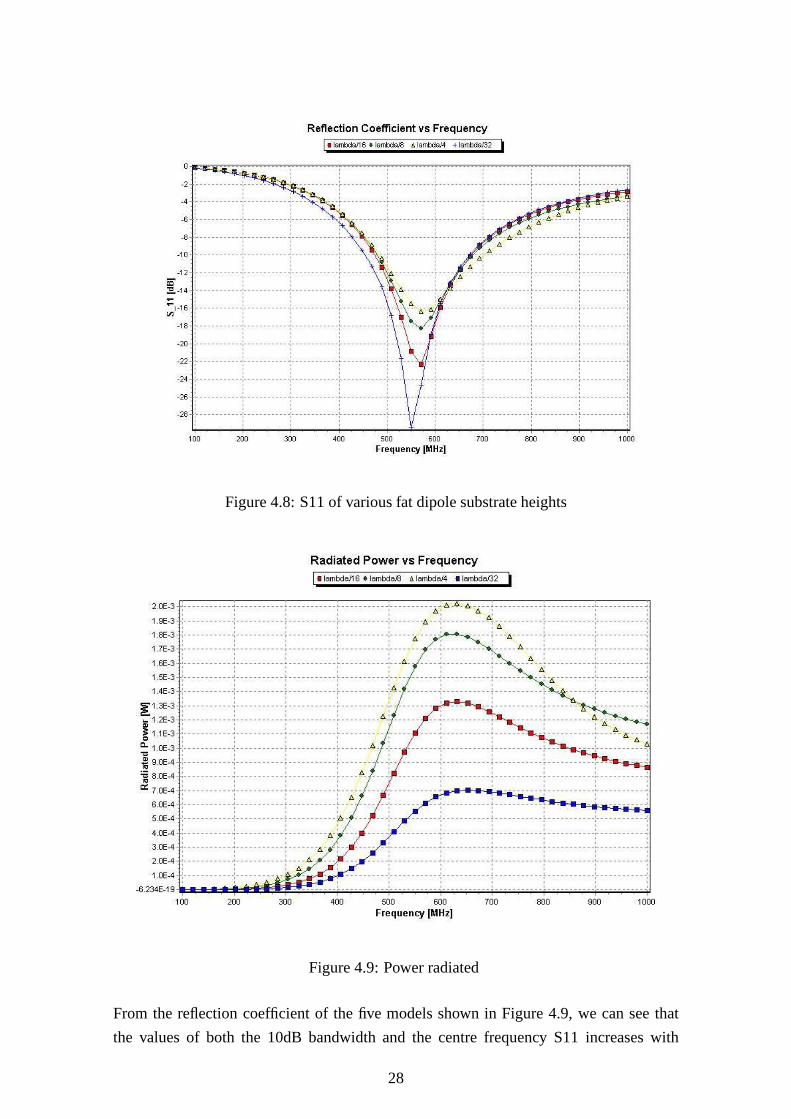
Figure 4.8: S11 of various fat dipole substrate heights

Figure 4.9: Power radiated

From the reflection coefficient of the five models shown in Figure 4.9, we can see that

the values of both the 10dB bandwidth and the centre frequency S11 increases with

28

decreasing substrate height, but can also be observed that radiated power decreases with

increasing height, where radiated power is obtained by using the excitation source data

function in FEKO, which calculate the radiated power from the input power less the

returned power at the feed point. Both of these properties are important when designing an

antenna. Although having a high radiated power is desired, it is crucial that it is radiated

in the correct direction, and in this case it must radiate mostly towards the ground. Figure

4.10 are the near field results along the z-axis which is the vertical axis perpendicular to

both the antenna and the ground surface. This indicates the amount of power radiating

into the ground, where z = 10mm is the point of contact with theground. From this we can

see that theλ/8 model proves to have the most power radiating into the desired direction

and was chosen for further development. The vertical radiation pattern displayed in the

Figure 4.11 shows that this dipole design has the directivity needed for GPR applications.

Figure 4.10: Electric near field indicating amount of power radiating vertically into theground

29

Figure 4.11: Fat dipole radiation pattern at 600MHz

4.3 Modelling of Cased Fat Dipole with Edge Terminating

Resistors

The current antenna design can be improved by constructing metallic barriers around

the polystyrene dielectric. This will direct more energy back into the forward direction

and also reduces the cross-coupling between the antennas. This structure also allows the

possibility of connecting the edge terminating resistors to the grounding metallic box.

Due to ground surface changes, it is also unlikely to have a fixed air gap with the ground

at all times, hence a 10mm thick Teflon plate is implemented toreplace the air gap. This

provides a layer of protection against abrasions that may occur to the aperture by the

ground terrain during GPR operation. This dielectric shielding of an antenna in a medium

has shown in previous studies observed by Stellenbosch University’s antenna research

group that the aperture dimensions can be reduced for the same operating frequency,

however with the trade-off of bandwidth and efficiency, depending on the thickness of the

dielectric[11]. The dimensions of the cased fat dipole consist of the two dipole arms being

133x140mm separated 14mm apart (approximately 10% of arm length) situated on top of

a polystyrene foam block of 280x140x62.5(λ/8 of 600MHz)mm, surrounding cavity of

280x140mm having a height of 52.5mm creating 10mm spacing between dipole arms and

30

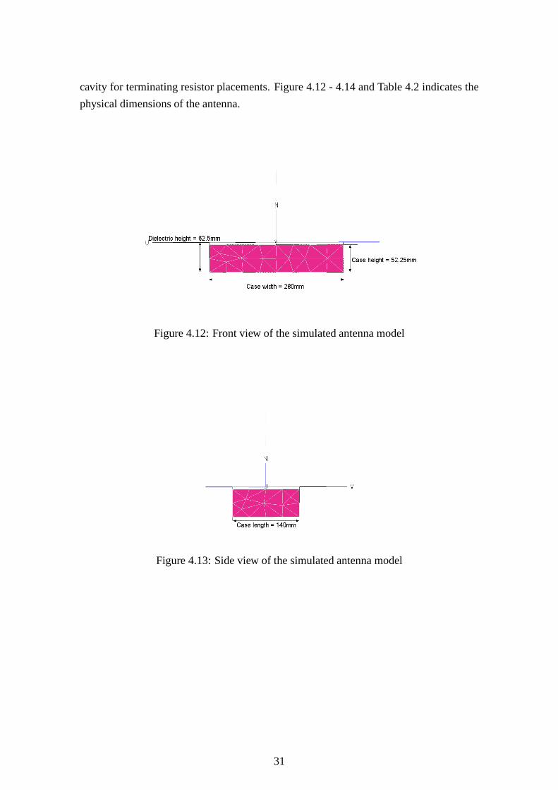
cavity for terminating resistor placements. Figure 4.12 - 4.14 and Table 4.2 indicates the

physical dimensions of the antenna.

Figure 4.12: Front view of the simulated antenna model

Figure 4.13: Side view of the simulated antenna model

31

Figure 4.14: Top view of the simulated antenna model

Table 4.2: Cased fat dipole Antenna simulation dimension inmm

Antenna Elements (mm) Width Length Height

Cavity 280 140 52.5

Aperture (per dipole arm) 133 140 0.5

Teflon Layer 280 140 10

Polystyrene Foam Dielectric 280 140 62.5 (λ/8)

Before modelling the antennas with terminating resistors,the impedance of the antenna

will have to be determined. As mentioned in Chapter 2, the terminating resistors are best

chosen to be of a higher value than the feed point impedance ofthe antenna. As shown

in Figure 4.15, the magnitude of the feed impedance can be observed to be an average of

210Ω across the operating band, hence250Ω terminating resistors were used to simulate

the antenna return loss. The terminating resistors are placed in the four edges of the box

connecting to the outer two edges of each arms of the dipole. Due to the plane of electrical

symmetry, these resistors will not influence the electricalfields within the antenna. Figure

4.16 illustrates the resistor connections.

32

Figure 4.15: Impedance and S11 simulated result before implementing terminatingresistors

33

Figure 4.16: Edge termination resistor connections

The improvement in antenna performance can be observed in Figure 4.17, illustrating the

effects of terminating resistors absorbing the low frequency reflections, hence increasing

the operating band of the fat dipole. The simulated electricnear field displayed in Figure

4.17 shown an improvement in efficiency compared to the result shown in Figure 4.10,

where by the casing of the dielectric has achieved maximising the transmission of energy

into the ground.

At the centre frequency of 660MHz, the 3D radiation pattern showed the desired unidirectional,

half hemisphere radiation pattern in the direction of the ground having approximately

10dB gain.

34

Figure 4.17: Improved S11 and near field result (at 600MHz) after implementingtermination resistors

35

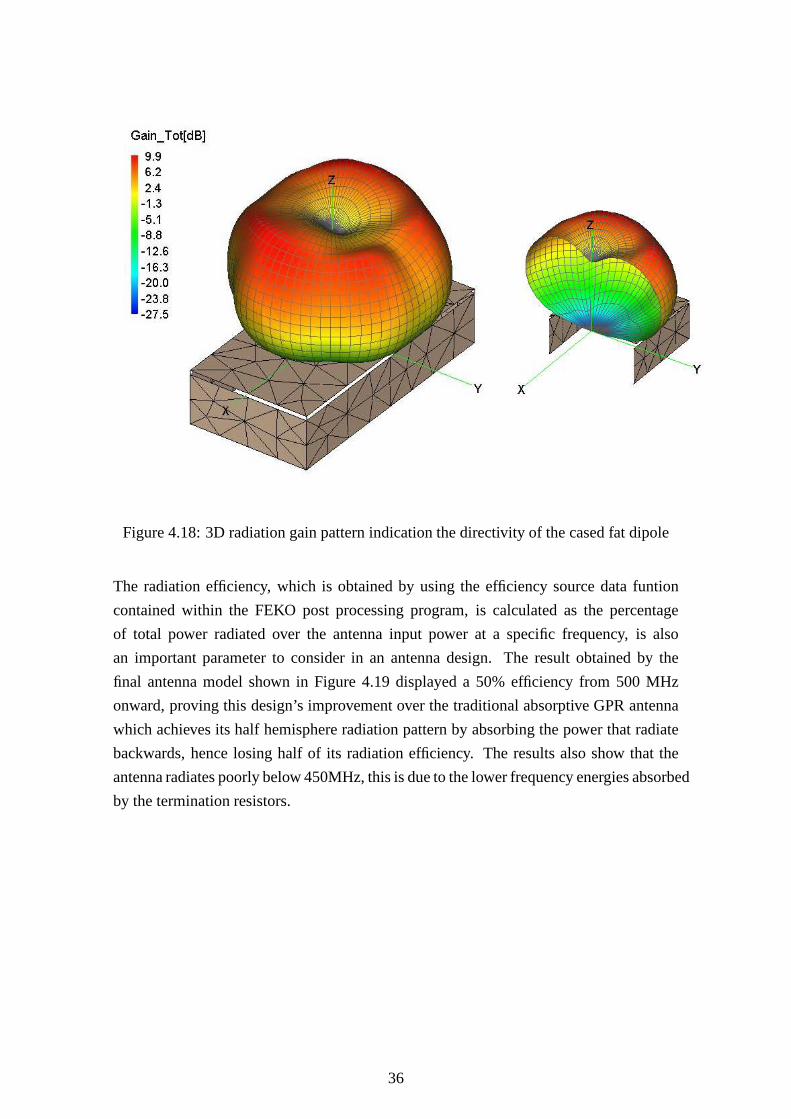
Figure 4.18: 3D radiation gain pattern indication the directivity of the cased fat dipole

The radiation efficiency, which is obtained by using the efficiency source data funtion

contained within the FEKO post processing program, is calculated as the percentage

of total power radiated over the antenna input power at a specific frequency, is also

an important parameter to consider in an antenna design. Theresult obtained by the

final antenna model shown in Figure 4.19 displayed a 50% efficiency from 500 MHz

onward, proving this design’s improvement over the traditional absorptive GPR antenna

which achieves its half hemisphere radiation pattern by absorbing the power that radiate

backwards, hence losing half of its radiation efficiency. The results also show that the

antenna radiates poorly below 450MHz, this is due to the lower frequency energies absorbed

by the termination resistors.

36

Figure 4.19: Radiation efficiency of the final antenna model

4.4 Conclusion

In Chapter 4, a 100-400MHz UWB fat dipole antenna designed byKorea Electro-technology

Research Institute (KERI) and Microline Co. Ltd. was reviewed. This design implements

the wide-band characteristics of an extended width patch dipole for GPR applications.

FEKO was used to model this antenna design and compare the simulated results with the

original developer’s VSWR. The results shown in Figure 4.6 validate the feasibility of

modelling such design in FEKO for this project.

After validation of the fat dipole design, several 400-800MHz dipoles were simulated

with different dielectric (polystyrene foam) and substrate height to investigate how its

effect the bandwidth, radiated power, electric near field and radiation pattern. This was

done to find the best suited antenna for fabrication and testing. Out of theλ/4,λ/8,λ/16

andλ/32 substrate heights, it was determined thatλ/8 is the best fit with regards to our

antenna requirement, which is having the maximum radiated power that is directed into

the ground.

With the GPR specifications in mind, an improved model was created using a Teflon

dielectric layer on the bottom of the aperture to protect theantenna from the ground (real

ground may have rough surfaces, hence a strong non-conductive material is needed for

37

protection against abrasion against the aperture). A cavity type design is also implemented

to maximise the energy directed into the ground, this designis validated with the simulation

results show in Figure 4.18 and 4.19. This design also provides conductive ground

for connecting edge terminating resistance to the aperture, where it has proven that it

has increased the operating bandwidth by reducing lower frequency reflections shown

in Figure 4.17. The next stage of this project is fabricatingthe modelled antenna and

verifying its performance.

38

Chapter 5

Antenna Construction and Verification

Through investigations done in the previous chapter, the cased fat dipole model showed

desired GPR antenna performance needed for this project. Inthis chapter, the method of

construction and return loss verification with the Agilent E5062A network analyser are

shown.

5.1 Antenna Aperture and Casing Construction

The antenna elements are constructed using 0.5mm tin plate due to it being the easiest

material to solder feed onto. The casing of the antenna is constructed using 1mm thick

aluminium plate, pop riveted to form a robust open ended box.The polystyrene dielectric

foam is then placed within the casing, with the dipole arms flush on top of the dielectric.

This configuration allows a 10mm gap between the aperture andthe aluminium casing for

connection of terminating resistors.

5.2 Balun Feed

A dipole antenna needs to have a balanced feed: this means equal current must feed into

each arms. A co-axial feed gives a positive source with reference to ground, hence it is

impossible to feed the two dipole arms directly. To solve this problem one would require

implementing a balun between the co-axial feed and the antenna. For this project, an

RF transformer is a suitable balun, as its provides impedance transformation between the

50Ω co-axial cable and the input impedance of the antenna, at thesame instance creating

a balanced to the dipole arms. For this antenna design, the transformer is required to feed

a50Ω co-axial to a210Ω impedance antenna. This is illustrated in Figure 5.1.

39

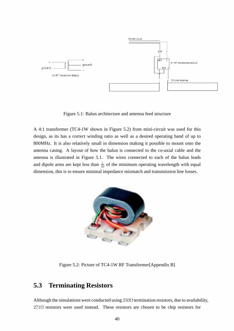
Figure 5.1: Balun architecture and antenna feed structure

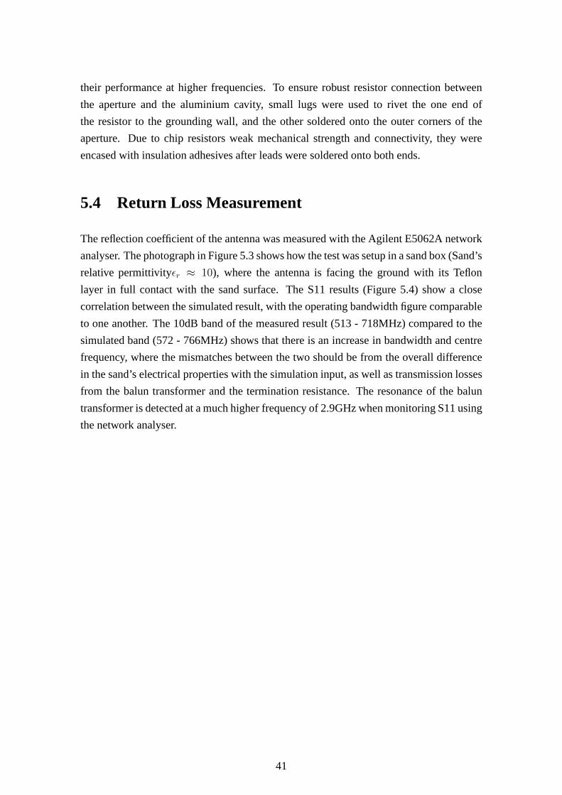
A 4:1 transformer (TC4-1W shown in Figure 5.2) from mini-circuit was used for this

design, as its has a correct winding ratio as well as a desiredoperating band of up to

800MHz. It is also relatively small in dimension making it possible to mount onto the

antenna casing. A layout of how the balun is connected to the co-axial cable and the

antenna is illustrated in Figure 5.1. The wires connected toeach of the balun leads

and dipole arms are kept less than110

of the minimum operating wavelength with equal

dimension, this is to ensure minimal impedance mismatch andtransmission line losses.

Figure 5.2: Picture of TC4-1W RF Transformer[Appendix B]

5.3 Terminating Resistors

Although the simulations were conducted using250Ω termination resistors, due to availability,

271Ω resistors were used instead. These resistors are chosen to be chip resistors for

40

their performance at higher frequencies. To ensure robust resistor connection between

the aperture and the aluminium cavity, small lugs were used to rivet the one end of

the resistor to the grounding wall, and the other soldered onto the outer corners of the

aperture. Due to chip resistors weak mechanical strength and connectivity, they were

encased with insulation adhesives after leads were soldered onto both ends.

5.4 Return Loss Measurement

The reflection coefficient of the antenna was measured with the Agilent E5062A network

analyser. The photograph in Figure 5.3 shows how the test wassetup in a sand box (Sand’s

relative permittivityǫr ≈ 10), where the antenna is facing the ground with its Teflon

layer in full contact with the sand surface. The S11 results (Figure 5.4) show a close

correlation between the simulated result, with the operating bandwidth figure comparable

to one another. The 10dB band of the measured result (513 - 718MHz) compared to the

simulated band (572 - 766MHz) shows that there is an increasein bandwidth and centre

frequency, where the mismatches between the two should be from the overall difference

in the sand’s electrical properties with the simulation input, as well as transmission losses

from the balun transformer and the termination resistance.The resonance of the balun

transformer is detected at a much higher frequency of 2.9GHzwhen monitoring S11 using

the network analyser.

41

Figure 5.3: Photograph of the antennas and S11 sand box testing arrangement withAgilent E5062A network analyser

42

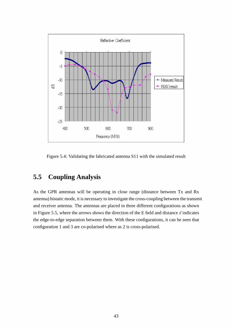
Figure 5.4: Validating the fabricated antenna S11 with the simulated result

5.5 Coupling Analysis

As the GPR antennas will be operating in close range (distance between Tx and Rx

antenna) bistatic mode, it is necessary to investigate the cross-coupling between the transmit

and receiver antenna. The antennas are placed in three different configurations as shown

in Figure 5.5, where the arrows shows the direction of the E field and distanced indicates

the edge-to-edge separation between them. With these configurations, it can be seen that

configuration 1 and 3 are co-polarised where as 2 is cross-polarised.

43

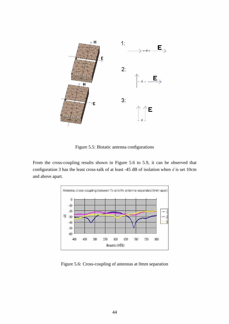
Figure 5.5: Bistatic antenna configurations

From the cross-coupling results shown in Figure 5.6 to 5.9, it can be observed that

configuration 3 has the least cross-talk of at least -45 dB of isolation whend is set 10cm

and above apart.

Figure 5.6: Cross-coupling of antennas at 0mm separation

44



Figure 5.9: Cross-coupling of antenna at 15mm separation

45

5.6 Object Detection

The final test conducted in this chapter is investigating whether the antennas are capable

of object detection. As shown in Figure 5.10, the antennas are placed above a 60x60mm

wide metal plate buried 15cm beneath the sand’s surface. Dueto surface area limitations,

only eight samples were taken at 2cm intervals within close proximity above the metal

plate. The Tx and Rx antennas are separated 10cm apart implementing configuration 3

(Figure 5.5) defined in the previous section. This setup has proven to have minimal cross-

coupling while keeping both antennas at a close proximity toeach other. These sampling

displacement intervals are illustrated below:

Figure 5.10: Sand box object detection test configuration

S12 insertion loss between the Tx and Rx antennas were taken at each points illustrated

in Figure 5.10. The eight sample values are then inverse Fourier transformed to obtain

the corresponding time-domain response which are displayed in Figure 5.11, where the

y-axis shows the displacement at which the antennas are placed to obtain insertion losses

and the x-axis displaying the depth at which response occurs. Due to unknown fix delay in

antennas and cables, the depth information is set to be zero from where maximum surface

reflections are observed. The results shown correspond to the depth displacement of the

buried metal plate where the region labelled “time response” contains the difference in

time response signals between the samples. The first three samples have a longer delayed

response as the receiver antenna are located further away from the object. The following

four equivalent response matches the equal distances travelled between the antennas as

it is located right on top of the flat metal plate. The last signal represent the slightly

shorter response due to the receiver antenna situated directly on top of the object, hence

46

less time needed for the signal to travel. There are strong concurrent response detected

at shallow depth, observed within the dotted barrier labelled “ground reflections”, this is

due to initial sand surface reflections.

Figure 5.11: Time-domain object detection results of a metal plate buried at a depth of15cm

5.7 Conclusion

In this chapter, the construction and testing methods of theantenna is shown and discussed.

The S11 results obtained from the network analyser shows that although the 10dB band

of the measured (513 - 718MHz) and the simulated band (572 -766MHz) shows close

correlation, it still has a increase in bandwidth. This is due to the difference in sand’s

electrical properties from the simulation input, as well astransmission losses from the

balun transformer and the termination resistors. Besides simulation validation, coupling

analysis and object detection were also conducted. The results shown in Section 5.5

concludes that Tx and Rx antenna placement implementing configuration 3 (Figure 5.5)

will have minimal cross-coupling. The buried metal plate detection experiment using the

network analyser has also proven that the antennas are realistically capable of transmitting

47

and detecting response from objects buried in sand.

48

Chapter 6

Conclusions and Recommendations

This chapter includes conclusions drawn from the results obtained in Chapters 3, 4 and 5.

6.1 Ground penetration transmitter-receiver time response

simulations done in FEKO and FDTD

FEKO’s simulation results shows that the MoM planar multilayer Green’s function’s

ability to compute transit time in subsurface layered mediahas a comparable accuracy

to one using FDTD method. Although results from FDTD (Blackman-Harris function

point source) simulations seems less cluttered due to less attenuation, implementation of

dipole antennas gives a much more realistic result when comparing shapes and duration

of waveforms. If only the direct and reflected wave’s time response is needed, then

FDTD point source simulation have proven to have a less attenuated. Further studies

can be conducted on the shape change of receiver waveforms, this will provide a better

understanding of subsurface media properties.

6.2 GPR fat dipole modelling

The design and modelling of a 400 - 800MHz ultra wide-band GPRantenna was successfully

investigated, fabricated and validated. The fat dipole design have been implemented and

modified to the desired operating bandwidth. The following objectives have been met

with the improved metallic cased fat dipole design:

• The edge terminations resistors have proven to reduce reflections from lower frequencies

hence improving the operating bandwidth.

49

• Both impedance matching and balun implementation has been resolved by means

of a RF transformer, thus reducing the cost and complexity ofthe antenna.

• The metallic casing of the polystyrene dielectric region has allowed the antenna to

achieve the directive half hemisphere radiation pattern required for a GPR application.

• The extremely low permittivity and conductivity of expanded polystyrene dielectric

region implemented in this design has proven to have a much improved radiation

efficiency over the traditional absorptive GPR antennas. Itprovides an efficiency

of 50% and above from 450MHz onward, where as the absorptive antennas has a

trade-off in losing half it efficiency in order to obtain the half hemisphere radiation

effect.

• The cross-coupling measurement has shown that when operating these antennas

in a GPR application, the transmit and receiver antenna should be placed at a co-

polarised position shown in antenna configuration 3 (Figure5.5). This will provide

at least -45dB isolation within the operating bandwidth.

• The object detection experiment conducted has proven that the fat dipole antennas

are realistically capable of transmitting and detecting response from objects buried

in sand.

This investigation has proven that FEKO is a practical tool for simulating UWB antennas.

Its implementation of the multilayer Green’s function for computing dielectric substrate

has given good indications of how design elements affect thereflection coefficient and

efficiency of the antenna.

6.3 Future work

The following GPR experiments can be investigated to improve the antenna’s performance:

1. A sandbox with greater surface area can be constructed so that further test in object

detection can be done with more sampling intervals to improve result definition.

2. Metal object of different shapes can be buried to compare the change in scattered

response.

3. Further GPR Field work, such as the detection of buried pipes and subsurface void,

can be done to test the feasibility of the antennas in realistic applications.

4. Different construction methods of this antenna design can be implemented and

research into various dielectric materials to improve the robustness of the cased

fat dipole.

50

Appendix A

Software Source Code

A.1 FEKO Code

A.1.1 Subsurface Transit Response - EDITFEKO

This part of the code contains the experimented methods of using dielectric bodies, as

well as Green’s multi-layer functions, in order to define thesand and clay regions needed

for Transit Response simulations.

****** Frequency and wavelength

!!if (not(defined(#freq))) then

#freq = 100.0e6

!!endif

#scaling = 1

#maxfreq = 2e9

#lam = #c0/#maxfreq

********** Define the edge length *********************

#edge_len = (2 - #freq/#maxfreq)*#lam/4

** #edge_len = #lam/4

********** Parameters for segmentation**************** **

#seg_rad = #lam/1000 ** radius of the wire segments\

#seg_len = #lam/20 ** maximum length of wire segments

*******maximum edge length - Defined for experimentations with dielectric bodies

** #tri_len = #lam/100

51

#l = 0.4*#seg_len

IP #seg_rad #seg_len

************************* -Borehole defined for experimentations with dielectric bodies

** ** Borehole

** DP a 0.032 -0.032 2

** DP b -0.032 -0.032 2

** DP c 0.032 0.032 2

** DP d 0.032 -.032 0

** QU a b c d 1 0 0.00000001

************************ - Sand layer defined for experimentations with dielectric

bodies

** ** Sand Layer

** DP A 1 0 2

** DP B 0 0 2

** DP C 1 2.75 2

** DP D 1 0 0

** LA 1

** QU A B C D 1 0 0.001

********************** **- Sand layer defined for experimentations with dielectric

bodies

** Clay Layer

** DP E 1 0 2

** DP F 0.5 0 2

** DP G 1 2.75 2

** DP H 1 0 0

** LA 2

** QU E F G H 40 0.5 1073

************************ -Second sand layer defined for experimentations with dielectric

bodies

** ** Sand Layer

** DP a 0.5 0 1

52

** DP b 0 0 1

** DP c 0.5 1.375 1

** DP d 0.5 0 0

** LA 1

** QU a b c d 20 0.0001 1800

** ** clay

** DP e 1 0 1

** DP f 0.5 0 1

** DP g 1 1.375 1

** DP h 1 0 0

** LA 2

** QU e f g h 40 0.005 1073

**

** ** SY 1 0 1 1

************** Length defined for Dipole Antennas******** *******

#U = #lam/4

#D = -#lam/4

#Ul = #l

#Dl =-#l

********************Transmitter******************** *********

DP A 0 0 -#U

DP B 0 0 -#l

DP C 0 0 #l

BL A B

SY 1 0 0 3

LA 1

BL B C

TG 1 0 1 1 0 5.25

*********Receiver Placements************************ ************

** LA 1

53

** BL T3 T4

**

** LA 2

** DP R3 0 4 #Ul

** DP R4 0 4 #Dl

** BL R3 R4

**

** LA 3

** DP T3 0 -1 #Ul

** DP T4 0 -1 #Dl

** DP T5 0 -1 #D

** BL T4 T5

** BL T3 T4

**

** LA 4

** DP R3 0 1 #Ul

** DP R4 0 1 #Dl

** DP R5 0 1 #D

** BL R4 R5

** BL R3 R4

** ************Apply the scaling factor*************

SF 1 #scaling

************** End of geometric input*************

** EG 1 0 0 0 20 0.0001 1073 1

EG 1 0 0 0 1

*************************************************** *********

** Set the frequency

FR 1 #freq

** Excitation

A1 0 1 1 0 50

54

FF 0

** FF 1 1 1 0 90 90 0 0

**********Green’s Function Multi-layer - ground layers (Sand and Clay)***********

GF 12 3 0 2.2

0.2 40 1 0.5

4 20 1 0.0001

0.2 40 1 0.5

** Receiver current

OS 4 2 1

** End

EN

A.1.2 Subsurface Transit Response - TIMEFEKO

** Define the Pulse form

GAUSS

** Parameters of the Gaussian pulse

** Time shift Exponent

10e-9 300e6

FREQUENCY

** Upper frequency Number of Samples

225e6 46

** Normalise the time to that of the speed of light

** NORM

** Output the excitation

EXCITATION

A.1.3 KERI and Microline Co. Ltd Fat Dipole - EDITFEKO

#freq = 300e+6

#lam = 1000*(#c0/#freq)

55

SF 1 0.001

** #seg_rad = 0.01

** #seg_len = 10

** #tri_len = 10

** IP #seg_rad #tri_len #seg_len

************ Import model BIG dipole**************

IN 8 31 "FD.cfm"

** ** ******* Import model dipole ******************

** IN 8 31 "FDs.cfm"

** End of geometry

EG 1 0 0 0 1

** Set frequency

FR 21 0 0.1e+08 4.1e+08

GF 10 2 0 10 1 1e-5 0

1 4.8 1 0

200 1 1 0

** DI Poly 2.3 1 5e-4

** GF 10 1 0 10 1 1e-5 10

** 72.5 2.3 1 5e-4

** SP 50

******************Experimentations of Various Dipole Fe ed******************

** A4 0 -1 0 1 0 3 1 0

AE: 0 : dipole.feed : dipole.feed1 : 0 : : 1

** AE 0 a b 3 1

** A4 0 -1 1 1 0 0 0 0 0.65

** A4: 0 : Polygon2.Face36 : 0 : : : 1 : : 0 : 0 : 0

** A1: 0 : dipole.feed : : : : 1

OS 2 0

** OF 1 0 0 20 0

** End of file

EN

56

A.1.4 Improved 400 - 800 MHz Fat Dipole - EDITFEKO

#freq = 300e+6

#lam = 1000*(#c0/#freq)

SF 1 0.001

** #seg_rad = 0.01

** #seg_len = 10

** #tri_len = 10

** IP #seg_rad #tri_len #seg_len

** *****Import model Cased Fat Dipole

IN 8 31 "FD.cfm"

EG 1 0 0 0 1

** Set frequency

FR 21 0 0.1e+08 4.1e+08

GF 10 2 0 10 1 1e-5 0

1 4.8 1 0

200 1 1 0

** DI Poly 2.3 1 5e-4

** GF 10 1 0 10 1 1e-5 10

** 72.5 2.3 1 5e-4

** SP 50

**************** Set Source and Experimentation Excitati ons*****************

** A4 0 -1 0 1 0 3 1 0

AE: 0 : dipole.feed : dipole.feed1 : 0 : : 1

** AE 0 a b 3 1

** A4 0 -1 1 1 0 0 0 0 0.65

** A4: 0 : Polygon2.Face36 : 0 : : : 1 : : 0 : 0 : 0

** A1: 0 : dipole.feed : : : : 1

OS 2 0

** OF 1 0 0 20 0

** End of file

EN

57

A.2 IDL Code

IDL code was used to display the time-domain result calculated by TIMEFEKO

A.2.1 Subsurface Time Response - Graphical Display

;————–Antenna Distance 2m———-

filename = "ground2m.aus"

header1 = strarr(12+128+8+128+7) ;283

array1 = fltarr(4,128) ;4

header2 = strarr(6) ;6


openr, lun, filename, /get_lun

readf, lun, header1, array1, header2, array2

close,lun

Xaxis1 = array1[0,*]

Yaxis1 = array1[3,*] ;3


Yaxis2 = array2[1,*]

fx = findgen(n_elements(Xaxis1))

gx = findgen(n_elements(Xaxis1)*10)/10

fy = findgen(n_elements(Yaxis1))

gy = findgen(n_elements(Yaxis1)*10)/10

curve1x = (interpol(Xaxis1, fx, gx))/1e-9 ;Interpolation


curve1y = (interpol(Yaxis1, fy, gy, /spline))/1.5e-8 ;Interpolation


;————Antenna Distance 4m————–


header3 = strarr(12+128+8+128+7) ;283


58





close,lun













;————–Antenna Distance 5.25m————


header5 = strarr(12+128+8+128+7) ;283






close,lun





59









;————FDTD Import—————

aa = fltarr(3,1300)

openr,1,’nbor_Ez_h4_x246.dat’

readu,1,aa

close,1

time = fltarr(1300)

openr,1,’time.dat’

readu,1,time

close,1

;———–plot—————–

!p.multi = [0,1,3]

plot, curve1x, curve1y

oplot,time,(aa(0,*)/1e-4), linestyle = 3





currdevice=!D.NAME

set_plot,’ps’

device, filename = ’combination.eps’, /encapsulated, preview=2, xsize=6, ysize=4.5,/inches

!p.multi = [0,1,3]

plot, curve1x, curve1y, title = ’Time[ns] ____ FEKO —- FDTD 2m’ ;Plot label

60


plot, curve3x, curve3y, title = ’ 4m’


plot, curve5x, curve5y, title = ’ 5.25m’


device, /close

set_plot, currdevice

currdevice=!D.NAME

set_plot,’ps’

device, filename = ’receiverFDTD.eps’, /encapsulated, preview=2, xsize=3.4, ysize=4,/inches

;Encapsulating the result.

plot,time,(aa(0,*)/1e-4), title = ’FDTD Time[ns] 2m’

plot,time,(aa(1,*)/1e-4), title = ’ 4m’

plot,time,(aa(2,*)/1e-4), title = ’ 5.25m’

device, /close

set_plot, currdevice

end

A.2.2 Object Detection

; These are the code used to display the object detection results obained by the Agilent

E5062A network analyser.

;————-Data Extraction———–

num_freq = 200

S12_data = dblarr(10, num_freq)

;filename = ’S12_object_detection.txt’

filename = ’try.txt’

openr, u_file,filename,/Get_Lun

readf,u_file,S12_data

free_lun,u_file

freq = reform(s12_data(0,*))

61

xpos_0 = reform(s12_data(1,*))

useless = reform(s12_data(2,*))








;———–Data Plot———————

fs = 800e6

dt = 1/fs

t = findgen(200)*dt

df = (fs/(num_freq))+400e6

ddt = 1/df

tt = findgen(200)*ddt

dsp = tt*(3e8)/(3.16)

td = (1/(freq))

tdd = findgen(200)*td

;dist = td*3e8/3.16

dist =findgen(200)/35

x1 = fft(xpos_0,-1)

x2 = fft(xpos_2,-1)

x3 = fft(xpos_4,-1)

x4 = fft(xpos_6,-1)

x5 = fft(xpos_8,-1)

x6 = fft(xpos_10,-1)



F1 = findgen(n_elements(x1))

62

F1i = findgen(n_elements(x1)*10)/10















Fd = findgen(n_elements(dist))

Fdi = findgen(n_elements(dist)*10)/10

curve1x = (interpol(x1, f1, f1i, /spline)) ;Interpolation








curvedist = (interpol(dist, fd, fdi));Interpolation

plot, curvedist, (curve1x), xrange = [0, 0.5], yrange = [-a,38*a], title = ’Depth(m)’

oplot, curvedist, (curve2x + a*5)



63





end

64

Appendix B

TC4-1W Balun Transformer Data Sheet

65

Bibliography

[1] GeoModel, “Ground Penetrating Radar Basic Operating Principals”,

www.geomodel.com/gprtext.htm, GeoModel, Inc.March 2005.

[2] Saul Rodriguez Duenas, “Ultra Wide Band Systems”,

www.imit.kth.se/courses/2B1457/Lecture05/lecture7_UWB_lecture_Saul.pdf,

KTH,2005.

[3] Mathworld, “Green’s Function”, mathworld.wolfram.com/GreensFunction.html,

WOLFRAM RESEARCH,September 2004.

[4] NI Developer Zone, “Windowing: Optimizing FFTs Using Window Functions”,

National Instruments, June 2005.

[5] R. Clarke, R. Karunaratni, C. Schrader, “Ultra-Wide Band Antenna”,College of

Engineering, San Jose State University.Fall 2004.

[6] EM Software & Systems-S.A. (Pty) Ltd, “FEKO User’s Manual”, FEKO 48.294,

PREFEKO 27.55-60 and later, June 2004.

[7] K.P. Mudhopadhyay, M.R. Inggs and A.J. Wilkinson, “FTDTModelling of a

Borehole Radar Wave Propagation: a 3-D Simulation Study in aConductive Media”,

International Geoscience and Remote Sensing Symposium, pp 109–126, 2005.

[8] K.P. Mudhopadhyay, “Three-Dimensional Finite Difference Time Domain

Modelling of Borehole Radar in mining applications”,Radar and Remote Sensing

Group, Department of Electrical Engineering, University of Cape Town, South

Africa, 2004.

[9] P.W Futter, “Advance Modelling of a Borehole Radar Environment with the FDTD

Method”,Matieland, South Africa, Stellenbosch University, 2001.

[10] Guy Atkin, “T2FD–The Forgotten Antenna”, www.hard-core-

dx.com/nordicdx/antenna/wire/t2fd.html, HCDX Antennas, April 2002.

67

[11] Max Birch, “Development of a Cavity Backed Bowtie Antenna with Dielectric

Matching for Ground Penetrating Radar”,Matieland, South Africa, University of

Stellenbosch,September 2001

[12] Alex Peeters, “Transmission Line Theory”,www.citap.com/documents/tcp-

ip/tcpip021.htm, TCI-IP Networks, March 2003.

[13] Enrico M. Staderini, “A Pratical Imtroduction to UltraWideband Technology”,Tor

Vergata University of Rome, 2004

[14] Korea Electrotechnology Research Institute (KERI) & Microline Co., Ltd., “Buried

Small Object Detected by UWB GPR”,Proc. of Asia Pacific Microwave Conference

2003 (APMC’03), 2003

[15] D. Jeffrereys, “www.ee.surrey.ac.uk/Personal/D.Jeffreys/mmethod.html”,Technical

report, University of Surrey, 2004

[16] Seok H Choi, Jong K. Park, Sun K. Kim and Jae Y. Park, “A NewUltra-Wideband

Antenna For UWB Applications”,Department of Radio Wave Engineering, Hanbat

National University, August 2003

[17] J. Silvertrim, “IEEE Ultra wideband Presentation”,Innovative Wireless

Technologies, 1047 Vista Park Drive Suite A, Forest,October 2003

[18] David Kinnon, “Identification of Land Mine using Microwave Resonance

Signature”,University of Queensland, October 1999

[19] A.A Lestari, A.G Yarovoy, L.P. Ligthart, “Capacitively-Tapered Bowtie Antenna”,

International Research Center for Telecommunications-Transmision and Radar,

Delft University of Technology, Faculty of Information Technology and Systems,

2003

[20] A.G Yarovoy, L.P. Lighart, “Ultra-Wideband Antennas for Ground Penetrating

Radar”, International Research Center for Telecommunications-Transmision and

Radar, Delft University of Technology, Faculty of Information Technology and

Systems, 2003

[21] A.G Yarovoy, P.J. Aubrey, L.P. Lighart, “GPR Antenna Measurements in Time

Domain”, International Research Center for Telecommunications-Transmision and

Radar, Delft University of Technology, Faculty of Information Technology and

Systems, 2003

[22] Hans Gregory Schantz, “Radiation Efficiency of UWB Antennas”,Proceedings of

the 2002 IEEE UWBST Conference, 2002.

68

[23] D.M. Pozar, ”Microwave and RD Design of Wireless Systems”, John Wiley and

Sons, 2001

69

gpr propagation simulation and fat dipole antenna...

Documents